searching for brown dwarf companions
TRANSCRIPT

Searching for Brown DwarfCompanions
November 2008
Avril C. Day-Jones
A report submitted in partial fulfillment of the requirements of the University ofHertfordshire for the degree of Doctor of Philosophy.

2

Abstract
In this thesis I present the search for ultracool dwarf companions to main sequence stars,subgiants and white dwarfs. The ultracool dwarfs identified here are benchmark objects,with known ages and distances.
The online data archives, the two micron all sky survey (2MASS) and SuperCOS-MOS were searched for ultracool companions to white dwarfs, where one M9±1 companionto a DA white dwarf is spectroscopically confirmed as the widest separated system of itskind known to date. The age of the M9±1 is constrained to a minium age of 1.94Gyrs,based on the estimated age of the white dwarf from a spectroscopically derived Teff andlog g and an initial-final mass relation. This search was extended using the next gener-ation surveys, the sloan digital sky survey (SDSS) and the UK infrared deep sky survey(UKIDSS), where potential white dwarf + ultracool dwarf binary systems from this searchare presented. A handful of these candidate systems were followed-up with second epochnear infrared (NIR) imaging. A new white dwarf with a spectroscopic M4 companion anda possible wide tertiary ultracool component is here confirmed.
Also undertaken was a pilot imaging survey in the NIR, to search for ultracoolcompanions to subgiants in the southern hemisphere using the Anglo-Australian telescope.The candidates from that search, as well as the subsequent follow-up of systems throughsecond epoch NIR/optical imaging and methane imaging are presented. No systems areconfirmed from the current data but a number of good candidates remain to be followed-upand look encouraging.
A search for widely separated ultracool objects selected from 2MASS as compan-ions to Hipparcos main-sequence stars was also undertaken. 16 candidate systems wererevealed, five of which had been previously identified and two new L0±2 companions arehere confirmed, as companions to the F5V spectroscopic system HD120005 and the Mdwarf GD 605. The properties of HD120005C were calculated using the DUSTY andCOND models from the Lyon group, and the age of the systems were inferred from theprimary members. For GD 605B no age constraint could be placed due to the lack ofinformation available about the primary, but HD120005C has an estimated age of 2-4Gyr.
In the final part of this thesis I investigate correlations with NIR broadband colours(J − H, H − K and J − K) with respect to properties, Teff , log g and [Fe/H] for thebenchmark ultracool dwarfs, both confirmed from the searches undertaken in this workand those available from the literature. This resulted in an observed correlation with NIRcolour and Teff , which is presented here. I find no correlation however with NIR coloursand log g or [Fe/H], due in part to a lack of suitable benchmarks. I show that despitethe current lack of good benchmark objects, this work has the potential to allow UCDproperties to be measured from observable characteristics, and suggest that expanding thisstudy should reveal many more benchmarks where true correlation between properties andobservables can be better investigated.
3

4

Acknowledgments
I would like to extend a thank you to all the people who have provided help andsupport throughout my Ph.D. no matter how large or small, your help was always appre-ciated.
I firstly need to thank my supervisors David Pinfield, Hugh Jones and Ralf Napi-wotzki for their constant support and help with every aspect of the Ph.D, for their patienceand understanding and for teaching me the skills needed to succeed.
I could also not have done this Ph.D. without the support, both emotionally andfinancially from all of my immediate and extended family.
I also owe a very big thank you to James Jenkins, who helped me with manyscientific and computing aspects throughout my Ph.D, as well as his tireless support,encouragement, motivation and constant belief in me throughout.
I would also like to thank my fellow students and inhabitants of Starlink for theirhelp, support and hundreds of cups of tea over the last 3 years, with a special thanksto Bob Chapman, Stuart Folkes, Douglas Weights and Krispian Lowe for all their manyhours of help with IDL, IRAF and LATEX.
I also extend a thank you to the staff and grad students at Penn State University,who made it possible for me to work there during the summer of 2008 and for the fantasticexperience I had while I was there.
I also owe thanks to Harriet Parsons, Simon Weston, Andy Gallagher and JoannaGoodger for providing a temporary roof and their sofas/floors for the last months of mywrite up.
Thank You to you all!
I would like to dedicate this thesis to my grandmother Joyceline Pay, who passed awayduring the last weeks of writing this thesis, I know she would have been proud to see itcome to fruition.
5

6

Contents
1 Background 17
1.1 Introduction . . . . . . . . . . . . . . . . . . . . . . . . . . . . . . . . . . . 17
1.1.1 Properties of brown and ultracool dwarfs . . . . . . . . . . . . . . . 18
1.2 Benchmark ultracool dwarfs . . . . . . . . . . . . . . . . . . . . . . . . . . 23
1.2.1 Ultracool formation scenarios . . . . . . . . . . . . . . . . . . . . . 24
1.3 The ultracool IMF and birthrate . . . . . . . . . . . . . . . . . . . . . . . 26
1.3.1 The substellar initial mass function . . . . . . . . . . . . . . . . . . 26
1.3.2 The substellar birth rate . . . . . . . . . . . . . . . . . . . . . . . . 28
1.3.3 Ultracool evolution . . . . . . . . . . . . . . . . . . . . . . . . . . . 30
1.4 Understanding and interpretation of ultracool atmospheres . . . . . . . . . 31
1.4.1 Atmospheric models . . . . . . . . . . . . . . . . . . . . . . . . . . 32
1.4.2 Benchmark UCDs as members of binary systems . . . . . . . . . . . 35
1.4.3 Stellar evolution beyond the main-sequence . . . . . . . . . . . . . . 37
1.5 Motivation and thesis structure . . . . . . . . . . . . . . . . . . . . . . . . 43
2 Selection Techniques 45
2.1 Selecting white dwarfs . . . . . . . . . . . . . . . . . . . . . . . . . . . . . 46
2.1.1 White dwarfs in SuperCOSMOS . . . . . . . . . . . . . . . . . . . . 46
2.1.2 White dwarfs in SDSS . . . . . . . . . . . . . . . . . . . . . . . . . 47
2.2 Selecting ultracool dwarfs . . . . . . . . . . . . . . . . . . . . . . . . . . . 50
2.2.1 L dwarfs in 2MASS . . . . . . . . . . . . . . . . . . . . . . . . . . . 50
2.2.2 L and T dwarfs in UKIDSS . . . . . . . . . . . . . . . . . . . . . . 52
7

3 Ultracool companions to white dwarfs 57
3.1 Selecting candidate binary pairs . . . . . . . . . . . . . . . . . . . . . . . . 57
3.2 Searching SuperCOSMOS and 2MASS . . . . . . . . . . . . . . . . . . . . 58
3.2.1 Proper motions of candidate systems . . . . . . . . . . . . . . . . . 62
3.3 A wide WD + UCD binary . . . . . . . . . . . . . . . . . . . . . . . . . . 63
3.3.1 Spectral classification of UCDc-1: 2MASSJ0030-3739 . . . . . . . . 63
3.3.2 Spectral classification of WDc-1: 2MASSJ0030-3740 . . . . . . . . . 68
3.3.3 A randomly aligned pair? . . . . . . . . . . . . . . . . . . . . . . . 72
3.3.4 Binary age . . . . . . . . . . . . . . . . . . . . . . . . . . . . . . . . 73
3.3.5 UCD properties . . . . . . . . . . . . . . . . . . . . . . . . . . . . . 74
3.4 Searching SDSS and UKIDSS . . . . . . . . . . . . . . . . . . . . . . . . . 74
3.4.1 Simulated numbers of WD + UCD binaries . . . . . . . . . . . . . 74
3.4.2 Binary selection . . . . . . . . . . . . . . . . . . . . . . . . . . . . . 76
3.4.3 Candidate WD + UCD systems . . . . . . . . . . . . . . . . . . . . 79
3.4.4 Second epoch imaging and proper motion analysis of candidate UCDs 81
3.4.5 A candidate wide L dwarf companion to a spectroscopic WD + Mdwarf binary . . . . . . . . . . . . . . . . . . . . . . . . . . . . . . . 94
3.5 Summary of chapter . . . . . . . . . . . . . . . . . . . . . . . . . . . . . . 100
4 Ultracool companions to Subgiants 101
4.1 A pilot survey of southern Hipparcos subgiants . . . . . . . . . . . . . . . . 101
4.1.1 Selection of subgiants . . . . . . . . . . . . . . . . . . . . . . . . . . 101
4.1.2 Simulated populations . . . . . . . . . . . . . . . . . . . . . . . . . 102
4.2 The pilot survey . . . . . . . . . . . . . . . . . . . . . . . . . . . . . . . . . 104
4.2.1 Observing strategy . . . . . . . . . . . . . . . . . . . . . . . . . . . 107
4.2.2 Extraction and calibration of photometry . . . . . . . . . . . . . . . 107
4.2.3 Selection of good candidate systems . . . . . . . . . . . . . . . . . . 111
4.3 Follow-up Observations . . . . . . . . . . . . . . . . . . . . . . . . . . . . . 114
4.3.1 Second epoch imaging . . . . . . . . . . . . . . . . . . . . . . . . . 117
4.3.2 Methane imaging . . . . . . . . . . . . . . . . . . . . . . . . . . . . 119
4.4 Discussion . . . . . . . . . . . . . . . . . . . . . . . . . . . . . . . . . . . . 124
8

5 Ultracool companions to main-sequence stars 127
5.1 Selection of Hipparcos main-sequence + UCD wide binary systems . . . . . 127
5.2 Spectroscopic follow-up observations . . . . . . . . . . . . . . . . . . . . . 131
5.2.1 Reduction and extraction of data . . . . . . . . . . . . . . . . . . . 131
5.3 Spectral classifications . . . . . . . . . . . . . . . . . . . . . . . . . . . . . 134
5.3.1 Cand 13 . . . . . . . . . . . . . . . . . . . . . . . . . . . . . . . . . 134
5.3.2 Cand 10 . . . . . . . . . . . . . . . . . . . . . . . . . . . . . . . . . 136
5.4 Parameters of the systems . . . . . . . . . . . . . . . . . . . . . . . . . . . 139
5.4.1 Gl605 . . . . . . . . . . . . . . . . . . . . . . . . . . . . . . . . . . 139
5.4.2 HD120005 . . . . . . . . . . . . . . . . . . . . . . . . . . . . . . . . 141
5.5 Discussion . . . . . . . . . . . . . . . . . . . . . . . . . . . . . . . . . . . . 142
6 Further discussion and conclusions 145
6.1 The ultracool mass-age distribution . . . . . . . . . . . . . . . . . . . . . . 145
6.2 The current benchmark population . . . . . . . . . . . . . . . . . . . . . . 146
6.2.1 Open clusters and moving groups . . . . . . . . . . . . . . . . . . . 150
6.2.2 UCDs in binaries . . . . . . . . . . . . . . . . . . . . . . . . . . . . 157
6.2.3 Field UCDs . . . . . . . . . . . . . . . . . . . . . . . . . . . . . . . 164
6.3 Discussion . . . . . . . . . . . . . . . . . . . . . . . . . . . . . . . . . . . . 166
6.3.1 The effects of gravity and metallicity on observed UCD properties . 170
6.3.2 Correlations with colour and physical properties . . . . . . . . . . . 172
6.4 Future Work . . . . . . . . . . . . . . . . . . . . . . . . . . . . . . . . . . . 182
9

10

List of Figures
1.1 Optical spectra of an M9, L3 and L8 types from Kirkpatrick et al. (1999). . 20
1.2 NIR spectra of M7-L2 dwarfs from Reid et al. (2001). . . . . . . . . . . . . 21
1.3 NIR spectra of L3.5-L8 dwarfs from Reid et al. (2001). . . . . . . . . . . . 21
1.4 NIR spectra of T dwarfs from Burgasser et al. (2003). . . . . . . . . . . . . 22
1.5 Main-sequence mass function from Miller & Scalo (1979). . . . . . . . . . . 27
1.6 Pleiades mass function from Lodieu et al. (2007) . . . . . . . . . . . . . . . 29
1.7 Bolometric luminosity functions from Allen et al. (2005). . . . . . . . . . . 30
1.8 Comparison of Φ(Teff) for different birth rate scenarios from Burgasser etal. (2004). . . . . . . . . . . . . . . . . . . . . . . . . . . . . . . . . . . . . 31
1.9 Cooling tracks for brown dwarfs, stars and planets taken from Burrows etal. (1997). . . . . . . . . . . . . . . . . . . . . . . . . . . . . . . . . . . . . 32
1.10 Hertzsprung-Russell diagram . . . . . . . . . . . . . . . . . . . . . . . . . . 36
1.11 Cooling tracks for DA WDs from Chabrier et al. (2000). . . . . . . . . . . 41
1.12 The initial-final-mass-relation for WDs from Dobbie et al. (2006). . . . . . 41
2.1 A reduced proper motion diagram of WD candidates from SuperCOSMOS 48
2.2 A reduced proper motion diagram of WDs from SDSS DR2 from Kilic etal. (2006). . . . . . . . . . . . . . . . . . . . . . . . . . . . . . . . . . . . . 50
2.3 A u− g against g − r two colour diagram of WDs selected from SDSS (DR6) 51
2.4 A J − H against H − K two colour diagram of L dwarfs from dwar-
farchives.org. . . . . . . . . . . . . . . . . . . . . . . . . . . . . . . . . 53
2.5 A Y −J against J−H two colour diagram showing L and T dwarf selectionregions. . . . . . . . . . . . . . . . . . . . . . . . . . . . . . . . . . . . . . 55
3.1 A WD MB against B −R absolute colour-magnitude diagram for McCook& Sion (1999) WDs with known parallax. . . . . . . . . . . . . . . . . . . . 59
3.2 Separation area probed by 2MASS and SuperCOSMOS for WD + UCDbinaries. . . . . . . . . . . . . . . . . . . . . . . . . . . . . . . . . . . . . . 60
11

3.3 An MJ against J − K absolute colour-magnitude diagram showing com-panion UCD candidates. . . . . . . . . . . . . . . . . . . . . . . . . . . . . 62
3.4 SuperCOSMOS and 2MASS images show UCDc-1 (2MASSJ0030 − 3739)and WDc-1 (2MASSJ0030 − 3740). . . . . . . . . . . . . . . . . . . . . . . 64
3.5 J- band spectra of UCDc-1 (2MASSJ0030 − 3739) . . . . . . . . . . . . . . 66
3.6 H- band spectra of UCDc-1 (2MASSJ0030 − 3739) . . . . . . . . . . . . . 66
3.7 Optical spectrum of the confirmed white dwarf WDc-1 (2MASSJ0030−3740). 69
3.8 Model atmosphere fit to the Balmer lines of 2MASSJ0030 − 3740. . . . . . 71
3.9 Simulated WD + UCD J- against g- magnitude diagram from Pinfield etal. (2006) . . . . . . . . . . . . . . . . . . . . . . . . . . . . . . . . . . . . 76
3.10 A WD Mg against g − r colour-magnitude diagram for McCook & Sion(1999) WDs with known parallax . . . . . . . . . . . . . . . . . . . . . . . 77
3.11 A UCD colour-magnitude diagram for L and T dwarfs with known parallaxfrom dwarfarchives.org. . . . . . . . . . . . . . . . . . . . . . . . . . . 78
3.12 Left: i − z against spectral type relation. Right: z − J against spectraltype relation from Hawley et al. (2002). . . . . . . . . . . . . . . . . . . . 80
3.13 Colour-colour relations for M, L and T dwarfs from Hawley et al. (2002).. . 80
3.14 Left: A Y − J against J − H two-colour diagram. Right: An MJ againstJ −H CMD of UCD candidate components of potential wide WD + UCDbinaries. . . . . . . . . . . . . . . . . . . . . . . . . . . . . . . . . . . . . . 82
3.15 A u−g against g−r two colour diagram showing WD candidate componentsof potential wide WD + UCD binaries. . . . . . . . . . . . . . . . . . . . . 83
3.16 SDSS spectra of the WD candidate nBIN7. . . . . . . . . . . . . . . . . . . 95
3.17 Model DA4 WD SDSS spectra combined with M0-L0 spectra. . . . . . . . 97
3.18 Model DA5 WD SDSS spectra combined with M0-L0 spectra. . . . . . . . 98
3.19 Model DA4 WD SDSS combined with an M4 spectra. . . . . . . . . . . . . 99
3.20 M4 component of the convolved spectra of nBIN7. . . . . . . . . . . . . . . 99
4.1 Subgiant selection.(a) An MV against B − V diagram of Hipparcos starswith V < 13.0 and π/σ ≥ 4. (b) Theoretical isochrones from Girardi etal. (2000) for solar metallicity. . . . . . . . . . . . . . . . . . . . . . . . . . 103
4.2 Simulated distance - magnitude distribution of UCD companions to Hip-parcos subgiants from Pinfield at al. (2006). . . . . . . . . . . . . . . . . . 105
4.3 Predicted separation-distance distribution of subgiant + UCD binaries. . . 106
4.4 A diagram showing the imaging strategy used for the subgiant survey onAAT/IRIS2. . . . . . . . . . . . . . . . . . . . . . . . . . . . . . . . . . . . 108
4.5 An airmass curve for standard star observations. . . . . . . . . . . . . . . . 110
12

4.6 A J−H against ∆ magnitude plot showing the zero point calibration using2MASS objects for the J- band for one IRIS2 imaging field. . . . . . . . . 111
4.7 A plot of magnitude against the difference in flux between two aperturesizes in the J- band for objects in one image. . . . . . . . . . . . . . . . . . 112
4.8 A J − H against Y − J two-colour diagram, showing the position of mainsequence stars, M, L and T dwarfs. . . . . . . . . . . . . . . . . . . . . . . 114
4.9 Left: A J −H against Z −J two-colour diagram, showing candidate L andT dwarfs. Right: A MJ against J − H CMD of L and T dwarf candidates. 115
4.10 Plot from Tinney et al. (2005) showing the position of the methane filters;CH4s and CH4l. . . . . . . . . . . . . . . . . . . . . . . . . . . . . . . . . 120
4.11 A CH4s − CH4l colour against spectral type plot from Tinney et al. (2005).121
4.12 A CH4s − CH4l against CH4s CMD for Cand T18. . . . . . . . . . . . . . 123
5.1 Top: MJ against J − K CMD for candidate L dwarf companions to Hip-parcos stars. Bottom: A distance - separation plot for the candidate main-sequence + L dwarf binary systems. . . . . . . . . . . . . . . . . . . . . . . 129
5.2 A vector point diagram of four candidate main sequence + L dwarf commonproper motion systems. . . . . . . . . . . . . . . . . . . . . . . . . . . . . . 131
5.3 The ZJ spectrum of Cand 13. . . . . . . . . . . . . . . . . . . . . . . . . . 132
5.4 The HK spectrum of Cand 13. . . . . . . . . . . . . . . . . . . . . . . . . . 133
5.5 The HK spectrum of Cand 10. . . . . . . . . . . . . . . . . . . . . . . . . . 133
5.6 The ZJ spectrum of Cand 13 overplotted with template spectra (M7, M8,M9, L0.5, L1 and L2 type) from Cushing, Rayner & Vacca (2005). . . . . . 137
5.7 The HK spectrum of Cand 13, overplotted with template spectra (M7, M8,M9, L0.5, L1 and L2 type) from Cushing, Rayner & Vacca (2005). . . . . . 138
5.8 The HK band spectrum of Cand 10, overplotted with template spectra(M7, M8, M9, L0.5, L1 and L2 type) from Cushing, Rayner & Vacca (2005).140
6.1 Simulations of the UCD mass-age population from Pinfield et al. (2006) for2MASS and UKIDSS. . . . . . . . . . . . . . . . . . . . . . . . . . . . . . . 147
6.2 Simulations of the UCD mass-age population from Pinfield et al. (2006) forUCD companions to WDs and subgiants. . . . . . . . . . . . . . . . . . . . 148
6.3 The mass-age distribution of benchmark UCDs from the literature andboth confirmed and candidate objects presented in this work . . . . . . . . 167
6.4 Teff against log g for benchmark UCDs taken from the literature and bothconfirmed and candidate objects presented in this work. . . . . . . . . . . . 168
6.5 Teff against Fe/H for benchmark UCDs taken from the literature and bothconfirmed and candidate objects presented in this work. . . . . . . . . . . . 169
13

6.6 MJ against J −K colour space showing the dependence of metallicity andgravity on models from Burrows et al. (2006) for their COND and DUSTYmodels. . . . . . . . . . . . . . . . . . . . . . . . . . . . . . . . . . . . . . 173
6.7 Teff against J − K space predictions of the DUSTY and COND modelsfrom Burrows et al. (2006). . . . . . . . . . . . . . . . . . . . . . . . . . . . 173
6.8 Left: MJ as a function of spectral type and Right: MJ as a function ofJ − K colour for L and T dwarfs from Knapp et al. (2004). . . . . . . . . . 174
6.9 Teff against colour plot of benchmark L dwarfs with NIR J − H, H − Kand J − K colours. . . . . . . . . . . . . . . . . . . . . . . . . . . . . . . . 175
6.10 Teff against colour plot of benchmark T dwarfs with NIR J − H, H − Kand J − K colours. . . . . . . . . . . . . . . . . . . . . . . . . . . . . . . . 175
6.11 Colour against log g, where the colour-Teff trend has been subtracted fromthe colour, for benchmark L dwarfs with NIR J − H, H − K and J − Kcolours. . . . . . . . . . . . . . . . . . . . . . . . . . . . . . . . . . . . . . 177
6.12 Colour against log g, where the colour-Teff trend has been subtracted fromthe colour, for benchmark T dwarfs with NIR J − H, H − K and J − Kcolours. . . . . . . . . . . . . . . . . . . . . . . . . . . . . . . . . . . . . . 177
6.13 Colour against Fe/H, where the colour-Teff trend has been subtracted fromthe colour, for benchmark L dwarfs with NIR J − H, H − K and J − Kcolours. . . . . . . . . . . . . . . . . . . . . . . . . . . . . . . . . . . . . . 178
6.14 Colour against Fe/H, where the colour-Teff trend has been subtracted fromthe colour, for benchmark T dwarfs with NIR J − H, H − K and J − Kcolours. . . . . . . . . . . . . . . . . . . . . . . . . . . . . . . . . . . . . . 178
6.15 Improved Teff against colour plot, where the effects of log g and Fe/H havebeen removed for the benchmark L dwarfs with NIR J − H, H − K andJ − K colours. . . . . . . . . . . . . . . . . . . . . . . . . . . . . . . . . . 181
14

List of Tables
1.1 The classification scheme for WDs from Sion et al. (1983). . . . . . . . . . 40
2.1 Galactic co-ordinates of contaminated and overcrowded regions removed. . 52
3.1 Candidate UCD + WD binary systems from SuperCOSMOS and 2MASS. 61
3.2 Estimated spectral types for 2MASSJ0030 − 3739. . . . . . . . . . . . . . . 68
3.3 Fit results and derived quantities for WD mass, cooling age and absolutemagnitude for 2MASSJ0030 − 3740. . . . . . . . . . . . . . . . . . . . . . . 70
3.4 Parameters of the binary 2MASSJ0030− 3739 + 2MASSJ0030− 3740 andits components. . . . . . . . . . . . . . . . . . . . . . . . . . . . . . . . . . 75
3.5 Parameters of the WD component of the WD + UCD binary candidateswith optical counterparts selected from SDSS and UKIDSS. . . . . . . . . 84
3.6 Parameters of the UCD component of the WD + UCD binary candidateswith optical counterparts selected from SDSS and UKIDSS. . . . . . . . . 85
3.7 Parameters of the WD component of the WD + late M dwarf binary can-didates selected from SDSS and UKIDSS. . . . . . . . . . . . . . . . . . . 86
3.8 Parameters of the UCD component of the WD + late M dwarf binarycandidates selected from SDSS and UKIDSS. . . . . . . . . . . . . . . . . . 87
3.9 Parameters of the WD component of the WD + UCD i- band drop outbinary candidates selected from SDSS and UKIDSS. . . . . . . . . . . . . . 88
3.10 Parameters of the UCD component of the WD + UCD i- band drop outbinary candidates selected from SDSS and UKIDSS. . . . . . . . . . . . . . 89
3.11 Parameters of the WD component of the WD + UCD non-optical detectionbinary candidates selected from SDSS and UKIDSS. . . . . . . . . . . . . . 90
3.12 Parameters of the UCD component of the WD + UCD non-optical detec-tion binary candidates selected from SDSS and UKIDSS. . . . . . . . . . . 92
3.13 Proper motion analysis for followed up candidate WD + UCD binary pairsfrom SDSS and UKIDSS . . . . . . . . . . . . . . . . . . . . . . . . . . . . 94
4.1 Candidate subgiant + UCD binary systems. . . . . . . . . . . . . . . . . . 116
15

4.2 Proper motion measurements of candidate L and early T dwarfs. . . . . . . 119
4.3 The status of UCD candidates (confirmed or not). . . . . . . . . . . . . . . 126
5.1 Widely separated main sequence + L dwarf candidate systems. . . . . . . . 130
5.2 Spectral ratios for Cand 13 . . . . . . . . . . . . . . . . . . . . . . . . . . . 135
5.3 Equivalent widths for Cand 13 . . . . . . . . . . . . . . . . . . . . . . . . . 135
5.4 Spectral ratios for Cand 10 . . . . . . . . . . . . . . . . . . . . . . . . . . . 139
5.5 Parameters of the system HD12005 . . . . . . . . . . . . . . . . . . . . . . 143
6.1 Subgiant + UCD candidates with age and mass constraints estimated fromthe Lyon group DUSTY and COND models. . . . . . . . . . . . . . . . . . 151
6.2 Main-sequence + UCD Candidates with known ages and masses derivedfrom the Lyon group DUSTY and COND models. . . . . . . . . . . . . . . 152
6.3 Cluster and Moving Group UCDs. . . . . . . . . . . . . . . . . . . . . . . . 155
6.4 Pleiades cluster UCDs. . . . . . . . . . . . . . . . . . . . . . . . . . . . . . 156
6.5 UCD in binaries . . . . . . . . . . . . . . . . . . . . . . . . . . . . . . . . . 161
6.6 UCD + WD binaries . . . . . . . . . . . . . . . . . . . . . . . . . . . . . . 163
6.7 Field UCDs with age estimates . . . . . . . . . . . . . . . . . . . . . . . . 165
6.8 Parameters of fitting equations for colours of T dwarfs. . . . . . . . . . . . 180
6.9 Parameters of fitting equations for colours of L dwarfs. . . . . . . . . . . . 180
16

Chapter 1
Background
.
In this chapter the background knowledge relevant to the later chapters in this thesis
is discussed. In brief the main topics here include an overview of the understanding and
interpretation of ultracool dwarf (UCD) and brown dwarf (BD) atmospheres, formation
scenarios, the ultracool contribution to the initial mass function and the birth rate of L
and T dwarfs are also discussed in context. A particular emphasis is given to benchmark
UCDs, why they are needed, how they will be used and where they can be found.
1.1 Introduction
In just over a decade nearly 700 UCDs have been discovered since those that were first
confirmed (Tiede 1 (M8); Rebolo, Zapatero-Osorio & Martin 1995 and Gliese 229B (T6.5);
Nakajima et al. 1995). This is in large thanks to the rise of deep large area surveys such as
the Two Micron All Sky Survey (2MASS), the Sloan Digital Sky Survey (SDSS) and more
recently the UK Infrared Deep Sky Survey (UKIDSS). These populations have helped
shape the understanding of ultracool dwarfs and extended the classification system for
substellar objects including the creation of two new spectral types L and T. The latest M
dwarfs (∼M7-9) have effective temperature (Teff) reaching down to ∼2300K. At lower Teff
(∼2300-1400K) are the L dwarfs, which have very dusty upper atmospheres and generally
very red colours. T dwarfs are even cooler having Teff in the range ∼1400-600K, where
the low Teff limit is currently defined by the recently discovered T8+ dwarfs, ULAS J0034-
0052 (Warren et al. 2007), CFBDS J005910.90-011401.3 (Delorme et al. 2008) and ULAS
17

1335 (Burningham et al. 2008). T dwarf spectra are dominated by strong water vapour
and methane bands, and generally appear bluer in the near infrared (NIR) (Geballe et al.
2003; Burgasser, Burrows & Kirkpatrick 2006).
The physics of ultracool atmospheres is complex and very difficult to accurately
model. Atmospheric dust formation is particularly challenging for theory (Allard et al.
2001; Burrows, Sudarsky & Hubeny 2006) and there are a variety of other important issues
that are not well understood, including the completeness of CH4/H2O molecular opacities,
their dependence on Teff , gravity and metallicity (e.g. Jones et al. 2005; Burgasser et al.
2006; Liu, Leggett & Chiu 2007), as well as the possible presence of vertical mixing in such
atmospheres (Saumon et al. 2007). The emergent spectra from ultracool atmospheres are
likely strongly affected by factors such as gravity and metallicity (e.g. Knapp et al.
2004; Burgasser et al. 2006; Metchev & Hillenbrand 2006), which highlights the need
for an improved understanding of such effects if physical properties (e.g. mass, age and
composition) are to be constrained observationally (e.g. spectroscopically).
Discovering UCDs whose properties can be inferred indirectly (without the need for
atmospheric models) is an excellent way to provide a test-bed for theory and observa-
tionally pin down how physical properties affect spectra. Such UCDs are referred to as′benchmark′ objects (e.g. Pinfield et al. 2006). A population of benchmark UCDs with
a broad range of atmospheric properties will be invaluable in the task of determining
the full extent of spectral sensitivity to variations in UCD physical properties. However,
such benchmarks are not common and the constraints on their properties are not always
particularly strong.
1.1.1 Properties of brown and ultracool dwarfs
BDs were first theorised by Kumar (1963) as a cool extension of the main-sequence, beyond
the M7 type. They are not massive enough to ignite or burn hydrogen in their core, such
that an upper mass limit would correspond approximately to 0.075M� (Chabrier et al.
2000a), although it is possible for this limit to change with metallicity (if the BD is metal
poor then it can have a larger mass). The lower end of the mass limit remains ill defined
approaching the planetary mass regime. The difference between BDs and giant planets
is commonly assumed to be the way in which they form. It was originally suspected that
BDs form in the same way as stars, from the fragmentation of a gas cloud (as shown by
the simulations of Bate 1998) and that giant planets form via accretion onto rocky cores
18
in a proto-planetary disk (e.g. Pollack et al. 1996). However the formation mechanisms
for both types of object are not fully understood. The currently adopted lower mass
limit is taken from the deuterium burning minimum mass (0.013M�), which draws the
distinction that all BDs burn deuterium at some point during their lifetime. However
Bate (2005) showed that the minimum mass (i.e. the deuterium burning limit) of a BD
can change by 3-9 MJup from simulating clouds where the opacity limit is set by the clouds
metallicity, such that metallicity can drive this mass up towards 0.015M�. This has also
been challenged more recently by the discovery of planetary mass objects in Orion (Lucas
et al. 2006; Weights et al. 2008) and 2MASS1207B, an 8±2MJup L dwarf (Mohanty et al.
2007).
For ages of a few Gyr, these masses correspond to temperatures generally less than
∼2300K (Kirkpatrick et al. 1999b) encompassing two new spectral classifications, the L
and T dwarfs (Kirkpatrick et al. 1999b; Martın et al. 1999). Traditionally spectral typing
is done using optical spectra as is typically done for L dwarfs, following the conventions
of Kirkpatrick et al. (1999b). However, as L dwarfs are faint at these wavelengths it is
often easier to use NIR spectra. Indeed T dwarfs are very faint in the optical and are
thus formally classified in the NIR following the classification scheme of Burgasser et al.
(2006). In general L and T dwarfs are BDs but objects later than ∼M7 can be referred
to as UCDs. From an M dwarf a UCD is expected to cool and evolve through the L to
the T dwarf sequence and to cooler temperatures (Kirkpatrick et al. 1999b).
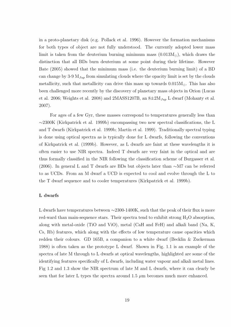
L dwarfs
L dwarfs have temperatures between ∼2300-1400K, such that the peak of their flux is more
red-ward than main-sequence stars. Their spectra tend to exhibit strong H2O absorption,
along with metal-oxide (TiO and ViO), metal (CaH and FeH) and alkali band (Na, K,
Cs, Rb) features, which along with the effects of low temperature cause opacities which
redden their colours. GD 165B, a companion to a white dwarf (Becklin & Zuckerman
1988) is often taken as the prototype L dwarf. Shown in Fig. 1.1 is an example of the
spectra of late M through to L dwarfs at optical wavelengths, highlighted are some of the
identifying features specifically of L dwarfs, including water vapour and alkali metal lines.
Fig 1.2 and 1.3 show the NIR spectrum of late M and L dwarfs, where it can clearly be
seen that for later L types the spectra around 1.5 µm becomes much more enhanced.
19

Figure 1.1: Optical spectra of an M9, L3 and L8 type, showing water vapour and alkali
metal features from Kirkpatrick et al. (1999).
20

1 1.5 2 2.50
2
4
6 LP 475-855 M7
LP412-31 M8
2M0345 L0
2M0746 L0.5
2M0829 L2
2M1029 L2
Figure 1.2: NIR spectra of M7-L2 dwarfs from Reid et al. (2001). The shaded regions
show areas affected by terrestrial water vapour absorption. Refer to Figs. 1.1 and 1.4 for
spectral features.
1 1.5 2 2.50
1
2
3
4
5
2M0036 L3.5
2M1112 L4.5
D0205 L7
2M0825 L7.5
2M0310 L8
Figure 1.3: NIR spectra of L3.5-L8 dwarfs from Reid et al. (2001). The shaded regions
show areas affected by terrestrial water vapour absorption. Refer to Figs. 1.1 and 1.4 for
spectral features.
21
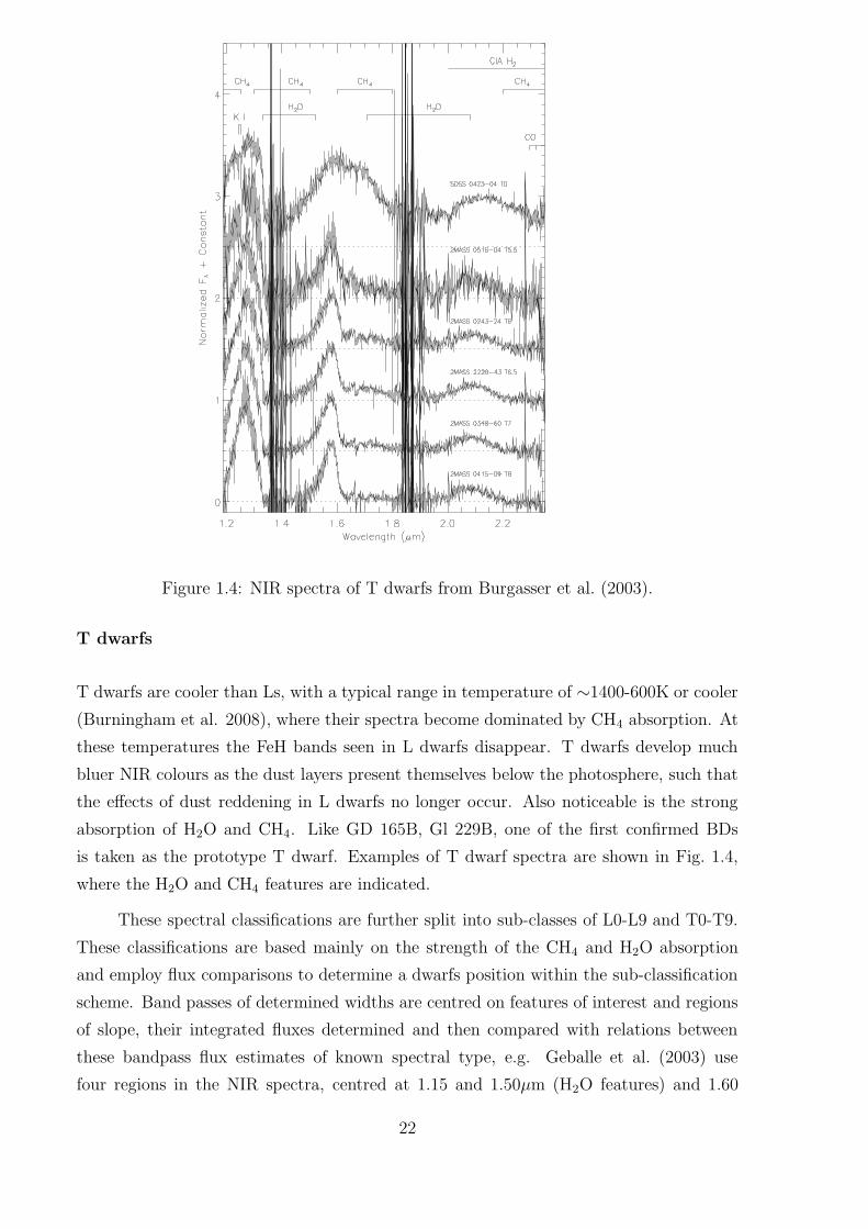
Figure 1.4: NIR spectra of T dwarfs from Burgasser et al. (2003).
T dwarfs
T dwarfs are cooler than Ls, with a typical range in temperature of ∼1400-600K or cooler
(Burningham et al. 2008), where their spectra become dominated by CH4 absorption. At
these temperatures the FeH bands seen in L dwarfs disappear. T dwarfs develop much
bluer NIR colours as the dust layers present themselves below the photosphere, such that
the effects of dust reddening in L dwarfs no longer occur. Also noticeable is the strong
absorption of H2O and CH4. Like GD 165B, Gl 229B, one of the first confirmed BDs
is taken as the prototype T dwarf. Examples of T dwarf spectra are shown in Fig. 1.4,
where the H2O and CH4 features are indicated.
These spectral classifications are further split into sub-classes of L0-L9 and T0-T9.
These classifications are based mainly on the strength of the CH4 and H2O absorption
and employ flux comparisons to determine a dwarfs position within the sub-classification
scheme. Band passes of determined widths are centred on features of interest and regions
of slope, their integrated fluxes determined and then compared with relations between
these bandpass flux estimates of known spectral type, e.g. Geballe et al. (2003) use
four regions in the NIR spectra, centred at 1.15 and 1.50µm (H2O features) and 1.60
22

and 2.20µm (CH4 features). More recently other features such as FeH are also used to
generate more accurate relations within the L and T sub-classes (Slesnick, Hillenbrand &
Carpenter 2004). Another method is to use the equivalent widths of the potassium lines
at ∼1.18µm (Reid et al. 2001a). For the very late T dwarfs that are now being discovered
(ULAS J0034-0052 Warren et al. 2007 and CFBDS J005910.90-011401.3 Delorme et al.
2008) a further spectral class beyond T will be needed. Pre-emptively coined ′Y-dwarfs′
by Kirkpatrick et al. (1999b) they are expected to be characteristically different from T
dwarfs. Such changes may result from the emergence of ammonia absorption in the NIR,
or effects due to the condensation of water clouds at ∼400K (similar to those seen in
Jupiter).
1.2 Benchmark ultracool dwarfs
There is no official criteria for what constitutes a benchmark UCD in the literature, other
than the fact that it has some known properties. In the context of this thesis however,
benchmark UCDs are those that have a known age. This parameter is vitally important
for the understanding of UCD properties and how they evolve with time. Currently it is
not possible to calculate the age of an isolated UCD in the field (with the exception of very
young objects that show lithium in their spectra) as models are not yet robust enough for
this prediction. Benchmark UCDs are thus vital to the calibration of such models and are
likely to be the testbeds for interpreting UCD atmospheric effects, which could lead to
the accurate prediction of physical properties from observable characteristics. Potentially
a UCD with an indicated age constraint is likely to be useful, when considering overall
trends. These are discussed in the later chapters of this thesis, where all known UCDs
with an age estimate are presented. However, if the age of the UCD is not very accurate
then the associated properties may not be particularly useful for calibrating models. The
ideal benchmark UCD should have an age accurate to 10% (Pinfield et al. 2006). These
benchmarks are the subject of the searches in this thesis. Where such benchmarks may
be found, as well as the application for the use of such benchmarks are described in the
following sections.
23

1.2.1 Ultracool formation scenarios
The formation of UCDs is still not well understood, but it is likely that they form initially
like stars (core collapse and accretion) but never acquire enough mass to ignite stable
hydrogen burning, only burning deuterium for a limited period of time, such that their
formation may take a slightly different course to those of normal stars. Briefly described
here are the four main types of theorised formation mechanisms, these include formation
by turbulent fragmentation, disc fragmentation, photo-erosion and ejection.
Turbulent Fragmentation
Formation of UCDs via turbulent fragmentation was first proposed by Padoan & Nordlund
(2002), who suggested that very low-mass cores could be formed during the process of
fragmentation in a turbulent cloud, which would then go on to produce very low-mass
objects. Their simulations show that turbulent flows commonly gives rise to variations
in the mass density distribution allowing substellar mass cores to be dense enough to
collapse and form UCDs.
Disk Fragmentation
It may also be possible for UCDs to form from initially massive prestellar cores via frag-
mentation of a large circumstellar disk (Bate, Bonnell & Bromm 2003). Whitworth &
Goodwin (2005) state that this theory could be possible for large disks (∼1000AU) where
the separation between the two components is relatively large (≥100AU), but would not
work for stars with smaller disks, where the temperature and surface density are higher,
such that the photo-fragments (small forming cores) are unable to cool fast enough to
condense out to form a UCD in the disk. This formation mechanism may also explain the′brown dwarf desert′ (the observed trend where UCDs are not found at separations of <
5AU from a main-sequence star binary companion Grether & Lineweaver 2006) as UCDs
formed in this fashion must have large separations. Whitworth & Stamatellos (2006) also
support this theory of formation but suggest that a massive enough circumstellar disk is
likely to be rare and short-lived, converting into UCDs quickly on a dynamical timescale
of only ∼104yr.
24

Ejection
The theory of UCD formation through embryo ejection or liberation was first suggested
by Reipurth & Clarke (2001). They postulated that UCDs form from prestellar cores
that are ejected from dynamically interacting multiple systems before they have had
time to accrete enough mass to ignite hydrogen. UCDs formed in this manner would
exhibit no kinematic imprint and are likely to be found as isolated objects, as shown in
the simulations of Bate et al. (see http://www.ukaff.ac.uk/starcluster). This formation
mechanism also requires a large amount of initial formation by fragmentation and core
collapse to produce the protostellar embryo that is ejected from the system. It cannot
however explain the large number of close UCD binaries that have been observed (Pinfield
et al. 2003).
Photo-erosion
The fourth formation mechanism is the theory of photo-erosion, whereby UCDs form in
the presence of a higher mass star embedded in a HII region. The higher mass object
causes compression waves and an ionisation front that photo-erodes surrounding low mass
cores. This theory produces UCDs for a wide range of initial conditions and predicts close
UCD binaries. However, the process is inefficient as it requires a massive protostellar core
to be eroded to form a single UCD, and can only work in the presence of an OB type star
to produce the high levels of UV needed for this formation mechanism to work (Whitworth
& Goodwin 2005).
None of the methods outlined here can, by themselves predict all the observed
dynamics of UCDs (the numbers of isolated and both close and wide binary systems) and it
seems likely that a combination of these mechanisms is responsible for at least some of the
UCDs discovered to date, possibly being dependent on environment, epoch and metallicity,
as reflected by collective UCD properties that are seen by observations. Indeed Goodwin
& Whitworth (2007) favour a combination of formation scenarios, suggesting that UCDs
are initially binary companions formed by gravitational fragmentation of the outer parts
(R > 100 AU) of the protostellar disc of a low-mass hydrogen-burning star. These are
then gently disrupted by passing stars, rather than violent interaction as suggested by
Reipurth & Clarke (2001). UCDs formed in this way would have velocity dispersions
and spatial distributions similar to that of higher-mass stars and they would likely be
able to retain discs and sustain accretion and outflows. This also implies that most stars
25

and UCDs should form in binary or multiple systems, which is supported by observations
(Pinfield et al. 2003), thus studies of UCDs in binaries could potentially be revealing
about their formation mechanisms.
1.3 The ultracool IMF and birthrate
To fully understand the nature of UCDs (other than the treatment of dust) and their
contribution to the galaxy, there are several important factors that need to be understood
in order to answer these questions. How do they form? at what rate does this happen?
how do they evolve? and what is their contribution to the very low mass end of the mass
function (MF) and the initial mass functions (IMF)? The current knowledge on these
factors are briefly outlined below.
1.3.1 The substellar initial mass function
The IMF describes the distribution of newly formed stars as a function of mass, which
can be described as a power law of the form M−α. Salpeter (1955) showed that α=2.35
for stars equal to or larger than M�, this is referred to as the Salpeter function and states
that the number of stars of each mass range decreases with increasing mass. This form of
the IMF stays fairly uniform regardless of environment for stars M>M�. Miller & Scalo
(1979) and Scalo (1986) expanded on this work for stars < M�, suggesting that the IMF
flattens for lower masses where α=0 for stars below M�, as shown in Fig. 1.5. Kroupa
(2001) however suggests that α=2.3 to half a solar mass but then reduces to α=1.3 for
masses 0.5<M�<0.08 and to α=0.3 below 0.08M�. Traditionally the IMF is estimated
from a luminosity function and a mass-luminosity relation, this is a problem however
for UCDs, as the initial heat from gravitational contraction is slowly radiated away with
time, such that the UCD mass-luminosity relation is a factor of age. Currently neither the
mass, nor the age can be calculated from luminosity alone, making it difficult to calculate
an IMF for field UCDs, as a history of the star formation along with an accurate age is
needed. This was attempted by Reid et al. (1999), who calculated an IMF for stars in
the solar neighbourhood from 2MASS and showed evidence for a substellar IMF that is
shallower than the Salpeter IMF. However the models they use (Burrows et al. 1997b) are
geared towards dust-free atmospheres and do not represent the characteristics of dustier
26

Figure 1.5: The present day mass function of main-sequence field stars from Miller &
Scalo (1979), where the MF φms(log M) as the number of stars (pc−2logM).
L dwarfs. Allen et al. (2005) took a slightly different approach and calculated the IMF
for M<0.08M� to be in the range -0.6< α <0.6 using Bayesian techniques.
The problems associated with determining the IMF for field UCDs could poten-
tially be solved by determining the ages of UCDs and obtaining theoretical masses using
evolutionary models. This may be done by observing open cluster populations where
stars and UCDs of different masses with well defined ages would be abundant. There are
however potential difficulties when observing objects in clusters such as sources of extinc-
tion, uncertainties in age and distance, and contamination from non-members. Studies of
young clusters have been performed by Andersen et al. (2008) who looked at the IMF in
young clusters including IC348, where Luhman et al. (2003b) found that the IMF rises
as a Salpeter function from high/intermediate masses down to ∼M� and then rises more
slowly to a mass around M=0.1-0.2M�, turning over and declining into the substellar
regime. They also looked at the IMF in Taurus (Briceno et al. 2002, Luhman et al.
2003a) and find that it appears to rise quickly to a peak of ∼0.8M� and then steadily
declines to lower masses. The trend of a falling mass function in the ultracool regime
is generally shared with the observations in other clusters (Chameleon1; Luhman 2007,
Pleiades; Lodieu et al. 2007a; Chabrier 2003; Moraux et al. 2003, Orion; Hillenbrand
1997; Luhman et al. 2000; Muench et al. 2002 and NGC2024; Levine et al. 2006) as can
be seen in Fig. 1.6, showing the MF of the Pleiades (Lodieu et al. 2007a). The different
27

forms of the IMF in these clusters all show subtle differences, suggesting that they might
be sensitive to initial condition. These differences however, may also be able to help pin
down the formation mechanisms for UCDs.
The recent simulations and studies of late T dwarfs (>T4) in the field from the
UKIDSS LAS by Pinfield et al. (2008) suggest that a log normal form of the MF agrees
best with both their observations and observations of clusters (e.g. Pleiades MF from
Chabrier 2003; Lodieu et al. 2007a). The slope of the function appears to steepen,
increasing as mass decreases, suggesting a function that is consistent with an α=0 power
law around a mass of ∼0.04M�. This would also suggest that as T dwarfs probe lower
mass ranges, the mass function may differ for L dwarfs from that of T dwarfs and that
T dwarfs may be more sensitive to changes in the IMF, as shown by the simulations of
Allen et al. (2005) in Fig. 1.7. The findings of Pinfield et al. (2008) indicate that for the
field population the substellar MF is most consistent with an α=-1.0 and α=0.0 for L and
T dwarf populations, respectively.
1.3.2 The substellar birth rate
The birth rate is the number density of stars born per unit time and determines the MF
and IMF. For main-sequence stars the MF is thought to stay constant with time (Miller &
Scalo 1979) but remains undefined for substellar objects. Burgasser (2004) made Monte
Carlo simulations of five UCD birth rate scenarios, including a constant birth rate (flat),
similar to that taken for galactic star formation, an exponential birth rate, such that the
star formation rate scales with average gas density. They also consider an empirical birth
rate in the form of a series of star formation bursts, which would agree with the apparent
increase in star formation ∼400 Myr ago (Barry 1988). A fourth scenario is a stochastic
birth rate, where star formation occurs only in young clusters and only for a series of short-
lived bursts, producing an equal amount of UCDs at each event. Finally they consider a
halo birth rate where only UCDs born over a 1 Gyr range, occurring 9 Gyr ago and that
represent the halo population. These five scenarios are all compared for α=0.5, where
they shows that there is little difference between the majority of scenarios and that only
the extreme exponential and halo birth rates show any strong dissimilarities, as these
scenarios produce a larger number of older, more evolved UCDs. They also suggest that
UCDs in the Teff range 1200-2000K (L and early T dwarfs) may be more sensitive to the
birth rate than later type T dwarfs, as shown by Fig. 1.8. Using a number of late T dwarfs
28
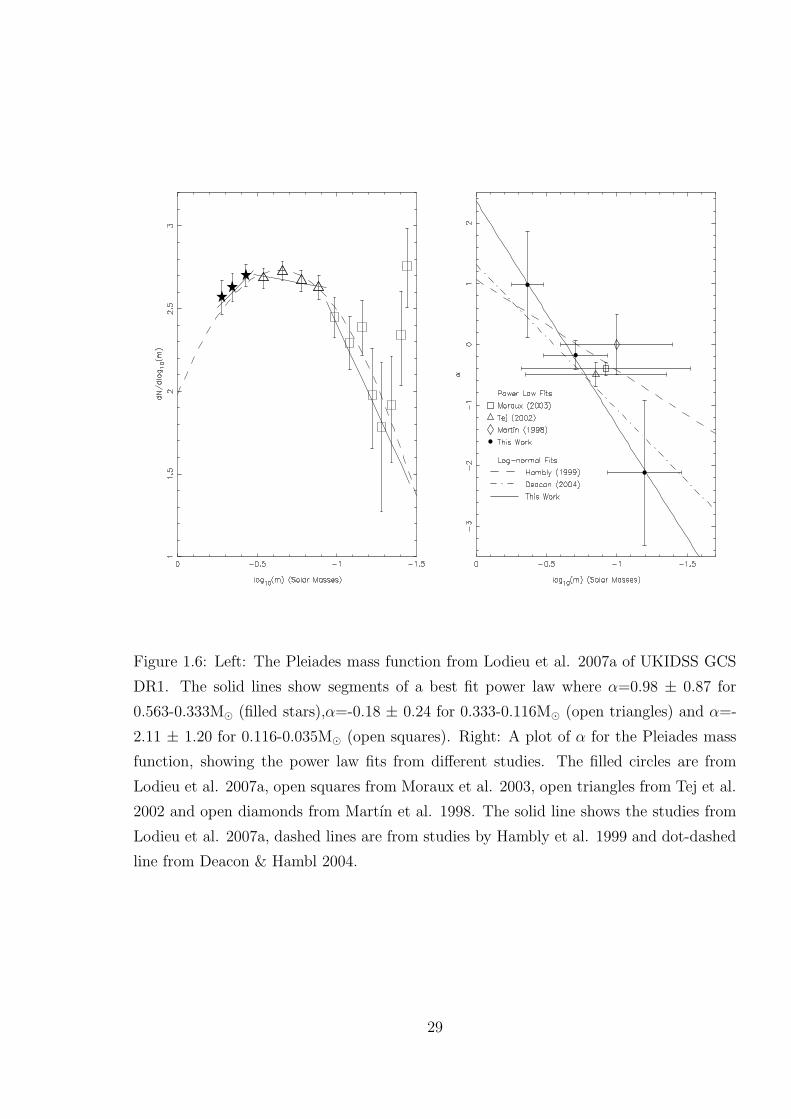
Figure 1.6: Left: The Pleiades mass function from Lodieu et al. 2007a of UKIDSS GCS
DR1. The solid lines show segments of a best fit power law where α=0.98 ± 0.87 for
0.563-0.333M� (filled stars),α=-0.18 ± 0.24 for 0.333-0.116M� (open triangles) and α=-
2.11 ± 1.20 for 0.116-0.035M� (open squares). Right: A plot of α for the Pleiades mass
function, showing the power law fits from different studies. The filled circles are from
Lodieu et al. 2007a, open squares from Moraux et al. 2003, open triangles from Tej et al.
2002 and open diamonds from Martın et al. 1998. The solid line shows the studies from
Lodieu et al. 2007a, dashed lines are from studies by Hambly et al. 1999 and dot-dashed
line from Deacon & Hambl 2004.
29

Figure 1.7: Three bolometric luminosity functions from Allen et al. (2005) comparing
models of α = 0.0 (solid line), 0.5 (dotted line) and 1.0 (dot-dashed line) for M, L and T
dwarfs.
discovered from the UKIDSS LAS, Pinfield et al. (2008) suggest from observations that
an IMF of the form α≥0 is unlikely and favour a range of -1.0<α<-0.5. Analysis of a
larger sample of L and early T dwarfs, over short Teff=100K bins in the range 1100-1500K,
would be able to rule out at least extreme scenarios (e.g. exponential or halo birth rates).
1.3.3 Ultracool evolution
BDs and UCDs are not massive enough to burn hydrogen, but instead burn deuterium
for some fraction of their lifetime. For the most massive UCDs this can be as short as
10Myr, at which point deuterium burning within the core will cease and the UCD will
be supported by electron degeneracy pressure. They then simply cool and radiate away
their internal thermal energy. Fig. 1.9 shows the cooling tracks for low-mass stars, brown
dwarfs and exoplanets, taken from Burrows et al. (1997a). UCDs have masses between
those of low-mass stars and exoplanets and as a result their cooling tracks appear like
a mixture of the two cases. The kinks in the tracks for the higher mass objects relate
to the switch-off of deuterium burning in the particular type of object. It is clear that
30

Figure 1.8: Comparison of Φ(Teff) for α=0.5 for different birth rate scenarios from Bur-
gasser et al. (2004) as disussed in the text. These include a flat/constant (solid black line),
exponential (gray solid line), empirial (black dtted line), a stocastic/cluster (gray dotted
line) and a halo (black dashed line) birth rate. The constant, empirical and cluster birth
rates show nearly identical distribuations, where as the exponential and halo distributions
show significant variations in the Teff range 1200-2000 K.
UCDs and stars differ in the region where this occurs but UCDs unlike stars continue
cooling indefinitely, similar to exoplanets. Throughout this cooling time the UCD will
evolve through the L sequence to the T sequence and to cooler temperatures over billions
of years. This means that very old UCDs are difficult to image as they are intrinsically
fainter than their younger field counterparts.
1.4 Understanding and interpretation of ultracool at-
mospheres
One of the most notable characteristics of UCDs from the observation of their spectra
and photometry is that dust grains composed of Al2O3 (corundum), MgSiO3, CaSiO3,
VO, TiO and other metal oxides and silicates can form and condensate out in their upper
atmospheres. The cool temperatures of UCDs provide the right environment for heavier
elements to form in their atmospheres, thus allowing more complex chemistry to occur,
similar to that seen in the gas giant planets like Jupiter. This has profound effects on
the observable characteristics of UCDs, causing large changes in their colours and the
31

Figure 1.9: Cooling tracks for brown dwarfs, stars and planets taken from Burrows et
al. (1997).
emergence of features such as water vapour and methane in their spectra. The key to
understanding the changes within the spectra of these cool, substellar objects lies in the
understanding of their complex atmospheres and how dust affects not only their physical
but observable characteristics.
1.4.1 Atmospheric models
The spectra of UCDs are dictated by their atmospheric physics and properties, and a
proper understanding thereof should thus allow accurate predictions of UCD properties
and ultimately their evolutionary behaviour. Several models have been produced that try
to explain the changes in the spectral and photometric characteristics that are observed
for L and T dwarfs and to explain what happens at the transition between the two
subclasses. These models can have very different effects on the resulting spectra and
colours, depending on how they treat dust in the atmosphere (e.g. the amount of dust,
grain size and composition). Traditionally stellar modelling relied on gray models that
lacked any inclusion of dust, but clearly this is not the case for UCDs, where dust plays
a significant role in the underlying physics, shaping their appearance.
32

Lyon (Phoenix) group models
The NextGen models (Baraffe et al. 1998) were some of the first models produced to try
and physically describe the appearance of UCDs, they do not include dust grains, but take
into account opacities, however they tend only to be useful for Teff>1700K. The latest
results from the Lyon group present two model scenarios, one to explain the hotter, redder
L dwarfs, known as the DUSTY models (Chabrier et al. 2000a; Baraffe et al. 2002) and
the COND (condensate) models (Allard et al. 2001; Baraffe et al. 2003) that try to explain
the cooler, bluer T dwarfs (both models are for solar metallicity scenarios). The models
use mixtures of several hundred gas and liquid species and opacities of more than 30 types
of sub-micron sized dust grains, including Aluminium, Magnesium and Calcium silicates.
For this they assume that dust forms in equilibrium with the gas phase. The DUSTY
models are applied to temperatures ∼3000-1400K and log g=3.5-6.0 and take into account
both the formation and opacity caused by dust grains. They describe reasonably well the
NIR colours and spectra of early-mid L dwarfs, where Teff>1800K but the predicted optical
colours show discrepancies from observations on the order of 0.2-0.3 mags. The COND
models take into account the formation of dust but no effects of atmopheric opacity,
representing the dust-free appearance and general bluer colours of T dwarfs. This model
is presented for Teff from 3000-700K and log g=2.5-6.0. The properties of UCDs with
Teff≤1300K are better described by the COND models than the DUSTY models. These
models both struggle to reproduce observations seen at the transition between late L to
early T dwarfs, suggesting that at this stage dust seen in the photosphere of L dwarfs
primarily forms lower in the atmosphere of T dwarfs, and gravitationally settles below the
photosphere, with the observed atmosphere being relatively dust-free. They state that
these models used together represent extremes that might be expected in the properties
of UCDs.
AMES models
The AMES group (Marley et al. 2002; Saumon et al. 2003) produced models using a
self-consistent treatment of cloud formation. They suggest that i − z colour is extremely
sensitive to chemical equilibrium assumptions, having an affect of up to ∼2 mags on
colour. They consider not only the sedimentation of condensates but also the efficiency
of the process to help explain both L and T dwarfs and the L/T transition with the
same model, for solar metallicity. As such they attempt to represent an intermediate
33

between the DUSTY and COND extremes. In this case the cloud decks are confined to a
fraction of the pressure scale height and the models assume that it is sedimentation that
controls vertical mixing in the clouds, causing the observed turnover in J −K colour with
decreasing Teff . They also take into account grain sizes between 10-100µm and assume
that if the grain size is less than the observed wavelength of light, Rayleigh scattering
dominates and has little affect on opacity. The problems with this model are that while it
predicts the overall trend seen by observations, the finer details are not matched, e.g. the
peak of the model value in J − K is not as red as that observed, and the models predict
a move to bluer colours that is much slower than is actually observed.
Tsuji models
The models of Tsuji, Nakajima & Yanagisawa (2004) use an empirical unified cloud model
for cases of log g=4.5-5.5, where they assume the dust column density is relative to that
of the gas column density in the photosphere for this range of log g. Their initial models
assumed that dust forms everywhere, as long as the thermodynamic conditions are right
for condensation (Tsuji, Ohnaka & Aoki 1996). However this was only good for predicting
the colours of late M and early L dwarfs. Their latest models include the segregation of
dust from gaseous mixing at a corresponding critical temperature (TCR; related to the
temperature of condensation). Dust then remains in the photosphere of warm dwarfs
where Teff>TCR is optically thick. In cooler dwarfs where Teff<TCR, producing an optically
thin region and the dust is segregated and precipitated. This model represents the L/T
transition reasonably well on a colour-magnitude diagram and from spectra, however the
detailed behaviour does not match observations (e.g. see the J −K, MJ diagram in Tsuji
& Nakajima 2003).
Tuscon models
Burrows, Sudarsky & Hubeny (2006) use a model of refractory clouds, coupled with the
latest gas-phase molecular opacities for dust molecules, similar to those used by the Lyon
group. They also look at the effects of gravity and metallicity and vary grain size, cloud
scale height and cloud distribution, applicable over a Teff=2200-700K range. They show
generally good agreement with the observed spectra of NIR colours for early-mid L and
mid-late T dwarfs and by varying gravity parameters get a closer fit to the L/T transition
than other models. However they do not reproduce the apparent brightening seen in the
34
J- band at the transition, nor the dimming at very late T. They suggest that the L/T
transition is likely related to gravity and possibly metallicity but needs better explanation.
As yet no self-consistent model has been presented that can reproduce the observed
characteristics of L and T dwarfs and how they evolve from one type to the other consis-
tently in both optical and NIR colours and spectra. It seems evident that the treatment of
dust plays a vital part in fully understanding the underlying physical processes at work.
Also the affects of gravity and metallicity are largely ignored by the models, with the
exception of the latest Burrows models and may also play a significant role.
1.4.2 Benchmark UCDs as members of binary systems
What is needed to help the models explain the characteristics being observed are bench-
mark UCDs, where the age and distance can be measured or determined without the
need to refer to synthetic spectra, which struggle to accurately predict true characteris-
tics. There are several ways in which benchmark UCDs could be found. Firstly young
(≤1 Gyr) benchmark objects could be found as members of clusters and moving groups,
where UCDs associated with a cluster (through shared kinematic properties) have a well
constrained age and a known metallicity. Very young clusters, e.g. the Orion nebula
cluster also provide the nursery environments, where UCD formation and the properties
of very young UCDs can be studied. The distance to which these young benchmarks can
be observed is generally larger than that of field UCDs, as they are much brighter at these
very young (∼1Myr) ages. However for the older, more evolved population it is somewhat
more difficult to constrain the age, as this can not, in general be done for isolated field
UCDs. The best source of benchmark objects comes from UCDs as members of binary
systems, where the age can be inferred from the primary component, as members of bi-
nary systems are expected to have formed from the same nascent cloud. Of particular use
are eclipsing binaries where the mass and radius can be calculated from the dynamics of
the system, though depending on the parent star it may be difficult to measure the age
accurately.
The ideal primary for a binary system containing a UCD, would be a star whose age
can be accurately constrained, in particular binaries can be discovered in large numbers
from photometric surveys, e.g. SuperCOSMOS, SDSS, 2MASS and UKIDSS (described
in Chapter 2). Wide binaries with a separation >1000 AU are known to be quite common
around main-sequence stars. Gizis et al. (2001) found an L-dwarf companion fraction
35

Figure 1.10: Hertzsprung-Russell diagram showing the evolution for a solar type star
(www.skyserver.sdss.org).
of 1.5%, from which a UCD companion fraction of 18±14% was calculated. However,
they only used a sample of three L dwarf companions to main-sequence stars to infer this
fraction. Pinfield et al. (2006) on the other hand find a larger L dwarf companion fraction
of 2.7+0.7−0.5%, using a larger sample of 14 common proper motion companions to Hipparcos
stars out to a limiting magnitude of J = 16.1, which a wide companion UCD fraction
of 34+9−6% is inferred, assuming the fraction of UCDs detected as L dwarfs is =0.08 (the
companion MF for an α=1 from Gizis et al. 2001). Thus wide companion UCDs to main-
sequence stars should be sufficiently numerous to provide a useful population for study.
The problem with main-sequence stars however is that their ages can be largely uncertain.
The later stages of stellar evolution however may prove more reliable age indicators, for
example the subgiant phase is very short compared to the MS lifetime and the age of a
star in this phase can be fairly well constrained. The white dwarf (WD) phase is also well
understood and the cooling age of a WD can be accurately measured, along with the age
of the progenitor that can be accuratly calculated from models.
36

1.4.3 Stellar evolution beyond the main-sequence
Subgiants
Stars of mass 0.8≤M�≤8.0 spends the majority of their lifetime on the main-sequence
of the Hertsrung-Russell diagram (HR; as shown in Fig. 1.10). Once a star has used
up all of its fuel, it ceases to fuse hydrogen in its core, causing the core to contract,
increasing the stars central temperature enough to cause hydrogen fusion to occur in the
a shell of hydrogen surrounding the core, which is now helium rich. The star starts to
expand, increasing both in diameter and in brightness. However the star’s temperature
and colours stay relatively consistant with its main-sequence counterpart. At this point
the star leaves the main-sequence and evolves rapidly, moving horizontally across the
HR diagram before joining the base of the red giant branch. The time it occupies this
phase is very brief and with comparison to evolutionary models, its age can be accurately
determined. During this point of the stars evolution it has not undergone any mixing or′dredging up′ of materials, where the outer convective layers start to penetrate the inner
layers, mixing materials formed closer to the core and bringing them from the lower layers
up to the surface. This would wipe out any original metallicity information, as the star
would make its way to the giant phase.
As subgiants have not yet undergone this dredge-up phase their metallicity can still
be accurately measured by comparisons with evolutionary models. Theoretical predictions
of subgiant evolution are sensitive to metallicity, where the largest uncertanties arise
from the extent of convective core overshooting (Roxburgh 1989) that occurs for different
masses. This uncertainty is yielding to accurate observational constraints via the study
of different aged open clusters (e.g. VandenBerg & Stetson 2004). UCD companions to
subgiants have been previously identified by Wilson et al. (2001), who confirmed an L
dwarf companion to an F7IV-V star primary from 2MASS. They find that subgiants give
better age constraints (±30 %) compared to F dwarf main-sequence stars (from their
fig. 4.). This subgiant has only just left the main-sequence, but fully fledged subgiants
are likely to have better age constraints. Indeed subgiants with accurately measured
metallicity [Fe/H] accurate to 0.1 dex (Ibukiyama & Arimoto 2002) and either a distance
known to within 5% or log g to 0.1 dex could allow the subgiant age to be constrained
to within 10% accuracy (Thoren, Edvardsson & Gustafsson 2004), making them excellent
age calibrators. Such UCD companions to subgiants will have an accurate measurable
metallicity as well as age. Teff and log g could also then be measured, giving a UCD with
37

well defined properties.
The red giant and asymptotic giant phases
As the star evolves along the red giant branch, slowly burning the hydrogen in the shell
around the helium rich core, the star continues to increase expanding rapidly. The surface
temperature of the star then decreases as the star has expanded. When the temperature
decreases lower than 5000 K dredge up can occur. During this time the helium core
contracts and the internal temperature increases. When it has contracted so much that it
is now gravitationally suported by electron degeneracy pressure. As the pressure suporting
the star is no longer dependent on temperature the core continues to generate energy and
increase heating in a run-away situation, known as the helium flash. Burning of helium
then takes place in the core. Once most of the helium has been converted to carbon and
oxygen in the core, a shell of helium and hydrogen around it is produced. The star again
expands to become a red giant once more, with a radius comparable to 1 astronomical
unit. At this point the star leaves the red giant branch and joins the lower part of the
asymptotic giant branch (ABG). The star again increases in temperature and luminosity,
moving back towards the left hand side of the main-sequence. After the helium shell has
run out of fuel the star cools but increases in luminosity and its main source of energy
production is shell hydrogen burning around the inert helium shell. Over a very short
period (10,000-100,000 yr) the helium shell can ’switch on’ again and the hydrogen shell
burning switches off, creating another helium flash or thermal pulse. Several of these,
on short timescales can occur, causing additional dregde-up of materials. The increased
luminosity results in high radiation pressure, causing a strong stellar wind. Eventually the
star looses most of its envelope and shrinks with constant luminosity. The temperature
increases to 108K and the circumstellar envelope becomes visible as a planetary nebula.
Near the hottest point of this post-AGB evolution the nuclear energy generation ceases
and it remains a hot WD with a Carbon-Oxygen core, surounded by layers of hydrogen
and helium (Prialnik 2000; Boehm-Vitense 1992).
38

White dwarfs
When the star looses the majority of mass, during the planetray nebula phase, it does so
at a random phase of the thermal pulse cycle. For the majority of stars this occurs during
the hydrogen buring phase, which occurs for a longer period of time than helium burning.
The star is thus left with a thin layer of helium and an outer layer of hydrogen and exhibits
strong hydrogen lines in its spectrum, and is classified as a DA WD. However if the star
undergoes a helium flash after leaving the AGB phase then it will be left with a helium
layer, stripping away the hydrogen. These helium atmosphere WDs show helium lines
in their spectra, however the majority (∼85%; Althaus et al. 2009) of WDs form with
hydrogen atmospheres. The remaining WDs have predominatly helium atmospheres, and
are classified by their atmospheric content. The most basic helium rich WD just shows
helium lines in its spectra and no hydrogen line, this type of DB WD has temperatures
between 12,000-30,000 K. The helium can also be in an ionised form (a DO WD) if it is hot
enough, having a temperature in the range 45,000-100,000 K. Helium atmosphere white
dwarfs with temperatures cooler than 12,000 K however, will have a featureless spectrum
(a DC WD). It is also possible to see additional metal lines in the WD atmosphere (DZ
white dwarfs), however the reasons for this are not fully understood. It has been sugested
that these could be the result of circumstellar disks (Farihi, Zuckerman & Becklin 2008).
There is also a very small fraction (0.1%) of white dwarfs that have carbon atmospheres
(DQ WD), which are thought also to have formed if the WD undergoes a very late thermal
pulse during the early stages of cooling, where it re-enters the WD stage in a ’born-again’
phase. Gravitational settling is thought to cause the star to go from a helium rich DO
into a DB and then DQ as it cools and carbon difuses up from the core (Dufour et al.
2008). Table. 1.1 show the characteristics of the different spectral types of WDs from
Sion et al. (1983). The different phases from the main-sequence are illustrated in the HR
diagram in Fig. 1.10.
White dwarf maximum mass and evolution
The WD itself has no nuclear energy source so the energy it radiates at its surface comes
from thermal energy stored in ions that is supported by pressure from degenerate electrons.
These degenerate electrons are in the form of a gas in the WD which is homogeneous and
isothermal. As the density and pressure increase within the WD, the degenerate gas
becomes relativistic. The maximum mass of a WD is set by the mass-radius relation that
39

Table 1.1: The classification scheme for WDs from Sion et al. (1983).
Type Spectral Features
DA Shows strong hydrogen (HI) lines.
DB Shows strong neutral Helium (HeI) & no HI lines.
DO Shows ionised Helium (HeII) lines.
DC Shows a continuous spectra.
DZ Shows strong metal lines & no Hi,HeI/HeII or Carbon lines.
DQ Shows strong atomic or molecular carbon (C) lines.
DX Has a peculiar or unclassifiable spectra.
was first defined by (Chandrasekhar 1931) and means that a WD of mass >1.4M� can
not be supported against gravity. This also means that as the mass increases the physical
size of a WD must decrease.
The mass-radius relation can also be used to relate the luminosity to mass. As
luminosity depends upon surface temperature and radius, this implies that as a WD cools
it simply fades, evolving along a specific track as illustrated by the evolutionary models
of Chabrier et al. (2000b), shown in Fig. 1.11. High mass WDs (≥0.65M�) will have
relatively high mass main-sequence progenitors, which would have had a relatively short
main-sequence lifetime (using initial-final-mass relations [IFMR], e.g. Dobbie et al. 2006
and main-sequence lifetime estimates) and the total age of the WD will essentially be the
same as the cooling age of the WD. Lower mass WDs come from lower mass main-sequence
progenitors, where the main-sequence lifetime is less accurately known and could be up to
∼10 Gyr old, with a minimum age likely greater than 1 Gyr, for an average main-sequence
star in the field. Hot WD atmospheres of pure hydrogen can be well modelled (Hubeny &
Lanz 1995) to constrain Teff and log g from accurately fitting synthetic spectra to Balmer
lines in the optical (Claver et al. 2001; Dobbie et al. 2005), such that WD cooling ages
can be determined from Teff and log g (assuming a mass-radius relation) and evolutionary
models. Thus higher mass WDs are more desirable for constraining the ages of UCD
companions, as illustrated by the IFMR shown in Fig. 1.12. It is not possible however,
to establish the metallicity of the WD progenitor from observations since the surface
composition of the WD is not representative of its main-sequence progenitor composition.
40

Figure 1.11: Cooling tracks for DA WDs of different mass from Chabrier et al. (2000).
Figure 1.12: The initial-final-mass-relation from Dobbie et al. (2006) for Hyades WDs
(open triangles), Praesepe (black circles), M35 (open diamonds), NGC2516 (open crosses)
and the Pleiades (open stars). Linear fit to the data is shown by the solid line (fit to
CO core), dashed line (fit to C core) and the relations of (Weidemann 2000) (dotted)
overplotted.
41

Previously identified white dwarf + ultracool dwarf systems
There have been several searches to find UCD companions to WDs. Despite this,
only a small number of detached UCD + WD binaries have been identified; GD 165B(L4
Zuckerman & Becklin 1992), GD 1400(L6/7; Farihi & Christopher 2004; Dobbie et al.
2005), WD0137 − 349(L8; Maxted et al. 2006; Burleigh et al. 2006a) and PG1234+482
(L0; Steele et al. 2007; Mullally et al. 2007). The two components in GD16 are separated
by 120AU and the separation of the components in GD1400 and PG1234 + 482 are
currently unknown, and WD0137 − 349 is a close binary (semi-major axis a = 0.65R�).
Farihi, Becklin & Zuckerman (2005) and Farihi, Hoard & Wachter (2006) also identified
three late M companions to WDs; WD2151 − 015 (M8 at 23AU), WD2351 − 335 (M8
at 2054AU) and WD1241 − 010 (M9 at 284AU). The widest system previously known
was an M8.5 dwarf in a triple system – a wide companion to the M4/WD binary LHS
4039 and LHS 4040 (Scholz et al. 2004), with a separation of 2200AU. There are several
other known UCD + WD binaries, however these are cataclysmic variables (e.g. SDSS
1035; Littlefair et al. 2006, SDSS1212; Burleigh et al. 2006b, Farihi, Burleigh & Hoard
2008, EF Eri; Howell, Nelson & Rappaport 2001) and are unlikely to provide the type of
information that will be useful as benchmarks, as they have either evolved to low masses
via mass transfer or their ages cannot be determined because of ongoing interaction. The
components of CVs are also not directly observable due to obsuration by the accretion
disk formed around the system.
Recent analysis from Farihi, Becklin & Zuckerman (2008) shows that the fraction of
L dwarf companions at separations within a few hundred AU of WDs is <0.6%. Despite
this, UCDs in wide binary systems are not uncommon (revealed through common proper
motion) around main-sequence stars at wider separations of 1000− 5000AU (Gizis et al.
2001; Pinfield et al. 2006). However, when a star sheds its envelope during the post-main-
sequence evolution, it may be expected that a UCD companion could migrate outwards
to even wider separation (Jeans 1924; Burleigh, Clarke & Hodgkin 2002) and UCD + WD
binaries could thus have separations of up to a few tens of thousands of AU. Although some
of the widest binaries may be dynamically broken apart quite rapidly by gravitational
interactions with neighbouring stars, some systems may survive, offering a significant
repository of benchmark UCDs.
42

1.5 Motivation and thesis structure
The aim of the work in this thesis is to uncover benchmark UCDs as members of binary
systems, where the primary member of the binary has a calibratable age. The UCDs
discovered will be able to aid the calibration of UCD properties, allowing models to be
refined, enabling them to reproduce observable properties with greater accuracy than is
currently possible. This thesis is split into six chapters outlining the main project com-
ponents I have worked on over the course of the Ph.D and are organised in the following
structure:
Chapter 2: Describes the techniques used to select UCDs and WDs from available
online data resources and catalogues, including the SuperCOSMOS, SDSS (for WDs)
and the 2MASS and UKIDSS (for UCDs) sky surveys, using a combination of colour,
magnitude and proper motion constraints. Presented here are the sets of candidate objects
that are searched for potential binary systems.
Chapter 3: Outlines the search for widely separated UCD companions to WDs,
including the results from a search of SuperCOSMOS and 2MASS for common proper
motion systems. One system is confirmed, spectroscopically and has been published (Day-
Jones et al. 2008), its properties and usefulness as a benchmark are also discussed. Also
presented are candidate systems from SDSS (DR6) and UKIDSS (DR3), and preliminary
follow-up for several of these systems, including a spectroscopic WD + M4 dwarf system
with a potential wide UCD companion.
Chapter 4: Describes a pilot NIR imaging survey of subgiant stars in the southern
hemisphere for widely separated UCD companions. Presented are the results from the
follow-up program and the candidate systems identified.
Chapter 5: Presents the confirmation of two UCD companions to main-sequence
stars, where their properties are derived and ages for the systems are calculated and
assessed for suitability as benchmark objects.
Chapter 6: Discusses the findings of the various searches for UCD companions
and compares them with other benchmark UCDs from the literature, where trends with
properties (temperature, gravity and metallicity) are explored as functions of observable
characteristics to assess current potential for the use of benchmark UCDs and highlight
useful future directions.
43

44

Chapter 2
Selection Techniques
Online data archives provide an easy and efficient way to access large amounts of data
that cover a wide area of sky and allow one to select objects of interest, such as WDs
and UCDs here. UCDs are well characterised by their colours, especially in the near
infrared (NIR), where surveys such as the 2 Micron All Sky Survey (2MASS; Skrutskie
et al. 2006) and the UK Infrared Deep Sky Survey (UKIDSS; Lawrence et al. 2007) are
particularly sensitive to such objects, as they are brightest at these wavelengths. These
surveys provide the largest and deepest search area available in the NIR to date, thus
providing an excellent way of selecting large numbers of stars and UCDs.
WDs can also be successfully selected via their colours and proper motions from
optical surveys such as the SuperCOSMOS Sky Survey and the Sloan Digital Sky Survey
(SDSS; Hambly, Digby & Oppenheimer 2005; Kleinman et al. 2004; Eisenstein et al.
2006), making them the ideal searching facilities for selecting WDs.
These surveys provide an invaluable tool for selecting candidate WDs and UCDs,
which could make up components of widely separated WD + UCD binaries. The tech-
niques used to select potential WD candidates from the SuperCOSMOS and the SDSS
surveys and UCD candidates from the 2MASS and UKIDSS sky surveys are described in
the following sections.
45

2.1 Selecting white dwarfs
2.1.1 White dwarfs in SuperCOSMOS
The online data archive SuperCOSMOS is a compilation of digitised sky survey plates
taken with the UK Schmidt and ESO Schmidt (in the south) and with the Palomar
Schmidt (in the north) telescopes. The database is accessed through the SuperCOSMOS
Science Archive (SSA); http://surveys.roe.ac.uk/ssa) where data can be obtained through
the use of Structured Query Language (SQL). Initially the SSA covered 5000 degrees2 of
sky, primarily covering the southern hemisphere from -60◦ to +3◦ DEC, in B-, I- and two
R- band epochs, with R- limiting magnitudes of 21.0 and 21.5, respectively. These two
epochs are taken using slightly different filters, the R59 and R63 filters, whose wavelength
coverage varies slightly from those of the Cousins R- band, but can be easily converted
using colour relations. As of August 2008 the survey is now complete and covers the
whole sky, however work presented here made use of the southern release only.
Candidate WDs were selected from the SSA, following a similar technique to that
of Knox, Hawkins & Hambly (1999). Candidates were selected based on their position
on a reduced proper motion (RPM) diagram, a technique that reduces the proper motion
to a linear velocity, such that reduced proper motion (in the R- band) is expressed as
HR = R + 5 log µ + 5, thus enabling it to be used as a proxy for absolute magnitude and
hence distance, taking advantage of the fact that nearby objects in general have higher
proper motion. WDs occupy a distinct region of the RPM diagram and have successfully
been selected via this method (Hambly, Digby & Oppenheimer 2005). Fig. 2.1 shows a
SuperCOSMOS RPM diagram with the location of WDs. An initial SSA sample (shown
as dots) was a magnitude selected sample (R ≤20) to avoid sources near the plate limit.
Potential candidates were also selected to be moving sources by requiring proper motion
(PM)≥10 mas/yr, PMσPM≥5 and to be stellar-like sources, requiring a database object to
have a class=2. In addition the galactic plane was avoided (requiring |b| ≥25◦) to minimise
confusion due to crowded fields, and SSA I- band coverage was also required (δ ≤+3◦),
which offers possible additional epochs for nearby UCD candidates (see §3.2.1). Quality
constraints on the database photometry were also imposed requiring the flag qual≤1040
in each of the B-, R- and I- bands ensuring that the object is unlikely to be a bright star
artifact. The main-sequence and WD sequence can be clearly seen in Fig. 2.1, and display
46

good separation for B − R ≤1.3. To further illustrate the location of the WD sequence,
overplotted are the positions of WDs from the spectroscopically confirmed McCook &
Sion WD catalogue (McCook & Sion 1999; here after MS99), along with pre-WDs (i.e.
sdO stars) and Halo objects from Leggett (1992). Also overplotted are subdwarf B stars,
hot, cool and extreme subdwarfs from Kilkenny, Heber & Drilling (1988), Stark & Wade
(2003), Yong & Lambert (2003) and Monet et al. (1992) respectively, which can have high
velocity dispersions and can masquerade as WDs in RPM diagrams. The overplotted
populations help confirm the location of the WD sequence for B − R ≤1.3 and allow the
location of WDs to be assessed out to redder colour. The final RPM selection criteria were
chosen to strike the best balance between WD selection and contamination minimisation,
and are shown in Fig. 2.1 by dashed lines. At the red end in particular, an attempt to
include as many WD candidates as possible was made, while minimising contamination
from cool subdwarfs.
The RPM selection criteria are:
HR ≥ 8.9(B − R) + 10.5 for B − R ≤ 0.65 and
HR ≥ 4.1(B − R) + 12.5 for B − R > 0.65.
This selection criteria resulted in a sample of 1532 WD candidates.
2.1.2 White dwarfs in SDSS
The Sloan Digital Sky Survey (SDSS; www.sdss.org) is currently undertaking a 5 year
mission to survey a quarter of the sky, mostly in the northern galactic pole (b>30◦) and
a 2x50 degree strip in the southern galactic pole region. These areas are being surveyed
in 5 optical bands u-, g-, r-, i- and z- at central wavelengths 0.35, 0.46, 0.61, 0.74 and
0.89 µm, with limiting magnitudes 22.0, 22.2, 22.2, 21.3, 20.5, respectively. The survey
uses the 2.5 metre Sloan telescope, located at Apache Point Observatory in New Mexico.
SDSS uses CCD technology to obtain highly sensitive measurements and more accurate
images than photographic counterparts like SuperCOSMOS.
Candidate WDs were selected from the SDSS using two selection techniques, firstly
bluer WDs (u − g < 0.6) were selected from their u − g and g − r colours only based on
those used by Kleinman et al. (2004) and Eisenstein et al. (2006), who successfully selected
WDs in this bluer u−g colour regime, based on their colours alone. Secondly redder WDs
(u − g > 0.6) were selected from their u-, g- and r- colours along with a reduced proper
47

Figure 2.1: A reduced proper potion (RPM) diagram showing how WD candidates were
selected from SuperCOSMOS. Candidate WDs were chosen from amongst an initial Super-
COSMOS sample (points) using a cut in colour-RPM space (RPM=HR = R+5 log µ+5),
which is overplotted in the figure as a dashed line. Highlighted are spectroscopically con-
firmed WDs from MS99 (upside down triangles), hot subdwarfs (plus signs), cool sub-
dwarfs (crosses) and extreme subdwarfs (triangles) to help delineate the WD sequence.
The location of some halo objects (diamonds and squares) are also indicated. Also shown
are the WD components of the eight candidate UCD + WD binaries (stars) (see §3.2).
48

motion constraint (as there is some overlap with main-sequence stars at these redder u−g
colours), using the same method described in §2.1.1. The RPM selection adopted here
is based on that of Kilic et al. (2006), as shown in Fig. 2.2, where the chosen selection
regions are shown as dashed red lines and overplotted with spectroscopically confirmed
WDs in SDSS to highlight the WD sequence. In addition, data quality flags were used
requiring that objects were classified as being stellar like (phototype = ′star′) and that
they were not close to the edge of the image (photoflags ′edge′ = 0) since objects near
the edge of images can be distorted in shape. To reduce the contamination from extra
galactic sources with similar colours to WDs, two additional flags were used to select
only close-by objects, by use of the redshift flag (z) where if measured z < 0.01. Also
QSOs were removed from the sample using the spectral class flag such that specClass6=
3. Finally spectroscopically identified WDs in SDSS (ObjType = 8, where 8 indicates a
WD as classified by SDSS) were also included in the list of candidates, yielding a sample
of 22,087 WD candidates which are shown in Fig. 2.3. Of the selections the blue WDs
are likely to have the most amount of contamination as they are selected based on their
colour alone. To estimate the level of contamination that might be expected, a magnitude
limited sub-sample of the blue WDs of u≤20 (where 95% of objects have measured proper
motion measurements in SDSS) was constructed. The objects in this sample were then
put through the reduced proper motion criteria used to select the red WD sample. This
should provide a list of more probable WDs. 65% of the sub-sample had a reduced proper
motion consistent with being WD like, suggesting that the level of contamination is likely
on the order of ∼35%. It is expected that for fainter candidates this level of contamination
should also hold.
The colour selection criteria for blue (u − g < 0.6) WDs are:
u < 21.5, −2.0 < g − r < 1.2
and
(u − g < 0.7, g − r < −0.1) or (u − g < 0.6 and g − r > −0.1)
The colour selection criteria for red (u − g > 0.6) WDs are:
u < 21.5, −2.0 < g − r < 1.2
and
(u − g > 0.7, g − r < −0.1) or (u − g > 0.6, g − r > −0.1)
and
49

Figure 2.2: A reduced proper motion diagram, where Hg = g + 5logµ + 5 from Kilic et
al. (2006) for stars from SDSS DR2 showing WDs (dark triangles), WDs + late type
star binaries (light triangles), subdwarfs (squares) and quasars (circles). Also shown are
WD cooling tracks for different tangential velocities VT = 20 − 40 (solid lines) and for
halo objects (VT ). The sharp blue turnoff is due to i- band depression caused by opacity
during the onset of collision induced absorption of molecular hydrogen for cool stars with
pure hydrogen atmospheres (Hansen et al. 1998; Saumon et al. 1999). Candidate WDs
were selected to the left of the selection line (red dashed line).
Hg > 10.0(g − i) + 16.0 for Hg < 16.0 or
Hg > 2.8(g − i) + 16.0 for Hg > 16.0.
2.2 Selecting ultracool dwarfs
2.2.1 L dwarfs in 2MASS
The 2MASS completed its goal of scanning the whole sky in 2002 and released data of
the NIR sky in three bands J−, H− and K−, at central wavelengths 1.25, 1.65 and 2.17
µm respectively, producing a catalogue of over two terabytes of information and images.
The survey was carried out on the 1.3 metre telescope at Mt Hopkins, Arizona and the
1.3 metre at CTIO in Chile, both of which have a three channel camera attached for
simultaneous observing in all three bands. The catalogues can be accessed via an online
search tool created for this data. This Gator facility allows one to access data for 300
million objects (http://irsa.ipac.caltech.edu/applications/Gator/) via an SQL form-based
interface.
50

Figure 2.3: A u − g against g − r two colour diagram showing WDs selected from SDSS
(DR6). Blue dots are candidates selected via colour only, red dots are candidates se-
lected via colour and RPM constraints (see §2.1.2). Spectroscopically confirmed WDs are
overplotted as green crosses to help define the location of the WD sequence.
UCD candidates were photometrically selected by their NIR colours from the 2MASS
all sky point source catalogue. Colour cut criteria taken from Folkes et al. (2007), which
are based on the colours of known L-dwarfs with reliable J- , H- and K- band 2MASS pho-
tometry (SNR≥20) from the Caltech cool dwarf archive (dwarfarchives.org). These
have much in common with other L dwarf searches (e.g. Kirkpatrick et al. 2000; Cruz
et al. 2003) but use the following specific photometric criteria:
0.5 ≤ J − H ≤ 1.6
1.1 ≤ J − K ≤ 2.8
0.4 ≤ H − K ≤ 1.1
J − H ≤ 1.75(H − K) + 0.37
J − H ≥ 1.65(H − K) − 0.35
and J ≤ 16.0.
Fig. 2.4 shows these colour cuts on a two-colour diagram, and also shows (as plus
symbols) known L dwarfs from dwarfarchives.org and those that have SNR≥20 are
shown as green diamonds, that were used as a guide by Folkes et al. (2007).
An optical-NIR colour restriction was also imposed, using the USNO-A2.0 cross-
match facility within the Gator, ruling out objects with R−K <5.5 (a = U combined with
vr m opt-K >5.5, or nopt mchs=0). Contamination from artefacts, extra-galactic sources
and low quality photometric data were removed by requiring cc flag=000 (no artifacts
detected), gal contam=0 and ph qual≤CCC, where the measurements had jhk snr>5. In
addition a spatial density constraint was imposed so that the distance to the nearest
51

Table 2.1: Galactic co-ordinates of contaminated and overcrowded regions removed.
Region lmin lmax bmin bmax
SMC......... 300◦ 310◦ -42◦ -23◦
LMC......... 270◦ 290◦ -40◦ -25◦
................. 145◦ 220◦ -42◦ -20◦
................. 20◦ 45◦ -25◦ -20◦
star was > 6 arcsec (prox>6). This means that while the most crowded regions are
avoided it imposes a lower limit on the separation of potential binary systems if the WD
is detected at NIR colours. Known contaminants, such as minor planets and asteroids
were also removed from the selection (mp flg=0). As with the WD candidate selection,
the areas searched lie away from the galactic plane (|b| >25◦) to avoid confusion from
over crowding and contamination from reddened stars and giants. DEC |δ| >86◦ were
also avoided, for which 2MASS suffers from incompleteness issues with its optical cross-
matching. Additional areas surrounding the Small and Large Magellanic clouds were also
ignored. Finally two additional uncatalogued, reddened regions were avoided following
the approach of Cruz et al. (2003). These excluded regions are listed in Table 2.1, and
the resultant sky coverage of the search is 13,216 square degrees, or 32% of the sky, giving
a sample of 13,338 L dwarf candidates.
2.2.2 L and T dwarfs in UKIDSS
The UK Infrared Deep Sky Survey (UKIDSS) is a next generation NIR survey and op-
erates in four NIR bands, including J−, H− and K− on the Mauna Kea filter system
(Tokunaga & Vacca 2005) which will reach at least three magnitudes deeper than 2MASS,
to K=18.5 (Hewett et al. 2006). The Y - band filter was also used, which is positioned
blue-wards of the J- and covers the wavelength range 0.97-1.07µm, allowing high redshift
quasars to be distinguished from UCDs (Warren & Hewett 2002). UKIDSS will survey
7500 degrees2 of sky, covering a large proportion of the optical SDSS coverage, creating a
complimentary NIR counterpart.
52

Figure 2.4: A J − H against H − K two colour diagram of L dwarfs from dwar-
farchives.org (plus symbols), overplotted with those where SNR≥20 as green diamonds
and overlaid with the selection area, defined in Folkes et al.(2007).
UKIDSS employs WFCAM, the Wide Field CAMera on the UK InfraRed Telescope
(UKIRT; Casali et al. 2007) located in Hawaii, which started its 7 year project in May
2005, comprising of 5 individual surveys; the Galactic Plane Survey (GPS), the Galactic
Clusters Survey (GCS), the Deep eXtra galactic Survey (DXS), the Ultra Deep Survey
(UDS) and the Large Area Survey (LAS), which is most useful for this work. The first data
release (early data release; EDR) to the ESO community was on February 10, 2006. The
largest release to date, covering ∼900 degrees2 was DR3 on 6 December 2007, which this
work makes use of. Currently DR4 is available (as of July 1, 2008), adding an additional
∼200 degrees2 to the total sky coverage.
Candidate L and T dwarfs were selected from the UKIDSS DR3 via the WFCAM
science archive (http://surveys.roe.ac.uk/wsa; Hambly et al. 2008) based on their Y − J
and J − H colours. The selection region in Y -, J- and H- colour space was devised
from synthesised colours of M, L and T dwarfs from Hewett et al. (2006), who derive
colours from spectra covering wavelengths from i- to K-. The colours of L and T dwarfs
in 2MASS also show a similar trend that in general L dwarfs have red J − H and Y − J
colours and T dwarfs appear to have neutral or bluer colours as Teff decreases (Burgasser
et al. 2002). Models predict that cooler objects (Teff < 700K) will remain blue having
53

J − H < 0.0, however there is some disagreement with predictions for Y − J colours.
The cloud-free COND models (Allard et al. 2001; Baraffe et al. 2003) and the newer
Lyon-Settl models (Allard et al. 2008) predict blue-ward Y −J colours, while the models
of Burrows, Sudarsky & Lunine (2003) and Tsuji, Nakajima & Yanagisawa (2004) predict
redder colours, as shown in Fig. 2.5. These model colours were also used to help define the
colour selection of UKIDSS T dwarfs by Lodieu et al. (2007b) and Pinfield et al.(2008),
who have successfully identified 20+ mid to late T dwarfs. The colours of confirmed T
dwarfs along with synthesised colours were considered when choosing the selection regions
for candidate UCDs, which is shown in Fig. 2.5 and meet the following photometric re-
quirements:
Colour selection criteria for L dwarfs:
0.9 ≤ Y − J ≤ 1.5
0.4 ≤ J − H ≤ 1.2
and J ≤ 19.0
Colour selection criteria for T dwarfs:
0.9 ≤ Y − J ≤ 1.25
−0.5 ≤ J − H ≤ 0.4
and J ≤ 19.0
As with the 2MASS selection several quality flags were used to select only good
candidates, ensuring objects were star-like (meanclass = -1), did not appear to be extended
sources (using the ellipticity flags, requiring Ell < 0.35 in all Y −, J−, H− and K−
bands) or sources of contamination from artifacts such as cross-talk (Dye et al. 2006) by
requiring ppErrBits< 256 in all four bands. The last criterion ensures objects are detected
at coherent positions in all four bands, so that offsets in RA and DEC from the master
position are within 0.5 arcsec (−0.5 ≤ Xi ≤ 0.5 and −0.5 ≤ Eta ≤ 0.5). This selection
resulted in a sample of 24,293 L and T candidates (plotted in Fig. 2.5).
These selection techniques have yielded 1532 WD candidates selected from Super-
COSMOS south, 22,087 WD candidates from SDSS DR6, 13,338 L dwarf candidates from
the 2MASS all sky point source catalogue and 24,293 L and T dwarf candidates from
UKIDSS DR3.
54

Figure 2.5: A Y − J against J − H two colour diagram showing the chosen selection
regions for L (dotted line) and T dwarfs (dashed line), devised from predicted colours
from Hewett et al. (2006) and model predictions (The Lyon-Cond models: Allard et al.
2001, Baraffe et al. 2003; Lyon-Settl models: Allard et al. 2008; Burrows et al. 2003 and
Tsuji et al. 2004) for very cool objects (Teff < 700K). Overplotted as orange points are
candidate L and T dwarfs selected from UKIDSS DR3.
55

56

Chapter 3
Ultracool companions to white
dwarfs
This chapter describes the process of selecting wide UCD + white dwarf (WD) binary
systems from the selected samples of WD and UCD candidates (see §2). The candidate
systems found using this method are presented, as well as the discovery of the widest
separated WD+M9 UCD binary known to date, which has also been published in Day-
Jones et al. (2008).
3.1 Selecting candidate binary pairs
To identify very widely separated UCD + WD binary candidates, a search was conducted
to look for pairs with separations out to 20,000AU, allowing for an outward migration
factor of ∼4 (during the post-main-sequence mass-loss phase of the WD) from the sep-
arations of known wide UCD + MS star binaries (5,000AU; see §1.4). To illustrate this
choice, consider a WD of mass ∼0.6M� (the mean of the WD mass distribution; Liebert,
Bergeron & Holberg 2005). The progenitor mass would be ∼2.0M� from the initial-final
mass relation (e.g. Dobbie et al. 2006; Kalirai et al. 2008) so Minitial/Mfinal ∼ 4 (Jeans
1924). This suggests that the projected maximum projected orbital separation could be
up to ∼ 20,000AU. An additional constraint was imposed so that the photometry of any
UCD and WD candidate pairs that were associated as candidate binaries was also con-
sistent with both components being at the same distance. In order to do this reasonable
distance constraints are required for both types of object.
57

3.2 Searching SuperCOSMOS and 2MASS
A distance constraint was placed on the WD candidates by constructing a CMD in the
SuperCOSMOS colour system (MB against B −R), using a combination of observed and
theoretical WD photometry and distance measurements, this CMD is shown in Fig. 3.1.
Known WDs were taken from McCook & Sion (1999), including all WDs with known
parallax and distance uncertainties better than 20%. These objects are plotted as crosses
with associated error bars in Fig. 3.1. In addition synthetic WD properties (luminosity,
Teff and log g) were obtained for three different masses (0.5, 0.7 and 1.2M�) over a range of
disk ages, using equations from Schroder, Pauli & Napiwotzki (2004) and the mass–radius
relation of Panei, Althaus & Benvenuto (2000). Synthetic WD photometric properties
were then determined using a combination of colour–Teff and bolometric correction–Teff
relations from models (Chabrier et al. 2000a) and observation (Kleinman et al. 2004).
The photometry was transformed into the SuperCOSMOS system using relations given
in Bessell (1986). These theoretical tracks are shown in Fig. 3.1 as dotted, dashed, and
dot-dash lines respectively.
A region was defined for WDs on the CMD (shown by the solid lines) to take into
account the spread seen in both observation and the models, while also offering a rea-
sonably constrained WD sequence (that will yield useful distance constraints). Although
some of the hottest WD model tracks lie slightly above the selection region, no such trend
is seen by observations and the highest mass hot model points are completely contained
within it. This is desirable since high mass WDs are more interesting in the context of
benchmark UCDs (§1.2). Using this CMD as an aid for characterising WDs, the B − R
colour for each WD candidate was used to estimate a possible range in MB, thus deriv-
ing a corresponding distance range consistent with the measured B- magnitude of each
candidate.
Using the lower distance estimates to provide upper limits to the projected angular
separation corresponding to 20,000AU at the distance of each of the WD candidates, a
search was conducted for UCD candidates whose angular separation from the WDs was
within the appropriate limit. As a proximity flag was used to select the UCDs from
2MASS, such that a UCD was selected at a separation of >6 arcsec from its nearest
neighbour, this introduces a lower limit on the separation that can be searched for binary
systems. To estimate how much of the total 20,000AU separation this affects, the distance
of the WD candidates was calculated using the inferred absolute magnitude (MB) from
58

Figure 3.1: A WD MB against B −R absolute colour-magnitude diagram for MS99 WDs
with known parallax (crosses with error bars). Photometry is on the SuperCOSMOS
system. Overplotted are model cooling tracks (see §3.2) for WD masses of 0.5, 0.7 and
1.2M� (dotted, dashed and dot-dashed lines respectively). The selected WD region in
the CMD lies between the two solid lines.
the CMD in Fig. 3.1 and used to calculate the separation in AU , corresponding to a
separation of 6 arcsec. The fraction of the 20,000AU separation that this affects was then
calculated. Fig. 3.2 shows the affected region, where at a distance of 160pc a separation
of ≤1000AU may be missed, and out to the maximum distance of the WD candidates
(∼300pc) a separation of ≤1900AU may be missed. In the context of wide binary systems
(>1000AU) the search may be incomplete at the lower separations for distances >160pc.
The percentage of the area surveyed corresponding to a separation limit of 20,000AU was
also calculated and is illustrated in Fig. 3.2, where the total fraction of the 20,000AU
separation area affected is shown to be less than 10% at 300pc.
In addition colour-magnitude information for the UCD was used to check for con-
sistency between candidate binary pairs by using the WD distance estimates to convert
UCD candidate J- band magnitudes into MJ . This assumes that the two objects are
at the same distance. Any candidate UCD was then plotted on an MJ against J − K
CMD to see if it was located in the expected part of the diagram. Fig. 3.3 shows this
NIR CMD with the location of previously spectroscopically confirmed UCDs (with par-
allax distances, shown as plus symbols), which along with the MJ range of L dwarfs from
Knapp et al. (2004) was used to define the region that L dwarfs are expected to populate.
A UCD CMD selection region was defined similar to that used by Pinfield et al. (2006),
59
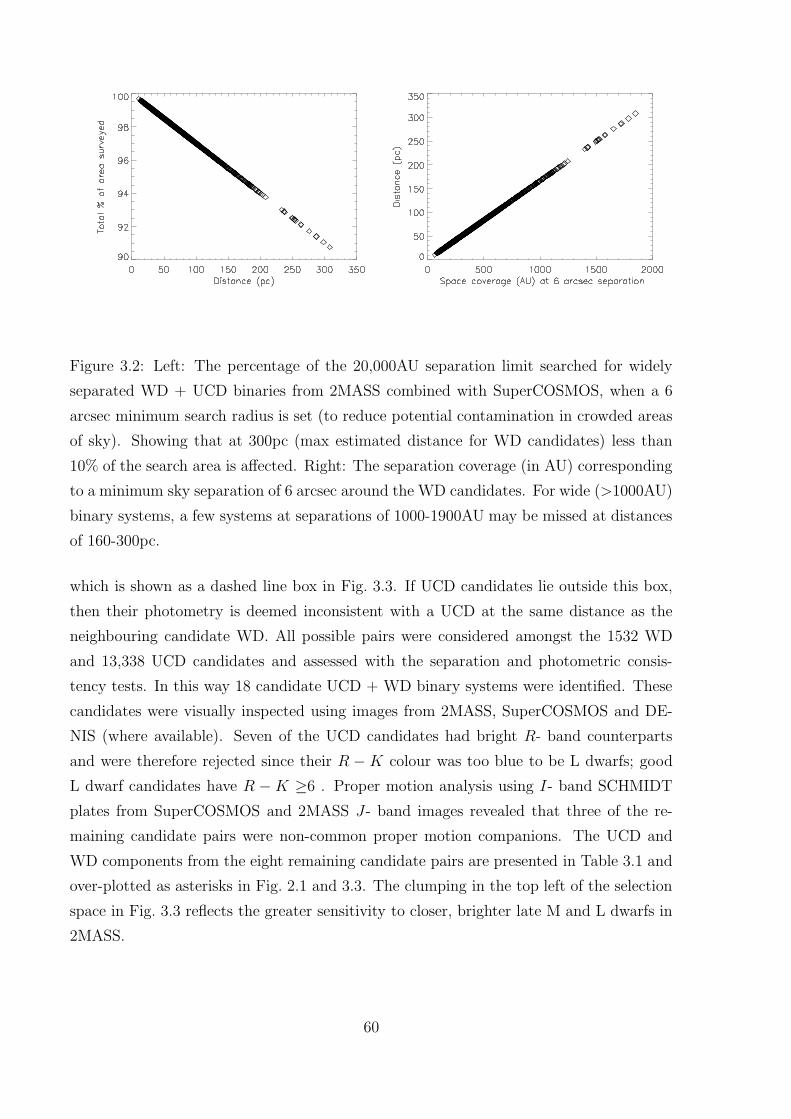
Figure 3.2: Left: The percentage of the 20,000AU separation limit searched for widely
separated WD + UCD binaries from 2MASS combined with SuperCOSMOS, when a 6
arcsec minimum search radius is set (to reduce potential contamination in crowded areas
of sky). Showing that at 300pc (max estimated distance for WD candidates) less than
10% of the search area is affected. Right: The separation coverage (in AU) corresponding
to a minimum sky separation of 6 arcsec around the WD candidates. For wide (>1000AU)
binary systems, a few systems at separations of 1000-1900AU may be missed at distances
of 160-300pc.
which is shown as a dashed line box in Fig. 3.3. If UCD candidates lie outside this box,
then their photometry is deemed inconsistent with a UCD at the same distance as the
neighbouring candidate WD. All possible pairs were considered amongst the 1532 WD
and 13,338 UCD candidates and assessed with the separation and photometric consis-
tency tests. In this way 18 candidate UCD + WD binary systems were identified. These
candidates were visually inspected using images from 2MASS, SuperCOSMOS and DE-
NIS (where available). Seven of the UCD candidates had bright R- band counterparts
and were therefore rejected since their R − K colour was too blue to be L dwarfs; good
L dwarf candidates have R − K ≥6 . Proper motion analysis using I- band SCHMIDT
plates from SuperCOSMOS and 2MASS J- band images revealed that three of the re-
maining candidate pairs were non-common proper motion companions. The UCD and
WD components from the eight remaining candidate pairs are presented in Table 3.1 and
over-plotted as asterisks in Fig. 2.1 and 3.3. The clumping in the top left of the selection
space in Fig. 3.3 reflects the greater sensitivity to closer, brighter late M and L dwarfs in
2MASS.
60

Table 3.1: Candidate UCD + WD binary systems. Coordinates are J2000. Photometry
is from 2MASS, SuperCOSMOS and DENIS (where available). The last three columns
show which UCD candidates have second epoch imaging (see §3.3), which pairs have
been confirmed (or not) through common proper motion and which candidates have been
confirmed as a UCD or WD with spectroscopy (see §3.3).
Name RA DEC B- R- I- J - H- K- Sep 2nd CPM Spec
(arcsec) epoch
UCDc-1 00 30 06.26 -37 39 48.2 - - 18.30 15.2 14.4 13.8 89 IRIS2 Y Y
WDc-1 00 30 11.90 -37 40 47.2 16.77 16.35 15.97 16.1 15.8 - Y
UCDc-2 00 56 14.71 -40 36 03.6 - - - 15.8 15.0 14.3 922 IRIS2 N -
WDc-2 00 57 18.72 -40 45 29.6 15.80 15.07 13.67 12.4 - - -
UCDc-3 03 02 07.70 -09 41 57.1 - - 17.66 15.8 15.0 14.5 136 IRIS2 N -
WDc-3 03 02 03.00 -09 43 54.9 17.63 17.35 17.34 - - - -
UCDc-4 05 20 35.40 -18 54 27.7 - - 17.64 15.9 15.1 14.7 145 IRIS2 N -
WDc-4 05 20 40.03 -18 56 37.9 18.34 16.40 17.92 - - - -
UCDc-5 10 12 35.59 -10 51 02.2 - - 18.13 15.3 14.6 14.1 465 IRIS2 ? -
WDc-5 10 12 43.89 -10 43 33.8 19.48 18.34 17.87 - - - -
UCDc-6 10 40 43.41 -16 48 20.5 - - - 15.9 15.2 14.8 124 IRIS2 ? -
WDc-6 10 40 39.17 -16 50 08.3 20.34 19.54 19.12 - - - -
UCDc-7 14 05 37.54 -05 51 53.6 - - 17.80 15.8 15.2 14.6 164 - - -
WDc-7 14 05 44.98 -05 49 51.9 16.66 16.80 16.87 - - - -
UCDc-8 23 21 21.55 -13 26 28.3 - - - 14.5 13.5 13.1 73 IRIS2 ? -
WDc-8 23 21 14.38 -13 27 36.8 19.23 18.42 18.00 - - - -
Notes - ? Indicates uncertainty due to a small measured motion and high
uncertainties associated with the proper motion measurements (see text).
61

Figure 3.3: An MJ against J − K colour-magnitude diagram showing the location of the
companion UCD candidates (asterisks) when they are assumed to be at the same distance
as their associated WD candidate. The UCD selection criteria is indicated with a dashed
line and UCDs with known parallax from dwarfarchives.org are plotted as plus signs.
UCD-1 is also circled (see §3.3).
3.2.1 Proper motions of candidate systems
Second epoch images of candidate UCDs were taken with the Infrared Imager and Spec-
trograph, IRIS2 on the Anglo Australian Telescope (AAT) during service observations on
2006 July 7 and 2006 December 8, with J-, H- and Ks- band filters. The images were
reduced using the standard oracdr package for IRIS2; this included de-biasing to remove
the CCD DC signal from the images, flatfielding to remove any pixel to pixel variations
and any imperfections in the optics (i.e. dust). The data were dark subtracted, removing
any thermal background inherent to the CCD and bad pixels were interpolated over to
prevent inaccurate flux measurements in the areas they occupy on the image. Finally
the jittered images (a 5 point jitter was used) were mosaiced together to create a final
reduced image.
The iraf routines geomap and geoxytran were used to create a transformation
of the X and Y position shift and scale between the available multi-epoch images, using
an average of 15 reference stars. Proper motions were calculated by multiplying the
motion (in pixels) by the pixel scale of IRIS2 (0.448 arcsec/pixel) and then dividing by
the baseline (in yrs), to give a relative proper motion in arcsec/yr. In addition a correction
was applied to the derived proper motions to account for the average (but small) proper
62

motion of the reference stars. Uncertainties were initially estimated from centroiding
accuracies (typically 0.5 pixels) combined with the residuals associated with the derived
transformations.
Amongst the eight candidate binary pairs, three of the UCD candidates were ruled
out since they are not common proper motion companions (at >3σ), three remain un-
certain due to the relatively small motion expected between epochs (compared to the
uncertainties associated with the inter-epoch transforms) and one remains unobserved
(see Table 3.1 for a summary of these results).
Second epoch IRIS2 measurements of candidate UCDc-1 (2MASS J0030 − 3739)
revealed a significant motion over the 6.8 yr baseline between the 2MASS first epoch and
the IRIS2 second epoch images. The large field of view of IRIS2 (7 x 7 arcmin) allowed the
proper motion of both the UCD and the WD candidate to be measured from the same
two-epoch image set, which clearly revealed the common proper motion. Final proper
motion measurements and uncertainties were based on four individual measurements:
pairing up J-, H- and K- band images from the 2MASS and IRIS2 epochs appropriately,
as well as pairing up a SuperCOSMOS I- band as first epoch with the IRIS2 J- band
image as second epoch. The last combination is over a relatively longer baseline of 15.86
yr, although this may suffer from larger chromatic effects due to the different bands.
The final proper motions were an average of these four measurements and the associated
uncertainties were estimated from their standard deviation. The measured proper motions
of the pair are given in Table 3.4. Multi-band BRIJHK 2 x 2 arcmin finder charts centred
on 2MASSJ0030 − 3739 are shown in Fig. 3.4.
3.3 A wide WD + UCD binary
3.3.1 Spectral classification of UCDc-1: 2MASSJ0030-3739
Spectroscopic observations of one candidate (UCD-1; see Table 3.1) were also obtained
with IRIS2 on the AAT on 2006 September 8. The long slit mode was used with a 1 arcsec
slit width in the J- long and H- short grisms, covering wavelength ranges 1.1 − 1.33µm
and 1.46 − 1.81µm with a dispersion of 0.225 nm/pixel and 0.341 nm/pixel, respectively
(R ∼ 2400). A total exposure time of 20 minutes in each band was obtained and the
target was nodded along the slit in an “ABBA” pattern with individual exposure times
of 300s. Standard dome flats and Xenon arcs were taken at the end of the night and an
63

Figure 3.4: SuperCOSMOS and 2MASS images show UCDc-1 (2MASSJ0030 − 3739;
squares) and WDc-1 (2MASSJ0030 − 3740; circles).
64
F5V star was observed at a similar airmass to the target to provide a telluric correction.
The observing conditions were reasonable with an average seeing of 0.8 − 1.2 arcsec.
Standard iraf routines were used to reduce the spectra including flat fielding. A
flatfield image was created from dome flat images by removing ′lamp on′ images from ′lamp
off′ images, then median combining them using the imarith routine. This flatfield image
was then normalised to ∼1 by creating a smoothed flatfield image, using the boxcar
routine to provide the average flux in a box 11 pixels on each side. This was then divided
out of the flatfield image to create a normalised masterflat. Each of the A and B images
of the object, standard star and arcs were divided by the masterflat image. Cosmic rays
and bad pixels were removed using an IDL program to identify bad pixels or groups
of bad pixels and replace them with an average value in a 10 pixel box surrounding
the bad pixel location. A-B pairs, containing a positive and negative object spectrum
were extracted with apall using a chebyshev function to fit the background and a third
order Legendre function (where points of deviation were removed) to trace the fit to the
spectrum. The wavelength calibration was done with a Xenon arc lamp spectrum, using
identify to reference the wavelength of the arc lines (from the line lists provided by the
AAO; www.aao.gov.au/iris2) and the dispcor routine was used to correct the dispersion
of the spectrum. This method was repeated for each of the differenced A-B pairs, and the
wavelength calibrated spectra were median combined and flux calibrated by dividing the
object spectrum by the telluric standard, then multiplying by the spectra of a blackbody,
created from the bbody routine in the starlink package figaro for a Teff= 6530K
(appropriate for a F5V star; see Allen’s astrophysical quantities). The annotated spectra
are shown in Fig. 3.5 and Fig. 3.6.
Spectral ratios
An estimate of the spectral type for 2MASSJ0030 − 3739 was based on spectral ratios
used in previously published work. The J- band spectral coverage is 1.1−1.35µm. In this
range the FeH ratio from Slesnick, Hillenbrand & Carpenter (2004) and the J- FeH and
H2OA ratio from McLean et al. (2003) were used. A ratio of 0.854 for FeH was measured,
where FeH is the ratio of the median flux at 1.20 and 1.23µm using a bandwidth of 0.01µm
(1.20/1.23µm; bandwidth=0.01µm). Using the spectral type relation from Slesnick, Hil-
lenbrand & Carpenter (2004), a spectral type of M9 was estimated from this ratio. The
J- FeH (1.20/1.185µm; bandwidth = 0.04µm) ratio of 0.85 combined with the spectral
type relations from fig. 12 of McLean et al. (2003) gives a spectral range M8-L3. At
65

Figure 3.5: J- band spectra of 2MASSJ0030 − 3739 (thin grey line), shown with com-
parison spectra (thick line) of an M7, M9 and L1 type (top to bottom) from Cushing et
al. (2005) overlaid. Also shown are the spectral ratios (J-FeH, FeH and H2OA) used for
spectral typing and the features (NaI, KI and AlI) are shown.
Figure 3.6: H- band spectra of 2MASSJ0030 − 3739 (thin grey line), shown with com-
parison spectra (thick line) of an M7, M9 and L1 type (top to bottom) from Cushing et
al. (2005) overlaid. Also shown are the spectral ratios (FeH, H2OB and H2OC) used for
spectral typing and the main KI feature.
66

the edge of the spectral coverage in the J- band, when strong water vapour absorption
starts to appear, is the H2OA ratio (1.343/1.313; bandwidth = 0.004µm). This ratio was
measured as 0.554. The relation between H2OA and spectral type in fig. 11 of McLean
et al. (2003) indicates an ∼L1 type from this ratio.
The H- band spectrum covers wavelengths 1.45− 1.81µm, for which the H2O ratios
from Reid et al. (2001a)[H2OC ] and McLean et al. (2003)[H2OB] were used. The H2OC
ratio at 1.788/1.722µm with a bandwidth of 0.004µm was measured as 0.697 and indicates
an L1.5±2 type. The H2OB ratio (1.48/1.60µm; bandwidth=0.02µm) of 0.9 is consistent
with an M8-M9 type. All of the spectral ratios considered are indicated by dotted lines
in Fig. 3.5 and Fig. 3.6 and the spectral ratio results are summarised in Table 3.2.
Comparison to template spectra
Template spectra of known late M and early L dwarfs were used to make a comparison
to the overall profile of 2MASSJ0030− 3739, as well as a comparison to the absorption in
spectral features such as the KI (1.168, 1.179 and 1.243, 1.254µm), NaI (1.138, 1.141µm),
AlI (1.311, 1.314µm) doublets in the J- band and the blended KI doublet (1.517µm) and
FeH (1.58, 1.59 and 1.62µm) in the H- band. In general alkali metal lines weaken at
the M/L boundary (McLean et al. 2000), but the NaI, AlI, FeH and KI doublets are
still clearly recognisable for the purposes of a comparison. The spectra of an M7(VB8),
M9(LHS2924) and L1(2MASSJ1439 + 1929) from Cushing, Rayner & Vacca (2005) were
rebinned to the dispersion of the NIR spectra and normalised at 1.26 and 1.64µm in the
J- and H- bands respectively (Fig. 3.5 and 3.6). Visual inspection of the blended line
features reveal the spectra are most consistent with an ∼M9 type.
Equivalent widths
Equivalent widths for the four neutral alkali (KI) lines present in the J- band spectra
were calculated using the methods of McLean et al. (2003). An IDL program was used to
interactively determine the equivalent width of each KI line, which were compared with
those of McLean et al. (2003) to estimate a spectral type from each line (see their table
7). In order to reduce the amount of bias when selecting the reference continuum, the
process was repeated 12 times using a continuum measured at different relative positions
(within 0.05 A from the centre of the line) and a mean of the measurements taken. A
67

Table 3.2: Estimated spectral types for 2MASSJ0030 − 3739.
Method Reference Spectral type
Ratio FeH (1.200/1.230µm) Slesnick (’04) M9′′ J- FeH (1.185/1.200µm) McLean (’03) M8-L3′′ H2OA (1.313/1.343µm) ′′ ∼L1′′ H2OC (1.722/1.788µm) Reid (’01) L1.5±2′′ H2OB (1.480/1.600µm) ′′ M8-M9
SC J- ... M9±1
SC H- ... M9±1
EW KI (@ 1.168µm) McLean (’03) M8-M9
EW KI (@ 1.177µm) ′′ M7-M8
EW KI (@ 1.243µm) ′′ M7-M8
EW KI (@ 1.254µm) ′′ M7-M8
Notes: SC- Spectral Comparison, EW- Equivalent Width.
width of 4.89 A at the 1.168µm line indicates an M8/9; while the other three KI line
widths at 1.177, 1.243 and 1.254µm are all consistent with an M7/8 type.
Analysis of the spectra of 2MASSJ0030 − 3739, through the use of spectral ratios,
comparison to template spectra and equivalent widths are summarised in Table 3.2, and
are consistent with a spectral type M9±1. The relation between spectral type and abso-
lute magnitude from Dahn et al. (2002) was used to calculate a range in MJ of 10.85−12.04
for the spectral range M8-L0. Thus, combining this with the measured J- band magnitude
from 2MASS, it is estimated that 2MASSJ0030 − 3739 is at a distance of 41 − 75 pc.
3.3.2 Spectral classification of WDc-1: 2MASSJ0030-3740
A spectrum of WDc-1 (2MASSJ0030 − 3740) was obtained with FORS1 on the VLT
on 2007 January 24, with Directors Discretionary Time in programme 278.C-5024(A),
using the longslit mode in the optical wavelength range 3800 − 5200A and a dispersion
of 50 A/mm. Three integrations of 600s were taken, giving a total exposure time of 30
minutes. Spectra of a DC WD and a standard F-type star were also taken and used for
calibration. Sky flats were taken and HgCd arcs were used for wavelength calibration.
68

Figure 3.7: Optical spectrum of the confirmed white dwarf WDc-1 (2MASSJ0030−3740),
flux calibrated and normalised at 4600A.
Standard IRAF packages were used to reduce the spectra including debiasing (by
creating a master bias frame from median combined images and subtracting this from the
object, standard star, flat field and arc images), flat fielding and removal of bad pixels.
The three spectra were then extracted and wavelength calibrated as described in §3.3.1.
The resulting spectra of both WDc-1 and the standard were divided by the featureless
DC WD spectrum, which has no intrinsic spectral features, enabling correction for the
instrumental response. The standard star was then used for flux calibration and the final
spectrum of 2MASSJ0030 − 3740 is shown in Fig. 3.7.
WD parameters, Teff and log g were derived from a fit of the Balmer lines using
the fitting routine fitprof described in Napiwotzki, Green & Saffer (1999). The WD
spectrum was modelled using an extensive grid of spectra computed with the model atmo-
sphere code of Detlev Koester described in Finley, Koester & Basri (1997). Observational
and theoretical Balmer line profiles were normalised to a linear continuum and the at-
mospheric parameters determined with a χ2 algorithm. The best fit is shown in Fig. 3.8.
The results are Teff = 7600 ± 20K and log g = 8.09±0.04 (formal uncertainties from the
fit routine to one sigma).
69

Table 3.3: Fit results and derived quantities for WD mass, cooling age and absolute
magnitude for the corrected and uncorrected case discussed in §3.3.2.
Teff log (g) M tcool MV
K dex M� Gyr
solution 1 7600 8.09 0.65 1.48 13.4
solution 2 7600 7.79 0.48 0.94 12.9
Realistic uncertainty estimates are often substantially larger than the formal statis-
tical estimates. Napiwotzki et al. (1999) derived a relative uncertainty of 2.3% in Teff and
0.075 dex in log g from a sample of DA WDs analysed using the same fitting method. This
temperature uncertainty was adopted for the following estimates, but the gravity determi-
nation is likely subject to a systematic overestimate. The mass distribution of WDs peaks
close to 0.6M� (e.g. Napiwotzki, Green & Saffer 1999; Bergeron, Gianninas & Boudreault
2007), corresponding to log g values close to 8.0. Spectroscopic investigations applying
the method have shown a trend of the log g distribution peaking at increasingly higher
values for decreasing temperatures (Bergeron, Gianninas & Boudreault 2007). This trend
starts at 11,500K putting the WD analysed here in the affected region. Taken at face
value, this would indicate on average higher masses for cool WDs. However, as argued by
Bergeron, Gianninas & Boudreault (2007) and Engelbrecht & Koester (2007) this can be
ruled out. A source of extra line broadening must be present in these stars. However, the
exact nature of this mechanism is still under discussion and as pointed out in Bergeron,
Gianninas & Boudreault (2007) anecdotal evidence suggests that some stars are affected
and others are not.
A pragmatic approach was taken here, where a large sample of DA white dwarfs were
used from observations taken in the course of the SPY programme (Napiwotzki et al. 2001)
to derive an empirical correction. Spectra of these stars have been previously analysed
using the same model grid and very similar analysis methods as for the WD discussed
here. The estimated shift in log g distribution caused by the unknown mechanisms is
0.3 dex in the Teff = 7500 − 8000K range. The corrected gravity is thus log g=7.79. As
mentioned above it is not entirely clear whether all cool WDs are affected. Thus the
corrected and uncorrected gravity values will be used for further discussion. WD masses
and cooling ages were calculated by interpolation in the Benvenuto & Althaus (1999)
cooling tracks for WDs with thick hydrogen envelopes. Results are listed in Table 3.3.
70

Figure 3.8: Model atmosphere fit to the Balmer lines of 2MASSJ0030 − 3740 giving best
fit parameters of Teff = 7600K and log g=7.79. Observed and theoretical fluxes were
normalised to the continuum. Line profiles are shifted for clarity.
71

3.3.3 A randomly aligned pair?
In order to determine if the new system is a bonafide UCD + WD binary, the likelihood
that two such objects could be a line-of-sight association with photometry and proper
motion consistent with binarity by random chance has been statistically assessed. To do
this, firstly the UCD luminosity function of Cruz et al. (2007) was taken, which gives
a number density of (4.9±0.6)×10−3 UCDs per pc3 for M7-M9.5 types. Then a volume
associated with 1532 circular areas on the sky (one for each of the WD candidate sample),
with radii of 89 arcsec (separation of the components) and a line-of-sight depth of 58±17pc
(approximate distance to the new M9 UCD, using relations from Dahn et al. 2002) were
calculated. This volume equates to 58±26 pc−3, giving a total expected number of 0.28
UCDs to be within 89 arcsec of one of the WD candidates.
To factor in the probability that two objects might have a common proper motion at
the same level as the measurements, a magnitude-limited sample (R <20) was downloaded
from the SuperCOSMOS Science Archive (SSA), applying the same minimum proper
motion requirement that was used to create the WD candidate sample. A magnitude
limited sample of 160 sources, selected from a large circular sky radius of 90 arcmin
centred on the WD. A proper motion vector-point-diagram was constructed and sources
counted that were found to be within the 2σ uncertainty circle of the measured UCD
proper motion. Four of the 160 sources had proper motion consistent with the UCD,
suggesting a probability of 2.4±1.2% that such common proper motion could occur by
random chance (where Poisson uncertainties associated with this and other samples were
considered here).
An additional requirement fulfilled by the UCD + WD system is that the colour-
magnitude information must be consistent with a common distance (see Fig. 3.3) and
53% (786 ± 28) of the WD candidate sample were found to be photometrically consistent
with being at the same distance as the UCD.
Finally considered was the fraction of WD candidates that might be spurious and
thus not able to contribute to non binary line-of-sight associations where the WD has been
confirmed spectroscopically. In the magnitude range R < 14, where MS99 is thought
to be essentially complete, it was find that 66% of our WD candidates are included
in the MS99 catalogue. This suggests that, at least for brighter magnitudes, the WD
candidates presented here are relatively free from contaminating objects, and that the
selection techniques are robust. While it cannot be guaranteed that the same low-level of
72

contamination applies to the full magnitude range, a conservative approach was taken, by
assuming that the full WD candidate sample could potentially contribute to non-binaries
that appear to be UCD + WD pairs.
Taking into account all these factors, it is estimated that one would expect 0.0036 ±
0.0025 randomly aligned UCD + WD pairs with ≤ 89 arcsec separation, proper motion
and photometry consistent with binarity at the level of the observations. The likelihood
of the system being merely a line-of-sight association is thus vanishingly small, and it can
thus be assumed that the UCD + WD pair is a gravitationally bound binary system.
3.3.4 Binary age
The age of the binary system can be constrained from the WD mass and cooling age.
For the corrected fit, 2MASSJ0030 − 3740 has a mass of 0.48M� and a cooling age of
0.94Gyr. The IFMR determinations of Weidemann (2000), Dobbie et al. (2004), Dobbie
et al. (2006), Ferrario et al. (2005), Catalan et al. (2008) and Kalirai et al. (2008) were
assessed to estimate a likely, initial-mass constraint for the main-sequence progenitor star
of 1 − 2M�. The main-sequence lifetime of a progenitor of this mass is likely >1Gyr
(probably several Gyr) and thus is not useful when trying to constrain the upper age
limit of the system. Note that if the WD mass were higher, for example if the helium
enrichment of the atmosphere is lower than typical (see §3.3.2) then the WD’s log g could
be as high as 8.1 dex, with a WD mass of ∼0.65M� and cooling age of ∼1.5Gyr. This
would allow the progenitor mass to be constrained to a likely range of > 2.7M�, giving
a main-sequence progenitor lifetime of < 0.83Gyr (Monteiro et al. 2006) and a binary
age constraint of 1.5 − 2.3Gyr. This possibility is instructive at least in demonstrating
the level of age constraints (with accompanying UCD constraints) that may be placed on
benchmark binaries of this type. However, it is not possible to judge the helium content
of the WDs atmosphere (if any) and thus only a lower limit can be confidently placed
on the age of this binary from the best fit cooling age for the WD, combined with an
estimate of the main-sequence lifetime of the progenitor, which is likely equal to or larger
than the WD cooling age. The age of the binary is thus > 1.94Gyr.
73

3.3.5 UCD properties
Teff , mass and log g have been estimated from the Lyon group DUSTY models (Chabrier
et al. 2000c; Baraffe et al. 2002), using the minimum age of the system (1.94Gyr) and
an estimated MJ for 2MASSJ0030−3739. The models indicate that 2MASSJ0030−3739
has Teff = 2000 − 2400K, mass=0.07 − 0.08M� and log g=5.30 − 5.35, placing it close
to the limit for hydrogen burning. Note that the estimated Teff is consistent with the
semi-empirical estimates of Golimowski et al. (2004) for an M9±1 dwarf, which use well
measured luminosities and a model constraint on radius (which changes by <10% for ages
of 1− 5Gyr) to determine Teff values spanning a wide range of spectral type. The full list
of properties for the binary are listed in Table 3.4.
3.4 Searching SDSS and UKIDSS
A search for widely separated binary systems from a selected sample of WDs and UCDs
from SDSS and UKIDSS (as described in §2.1.2 and 2.2.2) was conducted using a similar
method as was used for the 2MASS and SuperCOSMOS search (described in in §3.2).
3.4.1 Simulated numbers of WD + UCD binaries
The number of potential WD + UCD binary systems that could be detected in the full
coverage of SDSS and UKIDSS was estimated by Pinfield et al. (2006), who suggest that
50+13−10 benchmark systems (with ages known to 10%) could be found out to a limiting
magnitude of J≥19.0. The number of non-benchmark systems (where the WD <0.7M�)
that could also be identified is estimated at five times that number, suggesting that
up to 300 WD + UCD systems could be identified by combining UKIDSS with SDSS.
Corresponding photometric properties were also derived and are shown in Fig. 3.9. The
level of contamination from other objects such as high velocity stars (e.g. halo objects or
red giants) was estimated at ∼400, which is comparable to the number of real systems
expected via photometric selection alone. However, measuring a common proper motion
for the components of potential systems should remove the majority of the contamination.
74

Table 3.4: Parameters of the binary 2MASSJ0030− 3739 + 2MASSJ0030− 3740 and its
components.Parameter Value
Separation on sky ............ 89 arcsec
Estimated distance ............ 41 − 59 pc
Estimated line-of-sight
separation ............ 3650 − 5250 AU
Minimum age of system ............ > 1.94 Gyr
Ultracool Dwarf
RA ............ 00 30 06.26
DEC ............ -37 39 48.2
2MASS designation ............ 2MASSJ0030 − 3739
Distance ............ 41 – 75pc
2MASS J ............ 15.2± 0.05
2MASS H ............ 14.4± 0.05
2MASS Ks ............ 13.8± 0.06
DENIS I ............ 18.4± 0.23
DENIS J ............ 15.06± 0.14
SuperCOSMOS I ............ ∼18.3
µ RA ............ -130±30 mas yr−1
µ DEC ............ -70±20 mas yr−1
Spectral Type ............ M9±1
Mass ............ 0.07 − 0.08 M�
Teff ............ 2000 − 2400 K
log g ............ 5.30 − 5.35 dex
White Dwarf
RA ............ 00 30 11.9
DEC ............ -37 40 47.2
2MASS designation ............ 2MASSJ0030 − 3740
Distance ............ 27 − 59 pc
2MASS J ............ 16.1± 0.11
2MASS H ............ 15.8± 0.15
DENIS I ............ 16.2± 0.07
DENIS J ............ 15.9± 0.22
SuperCOSMOS B ............ ∼16.77
SuperCOSMOS R ............ ∼16.35
SuperCOSMOS I ............ ∼15.97
µ RA ............ -83±30 mas yr−1
µ DEC ............ -70±12 mas yr−1
Spectral Type ............ DA
Teff ............ 7600±175 K
log g ............ 7.79 − 8.09 dex
Mass ............ 0.48 − 0.65 M�
WD cooling age ............ 0.94 − 1.5 Gyr
WD progenitor age ........... > 1 Gyr
75

Figure 3.9: Simulated WD + UCD J- against g- magnitude diagram from Pinfield et
al. (2006), showing a simulated population of WD + UCD binaries (dots) covering 10%
of the sky for J≥16.0. Potential benchmark systems (WD ≥0.7M�) are shown as plus
symbols.
3.4.2 Binary selection
To select binary system candidates, firstly distance constraints were placed on the sample
of WD candidates selected from SDSS using a CMD for WDs with known parallax from
McCook & Sion (1999) in the SDSS colour system as shown in Fig. 3.10. In the same way
as described in §3.2, this was used to estimate a lower distance for the WD candidate and
thus a maximum separation based on a mass of 1.2M�. UCD candidates were searched
for out to an angular separation from each WD candidate corresponding to a projected
separation of 20,000AU at this estimated distance. In order for a good UCD companion
to be selected it must have a distance consistent with the WD it is paired with. This
was assessed by placing the candidate UCD companion on a MJ against J − H CMD,
where MJ was calculated from the WD lower distance estimate and the UKIDSS J- band
magnitude. The J − H colour was chosen here, instead of the previously used J − K
colour (for L dwarf candidates in 2MASS), as T dwarfs have bluer NIR colour and can
thus be very faint in the K- band. Selection regions were defined using known L and T
dwarfs with measured parallax from dwarfarchives.org. The regions defining these
areas are shown as dotted (L) and dashed (T) line boxes, as illustrated in Fig. 3.11 and
76

Figure 3.10: A WD colour-magnitude diagram for MS99 WDs with known parallax
(crosses with error bars). Photometry is on the SDSS system. Overplotted are model
cooling tracks (see §3.4.1) for WD masses of 0.5, 0.7 and 1.2M� (dotted, dashed and
dot-dashed lines respectively). The selected WD region in the CMD lies between the two
solid lines.
were chosen to select objects with the most compelling UCD colours whilst minimising
contamination from main-sequence stars. It is also noted that there is some cross over in
the position of some late L and early T dwarfs, as is also shown by Knapp et al. (2004).
The selection used here is flexible enough to account for this by allowing objects that have
L dwarf Y − J and J − H colours, that also pass the T dwarf MJ , J − H CMD criteria
to be selected as possible L/T transition objects.
Candidate early/mid L dwarfs were selected if they occupy the L box in two-colour
space (Fig. 2.5) and the corresponding L box in colour-magnitude space (Fig. 3.11). If an
object is found in the L box in two-colour space and the T box in colour-magnitude space
then is it selected as an L/T transition object, likewise a candidate T dwarf is selected if
its position lies in the T box in both colour and colour-magnitude selections. The criteria
for the three selections are outlined here:
77

Figure 3.11: A UCD colour-magnitude diagram for L (plus symbols) and T (diamonds)
dwarfs with known parallax from dwarfarchives.org. The selection regions for L and
T dwarfs are overplotted as dotted and dashed lines, respectively.
Early/Mid L dwarf colour and magnitude selection criteria:
0.4 < J − H < 1.2, 0.9 < Y − J < 1.5
and
11.0 < MJ < 15.0, MJ < 8.5(J − H) + 7.0
Late L/Early T dwarf (i.e. L/T transition objects) colour and magnitude selection
criteria:
0.4 < J − H < 1.2, 0.9 < Y − J < 1.5
and
13.5 < MJ < 17.0, MJ > 8.5(J − H) + 7.0
Mid/Late T dwarf colour and magnitude selection criteria:
−0.5 < J − H < 0.4, 0.9 < Y − J < 1.25
and
13.5 < MJ < 17.0, MJ > 8.5(J − H) + 7.0
78

An IDL program was written to search for candidate pairs amongst the 22,087 WD
and 24,293 UCD candidate objects using these selection criteria, which resulted in a
sample of 517 candidate binary systems.
3.4.3 Candidate WD + UCD systems
As SDSS covers a large section of sky common to that of UKIDSS, the UCD candidates
were cross matched with objects in the SDSS DR6 database, using the cross matching
facility in a 2 arcsec radial search, which should detect any optical component for objects
with a proper motion of less than ∼1 arcsec/yr. The UCD candidate sample was then
split up into two categories; optical and non-optical detections. Properly assessing the
optical non detections would require further follow-up beyond the scope of this thesis.
For the optical detections additional colour cuts were used, based on the objects optical
and optical-NIR colours.
Hawley et al. (2002) show that L and T dwarfs are separated quite well using i − z
and z − J colours and suggest that i − z > 1.6 would select M8 and later type dwarfs.
Indeed Fan et al. (2001) and Chiu et al. (2006) select L and T dwarfs where i − z > 2.2
and z − J > 2.0. An i − r colour could also be used, however many UCDs are very faint
in the r- band and photometry can be unreliable. Following this approach, good L and
T dwarf candidates were selected if they had i and z band SDSS counterparts with ≥5σ
detections (corresponding to the approximate SDSS 5σ limits; i < 21.3 and z < 20.8),
i−z > 1.75, and z−J > 2.0. Additionally a subset with 1.6 < i−z < 1.75 and z−J > 2.0
were also selected as candidate UCDs. Non i− band detections or ′drop outs′ were also
considered, where the z − J colour limits are consistent with being UCD like.
By including this optical selection the candidate list was reduced from 517 to 156.
68 have no optical counterpart within 2 arcsec of their NIR coordinates (implying i > 21.3
and z > 20.8) and are shown in Tables 3.11 and 3.12 as candidates named nBINx (where x
is the identifying number). 18 are i− band drop outs and are shown in Tables. 3.9 and 3.10
as candidates with name iBINx. 34 are good late M candidates, having 1.6 < i− z < 1.75
and z − J > 2.0 (Shown as candidates mBINx in Tables. 3.7 and 3.8). 36 are good L and
T candidates based on their optical and optical-NIR colours (i−z > 1.75 and z−J > 2.0)
and labelled as candidates bBINx in Tables. 3.5 and 3.6. These 156 candidates were also
eyeballed in the UKIDSS/WFCAM images and the SDSS optical images to remove any
spurious survey detection or non-star like objects. None of the candidates showed any
79
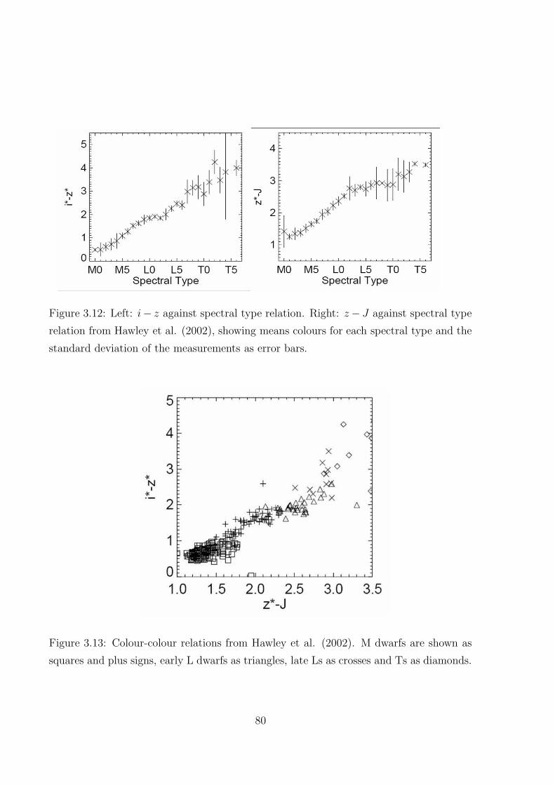
Figure 3.12: Left: i− z against spectral type relation. Right: z − J against spectral type
relation from Hawley et al. (2002), showing means colours for each spectral type and the
standard deviation of the measurements as error bars.
Figure 3.13: Colour-colour relations from Hawley et al. (2002). M dwarfs are shown as
squares and plus signs, early L dwarfs as triangles, late Ls as crosses and Ts as diamonds.
80

sign of being spurious and are thus plotted in Figs. 3.14 and 3.15.
In addition the WD candidates were cross matched with the SDSS spectroscopic
catalogue to check if any had spectra that could confirm them, or not as such. Of the
156 candidate WDs, 71 had spectra available from SDSS. Of these 36 are flagged as being
WD (DA) targets and 35 are flagged as being ′star′ like. This classification may not just
contain main-sequence stars or late-type stars, but may include more unusual WD types
(DB, DC, DO, DQ, DZ) as well as unresolved, spectroscopic binaries containing a WD
member. Proper motion measurements were also checked for in the SDSS archive, which
are measured by matching SDSS positions against the USNO-B1.0 catalogue (Monet et al.
2003). Details of all 156 candidate binary pairs are shown in Tables. 3.6 - 3.12.
3.4.4 Second epoch imaging and proper motion analysis of can-
didate UCDs
One of the candidate binary systems (bBIN1) has spectroscopically confirmed components
as a DA WD and an L3 dwarf, however on inspection of the published proper motion of
the WD (from SDSS) and the L dwarf (Jameson et al. 2008) they do not appear to share
a common proper motion and this pair were thus ruled out as a potential binary system.
Additional pairs were prioritised from the list of candidates (where the WD compo-
nent had a measured proper motion of >100mas/yr) for follow-up second epoch imaging
on IRIS2/AAT during 2008 20-24 February. Nine candidates were imaged in the J-, H-
and K- bands during poor weather time (seeing > 2 arcsec). The images were reduced us-
ing the oracdr package for IRIS2 and proper motions calculated using the iraf routines
geomap and geoxytran using an average of 15 reference stars, as is described in §3.3.1.
In the majority of cases the motion was less than a pixel and the baseline on average only
∼1 yr. Combined with high residuals of the transformations from the WFCAM/UKIDSS
images onto the IRIS2/AAT images resulted in high uncertainties in the measurements.
The proper motions of the nine UCD candidates, along with the measured proper motion
of the WD counterpart are shown in Table. 3.13. Uncertainties were calculated from the
residuals of the transformation combined with centroiding uncertainties of ±0.5 pixels.
Of the nine candidates measured two were deemed to be non-common proper motion and
seven remain uncertain. In order to confirm the binary nature of these remaining seven
candidate systems an additional epoch image is needed, ideally with a longer baseline.
Candidates bBIN17, bBIN26 and bBIN29 appear to have a sizeable proper motion,
81

Figure 3.14: Left: A Y − J against J − H two-colour diagram. Right: An MJ against
J −H CMD of UCD candidate components of potential wide WD + UCD binaries. Blue
plus symbols show L and T dwarf candidates with good optical colours, red asterisks
are i− band drop outs, red diamonds are non-optical detections and black triangles are
UCD candidates with good optical colours, also overplotted are main-sequence stars as
green dots. The open square shows the widely separated UCD candidate system from the
spectroscopic WD + M dwarf (nBIN7; see §3.4.4). Also shown are the L and T dwarf
selection regions (dotted and dashed boxes, respectively).
82

Figure 3.15: A u−g against g−r two colour diagram showing WD candidate components
of potential wide WD + UCD binaries. Blue plus symbols show WD candidates whose
L and T dwarf candidate counterparts have good quality optical colours, red asterisks
are i− band drop outs and red diamonds are optical non-detections, also overplotted are
spectroscopically confirmed WDs as green crosses. The open square shows the widely
separated WD candidate that appears to be an unresolved WD + M dwarf binary system
(nBIN7; see §3.4.4).
83
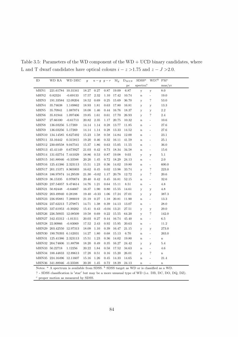
Table 3.5: Parameters of the WD component of the WD + UCD binary candidates, where
L and T dwarf candidates have optical colours i − z >1.75 and z − J >2.0.
ID WD RA WD DEC g u − g g − r Mg DMIN SDSSa WD?b PMc
pc spectra? mas/yr
bBIN1 221.61784 10.31341 18.27 0.27 0.87 19.09 6.87 y y 8.0
bBIN2 0.82324 -0.69133 17.57 2.32 1.10 17.42 10.74 n - 19.0
bBIN3 191.33584 12.09204 18.52 0.69 0.25 15.69 36.70 y ? 53.0
bBIN4 35.74638 1.149862 18.93 1.81 0.63 17.80 16.81 y y 13.3
bBIN5 35.70941 1.087874 18.08 1.46 0.44 16.76 18.37 y y 2.2
bBIN6 35.81944 1.097406 19.85 1.61 0.61 17.70 26.93 y ? 2.4
bBIN7 27.66100 -0.61713 20.82 2.35 1.17 20.75 10.32 n - 10.6
bBIN8 136.03256 5.17269 14.14 1.14 0.28 13.77 11.85 n - 27.6
bBIN9 136.03256 5.17269 14.14 1.14 0.28 13.33 14.52 n - 27.6
bBIN10 134.14585 6.627492 15.23 1.58 0.58 14.84 12.00 n - 23.1
bBIN11 33.16442 0.315815 19.20 0.46 0.32 16.11 41.59 n - 25.1
bBIN12 230.69558 9.047541 15.37 1.86 0.63 15.05 11.55 n - 36.0
bBIN13 45.41149 0.673927 21.03 0.42 0.73 18.34 34.58 n - 15.6
bBIN14 131.02754 7.441029 18.86 0.53 0.87 19.08 9.03 y y 5.1
bBIN15 341.88946 -0.33588 20.20 1.45 0.72 18.29 24.13 n - 2.0
bBIN16 125.41386 2.323113 15.51 1.23 0.36 14.02 19.80 n - 600.0
bBIN17 201.15371 8.965003 16.62 0.45 0.02 13.98 33.74 y ? 223.0
bBIN18 186.97874 14.29539 21.30 -0.02 1.17 20.78 12.72 y ? 20.6
bBIN19 36.15335 0.970674 20.40 0.42 0.45 16.81 52.15 n - 32.6
bBIN20 237.54057 9.474614 14.76 1.21 0.64 15.11 8.51 n - 4.8
bBIN21 50.82448 -0.64667 16.37 1.90 0.80 15.55 14.61 y y 4.8
bBIN22 203.49940 0.28188 19.40 -0.33 1.06 17.24 27.01 y y 387.3
bBIN23 226.95881 7.289019 21.19 0.27 1.18 20.81 11.90 n - 13.3
bBIN24 227.62213 7.279871 14.71 1.38 0.39 14.13 13.07 n - 28.0
bBIN25 337.61953 -0.39202 15.41 0.43 -0.04 13.21 27.51 y y 29.0
bBIN26 226.50935 12.08509 19.58 0.69 0.22 15.55 64.20 y ? 142.0
bBIN27 342.45312 -1.01311 20.03 0.27 0.44 16.74 45.40 n - 6.5
bBIN28 22.00966 -0.83069 17.52 2.43 0.92 15.95 20.63 n - 11.2
bBIN29 203.42550 12.97313 18.09 1.10 0.39 16.47 21.15 y y 273.0
bBIN30 190.70393 6.142031 14.27 1.80 0.68 15.13 6.70 n - 263.0
bBIN31 125.41386 2.323113 15.51 1.23 0.36 14.02 19.80 n - n
bBIN32 204.74606 11.88798 18.20 0.49 0.35 16.27 24.42 y y 5.4
bBIN33 50.22718 1.12256 20.22 1.84 0.58 17.52 34.63 n - 4.6
bBIN34 188.44833 12.89613 17.28 0.51 0.16 15.20 26.01 y ? n
bBIN35 224.16496 12.11607 15.16 1.26 0.45 14.33 14.65 n - 21.4
bBIN36 341.88946 -0.33588 20.20 1.45 0.72 18.29 24.13 n - n
Notes: a A spectrum is available from SDSS. b SDSS target as WD or is classified as a WD.
? - SDSS classification is ′star′ but may be a more unusual type of WD (i.e. DB, DC, DO, DQ, DZ).c proper motion as measured by SDSS.
84

Table 3.6: Parameters of the UCD component of the WD + UCD binary candidates,
where L and T dwarf candidates have optical colours i − z >1.75 and z − J >2.0.
ID UCD RA UCD DEC J J − H Y − J MJ Separation Separation i − z z − J
degs degs arcsec AU
bBIN1 222.10729 10.53281 14.42 0.90 1.38 15.23 1930.96 13270.12 2.089 2.861
bBIN2 0.89488 -0.21635 16.70 0.81 1.20 16.54 1729.25 18575.69 1.774 2.655
bBIN3 191.31236 12.07832 16.06 0.74 1.07 13.23 97.89 3593.47 1.855 2.606
bBIN4 35.95639 1.06426 17.15 0.62 1.12 16.02 816.43 13725.35 1.883 2.596
bBIN5 35.95639 1.06426 17.15 0.62 1.12 15.83 893.17 16415.80 1.883 2.596
bBIN6 35.95639 1.06426 17.15 0.62 1.12 15.00 507.24 13660.48 1.883 2.596
bBIN7 27.92090 -0.86569 15.02 0.73 1.21 14.95 1294.66 13366.27 2.081 2.591
bBIN8 135.75381 5.27047 15.90 0.70 1.15 15.53 1063.43 12602.39 1.876 2.540
bBIN9 135.75381 5.27047 15.90 0.70 1.15 15.09 1063.43 15446.30 1.876 2.540
bBIN10 134.58187 6.72768 17.32 0.74 1.18 16.92 1610.58 19333.80 1.890 2.518
bBIN11 33.21045 0.40327 16.64 0.60 1.03 13.55 355.81 14801.71 1.974 2.493
bBIN12 230.63575 9.12049 17.02 0.59 1.06 16.71 339.64 3926.21 1.916 2.455
bBIN13 45.47679 0.53108 17.60 0.70 1.12 14.90 565.40 19554.30 1.922 2.451
bBIN14 130.62033 7.77405 16.62 0.67 0.98 16.84 1893.79 17107.54 1.810 2.440
bBIN15 341.70443 -0.43699 17.32 0.61 1.11 15.40 759.06 18323.32 1.822 2.419
bBIN16 125.40509 2.21258 17.27 0.57 1.07 15.79 399.16 7905.84 1.824 2.410
bBIN17 201.17509 9.03326 17.03 0.60 1.02 14.39 257.50 8689.43 2.025 2.361
bBIN18 187.17242 14.44828 16.99 0.70 0.94 16.47 888.31 11304.07 1.792 2.332
bBIN19 36.17794 1.00201 17.60 0.64 1.12 14.01 143.38 7478.02 2.034 2.299
bBIN20 237.48178 9.05534 15.16 0.66 0.95 15.51 1524.16 12971.55 1.818 2.295
bBIN21 50.68592 -0.69307 17.74 0.59 1.00 16.92 526.05 7686.51 1.859 2.274
bBIN22 203.32255 0.21910 16.83 0.59 0.97 14.67 675.58 18253.91 1.766 2.261
bBIN23 227.37811 7.47357 15.34 0.52 0.90 14.96 1649.21 19640.76 1.785 2.254
bBIN24 227.37811 7.47357 15.34 0.52 0.90 14.76 1121.59 14663.43 1.785 2.254
bBIN25 337.66729 -0.52167 16.47 0.61 0.95 14.27 497.39 13683.39 1.802 2.253
bBIN26 226.49679 12.13369 17.76 0.57 1.02 13.72 180.70 11601.16 2.291 2.243
bBIN27 342.53976 -1.05936 17.51 0.57 0.96 14.23 353.56 16052.41 1.889 2.238
bBIN28 21.93350 -0.81522 18.04 0.67 1.05 16.46 279.77 5771.85 1.919 2.233
bBIN29 203.17382 13.03917 18.01 0.62 0.90 16.38 936.72 19814.91 1.831 2.229
bBIN30 190.22282 6.04823 15.97 0.61 0.95 16.84 1764.60 11836.43 1.752 2.226
bBIN31 125.44366 2.49658 17.25 0.72 0.91 15.77 633.63 12549.84 1.779 2.221
bBIN32 204.64443 11.92594 17.86 0.63 1.00 15.92 390.54 9540.46 1.858 2.218
bBIN33 50.31347 1.22600 18.03 0.61 0.93 15.33 484.93 16793.86 1.864 2.217
bBIN34 188.37532 12.89610 16.90 0.55 0.98 14.82 262.84 6838.23 1.922 2.207
bBIN35 224.19619 11.89695 16.37 0.62 0.90 15.54 796.80 11679.44 1.817 2.205
bBIN36 342.01263 -0.35698 18.08 0.59 1.13 16.16 449.86 10859.40 2.011 2.201
85

Table 3.7: Parameters of the WD component of the WD + late M dwarf binary candidates
selected from SDSS and UKIDSS.
ID WD RA WD DEC g u − g g − r Mg DMIN SDSSa WD?b PMc
pc spectra? mas/yr
mBIN1 194.49234 15.58729 20.17 0.47 1.15 20.67 7.96 y y 2.7
mBIN2 37.526710 1.15889 18.68 2.45 1.10 17.42 17.89 y ? 9.0
mBIN3 130.48223 2.39738 18.98 0.56 0.18 15.33 53.71 y ? 76.0
mBIN4 171.00970 0.07283 19.21 0.84 0.41 16.56 33.93 y y 1.7
mBIN5 170.94816 0.07170 16.45 1.05 0.45 16.79 8.53 y y 6.8
mBIN6 170.90776 0.04772 19.97 2.08 1.00 16.22 56.05 y ? 4.7
mBIN7 171.02877 0.04855 14.81 1.06 0.46 14.36 12.26 y y 1.1
mBIN8 170.92109 0.16004 16.97 1.69 0.73 15.29 21.71 y y 16.0
mBIN9 170.86575 0.20482 16.91 1.75 0.73 15.29 21.09 y y 1.1
mBIN10 170.94816 0.07170 16.45 1.05 0.45 14.34 26.43 y y 6.8
mBIN11 22.95191 0.70853 20.13 2.42 0.92 19.40 13.96 n - 19.9
mBIN12 22.97954 0.80239 16.10 2.06 0.94 16.00 10.48 n - 12.3
mBIN13 22.52972 0.44318 18.71 0.59 0.99 16.86 23.43 n - n
mBIN14 132.22509 7.42600 20.50 0.42 0.67 17.98 31.95 y ? 11.6
mBIN15 21.12783 0.96516 14.30 1.43 0.49 14.47 9.21 n - 22.6
mBIN16 209.07867 12.82209 19.40 0.58 0.21 15.46 61.47 y y 63.0
mBIN17 128.19085 8.57491 19.75 0.27 0.91 19.34 12.03 y y 4.0
mBIN18 128.15777 8.65947 15.26 1.40 0.55 14.67 13.12 n - 24.0
mBIN19 6.95838 -0.17319 18.19 0.17 0.28 15.85 29.48 n - 24.0
mBIN20 134.14585 6.62749 15.23 1.58 0.58 14.84 12.00 n - 23.0
mBIN21 229.01525 9.07295 17.26 0.51 1.04 17.14 10.52 y y 1.4
mBIN22 226.95881 7.28901 21.19 0.27 1.18 20.81 11.90 n - 13.3
mBIN23 173.14897 0.51127 19.26 1.34 0.63 17.79 19.66 y ? 0.6
mBIN24 173.17076 0.48829 18.60 1.40 0.63 17.78 14.57 y y 1.9
mBIN25 28.39781 0.26082 15.42 1.39 0.51 14.54 15.00 n - 20.9
mBIN26 358.90307 0.19146 17.22 1.25 0.24 15.63 20.75 n - 20.2
mBIN27 144.65409 7.24863 18.32 -0.04 0.53 17.23 16.47 n - 27.0
mBIN28 52.55113 -0.54926 20.87 -0.12 0.44 16.72 67.40 n - n
mBIN29 144.65409 7.24863 18.32 -0.04 0.53 17.23 16.47 n - 27.0
mBIN30 150.78918 7.63968 20.02 0.35 0.56 17.38 33.71 n - 5.7
mBIN31 125.41386 2.32311 15.51 1.23 0.36 14.02 19.80 n - 600.0
mBIN32 154.50003 8.63896 16.45 0.36 0.04 14.57 23.78 y y 235.0
mBIN33 203.42550 12.97313 18.09 1.10 0.39 16.47 21.15 y y 273.0
mBIN34 336.27880 0.14624 20.89 0.51 0.52 17.18 55.37 n - 5.0
Notes: a A spectrum is available from SDSS. b SDSS target as WD or is classified as a WD.
? - SDSS classification is ′star′ but may be a more unusual type of WD (i.e. DB, DC, DO, DQ, DZ).c proper motion as measured by SDSS.
86

Table 3.8: Parameters of the UCD component of the WD + late M dwarf binary candi-
dates selected from SDSS and UKIDSS.
ID UCD RA UCD DEC J J − H Y − J MJ Separation Separation i − z z − J
degs degs arcsec AU
mBIN1 194.19093 15.24543 16.04 0.60 1.00 16.53 1640.71 13068.13 1.68 2.50
mBIN2 37.58208 0.94662 17.21 0.61 1.03 15.94 789.73 14131.52 1.63 2.49
mBIN3 130.56904 2.40514 17.94 0.79 1.09 14.29 313.75 16851.89 1.62 2.46
mBIN4 170.93093 0.02568 16.27 0.71 1.00 13.61 330.49 11215.10 1.66 2.45
mBIN5 170.93093 0.02568 16.27 0.71 1.00 16.61 176.91 1510.71 1.66 2.45
mBIN6 170.93093 0.02568 16.27 0.71 1.00 12.52 115.14 6454.82 1.66 2.45
mBIN7 170.93093 0.02568 16.27 0.71 1.00 15.82 361.72 4436.00 1.66 2.45
mBIN8 170.93093 0.02568 16.27 0.71 1.00 14.58 485.00 10531.28 1.66 2.45
mBIN9 170.93093 0.02568 16.27 0.71 1.00 14.64 686.27 14480.38 1.66 2.45
mBIN10 170.93093 0.02568 16.27 0.71 1.00 14.15 176.91 4676.85 1.66 2.45
mBIN11 22.75033 0.43376 16.78 0.63 0.99 16.06 1226.81 17130.81 1.68 2.43
mBIN12 22.75033 0.43376 16.78 0.63 0.99 16.68 1562.67 16378.20 1.68 2.43
mBIN13 22.75033 0.43376 16.78 0.63 0.99 14.93 794.91 18626.26 1.68 2.43
mBIN14 132.24311 7.45873 17.99 0.69 1.25 15.47 134.52 4298.55 1.63 2.43
mBIN15 20.61140 0.97410 16.13 0.60 0.91 16.30 1859.43 17143.30 1.61 2.40
mBIN16 209.11651 12.85143 17.62 0.62 0.92 13.67 172.37 10597.37 1.69 2.36
mBIN17 127.82177 8.69213 17.16 0.59 0.96 16.76 1394.08 16784.49 1.70 2.36
mBIN18 127.82177 8.69213 17.16 0.59 0.96 16.57 1215.29 15946.19 1.70 2.36
mBIN19 7.02843 -0.26478 17.11 0.58 0.94 14.76 415.08 12237.70 1.61 2.32
mBIN20 134.17875 6.92316 17.30 0.74 1.02 16.90 1070.99 12856.52 1.63 2.32
mBIN21 229.18598 9.09350 16.85 0.66 0.93 16.74 619.06 6516.30 1.68 2.31
mBIN22 227.37811 7.47357 15.34 0.52 0.90 14.96 1649.21 19640.76 1.78 2.25
mBIN23 173.03959 0.36443 17.69 0.43 1.00 16.22 659.13 12962.98 1.66 2.25
mBIN24 173.03959 0.36443 17.69 0.43 1.00 16.87 649.44 9467.64 1.66 2.25
mBIN25 28.34825 0.29048 17.29 0.64 0.90 16.41 207.95 3119.87 1.61 2.23
mBIN26 359.05133 0.24332 17.57 0.58 0.97 15.98 565.43 11735.12 1.81 2.13
mBIN27 144.64984 7.54040 16.95 0.71 0.90 15.87 1050.45 17311.34 1.74 2.12
mBIN28 52.57260 -0.52133 18.03 0.59 0.90 13.88 126.83 8549.54 1.80 2.11
mBIN29 144.53628 7.37010 17.62 0.61 0.92 16.54 609.18 10039.17 1.73 2.07
mBIN30 150.78230 7.53372 18.04 0.46 0.92 15.40 382.26 12888.46 1.74 2.07
mBIN31 125.39768 2.05674 17.18 0.68 0.96 15.69 960.72 19028.31 1.71 2.06
mBIN32 154.51393 8.44871 17.41 0.62 0.91 15.53 686.72 16332.18 1.73 2.06
mBIN33 203.66122 12.86231 18.20 0.48 1.08 16.57 937.68 19835.23 1.95 2.05
mBIN34 336.23196 0.20562 17.84 0.61 0.98 14.13 272.27 15076.59 2.13 2.00
87

Table 3.9: Parameters of the WD component of the WD + UCD i- band drop out binary
candidates selected from SDSS and UKIDSS.
ID WD RA WD DEC g u − g g − r Mg DMIN SDSSa WD?b PMc
pc spectra? mas/yr
iBIN1 341.88946 -0.33588 20.20 1.45 0.72 18.29 24.13 n - 2.0
iBIN2 8.56741 -0.14720 17.62 0.07 0.16 15.20 30.54 y ? 4.5
iBIN3 52.88388 -0.91481 18.03 0.08 0.21 15.49 32.28 n - 6.5
iBIN4 39.51829 -0.09603 19.19 0.55 0.55 17.35 23.32 n - 5.0
iBIN5 144.65409 7.24863 18.32 -0.04 0.53 17.23 16.47 y ? 27.0
iBIN6 142.45962 10.84892 19.98 0.59 0.77 18.57 19.15 y y 4.8
iBIN7 202.82298 9.15858 19.98 0.50 0.84 18.94 16.12 y y 6.0
iBIN8 17.67502 -1.14424 15.49 -0.11 0.14 15.07 12.15 n - 31.9
iBIN9 162.30271 -0.14858 18.43 0.56 0.24 15.63 36.19 y ? n
iBIN10 338.48321 0.68342 20.48 0.59 0.31 16.05 76.99 n - 0.5
iBIN11 210.52662 9.05355 19.42 0.36 0.96 16.08 46.49 y y 7.6
iBIN12 353.90286 -0.42604 16.89 1.92 0.74 15.32 20.57 n - 8.3
iBIN13 0.65565 0.45206 17.48 1.32 0.60 14.85 33.58 n - n
iBIN14 8.56741 -0.14720 17.62 0.07 0.16 13.35 71.39 y ? n
iBIN15 162.30271 -0.14858 18.43 0.56 0.24 13.62 91.36 n - n
iBIN16 210.52662 9.05355 19.42 0.36 0.96 16.72 34.53 n - n
iBIN17 353.90286 -0.42604 16.89 1.92 0.74 15.61 18.01 n - n
iBIN18 0.65565 0.45206 17.48 1.32 0.60 14.91 32.59 n - n
Notes: a A spectrum is available from SDSS. b SDSS target as WD or is classified as a WD.
? - SDSS classification is ′star′ but may be a more unusual type of WD (i.e. DB, DC, DO, DQ, DZ).c proper motion as measured by SDSS.
88

Table 3.10: Parameters of the UCD component of the WD + UCD i- band drop out
binary candidates selected from SDSS and UKIDSS.
ID UCD RA UCD DEC J J − H Y − J MJ Separation Separation z − J
degs degs arcsec AU
iBIN1 342.03421 -0.44069 18.27 0.66 1.12 16.35 643.34 15529.92 2.30
iBIN2 8.58669 -0.18066 18.31 0.72 1.10 15.89 139.03 4246.37 2.08
iBIN3 52.91433 -0.95821 18.49 0.66 0.92 15.95 190.85 6160.86 2.19
iBIN4 39.69617 -0.11760 17.91 0.75 1.06 16.07 645.07 15048.76 2.23
iBIN5 144.43609 7.31759 17.89 0.68 1.11 16.80 823.13 13565.03 2.32
iBIN6 142.58247 10.82616 18.14 0.57 0.92 16.73 449.78 8616.71 2.41
iBIN7 202.55589 9.15752 17.96 0.90 1.36 16.92 961.53 15506.40 2.64
iBIN8 17.96622 -1.09284 17.32 0.80 1.29 16.90 1064.51 12933.86 2.63
iBIN9 162.27127 -0.11369 18.40 0.70 1.10 15.61 169.10 6120.48 2.15
iBIN10 338.47644 0.64254 18.41 0.05 0.91 13.98 149.15 11483.85 2.03
iBIN11 210.46849 9.12587 17.32 0.91 1.31 13.98 334.05 15530.08 2.87
iBIN12 353.84167 -0.56285 18.23 0.63 0.91 16.67 539.50 11098.40 2.27
iBIN13 0.57525 0.44684 18.07 0.61 1.01 15.44 290.06 9743.06 2.51
iBIN14 8.58669 -0.18066 18.31 0.72 1.10 14.04 139.03 9926.62 2.08
iBIN15 162.27127 -0.11369 18.40 0.70 1.10 13.60 169.10 15449.88 2.15
iBIN16 210.46849 9.12587 17.32 0.91 1.31 14.63 334.05 11537.17 2.87
iBIN17 353.84167 -0.56285 18.23 0.63 0.91 16.95 539.50 9719.66 2.27
iBIN18 0.57525 0.44684 18.07 0.61 1.01 15.51 290.06 9454.11 2.51
89

Table 3.11: Parameters of the WD component of the WD + UCD non-optical detection
binary candidates selected from SDSS and UKIDSS.
ID WD RA WD DEC g u − g g − r Mg DMIN SDSSa WD?b PMc
pc spectra? mas/yr
nBIN1 190.92890 14.83213 19.05 0.51 0.27 15.80 44.65 y ? 2.9
nBIN2 44.97204 -0.33116 20.60 0.40 0.70 18.16 30.76 n - 16.0
nBIN3 154.05058 1.19911 18.90 0.35 -0.07 12.95 154.50 y y 29.0
nBIN4 8.12547 0.19404 18.68 0.00 -0.22 11.32 296.23 y y 15.0
nBIN5 154.52101 1.18986 16.27 0.21 -0.14 12.21 64.85 y y 55.9
nBIN6 144.42053 8.22248 15.16 0.27 -0.07 12.90 28.40 y y 5.2
nBIN7 194.93582 15.74895 18.15 0.47 0.02 13.95 69.23 y ? 100.3
nBIN8 217.80447 0.50087 19.47 0.30 0.37 16.38 41.52 y ? 7.0
nBIN9 35.74638 1.14986 18.93 1.81 0.63 17.80 16.81 y ? 13.0
nBIN10 33.75454 1.15135 17.58 0.95 0.30 15.97 20.95 y ? 12.5
nBIN11 50.85178 0.95288 20.08 2.29 0.82 18.85 17.58 y ? 2.2
nBIN12 53.14430 0.10522 19.90 1.66 0.60 17.61 28.66 y y 19.6
nBIN13 5.87887 0.43965 19.22 0.92 0.25 15.71 50.38 n - 5.7
nBIN14 238.93653 6.79168 18.97 1.01 0.45 16.79 27.30 y y 224.0
nBIN15 238.93653 6.79168 18.97 1.01 0.45 16.79 27.30 n - n
nBIN16 220.68412 0.45411 18.02 0.40 0.04 14.57 49.01 y y 92.9
nBIN17 141.21513 -0.29346 18.54 0.25 0.35 16.24 28.84 y ? 26.6
nBIN18 149.49652 -1.11873 17.71 0.45 0.08 14.76 38.94 n - 133.9
nBIN19 6.95838 -0.17319 18.19 0.17 0.28 15.85 29.48 n - n
nBIN20 340.93621 1.15132 20.25 0.32 0.21 15.49 89.55 n - 11.9
nBIN21 47.27010 -1.01693 20.23 0.53 0.73 18.33 23.98 y ? 24.8
nBIN22 52.88388 -0.91481 18.03 0.08 0.21 15.49 32.28 n - 6.5
nBIN23 52.88388 -0.91481 18.03 0.08 0.21 15.49 32.28 n - 6.5
nBIN24 147.51446 6.25106 19.28 0.57 0.41 16.59 34.58 y ? 2.7
nBIN25 131.50904 5.59424 19.46 0.10 0.51 17.15 28.96 y ? n
nBIN26 137.86399 8.69466 19.70 -0.07 0.54 17.30 30.12 y ? 2.8
nBIN27 147.83970 10.12002 18.84 0.39 0.23 15.61 44.19 y ? 5.7
nBIN28 147.83970 10.12002 18.84 0.39 0.23 15.61 44.19 y ? 3.5
nBIN29 132.22509 7.42600 20.50 0.42 0.67 17.98 31.95 y ? 3.5
nBIN30 132.22509 7.42600 20.50 0.42 0.67 17.98 31.95 y ? 11.6
nBIN31 354.52755 0.10868 20.29 0.57 0.34 16.20 65.87 n - 11.6
nBIN32 56.72113 0.14430 20.80 0.24 0.34 16.19 83.66 n - 5.4
90

nBIN33 233.67401 7.81499 18.32 0.59 0.20 15.45 37.49 y y n
nBIN34 188.44833 12.89613 17.28 0.51 0.16 15.20 26.01 y ? 35.0
nBIN35 201.11300 8.07370 19.01 0.23 0.41 16.58 30.50 y ? n
nBIN36 186.68428 6.64811 17.38 0.26 0.21 15.49 23.90 y ? 35.0
nBIN37 170.97576 0.24442 17.03 2.06 0.13 15.02 25.20 n - 1.5
nBIN38 171.00970 0.07283 19.21 0.84 0.41 16.56 33.93 n - 28.0
nBIN39 215.32078 0.46377 18.06 1.13 0.39 16.44 21.11 y y 1.7
nBIN40 44.57451 1.16275 18.16 -0.06 0.08 14.76 47.84 y ? 5.1
nBIN41 144.26768 6.77433 18.67 0.59 0.14 15.12 51.37 y y 4.7
nBIN42 189.20321 10.69730 19.33 0.50 0.22 15.51 58.04 y y 46.7
nBIN43 170.97576 0.24442 17.03 2.06 0.13 15.02 25.20 y ? 60.6
nBIN44 6.95838 -0.17319 18.19 0.17 0.28 13.75 77.25 n - n
nBIN45 50.85178 0.95288 20.08 2.29 0.82 15.61 78.16 n - n
nBIN46 33.69876 1.25501 17.34 2.11 0.85 15.69 21.45 n - n
nBIN47 33.77895 1.14763 16.49 2.28 0.89 15.83 13.52 n - n
nBIN48 33.83406 1.18117 15.46 1.16 0.34 13.96 20.00 n - n
nBIN49 238.93653 6.79168 18.97 1.01 0.45 14.34 84.47 n - n
nBIN50 52.88388 -0.91481 18.03 0.08 0.21 13.53 79.42 n - n
nBIN51 137.86399 8.69466 19.70 -0.07 0.54 14.66 102.01 n - n
nBIN52 147.83970 10.12002 18.84 0.39 0.23 13.61 111.13 n - n
nBIN53 170.92109 0.16004 16.97 1.69 0.73 15.29 21.71 n - n
nBIN54 170.90776 0.04772 19.97 2.08 1.00 16.22 56.05 n - n
nBIN55 170.86575 0.20482 16.91 1.75 0.73 15.29 21.09 n - n
nBIN56 170.94816 0.07170 16.45 1.05 0.45 14.34 26.43 n - n
nBIN57 143.11360 7.83997 18.67 0.45 0.74 15.31 46.95 n - n
nBIN58 6.95838 -0.17319 18.19 0.17 0.28 13.30 95.00 n - n
nBIN59 143.90414 0.40610 20.12 0.13 0.97 16.78 46.64 n - n
nBIN60 50.85178 0.95288 20.08 2.29 0.82 16.04 64.27 n - n
nBIN61 33.69876 1.25501 17.34 2.11 0.85 16.15 17.35 n - n
nBIN62 33.83406 1.18117 15.46 1.16 0.34 13.60 23.54 n - n
nBIN63 238.93653 6.79168 18.97 1.01 0.45 14.16 91.52 n - n
nBIN64 137.86399 8.69466 19.70 -0.07 0.54 14.63 103.17 n - n
nBIN65 237.44277 6.14746 19.12 0.00 1.16 17.74 18.94 n - n
nBIN66 170.90776 0.04772 19.97 2.08 1.00 16.94 40.35 n - n
nBIN67 170.94816 0.07170 16.45 1.05 0.45 14.17 28.63 n - n
nBIN68 143.11360 7.83997 18.67 0.45 0.74 15.60 41.19 y - n
Notes: a A spectrum is available from SDSS. b SDSS target as WD or is classified as a WD.
? - SDSS classification is ′star′ but may be a more unusual type of WD
(i.e. DB, DC, DO, DQ, DZ). c proper motion as measured by SDSS.
91

Table 3.12: Parameters of the UCD component of the WD + UCD non-optical detection
binary candidates selected from SDSS and UKIDSS.
ID UCD RA UCD DEC J J − H Y − J MJ Separation Separation
degs degs arcsec AU
nBIN1 190.95509 14.73274 18.29 0.58 1.48 15.04 370.00 16522.46
nBIN2 44.83241 -0.44363 18.95 0.36 1.10 16.51 645.48 19859.01
nBIN3 154.03607 1.17467 18.66 0.77 1.15 12.71 102.31 15807.88
nBIN4 8.13368 0.18884 18.58 0.52 1.25 11.23 34.97 10361.71
nBIN5 154.49481 1.19028 18.45 0.45 1.22 14.39 94.32 6117.91
nBIN6 144.35075 8.17548 18.45 0.43 1.17 16.18 302.86 8601.62
nBIN7 195.00953 15.72255 18.63 0.67 1.15 14.43 281.87 19516.62
nBIN8 217.77197 0.44333 18.62 0.60 0.96 15.53 237.90 9878.43
nBIN9 35.44890 1.27798 18.07 0.61 1.19 16.94 1166.02 19602.27
nBIN10 33.90968 1.31790 17.36 0.68 0.92 15.75 819.38 17169.04
nBIN11 50.83811 0.97248 18.21 0.68 1.18 16.99 86.02 1512.91
nBIN12 53.18057 -0.03293 18.96 0.62 1.07 16.68 514.23 14739.90
nBIN13 5.98596 0.42717 18.84 0.46 1.14 15.33 388.16 19556.24
nBIN14 238.94378 6.96888 18.51 0.41 0.99 16.33 638.43 17430.13
nBIN15 238.90513 6.79960 18.79 0.71 0.96 16.61 116.58 3182.94
nBIN16 220.76733 0.37788 18.63 0.65 1.06 15.17 406.23 19911.28
nBIN17 141.19961 -0.42033 18.53 0.50 1.23 16.23 460.13 13273.04
nBIN18 149.48941 -1.04838 18.37 0.53 0.98 15.42 254.55 9912.93
nBIN19 6.95321 -0.19272 18.63 0.87 0.93 16.28 72.74 2144.59
nBIN20 340.94342 1.09947 18.82 0.42 1.08 14.06 188.46 16878.51
nBIN21 47.08124 -0.96090 18.49 0.61 1.05 16.59 709.17 17011.82
nBIN22 52.93743 -1.07142 18.40 0.43 0.94 15.86 595.85 19234.24
nBIN23 52.89353 -0.86081 18.44 0.50 0.97 15.90 197.47 6374.37
nBIN24 147.50981 6.24843 18.44 0.71 1.06 15.74 19.24 665.73
nBIN25 131.64880 5.50063 18.75 0.53 0.92 16.44 605.54 17540.05
nBIN26 137.91061 8.68861 18.84 0.46 0.97 16.44 169.22 5097.25
nBIN27 147.89102 10.22367 18.55 0.72 1.13 15.33 416.36 18402.11
nBIN28 147.86074 10.13511 18.75 0.60 0.99 15.52 93.21 4120.02
nBIN29 132.20715 7.25334 18.04 0.59 0.93 15.51 624.92 19968.26
nBIN30 132.17518 7.53208 18.82 0.87 1.34 16.29 422.05 13486.08
nBIN31 354.46313 0.06112 18.85 0.57 0.98 14.75 288.27 18990.13
nBIN32 56.71809 0.19229 18.70 0.82 1.27 14.09 173.11 14483.16
92

nBIN33 233.70870 7.67471 18.98 0.82 1.26 16.11 520.20 19506.16
nBIN34 188.32243 12.88448 18.49 0.63 1.16 16.41 455.17 11841.78
nBIN35 201.09075 7.96770 18.71 0.69 1.04 16.29 389.91 11893.51
nBIN36 186.77626 6.48453 18.89 0.79 1.08 16.99 675.58 16148.58
nBIN37 170.79554 0.22210 18.97 0.59 1.31 16.96 653.75 16475.41
nBIN38 170.94703 0.04352 18.61 0.31 1.17 15.96 249.06 8451.83
nBIN39 215.42668 0.25190 18.47 0.34 1.06 16.84 852.69 18003.46
nBIN40 44.54674 1.26255 18.90 0.29 0.93 15.50 372.92 17841.59
nBIN41 144.25012 6.84019 18.74 -0.06 0.94 15.19 245.39 12606.73
nBIN42 189.13908 10.76618 18.81 0.30 0.99 14.99 338.80 19665.04
nBIN43 170.94703 0.04352 18.61 0.31 1.17 16.60 730.58 18411.68
nBIN44 6.95321 -0.19272 18.63 0.87 0.93 14.19 72.74 5619.87
nBIN45 50.83811 0.97248 18.21 0.68 1.18 13.75 86.02 6723.63
nBIN46 33.90968 1.31790 17.36 0.68 0.92 15.70 792.31 16999.11
nBIN47 33.90968 1.31790 17.36 0.68 0.92 16.70 772.78 10453.87
nBIN48 33.90968 1.31790 17.36 0.68 0.92 15.85 562.49 11253.94
nBIN49 238.90513 6.79960 18.79 0.71 0.96 14.15 116.58 9848.31
nBIN50 52.89353 -0.86081 18.44 0.50 0.97 13.94 197.47 15683.65
nBIN51 137.91061 8.68861 18.84 0.46 0.97 13.79 169.22 17263.90
nBIN52 147.86074 10.13511 18.75 0.60 0.99 13.52 93.21 10360.19
nBIN53 170.94703 0.04352 18.61 0.31 1.17 16.93 429.73 9331.15
nBIN54 170.94703 0.04352 18.61 0.31 1.17 14.87 142.19 7971.13
nBIN55 170.94703 0.04352 18.61 0.31 1.17 16.99 650.23 13719.71
nBIN56 170.94703 0.04352 18.61 0.31 1.17 16.50 101.52 2683.90
nBIN57 143.17445 7.77017 18.95 -0.07 1.22 15.59 333.36 15652.33
nBIN58 6.95321 -0.19272 18.63 0.87 0.93 13.74 72.74 6910.84
nBIN59 143.98204 0.48404 18.24 0.92 1.34 14.89 396.69 18503.12
nBIN60 50.83811 0.97248 18.21 0.68 1.18 14.17 86.02 5528.68
nBIN61 33.90968 1.31790 17.36 0.68 0.92 16.16 792.31 13754.01
nBIN62 33.90968 1.31790 17.36 0.68 0.92 15.50 562.49 13241.64
nBIN63 238.90513 6.79960 18.79 0.71 0.96 13.98 116.58 10670.73
nBIN64 137.91061 8.68861 18.84 0.46 0.97 13.77 169.22 17460.28
nBIN65 237.53698 5.93561 16.01 0.62 0.98 14.63 834.65 15811.03
nBIN66 170.94703 0.04352 18.61 0.31 1.17 15.58 142.19 5739.07
nBIN67 170.94703 0.04352 18.61 0.31 1.17 16.32 101.52 2906.80
nBIN68 143.17445 7.77017 18.95 -0.07 1.22 15.87 333.36 13733.22
93
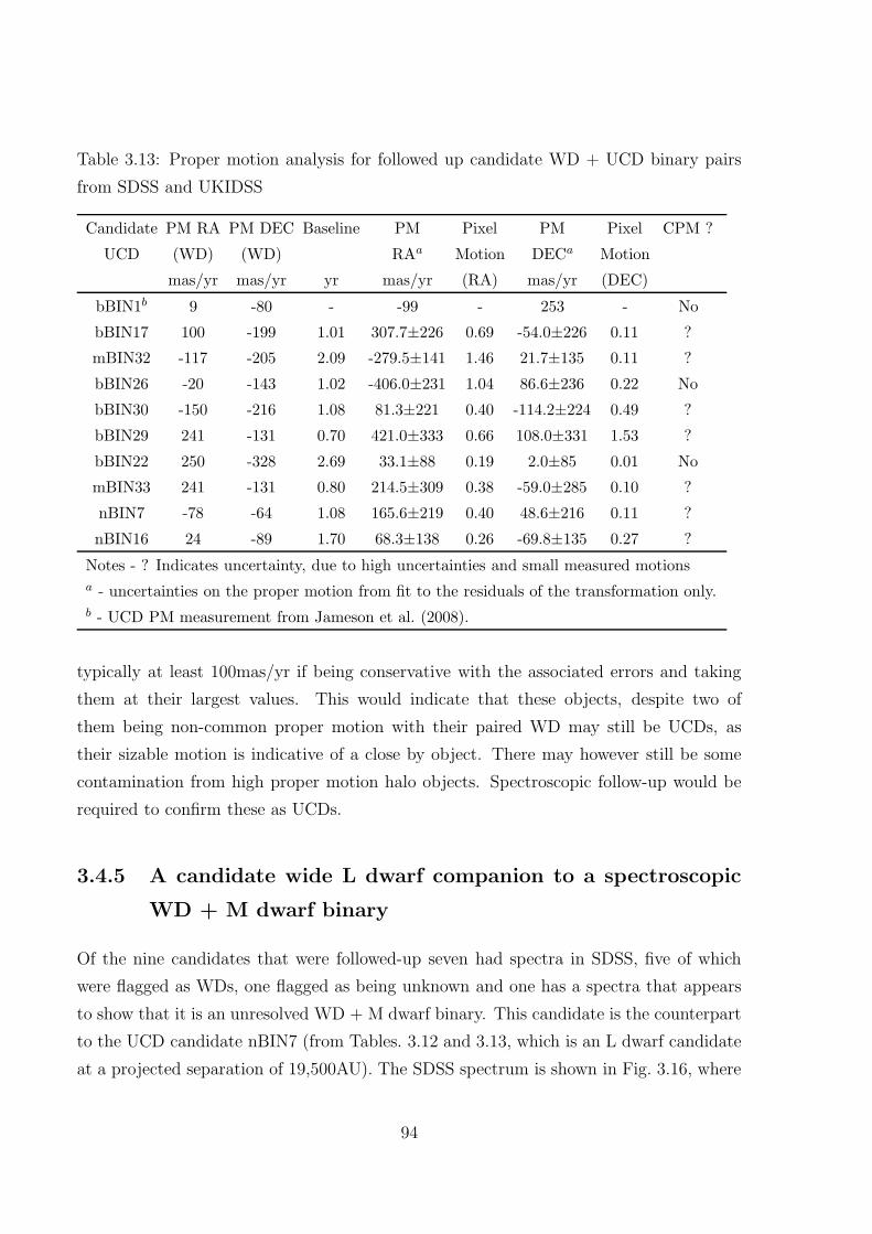
Table 3.13: Proper motion analysis for followed up candidate WD + UCD binary pairs
from SDSS and UKIDSS
Candidate PM RA PM DEC Baseline PM Pixel PM Pixel CPM ?
UCD (WD) (WD) RAa Motion DECa Motion
mas/yr mas/yr yr mas/yr (RA) mas/yr (DEC)
bBIN1b 9 -80 - -99 - 253 - No
bBIN17 100 -199 1.01 307.7±226 0.69 -54.0±226 0.11 ?
mBIN32 -117 -205 2.09 -279.5±141 1.46 21.7±135 0.11 ?
bBIN26 -20 -143 1.02 -406.0±231 1.04 86.6±236 0.22 No
bBIN30 -150 -216 1.08 81.3±221 0.40 -114.2±224 0.49 ?
bBIN29 241 -131 0.70 421.0±333 0.66 108.0±331 1.53 ?
bBIN22 250 -328 2.69 33.1±88 0.19 2.0±85 0.01 No
mBIN33 241 -131 0.80 214.5±309 0.38 -59.0±285 0.10 ?
nBIN7 -78 -64 1.08 165.6±219 0.40 48.6±216 0.11 ?
nBIN16 24 -89 1.70 68.3±138 0.26 -69.8±135 0.27 ?
Notes - ? Indicates uncertainty, due to high uncertainties and small measured motions
a - uncertainties on the proper motion from fit to the residuals of the transformation only.
b - UCD PM measurement from Jameson et al. (2008).
typically at least 100mas/yr if being conservative with the associated errors and taking
them at their largest values. This would indicate that these objects, despite two of
them being non-common proper motion with their paired WD may still be UCDs, as
their sizable motion is indicative of a close by object. There may however still be some
contamination from high proper motion halo objects. Spectroscopic follow-up would be
required to confirm these as UCDs.
3.4.5 A candidate wide L dwarf companion to a spectroscopic
WD + M dwarf binary
Of the nine candidates that were followed-up seven had spectra in SDSS, five of which
were flagged as WDs, one flagged as being unknown and one has a spectra that appears
to show that it is an unresolved WD + M dwarf binary. This candidate is the counterpart
to the UCD candidate nBIN7 (from Tables. 3.12 and 3.13, which is an L dwarf candidate
at a projected separation of 19,500AU). The SDSS spectrum is shown in Fig. 3.16, where
94

Figure 3.16: SDSS spectra of the WD candidate nBIN7.
the hydrogen Balmer lines of a DA WD are clearly visible at the blue end and features
of a cooler M dwarf, such as the VO feature at 7500A , NaI at 8200A and CaH at 7050A
can be seen at the red end of the spectrum.
Estimating spectral types of the WD and M dwarf
In order to establish the WD and M dwarf contribution to the spectra, convolved spectral
models were constructed. Template WD spectra were taken from the SDSS DR1 WD
spectroscopic catalogue of Kleinman et al. (2004) and template M dwarf spectra were
taken from Bochanski et al. (2007), who have co-added many spectra of the same spectral
type to create template spectra for M0-L0 covering the SDSS wavelength range (3800-
9100A).
The WD and M dwarf spectra were both rebinned to the same dispersion and
wavelength range as the original SDSS spectra. The WD and M dwarf components were
then individually scaled to the peak of the flux of the WD and M dwarf, respectively. The
WD was firstly normalised to the flux peak in the SDSS reference spectrum at 4000A the
M dwarf spectrum was then scaled to the peak of the flux of the M dwarf component at
8080A in the SDSS reference spectrum. Both components were then smoothed to the same
resolution as the SDSS reference spectra and finally combined together, by adding the
WD and M dwarf components. This was repeated for different combinations of DA WD
and UCD (M0-L0) and overplotted onto the original SDSS spectra for visual comparison.
95

The best fit to the SDSS spectra was found by visually inspecting the fit to the
model spectra. On first inspection the best fit to the WD comes from a DA4/5. The
WD + M dwarf spectra for a DA4 and DA5 are shown in Figs. 3.17 and 3.18. On closer
inspection to the depth and width of the Balmer lines and the depth of the features in the
M dwarf combined with the overall fit, the best fitting spectral combination is provided
by a DA4 + M4, as shown in Fig. 3.19.
To verify the spectral type of the M dwarf and check for any possible spectroscopic
peculiarities, the model DA4 was deducted from the original SDSS spectrum and spectral
ratios covering the wavelength range 3800-9000A were assessed, including the pseudo-
continuum (PC) ratios from Martın, Rebolo & Zapatero-Osorio (1996) and Martın et al.
(1999). The PC ratios use points in the spectrum that are less affected by molecular opac-
ity that cause the true stellar continuum to be suppressed, causing a pseudocontinuum.
The PC1, PC2 and PC3 ratios were used over this wavelength range (3800-9100A).
The PC1 ratio (the mean flux in the ranges 7030-7050A/6525-6550A) gave a ratio of
1.406, which corresponds to a spectral type of an M4/5 from table 3 of Martın, Rebolo
& Zapatero-Osorio (1996). The PC2 ratio (7540-7580A/7030-7050A) was measured as
1.677, indicating an M5 type. The PC3 ratio was also assessed, which is used as the
primary index for spectral typing by Martın et al. (1999). The ratio (8230-8270A/7540-
7580A) was measured as 1.148; indicating an M4 type. This verifies the M4 type that
was initially estimated from the model comparison with the convolved spectra. The M4
spectra with the DA4 model removed is shown in Fig. 3.20, with the model M4 spectra
overplotted for comparison.
An age estimate for the WD + M4 system
The spectrum of the M4 (with the WD component removed) can also be used to place a
crude age estimate on the age of the system. West et al. (2008) calculated an age-activity
relation for M dwarfs based on their Hα emission. Activity in M dwarfs has been shown
to decrease over time and suggests that it is thus limited to a finite age (Fleming, Schmitt
& Giampapa 1995; Gizis, Reid & Hawley 2002). If stars are still active they should show
prominent Hα emission at 6562A . The M dwarf spectra here (shown in Fig. 3.20), was
compared to the template spectra of active and non-active M dwarfs from Bochanski et al.
(2007) and shows no evidence of Hα emission. West et al. (2008) calculate an activity
lifetime of 4.5+0.5−1.0 Gyr for an M4 dwarf, which suggests that this system is ≥ 3.5Gyr.
96

Figure 3.17: Model DA4 WD spectra combined with M0-L0 (top to bottom) spectra (solid
lines) overplotted with the original SDSS spectra (red dotted lines) over the wavelength
range (3800-9100A).
97

Figure 3.18: Model DA5 WD spectra combined with M0-L0 (top to bottom) spectra (solid
lines) overplotted with the original SDSS spectra (red dotted line) over the wavelength
range (3800-9100A).
98
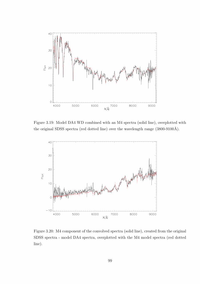
Figure 3.19: Model DA4 WD combined with an M4 spectra (solid line), overplotted with
the original SDSS spectra (red dotted line) over the wavelength range (3800-9100A).
Figure 3.20: M4 component of the convolved spectra (solid line), created from the original
SDSS spectra - model DA4 spectra, overplotted with the M4 model spectra (red dotted
line).
99

Thus if the UCD wide binary candidate is confirmed as so, through proper motion and
spectral analysis, it will have at least an independent minimum age constraint.
3.5 Summary of chapter
This chapter has presented the search for UCD companions to WDs using archival data
from SuperCOSMOS and 2MASS, including the discovery of the widest separated UCD
+ WD binary system. Also presented were a large number of candidate UCD + WD sys-
tems from SDSS (DR6) and UKIDSS (DR3). Of these 156 candidate binaries, 10 UCD
components have been followed-up with second epoch imaging to assess their proper mo-
tion. Three were found to be non-common and thus not UCD + WD binary systems.
The other seven remain uncertain due to high uncertainties associated with their mea-
surements arising from a combination of a short baseline and a small motion of the object.
One of these uncertain systems however has a spectroscopic WD + M4 primary, which
has a minimum age constraint of 3.5 Gyr, based on the non-presence of Hα in the M
dwarf spectrum and the age-activity relations from West et al. (2008). Thus if this UCD
is confirmed as such it will be add to the complement of UCDs with known ages and be
able to provide useful information for trends in properties with age. Further studies of the
WD will also allow an additional verification of the age of the system. Indeed if the WD
proves to have a high mass, it is likely to yield an age constraint to within 10% accuracy,
which would make it an ideal benchmark system.
The other candidates, along with the four systems (UCD5, 6, 7 & 8) remain uncer-
tain from the search of SuperCOSMOS and 2MASS. All require additional epoch imaging
to properly assess if their motion is common to their paired WD. Subsequent spectroscopy
of any confirmed common proper motion systems would also be needed to confirm their
nature as UCDs. The sample however looks promising for potentially finding a large
number of UCD companions to WDs at wide separations. If confirmed these will greatly
increase the number of such systems known as well as providing useful age constraints.
100

Chapter 4
Ultracool companions to Subgiants
Presented in this chapter is a search for widely separated UCD companions to subgiant
stars in the southern hemisphere through a NIR imaging survey. The observational strat-
egy, calibration and analysis is described that allows the selection of good candidate binary
systems. In addition, the followup methods, subsequent analysis and the findings so far
are summarised in the following sections.
4.1 A pilot survey of southern Hipparcos subgiants
A pilot survey was carried out to search for UCD companions to Hipparcos subgiants via
NIR imaging, using the 3.9m Anglo-Australian Telescope (AAT) and the IRIS2 instrument
(in wide field imaging mode) over an eight night run in 2005 December. The FOV allows
for wide separations to be probed with relatively short integration times, enabling a
subgiant to be efficiently imaged in three NIR filters over approximately 20 minutes per
target.
4.1.1 Selection of subgiants
The subgiant sample were selected from the Hipparcos catalogue (Perryman et al. 1997)
and as described in Pinfield et al. (2006), a publication on which I collaborated. Selected
subgiants have well measured magnitudes, parallax distances and a large number have a
constrained mass, age and metallicity from Feltzing, Holmberg & Hurley (2001) and from
Nordstrom et al. (2004), who both derive metallicity from Stromgren photometry and then
101

use stellar evolution models to infer a corresponding age. Subgiants were selected based
on their position on a MV against B −V CMD for stars with V < 13.0 and B − V > 0.6.
A parallax measurement constraint was also imposed such that π/σ ≥ 4, leading to an
uncertainty in the parallax of ≤25%. A range in MV of 2.0-4.5 was also chosen to avoid
the brightest subgiants, for which glare may become as issue when trying to image faint,
closely separated UCD companions, whose signal may be hidden by the PSF wings of
very bright subgiants, which can extend for several arcsec.
The colour cuts were defined to select against dwarfs and giant stars, as shown by the
selection boxes in Fig. 4.1, using solar metallicity isochrones from Girardi et al. (2000) as a
guide. Note that these isochrones become bluer and brighter for lower metallicity and it is
therefore possible that some contamination may arise from sub-solar metallicity giants in
the top right of the selection region. To help minimise this contamination any objects spec-
troscopically flagged as giants in the Hipparcos database were removed from the sample.
Another issue considered was interstellar reddening, that could make it difficult to sep-
arate L dwarfs photometrically from reddened background objects. Therefore subgiants
in reddened regions where galactic extinction was higher than AV > 0.3(EJ−K < 0.05)
(derived from the reddening maps of Burstein & Heiles 1982) were removed from the
sample. Areas of overcrowding were also avoided as blended point source profiles may be-
come problematic when extracting photometry. These areas included the galactic plane,
LMC, SMC and some areas where the nearest neighbouring object was <10 arcsec away.
Subgiants with small proper motions (< 40mas/yr) were also removed, as confirmation of
UCD companions will be based partially on subsequent proper motion measurements. If
a subgiant has a small proper motion it will be difficult to confirmation a UCD companion
through common proper motion over a short baseline. Finally a distance constraint of
160pc was imposed, as L and T dwarfs at distances greater than this would have apparent
brightnesses that are too faint to be detected in the exposure times that were used. This
set of selection criteria gave a target sample of 918 subgiants.
4.1.2 Simulated populations
Simulations of the expected number of UCD companions to subgiants that could be
discovered with imaging observations was presented in Pinfield et al. (2006). This was
based on a simulated disk population of subgiants. A Salpeter mass function was assumed,
with a birth rate history from Rocha-Pinto et al. (2000) and a disc scale height-age
102

Figure 4.1: Subgiant selection. (a) An MV against B − V diagram of Hipparcos stars
with V < 13.0 and π/σ ≥ 4. (b) Theoretical isochrones from Girardi et al. (2000) for solar
metallicity. Overplotted as boxed areas in both plots is the subgiant selection region.
103

relation from Just (2003). A metallicity distribution was taken from Edvardsson et al.
(1993) and UCD companions were randomly added to the simulation around 34% of the
subgiant sample (the wide binary fraction from Pinfield et al. 2006, although uncertainties
associated with this fraction were also taken into account), with separations uniformally
distributed between 1000-5000AU. An age distribution for the UCDs was derived for the
subgiant sample and a UCD mass function of a power law where α=1 (following Gizis
et al. 2001) was imposed. Lyon group models were used to derive Teff , log g and MJ
from UCD mass and age, and a J- band magnitude was calculated for the distance of
the subgiants. This simulated distance-magnitude and separation-distance distribution
is shown in Fig. 4.2 and 4.3, respectively. Also shown in 4.3 is the glare limit, which
corresponds to the minimum separation that could be imaged around a star. This was
calculated from the brightness of the object. The brighter the object the larger the PSF
wings (glare), however brighter objects are also generally closer and so separations of a
few arcsec, correspond to only a few AU at these distances. This effectively causes the
two effects to cancel each other out, creating a nearly vertical glare limit. A photometric
limit of J ≤20 was also imposed on the selection of simulated UCD companions, such that
UCD candidates could be spectroscopically followed up on an 8m class telescope. The
simulation predicts that ∼ 80+21−14 L and T dwarfs with J ≤ 20 might be detectable around
a sample of 918 subgiants within a distance of 160pc, across the whole sky. Note that
this value, obtained from simulations is indicative rather than rigorously quantitative.
4.2 The pilot survey
Imaging of a subset of the sample was taken during 2005 December 05-12 on IRIS2/AAT
in the J-, H- and Z- bands. The IRIS2 Z- band is actually very similar to the YMKO
filter used by UKIDSS, thus UCD companions were selected via their colours based on
previously described (see §2.2.2). Subgiants for this subset were selected so that they were
visible at >30◦ (airmass <2) for at least an hour during the observing time allocation.
Out of the sample of 918 subgiants, 384 were visible from the AAT during the scheduled
observing time. Targets were then prioritised according to distance, so that the closest
subgiants were higher priority, along with those that already had a well constrained mass,
age and/or metallicity.
104

Figure 4.2: Simulated distance - magnitude distribution of UCD companions to Hipparcos
subgiants from Pinfield at al. (2006). Dotted lines show the positions of the M/L, L/T and
T/Y dwarf transition. The dashed lines show the photometric limits that were employed
to simulate potential survey and followup limitations. The 2MASS photometric limit is
also shown for comparison. The simulated UCD companions are overplotted as large filled
circles.
105

Figure 4.3: Predicted separation-distance distribution of subgiant + UCD binaries from
Pinfield et al. (2006). The vertical dashed line shows the separation at which the subgiants
PSF wings are expected to extend for the sky background to be doubled in the Z- band,
thus indicating the lower limit above which the PSF wings will not significantly affect the
detection of faint companions. The other dashed lines indicate the maximum separation
covered by the IRIS2/AAT and LIRIS/WHT imagers. The dotted lines show the expected
separation range for wide binary systems to main sequence stars (1000-5000AU), including
subgiants. Overplotted as filled circles are the simulated UCD companions.
106

4.2.1 Observing strategy
The observing strategy adopted was to image around each of the subgiants by observing
two fields, one to the north of the subgiants position and one to the south, so that
the subgiant was just off the FOV. Observations made in this way also allow for wider
separations around the subgiant to be searched. A separation of 1000AU at a distance of
50-150pc corresponds to an angular separation of 7-20 arcsec. It is estimated that ∼95%
of the potential companion region around each subgiant are included when imaging in
this way. The offset amount (between the edge of the array and the position of the
subgiant) required was determined from the distance of the subgiant. The offset (in the
DEC direction) was calculated as ±231 + 12( 1000AU
Distance) arcsec (where 231′′ = half the FOV
of IRIS2). The position of the IRIS2 observing field, with respect to the subgiant is shown
in Fig. 4.4.
Over the eight night observing period 71 subgiants were imaged in the J-, H- and Z-
bands, using total exposure times of 1, 2 and 5 minutes respectively. A five point dither
pattern was used with 12s (J- and H-) and 60s (Z-) exposures at each position. The
sensitivity reached using these exposure times, with the observing conditions (average
seeing ∼1 arcsec) was J =19.0 to a 5σ detection limit.
4.2.2 Extraction and calibration of photometry
The images were reduced with the standard oracdr package for IRIS2, as described in
§3.2.1. Photometry was then extracted using the following iraf routines. The daofind
routine was used to identify stars within the image that were above a minimum detection
value of 5σ above the background value, and extended over a greater area than the full
width half maximum (FWHM) of faint stars in the image to avoid selecting cosmic rays.
This was measured by inspecting individual images using imexamine and taking the
standard deviation of the background and measuring the average FWHM for fainter stars
in individual images. A saturation limit of 25,000 counts was also imposed to avoid very
bright, saturated objects in any image.
The process of detecting objects was checked by overlaying their coordinates onto the
original image using the tvmark command. The detection limit had to be changed on one
or two occasions to strike the best balance between detection of faint stars whilst avoiding
noisy background regions. The phot routine was then used to extract photometry of the
107
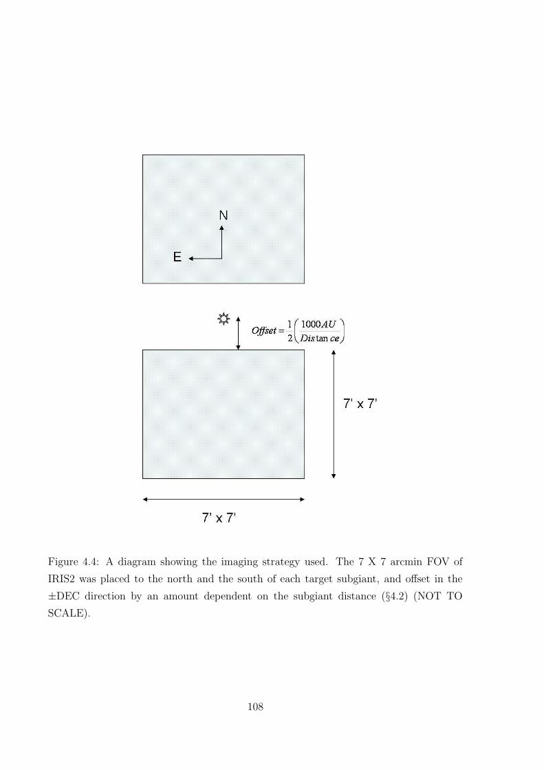
Figure 4.4: A diagram showing the imaging strategy used. The 7 X 7 arcmin FOV of
IRIS2 was placed to the north and the south of each target subgiant, and offset in the
±DEC direction by an amount dependent on the subgiant distance (§4.2) (NOT TO
SCALE).
108

objects using an aperture size of twice the FWHM (in pixels) and where the measured
photometric uncertainty was <5σ for each filter. Objects in all three filter images were
cross matched by their pixel coordinates using the tmatch routine, with a matching
radius of three pixels.
Calibrating with standard stars
To calibrate the photometry, firstly the extracted magnitudes were normalised to 1 sec-
ond exposures. This was done by adding a magnitude correction (MC), defined by the
exposure time, such that MC=-2.5log(exposuretime). An airmass curve was then derived
to determine a zero-point (ZP) as a function of the zenith distance. A0 standard stars
were observed throughout the night at different airmasses and a ZP was calculated from
the instrumental magnitude (and airmass). The starlink software gaia was used to
extract the flux (normalised to a 1 second exposure) and convert it to an instrumental
magnitude, ZP where ZP=-2.5log(flux). The corresponding airmass was calculated from
the zenith distance (obtained from the fits header) such that airmass= 1cos(ZD)
. The ZP
was then plotted for observations at different airmass to create an airmass curve by using
a least squares fit to the observed data points. An example of this shown in Fig. 4.5. This
was used to calculate a corresponding ZP for a said airmass.
An aperture correction was calculated using the true magnitude of the standard star,
as measured by the 2MASS science archive. The aperture correction, being the difference
between the true (2MASS) magnitude and the instrumental (IRIS2) magnitude. The
2MASS science archive provides magnitudes in the J- and H- bands. For the Z- band the
knowledge that A0 stars have zero colour was used to assume the Z- band magnitude to be
the same as the J- band magnitude. In addition the 2MASS magnitudes were converted
into the MKO filter system (see §2.2.2) used by IRIS2, which were calculated from the
colour relations of Carpenter (2001). For A0 stars (J − H=0), this correction was small
(+0.002 mags). The calibrated magnitudes were then calculated as Magcal=ZP-Maginst-
Aperture correction. This was repeated for each of the J-, H- and Z- bands, for each
night of observation.
Calibrating with 2MASS objects
For the nights where no standard star observations were made or only one measurement
was taken, due to bad weather causing short observing windows or the early closure of
109

Figure 4.5: An airmass curve for standard star observations taken on the first night of
observations (see §4.2.2).
the telescope, 2MASS objects in the images were used as secondary calibrators. The large
FOV allowed enough reference stars to be identified from 2MASS for the purposes of a
photometric calibration based on their J −H colour. J- and H- band images were down-
loaded from the 2MASS infrared data archive for the same area of sky as the observations.
The Starlink package astrom was then used to convert 2MASS coordinates into pixel
coordinates on the IRIS2 image, using a set of ∼10 stars for reference. The 2MASS
objects were then matched with objects in the IRIS2 image using tmatch in iraf, as
described previously. A calibration was determined by converting 2MASS magnitudes
into IRIS2 magnitudes for the J- and H- bands and using the difference in magnitude
(e.g. JIRIS2 − J2MASS), which was calculated by plotting ∆ magnitude as a function of
JIRIS2. Using a least squares fit to the data it was possible to interpolate for fainter ob-
jects visible in the IRIS2 images, that were not present in the 2MASS images. For the Z
band, ZIRIS2-J2MASS was used and plotted against J −H(2MASS). A least squares fit was
made to the data points and the difference in the magnitude at J −H=0 (the equivalent
of an A0 star) was calculated and applied to the instrumental magnitude, along with the
small (+0.002) correction to account for the differences in the filter systems. An example
of the 2MASS calibration plot is shown in Fig. 4.6.
110

Figure 4.6: A J −H against ∆ magnitude plot showing the ZP calibration using 2MASS
objects for the Z- band for one IRIS2 imaging field.
Calculating uncertainties on the magnitudes
The uncertainties associated with the calibrated magnitudes were calculated from the
errors on the instrumental magnitude, which were taken from the uncertainties measured
by iraf when using the phot routine, as measured from the flux and background values of
the images. The uncertainties on the ZP were taken from the RMS fit of the airmass curve
and were typically ±0.02-0.03 mags. Finally the uncertainty in the aperture correction
must also be taken into account. This was also taken from the RMS of the aperture
correction fit. These were all added in quadrature to give the final uncertainties on the
calibrated magnitudes.
4.2.3 Selection of good candidate systems
In order to select star-like or point source objects and avoid contamination from extended
sources (i.e. galaxies) an analysis of the shape of the objects in the images was made.
Photometry was extracted for two aperture sizes; using a radius of one pixel, and of twice
the FWHM (in pixels). For extended sources the difference in average flux between the
two apertures should be greater than for point sources. This difference (in magnitude)
111

Figure 4.7: A plot of magnitude against the difference in flux between two aperture sizes
in the J- band for objects in one image. Overplotted is the selection line (dot-dash),
where point like objects were selected if they lay below this.
was plotted against instrumental magnitude for each band (e.g. Fig. 4.7) and shows that
point and extended source objects are well separated, although it is noted that there is
some scatter at fainter magnitudes. A selection line was chosen to encompass some of this
spread but also remove objects that were clearly not point source like. Sources consistent
with being star-like are selected if they lie below this selection line.
Colour and magnitude selection
Candidate L and T dwarfs were selected from their position on a two colour diagram
and a CMD, based on previously described selections presented in §2.2.2 and §3.4, where
MJ was calculated from the measured parallax distance of the subgiant. As the Z- filter
of IRIS2 is similar to that of the Y - band filter used on WFCAM/UKIDSS, a similar
two-colour selection space was used, with an expansion to allow for slight differences in
the filter systems and errors on the colours. The expanded two-colour region is shown
in Fig. 4.8 and overlaps with the colour selection used previously. The colour-magnitude
space as presented in §3.4 was also adopted here and candidate UCDs were selected if
they met the following photometric criteria.
112

L dwarf colour and magnitude selection criteria:
0.5 ≤ J − H ≤ 1.2, 0.9 ≤ Z − J ≤ 2.0
and
11.0 ≤ MJ ≤ 15.0, MJ ≤ 8.5(J − H) + 7.0
L/T dwarf colour and magnitude selection criteria:
0.5 ≤ J − H ≤ 1.2, 0.9 ≤ Z − J ≤ 1.5
and
J − H ≤ 1.25(Z − J) − 0.65 and MJ ≥ 8.5(J − H) + 7 and MJ ≥ 13.5
T dwarf colour and magnitude selection criteria:
0.5 ≥ (J − H) ≥ 0 and Z − J ≥ 0.5
J − H ≤ 1.25(Z − J) − 0.65 and MJ ≥ 8.5(J − H) + 7 and MJ ≥ 13.5
or
0 ≥ (J − H) ≥ −0.5 and Z − J ≥ 0.5
J − H ≤ 1.25(Z − J) − 0.65 and MJ ≥ 8.5(J − H) + 7 and MJ ≥ 13.5
Objects from each field imaged were plotted onto a two-colour diagram and a CMD
and the position of candidate UCDs, with respect to MS stars (the bulk of the objects in
the image) was inspected. Sources that sat close to the MS were rejected as they were
deemed likely contaminant M dwarfs.
Whilst the selection and calibration was carried out meticulously there could still
be some sources of contamination. One source may come from cosmetic effects such
as cross talk, or from contaminant red giant stars, which exhibit similar colours to L
dwarfs. In order to minimise this all candidates were eyeballed in the J-, H- and Z- band
images to make sure they were good detections. Objects were also cross matched with
the SuperCOSMOS science archive data where I- and R- band images were inspected
to check for optical counterparts. The quoted limiting magnitude for detection in the
SuperCOSMOS SSA I band is ∼18.5, but objects around a magnitude fainter can still be
seen in the images. Objects with an R- and/or I- band counterpart such that I − J ≤3.0
were deemed not consistent with being UCD like, following the optical plus NIR colours
of late M, L and T dwarfs from Hawley et al. (2002). If an object was not detected in
113

Figure 4.8: A J − H against Y − J two-colour diagram, showing the position of main
sequence stars, M, L and T dwarfs, along with the predicted colours of very cool dwarfs
(Teff < 700K), as described in §2.2.2 and §3.4. Overplotted are the IRIS2 L and T
dwarf selection area for subgiant companions as red dashed and blue dot-dashed lines,
respectively.
the archive but was visible in the I- or R- band image, it was assumed that the I- band
magnitude was 18.5 ≥ I ≥ 19.5 and thus the I −J colour assessed from this. If there was
no I- and R- band detection then these remained good candidate UCDs.
This selection yielded 30 candidate subgiant + UCD wide binary systems, for which
the UCD candidate components consisted of 2 L dwarf, 3 L/T and 25 potential T dwarf
candidates. The details of the potential systems are shown in Fig. 4.9, where L dwarfs
are shown as red plus signs, L/T candidates as orange asterisks and T dwarfs as blue
diamonds, and are referenced in Table. 4.1.
4.3 Follow-up Observations
A follow-up program was undertaken to confirm the status of the candidate binary pairs
and the nature of the UCD candidate components. In order to confirm companions
the approach was taken to measure proper motion. The subgiants all have accurately
measured proper motions and taking second epoch images will allow the proper motion of
the UCD candidates to be calculated. Common proper motion pairs can then be searched
114

Figure 4.9: Left: A J −H against Z −J two-colour diagram, showing candidate L dwarfs
(red plus symbols), L/T candidates (orange asterisks) and T dwarfs (blue diamonds),
overplotted with the selection regions, as defined in §4.2.3 Right: A MJ against J − H
CMD of L and T dwarf candidates, symbols the same as plot on the left and overplotted
with the corresponding selection regions.
115
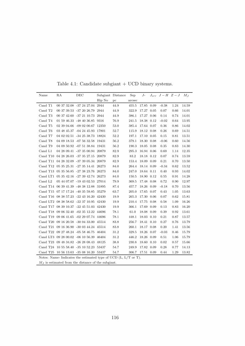
Table 4.1: Candidate subgiant + UCD binary systems.
Name RA DEC Subgiant Distance Sep J- Jerr J − H Z − J MJ
Hip No pc arcsec
Cand T1 00 37 32.08 -37 24 27.04 2944 44.9 455.5 17.85 0.09 -0.38 1.24 14.59
Cand T2 00 37 39.53 -37 20 26.79 2944 44.9 322.9 17.27 0.05 0.07 0.66 14.01
Cand T3 00 37 42.60 -37 21 10.73 2944 44.9 386.1 17.27 0.06 0.14 0.74 14.01
Cand T4 01 59 46.33 -48 40 36.85 9316 76.9 241.5 18.38 0.12 -0.02 0.64 13.95
Cand T5 02 39 04.66 -09 02 00.67 12350 53.0 385.4 17.64 0.07 0.36 0.86 14.02
Cand T6 03 48 45.37 -04 24 45.93 17801 52.7 115.9 18.12 0.08 0.26 0.69 14.51
Cand T7 04 02 02.51 -34 25 38.73 18824 52.2 197.1 17.10 0.05 0.15 0.81 13.51
Cand T8 04 09 18.53 -07 56 32.58 19431 56.2 379.1 18.30 0.08 -0.06 0.60 14.56
Cand T9 04 09 50.92 -07 51 38.84 19431 56.2 190.3 18.05 0.08 0.35 0.83 14.30
Cand L1 04 28 09.41 -37 35 00.94 20879 82.9 295.3 16.94 0.06 0.69 1.14 12.35
Cand T10 04 28 26.03 -37 35 27.15 20879 82.9 83.2 18.18 0.12 0.07 0.74 13.59
Cand T11 04 28 32.09 -37 39 05.34 20879 82.9 153.4 18.09 0.09 0.21 0.70 13.50
Cand T12 05 35 25.31 -27 35 14.41 26273 84.0 264.4 18.14 0.09 -0.34 0.62 13.52
Cand T13 05 35 56.85 -27 38 23.76 26273 84.0 247.0 18.64 0.11 0.40 0.93 14.02
Cand LT1 05 35 42.16 -27 39 42.74 26273 84.0 150.5 18.90 0.12 0.55 0.91 14.28
Cand L2 05 44 07.07 -19 43 02.53 27014 79.9 369.5 17.48 0.08 0.72 0.90 12.97
Cand T14 06 39 41.39 -48 38 12.88 31895 87.4 457.7 18.26 0.09 -0.18 0.70 13.56
Cand T15 07 17 17.24 -40 35 59.85 35279 63.7 205.0 17.65 0.07 0.43 1.05 13.63
Cand T16 08 38 57.23 -22 43 16.20 42430 19.9 265.3 17.30 0.06 0.07 0.62 15.81
Cand LT2 08 38 58.62 -22 37 10.95 42430 19.9 210.4 17.75 0.08 0.58 1.09 16.26
Cand T17 08 39 10.37 -22 45 51.03 42430 19.9 366.1 17.69 0.09 0.13 0.83 16.20
Cand T18 09 06 32.40 -02 35 12.22 44696 78.1 61.0 18.08 0.09 0.39 0.92 13.61
Cand T19 09 06 41.65 -02 29 07.74 44696 78.1 448.1 18.03 0.10 0.21 0.87 13.57
Cand T20 09 16 20.58 -30 04 33.00 45514 83.8 256.7 18.41 0.10 0.27 0.76 13.79
Cand T21 09 16 36.90 -30 03 44.24 45514 83.8 260.1 18.17 0.08 0.20 1.41 13.56
Cand T22 09 27 48.24 -05 58 46.75 46404 31.2 329.5 18.26 0.07 -0.03 0.46 15.79
Cand LT3 09 28 00.02 -06 10 56.39 46404 31.2 446.2 18.26 0.09 0.51 1.06 15.79
Cand T23 09 48 34.82 -26 28 08.43 48125 38.8 230.8 18.60 0.10 0.02 0.57 15.66
Cand T24 10 55 58.40 -35 10 52.23 53437 54.7 249.9 17.82 0.09 0.28 0.77 14.13
Cand T25 10 56 13.63 -35 08 16.20 53437 54.7 306.7 17.51 0.09 0.44 1.29 13.82
Notes: Name- Indicates the estimated type of UCD (L, L/T or T).
MJ is estimated from the distance of the subgiant.
116

for, in the same way as 2MASSJ0030− 3739 and 2MASSJ0030− 3740 were confirmed as
a WD + M9 wide binary system (see §3.3). For the T dwarf candidates the follow-up was
performed with methane filters, to assess the strength of any methane absorption, which
would indicate a T dwarf.
4.3.1 Second epoch imaging
L and early T dwarf candidates were followed-up with second epoch imaging using WF-
CAM on UKIRT, EMMI on the New Technology Telescope (NTT) and with IRIS2 on the
AAT.
WFCAM
Observations of Cand T9 and Cand T5 were taken using WFCAM/UKIRT (described
in §3.2.1). Cand T9 was imaged for a total integration time of 75 seconds, composed of
three cycles of five second exposures using a five point jitter pattern and Cand T5 for 50
seconds (10 second individual exposures) in the J- band on 2007 September 24.
The images were reduced and calibrated using the WFCAM/UKIDSS standard
pipeline (Irwin et al. 2008) and proper motions were calculated as described in §3.2.1.
Cand T5 is a potential T dwarf companion to the subgiant Hip12350, which has a proper
motion of 277.8 mas/yr (PMRA: 272.9 mas/yr, PMDEC: -51.8 mas/yr). Using 18 ref-
erence stars over a baseline of 1.78yr the proper motion measured for Cand T5 was
217±111 mas/yr, where the quoted errors are from the residuals of the coordinate transfor-
mation and from centroiding errors, which were conservatively taken as 0.5 pixels. At first
glance the motion seems common, however when the direction of motion is analysed into
the RA and DEC components (PMRA: -168±141 mas/yr and PMDEC: 137.±153 mas/yr)
which showed the pair do not share a common proper motion, even when taking into ac-
count their large uncertainties, thus this system is rejected as a real binary system.
Cand T9, is paired with subgiant Hip19431 (PM: 107.2 mas/yr, PMRA: 34.5 mas/yr,
PMDEC: 101.5 mas/yr), using 19 reference stars over the same baseline as T5, the proper
motion measured was 118.7 mas/yr (PMRA: -109±142 mas/yr, PMDEC: -45±139 mas/yr),
which showed the motion appeared not to be common. However as the movement is small
and the baseline short so it was not ruled out as a candidate system at this time.
117

EMMI
The red arm optical filter on the wide field imager of EMMI, housed on the 3.6m New
Technology Telescope (NTT) located in La Silla, Chile was used to image Cand L1, Cand
T6, Cand T10, Cand T1, Cand T12 and Cand T13 in the I- band during 2007 November
16-18. Exposure times of 900 seconds (a combination of 3 x 300 second integrations) were
taken for each candidate.
Basic data reduction, including the background, dark and bias subtraction were done
by Dr Ben Burningham. The individual (300 second) images were then cropped to remove
most of the vignetting pattern on the the chip. Cropping was done using the Starlink
figaro routine isubset to select the fully illuminated part of the image. The set of
three images were then lined up using ccdpack. Firstly the pairndf routine was used
to interactively overlay one image on top of another via the ′drag and drop′ facility, where
bright stars in the images were used as a positioning reference. This allows the offset of
each image to be calculated using the register routine, which creates a transformation
function to determine any shift, rotation or magnification in the images, with respect to
each other. The images were then transformed to the same scale, orientation and offset
using tranndf and finally median combined using makemos.
EMMI has a FOV of 9.1′ x 9.9′, with a pixel scale of 0.1665 arcsec/pixel. Proper
motions were calculated as previously described, transforming from the IRIS2/AAT co-
ordinate system into the EMMI/NTT system and vice versa to verify the proper motions
over the baseline of 1.92 yr, using an average of 18 reference stars. The proper motion
measurements of all six candidates are shown in Table. 4.2. All but one of the candidates
(Cand T13) had high associated residuals and a short baseline, leaving high uncertainties
on these measurements. For Cand T13 the motion, even considering the large associated
uncertainties appears not to be common when assessing the direction and high proper
motion of the possible subgiant companions.
IRIS2
Cand LT2 and Cand LT3 were imaged in the J- band using IRIS2/AAT during 2008
February 20-24 in seeing of 1.5-2.0 arcsec. The data were reduced using the standard
oracdr pipeline for IRIS2 and their proper motions calculated as previously described.
19 and 23 reference stars respectively were used to derive transformations over a baseline
118

Table 4.2: Proper motion measurements of candidate L and early T dwarfs.
Candidate SG PM SG PM 2nd epoch Baseline UCD PMa UCD PM a CPM?
RA DEC instrument yr RA DEC
Cand T5 272.9 -51.8 WFCAM 1.78 -168±141 137±153 No
Cand T9 34.5 101.5 WFCAM 1.78 -109±142 -45±139 ?
Cand T10 51.6 -117.0 EMMI 1.92 18±130 28±125 ?
Cand L1 54.6 -117.0 EMMI 1.92 -92±127 2±123 ?
Cand T6 42.2 -20.6 EMMI 1.92 -37±120 -36±120 ?
Cand T11 51.6 -117.0 EMMI 1.92 37±119 22±127 ?
Cand T13 23.5 -217.9 EMMI 1.92 -94±121 148±122 No
Cand T12 23.5 -217.9 EMMI 1.92 -52±122 -64±124 ?
Cand LT2 -268.3 424.1 IRIS2 2.2 -37±106 -1±104 No
Cand LT3 -232.8 -65.2 IRIS2 2.2 -15±107 -19±106 No
Notes: SG - Subgiant.
? Indicates uncertainty, due to large errors and small measured motions
a - uncertainties on the proper motion from fit to the residuals of the transformation.
of 2.2yr. Cand LT2 had a measured proper motion of PMRA: -37±120 mas/yr and
PMDEC: -1±104 mas/yr, which is consistent with a zero motion and not consistent
with the proper motion of its possible subgiant companion Hip42430, which has a sizable
measured proper motion of PMRA: -268.3.8 mas/yr and PMDEC: 424.1 mas/yr. Cand
LT3 also has a small motion of PMRA: -15 ±107 mas/yr, PMDEC: -19±106 mas/yr, which
is much smaller than the motion measured for its possible subgiant companion (Hip46404,
which has a proper motion of PMRA: -232.8 mas/yr and PMDEC: -65.2 mas/yr). These
two candidates were considered non-common proper motion objects and thus not binary
systems.
The proper motion of all candidates followed-up are summarised in Table. 4.2.
4.3.2 Methane imaging
The T dwarf spectral type is defined (and classified) by the presence of strong methane
absorption in their spectra. This shows up strongly in the NIR and is most prevalent
in the H- band over the wavelength range 1.5-1.8µm. The strength of the methane
absorption becomes stronger with later spectral type (Burgasser et al. 2003a). The
119

Figure 4.10: Plot from Tinney et al. (2005) showing the position of the methane filters;
CH4s and CH4l as dashed green and blue lines respectively, with comparison to the
H- band of IRIS2 (dotted line). Also overplotted are the spectra from an L7 and a T5
dwarf (red solid lines, normalised for clarity) from Burgasser et al. (2004) and Leggett et
al. (2001).
strong methane absorption is unique to T dwarfs and thus serves as a tool to distinguish
them from other stars. Differential imaging in and out of the methane absorption was
chosen for this reason, to test if the T dwarf candidates were genuine T dwarfs. A set
of filters based on the position of the main methane feature in the H- band were used,
following the method of Tinney et al. (2005). The two filters used are CH4s centred on
1.57µm, where there is no methane absorption and CH4l, centred on 1.69µm where the
methane absorption is strong. The position of the filters, with respect to the H- band
filter of IRIS2 and the spectra of a mid T and a late L dwarf are shown in Fig. 4.10.
The difference in flux between the two filters i.e. the CH4s − CH4l colour are measured
and compared to the that for main-sequence stars and known T dwarfs. Mid to late T
dwarfs have CH4s−CH4l < −0.5, whereas main-sequence stars have neutral colours. The
CH4s−CH4l colour for main-sequence stars and L and T dwarfs are shown in Fig. 4.11.
Also seen is a slight reddening of the methane colour for late M and L dwarfs and a sharp
blue-ward turn for mid T dwarfs.
120
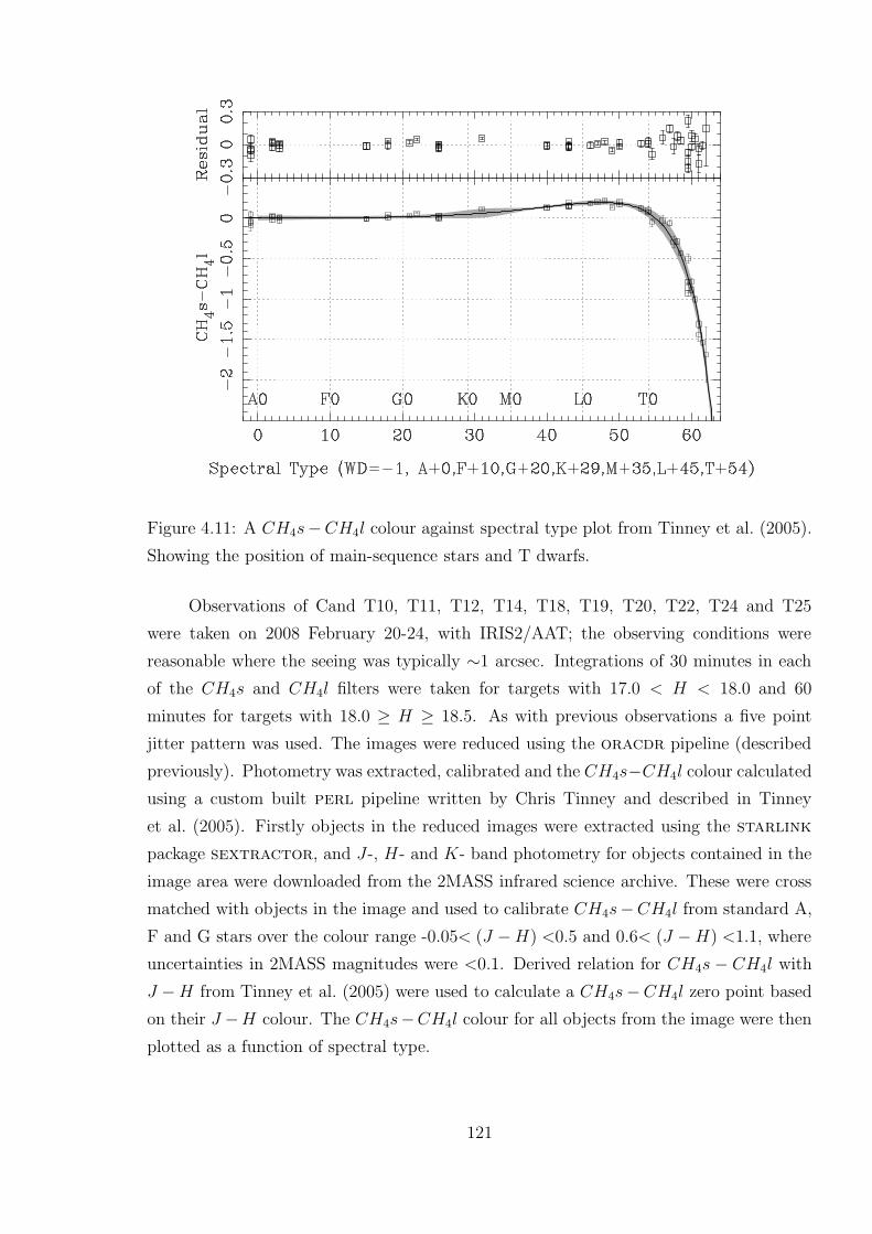
Figure 4.11: A CH4s−CH4l colour against spectral type plot from Tinney et al. (2005).
Showing the position of main-sequence stars and T dwarfs.
Observations of Cand T10, T11, T12, T14, T18, T19, T20, T22, T24 and T25
were taken on 2008 February 20-24, with IRIS2/AAT; the observing conditions were
reasonable where the seeing was typically ∼1 arcsec. Integrations of 30 minutes in each
of the CH4s and CH4l filters were taken for targets with 17.0 < H < 18.0 and 60
minutes for targets with 18.0 ≥ H ≥ 18.5. As with previous observations a five point
jitter pattern was used. The images were reduced using the oracdr pipeline (described
previously). Photometry was extracted, calibrated and the CH4s−CH4l colour calculated
using a custom built perl pipeline written by Chris Tinney and described in Tinney
et al. (2005). Firstly objects in the reduced images were extracted using the starlink
package sextractor, and J-, H- and K- band photometry for objects contained in the
image area were downloaded from the 2MASS infrared science archive. These were cross
matched with objects in the image and used to calibrate CH4s−CH4l from standard A,
F and G stars over the colour range -0.05< (J − H) <0.5 and 0.6< (J − H) <1.1, where
uncertainties in 2MASS magnitudes were <0.1. Derived relation for CH4s − CH4l with
J − H from Tinney et al. (2005) were used to calculate a CH4s−CH4l zero point based
on their J −H colour. The CH4s−CH4l colour for all objects from the image were then
plotted as a function of spectral type.
121

T dwarfs should have colours CH4s − CH4l < −0.2 (Tinney et al. 2005), however
there is a large amount of scatter for magnitudes fainter than CH4s > 18.0, as can
be seen in Fig. 4.12. Thus a confident detection of a T dwarf should exhibit colours
CH4s − CH4l < −0.2 and sit outside of the region of scatter. Cand T18, Cand T19,
Cand T24 and Cand T25 all showed CH4s − CH4l > 0.1, which is consistent with the
colours of main-sequence stars. The differential methane imaging (CH4s − CH4l against
CH4s) colour-magnitude diagram for Cand T18 is shown in Fig. 4.12, as an example.
Overplotted are other objects in the image for comparison, where it can be seen that
the candidate is likely a contaminant main-sequence object and is thus considered not
to be a T dwarf. Additionally in the FOV of Cand T18, two objects showed extreme
CH4s−CH4l colours (<-0.5) and would be typed as T7 and T8 by the pipeline. However
on closer inspection of the images one of these objects sits in an area affected by cross
talk and the other at the same location as a bad pixel in the CH4s image. Their colours
were thus deemed unreliable.
Solutions were not possible for Cand T10, T11, T12 and T20, due to one or more of
the following factors; the target could not be resolved due to an insufficient signal-to-noise
or the images were affected by cloud causing diffraction rings, thus creating an uneven
background level that made it impossible to extract reliable photometry. The T dwarf
candidate in these images was visually inspected to see if a noticeable change in brightness
in the CH4s band compared with the CH4l could be seen, indicating the presence of strong
methane, however none of the candidates showed a convincing difference in brightness and
are considered likely not to be T dwarfs, but can not be ruled out by this crude estimation.
There were two objects, Cand T14 and Cand T22, that were typed as early T dwarfs,
T0.9±1.4 and T0.5±1.5 respectively. While their CH4s−CH4l colours (-0.01±0.07 and -
0.01±0.14) are not convincingly strong detections of methane (compared to main-sequence
stars) they can not be ruled out with this data, since their colours lie in the range 0.1 <
CH4s − CH4l < −0.2 and might yet be shown to be T dwarfs. It is likely that they are
not T dwarfs but require additional follow-up to confirm their nature.
122

Figure 4.12: A CH4s−CH4l against CH4s CMD for Cand T18 (indicated with an arrow),
and an estimated spectral type that the program calculates based on the CH4s − CH4l
verses spectral type relation from Tinney et al. (2005) (shown in the insert at the bottom
right of the figure). Also shown are all other stars in the 7.7′ x 7.7′ FOV imaged by IRIS2,
providing a comparison to the position of the main-sequence. Two objects with ′extreme′
CH4s − CH4l colours are also shown as squares (see §4.3.2).
123

4.4 Discussion
Of the 30 subgiant + UCD candidate binary systems from this pilot survey, ten were
followed-up with second epoch imaging. Four of the ten systems were rejected as non
common proper motion binaries and six remain uncertain due to small motions and large
associated uncertainties on those motions (on average ∼120 mas/yr). What is needed in
order to better evaluate their binary nature is an additional epoch, over a longer baseline or
with a smaller spatial resolution and higher signal-to-noise measurement. Ten candidate
systems were also followed-up with methane imaging. Four of these were confirmed as not
being T dwarfs and were rejected as subgiant + T dwarf binary systems and six remain
uncertain due to low signal-to-noise data. For these six additional methane imaging
or spectral follow-up on an 8m class telescope is required to determine if they are real
subgiant + UCD binary systems.
There are two candidates that, despite their non-common proper motion status still
showed a potentially significant motion (Cand T5 and Cand T13). If their motion is real
(or is of low significance when compared to the large 1σ uncertainties), then they are either
close by T dwarfs or background M dwarfs (with scattered colours) with a space velocity
of ∼200km/s. It is likely however, that the latter is the case. The expected number of field
T dwarfs (not binary companions) in the IRIS2 survey area was assessed using identified
mid-late T dwarfs (≥T4) from the UKIDSS LAS DR1 and DR2 coverage. Pinfield et al.
(2008) analysed the number of ≥T4 dwarfs in the UKIDSS LAS DR2 coverage, which
is effectively complete down to J≤19. This was compared to the subgiant survey area,
which probes out to similar magnitude limits. They find 17±4 mid-late T dwarfs in the
280 degree2 coverage of UKIDSS DR2. This suggests that a T dwarf should be found
in every 16.5+4.5−3.2 degree2 of sky. The sky coverage for each subgiant was calculated as
0.0335 degree2 (15.73 x 7.7 arcmin around each subgiant), thus for the pilot survey of 71
subgiants this equates to 2.4 degree2 of sky. One would therefore expect to find 0.15+0.03−0.04
≥T4 field dwarfs in the sky coverage of the pilot survey. This suggests that a field T
dwarf should only be found once for every ∼490 subgiants imaged. Thus the chance of
finding a mid-late T dwarf that is not a companion in the imaging survey is very small,
Cand T5 and Cand T13 are hence more likely to be background objects.
The remaining ten candidates were unable to be followed-up due to their observabil-
ity during the follow-up time awarded. The best candidate is T1, which has the bluest
J −H colour and the reddest Z−J colour of the sample. This object has been prioritised
124

for near future methane and second epoch imaging. A table summerising the results of
the follow-up program are shown in Table. 4.3.
The number of subgiants with UCD companions predicted by Pinfield et al. (2006)
over the whole sky is 80+21−14 systems. Evaluating the clean sample of 918 subgiants suggests
that one in eleven should have a UCD companion. For the 71 subgiants observed during
this pilot survey, which represents 7% of the total sample, the Pinfield et al. (2006)
simulations, suggest that six systems could be found. As a large number of the candidate
systems (22 out of the 30) are uncertain it is not possible to support nor confirm the
simulated predictions, but it seems likely that several of the remaining candidates could
prove to be genuine in the future.
125

Table 4.3: The status of UCD candidates (confirmed or not).
Candidate Followup Confirmation
type of UCD?
Cand T1 No ?
Cand T2 No ?
Cand T3 No ?
Cand T4 No ?
Cand T5 PM No
Cand T6 PM ?
Cand T7 No ?
Cand T8 No ?
Cand T9 PM ?
Cand L1 PM ?
Cand T10 Met Imaging/PM ?
Cand T11 Met Imaging/PM ?
Cand T12 Met Imaging/PM ?
Cand T13 PM No
Cand LT1 No ?
Cand L2 No ?
Cand T14 Met Imaging ?
Cand T15 No ?
Cand T16 No ?
Cand LT2 PM No
Cand T17 No ?
Cand T18 Met Imaging No
Cand T19 Met Imaging No
Cand T20 Met Imaging ?
Cand T21 No ?
Cand T22 Met Imaging ?
Cand LT3 PM No
Cand T23 No ?
Cand T24 Met Imaging No
Cand T25 Met Imaging No
Notes - ? Indicates uncertainty,
due to a non measurement or large
uncertainties on the measurements.
126

Chapter 5
Ultracool companions to
main-sequence stars
A search for UCD companions to main-sequence stars was carried out and presented in
Pinfield et al. (2006). Two of these new systems identified were subsequently followed-up
with spectroscopy to confirm the nature of the UCD component here, and confirm their
usefulness as benchmark objects. Section 5.1 summarises the selection of common proper
motion binary systems from Pinfield et al. (2006) (in which I collaborated), and sections
5.2-5.4 present the new spectroscopic analysis of two of the candidates.
5.1 Selection of Hipparcos main-sequence + UCD
wide binary systems
Main-sequence stars within 50pc were selected from the Hipparcos catalogue covering
areas across the whole sky, omitting the galactic plane (|b| < 30). They include stars in
the range 0<MV <10 and -1.4<V<13.25 for early A to early M spectral types, totalling
to a sample of ∼40,000 Hipparcos stars. These stars were then cross matched with the
2MASS infrared data archive and UCD companions were searched for using a cone search
with a radius equal to a separation of 5000 AU, at the parallax distances of the stars,
out to a maximum of 300 arcsec separation (the Gator search limit). The search is
thus incomplete (out to separations of 5,000 AU) for distances < 16.67 pc. Colour and
magnitude constraints were also imposed, selecting UCD candidates if they had J −K ≥
1.1, J ≤ 16.1 and where either no optical counterpart exists in the USNO catalogue
127
(where 2MASS can cross reference the USNO data) or if the optical constraint yielded
R−K ≥ 5.5 (as described in §2.2.1). Objects were then visually inspected in images from
2MASS, SuperCOSMOS (I- and R- bands) and SDSS (DR4) where available, to ensure
there was no contamination from image artifacts.
An absolute magnitude (MJ) was calculated for the candidate UCDs by assuming
they are at the same distance as their paired Hipparcos primary. This was used to plot
candidates on a J−H against MJ CMD, where a selection region was defined using known
L dwarfs as described in §3.2. Sixteen candidate systems were identified in this way and
are shown in Table. 5.1 and Fig. 5.1 as filled circles. Five of these were previously identified
by Kirkpatrick et al. (2001) and Wilson et al. (2001) (Cand 3, 4, 5, 12 and 14) and are also
shown as overplotted circles on Fig. 5.1. For the remaining candidates, five have SDSS
measurements (Cand 2, 6, 8, 9 and 10), and Cand 13 and Cand 16 have SuperCOSMOS
measurements. All showed colours consistent with L dwarfs when compared to the colours
presented in Fan et al. (2001) and Hawley et al. (2002).
Proper motions were calculated where possible by measuring the motion between
the 2MASS first epoch and SDSS or SuperCOSMOS second epoch images. For one of
the candidate systems (Cand 2) the baseline was only ∼0.27yr, which is too short for an
accurate proper motion to be calculated. Cands 8, 10, 13 and 16 however have longer
baselines of 2.0, 6.1, 5.7 and 14.9 yr, respectively so their motions were measurable. Proper
motions were thus calculated using the geomap and geoxytran routines in iraf, as
previously described in §3.2.1 using an average of 10-15 reference stars. Residuals of the
transformations were typically 0.2-0.3 arcsec and centroiding accuracies were typically
±0.1-0.3 arcsec. Proper motions were derived using the full range of epochs available
(first epoch J-, H- and K- band and second epoch r-, i- and z- bands), giving an overall
uncertainty of 0.2-0.4 arcsec. The corresponding proper motions are shown on a vector
point diagram in Fig. 5.2. Cand 8, which has a relatively short baseline (2yr) has large
associated uncertainties, however Cands 10, 13 and 16 show a consistent motion with
their primaries and were thus identified as common proper motion binary systems.
128

Figure 5.1: Top: MJ against J −K CMD for candidate L dwarf companions to Hipparcos
stars, where MJ is estimated using the distance of the Hipparcos primary star. Bottom:
A distance - separation plot for the candidate main sequence + L dwarf binary systems.
Filled circles are objects that pass the photometric criteria defined for L dwarfs as de-
scribed in §5.1. Overplotted with circles and diamonds are previously confirmed systems
and systems with a measured common proper motion, respectively. Also overplotted is
the L dwarf separation range 1000-5000 AU (dashed lines).
129

Table 5.1: Widely separated main sequence + L dwarf candidate systems.
Cand Primary Primary L cand 2MASS ID J J − K MJ D Sep
name SpT pc AU
Cand 1 Gl 87 M1.5 2MASS J02124236+0341004 14.70±0.03 1.32 14.62 10.4 5000
Cand 2 HD 74150 K0III-IV 2MASS J08444996+5532121 14.70±0.04 1.21 11.55 42.7 865
Cand 3 Gl 337AB G9V/G9V 2MASS J09121469+1459396 15.51±0.08 1.47 13.95 20.5 946
Cand 4 HD 89744 F7IV-V 2MASS J10221489+4114266 14.90±0.04 1.29 11.95 39.0 2409
Cand 5 Gl 417 G0V 2MASS J11122567+3548131 14.58±0.03 1.86 12.90 21.7 1997
Cand 6 HD 102124 A4V 2MASS J11451802+0814414 15.47? 1.45 12.65 36.6 1842
Cand 7 HD 107325a K2III-IV 2MASS J12201925+2636278 15.83±0.16 1.28 12.42 48.1 2102
Cand 8 HD 116012 K2V 2MASS J13204427+0409045 15.25±0.05 1.62 12.82 30.5 2069
Cand 9 Gl 512.1 G5V 2MASS J13282546+1346023 15.84±0.16 1.48 14.55 18.1 848
Cand 10 HD 120005b F5 2MASS J13460815+3055038 15.46±0.06 1.25 12.20 44.9 4691
Cand 11 Gl 527Aa F6IV 2MASS J13471545+1726426 15.94±0.20 1.61 14.97 15.6 664
Cand 12 Gl 584AB G0V/G3V 2MASS J15232263+3014562 16.06±0.10 1.71 14.71 18.6 3635
Cand 13 Gl 605 M0 2MASS J15575569+5914232 14.32±0.03 1.20 11.76 32.5 3871
Cand 14 Gl 618.1a M0V 2MASS J16202614-0416315 15.28±0.05 1.69 12.88 30.3 1027
Cand 15 Gl 694.1A F5IV-V 2MASS J17420515+7208002 15.73? 1.54 14.01 22.0 1558
Cand 16 HD 216405c K1/K2V 2MASS J22530539-3751335 15.93±0.08 1.23 12.55 47.4 4950
aVariable star. bSpectroscopic binary. cDouble/multiple star.
?: 95% confidence upper limit.
130

Figure 5.2: A vector point diagram of the four candidate main-sequence + L dwarf com-
mon proper motion systems. The primary (Hipparcos) stars are shown as filled circles and
the L dwarf candidates are shown as filled squares. Cand 8, with its large uncertanties is
plotted as open symbols. Each pair are joined with a line for clarity.
5.2 Spectroscopic follow-up observations
Spectra were taken of Cand 10 and 13 with the Long-slit Intermediate Resolution Infrared
Spectrograph (LIRIS) on the 4.2m William Herschel Telescope (WHT), part of the Isaac
Newton Group of telescopes on La Palma during 2006 January 18-19. The wavelength
range of 0.9-2.3µm was measured, which covers the Z- to K- bands, however it is split
into two ranges, corresponding to the ZJ (0.9-1.5µm) and HK (1.4-2.4µm) grisms. For
Cand 13 a total exposure time of 10 minutes in ZJ and 40 minutes in HK were obtained
by nodding along the slit in an “ABBA” pattern. Cand 10 was observed with the HK
grism only with a total exposure time of 30 minutes.
5.2.1 Reduction and extraction of data
The spectra were reduced and extracted in the same way as described in §3.3.1, including
flatfielding, using dome flats and the removal of bad pixels. The A and B position data
were median combined to create a single A and B pair and were differenced to create a pos-
itive (A-B) and negative (B-A) spectrum. They were extracted using the apall routine
131

Figure 5.3: The ZJ spectrum of Cand 13.
in iraf and wavelength calibrated using a Xenon arc lamp for the ZJ spectra, and both a
Xenon and Argon lamp for the HK spectrum. The reference wavelength of the features in
each spectrum were taken from the LIRIS/WHT web pages (www.iac.es/project/LIRIS).
The spectra were flux calibrated using an F0V star for Cand 13 and an F2V star for Cand
10. The flux standard spectra were normalised to ∼1 and divided into the spectrum,
which was then multiplied by a smoothed blackbody spectrum with the same tempera-
ture as the flux standard (7020K and 6750K for an F0V and an F2V, respectively). The
positive and negative extracted and calibrated spectra were then median combined. The
resulting spectra for Cand 13 are shown in Figs. 5.3 and 5.4 and Cand 10 in Fig. 5.5.
132

Figure 5.4: The HK spectrum of Cand 13.
Figure 5.5: The HK spectrum of Cand 10.
133

5.3 Spectral classifications
The spectral type of Cand 10 and 13 were calculated using spectral ratios, equivalent
widths of the KI lines (in ZJ) and by comparison to template spectra of late M and early
L dwarfs.
5.3.1 Cand 13
Spectral ratios
Cand 13 has full spectral coverage from 0.9 to 2.3µm and was analysed using spectral
ratios available from the literature covering this wavelength range. For the ZJ spectra the
J-FeH and H2OA ratios from McLean et al. (2003), the FeH and H2OI ratios from Slesnick,
Hillenbrand & Carpenter (2004) and the H2OA ratio from Reid et al. (2001a) were used
to calculate a spectral type for Cand 13 in the range M8-L2. In the HK spectra the H2OB
and H2OD ratios from McLean et al. (2003) and Reid et al. (2001a) were considered as
well as the H2O2 ratio from Slesnick, Hillenbrand & Carpenter (2004). These ratios are
also consistent with the spectral type range indicated by the ZJ spectra. The parameters
of each of the ratios used, including their wavelength, bandwidth, their calculated values
and corresponding spectral types are shown in Table. 5.2 and indicate a spectral type of
L0±2.
Equivalent widths
Equivalent widths of the KI lines in the ZJ band were calculated as described in §3.3.1,
where the feature program in idl was used to interactively determine the width of the
feature by selecting points in the pseudocontinuum at either side of the KI line along with
the maximum depth of the feature. This method was repeated ∼30 times for each line, by
measuring the width at different points along the continuum. The equivalent width was
calculated from the median value of the measurements and the error from the standard
deviation. For KI lines at 1.168, 1.177, 1.243 and 1.254µm these were calculated and
compared to the relation between equivalent width and spectral type from McLean et al.
(2003). For the KI features at 1.168, 1.177 and 1.254µm these were all consistent with a
spectral type of M8/9 and the width of the KI feature at 1.243µm is consistent with an
M9/L0 type. The measurements, standard deviation and corresponding spectral type for
each line are shown in Table. 5.3.
134

Table 5.2: Spectral ratios for Cand 13
Spectral feature Ratio Reference Bandwidth Value SpT
µm
J-FeH 1.200/1.185 McLean ′03 0.004 0.865 M8-L2
H2OA 1.343/1.313 McLean ′03 0.004 0.685 L0±0.6
FeH 1.200/1.230 Slesnick ′04 0.013 0.854 M9.3±0.6
H2OI 1.340/1.300 Slesnick ′04 0.010 0.703 M8.8±1
H2OA 1.340/1.290 Reid ′01 0.004 0.698 L0±1
H2OB 1.456/1.570 McLean ′03 0.004 0.732 M9
H2OC 1.788/1.722 McLean ′03 0.004 0.659 L2.9±1.8
H2OD 1.964/2.075 McLean ′03 0.004 1.020 M9±0.8
H2OB 1.480/1.600 Reid ′01 0.020 0.782 L1.2±1
H2OD 2.000/2.160 Reid ′01 0.020 0.830 M8/9
H2O2 2.040/2.150 Slesnick ′04 0.010 0.883 L0±0.5
Table 5.3: Equivalent widths for Cand 13
Equivalent width Median Standard SpT
wavelength value deviation
1.168 4.747 0.668 M8/9
1.177 7.438 0.949 M8/9
1.234 7.025 1.680 M9/L0
1.254 5.254 1.646 M8/9
135

Comparison to template spectra
Template spectra of late M and early L dwarfs were used as a visual comparison to the
spectra of Cand 13 in the ZJ and HK spectra. Template spectra of an M7 (VB8), M8
(VB10), M9 (LHS2924), L0.5 (2MASSJ0746), L1 (2MASSJ1439) and L2 (KELU 1) were
obtained from the Infrared Telescope Facility SpeX spectral library (http://irtfweb.ifa.
hawaii.edu/ spex/WebLibrary/) from Cushing, Rayner & Vacca (2005). The template
spectra were broadened to the instrumental resolution of the observed spectra and re-
binned to the same dispersion. Finally the spectra were normalised to ∼1 at 1.26µm
in ZJ and at 1.64µm in HK. The spectra were then overplotted for direct comparison.
The ZJ spectra is plotted in Fig. 5.6 and the best fit comes from an M8/M9. The HK
spectra (shown in Fig. 5.7) is best fit by an M9/L0 type, both of which are consistent with
the spectral ratio and equivalent width measurements. In addition MJ was calculated as
MJ=11.76 from the distance of the primary star, which is in agreement with a spectral
type of M9/L0 type (using the spectral type-MJ relation from Dahn et al. 2002) and is
also consistent with the spectral types calculated from the other methods considered here.
Thus the estimated spectral type for Cand 13 or Gl 605B (as is here confirmed) is L0±2.
5.3.2 Cand 10
Spectral ratios
The wavelength range covered for Cand 10 is only 1.4-2.3µm (HK). The spectral ratios
used to estimate Cand 13 in this range were also used here. The H2O ratios from McLean
et al. (2003) were calculated as 0.677 for the H2OB ratio, indicating an L4 type. H2OC
gave a ratio of 0.605 and a corresponding spectral type of L5 and H2OD gives a ratio of
1.021, suggesting an M8±0.8 type. The H2OB and H2OD ratios from Reid et al. (2001a)
were calculated as 0.865 and 0.934 with spectral types M9±1 and M8, respectively. The
final spectral ratio considered, the H2O2 from Slesnick, Hillenbrand & Carpenter (2004),
gave a ratio of 0.887 which corresponds to an L0±0.5 type. All the estimated spectral
ratios of Cand 10 are shown in Table. 5.4.
136

Figure 5.6: The ZJ spectrum of Cand 13 (Black), overplotted (in red) by template spectra
(from top to bottom) of an M7, M8, M9, L0.5, L1 and L2 type from Cushing, Rayner &
Vacca (2005).
137

Figure 5.7: The HK spectrum of Cand 13 (Black), overplotted (in red) by template spectra
(from top to bottom) of an M7, M8, M9, L0.5, L1 and L2 type from Cushing, Rayner &
Vacca (2005).
138

Table 5.4: Spectral ratios for Cand 10
Spectral feature Ratio Reference Bandwidth Value SpT
µm
H2OB 1.456/1.570 McLean ′03 0.004 0.677 L4
H2OC 1.788/1.722 McLean ′03 0.004 0.605 L5
H2OD 1.964/2.075 McLean ′03 0.004 1.021 M8±0.8
H2OB 1.480/1.600 Reid ′01 0.020 0.865 M9±1
H2OD 2.000/2.160 Reid ′01 0.020 0.934 M8
H2O2 2.040/2.150 Slesnick ′04 0.010 0.887 L0±0.5
Comparison to template spectra
The HK spectrum of Cand 10 was also compared directly with the template spectra. This
was again done by broadening and re-binning to the dispersion of the observed spectra,
then normalising to ∼1 at 1.64µm. The best fit comes from an L1-L2 type, as shown in
Fig. 5.8. It should be noted that the spectra for Cand 10 is quite noisy and the estimation
of types L4 and L5 and should be taken with caution. Indeed for an L4/L5 type the UCD
would have to be much closer, at nearly half the distance of the primary (calculated from
the spectral type, absolute magnitude relations of Dahn et al. 2002) . Tentatively the
spectral type of Cand 10 is estimated as L0±2. In addition MJ was calculated as MJ=12.2
and is in agreement with a spectral type of L1 (as calculated from the distance of the
primary star). Thus Cand 10 or HD120005C is spectroscopically typed as an L0±2 UCD.
5.4 Parameters of the systems
5.4.1 Gl605
The primary star for Gl605 has a spectral type of M0V, however no information about
the age or metallicity is available from the literature. A spectrum is also unavailable
and thus any limits on the age of the system can not be placed. If a spectrum were
available then the presence of the Hα emission feature at 6562A could be assessed in
relation to age. West et al. (2008) presented an activity-age relation for M dwarfs and
suggest that for an M0, the activity lifetime is 0.8±0.6 Gyr. Over this activity lifetime Hα
should appear as a strong emission feature. While this would not represent a particularly
139

Figure 5.8: The HK band spectrum of candidate 10 (Black), overplotted (in red) by
template spectra (from top to bottom) of an M7, M8, M9, L0.5, L1 and L2 type from
Cushing, Rayner & Vacca (2005).
140

accurate constraint on the age it would give an indication if the pair were older or not
than ∼ 1Gyr. If the M0V primary were indeed >1 Gyr the Lyon group DUSTY and
COND models suggest a Teff<2200K, log g ∼5.3 dex and mass ∼0.072M�. It is also
possible to calculate a metallicity value for the M dwarf primary using the relations of
Bonfils et al. (2005), who find that metallicity in M dwarfs can be well defined from the
relation between MK and V −K, where MK is between 4.0 and 7.5 and V −K is between
2.5 and 6.0. The V and K magnitudes along with a parallax distance have been measured
for Gl605A from the TYCHO2 and 2MASS catalogues and the distance was measured
by Perryman et al. (1997). They give an MK=4.58 and V − K=3.26, which indicates an
Fe/H = -0.25±0.2 dex. If the M dwarf were metal poor, then it would be an indication of
an older disk population, however for this M dwarf no such age constraint can be placed,
thus this UCD does not make an ideal benchmark object.
5.4.2 HD120005
The primary component of the binary system containing HD120005C is a spectroscopic
binary F5V star system and has been included in various attempts to calculate age and
metallicity constraints for main sequence F type stars. Feltzing, Holmberg & Hurley
(2001) calculate a metallicity of 0.11±0.16 dex, based on Stromgren photometry and
derive an age of 2.345±0.808 Gyr, which they calculate based on the rapid stellar evolution
algorithms of Hurley, Pols & Tout (2000).
Metallicity constraints have also been derived by Nordstrom et al. (2004), who calcu-
late [Fe/H] =-0.06±0.12 dex, where they too use Stromgren photometry from Edvardsson
et al. (1993) and relations of Schuster & Nissen (1989) to calculate [Fe/H]. Marsakov &
Shevelev (1995) also derive a metallicity of 0.05 dex, from the Stromgren photometry of
Hauck & Mermilliod (1985), which is consistent with the value of Nordstrom et al. (2004)
to within their quoted uncertainties (0.12 dex). This suggests that HD 120005 is around
solar metallicity. However they also derive an age of 2.78 Gyr from the Yale isochrones
(Green, Demarque & King 1987), which is consistent with that of Feltzing, Holmberg
& Hurley (2001). There is an additional derived age and metallicity available from the
catalogue of age-metallicity relations for nearby stars from Ibukiyama & Arimoto (2002),
who derive an age of 4.03 Gyr using newer Yonsei-Yale isochrones from Yi et al. (2001)
and a derived [Fe/H] of -0.09 dex from the Stromgren photometry of Hauck & Mermilliod
(1998). Conservatively, it can be estimated that the age of HD120005C is thus 2-4 Gyr.
141

The Lyon DUSTY (Chabrier et al. 2000c; Baraffe et al. 2002) and COND (dust-
free Allard et al. 2001; Baraffe et al. 2003) models (with solar metallicity) were used to
calculate a corresponding mass, Teff and log g for HD120005C, taking an age estimate of
2-4 Gyr. Although L dwarfs have dusty atmospheres, using the dust-free COND models
provides an indication of the uncertainties that may be expected to result from different
treatments of dust. The DUSTY models suggest that for an age of 2 Gyr and MJ=12.2
(as calculated from the apparent J- band magnitude and the parallax distance of the
primary) that the UCD has Teff=2090K, mass=0.073M� and log g=5.33 dex. For an
age of 4 Gyr the DUSTY models suggest similar values of Teff=2107K, mass=0.075M�
and log g=5.35dex. In comparison the COND models suggest (for 2 Gyr) Teff of 1972K,
mass=0.068M� and log g=5.33 dex. For 4 Gyr these values vary by small amounts and
give Teff as 1994K, mass=0.072M� and log g=5.38 dex. In general the DUSTY models
predict hotter temperatures and slightly higher masses than the COND models for these
parameters. The mean of the Teff values are 2041K with a standard deviation of 67K. They
suggest that Cand 10 has a log g=5.3-5.4 and a mass of 0.072±0.003M� (also calculated
as the mean and standard deviation of the results from the models with the age range). A
further observation of a higher signal-to-noise spectrum would help tighten the constraints
on the spectral type here. Nonetheless HD120005C has a constrained age and distance.
The full set of parameters for the HD120005C system are shown in Table. 5.5.
5.5 Discussion
Of the 16 candidate UCD + main-sequence binary systems, five (Cand 3, 4, 5, 12 &14)
have been previously identified as such (Kirkpatrick et al. 2001; Wilson et al. 2001),
four (Cand 1, 7, 11 & 15) have colours inconsistent with those of known L dwarfs. The
remaining seven were analysed for common proper motion. Cand 2 had a small baseline
and a proper motion could not be measured, two (Cand 6 & 9) are ruled out as com-
panions and four (Cand 8, 10, 13 & 16) are common proper motion companions. Of
these, two (Cand 10 & 13) are confirmed as UCDs through spectroscopy. The chance of
finding a randomly aligned UCD to a star with a common proper motion is small. As
previously discussed in §3.3.3 the chance of finding a randomly aligned WD + UCD with
a common proper motion at a separation of 89 arcsec is 0.0036. Taking into account the
relative number of main-sequence stars in the sample (25 times the number of WDS; 1532
compared to 40,000), it suggests that the chance of a randomly aligned main-sequence
142

Table 5.5: Parameters of the system HD12005
Parameter Value
Separation .......... 4691 AU
Distance .......... 44.9 pc
Age of system .......... 2-4 Gyr
Fe/H .......... 0.0 dex
HD120005AB
RA .......... 15 57 49.62
DEC .......... +59 16 15.69
SpT .......... F5
V .......... 6.51
MV .......... 3.25
B-V .......... 0.49
HD120005C
RA .......... 13 46 08.15
DEC .......... +30 55 03.8
J .......... 15.46±0.06
J-K .......... 1.25
MJ .......... 12.20
SpT .......... L0±2
Teff .......... 2041±67 K
mass .......... 0.072±0.003 M�
log g .......... 5.3-5.4 dex
+ UCD system at the level of the proper motions (104 and 119 arcsec for Cand10 and
Cand13, respectively) is 0.09 and thus these two systems, verified through spectroscopy
can be assumed to be bonafide UCD + main-sequence binaries.
In order to confirm the remaining two common proper motion UCD + main-sequence
systems, follow-up spectroscopy is required to confirm their cool nature. An additional
epoch measurement would also be required to analyse the proper motion of Cand 2,
confirming it, or not as a common proper motion companion.
143

144

Chapter 6
Further discussion and conclusions
In this chapter the findings presented throughout this thesis are brought together and the
contribution made to the number of known systems with an age constraint is reviewed.
Other UCDs with constrained ages come from studies of the primary member of a binary
system, from a member of an open cluster or moving group, or from the few instances of
young isolated field UCDs where the detection of lithium can be used as an age indicator.
These UCDs with constrained ages are here referred to as benchmarks. The benefit these
UCDs could have to current models and the understanding of ultracool atmospheres is
also discussed, along with a comparison to simulations of the distribution in mass-age
space of such benchmarks. In the following sections benchmark UCDs from the literature
are reviewed and suggestions on how they can be studied to help refine models are made.
Correlations between the available broadband NIR colours and properties (Teff , log g and
[Fe/H]) of these UCDs are also investigated. Finally recommendations for the expansion
of this work are made.
6.1 The ultracool mass-age distribution
As well as substantial candidate samples this work has presented the confirmed discovery
of three UCDs in binary systems with main-sequence (F and M) and WD stars. The
properties (age and distance) of the UCDs were constrained from the primary stars and
UCD mass, Teff and log g estimated using the Lyon group models assuming both dusty
(DUSTY) and dust-free (COND) atmospheres. Whilst neither model is perfect the use of
these two types provides a good indication of the uncertainties in the derived atmospheric
145

properties. These systems are thus benchmark UCDs with derived properties for ages
>1Gyr.
An indication of the expected distribution of benchmark objects was presented in
Pinfield et al. (2006), who simulated a local disk population of UCDs assuming a uniform
spatial distribution with an IMF (α=1) and a formation history identical to the local
stellar population as described by Rocha-Pinto et al. (2000). The spread in scale height
with age in the disk (which causes older populations to become more vertically dispersed,
causing lower densities in the plane) was also taken into account by normalising each UCD
using the relations from Just (2003). Two populations, corresponding to the detection
limits of 2MASS (J≤16 and |b| > 15) and the UKIDSS LAS (J≤ 19.5 and |b| > 57,
assuming the full expected 4000 degree2 coverage) were simulated. For 2MASS one could
expect to probe L dwarfs out to ∼20pc (where MJ ∼14.5) and the UKIDSS LAS should
be sensitive to late T dwarfs out to ∼50pc (MJ ∼15.5). These populations are shown in
Fig. 6.1
As well as simulations of the mass-age distribution for UCDs expected to be detected
from surveys, a simulation of the number of expected benchmark UCD companions to
subgiants and WDs was also made, and are shown as filled circles and open squares,
respectively in Fig. 6.2. They show a large amount of overlap in mass-age space, but
in general show that subgiant companions are more sensitive to late T dwarfs and cover
age ranges 2-10 Gyr, while the WD companions should better probe the intermediate age
range (2-4 Gyr). Young benchmarks (not the focus of this thesis) can be found in clusters
and moving groups, indicated as a boxed region in Fig. 6.2.
6.2 The current benchmark population
A search of the literature was conducted to search for all known UCDs with some form of
age and mass constraints. These include UCDs as members of wide binary systems, field
UCDs that could have a robust age indicator and members of open clusters or moving
groups. An age constraint of 0.1-10Gyr was also placed on the population considered, as
UCDs in very young clusters (≤10Myr) such as Orion (Hillenbrand 1997; Muench et al.
2002; Slesnick, Hillenbrand & Carpenter 2004), IC348 (Luhman et al. 2003b; Muench
et al. 2003), Taurus (Briceno et al. 2002;Guieu et al. 2006), ρOphiuchus (Luhman &
Rieke 1999; Wilking et al. 2005), Chameleon (Comeron et al. 2004; Luhman 2004) and
Upper Sco (Lodieu, Hambly & Jameson 2006; Lodieu et al. 2008) were not included here
146

Figure 6.1: Simulations of the UCD mass-age population from Pinfield et al. (2006). Top:
For 2MASS, where J≤16.0 and |b| > 15. Bottom: for UKIDSS LAS, where J≤ 19.5 and
|b| > 57 for the full expected 4000degree2 coverage. Overplotted are estimated spectral
divisions for M, L and T dwarfs. Also indicated are the detection limits of 20pc and
50pc for 2MASS and UKIDSS LAS, respectively and the resolution (for 20% Poisson
uncertainties) of the UCD formation history (FH) and the present day mass function
(PDMF).
147

Figure 6.2: Simulations of the UCD mass-age population from Pinfield et al. (2006) for
UCD companions to WDs (open squares) and subgiants (filled circles). Overplotted are
estimated spectral type divisions for M, L and T dwarfs and the UKIDSS LAS detection
limit of 50pc. Also shown is a boxed region where the young benchmark UCDs (members
of clusters and moving groups) are expected.
as the formation of UCDs is not, as yet fully understood and the models of such youthful
objects remain unreliable.
As benchmark UCDs will ultimately be used to test models via their photometric
and spectroscopic properties, then UCDs as members of eclipsing binaries and unresolved
companions are not likely to be useful for these kinds of studies. Despite the potential to
provide a mass and radius constraint, which could be otherwise used to compare structure
models. Such systems include the eclipsing binary system GJ 802, a companion to an
M5 star, with a period 19 hrs. Discovered by Pravdo, Shaklan & Lloyd (2005) and typed
as an L5-L7 (Knapp et al. 2004), GJ 802 has a measured dynamical mass of 65±5MJup,
with an orbit of 3.14±0.03 yr (Ireland et al. 2008). The age of the UCD, inferred from
the M5 primary is based on activity (Pravdo, Shaklan & Lloyd 2005), having both Hα
and X-ray emission, indicating an age of ∼6 Gyr. However its measured kinematics place
it in the thick disk population at an age of ∼10 Gyr (but indicate it should be at least
3 Gyr). Ireland et al. (2008) also compared the measured ages with those suggested from
the Lyon group models, which indicate an age of ∼2 Gyr. They thus place the age range
for the system of 2-10 Gyr, which is a large uncertainty for use as a benchmark object.
148

One of the most recently discovered benchmarks in terms of mass comes from the
binary system 2M15344-2952AB, which comprises of two T dwarfs (T5.0+T5.5). The
system was discovered as a single object by Burgasser et al. (2002) and later resolved into
its 15.1 yr orbital period system with adaptive optic (AO) observations of Liu, Dupuy
& Ireland (2008) to a separation of ∼2 AU. They estimate the age of the system at
0.78±0.09 Gyr with dynamical masses of 30.1±1.7 and 28.2±1.7 by mapping the orbit
through repeated AO observations. Measurements of log g were calculated using evolu-
tionary tracks from the Tucson group models (Burrows et al. 1997b) and the Lyon COND
models, with the measured bolometric luminosity and mass of the system, such that they
estimate log g as 4.91±0.04 and 4.87±0.04, for the T5 and T5.5, respectively.
The system GD1400 is a spectroscopic WD + L6/7 binary, discovered by Farihi &
Christopher (2004) (separation unknown) and has an age estimate from the WD cooling
age. The cooling age of the WD was derived from models, then added to the main-
sequence age, which was estimated using predicted masses from initial-final-mass relations,
suggesting an age of 1-1.5 Gyr. The kinematics of the system are also consistent with a
young disk object and are in agreement with the age derived from the WD models. A
likely mass and Teff are also suggested as ∼1650K and ∼60MJup, based on models the of
Chabrier et al. (2000c).
The WD 0137-349 is also a close binary system containing a WD + L8. The system,
which was discovered by Maxted et al. (2006) via radial velocity measurements and then
confirmed by Burleigh et al. (2006a) by spectroscopy has a separation of a = 0.65 R�
(0.003 AU). The mass of the system was derived from the mass ratio and radial velocity
measurements to infer a mass of 55±6MJup. For the L8 Burleigh et al. (2006a) estimated
a Teff of 1300-1400K from the models of Burrows et al. (1997b) and the Lyon group COND
models, which suggest an age of ∼1 Gyr. They note however that the system may be
older than this due to possible interaction between the two components, thus this gives
only a minimum age for the system.
None of these four systems, while having some constraints will prove useful for subse-
quent analysis of their spectroscopic and photometric properties and were not considered
good benchmarks objects in this context.
In addition to the systems confirmed in this work, the candidate systems from
searches of UCD companions to subgiants and main-sequence stars (described in Chapters
4 and 5) with a measured age (Nordstrom et al. 2004; Feltzing, Holmberg & Hurley 2001)
and distance were also included. For these candidates, masses were estimated from the
149

Lyon group DUSTY and COND models using the age of the primary and interpolating
between two appropriate age intervals in the model grids. The quoted masses are the
mean of the model derived values and errors are the standard deviation. The properties
(assuming the candidates are genuine), including the mass, age, Teff and log g are shown
in Table. 6.1 (subgiant + UCD candidates) and 6.2 (MS + UCD candidates) and are
plotted as large open orange diamonds and small open blue diamonds, respectively in
Fig. 6.3 - 6.5.
6.2.1 Open clusters and moving groups
Young (<1Gyr) benchmark UCDs can be identified as members of open clusters from their
measured distances, proper motions and their position on a colour-magnitude diagram,
or from members of moving groups via their kinematics, which can be traced back to
the originating cluster position, confirming their membership. This kinematic signature
should still be intact until an age ∼1 Gyr before the stars are dispersed by disk heating
(De Simone, Wu & Tremaine 2004). Included here are confirmed cluster and moving
group members with ages 0.15 <Gyr< 1 from the Hyades, Praesepe, Pleiades and TWA
Hydra clusters and the Castor moving group.
Hyades
The Hyades is the closest cluster at 46.3pc and is dated at 0.625±0.05 Gyr with a measured
metallicity of [Fe/H]=0.14±0.05 (Perryman et al. 1998). There have been various searches
for UCD members of the Hyades, but not until recently, with the aid of deep NIR imaging
surveys have any been identified. Hogan et al. (2008) presented 12 L dwarfs, discovered
through photometric and proper motion analysis from UKIDSS and 2MASS data; and
Bouvier et al. (2008) present the first T dwarfs from their survey using the Canada-France-
Hawaii Telescope (CFHT).
MJ measurements and age (inferred from cluster membership) were used to derive
mass, Teff and log g estimates for the L dwarfs from Hogan et al. (2008). Using the
Lyon group COND and DUSTY models masses were derived by interpolating between
the 500 Myr and 1 Gyr simulations. These values are shown in Table. 6.3, along with the
published values for mass of the two T dwarfs confirmed from Bouvier et al. (2008), who
use the DUSTY models but also consider the grainless NextGen models (Baraffe et al.
150

Table 6.1: Subgiant + UCD candidates with age and mass constraints estimated from
the Lyon group DUSTY and COND models, assuming they are genuine companions.
Candidate Subgiant D Agea Fe/Ha Mass Teff log g
UCD pc Gyr dex MJup K dex
Cand T11 2944 44.9 9.2+1.4−1.1 -0.48 69.2±2.1 1447±238 5.44±0.04
Cand T2 2944 44.9 9.2±1.4 -0.48 70.7±1.2 1552±185 5.44±0.04
Cand T3 2944 44.9 9.2+1.4−1.1 -0.48 70.7±1.2 1552±185 5.44±0.04
Cand T4 9316 76.9 5.8+1.3−1.0 -0.01 68.0±2.8 1558±186 5.40±0.04
Cand T6 17801 52.7 12.7+0.0−2.0 -0.38 70.1±1.4 1460±284 5.45±0.04
Cand T7 18824 52.2 4.5+0.8+0.7 -0.21 68.8±4.0 1664±158 5.38±0.01
Cand T8 19431 56.2 5.5±1.2 -0.50 65.4±5.8 1444±245 5.39±0.04
Cand T9 19431 56.2 5.5±1.2 -0.50 66.4±5.1 1492±220 5.39±0.04
Cand T12 26273 84.0 8.1±2.3 -0.50 71.7±1.0 1656±147 5.43±0.04
Cand LT1 26273 84.0 8.1±2.3 -0.50 69.5±2.7 1501±214 5.43±0.04
Cand L2 27014 79.9 3.3±0.6b - 67.8±4.5 1797±133 5.44±0.04
Cand T14 31895 87.4 4.8±1.0 0.17 68.0±5.0 1636±160 5.38±0.05
Cand T15 35279 63.7 6.5±0.8b - 70.9±1.4 1626±183 5.42±0.04
Cand T16 42430 19.9 7.1+1.0−0.9 0.30 62.3±7.9 1249±323 5.38±0.02
Cand T17 42430 19.9 7.1±1.0 0.30 60.2±9.4 1195±339 5.36±0.04
Cand T20 45514 83.8 13.7+0.0−3.2 -0.30 71.5±0.4 1595±197 5.44±0.04
Cand T21 45514 83.8 13.7+0.0−3.2 -0.30 72.0±0.4 1649±182 5.43±0.06
Cand T22 46404 31.2 3.3±0.4 -0.34 51.2±12.7 1225±338 5.19±0.13
Cand T23 48125 38.8 1.0±0.5 -0.01 46.4±15.9 1215±424 5.10±0.22
a: Nordstrom et al.(2004), b: Feltzing et al.(2001).
Uncertainties for [Fe/H] are not published but from comparisons with other work by
Jenkins et al. (2008) would indicate uncertainties on the order of 0.1dex.
Candidates are ordered in RA and distances are calculated from Hipparcos parallaxes.
151

Table 6.2: Main-sequence + UCD Candidates with known ages and masses derived from
the Lyon group DUSTY and COND models.
Candidate MS ID D Separation Agea Fe/Ha Mass Teff log g
UCD pc AU Gyr dex MJup K dex
Cand 4 HD 89744 39.0 2409 2.2±0.2 0.17 73.5±2.0 2124±46 5.33±0.01
Cand 5 Gl 417 21.7 1997 7.7±4.7 -0.01 73.6±0.6 1840±105 5.41±0.04
Cand 9 Gl 512.1 18.1 848 7.4+0.5−0.7 -0.09 68.3±3.0 1454±238 5.43±0.03
Cand 11 Gl 527Aa 15.6 664 2.4+0.7−1.1
b 0.09 50.3±13.3 1334±307 5.19±0.13
Cand 12 Gl 584AB 18.6 3635 6.5+1.0−0.9 -0.08 67.2±4.0 1424±252 5.42±0.02
Cand 15 Gl 694.1A 22.0 1558 2.4+0.2−0.3 -0.24 56.8±8.8 1512±224 5.26±0.05
a: Nordstrom et al.(2004), b: Feltzing et al.(2001)
Uncertainties for [Fe/H] are not published but from comparisons with other work by
Jenkins et al. (2008) would indicate uncertainties on the order of 0.1dex.
Distances are calculated from Hipparcos parallaxes.
1998), which are generally only useful for Teff >1700K. These Hyades UCDs are plotted
as pink asterisks in Fig. 6.3- 6.5.
Praesepe
The Praesepe open cluster has a similar age to the Hyades, an intermediate-age of
0.9±0.5 Gyr and lies at a distance of ∼170pc with a near solar-metallicity (Hambly,
Digby & Oppenheimer 2005). Magazzu et al. (1998) spectroscopically confirmed the first
(an M8.9) UCD in Praesepe, RPr1. Chappelle et al. (2005) also identified a number of
candidate low mass objects through colour and proper motion measurements and calcu-
lated their corresponding masses using the DUSTY and NextGen models from their MJ
measurements. In this way they identified six UCD mass candidates. These are overplot-
ted on Fig. 6.3 - 6.5 as blue filled squares and their corresponding properties are shown
in Table. 6.3.
152

Pleiades
One of the first bonafide BDs discovered Tiede1 (Rebolo, Zapatero-Osorio & Martin
1995), an M8 dwarf, is a member of the Pleiades cluster (age 0.08-0.125 Gyr; Schwartz &
Becklin 2005, [Fe/H]=0.02±0.14; Funayama et al. 2008). Since then a handful of other
late M UCDs have been spectroscopically confirmed including Calar3 (Martın et al. 1998),
PIZ1 (Cossburn et al. 1997) and Roque 4 and 11 (Zapatero Osorio et al. 1998). Only
one spectroscopically confirmed L dwarf has been confirmed, Roque25, an L0 of mass
57±15MJup (Martın et al. 1998). Other searches for L dwarf members have also been
presented by Bouvier et al. (1998) and Moraux et al. (2003), but only the searches by
Bihain et al. (2006) and Casewell et al. (2007) have confirmed L dwarf members through
proper motion. Bihain et al. (2006) confirm 6 new members and Casewell et al. (2007)
confirm 9 new likely L and T members. For these, like the Hyades objects their mass, Teff
and log g values were calculated using the Lyon group COND and DUSTY models and
are shown in Table. 6.4.
TWA Hydra
Also included in the list of open cluster benchmarks, despite it’s young age is the UCD
binary system 2MASS 1207-3932AB. This binary is a pair of young UCDs with spectral
types M8 and mid-late L (where the late type UCD has a planetary mass of ∼8MJup).
They were confirmed as a member of the TWA Hydrae association by Mohanty, Jayaward-
hana & Basri (2005) and Mohanty et al. (2007), whose very young age of ∼8Myr and dis-
tance of only ∼50pc allows the very low mass end of the UCD sequence to potentially be
explored. Mohanty et al. (2007) detect Hα and X-ray emission from the sources, also con-
firming their youth and suggest that there may be evidence for a disk around 2MASS1207,
with possible accretion in the late M companion (Gizis & Bharat 2004). They also show
evidence for fluctuations in the Hα emission, suggestive of variations in the accretion rate
(Mohanty, Jayawardhana & Basri 2005; Scholz, Jayawardhana & Brandeker 2005; Scholz
& Jayawardhana 2006).
153

Castor moving group
The Castor moving group has an estimated age of 320±80 Myr, with roughly solar metal-
licity (Ribas 2003). LP 944-20 was confirmed as a BD by spectroscopic observations of
Tinney (1998), who showed the detection of Lithium (Li) in its spectrum. Li is destroyed
in stars above 0.6M� and the rate at which this occurs is dependent on mass and lumi-
nosity (Basri 1998), such that more massive stars burn lithium quicker, hence for a UCD
Li should take longer to be depleted, on the order of a few Myr. This is the basis of the
Lithium test which was used by Tinney (1998) to estimate an age for LP 944-20 and a
mass was constrained using the models of Chabrier, Baraffe & Plez (1996). In addition
Ribas (2003) confirmed, through kinematics that LP 944-20 was a member of the Castor
moving group (age ∼320 Myr) with roughly solar metallicity and in general agreement
with the age estimates made by Tinney (1998) from the Li test.
The parameters for these UCDs are shown in Table. 6.3 and plotted in Fig. 6.3 - 6.5
as grey filled triangles.
154

Table 6.3: Cluster and Moving Group UCDs.
Candidate SpT Cluster/MG D Age Mass Teff log g J J − H J − K Reference
UCD pc Gyr MJup K dex 2MASS 2MASS 2MASS
CFHT-Hy20 T2 Hyades ∼46.3a 0.625±0.05 47±7 - - - - - 1
CFHT-Hy21 T1 Hyades ∼46.3a 0.625±0.05 44±7 - - - - - 1
HY1 late M/ early L Hyades 36.2± 1.63 0.625±0.05 48.42±15.8 1993±109 4.95±0.32 14.60 0.75 1.18 2
HY2 late M/ early L Hyades 52.8± 3.08 0.625±0.05 41.29±13.7 1866±29 4.83±0.38 15.94 1.13 1.68 2
HY3 late M/ early L Hyades 54.6± 3.72 0.625±0.05 32.70±14.9 1935±73 4.90±0.34 15.75 0.97 1.58 2
HY4 late M/ early L Hyades 54.4± 4.46 0.625±0.05 46.69±15.2 1950±95 4.92±0.33 15.60 0.63 1.37 2
HY5 late M/ early L Hyades 46.6± 2.56 0.625±0.05 40.14±12.7 1824±45 4.82±0.37 15.81 1.09 1.76 2
HY6 late M/ early L Hyades 50.9± 3.49 0.625±0.05 46.10±15.0 1943±84 4.91±0.34 15.50 0.69 1.25 2
HY7 late M/ early L Hyades 53.0± 4.06 0.625±0.05 40.96±11.6 1854±33 4.83±0.38 15.99 0.96 1.63 2
HY8 late M/ early L Hyades 44.8± 3.68 0.625±0.05 41.13±13.5 1859±31 4.83±0.38 15.60 1.05 1.58 2
HY9 late M/ early L Hyades 57.8± 5.36 0.625±0.05 36.01±10.6 1707±100 4.78±0.36 16.68 1.39 2.16 2
HY10 late M/ early L Hyades 47.8± 2.98 0.625±0.05 34.00±9.1 1640±132 4.77±0.34 16.54 1.11 1.70 2
HY11 late M/ early L Hyades 37.6± 1.56 0.625±0.05 33.48±8.7 1618±142 4.76±0.33 16.11 1.06 1.83 2
HY12 late M/ early L Hyades 41.4± 2.56 0.625±0.05 47.22±16.7 1988±115 4.92±0.33 16.73 0.96 1.93 2
LP 944-20 M9 Castor 5.0 0.320±0.08 61±5 2026±52 - - - - 3
WFC81 late M/ early Praesepe ∼170 0.9±0.5 75±6 - - 17.47 0.67 1.17 4
WFC76 late M/ early Praesepe ∼170 0.9±0.5 73±7 - - 17.58 0.75 1.12 4
WFC53 late M/ early Praesepe ∼170 0.9±0.5 71±8 - - 17.83 0.65 1.19 4
WFC24 late M/ early Praesepe ∼170 0.9±0.5 68±8 - - 17.99 0.68 1.96 4
WFC11 late M/ early Praesepe ∼170 0.9±0.5 65±9 - - 18.37 0.85 1.17 4
RPr1 M8.5 Praesepe ∼170 0.9±0.5 74±7 - - 17.7 - 1.26 4,5
2MAS1207A M8 TWA ∼50 ∼0.008 24±6 2550±150 3.5-4.5 13.0 0.61 1.05 6
2MAS1207B Mid-Late L TWA ∼50 ∼0.008 8±2 1600±100 3.5-4.5 20.0 1.91 3.07 6
155

Table 6.4: Pleiades cluster UCDs.
Tiede1 M8 Pleiades 135±2 ∼120Myr 57±15 - - - - - 7
Calar3 M8 Pleiades 135±2 ∼120Myr 57±15 - - - - - 8
Roque4 M9 Pleiades 135±2 ∼120Myr 57±15 2285+150−215 - - - - 9
Roque11 M8 Pleiades 135±2 ∼120Myr 57±15 2485 ±250 - - - - 9
PIZ1 M9 Pleiades 135±2 ∼120Myr 57±15 ∼2300 - - - - 10
Roque25 L0 Pleiades 135±2 ∼120Myr 55±15 1900-2200 - - - - 11
BRB18 late M/ early L Pleiades 135±2 ∼120Myr 30.9±3.5 1543±425 4.72±0.05 17.61 0.87 1.53 12
BRB20 late M/ early L Pleiades 135±2 ∼120Myr 27.3±4.3 1753±110 4.67±0.05 18.06 0.73 1.50 12
BRB21 late M/ early L Pleiades 135±2 ∼120Myr 26.9±4.6 1732±120 4.66±0.05 18.14 1.09 1.75 12
BRB22 late M/ early L Pleiades 135±2 ∼120Myr 25.8±5.2 1689±140 4.64±0.07 18.31 0.94 1.62 12
BRB28 late M/ early L Pleiades 135±2 ∼120Myr 20.9±7.9 1521±215 4.50±0.18 19.02 1.13 2.02 12
BRB29 late M/ early L Pleiades 135±2 ∼120Myr 20.9±7.9 1515±215 4.50±0.18 19.05 1.29 2.17 12
PLZJ56 late M/ early L Pleiades 135±2 ∼120Myr 76.3±0.2 2709±10 4.63±0.01 15.25c 0.65 0.94 13
PLZJ50 late M/ early L Pleiades 135±2 ∼120Myr 75.5±0.5 2705±10 4.63±0.01 15.26c 0.62 1.50 13
PLZJ23 late M/ early L Pleiades 135±2 ∼120Myr 18.9±7.4 1356±260 4.47±0.16 19.96c 0.65 0.95 13
PLZJ93 L/T Pleiades 135±2 ∼120Myr 18.9±7.4 1356±260 4.47±0.16 19.96c -0.02 0.55 13
PLZJ323 L/T Pleiades 135±2 ∼120Myr 19.6±7.6 1417±245 4.48±0.13 19.61c - - 13
PLZJ721 L/T Pleiades 135±2 ∼120Myr 18.3±7.1 1308±275 4.46±0.16 20.24c -0.23 - 13
PLZJ235 L/T Pleiades 135±2 ∼120Myr 18.7±7.3 1344±265 4.47±0.16 20.03c -0.28 - 13
PLZJ112 L/T Pleiades 135±2 ∼120Myr 18.2±7.1 1301±275 4.46±0.16 20.28c - - 13
PLZJ100 L/T Pleiades 135±2 ∼120Myr 18.3±7.1 1306±275 4.46±0.16 20.25c - - 13
Notes:
Distance and mass are from the primary source (see text), unless otherwise stated.a: Perryman et al. (1998), b: Perryman et al. (1997), c: MKO magnitudes.
1: Bouvier et al. (2008), 2: Hogan et al. (2008), 3: Tinney (1998), 4: Chappelle et al. (2005), 5: Magazzu et al. (1998)
6: Mohanty, Jayawardhana & Basri (2005), 7: Rebolo, Zapatero-Osorio & Martin (1995), 8: Martın, Rebolo & Zapatero-Osorio (1996)
9: Zapatero Osorio et al. (1998), 10: Cossburn et al. (1997),11: Martın et al. (1998), 12: Bihain et al. (2006), 13: Casewell et al. (2007)
156

6.2.2 UCDs in binaries
A good source of benchmark UCDs, as shown in this work comes from members of binary
systems. Those with published, measured age and mass come from resolvable companions
to WD and main-sequence stars.
UCD companions to main-sequence stars
The largest complement of benchmark UCDs that have thus far been found are members
of widely separated multiple or binary systems with main-sequence stars. The age of the
main-sequence primary can be calculated via several methods, including age-metallicity
relations, chromospheric or coronal activity (CaIIHK, Hα, X-ray), Lithium abundance,
rotational or space velocity, or from their location on an HR diagram compared to theo-
retical isochrones. Included here are 22 such UCDs in binary systems with main-sequence
stars where their ages have been constrained using one or more of these methods.
One of the first confirmed BDs was Gl 229B (Nakajima et al. 1995), a T6.5 com-
panion to the M dwarf Gl 229. Aged at a young ∼30 Myr, based on the age estimate
for the M1 flare star primary. It is calculated to have Teff∼1000±100K, log g≤3.5 and
[Fe/H]∼ -0.5 by Leggett et al. (2002b) who compared their high resolution spectra to the
AMES DUSTY and COND models (Burrows et al. 1997b; Burrows et al. 2001), suggest-
ing a best fit for both Gl 229A and B comes from a low metallicity solution (Fe/H ∼-0.5),
despite its kinematics placing it in the young disc population. The young age estimate is
also consistent with the low gravity estimate, which they suggest corresponds to a mass
of 25MJup (Leggett et al. 1999), with a lower limit of >7MJup (Leggett et al. 2002a).
The multiple system Gl 570, contains a T dwarf companion to K4V, M1.5V and an
M3V star members (Burgasser et al. 2000; Geballe et al. 2001). Burgasser (2007) used a
technique, whereby they make comparisons of the H2O and colour ratios of the spectrum,
with the same ratios from theoretical model spectra to estimate the age of Gl 570A (K4),
which was measured as 2-5 Gyr (2+3−1 Gyr), with a Teff=810±30, log g=5.0±0.3 and an
estimated [Fe/H]=0.01-0.10 (Cayrel de Strobel et al. 1997; Feltzing & Gustafsson 1998;
Santos & Piatti 2004; Valenti & Fischer 2005) for Gl 570D.
Kirkpatrick et al. (2001) identified two UCD companions to G type stars (Gl 417B
and Gl 584) and used the calculations of Lachaume et al. (1999) to infer ages of 0.08-
0.3 Gyr and 1.0-2.5 Gyr for the G dwarfs, respectively. They used the models of Burrows
157

et al. (1997b) to calculate a mass, based on an average temperature for the UCDs corre-
sponding to spectral type. The primary stars also indicate a metallicity of [Fe/H]=-0.01
and -0.20, respectively. They obtained and measured spectra for three other UCD compan-
ions to main-sequence stars, including GJ 1048B/LHS102 (Gizis, Kirkpatrick & Wilson
2001), G 196-3B (Rebolo et al. 1998) and GJ 1001B (EROS Collaboration et al. 1999),
calculating ages of 0.6-2.0 Gyr, 0.06-0.3 Gyr and 0.07-0.01 Gyr respectively, based on
published ages and inspection of their spectra for Hα and Li, with masses of 70±10 MJup,
35±15 MJup and 70±10 MJup, respectively. Leggett et al. (2002a) also calculated log g
for LHS102B as 5.5±0.5 with solar metallicity, from studies of the primary star.
The G2V star, HD 130948 was found to be a wider multiple system containing a
closely separated UCD binary, consisting of an L0 and an L4 dwarf by Potter et al. (2002),
who estimated an age for the system of <0.8 Gyr, based on X-ray activity, Li abundance
and fast rotation of the G dwarf. The two UCD companions are at a separation of ∼48 AU
and from Lyon group models they derived masses of <78 MJup and <68MJup. Nordstrom
et al. (2004) measure an [Fe/H] of -0.15 for the G star primary.
The εIndi system (Scholz et al. 2003) has been well studied and through a com-
bination of direct and differential imaging by Geißler et al. (2007) the UCD companion
εIndiB was resolved into two T dwarfs (T1 and T6). The primary K4.5V star has an age
of 0.8-2.0 Gyr (Lachaume et al. 1999) and the mass of the two T dwarfs are given as
47 MJup and 28 MJup to 25% uncertainty, as measured by McCaughrean et al. (2004).
Chauvin et al. (2005) discovered a UCD companion to AB Pic, a K2V star, also
part of the large Tucana-Horologium association, which has an estimated age of ∼300 Myr
and [Fe/H]=-0.64. The L1+2−1 companion is at a separation of 250-270 AU and from model
predictions has a mass of 13-14 MJup and Teff=1500-1700 K (Lyon group DUSTY and
Burrows models).
The UCD 2M0025+4759 was resolved into two L4 type UCDs with HST imaging by
Reid et al. (2006) and was shown to have common proper motion to the solar metallicity
F8V star HD2057 (G171-58/G217-47) at a separation of ∼8800 AU. This system is dated
at <1 Gyr, from detection of Li in the UCD, however the age of the F8V primary was
measured at ∼1.1 Gyr, with an upper limit of 3.6 Gyr from its metallicity (Nordstrom
et al. 2004). It is however likely that the primary F star is itself a binary (Latham et al.
2002; Balega et al. 2004), and would thus account for the age discrepancy.
Metchev & Hillenbrand (2006) also used this same method of dating for the L7.5
companion to the solar analogue G star HD203030. It is aged at 130-400 Myr and has
158

a derived mass of 24 MJup, using the Lyon group and Burrows models. Metchev &
Hillenbrand (2004) also identified an L4 companion to the F5V star HD 49197, as part
of their AO survey of young solar-type stars. The age was inferred from the activity,
presence of Li and kinematics of the primary and the age was estimated from the Lyon
group DUSTY models in this case.
Luhman et al. (2007) also report two T dwarf companions, HN pegB (Mugrauer
et al. 2006) and HD3651B to G0V and K0V star primaries respectively, from their survey
around stars in the solar neighborhood using the Spitzer Space Telescope and date them
from studies of the primaries. For HN Peg a metallicity is available from Nordstrom
et al. (2004), who measure HN Peg as having [Fe/H]=-0.12 and [Fe/H]= 0.09-0.16 for
HD3651 and measured a mass of 40-72MJup and Teff=790-840K (Liu, Leggett & Chiu
2007; Luhman et al. 2007). The separation from the primary is 480AU, and it also has
a sub-Saturn mass planetary companion. The age of this system was estimated from
measurements of CaIIHK emission from the primary (Wright et al. 2004), an indicator
of activity, where main-sequence stars spin down as they lose angular momentum, over
time decreasing in activity. This is also seen as a decrease in X-ray emission, which was
measured by Hempelmann et al. (1995) for this system, along with high resolution spectral
observations from Valenti & Fischer (2005). The age for HD3651A was calculated as 3-
12 Gyr (6+6−3) and hence inferred for the age of the T dwarf companion. Burgasser (2007)
more recently re-examined this system and derived an age of 0.7-4.7 Gyr using their semi-
empirical techniques, which use comparisons of the H2O and colour ratios of the spectrum,
giving a better constraint on the age than the main-sequence host star. These also suggest
that the UCD has a Teff=790±30, log g=5.0±0.3 and a mass of 34±13MJup.
An unusually blue L dwarf (2MASS J17114559+4028578) was discovered to be a
widely separated companion to the M4.5V dwarf G203-50 (Radigan et al. 2008), which
has an age of 1-5 Gyr, estimated from it’s activity. The mass of the L5+2.0−1.5 companion
is calculated from the total mass and mass ratio of the system as 69+8−15 MJup and Teff of
1700+210−250K. The close UCD companion to the binary system Gl 337AB was resolved for
the first time by Burgasser, Kirkpatrick & Lowrance (2005) with AO imaging, revealing
not a single L8 but two UCDs of nearly equal magnitude at a separation of ∼11 AU
from each other and 880 AU from Gl 337AB (G9V + K1V). The age of the primary was
measured as 0.6-3.4 Gyr by Wilson et al. (2001) using age indicators (activity, Li, [Fe/H]
and kinematics). They also present the discovery of the 1.5-3.0 Gyr old L0 companion to
the F7V star, HD89744, which in addition also has an exoplanet companion. Their search
159

also detected an L dwarf companion to an M0 star (Gl 618.1), however no age constraint
could not be placed on this system, thus it can’t be considered a benchmark.
All of the above discussed UCD + main-sequence binary systems are shown in
Fig. 6.3 - 6.5 as red lower half filled circles and are listed with their parameters in Ta-
ble. 6.5.
160
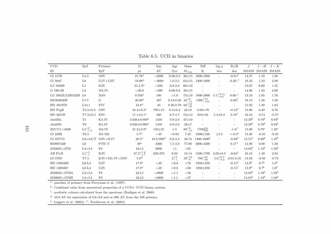
Table 6.5: UCD in binaries
UCD SpT Primary D Sep Age Mass Teff log g Fe/H J J − H J − K
ID SpT pc AU Gyr MJup K dex dex 2MASS 2MASS 2MASS
Gl 417B L4.5 G0V 21.76a ∼2000 0.08-0.3 36±15 1600-1800 - -0.01f 14.57 1.10 1.88
Gl 584C L8 G1V+G3V 18.66a ∼3600 1.0-2.5 62±15 1300-1600 - -0.20 f 16.32 1.33 2.09
GJ 1048B L1 K2V 21.2 6a ∼250 0.6-2.0 68±10 - - - 13.67 0.69 1.35
G 196-3B L2 M2.5V ∼20.0 ∼300 0.06-0.6 38±15 - - - 14.90 1.23 2.09
GJ 1001B/LHS102B L8 M4V 9.556a 180 >1.0 73±10 1900-2000 5.5+0.5−0.0
e 0.00 e 13.10 1.05 1.70
HD203030B L7.5 G 40.86a 487 0.13-0.40 24+8−11
1206+74−116
- 0.00f 18.13 1.28 1.92
HD 49197B L4±1 F5V 44.6a 43 0.26-0.79 62+12−25
- - - 15.92 1.30 1.63
HN PegB T2.5±0.5 G0V 18.4±0.3a 795±15 0.3±0.2 22±9 1130±70 - -0.12f 15.86 0.49 0.76
HD 3651B T7.5±0.5 K0V 11.1±0.1a 480 0.7-4.7 53±14 810±50 5.3±0.2 0.19f 16.16 -0.51 -0.57
εIndiBa T1 K4.5V 3.626±0.009a 1459 0.8-2.0 47±10 - - - 12.29b 0.78b 0.94b
εIndiBb T6 K4.5V 3.626±0.009a 1459 0.8-2.0 28±7 - - - 12.29b 0.78b 0.94b
2M1711+4028 L4+2−1.5 M4.5V 21.2±3.9a 135±25 1-5 69+8
−151700210
250 - -1.0f 15.00 0.79c 1.28c
Gl 229B T6.5 M1-M2 5.7a ∼45 ∼0.03 7-25 1000±100 ≤3.5 ∼-0.5e 14.20 -0.35 -0.35
Gl 337CD L8+L8/T G8V+K1V 20.5a 10.9/880d 0.6-3.4 40-74 1300-1600b - -0.29f 15.51b 0.89b 1.47b
HD89744B L0 F7IV-V 39a 2460 1.5-3.0 77-80 2000-2200 - 0.17f 14.90 0.90 1.30
2M0025+4759 L4+L4 F8 42±2 8800 <1 <65 - - - 14.84b 1.18b 1.94b
AB PicB L1+2−1
K2V 47.3+1.8−1.7 250-270 0.03 13-14 1500-1700 4.05±0.5 -0.64f 16.18 1.49 2.04
Gl 570D T7.5 K4V+M1.5V+M3V 5.9d - 2+3−1
33+18−9
780+45−30
5.0+0.3−0.2 0.01-0.10 14.82 -0.56 -0.72
HD 130948B L0-L4 G2V 17.9a ∼48 <0.8 <78 1950±250 - -0.15f 13.9b 0.7b 1.6b
HD 130948C L0-L4 G2V 17.9a ∼48 <0.8 <68 1950±250 - -0.15f 13.9b 0.7b 1.6b
2M0025+4759A L4+L4 F8 42±2 ∼8800 ∼1.1 ∼48 - - - 14.84b 1.18b 1.94b
2M0025+4759B L4+L4 F8 42±2 ∼8800 ∼1.1 ∼47 - - - 14.84b 1.18b 1.94b
a: parallax of primary from Perryman et al. (1997)b: Combined value from unresolved properties of a UCD+ UCD binary system.c: synthetic colours calculated from the spectrum (Radigan et al. 2008).d: 10.9 AU for separation of L8+L8 and at 880 AU from the MS primary.e: Leggett et al. (2002), f : Nordstrom et al. (2004).
161

UCD companions to white dwarfs
There are also a couple of known WDs with UCD companions, these have measured ages
(for the WD) and masses (for the UCDs) and are thus good benchmark systems and
included here.
The first discovered WD + UCD system, GD165AB (Becklin & Zuckerman 1988)
has been the subject of much study and is widely used as a template L dwarf. Kirkpatrick
et al. (1999a) calculated a crude age estimate for the system in a similar way to that of
GD1400, from the mass of the WD (0.56-0.65M�), taking into account the cooling age
and the main-sequence lifetime, for corresponding progenitor masses of 1.2-3M.0�. They
estimate that the age of the system is 1.2-5.5 Gyr and used the NextGen models to
calculate Teff and plot GD 165B in MK - log(age) space to compare it to model tracks for
different mass UCDs to derive a mass for GD 165B as 65-75 MJup, with a log g=5.0±0.5.
The M8.5 companion (APMPM J2354-3316C/LDS 826C) to the WD + M4 system
LHS4039/4040 (Scholz et al. 2004; Farihi, Becklin & Zuckerman 2005) is the most sim-
ilar system to 2MASSJ0030-3739/2MASSJ0030-3740 discovered in this work, having a
separation of ∼2200 AU. The age of the system was estimated at ∼1.8 Gyr by Silvestri
et al. (2001) from the M dwarf component, via it’s activity and the mass of the UCD
was calculated as ∼100MJup by Scholz et al. (2004), although they don’t state how this
was calculated. The parallax distance and J- band magnitude was used to re-evaluate
the mass of the UCD using the COND and DUSTY Lyon group models, which yield a
mass 77±3 MJup and Teff∼2260K, which places it at the stellar/substellar border. This
system, as it has a good age constraint is included here. The full list of properties of these
benchmark UCD companions to WDs are shown in Table. 6.6 and are plotted as green
stars in Fig. 6.3 - 6.5.
162

Table 6.6: UCD + WD binaries
UCD ID SpT Primary ID D Sep Age Mass Teff log g J J − H J − K
pc AU Gyr MJup K dex 2MASS 2MASS 2MASS
APMPM J2354-3316C M9.5 LHS4039/4040 ∼21 2200 ∼1.8 77±3a ∼2260a - - - -
GD 165B L4 GD 165 ∼52 ∼120 1.2-5.5 65-75 1900±100 5.0±0.5 15.6 0.90 1.51
a: Derived from the Lyon group DUSTY and COND models, b: Parallax from Van Altena et al.(1995).
163

6.2.3 Field UCDs
Although it is a difficult task to calculate the age of field UCDs, on occasion there are
indicators, such as the presence of Li in their spectra or from their kinematics (if a distance
and a radial velocity measurement are available). Several field UCDs have been identified
in this way and an age estimate calculated. The isolated field UCD DENISp-J1228.2-1547
(Delfosse et al. 1997) in which Li was observed by Tinney, Delfosse & Forveille (1997),
constraining the age to ≤1.5 Gyr. Comparison of the equivalent width measurement of
the Li feature compared to the width of this feature seen in young cluster UCDs allowed
a lower limit to be placed on the age at ≥100 Myr. Several other field UCD + UCD
binaries have also been age calibrated in this way including SDSSJ0423-0414 (Geballe
et al. 2002), where Li was measured by Burgasser et al. (2005); 2M0850 (Kirkpatrick
et al. 1999b), where Li was observed by Reid et al. (2001b) and Kelu 1 (Ruiz, Leggett &
Allard 1997). More recently Stumpf et al. (2008) has monitored Kelu1 with high resolution
VLT/NACO and HST imaging suggests that it may be a triple system, where Kelu1A is
likely to be a spectroscopic binary of type L0.5±0.5 + T7.5±1 and Kelu1B a L3pec ±1.5
dwarf. They determined a dynamical mass for the system of 177+113−55 MJup from the orbit
of the system. In addition a spectroscopic UCD + UCD binary (2MASS0320-044) in the
field was discovered by Blake et al. (2008) where the measured kinematics of the system
indicate an age >3.6 Gyr. These benchmark field UCDs are shown in Table. 6.7 and are
plotted as purple bows in Fig. 6.3 - 6.5.
164
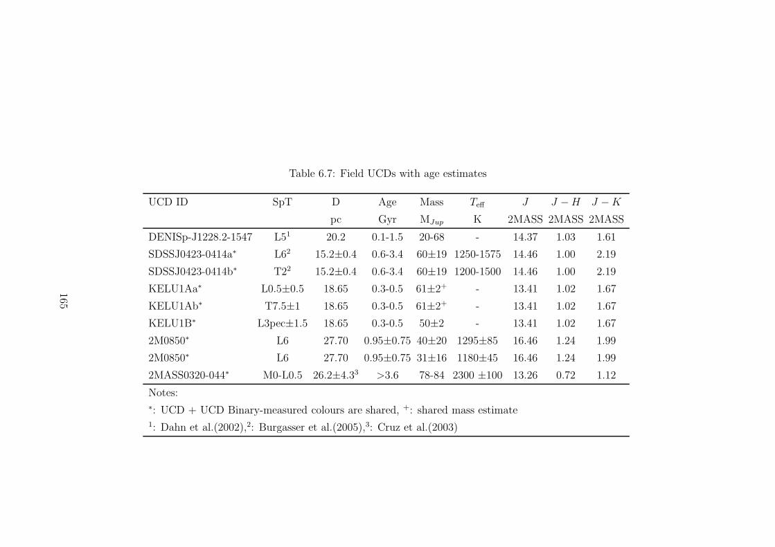
Table 6.7: Field UCDs with age estimates
UCD ID SpT D Age Mass Teff J J − H J − K
pc Gyr MJup K 2MASS 2MASS 2MASS
DENISp-J1228.2-1547 L51 20.2 0.1-1.5 20-68 - 14.37 1.03 1.61
SDSSJ0423-0414a∗ L62 15.2±0.4 0.6-3.4 60±19 1250-1575 14.46 1.00 2.19
SDSSJ0423-0414b∗ T22 15.2±0.4 0.6-3.4 60±19 1200-1500 14.46 1.00 2.19
KELU1Aa∗ L0.5±0.5 18.65 0.3-0.5 61±2+ - 13.41 1.02 1.67
KELU1Ab∗ T7.5±1 18.65 0.3-0.5 61±2+ - 13.41 1.02 1.67
KELU1B∗ L3pec±1.5 18.65 0.3-0.5 50±2 - 13.41 1.02 1.67
2M0850∗ L6 27.70 0.95±0.75 40±20 1295±85 16.46 1.24 1.99
2M0850∗ L6 27.70 0.95±0.75 31±16 1180±45 16.46 1.24 1.99
2MASS0320-044∗ M0-L0.5 26.2±4.33 >3.6 78-84 2300 ±100 13.26 0.72 1.12
Notes:∗: UCD + UCD Binary-measured colours are shared, +: shared mass estimate1: Dahn et al.(2002),2: Burgasser et al.(2005),3: Cruz et al.(2003)
165

6.3 Discussion
The benchmark UCDs identified here are plotted in Fig. 6.3 - 6.5 in mass-age, Teff -log g
and Teff -[Fe/H] space. Fig. 6.3 shows their mass-age distribution, where the distribu-
tion of objects are in reasonable agreement with the simulations of Pinfield et al. (2006)
(Fig. 6.1). Also obvious is a distance-magnitude limit, where a distance limit of 50pc
has been overplotted as an aid to indicate the limits that are currently being probed by
the benchmarks. This roughly corresponds to a detection limit of J∼19, reflecting the
sensitivity of the surveys used to detect these UCDs. Old, very low-mass objects are
not expected to be detected by these surveys as they are too faint. The distribution
also shows that the most densely populated region in mass-age space is, unsurprisingly
at younger ages, where the age can be somewhat more easily constrained, as there are
more useful age indicators (e.g. Lithium detection, activity, rotation) for youthful UCDs.
The majority of benchmarks in this region are members of clusters or moving groups,
where their metallicity is also known. It should also be noted that (omitting the candi-
date subgiant + UCD and main-sequence+UCD systems presented in this work) only a
handful have ages >2 Gyr. Thus if the candidate systems presented here are confirmed
they will make an invaluable contribution to the number of older, evolved benchmark
UCDs. These also occupy the higher mass end of the diagram. This would also allow,
if candidates confirmed, investigations of the mass-luminosity relation as a function of
time. Fig. 6.4 shows the spread in Teff and log g of the benchmarks, overplotted with the
DUSTY and COND model isochrones (red and blue lines respectively), to show where
the benchmarks sit in relation to the model parameter space. Also plotted are the bench-
marks with [Fe/H] measurements as a function of Teff in Fig. 6.5. It can be seen that the
currently confirmed benchmarks are sparsely distributed, but confirmation of UCD can-
didate companions to subgiant and main-sequence stars could provide much information
for this parameter-space. Indeed, there could be significantly more improvement via the
discovery of large additional populations of benchmarks UCDs, with a range in measured
properties, in ongoing and new large scale surveys (e.g. UKIDSS, VISTA).
166

Figure 6.3: The distribution in mass-age space for benchmark UCDs taken from the
literature and both confirmed and candidate objects (see text) presented in this work.
167

Figure 6.4: Teff against log g for benchmark UCDs taken from the literature and both
confirmed and candidate objects (see text) presented in this work. Symbols are the same
as in Fig. 6.3. Overplotted with isochrones from the Lyon group DUSTY (red) and COND
(blue) models. Solid lines are for models at 10Myr, dashed lines are for models at 100Myr,
dotted lines are 500Myr, dot-dashed lines are for 1Gyr and dot-dot-dot-dashed lines are
for 5Gyr and the long dashed lines are for 10Gyr models.
168

Figure 6.5: Teff against [Fe/H] for benchmark UCDs taken from the literature and both
confirmed and candidate objects (see text) presented in this work. Symbols are the same
as in Fig. 6.3.
169

6.3.1 The effects of gravity and metallicity on observed UCD
properties
The effects of Teff , log g and [Fe/H] on UCDs are important elements of UCD model atmo-
spheres and how they affect the colours of UCDs is still not well understood. Benchmark
objects will allow the predictions of current models to be tested and appropriately refined.
These benchmarks can be used in two ways, firstly to compare the models with observation
and thus facilitate model improvements. Secondly to look for links between observable
properties and physical characteristics and potentially calibrate changes in spectroscopic
criteria. Both are vitally important for the understanding of UCDs that may enable prop-
erties to be well constrained through observational studies (spectroscopy, photometry and
parallax). This may ultimatly lead to accurate predictions of UCD properties from their
observable (photomteric) properties alone.
In general the theory of UCD evolution is that they cool and fade over time, evolving
from L dwarfs, that have dusty atmospheres through to T dwarfs, whose atmospheres are
relatively dust-free. The two models most referenced throughout this work are from the
Lyon group, the COND (dust-free) and DUSTY models (Chabrier et al. 2000a; Baraffe
et al. 2002; Baraffe et al. 2003), which along with other models (Tucson group, Marley,
Tsuji) are effective in reproducing the overall observed characteristics of the very red,
dusty L dwarfs and those of very cool T dwarfs in the field, but struggle in particular
to explain the intermediate L/T transition phase or how the physical properties (surface
gravity or metallicity) change with age and what affect this has on their observational
characteristics. Burrows, Sudarsky & Hubeny (2006) compared the predictions for colour
from the DUSTY and COND model atmospheres. Fig. 6.6 show the predicted colours of L
and T dwarfs for different metallicity, which shows a broad variation in predicted colours,
especially across the L/T transition. Fig. 6.7 also shows a wide range in Teff -J −K colour
space, with respect to changes in gravity and metallicity predicted by models.
Knapp et al. (2004) measured accurate J-, H- and K- photometry, spectroscopy
and parallaxes for a large selection of L and T dwarfs in order to try and address this
question. They show that a large range in NIR colours and a turn over, or brightening
effect at the L/T transition, as can be seen in Fig. 6.8. The scatter in the colour sequence
is presumably caused by a range of log g and metallicity.
The cool temperatures of UCDs cause their atmospheres to be clouded by dust
of iron and silicates, which causes opacity and reddens NIR colours in L dwarfs. The
170

amount of reddening may vary with the size of the dust grains, how many there are
and their distribution in the atmosphere (Ackerman & Marley 2001; Allard et al. 2001;
Marley et al. 2002; Tsuji & Nakajima 2003). For T dwarfs dust is thought to form lower
in the atmosphere, below the photosphere, such that there is no dust opacities to affect
the emergent spectra and results in bluer NIR colours. The mechanism of this sinking or′raining-out′ of dust clouds that occurs at the L/T transition is as yet not fully understood,
as is clearly indicated by the variations in properties predicted by the models. Several
cloud models where the composition, size and rate at which condensation occurs have
been looked at to try and explain this. A scenario where dust clouds thin as Teff decreases
was proposed by Tsuji & Nakajima (2003) suggesting that the reversal in J − K colour
(as seen in Fig. 6.8) may be a function of gravity. They suggest that low gravity objects
would turn to bluer colours at brighter magnitudes compared to higher gravity objects,
indicating there could be different evolutionary tracks for varying gravities. This means
that lower mass objects would be brighter at the transition, which would occur earlier at
higher Teff and brighter MJ , whereas higher or intermediate mass objects would hit the
transition later. This would account for the observed spread in J − K colours observed
at the L/T transition.
Another theory is that of ′patchy cloud′ (Ackerman & Marley 2001; Marley et al.
2002; Burgasser et al. 2002; Folkes et al. 2007; Burgasser et al. 2008), where it is
suggested that the clouds start to break up, causing holes in the cloud deck due to
enhanced collision induced H2 absorption (CIA). Higher metallicity may also imply a
greater production of dust, as more metals are available to condense onto grains, causing
an increased opacity and reddening colours in the NIR. In general a trend in metallicity
(albeit with a large scatter) would be expected, such that older dwarfs would be expected
to have lower metallicity. This would cause a blue-ward turn in colour, suppressing the
H- and K- band flux. Indeed this may explain some of the blue L dwarfs seen, such
as 2MASSJ0532+8246, identified by Burgasser et al. (2003b) who found it to be a high
velocity, metal-poor halo object. This object has been suggested as the first substellar
sub-dwarf.
A third suggestion (see Knapp et al. 2004) is a ′sudden downpour′ model. They
suggest that at Teff∼1300K the rate of sedimentation becomes more efficient at removing
iron and silicate grains from the atmosphere, predicting that lower masses should turn
blue-ward earlier than higher masses at around T1-T4. For a T3 type they suggest a
log g∼5.4. Comparatively for the patchy cloud theory of the same spectral type, this
171

should is occur at log g≈5.0, and for the thinning cloud model log g≈4.0. Models in
general predict higher surface gravity for older UCDs, which could be tested using these
benchmarks by measuring features in their spectrum that appear to be sensitive to changes
in gravity, such as the FeH(0.869, 0.989, 1.200 & 1.600 µm), KI(1.169, 1.178, 1.243 &
1.253 µm), NaI(0.818 & 1.268) and TiO(0.705, 0.820 & 0.843 µm) features (McGovern
et al. 2004; Allers et al. 2007).
The benchmark UCDs that will be identified through the kinds of studies presented
in this work can be used to directly test these assumptions. Measuring accurate colours
and flux in the same fashion as Knapp et al. (2004) will make it possible to directly
measure, for example if the H- and K- band flux peaks in T dwarfs are really affected
by changes in gravity and metallicity, as the observations of halo UCDs (Burgasser et al.
2003b) would suggest. If gravity or metallicity are really to blame for the changes in
the strength of atomic absorption lines as suggested by the observations of McGovern
et al. (2004). Understanding the true effects of gravity and metallicity would then reveal
the mechanisms at play in the L/T transition and if/or how these factors play a part
in UCD evolution. Ultimately this would give models real predictive qualities down into
new regimes.
6.3.2 Correlations with colour and physical properties
The benchmark population that has been identified here are taken from the literature
and confirmed UCDs presented in this work (see §6.2) were used to investigate possi-
ble correlations between colours and synthetic (or modelled) physical parameters (Teff ,
log g and [Fe/H]). For the majority of the benchmarks, where all these parameters are
known, mainly broadband NIR colours are available and thus are chosen to search for
correlations amongst these. However other colours, if available may prove useful in dis-
tinguishing useful trends. For example combining NIR with optical photometry, or narrow
band colours, such as the CH4 filters in the H- band. Spectral ratios and line strengths
could also be used to investigate correlations between observable characteristics and Teff ,
log g or [Fe/H]. This would ideally be done for each spectral subclass (i.e. L0, L1...T8,
T9), however for the limited number of suitable benchmarks currently available this was
not possible and for practical reasons these were simply split into L and T. It may be
expected that this approach would be optimal given the number of available benchmarks
since dusty L dwarfs would be expected to show spectral sensitivities that will be different
172

Figure 6.6: MJ -J −K colour space showing the dependence of metallicity and gravity on
BD models from Burrows et al. (2006) for their COND (thin lines) and DUSTY (thick
lines) models. Overplotted are different metallicities for [Fe/H]=-0.5,0.0, 0.5 (blue, green
and red, respectively) and surface gravities 104.5, 105.0 and 105.5 cms−1 (the leftmost curve
from each model/metallicity set of three id for the highest gravity, and the rightmost for
the lowest) . L (filled squares) and T (filled triangles) dwarfs from Knapp et al. (2004) and
M dwarfs (open circles) from Leggett et al. (1992) are also overplotted for comparison.
Figure 6.7: Teff -J −K space predictions of the DUSTY and COND models from Burrows
et al. (2006), for a grain size of 100µm. Shown are the effects of changes in [Fe/H] of 0.5
(red), 0.0 (green) and -0.5 (blue) and log g of 4.5 (dashed lines), 5.0 (solid lines) and 5.5
(dot-dashed lines).
173

Figure 6.8: Left: MJ as a function of spectral type and Right: MJ as a function of
J − K colour for L and T dwarfs from Knapp et al. (2004). Objects circled are known
binaries and error bars are shown where the type is uncertain by more than one subclass.
Overplotted are the cloud-free models from Marley et al. (2002) for varying values of log g.
to those of the relatively dust-free atmospheres of T dwarfs. In the following sections the
steps undertaken to search for property related correlations with broadband colour are
explained.
Correlations with colour and Teff
The benchmark L’s and T’s were firstly plotted as a function of Teff against J −H, H−K
and J − K colour. A least squares fit was made to provide a first approximation fit. For
this approximation the L dwarf benchmarks show a linear trend if 1207B is removed from
the fit data. 1207B likely suffers from gray dust extinction in the NIR, which causes it to
be under luminous (Mamajek 2005). This means that the constraints on log g for 1207B
are poor, with an estimate from the available models giving log g over a large range of
4.5-5.5. On reflection this object does not make a good benchmark for assessing colour-
property correlations, despite 1207B being a promising object, where an insight into the
potential trends for planetary mass UCDs could have been indicated. This object is
highlighted in Fig. 6.9 and the fit to the T dwarfs are shown in Fig. 6.10, where again a
linear trend provides the best fit.
174

Figure 6.9: Teff -colour plot of benchmark L dwarfs with NIR J − H, H − K and J − K
colours. Overplotted as a dotted line is a least squares fit to the data. Also overplotted
is 1207B (as a square), see text.
Figure 6.10: Teff -colour plot of benchmark T dwarfs from the literature search with NIR
J − H, H − K and J − K colours. Overplotted as a dotted line is a least squares fit to
the data. Also highlighted is Gl 229B as a square as a potential log g and [Fe/H] outlier,
with normal T dwarf colours (see text).
175

Correlations with colour and log g and [Fe/H]
The first approximation fits were used to create a Teff corrected colour, and any trends
with log g or [Fe/H] were looked for. For the T dwarfs only four benchmarks had known
Teff , log g and [Fe/H], one of which is Gl 229B, an unusually low-gravity, metal poor T
dwarf (based on the observations and analysis of Leggett et al. 2002a). Models predict
that log g should increase as an object cools and contracts, with which metallicity should
decrease as more heavier elements are created over time. If colours are dependent on
these properties then it may be possible that these contrasting effects could cancel out
any correlation with colour. This may be the underlying reason for the apparent normal
T dwarf colours that Gl 229B exhibits (highlighted as a square symbol in Fig. 6.10).
There are several more L dwarf benchmarks than T’s, however the scatter in colours
implies no obvious trend. Most of the objects lie between log g = 4.5 and 5.0, with two
objects at log g = 5.5, GD 165B, a companion to a WD and HD12005C, a companion
to a main-sequence star (confirmed in this work). The low gravity end is occupied by
ABpicB, a similarly low-gravity metal poor UCD as Gl 229B and the binary 1207AB,
where 1207B has large uncertainties (indicated by error bars in Fig. 6.11). There is no
obvious trend here, but if the uncertainties on 1207B were smaller then it may indicate a
red-ward trend in NIR colour at low log g.
For metallicity the limited number of objects, including Gl 229B, means that a
trend could not be fully analysed for the T dwarfs. For the L dwarfs, although the sample
numbers with [Fe/H] are larger, the spread in colour is quite large with the majority of
objects occupying mainly two metallicity bins; the Hyades L dwarf objects at [Fe/H]∼0.14
and main-sequence companions and Pleiades UCDs with solar metallicity. The spread in
colours is also quite sizable here. Therefore, although there may be some relation between
broadband colour and metallicity, it would not be possible to see it because neither the
sample size nor the range of properties within the population of benchmark L and T
dwarfs are available.
176

Figure 6.11: Colour against log g, where the colour-Teff trend (see Fig. 6.9) has been
subtracted from the colour, for benchmark L dwarfs with NIR J −H, H −K and J −K
colours. Overplotted as a dotted line is a least squares fit to the data. Also overplotted
is the outlier 1207B (as a square) with its error bars (see text).
Figure 6.12: Colour against log g, where the colour-Teff trend (see Fig. 6.10) has been
subtracted from the colour, for benchmark T dwarfs with NIR J −H, H −K and J −K
colours. Overplotted as a dotted line is a least squares fit to the data. Also highlighted
is Gl 229B as a square, as a potential log g and [Fe/H] outlier (see text).
177

Figure 6.13: Colour against [Fe/H], where the colour-Teff trend (see Fig. 6.9) has been
subtracted from the colour, for benchmark L dwarfs with NIR J −H, H −K and J −K
colours. Overplotted as a dotted line is a least squares fit to the data. Also overplotted
are the outliers 1207B (as a square), see text.
Figure 6.14: Colour against [Fe/H], where the colour-Teff trend (see Fig. 6.10) has been
subtracted from the colour, for benchmark T dwarfs with NIR J −H, H −K and J −K
colours. Overplotted as a dotted line is a least squares fit to the data. Also highlighted
is Gl 229B as a square, as a potential log g and [Fe/H] outlier (see text).
178

Sensitivity of colours to Teff
If there had been obvious trends to colour and log g or [Fe/H] then it would be possible to
produce improved colour-Teff fits by removing the trends in colour derived for the log g and
[Fe/H]. This would be expected to reduce the scatter in the colour-Teff plot. This method
is illustrated here, using the essentially zero trend findings for log g and [Fe/H], even
though the scatter has not changed. The ′improved′ colour-Teff fit is shown in Fig. 6.15
for the L dwarfs. There appears a fairly linear trend with Teff and colours (overplotted as
a dotted line on Fig. 6.15) and in general the scatter is smallest in H −K for both the L
and T dwarfs. The range over which the properties are best fit was determined from the
level of scatter and the distribution of data points along the fit. For the T dwarfs, objects
are fairly evenly distributed in Teff space. However for L dwarfs there are no objects
between 2100-2500K and it is possible the trend in that region may not be linear.
A more comprehensive investigation of benchmark sensitivity to physical properties
would investigate a much greater range of observable criteria (other than broadband
photometry). However, this is limited by the available benchmarks and measurements,
and thus it has only been possible to identify trends between Teff and the three NIR
colours considered.
These trends were used to calculate a sensitivity index in the applicable Teff ranges,
as the rate of change of colour with Teff . The equation of the fit is a first order, least
squares fit of the form Colour = a + b(Teff ), where a and b are the coefficients of the fit
and the corresponding sensitivity is shown in Table. 6.8 and 6.9. The larger the sensitivity
index, the more sensitive the colour is to changes in Teff . On inspection of the sensitivity
of NIR broadband colours with Teff , the benchmarks would indicate that the colours are,
in general not strongly sensitive to changes in Teff , but that of all the colours J −K might
be slightly more sensitive than J −H and H−K colours. From these correlations the Teff
of a UCD can also be calculated, such that for a UCD with solar metallicity, log g∼5.0,
over the range 750≤Teff ≤1400 (for T dwarfs) and 1600≤Teff≤2100 (L dwarfs), Teff can
be approximated via the following relations.
L dwarf colour-Teff relations:
Teff=2830.74-983.95(J − H)
Teff=2790.22-1438.28(H − K)
Teff=2907.41-630.03(J − K)
179

Table 6.8: Parameters of fitting equations for colours of T dwarfs.
Colour Property a b Range Sensitivitya
J − H Teff -2.671 0.0026 750-1400K 0.0026
H − K Teff -1.075 0.0011 750-1400K 0.0112
J − K Teff -3.658 0.0039 750-1400K 0.0375
Notes: The relation equation is: colour=a+b*Teff .
a Sensitivity is the rate of change of colour with Teff .
Table 6.9: Parameters of fitting equations for colours of L dwarfs.
Colour Property a b Range Sensitivitya
J − H Teff 1.879 -0.00049 1600-2100K 0.00050
H − K Teff 1.303 -0.00036 1600-2100K 0.00035
J − K Teff 3.233 -0.00086 1600-2100K 0.00085
Notes: The relation equation is: colour=a+b*Teff .
a Sensitivity is the rate of change of colour with Teff .
T dwarf colour-Teff relations:
Teff=1023.48+353.30(J − H)
Teff=947.38+845.58(H − K)
Teff=995.09+252.49(J − K)
Although no strong correlation between broadband colour and log g or [Fe/H] are
seen, and only a weak relation to Teff has been found in this study, there are indications
(i.e. from the remaining scatter in colours and the properties of some outlying objects),
these analytical techniques hold promise for the future. With more benchmark UCDs and
a greater spread in properties over a range of spectral types it may be possible to provide
a way of robustly measuring UCD properties from their observable characteristics. Good
relations with colour may also allow reliable mass functions to be calculated with a only
a limited amount of spectroscopic follow-up.
180

Figure 6.15: Improved Teff against colour plot, where the effects of log g and [Fe/H] (from
Fig. 6.11 and 6.13) have been removed for the benchmark L dwarfs with NIR J − H,
H −K and J −K colours. Overplotted as a dotted line is a least squares fit to the data.
181

6.4 Future Work
The work in this thesis has presented the discovery of three UCD companions to main-
sequence and WD stars, two of which are benchmark systems with constrained ages,
along with a large number of candidate UCD + WD, UCD + main-sequence and UCD
+ subgiant binary systems. The next logical progression would be to follow-up these
candidates with a combination of proper motion, parallax and spectral observations. Once
confirmed, high S/N or high resolution spectroscopy could be employed to accurately
measure such gravity sensitive features as previously mentioned. They could then be
used to calibrate properties observationally and place constraints on evolutionary models.
Correlations with colour and properties could also be explored, enabling a way to infer
the properties of a UCD based on its observable colours.
The large number of benchmarks needed for this task could be found by expanding
this work. In the immediate/near future this includes future data releases of large NIR
surveys such as UKIDSS and the VISTA hemisphere survey, which is planned to reach
a further ∼2 magnitudes fainter than UKIDSS (K ∼20), over a large portion of the
southern hemisphere and will be able to probe deeper and fainter than previously capable
and should reveal hundreds of new UCDs and many in new lower temperature regimes,
where the question of a BD minimum mass can also start to be addressed.
In addition WISE will be able to follow-up benchmark UCDs by measuring their
mid IR flux. This coupled with a parallax distance will enable a direct measurement
of luminosity, where combined with age information can give a radius estimate from
structure models and will allow Teff , mass and log g to be calculated. Another natural
expansion of this work would be to extend the subgiant pilot survey, where an accurate
measurement of metallicity (if not known) could be calculated from follow-up echelle
spectra. The WDs however will not yield this information, but obtaining high resolution
spectra will allow accurate determinations of the cooling age to be calculated, placing very
accurate constraints on the age of WD + UCD systems. The UCDs discovered through
these methods will also allow constraints to be placed on the binary fraction, birth rate
and the mass function for ultracool objects. These factors are vitally important for the
understanding of the substellar population in the galaxy.
182

References
Ackerman A. S., Marley M. S., 2001, ApJ, 556, 872Allard F., Hauschildt P. H., Alexander D. R., Tamanai A., Schweitzer A., 2001, ApJ, 556,
357Allen P. R., Koerner D. W., Reid I. N., Trilling D. E., 2005, ApJ, 625, 385Allers K. N. et al., 2007, ApJ, 657, 511Althaus L. G., Garcıa-Berro E., Corsico A. H., Miller Bertolami M. M., Romero A. D.,
2009, ApJL, 693, L23Andersen M., Meyer M. R., Greissl J., Aversa A., 2008, ApJL, 683, L183Balega I., Balega Y. Y., Maksimov A. F., Pluzhnik E. A., Schertl D., Shkhagosheva Z. U.,
Weigelt G., 2004, A&A, 422, 627Baraffe I., Chabrier G., Allard F., Hauschildt P. H., 1998, A&A, 337, 403Baraffe I., Chabrier G., Allard F., Hauschildt P. H., 2002, A&A, 382, 563Baraffe I., Chabrier G., Barman T. S., Allard F., Hauschildt P. H., 2003, A&A, 402, 701Barry D. C., 1988, ApJ, 334, 436Basri G., 1998, in Rebolo R., Martin E. L., Zapatero Osorio M. R., eds, Brown Dwarfs
and Extrasolar Planets. p. 394Bate M. R., Bonnell I. A., Bromm V., 2003, MNRAS, 339, 577Bate M. R., 1998, ApJL, 508, L95Bate M. R., 2005, MNRAS, 363, 363Becklin E. E., Zuckerman B., 1988, Nature, 336, 656Benvenuto O. G., Althaus L. G., 1999, MNRAS, 303, 30Bergeron P., Gianninas A., Boudreault S., 2007, in Napiwotzki R., Burleigh M. R., eds,
15th European Workshop on White Dwarfs. p. 29Bessell M. S., 1986, PASP, 98, 1303Bihain G., Rebolo R., Bejar V. J. S., Caballero J. A., Bailer-Jones C. A. L., Mundt R.,
Acosta-Pulido J. A., Manchado Torres A., 2006, A&A, 458, 805Blake C. H., Charbonneau D., White R. J., Torres G., Marley M. S., Saumon D., 2008,
ApJL, 678, L125Bochanski J. J., West A. A., Hawley S. L., Covey K. R., 2007, AJ, 133, 531Boehm-Vitense E., 1992, Introduction to stellar astrophysics. Vol. 3 - Stellar structure
and evolution. Cambridge, England and New York, Cambridge University Press,1992, 300 p.
Bonfils X., Delfosse X., Udry S., Santos N. C., Forveille T., Segransan D., 2005, A&A,442, 635
Bouvier J., Stauffer J. R., Martin E. L., Barrado y Navascues D., Wallace B., Be-jar V. J. S., 1998, A&A, 336, 490
Bouvier J. et al., 2008, A&A, 481, 661Briceno C., Luhman K. L., Hartmann L., Stauffer J. R., Kirkpatrick J. D., 2002, ApJ,
580, 317Burgasser A. J., Burrows A., Kirkpatrick J. D., 2006, ApJ, 639, 1095Burgasser A. J. et al., 2000, ApJL, 531, L57Burgasser A. J. et al., 2002, ApJ, 564, 421Burgasser A. J., Geballe T. R., Golimowski D. A., Leggett S. K., Kirkpatrick J. D.,
183

Knapp G. R., Fan X., 2003, in Martın E., ed, Brown Dwarfs. p. 377Burgasser A. J. et al., 2003, ApJ, 592, 1186Burgasser A. J., McElwain M. W., Kirkpatrick J. D., Cruz K. L., Tinney C. G., Reid I. N.,
2004, AJ, 127, 2856Burgasser A. J., Reid I. N., Leggett S. K., Kirkpatrick J. D., Liebert J., Burrows A., 2005,
ApJL, 634, L177Burgasser A. J., Geballe T. R., Leggett S. K., Kirkpatrick J. D., Golimowski D. A., 2006,
ApJ, 637, 1067Burgasser A. J., Looper D. L., Kirkpatrick J. D., Cruz K. L., Swift B. J., 2008, ApJ, 674,
451Burgasser A. J., Kirkpatrick J. D., Lowrance P. J., 2005, AJ, 129, 2849Burgasser A. J., 2004, ApJS, 155, 191Burgasser A. J., 2007, ApJ, 658, 617Burleigh M. R., Clarke F. J., Hodgkin S. T., 2002, MNRAS, 331, L41Burleigh M. R., Hogan E., Dobbie P. D., Napiwotzki R., Maxted P. F. L., 2006, MNRAS,
373, L55Burleigh M. R. et al., 2006, MNRAS, 373, 1416Burningham B. et al., 2008, MNRAS, 391, 320Burrows A., Hubbard W. B., Lunine J. I., Marley M., Guillot T., Saumon D., Freed-
man R. S., 1997a, in Soderblom D., ed, Planets Beyond the Solar System and theNext Generation of Space Missions. p. 9
Burrows A. et al., 1997, ApJ, 491, 856Burrows A., Hubbard W. B., Lunine J. I., Liebert J., 2001, Reviews of Modern Physics,
73, 719Burrows A., Sudarsky D., Hubeny I., 2006, ApJ, 640, 1063Burrows A., Sudarsky D., Lunine J. I., 2003, ApJ, 596, 587Burstein D., Heiles C., 1982, AJ, 87, 1165Carpenter J. M., 2001, AJ, 121, 2851Casali M. et al., 2007, A&A, 467, 777Casewell S. L., Dobbie P. D., Hodgkin S. T., Moraux E., Jameson R. F., Hambly N. C.,
Irwin J., Lodieu N., 2007, MNRAS, 378, 1131Catalan S., Isern J., Garcıa-Berro E., Ribas I., Allende Prieto C., Bonanos A. Z., 2008,
A&A, 477, 213Cayrel de Strobel G., Soubiran C., Friel E. D., Ralite N., Francois P., 1997, A&AS, 124,
299Chabrier G., Baraffe I., Plez B., 1996, ApJL, 459, L91+Chabrier G., Baraffe I., Allard F., Hauschildt P., 2000, ApJ, 542, 464Chabrier G., Brassard P., Fontaine G., Saumon D., 2000, ApJ, 543, 216Chabrier G., Brassard P., Fontaine G., Saumon D., 2000, ApJ, 543, 216Chabrier G., 2003, PASP, 115, 763Chandrasekhar S., 1931, ApJ, 74, 81Chappelle R. J., Pinfield D. J., Steele I. A., Dobbie P. D., Magazzu A., 2005, MNRAS,
361, 1323Chauvin G. et al., 2005, A&A, 438, L29Chiu K., Fan X., Leggett S. K., Golimowski D. A., Zheng W., Geballe T. R., Schnei-
184

der D. P., Brinkmann J., 2006, AJ, 131, 2722Claver C. F., Liebert J., Bergeron P., Koester D., 2001, ApJ, 563, 987Comeron F., Reipurth B., Henry A., Fernandez M., 2004, A&A, 417, 583Cossburn M. R., Hodgkin S. T., Jameson R. F., Pinfield D. J., 1997, MNRAS, 288, L23Cruz K. L., Reid I. N., Liebert J., Kirkpatrick J. D., Lowrance P. J., 2003, AJ, 126, 2421Cruz K. L. et al., 2007, AJ, 133, 439Cushing M. C., Rayner J. T., Vacca W. D., 2005, ApJ, 623, 1115Dahn C. C. et al., 2002, AJ, 124, 1170Day-Jones A. C. et al., 2008, MNRAS, 388, 838De Simone R., Wu X., Tremaine S., 2004, MNRAS, 350, 627Deacon N. R., Hambl N. C., 2004, A&A, 416, 125Delfosse X. et al., 1997, A&A, 327, L25Delorme P. et al., 2008, A&A, 482, 961Dobbie P. D., Pinfield D. J., Napiwotzki R., Hambly N. C., Burleigh M. R., Barstow Jame-
son R. F., Hubeny I., 2004, MNRAS, 355, L39Dobbie P. D., Burleigh M. R., Levan A. J., Barstow M. A., Napiwotzki R., Holberg J. B.,
Hubeny I., Howell S. B., 2005, MNRAS, 357, 1049Dobbie P. D. et al., 2006, MNRAS, 369, 383Dufour P., Fontaine G., Liebert J., Schmidt G. D., Behara N., 2008, ApJ, 683, 978Dye S. et al., 2006, MNRAS, 372, 1227Edvardsson B., Andersen J., Gustafsson B., Lambert D. L., Nissen P. E., Tomkin J., 1993,
A&A, 275, 101Eisenstein D. J. et al., 2006, ApJS, 167, 40Engelbrecht A., Koester D., 2007, in Napiwotzki R., Burleigh M. R., eds, 15th European
Workshop on White Dwarfs. p. 289EROS Collaboration et al., 1999, A&A, 351, L5Fan X. et al., 2001, AJ, 121, 54Farihi J., Christopher M., 2004, AJ, 128, 1868Farihi J., Becklin E. E., Zuckerman B., 2005, ApJS, 161, 394Farihi J., Becklin E. E., Zuckerman B., 2008, ApJ, 681, 1470Farihi J., Burleigh M. R., Hoard D. W., 2008, ApJ, 674, 421Farihi J., Hoard D. W., Wachter S., 2006, ApJ, 646, 480Farihi J., Zuckerman B., Becklin E. E., 2008, ApJ, 674, 431Feltzing S., Gustafsson B., 1998, A&AS, 129, 237Feltzing S., Holmberg J., Hurley J. R., 2001, VizieR Online Data Catalog, 337, 70911Ferrario L., Wickramasinghe D., Liebert J., Williams K. A., 2005, MNRAS, 361, 1131Finley D. S., Koester D., Basri G., 1997, ApJ, 488, 375Fleming T. A., Schmitt J. H. M. M., Giampapa M. S., 1995, ApJ, 450, 401Folkes S. L., Pinfield D. J., Kendall T. R., Jones H. R. A., 2007, MNRAS, 378, 901Funayama H., Itoh Y., Oasa Y., Toyota E., Mukai T., 2008, in Santos N. C., Pasquini L.,
Correia A. C. M., Romaniello M., eds, Precision Spectroscopy in Astrophysics.p. 285
Geballe T. R., Saumon D., Leggett S. K., Knapp G. R., Marley M. S., Lodders K., 2001,ApJ, 556, 373
Geballe T. R. et al., 2002, ApJ, 564, 466
185

Geballe T. R., Knapp G. R., Leggett S. K., Fan X., Golimowski D. A., 2003, in Brown A.,Harper G. M., Ayres T. R., eds, The Future of Cool-Star Astrophysics: 12th Cam-bridge Workshop on Cool Stars, Stellar Systems, and the Sun (2001 July 30 - August3), eds. A. Brown, G.M. Harper, and T.R. Ayres, (University of Colorado), 2003, p.670-675. p. 670
Geißler K. et al., 2007, A&A, 461, 665Girardi L., Bressan A., Bertelli G., Chiosi C., 2000, VizieR Online Data Catalog, 414,
10371Gizis J. E., Bharat R., 2004, ApJL, 608, L113Gizis J. E., Kirkpatrick J. D., Burgasser A., Reid I. N., Monet D. G., Liebert J., Wil-
son J. C., 2001, ApJL, 551, L163Gizis J. E., Kirkpatrick J. D., Wilson J. C., 2001, AJ, 121, 2185Gizis J. E., Reid I. N., Hawley S. L., 2002, AJ, 123, 3356Golimowski D. A. et al., 2004, AJ, 127, 3516Goodwin S. P., Whitworth A., 2007, A&A, 466, 943Green E. M., Demarque P., King C. R., 1987, The revised Yale isochrones and luminosity
functions. The revised Yale isochrones and luminosity functions, New Haven: YaleObservatory, 1987
Grether D., Lineweaver C. H., 2006, ApJ, 640, 1051Guieu S., Dougados C., Monin J.-L., Magnier E., Martın E. L., 2006, A&A, 446, 485Hambly N. C., Digby A. P., Oppenheimer B. R., 2005, in Koester D., Moehler S., eds,
14th European Workshop on White Dwarfs. p. 113Hambly N. C., Hodgkin S. T., Cossburn M. R., Jameson R. F., 1999, MNRAS, 303, 835Hambly N. C. et al., 2008, MNRAS, 384, 637Hauck B., Mermilliod M., 1985, A&AS, 60, 61Hauck B., Mermilliod M., 1998, A&AS, 129, 431Hawley S. L. et al., 2002, AJ, 123, 3409Hempelmann A., Schmitt J. H. M. M., Schultz M., Ruediger G., Stepien K., 1995, A&A,
294, 515Hewett P. C., Warren S. J., Leggett S. K., Hodgkin S. T., 2006, MNRAS, 367, 454Hillenbrand L. A., 1997, AJ, 113, 1733Hogan E., Jameson R. F., Casewell S. L., Osbourne S. L., Hambly N. C., 2008, MNRAS,
388, 495Howell S. B., Nelson L. A., Rappaport S., 2001, ApJ, 550, 897Hubeny I., Lanz T., 1995, ApJ, 439, 875Hurley J. R., Pols O. R., Tout C. A., 2000, MNRAS, 315, 543Ibukiyama A., Arimoto N., 2002, A&A, 394, 927Ireland M. J., Kraus A., Martinache F., Lloyd J. P., Tuthill P. G., 2008, ApJ, 678, 463Jameson R. F., Casewell S. L., Bannister N. P., Lodieu N., Keresztes K., Dobbie P. D.,
Hodgkin S. T., 2008, MNRAS, 384, 1399Jeans J. H., 1924, MNRAS, 85, 2Jenkins J. S., Jones H. R. A., Pavlenko Y., Pinfield D. J., Barnes J. R., Lyubchik Y.,
2008, A&A, 485, 571Jones H. R. A., Pavlenko Y., Viti S., Barber R. J., Yakovina L. A., Pinfield D., Ten-
nyson J., 2005, MNRAS, 358, 105
186

Just A., 2003, Ap&SS, 284, 727Kalirai J. S., Hansen B. M. S., Kelson D. D., Reitzel D. B., Rich R. M., Richer H. B.,
2008, ApJ, 676, 594Kilic M. et al., 2006, AJ, 131, 582Kilkenny D., Heber U., Drilling J. S., 1988, South African Astronomical Observatory
Circular, 12, 1Kirkpatrick J. D., Allard F., Bida T., Zuckerman B., Becklin E. E., Chabrier G., Baraffe I.,
1999, ApJ, 519, 834Kirkpatrick J. D. et al., 1999, ApJ, 519, 802Kirkpatrick J. D. et al., 2000, AJ, 120, 447Kirkpatrick J. D., Dahn C. C., Monet D. G., Reid I. N., Gizis J. E., Liebert J., Bur-
gasser A. J., 2001, AJ, 121, 3235Kleinman S. J. et al., 2004, ApJ, 607, 426Knapp G. R. et al., 2004, AJ, 127, 3553Knox R. A., Hawkins M. R. S., Hambly N. C., 1999, MNRAS, 306, 736Kroupa P., 2001, MNRAS, 322, 231Kumar S. S., 1963, ApJ, 137, 1121Lachaume R., Dominik C., Lanz T., Habing H. J., 1999, A&A, 348, 897Latham D. W., Stefanik R. P., Torres G., Davis R. J., Mazeh T., Carney B. W.,
Laird J. B., Morse J. A., 2002, AJ, 124, 1144Lawrence A. et al., 2007, MNRAS, 379, 1599Leggett S. K., Toomey D. W., Geballe T. R., Brown R. H., 1999, ApJL, 517, L139Leggett S. K. et al., 2002, ApJ, 564, 452Leggett S. K., Hauschildt P. H., Allard F., Geballe T. R., Baron E., 2002, MNRAS, 332,
78Leggett S. K., 1992, ApJS, 82, 351Levine J. L., Steinhauer A., Elston R. J., Lada E. A., 2006, ApJ, 646, 1215Liebert J., Bergeron P., Holberg J. B., 2005, ApJS, 156, 47Littlefair S. P., Dhillon V. S., Marsh T. R., Gansicke B. T., Southworth J., Watson C. A.,
2006, Science, 314, 1578Liu M. C., Dupuy T. J., Ireland M. J., 2008, arXivLiu M. C., Leggett S. K., Chiu K., 2007, ApJ, 660, 1507Lodieu N., Dobbie P. D., Deacon N. R., Hodgkin S. T., Hambly N. C., Jameson R. F.,
2007, MNRAS, 380, 712Lodieu N. et al., 2007, MNRAS, 379, 1423Lodieu N., Hambly N. C., Jameson R. F., Hodgkin S. T., 2008, MNRAS, 383, 1385Lodieu N., Hambly N. C., Jameson R. F., 2006, MNRAS, 373, 95Lucas P. W., Weights D. J., Roche P. F., Riddick F. C., 2006, MNRAS, 373, L60Luhman K. L., Rieke G. H., 1999, ApJ, 525, 440Luhman K. L., Rieke G. H., Young E. T., Cotera A. S., Chen H., Rieke M. J., Schneider G.,
Thompson R. I., 2000, ApJ, 540, 1016Luhman K. L., Briceno C., Stauffer J. R., Hartmann L., Barrado y Navascues D., Cald-
well N., 2003, ApJ, 590, 348Luhman K. L., Stauffer J. R., Muench A. A., Rieke G. H., Lada E. A., Bouvier J.,
Lada C. J., 2003, ApJ, 593, 1093
187

Luhman K. L. et al., 2007, ApJ, 654, 570Luhman K. L., 2004, ApJ, 602, 816Luhman K. L., 2007, ApJS, 173, 104Magazzu A., Rebolo R., Zapatero Osorio M. R., Martin E. L., Hodgkin S. T., 1998, ApJL,
497, L47+Mamajek E. E., 2005, ApJ, 634, 1385Marley M. S., Seager S., Saumon D., Lodders K., Ackerman A. S., Freedman R. S., Fan X.,
2002, ApJ, 568, 335Marsakov V. A., Shevelev Y. G., 1995, Bulletin d’Information du Centre de Donnees
Stellaires, 47, 13Martın E. L., Basri G., Zapatero-Osorio M. R., Rebolo R., Lopez R. J. G., 1998, ApJL,
507, L41Martın E. L., Delfosse X., Basri G., Goldman B., Forveille T., Zapatero Osorio M. R.,
1999, AJ, 118, 2466Martın E. L., Rebolo R., Zapatero-Osorio M. R., 1996, ApJ, 469, 706Maxted P. F. L., Napiwotzki R., Dobbie P. D., Burleigh M. R., 2006, Nature, 442, 543McCaughrean M. J., Close L. M., Scholz R. D., Lenzen R., Biller B., Brandner W.,
Hartung M., Lodieu N., 2004, A&A, 413, 1029McCook G. P., Sion E. M., 1999, ApJS, 121, 1McGovern M. R., Kirkpatrick J. D., McLean I. S., Burgasser A. J., Prato L.,
Lowrance P. J., 2004, ApJ, 600, 1020McLean I. S. et al., 2000, ApJL, 533, L45McLean I. S., McGovern M. R., Burgasser A. J., Kirkpatrick J. D., Prato L., Kim S. S.,
2003, ApJ, 596, 561Metchev S. A., Hillenbrand L. A., 2004, ApJ, 617, 1330Metchev S. A., Hillenbrand L. A., 2006, ApJ, 651, 1166Miller G. E., Scalo J. M., 1979, ApJS, 41, 513Mohanty S., Jayawardhana R., Huelamo N., Mamajek E., 2007, ApJ, 657, 1064Mohanty S., Jayawardhana R., Basri G., 2005, ApJ, 626, 498Monet D. G., Dahn C. C., Vrba F. J., Harris H. C., Pier J. R., Luginbuhl C. B.,
Ables H. D., 1992, AJ, 103, 638Monet D. G. et al., 2003, AJ, 125, 984Monteiro H., Jao W.-C., Henry T., Subasavage J., Beaulieu T., 2006, ApJ, 638, 446Moraux E., Bouvier J., Stauffer J. R., Cuillandre J.-C., 2003, A&A, 400, 891Muench A. A., Lada E. A., Lada C. J., Alves J., 2002, ApJ, 573, 366Muench A. A. et al., 2003, AJ, 125, 2029Mugrauer M., Seifahrt A., Neuhauser R., Mazeh T., 2006, MNRAS, 373, L31Mullally F., Kilic M., Reach W. T., Kuchner M. J., von Hippel T., Burrows A.,
Winget D. E., 2007, ApJS, 171, 206Nakajima T., Oppenheimer B. R., Kulkarni S. R., Golimowski D. A., Matthews K.,
Durrance S. T., 1995, Nature, 378, 463Napiwotzki R. et al., 2001, Astronomische Nachrichten, 322, 411Napiwotzki R., Green P. J., Saffer R. A., 1999, ApJ, 517, 399Nordstrom B. et al., 2004, VizieR Online Data Catalog, 5117, 0Padoan P., Nordlund A., 2002, ApJ, 576, 870
188

Panei J. A., Althaus L. G., Benvenuto O. G., 2000, A&A, 353, 970Perryman M. A. C. et al., 1997, A&A, 323, L49Perryman M. A. C. et al., 1998, A&A, 331, 81Pinfield D. J., Dobbie P. D., Jameson R. F., Steele I. A., Jones H. R. A., Katsiyannis A. C.,
2003, MNRAS, 342, 1241Pinfield D. J., Jones H. R. A., Lucas P. W., Kendall T. R., Folkes S. L., Day-Jones A. C.,
Chappelle R. J., Steele I. A., 2006, MNRAS, 368, 1281Pinfield D. J. et al., 2008, arXiv, 806Pollack J. B., Hubickyj O., Bodenheimer P., Lissauer J. J., Podolak M., Greenzweig Y.,
1996, Icarus, 124, 62Potter D., Martın E. L., Cushing M. C., Baudoz P., Brandner W., Guyon O.,
Neuhauser R., 2002, ApJL, 567, L133Pravdo S. H., Shaklan S. B., Lloyd J., 2005, ApJ, 630, 528Prialnik D., 2000, An Introduction to the Theory of Stellar Structure and Evolution. An
Introduction to the Theory of Stellar Structure and Evolution, by D. Prialnik. ISBN052165937X, Cambridge University Press, 2000.
Radigan J., Lafreniere D., Jayawardhana R., Doyon R., 2008, arXivRebolo R., Zapatero Osorio M. R., Madruga S., Bejar V. J. S., Arribas S., Licandro J.,
1998, Science, 282, 1309Rebolo R., Zapatero-Osorio M. R., Martin E. L., 1995, Nature, 377, 129Reid I. N. et al., 1999, ApJ, 521, 613Reid I. N., Burgasser A. J., Cruz K. L., Kirkpatrick J. D., Gizis J. E., 2001, AJ, 121, 1710Reid I. N., Gizis J. E., Kirkpatrick J. D., Koerner D. W., 2001, AJ, 121, 489Reid I. N., Lewitus E., Allen P. R., Cruz K. L., Burgasser A. J., 2006, AJ, 132, 891Reipurth B., Clarke C., 2001, AJ, 122, 432Ribas I., 2003, A&A, 400, 297Rocha-Pinto H. J., Scalo J., Maciel W. J., Flynn C., 2000, ApJL, 531, L115Roxburgh I. W., 1989, A&A, 211, 361Ruiz M. T., Leggett S. K., Allard F., 1997, ApJL, 491, L107+Salpeter E. E., 1955, ApJ, 121, 161Santos Jr. J. F. C., Piatti A. E., 2004, A&A, 428, 79Saumon D., Marley M. S., Lodders K., Freedman R. S., 2003, in Martın E., ed, Brown
Dwarfs. p. 345Saumon D. et al., 2007, ApJ, 656, 1136Scalo J. M., 1986, in de Loore C. W. H., Willis A. J., Laskarides P., eds, Luminous Stars
and Associations in Galaxies. p. 451Scholz A., Jayawardhana R., 2006, ApJ, 638, 1056Scholz R.-D., McCaughrean M. J., Lodieu N., Kuhlbrodt B., 2003, A&A, 398, L29Scholz R.-D., Lodieu N., Ibata R., Bienayme O., Irwin M., McCaughrean M. J.,
Schwope A., 2004, MNRAS, 347, 685Scholz A., Jayawardhana R., Brandeker A., 2005, ApJL, 629, L41Schroder K.-P., Pauli E.-M., Napiwotzki R., 2004, MNRAS, 354, 727Schuster W. J., Nissen P. E., 1989, A&A, 222, 69Schwartz M. J., Becklin E. E., 2005, AJ, 130, 2352Silvestri N. M., Oswalt T. D., Wood M. A., Smith J. A., Reid I. N., Sion E. M., 2001,
189

AJ, 121, 503Sion E. M., Greenstein J. L., Landstreet J. D., Liebert J., Shipman H. L., Wegner G. A.,
1983, ApJ, 269, 253Skrutskie M. F. et al., 2006, AJ, 131, 1163Slesnick C. L., Hillenbrand L. A., Carpenter J. M., 2004, ApJ, 610, 1045Stark M. A., Wade R. A., 2003, AJ, 126, 1455Steele P. R., Burleigh M. R., Dobbie P. D., Barstow M. A., 2007, MNRAS, 382, 1804Stumpf M. B., Brandner W., Henning T., Bouy H., Koehler R., Hormuth F., Joergens V.,
Kasper M., 2008, arXivTej A., Sahu K. C., Chandrasekhar T., Ashok N. M., 2002, ApJ, 578, 523Thoren P., Edvardsson B., Gustafsson B., 2004, A&A, 425, 187Tinney C. G., Delfosse X., Forveille T., 1997, ApJL, 490, L95+Tinney C. G., Burgasser A. J., Kirkpatrick J. D., McElwain M. W., 2005, AJ, 130, 2326Tinney C. G., 1998, MNRAS, 296, L42+Tokunaga A. T., Vacca W. D., 2005, PASP, 117, 421Tsuji T., Nakajima T., 2003, ApJL, 585, L151Tsuji T., Nakajima T., Yanagisawa K., 2004, ApJ, 607, 511Tsuji T., Ohnaka K., Aoki W., 1996, A&A, 305, L1+Valenti J. A., Fischer D. A., 2005, ApJS, 159, 141VandenBerg D. A., Stetson P. B., 2004, PASP, 116, 997Warren S., Hewett P., 2002, in Metcalfe N., Shanks T., eds, A New Era in Cosmology.
p. 369Warren S. J. et al., 2007, MNRAS, 381, 1400Weidemann V., 2000, A&A, 363, 647Weights D. J., Lucas P. W., Roche P. F., Pinfield D. J., Riddick F., 2008, arXivWest A. A., Hawley S. L., Bochanski J. J., Covey K. R., Reid I. N., Dhital S., Hilton E. J.,
Masuda M., 2008, AJ, 135, 785Whitworth A. P., Goodwin S. P., 2005, Astronomische Nachrichten, 326, 899Whitworth A. P., Stamatellos D., 2006, A&A, 458, 817Wilking B. A., Meyer M. R., Robinson J. G., Greene T. P., 2005, AJ, 130, 1733Wilson J. C., Kirkpatrick J. D., Gizis J. E., Skrutskie M. F., Monet D. G., Houck J. R.,
2001, AJ, 122, 1989Wright J. T., Marcy G. W., Butler R. P., Vogt S. S., 2004, ApJS, 152, 261Yi S., Demarque P., Kim Y.-C., Lee Y.-W., Ree C. H., Lejeune T., Barnes S., 2001, ApJS,
136, 417Yong D., Lambert D. L., 2003, PASP, 115, 796Zapatero Osorio M. R. et al., 1998, in Rebolo R., Martin E. L., Zapatero Osorio M. R.,
eds, Brown Dwarfs and Extrasolar Planets. p. 51Zuckerman B., Becklin E. E., 1992, ApJ, 386, 260
190