searching for similar trajectories in spatial...
TRANSCRIPT
Journal of Systems and Software (accepted), 2008
Searching for Similar Trajectories in Spatial Networks
E. Tiakas A.N. Papadopoulos A. Nanopoulos Y. ManolopoulosDepartment of Informatics, Aristotle University
54124 Thessaloniki, GREECE{tiakas,apostol,alex,manolopo}@delab.csd.auth.gr
Dragan Stojanovic Slobodanka Djordjevic-KajanDepartment of Computer Science, University of Nis
Aleksandra Medvedeva 14, 18000 Nis, SERBIA and MONTENEGRO{dragans,sdjordjevic}@elfak.ni.ac.yu
Abstract
In several applications, data objects move on predefined spatial networks such as road seg-ments, railways, and invisible air routes. Many of these objects exhibit similarity with respectto their traversed paths, and therefore two objects can be correlated based on their motionsimilarity. Useful information can be retrieved from these correlations and this knowledgecan be used to define similarity classes. In this paper, we study similarity search for movingobject trajectories in spatial networks. The problem poses some important challenges, sinceit is quite different from the case where objects are allowed to move freely in any directionwithout motion restrictions. New similarity measures should be employed to express similar-ity between two trajectories that do not necessarily share any common sub-path. We definenew similarity measures based on spatial and temporal characteristics of trajectories, suchthat the notion of similarity in space and time is well expressed, and moreover they satisfythe metric properties. In addition, we demonstrate that similarity range queries in trajecto-ries are efficiently supported by utilizing metric-based access methods, such as M-trees.
Keywords: spatial networks, moving objects, trajectories, similarity search
1 Introduction
In location-based services it is important to query the underlying objects based on their locationin space, which may change with respect to time. To support such services from the databasepoint of view, specialized tools are required which enable the effective and efficient processingof queries. Queries may involve the spatial or temporal characteristics of the objects, or both(spatio-temporal queries) [26, 22]. Evidently, indexing schemes are ubiquitous to efficientlysupport queries on moving objects, by quickly discarding non-relevant parts of the database.
We distinguish between two different research directions towards query processing in movingobjects, which differ both in the type of queries supported and the characteristics of the indexingschemes used in each case:
[I] Query processing techniques for past positions of objects, where past positions of movingobjects are archived and queried, using multi-version access methods or specialized accessmethods for object trajectories [13, 15, 17, 20, 21]. By studying the past positions ofobjects, important conclusions can be obtained regarding their mobility characteristics.
1

The difficulty in this case is that the database volume increases considerably, since newpositions are tracked and recorded.
[II] Query processing techniques for present and future positions of objects, where each movingobject is represented as a function of time, giving the ability to determine its futurepositions according to the current motion characteristics of objects (reference position,velocity vector) [8, 9, 27, 18, 10]. These methods are mainly used to support queriesaccording to the current positions and enable predictions of their future locations. Thedifficulty in this case is to perform effective predictions, which is difficult taking intoconsideration that some positions will be invalidated, due to changes in the speed anddirection of some objects in the near future.
A data set of moving objects is composed of objects whose positions change with respect totime (e.g., moving vehicles). Since in many cases only the position of each object is important,moving objects are modeled as moving points in 2-D or 3-D Euclidean space. Queries thatinvolve a particular time instance are characterized as time-slice queries, whereas queries thatmust be evaluated for an interval [ts,te] are characterized as time-interval queries. The researchcommunity has studied both types extensively. Examples of basic queries that could be posedto such a data set include:
• Window query: given a rectangle R, which may change position and size with respect totime, determine the objects that are covered by R from time point ts to te.
• Nearest-neighbor query: given a moving point P determine the k nearest-neighbors of Pwithin the time interval [ts,te].
• Join query: given two moving data sets U and V , determine the pairs of objects (o1,o2)with o1 ∈ U and o2 ∈ V such that o1 and o2 overlap at some point in [ts,te].
Apart from the query processing techniques proposed for the fundamental types of queries(i.e., window, k-NN and join), the issue of trajectory similarity has been studied recently. Theproblem is to identify similar trajectories with respect to a given query trajectory.
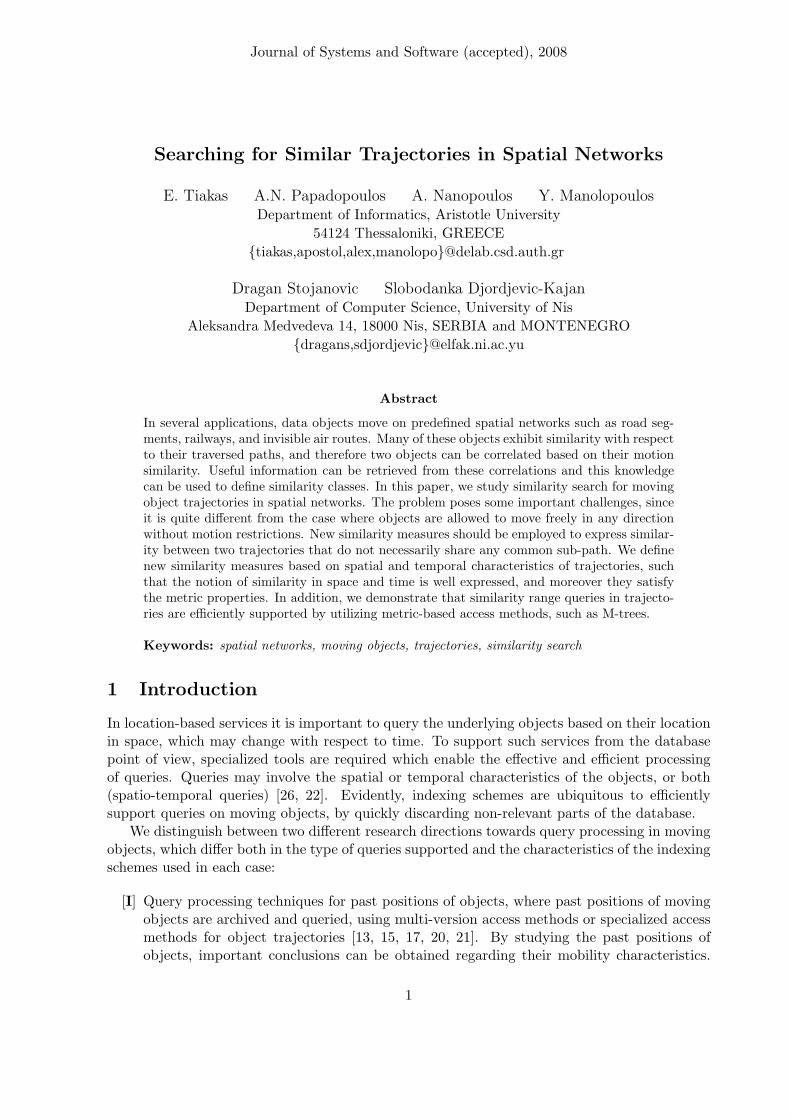
The common characteristic of the aforementioned approaches and research works is thatobjects are allowed to move freely in 2-D or 3-D space, without any motion restrictions. However,in a large number of applications, objects are allowed to move only on predefined paths ofan underlying network, resulting in constraint motion. For example, vehicles in a city canonly move on road segments. In such a case, the Euclidean distance between two movingobjects does not reflect their real distance. Figure 1 shows such an example which illustratesthe differences between restricted and unrestricted trajectories. Objects moving in a spatialnetwork follow specific paths determined by the graph topology, and therefore arbitrary motion isprohibited. This means that two trajectories which are similar regarding the Euclidean distancemay be dissimilar when the network distance is considered. The majority of existing methodsfor trajectory similarity assume that objects can move anywhere in the underlying space, andtherefore do not support motion constraints. Most of the proposals are inspired by the timeseries case, and provide translation invariance, which is not always meaningful in the case ofspatial networks. To attack this problem, the network is modeled as a directed graph, and thedistance between two objects is evaluated by using algorithms for shortest paths between thenodes of the graph.
Therefore, the challenge is to express trajectory similarity by respecting network constraints,which is also a strong motivation for the following real and practical applications:
2
x
yTrajectory Ta
Trajectory TbD
C
B
A
F L
K
E
G
I
J
H
Trajectory Ta
Trajectory Tb
(a) trajectories in Euclidean space (b) trajectories in a spatial network
Figure 1: Trajectories in (a) 2-D Euclidean space, and (b) in a spatial network.
[I] By identifying similar trajectories, effective data mining techniques (e.g., clustering) canbe applied to discover useful patterns. For example, a dense cluster is an indication ofemerge traffic measures, future road expansions, traffic-jam detection, traffic predictions,etc.
[II] Trajectory similarity can also help in several road network applications such as, routingapplications which support historical trajectories, logistic applications, city emergencyhandling, drive guiding systems, flow analysis etc. In such applications, efficient indexingand query processing techniques are required.
[III] Trajectory similarity of moving objects resembles path similarity of user click-streams inthe area of web usage mining. By analyzing the URL path of each user, we are able todetermine paths that are very similar, and therefore effective caching strategies can beapplied. In web usage mining, web pages and URL links are modeled as a graph. A nodein the graph represents a web page, and an edge from one page to another represents anexisting link between them. The time spent by each user to a page is also recorded, and itis used in expressing path similarity, in addition to the number of common web pages alongeach path. In the existing approaches, two paths are considered similar only if they shareat least one common web page, or if the paths contain web pages with similar concept. Intrajectory similarity on the other hand, two trajectories may be characterized similar evenif they do not share any nodes. Therefore, the existing web usage mining techniques arenot directly applicable, and the detection of network trajectory similarities can acceleratethe web usage mining queries.
The rest of the article is organized as follows. In the next section, we give the appropriatebackground, we present related work. In Section 3, trajectory similarity search is presented byinvestigating effective similarity measures between trajectories in a spatial network. Indexingand query processing issues are covered in Section 4, whereas Section 5 offers experimentalresults. Finally, Section 6 concludes the work.
2 Related Work
In several applications, the mobility of objects is constrained by an underlying spatial network.This means that objects cannot move freely, and their position must satisfy the network con-
3
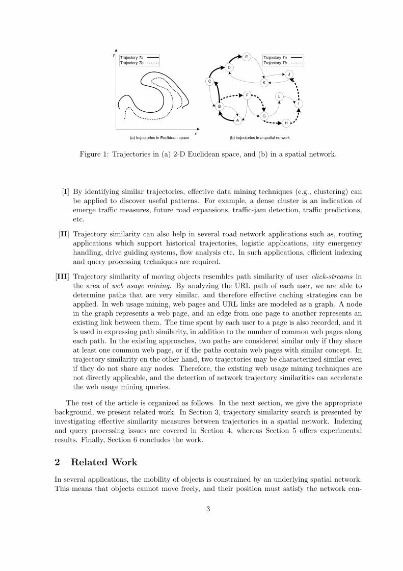
straints. Network connectivity is usually modeled by using a graph representation, composedof a set of vertices (nodes) and a set of edges (connections). Depending on the application,the graph may be weighted (a cost is assigned to each edge) and directed (each edge has anorientation). Figure 2 illustrates an example of a spatial network corresponding to a part of acity road network, and its graph representation.
v1
v2
v3
v5
v4
e1
e2
e3
e4
e5
e6
e7
e8
e9
v1
v2
v3
v5
v4
Figure 2: A road network and its graph representation.
Several research efforts have been performed towards efficient spatial and spatio-temporalquery processing in spatial networks. In [19] nearest-neighbor query processing is achieved byusing a mapping technique. This mapping transforms the graph representation of the networkto a high-dimensional space, where Minkowski metrics can be used. Nearest-neighbor queriesin road networks have been also studied in [7], where a graph representation is used to modelthe network. In [16] authors study query processing for stationary data sets, by using both agraph representation for the network and a spatial access method. It is shown that the use ofEuclidean distance retrieves many candidates, and instead they propose a network expansionmethod to process range, nearest-neighbor and join queries. In-route nearest-neighbor querieshave been studied in [29], where given a trajectory source and destination the smallest detouris calculated.
The above contributions deal with efficient spatial or spatio-temporal query processing offundamental queries like range, nearest-neighbor and join. However, the issue of trajectorysimilarity has not yet been studied adequately in the case of moving objects in spatial networks.Let Ta and Tb be the trajectories of moving objects oa and ob respectively, and D(Ta, Tb) afunction that expresses their dissimilarity in the range [0, 1]. If the two objects have similartrajectories we expect the value D(Ta, Tb) to be close to zero. On the other hand, if the twotrajectories are completely dissimilar, we expect the value D(Ta, Tb) to be close to one.
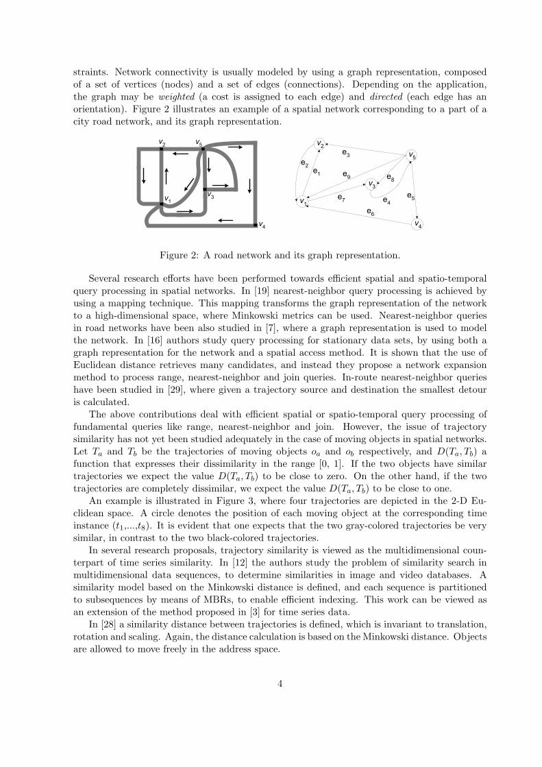
An example is illustrated in Figure 3, where four trajectories are depicted in the 2-D Eu-clidean space. A circle denotes the position of each moving object at the corresponding timeinstance (t1,...,t8). It is evident that one expects that the two gray-colored trajectories be verysimilar, in contrast to the two black-colored trajectories.
In several research proposals, trajectory similarity is viewed as the multidimensional coun-terpart of time series similarity. In [12] the authors study the problem of similarity search inmultidimensional data sequences, to determine similarities in image and video databases. Asimilarity model based on the Minkowski distance is defined, and each sequence is partitionedto subsequences by means of MBRs, to enable efficient indexing. This work can be viewed asan extension of the method proposed in [3] for time series data.
In [28] a similarity distance between trajectories is defined, which is invariant to translation,rotation and scaling. Again, the distance calculation is based on the Minkowski distance. Objectsare allowed to move freely in the address space.
4
x
y
t1
t2 t3t4t5t6 t7
t8
t1
t2t3
t4t5 t6 t7 t8
t1t2t3t4t5 t6 t7 t8
t1
t2
t3
t4
t5
t6t7
t8
Figure 3: Example of four trajectories in the 2-D Euclidean space.
In [14] an approach is studied to aggregate similar trajectories using a grid-based spatialunit aggregation. The notion of spatial similarity lies on the neighboring cells of the grid in astandard 2-dimensional Euclidean space. Many problems can be arisen with how the grid mustbe defined, what the cell dimensions must be, and in objects and clusters identification.
In [11] an efficient algorithm for trajectories similarity calculation is presented. But alldistance calculations through trajectories are based on Euclidean metrics and spaces (Lp norms).
The method proposed in [24, 25] employs a similarity distance based on the longest commonsubsequence (LCS) between two trajectories. This approach proposes a distance measure, whichis more immune to noise than the Minkowski distance, but does not satisfy the metric spaceproperties, and therefore it is difficult to exploit efficient indexing schemes. Instead, hierarchicalclustering is used to group trajectories. Moreover, the similarity measure depends heavily on twoparameters, namely δ and ε, which must be known in advance, and cannot be altered dynamicallywithout reorganization. These values determine the maximum distance between two locations ofdifferent trajectories, in time and space respectively, to be characterized as similar. Trajectoriesthat differ more are characterized as dissimilar and therefore their similarity is set to zero. Thisapproach does not permit the use of ranking or incremental computation of similarity nearest-neighbor queries.
To the best of the authors’ knowledge, the only research work studying trajectory similarityon networks is the work in [5, 6]. The authors propose a simple similarity measure based onPOIs (points of interest). They retrieve similar trajectories on road network spaces and notin Euclidean spaces. They propose a filtering method based on spatial similarity and refiningsimilar trajectories based on temporal distance. In order to determine the spatial similaritybetween trajectories, they define that two trajectories are similar in space by a set of pre-defined points of interest P if all points of P lie in both trajectories, otherwise they define thetwo trajectories as dissimilar. There are several drawbacks using this approach:
• The set of points of interest must be pre-defined and controlled by the user which is veryrestrictive.
• A simple wrong point selection in P can harm trajectory spatial similarity and the derivedsimilarity clusters, so points in P must be selected very carefully and by an expert of theused road network.
• The similarity in space with such definition (1=similar, 0=dissimilar) does not take intoaccount any notion of similarity percentage or similarity range. Therefore, we cannotdetermine how similar two trajectories are in space.
5

• The spatial similarity of two trajectories is based only into the fact that they share commonpoints, and not into the general network space. Therefore, many similarities excluded.For example, trajectories that have parallel edges with only a city block distance and nocommon points, are considered completely dissimilar.
In addition, no details are given with respect to the access methods required to provide efficientsimilarity search. Moreover, no discussion is performed regarding the metric space properties ofthe proposed distance measures. Our approach avoids all these drawbacks.
In the sequel, we study in detail the proposed similarity model for trajectory similarity searchin spatial networks aiming at: (i) the definition of similarity and distance measures betweentrajectories that satisfy the metric space properties, (ii) the exploitation of the distance betweentwo graph nodes, which is used as a building block for the definition of trajectory similarity,(iii) the incorporation of time information in the similarity metric, and (iv) the efficient supportof similarity queries by exploiting appropriate indexing schemes and applying fast processingalgorithms.
3 Trajectory Similarity Measures
Let T be a set of trajectories in a spatial network, which is represented by a graph G(V, E),where V is the set of nodes and E the set of edges. Each trajectory T ∈ T is defined as:
T = ((v1, t1) , (v2, t2) , ..., (vm, tm)) (1)
where m is the trajectory description length, vi denotes a node in the graph representation ofthe spatial network, and ti is the time instance (expressed in time units, e.g., seconds) that themoving object reached node vi, and t1 < ti < tm , ∀1 < i < m. It is assumed that movingfrom a node to another comes at a non-zero cost, since at least a small amount of time will berequired for the transition. Table 1 gives the most important symbols and the correspondingdefinitions that are used in our study.
3.1 Expressing Trajectory Similarity
We will follow a step-by-step construction of the similarity measure by first expressing similaritytaking into account only the visited path, ignoring time information. Time information will beconsidered in a subsequent step.
We begin our exploration by assuming that any two trajectories have the same descriptionlength. This assumption will be relaxed later. Let Ta and Tb be two trajectories, each ofdescription length m. By using our trajectory definition and ignoring the time information, wehave: Ta = (va1, va2, ..., vam) and Tb = (vb1, vb2, ..., vbm), where ∀i, vai ∈ V and vbi ∈ V .
Note that, to characterize two trajectories as similar it is not necessary that they sharecommon nodes. Therefore, the similarity measure must take into account the proximity of thetrajectories (how close is one trajectory with respect to the other).
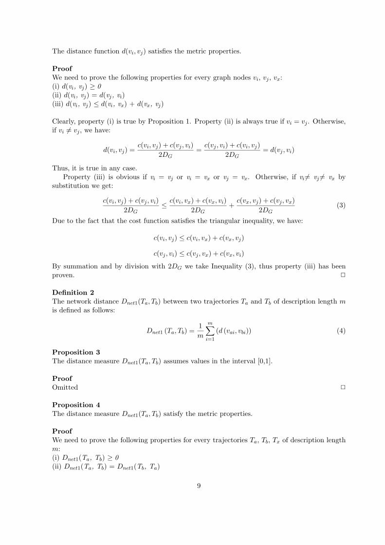
Due to motion restrictions posed by the spatial network, measuring trajectory proximityby means of the Euclidean distance is not appropriate. Instead, it is more natural to use thecost associated with each transition from a graph node to another. For example, in Figure 4we observe that two trajectory parts can be similar regarding the Euclidean distance, but maybe dissimilar regarding the shortest path distance (network-distance). Thus, for every pair ofpoints between these two trajectory parts, the Euclidean distance is small, but the corresponding
6
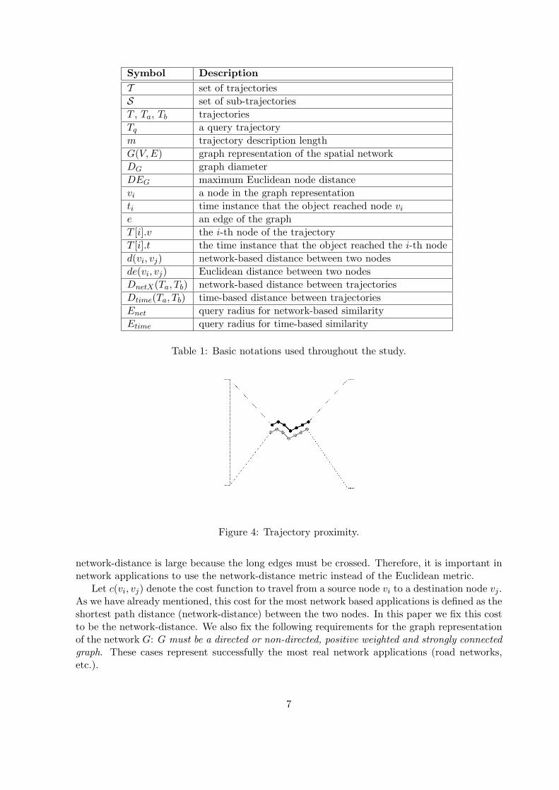
Symbol DescriptionT set of trajectoriesS set of sub-trajectoriesT , Ta, Tb trajectoriesTq a query trajectorym trajectory description lengthG(V, E) graph representation of the spatial networkDG graph diameterDEG maximum Euclidean node distancevi a node in the graph representationti time instance that the object reached node vi
e an edge of the graphT [i].v the i-th node of the trajectoryT [i].t the time instance that the object reached the i-th noded(vi, vj) network-based distance between two nodesde(vi, vj) Euclidean distance between two nodesDnetX(Ta, Tb) network-based distance between trajectoriesDtime(Ta, Tb) time-based distance between trajectoriesEnet query radius for network-based similarityEtime query radius for time-based similarity
Table 1: Basic notations used throughout the study.
Figure 4: Trajectory proximity.
network-distance is large because the long edges must be crossed. Therefore, it is important innetwork applications to use the network-distance metric instead of the Euclidean metric.
Let c(vi, vj) denote the cost function to travel from a source node vi to a destination node vj .As we have already mentioned, this cost for the most network based applications is defined as theshortest path distance (network-distance) between the two nodes. In this paper we fix this costto be the network-distance. We also fix the following requirements for the graph representationof the network G: G must be a directed or non-directed, positive weighted and strongly connectedgraph. These cases represent successfully the most real network applications (road networks,etc.).
7

The cost function (network distance) satisfies the following properties:
Property I: The cost function c(vi, vj) gives zero values if and only if vi ≡ vj .
It is obvious that c(v, v) = 0 for any node v in the graph representation. It also holds thatc(vi, vj) = 0 ⇒ vi ≡ vj , because it has been assumed that any transition between nodescomes at a non-zero cost (positive weighted graphs).
Property II: The cost function c(vi, vj), definitely satisfies the positivity property and thetriangular inequality:
• c(vi, vj) ≥ 0
• c(vi, vj) ≤ c(vi, vx) + c(vx, vj)
Property III: The cost function c(vi, vj), does not satisfy in general the symmetric property,therefore it is not definitely a metric function:
• c(vi, vj) 6= c(vj , vi)
But how does this reflect reality? Consider a directed road network with many one-wayroad segments, which is quite common. Then, it is clear that if a car goes from a sourcenode vi to a destination node vj , it will cover a distance generally different than its wayback from vj to vi, as it has to pass through different nodes with different weights.
3.1.1 Network Distance Measure 1
The first network distance measure Dnet1 that we propose uses network-based computations.The distance d(vi, vj) between any two nodes vi and vj , belonging to trajectories Ta and Tb
respectively, is given by the following definition.
Definition 1The distance d(vi, vj) between two graph nodes vi and vj is defined as follows:
d (vi, vj) =
{0 , if vi = vjc(vi,vj)+c(vj ,vi)
2DG, otherwise
(2)
where DG = max {c (vi, vj) , ∀vi, vj ∈ V (G)} is the diameter of the graph G of the spatial networkand is a global constant for the applications. Its value can be computed taking the overallmaximum of possible values of the cost function.
Proposition 1The distance function d(vi, vj) assumes values in the interval [0,1].
ProofThis is obvious when the function returns a zero value. Otherwise it returns the ratio c(vi,vj)+c(vj ,vi)
2DG.
But, clearly we have: c(vi, vj) ≤ DG and c(vj , vi) ≤ DG, and by summation we get: c(vi, vj) +c(vj , vi) ≤ 2DG. Therefore, by division we get: d (vi, vj) = c(vi,vj)+c(vj ,vi)
2DG≤ 1. In addition, we
have always c (vi, vj) ≥ 0 and c (vj , vi) ≥ 0 (positivity), thus d (vi, vj) ≥ 0. 2
Proposition 2
8
The distance function d(vi, vj) satisfies the metric properties.
ProofWe need to prove the following properties for every graph nodes vi, vj , vx:(i) d(vi, vj) ≥ 0(ii) d(vi, vj) = d(vj, vi)(iii) d(vi, vj) ≤ d(vi, vx) + d(vx, vj)
Clearly, property (i) is true by Proposition 1. Property (ii) is always true if vi = vj . Otherwise,if vi 6= vj , we have:
d(vi, vj) =c(vi, vj) + c(vj , vi)
2DG=
c(vj , vi) + c(vi, vj)2DG
= d(vj , vi)
Thus, it is true in any case.Property (iii) is obvious if vi = vj or vi = vx or vj = vx. Otherwise, if vi 6= vj 6= vx by
substitution we get:
c(vi, vj) + c(vj , vi)2DG
≤ c(vi, vx) + c(vx, vi)2DG
+c(vx, vj) + c(vj , vx)
2DG(3)
Due to the fact that the cost function satisfies the triangular inequality, we have:
c(vi, vj) ≤ c(vi, vx) + c(vx, vj)
c(vj , vi) ≤ c(vj , vx) + c(vx, vi)
By summation and by division with 2DG we take Inequality (3), thus property (iii) has beenproven. 2
Definition 2The network distance Dnet1(Ta, Tb) between two trajectories Ta and Tb of description length mis defined as follows:
Dnet1 (Ta, Tb) =1m
m∑
i=1
(d (vai, vbi)) (4)
Proposition 3The distance measure Dnet1(Ta, Tb) assumes values in the interval [0,1].
ProofOmitted 2
Proposition 4The distance measure Dnet1(Ta, Tb) satisfy the metric properties.
ProofWe need to prove the following properties for every trajectories Ta, Tb, Tx of description lengthm:(i) Dnet1(Ta, Tb) ≥ 0(ii) Dnet1(Ta, Tb) = Dnet1(Tb, Ta)
9

(iii) Dnet1(Ta, Tb) ≤ Dnet1(Ta, Tx) + Dnet1(Tx, Tb)Clearly, property (i) is true by consulting Proposition 3. Property (ii) is true because is alsotrue for the distance function d (Proposition 2), so:
Dnet (Ta, Tb) =1m
m∑
i=1
(d (vai, vbi)) =1m
m∑
i=1
(d (vbi, vai)) = Dnet (Tb, Ta)
Property (iii) is written equally by substitution:
1m
m∑
i=1
(d (vai, vbi)) ≤ 1m
m∑
i=1
(d (vai, vxi)) +1m
m∑
i=1
(d (vxi, vbi)) ⇔
⇔m∑
i=1
(d (vai, vbi)) ≤m∑
i=1
(d (vai, vxi)) +m∑
i=1
(d (vxi, vbi)) (5)
From Proposition 2 we have the following inequalities:
d (vai, vbi) ≤ d (vai, vxi) + d (vxi, vbi) , ∀i ∈ {1, 2, ..., m}
By summation we get (5). 2
Figure 5 shows two trajectories Ta, Tb for which we are interested to calculate their distance.Assuming that DG = 100, we have the following calculations:
d(vai, vbi) ={
17200
,16200
,9
200,
7200
, 0,5
200,
13200
}
Dnet1 (Ta, Tb) =17
(17200
+16200
+9
200+
7200
+ 0 +5
200+
13200
)=
17
67200
= 0.047857
3.1.2 Network Distance Measure 2
The second distance measure, Dnet2, that we propose uses an Euclidean-based distance function(de) in combination with the previous global constant DG (the graph diameter by the networkdistance). It can be used for fast calculations only for graphs where the coordinates of the nodesare available. In fact, in many cases the Euclidean distance results in poor performance regarding
Figure 5: Trajectory similarity example.
10
the quality of results. However, as it will be described later, it offers a “quick-and-dirty” viewof the results.
Definition 6The distance de(vi, vj) between two graph nodes vi and vj is defined as follows:
de (vi, vj) =euclidean(vi, vj)
DG=
√(xvi − xvj
)2+
(yvi − yvj
)2
DG(6)
where xvi , yvi are the coordinates of node vi, and xvj , yvj are the coordinates of node vj .
Proposition 7The distance function de(vi, vj) assumes values in the interval [0,1].
ProofLet DEG be the maximum Euclidean distance between all nodes of the graph representing thespatial network: DEG = max {euclidean(vi, vj), ∀vi, vj ∈ V (G)}. Then it is obvious that:
euclidean(vi, vj) ≤ DEG ≤ DG, ∀vi, vj ∈ V (G)
The last inequality holds because all network distances are always greater than or equal to thecorresponding Euclidean distances. Therefore, we have:
euclidean(vi, vj)DG
≤ 1 ⇔ de(vi, vj) ≤ 1
Moreover, as all distances are positive (or zero when vi = vj), we have always: de(vi, vj) ≥ 0. 2
Proposition 8The distance function de(vi, vj) satisfies the metric properties.
ProofDue to the fact that the Euclidean distance euclidean(vi, vj) satisfies the metric propertiesand de(vi, vj) is the Euclidean distance divided by the positive constant DG, it is evident thatde(vi, vj) also satisfies the metric properties. 2
Definition 7The network distance Dnet2(Ta, Tb) between two trajectories Ta and Tb of description length mis defined as follows:
Dnet2 (Ta, Tb) =1m
m∑
i=1
(de (vai, vbi)) (7)
Proposition 9The distance measure Dnet2(Ta, Tb) assumes values in the interval [0,1].
ProofOmitted 2
Proposition 10
11
The distance measure Dnet2(Ta, Tb) satisfy the metric properties.
ProofOmitted 2
3.2 Incorporating Time Information
The similarity measures defined in the previous section take into consideration only the travelingcost information, which depends on the spatial network. In applications such as traffic analysis,the time information associated with each trajectory is also very important.
Definition 8Given two trajectories Ta ∈ T and Tb ∈ T of description length m, their distance with respectto time Dtime(Ta, Tb) is given by:
Dtime (Ta, Tb) =1
m− 1
m−1∑
i=1
|(Ta [i + 1] .t− Ta [i] .t)− (Tb [i + 1] .t− Tb [i] .t)|max {(Ta [i + 1] .t− Ta [i] .t) , (Tb [i + 1] .t− Tb [i] .t)}
Essentially, the time similarity between two trajectories, as it has been defined, measurestheir resemblance with respect to the time required to travel from one node to the next (inter-arrival times).
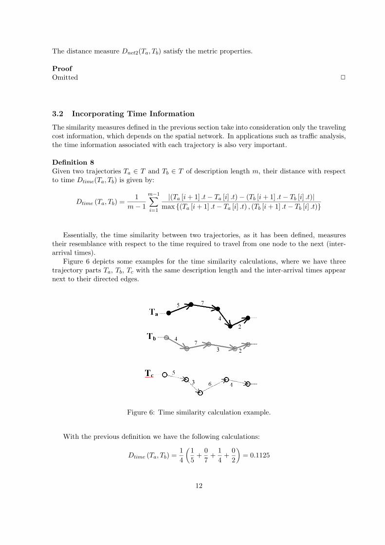
Figure 6 depicts some examples for the time similarity calculations, where we have threetrajectory parts Ta, Tb, Tc with the same description length and the inter-arrival times appearnext to their directed edges.
Figure 6: Time similarity calculation example.
With the previous definition we have the following calculations:
Dtime (Ta, Tb) =14
(15
+07
+14
+02
)= 0.1125
12
Dtime (Ta, Tc) =14
(05
+47
+26
+24
)= 0.35119
We observe that Ta is more similar to Tb than Tc and this happens because the correspondinginter-arrival times of the pair Ta, Tb are much closer.
Proposition 11The distance measure Dtime(Ta, Tb) assumes values in the interval [0,1].
ProofOmitted 2
Proposition 12The distance measure Dtime(Ta, Tb) satisfy the metric properties.
ProofWe need to prove the following properties for any trajectories Ta, Tb, Tx of description length m:
(i) Dtime(Ta, Tb) ≥ 0
(ii) Dtime(Ta, Tb) = Dtime(Tb, Ta)
(iii) Dtime(Ta, Tb) ≤ Dtime(Ta, Tx) + Dtime(Tx, Tb)
Clearly, property (i) is true by Proposition 11. Let us denote the inter-arrival times of alltrajectory parts Ta, Tb and Tx as follows: δai = Ta[i + 1].t− Ta[i].t, δbi = Tb[i + 1].t− Tb[i].t andδxi = Tx[i + 1].t− Tx[i].t, for all i=1,2,...,m-1. Then, property (ii) is true because we have:
Dtime (Ta, Tb) =1
m− 1
m−1∑
i=1
|δai − δbi|max {δai, δbi} =
1m− 1
m−1∑
i=1
|δbi − δai|max {δbi, δai} = Dtime (Tb, Ta)
By substitution, property (iii) is written as:
1m− 1
m−1∑
i=1
|δai − δbi|max {δai, δbi} ≤
1m− 1
m−1∑
i=1
|δai − δxi|max {δai, δxi} +
1m− 1
m−1∑
i=1
|δxi − δbi|max {δxi, δbi} ⇔
⇔m−1∑
i=1
|δai − δbi|max {δai, δbi} ≤
m−1∑
i=1
|δai − δxi|max {δai, δxi} +
m−1∑
i=1
|δxi − δbi|max {δxi, δbi} (8)
It is sufficient to prove the following inequalities ∀ i = 1, . . . , m-1:
|δai − δbi|max {δai, δbi} ≤
|δai − δxi|max {δai, δxi} +
|δxi − δbi|max {δxi, δbi} (9)
To prove 9 it is enough to prove that for every positive numbers a, b, c the following holds:
|a− b|max {a, b} ≤
|a− c|max {a, c} +
|c− b|max {c, b} (10)
But, this inequality is obvious if a = b, or a = c, or b = c, and for all other ordering cases ofthe numbers a, b, c also holds:
13

• if a < b < c then it gives:
b− a
b≤ c− a
c+
c− b
c⇔ c(b− a) ≤ b(c− a) + b(c− b) ⇔ (b + a)(c− b) ≥ 0
which it holds as a, b are positive and b < c.
• if a < c < b then it gives:
b− a
b≤ c− a
c+
b− c
b⇔ c(b− a) ≤ b(c− a) + c(b− c) ⇔ (c− a)(b− c) ≥ 0
which it holds as a < c and c < b.
• if b < a < c then it gives:
a− b
a≤ c− a
c+
c− b
c⇔ c(a− b) ≤ a(c− a) + a(c− b) ⇔ (a + b)(c− a) ≥ 0
which it holds as a, b are positive and a < c.
• if b < c < a then it gives:
a− b
a≤ a− c
a+
c− b
c⇔ c(a− b) ≤ c(a− c) + a(c− b) ⇔ (c− b)(a− c) ≥ 0
which it holds as b < c and c < a.
• if c < a < b then it gives:
b− a
b≤ a− c
a+
b− c
b⇔ a(b− a) ≤ b(a− c) + a(b− c) ⇔ (a + b)(a− c) ≥ 0
which it holds as a, b are positive and c < a.
• if c < b < a then it gives:
a− b
a≤ a− c
a+
b− c
b⇔ b(a− b) ≤ b(a− c) + a(b− c) ⇔ (a + b)(b− c) ≥ 0
which it holds as a, b are positive and c < b.
Therefore, Inequality (10) is true, and property (iii) has been proven. 2
3.2.1 Spatio-temporal Similarity Measures and Methods
We have at hand different distance measures, Dnet and Dtime, that can be used to compare tra-jectories of the same length in space and time. Several applications may require both similaritymeasures to extract useful knowledge.
There are three different methods in order to retrieve similar trajectories in space-time asproposed in [5]: (i) Searching similar trajectories with direct application of spatio-temporaldistance measures, (ii) Filtering trajectories based on temporal similarity and refining similartrajectories based on spatial distance, (iii) Filtering trajectories based on spatial similarity andrefining similar trajectories based on temporal distance.
Here we suggest the methods (i) and (iii), due to the fact that method (ii) can hardly befound in practical applications.
14
To implement method (i) we can combine the two distance measures Dnet and Dtime into asingle one. For example, the two distances may be weighted with parameters Wnet and Wtime
such that Wnet+Wtime=1. The total (combined) distance can then be expressed as follows:
Dtotal (Ta, Tb) = Wnet ·Dnet (Ta, Tb) + Wtime ·Dtime (Ta, Tb)
It is evident that the distance measure Dtotal satisfies the metric space properties. However,this approach poses a significant limitation, since the values of Wnet and Wtime must be knownin advance.
Consequently we propose method (iii) using Dnet and Dtime separately, where the distanceDnet making the filtering step in space and the distance Dtime making the refinement step intime. In this way, two parameter distances are required to be posed by the query. The distanceEnet expresses the desired similarity with respect to the Dnet distance measure, whereas thedistance Etime expresses the desired similarity regarding the Dtime distance measure. If the userwishes to focus only on the network distance, then the value of Etime may be set to 1. Otherwise,another value is required for Etime, which determines the desired similarity in the time domain.By allowing the user to control the values of Enet and Etime a significant degree of flexibility isachieved, since the “weight” of each distance can be controlled at will.
4 Indexing and Query Processing Issues
In this section, we study some important issues regarding trajectory similarity. Firstly, wediscuss the problem of handling trajectories of different description length, by decomposing atrajectory to sub-trajectories. Then, we study the use of indexing schemes for sub-trajectories.Finally, we study some fundamental query processing issues.
4.1 Trajectory Decomposition
Up to now we have handled the case where all trajectories are of the same description length.We proceed now to relax this assumption, by considering trajectories of different lengths. Infact, this is the more general case that reflects reality. First of all, two trajectories may involvea different number of visited nodes, and therefore their description length will be different.Furthermore, we cannot always guarantee that moving objects report their positions at fixedtime intervals. Due to noise, several measurements may be lost, or different moving objectsreport their positions at different time intervals. In these cases, two trajectories may havedifferent description lengths.
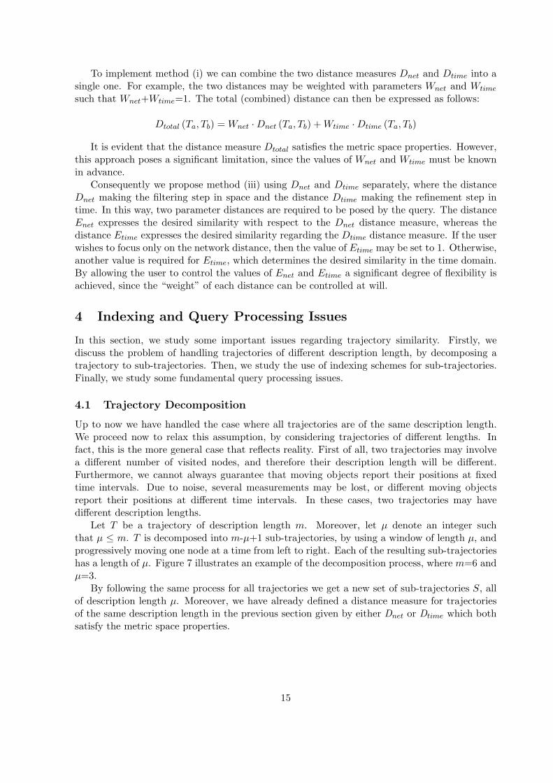
Let T be a trajectory of description length m. Moreover, let µ denote an integer suchthat µ ≤ m. T is decomposed into m-µ+1 sub-trajectories, by using a window of length µ, andprogressively moving one node at a time from left to right. Each of the resulting sub-trajectorieshas a length of µ. Figure 7 illustrates an example of the decomposition process, where m=6 andµ=3.
By following the same process for all trajectories we get a new set of sub-trajectories S, allof description length µ. Moreover, we have already defined a distance measure for trajectoriesof the same description length in the previous section given by either Dnet or Dtime which bothsatisfy the metric space properties.
15
1 2 3 4 5 6
5 7 10 15 21 30
(1,5), (2,7), (3,10), (4,15), (5,21), (6,30)
1 2 3
5 7 10
2 3 4
7 10 15
3 4 5
10 15 21
4 5 6
15 21 30
T
S1
S2
S3
S4
(1,5), (2,7), (3,10)
(2,7), (3,10), (4,15)
(3,10), (4,15), (5,21)
(4,15), (5,21), (6,30)
Figure 7: Trajectory decomposition example for m = 6 and µ = 3.
4.2 Indexing Schemes
Our next step involves indexing the set S of sub-trajectories, enabling efficient query processing.Towards this direction, we propose two schemes, which are both based on the M-tree accessmethod [2]. Note that since a vector representation of each sub-trajectory is not available,techniques like R-trees [4] and its variants are not applicable. Recall that, the M-tree is alreadyequipped by the necessary tools to handle range and nearest-neighbor queries, as it has beenreported in [2]. The only requirement for the M-tree to work properly is that the distance usedmust satisfy the metric space properties. Since both Dnet and Dtime satisfy these properties,they can be used as distance measures in M-trees. Note that, among the metric indexing schemeswe choose the M-tree because of its simplicity. However, other secondary memory schemes formetric spaces or any other metric access method can been applied equally well (e.g., SlimTrees[23]). Two alternatives are followed towards indexing sub-trajectories:
• M-treeI method. In this scheme, only the NET-M-tree is used to check the constraintregarding Enet. Then, in a subsequent step the candidate sub-trajectories are checkedagainst the time constraints. This way, only one M-tree is used.
• M-treeII method. In this scheme, two M-trees are used to handle Dnet and Dtime
separately. These trees are termed NET-M-tree and TIME-M-tree respectively. Each M-tree is searched separately using Enet and Etime respectively. Then, the intersection ofboth results is determined to get the sub-trajectories that satisfy the network and timeconstraints.
16
4.3 Query Processing Fundamentals
A user query is defined by a triplet < Tq, Enet, Etime > where Tq is the query trajectory, Enet isthe radius for the network distance and Etime is the radius for the time distance. For the queryprocessing to be consistent with the proposed framework, each query trajectory Tq must be ofat least description length µ. If this is not true, padding is performed by repeating, for example,the last node of the trajectory several times, until the description length µ is reached. In thegeneral case where the description length of Tq is greater than µ, the decomposition process isapplied to obtain the sub-trajectories of Tq. Finally, if the description length of Tq is equal toµ, then only one sub-trajectory is produced.
Let p denote the number of sub-trajectories of Tq determined by the trajectory decompositionprocess. The next step depends on the indexing scheme we utilize, i.e. either M-treeI or M-treeIIas they have been described previously. A trajectory is part of the answer if there is at leastone of its sub-trajectories that satisfy the network and time constraints for at least one querysub-trajectory. In the sequel, we analyze the whole process in detail:
• Having a query trajectory Tq of description length l and the Enet, Etime parameters, wedecompose Tq into p = l - µ + 1 sub-trajectories (if l > µ) with the window method andthen we construct their set QS(Tq).
• For every query sub-trajectory qs ∈ QS(Tq), we execute a simple range query to NET-M-Tree with radius Enet and collect related sub-trajectories into the set Cnet.
• If M-treeII method is used then we execute another simple range query to TIME-M-Treewith radius Etime and collect related sub-trajectories into the set Ctime.
• If M-treeI method is used then we check every sub-trajectory in Cnet against Etime andfrom the selected results we construct the set AS. Otherwise, If M-treeII method is used,the results’ set AS is constructed with the common sub-trajectories of the sets Cnet andCtime. In both cases, the set AS contains the resulted sub-trajectories ID’s.
• From the set AS we take the corresponding trajectories ID’s and we construct the finalresult set AT .
In any case, a trajectory T ∈ T will appear in the result set, if and only if there exists atleast one sub-trajectory ts of T which is similar to at least one sub-trajectory qs of the querytrajectory Tq, and also satisfies the network and time constraints. More formally:
T is similar to Tq ⇔ ∃ts ⊆ T,∃qs ⊆ Tq : Dnet(ts, qs) ≤ Enet ∧Dtime(ts, qs) ≤ Etime
Figure 8 presents an outline of the algorithm. Taking into account that the consecutivesub-trajectories of Tq have (µ - 1) common nodes, most calculations and requests can be alreadyin the memory, as we check one sub-trajectory after another, so it is strongly recommended touse an LRU memory buffer.
4.4 Distance Buffering
The distance measure Dnet1 uses the shortest path distance between graph nodes. These com-putations can be performed more efficiently by using an LRU buffer. The LRU buffer maintainsa constant amount of distance values into main memory. In the experimental results section we
17

Algorithm SimilaritySearch(Tq, Enet, Etime, µ)InputTq: query trajectoryEnet: network distance radiusEtime: time distance radiusµ: minimum description length of query sub-trajectoryOutputAS: set of sub-trajectory IDsAT : set of trajectory IDs
1. QS(Tq) = all sub-trajectories of Tq of description length µ2. for each query sub-trajectory qs ∈ QS(Tq)3. if method M-treeI is used then4. search NET-M-tree using qs and Enet
5. Cnet = candidate sub-trajectories from NET-M-tree6. check every sub-trajectory in Cnet against Etime
7. update AS8. else if method M-treeII is used then9. search NET-M-tree using qs and Enet
10. Cnet = candidate sub-trajectories from NET-M-tree11. search TIME-M-tree using qs and Etime
12. Ctime = candidate sub-trajectories from TIME-M-tree13. AS = Cnet ∩ Ctime
14. end if15. end for16. calculate AT from AS17. return(AS,AT )
Figure 8: Outline of similarity search algorithm.
show that only a relatively small buffer size is adequate to accelerate performance, offering agood hit-ratio.
If the network graph has at most a few thousand nodes, it is suggested to precompute alldistances c(vi, vj) between nodes and to put them into a hash-based file. Then, the LRU memorybuffer can cooperate with this file during the request procedure for even better performance.Later, we discuss the alternative of storing only a subset of precomputed distances on the disk,to handle large graphs.
The algorithm in Figure 9 illustrates the process of retrieving a distance c(vi, vj). Thevariables requests, hits, and misses are used to test buffer performance.
It is important to remind that the LRU memory buffer and the precomputed distances diskfile, are used only with Dnet1. They are not necessary for Dtime calculations and in Dnet2
measure which does not use network distances at all.
4.5 Combining Measures Dnet1 and Dnet2 (Filtering and Refinement)
Due to network restrictions, a similarity range query using the Dnet2 distance measure mayreturn some trajectories that are not similar regarding distance measure Dnet1 (false alarms).This effect is more significant when the shortest path distance between nodes is considerablyhigher than their Euclidean distance. Therefore, we need to detect these trajectories usinganother measure, which respects the network restrictions in space, and use it in a refinementstep during query processing. For this reason, we can select the distance measure Dnet1 to handlefalse alarm detection. This procedure will give correct results if and only if we prove that every
18
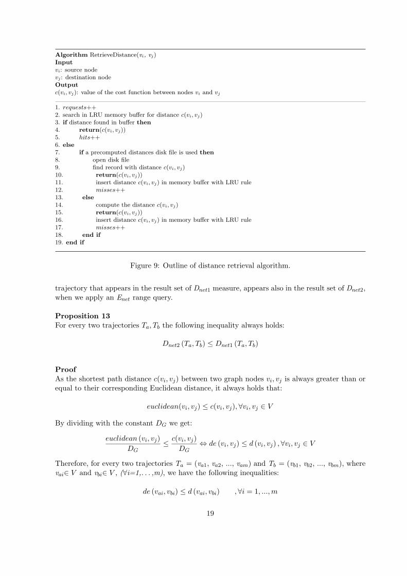
Algorithm RetrieveDistance(vi, vj)Inputvi: source nodevj : destination nodeOutputc(vi, vj): value of the cost function between nodes vi and vj
1. requests++2. search in LRU memory buffer for distance c(vi, vj)3. if distance found in buffer then4. return(c(vi, vj))5. hits++6. else7. if a precomputed distances disk file is used then8. open disk file9. find record with distance c(vi, vj)10. return(c(vi, vj))11. insert distance c(vi, vj) in memory buffer with LRU rule12. misses++13. else14. compute the distance c(vi, vj)15. return(c(vi, vj))16. insert distance c(vi, vj) in memory buffer with LRU rule17. misses++18. end if19. end if
Figure 9: Outline of distance retrieval algorithm.
trajectory that appears in the result set of Dnet1 measure, appears also in the result set of Dnet2,when we apply an Enet range query.
Proposition 13For every two trajectories Ta, Tb the following inequality always holds:
Dnet2 (Ta, Tb) ≤ Dnet1 (Ta, Tb)
ProofAs the shortest path distance c(vi, vj) between two graph nodes vi, vj is always greater than orequal to their corresponding Euclidean distance, it always holds that:
euclidean(vi, vj) ≤ c(vi, vj), ∀vi, vj ∈ V
By dividing with the constant DG we get:
euclidean (vi, vj)DG
≤ c(vi, vj)DG
⇔ de (vi, vj) ≤ d (vi, vj) , ∀vi, vj ∈ V
Therefore, for every two trajectories Ta = (va1, va2, ..., vam) and Tb = (vb1, vb2, ..., vbm), wherevai∈ V and vbi∈ V , (∀i=1,. . . ,m), we have the following inequalities:
de (vai, vbi) ≤ d (vai, vbi) ,∀i = 1, ...,m
19
By summation, we get:
m∑
i=1
(de (vai, vbi)) ≤m∑
i=1
(d (vai, vbi))
⇔ 1m
m∑
i=1
(de (vai, vbi)) ≤ 1m
m∑
i=1
(d (vai, vbi))
⇔ Dnet2 (Ta, Tb) ≤ Dnet1 (Ta, Tb)
and the proposition has been proven. 2
Following Proposition 13, when we have a query trajectory Tq and a network query range Enet,all trajectories returned by Dnet1 measure will appear in the result-set of Dnet2, because:
Dnet2 (Tq, T ) ≤ Dnet1 (Tq, T ) ≤ Enet , ∀T ∈ T
Figure 10 illustrates the outline of the similarity search algorithm including the refinementstep. Dnet2 is used as the filtering distance measure, whereas Dnet1 is used for refinement, toeliminate false alarms. An important observation is that this scheme can be applied to bothM-treeI and M-treeII methods, and moreover, it can be used with any well-defined distancemeasure, as long as the following lower-bounding property holds:
Dfiltering (Ta, Tb) ≤ Drefinement (Ta, Tb) , ∀Ta, Tb ∈ T
5 Performance Evaluation
In this section, we give information about the implementation of the proposed approach in C++and the results of experiments that confirm and evaluate all previous algorithms, procedures andtechniques. All experiments have been conducted on a Pentium IV running Windows XP, with1GB of RAM, and a 320GB-SATA2-16MB hard disk. First, we present the construction ofused spatial network and trajectory data set. Then, we present the construction of M-Trees foreach defined measure and how the proposed measures express well the notion of similarity inspace and time. At the main part, we present the evaluation results of all proposed methods forsimilarity range queries.
5.1 Spatial Network Data
All experiments have been conducted using a real-world spatial network, the road network ofOldenburg city [1]. The cost function c(vi, vj) between two nodes of the graph representation isthe shortest path distance. The number of vertices in the Oldenburg data set is 6,105. Therefore,the total number of precomputed distances among all possible pairs of vertices is 37,271,025.These distances are stored in a hash-based file on disk (DISTfile), using the Hilbert space fillingcurve as a hashing function. The Hilbert curve values are derived from the corresponding sourceand target node ID’s of the distances, which are integers into the interval [0, |VG| − 1], (e.g.,for the distance c(vi, vj) the value Hilbert(ID(vi), ID(vj)) is calculated). For the selected road
20

Algorithm SimilaritySearchWithRefinement(Tq, Enet, Etime, µ)InputTq: query trajectoryEnet: network distance radiusEtime: time distance radiusµ: minimum description length of query sub-trajectoryOutputASF : final set of sub-trajectory IDsATF : final set of trajectory IDs
1. QS(Tq) = all sub-trajectories of Tq of description length µ2. ASF=Ø3. for each query sub-trajectory qs ∈ QS(Tq)4. if method M-treeI is used5. search NET-M-tree (constructed by the basic metric) using qs and Enet
6. Cnet = candidate sub-trajectories from NET-M-tree (using the Dnet distance of the basic metric)7. check every sub-trajectory in Cnet against Etime
8. update AS9. else if method M-treeII is used then10. search NET-M-tree (constructed by the basic metric) using qs and Enet
11. Cnet = candidate sub-trajectories from NET-M-tree (using the Dnet distance of the basic metric)12. search TIME-M-tree using qs and Etime
13. Ctime= candidate sub-trajectories from TIME-M-tree14. AS = Cnet ∩ Ctime
15. end if16. for each sub-trajectory Si in AS17. compute the Dnet distance of Si from qs using the selected refinement metric18. insert Si in ASF if that distance is less than or equal to Enet
19. end for20. end for21. calculate ATF from ASF22. return(ASF ,ATF )
Figure 10: Outline of similarity search algorithm with refinement step.
network, the total time required for all precomputations and creation of DISTfile is 3,180.581sec. The record length has been set to 16 bytes, so the final file capacity is 596,336,400 bytes(285MB zipped).
An in-core LRU buffer has been used to keep a number of precomputed distances in mainmemory (we initialized the buffer selecting some top-used distances through calculations whichactually are distances between nodes that included in the most trajectory parts). The size ofthe buffer has been set to 2,000, which is a relatively small value compared to the total numberof pair-wise distances. We have computed the average number of network distance calculationrequests, the average number of hits and misses, in simple range queries in space using Dnet1
and Dnet2. The results show that almost 85% of the distance requests are absorbed by the mainmemory buffer and therefore, we avoid fetching them from the disk. The more buffer pages areavailable, the higher the hit ratio becomes.
The fast retrieval of shortest path distances is the most time consuming factor affecting theperformance of network-based distance calculations, the construction of M-Trees and finally inthe performance of similarity range queries.
21
5.2 Construction of Trajectories and Sub-trajectories
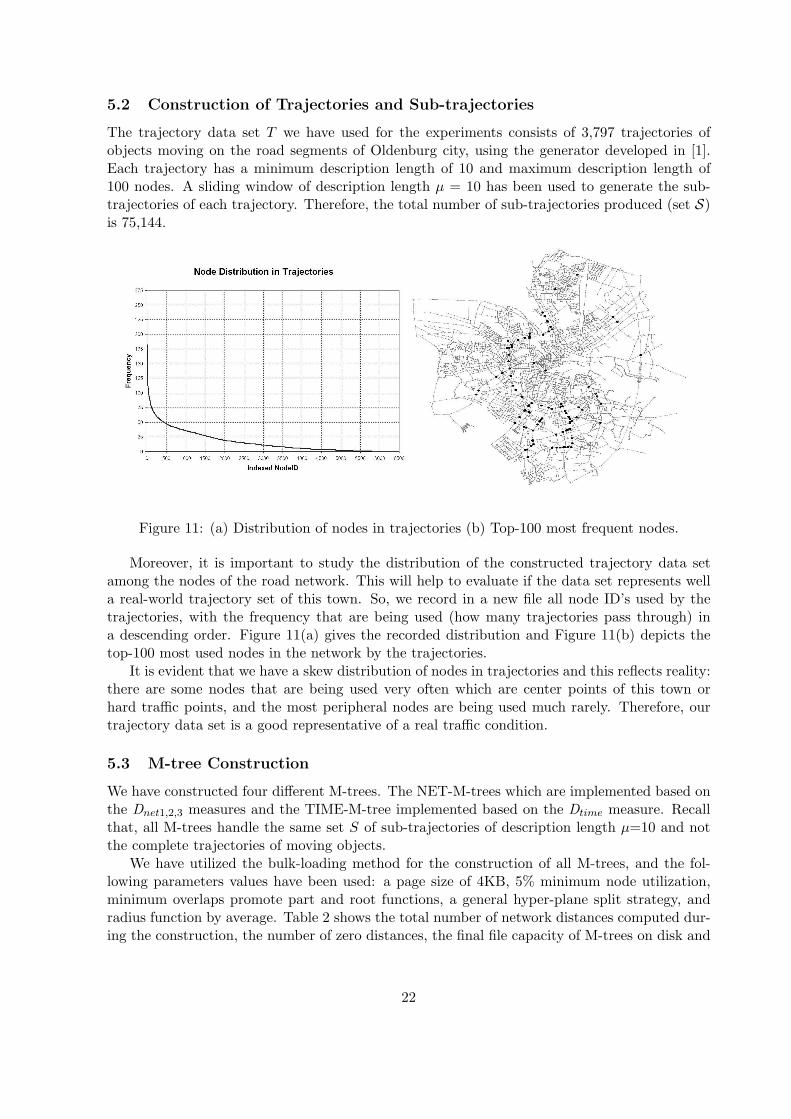
The trajectory data set T we have used for the experiments consists of 3,797 trajectories ofobjects moving on the road segments of Oldenburg city, using the generator developed in [1].Each trajectory has a minimum description length of 10 and maximum description length of100 nodes. A sliding window of description length µ = 10 has been used to generate the sub-trajectories of each trajectory. Therefore, the total number of sub-trajectories produced (set S)is 75,144.
Figure 11: (a) Distribution of nodes in trajectories (b) Top-100 most frequent nodes.
Moreover, it is important to study the distribution of the constructed trajectory data setamong the nodes of the road network. This will help to evaluate if the data set represents wella real-world trajectory set of this town. So, we record in a new file all node ID’s used by thetrajectories, with the frequency that are being used (how many trajectories pass through) ina descending order. Figure 11(a) gives the recorded distribution and Figure 11(b) depicts thetop-100 most used nodes in the network by the trajectories.
It is evident that we have a skew distribution of nodes in trajectories and this reflects reality:there are some nodes that are being used very often which are center points of this town orhard traffic points, and the most peripheral nodes are being used much rarely. Therefore, ourtrajectory data set is a good representative of a real traffic condition.
5.3 M-tree Construction
We have constructed four different M-trees. The NET-M-trees which are implemented based onthe Dnet1,2,3 measures and the TIME-M-tree implemented based on the Dtime measure. Recallthat, all M-trees handle the same set S of sub-trajectories of description length µ=10 and notthe complete trajectories of moving objects.
We have utilized the bulk-loading method for the construction of all M-trees, and the fol-lowing parameters values have been used: a page size of 4KB, 5% minimum node utilization,minimum overlaps promote part and root functions, a general hyper-plane split strategy, andradius function by average. Table 2 shows the total number of network distances computed dur-ing the construction, the number of zero distances, the final file capacity of M-trees on disk and
22
M-tree Distances Zeros Capacity TimeDnet1 1,574,890 38,309 32.5MB 13min+7secDnet2 1,494,416 37,761 32.1MB 35secDtime 4,013,864 40,461 30.9MB 1min+46sec
Table 2: Information regarding the construction of M-trees.
the total construction time. Note that we have exploited precomputed distances (LRU-bufferand DISTfile) during the construction procedure.
We observe that Dnet2 gives the smallest capacity and construction time, because networkdistance computations are not required.
5.4 Evaluation of Similarity Measures
We have randomly selected several trajectories from different areas of Oldenburg and we haveperformed similarity range queries by using all measures.
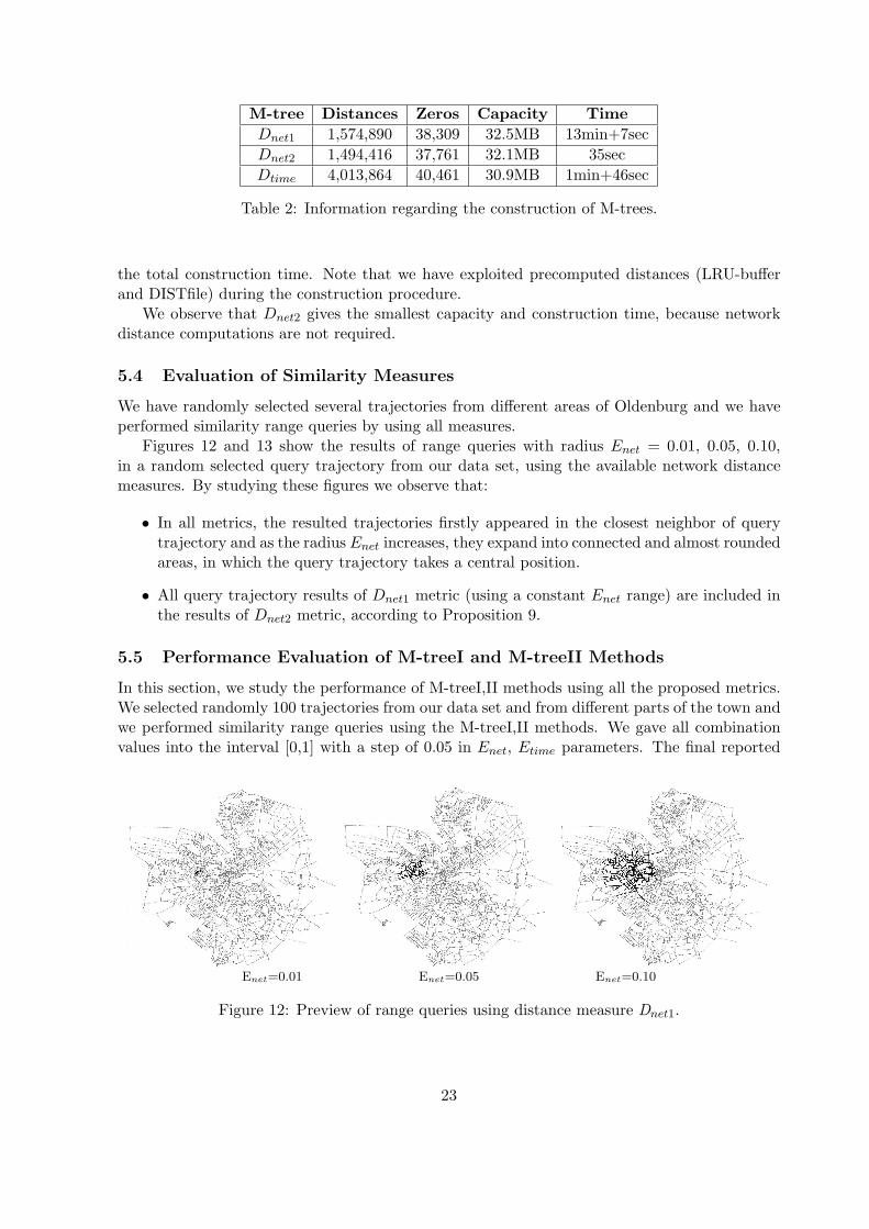
Figures 12 and 13 show the results of range queries with radius Enet = 0.01, 0.05, 0.10,in a random selected query trajectory from our data set, using the available network distancemeasures. By studying these figures we observe that:
• In all metrics, the resulted trajectories firstly appeared in the closest neighbor of querytrajectory and as the radius Enet increases, they expand into connected and almost roundedareas, in which the query trajectory takes a central position.
• All query trajectory results of Dnet1 metric (using a constant Enet range) are included inthe results of Dnet2 metric, according to Proposition 9.
5.5 Performance Evaluation of M-treeI and M-treeII Methods
In this section, we study the performance of M-treeI,II methods using all the proposed metrics.We selected randomly 100 trajectories from our data set and from different parts of the town andwe performed similarity range queries using the M-treeI,II methods. We gave all combinationvalues into the interval [0,1] with a step of 0.05 in Enet, Etime parameters. The final reported
Enet=0.01 Enet=0.05 Enet=0.10
Figure 12: Preview of range queries using distance measure Dnet1.
23

Enet=0.01 Enet=0.05 Enet=0.10
Figure 13: Preview of range queries using distance measure Dnet2.
Variable DescriptionNnet Number of similar sub-trajectories found in NET-M-treeDnet Number of network-based distance computationsTnet Total searching time in NET-M-tree (sec)MBFR Memory LRU Buffer Total RequestsMBFH Memory LRU Buffer Total HitsMBFM Memory LRU Buffer Total MissesDBFR Disk LRU Buffer Total RequestsDBFH Disk LRU Buffer Total HitsDBFM Disk LRU Buffer Total MissesNtime Number of similar sub-trajectories found in TIME-M-treeDtime Number of time-based distance computationsTtime Total searching time in TIME-M-tree (M-treeII) or in time calcula-
tions (M-treeI) (sec)TT Total query timeAS Total number of common (M-treeII) or accepted (M-treeI) sub-
trajectories found (Net&Time)AT Total number of similar trajectories found (final results)FA False alarms for sub-trajectories in Dnet2+1 method
Table 3: Basic variables measured throughout experiments.
results correspond to the average values of these 100 queries. The basic parameters that arestudied are summarized in Table 3.
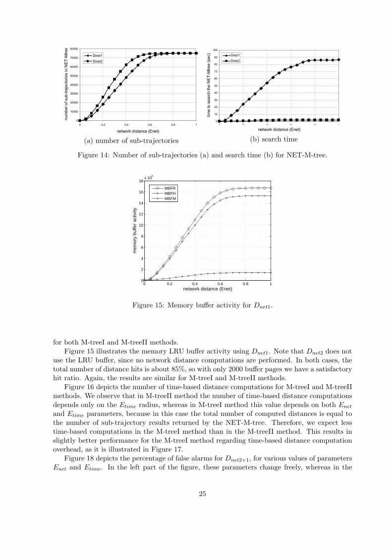
Figure 14(a) depicts the number of similar sub-trajectories found using all available network-based distance measures. Recall, that the results are the same for both M-treeI and M-treeIImethods. As the Enet radius increases, Dnet2 first reaches the upper limit (75,144), followedby Dnet1. Evidently, the distance measure Dnet2 gives more results than Dnet1 due to thelower-bounding property.
Figure 14(b) depicts the total time spent for network-based computations using all network-based distance measures. It is evident that Dnet2 is the less time-consuming measure sincedistances are computed by using the Euclidean distance of the nodes. The results are similar
24
0
10000
20000
30000
40000
50000
60000
70000
80000
0 0,2 0,4 0,6 0,8 1
network distance (Enet)
nu
mb
er
of
su
b-t
raje
cto
rie
s i
n N
ET
-Mtr
ee
Dnet1
Dnet2
(a) number of sub-trajectories
0
10
20
30
40
50
60
70
80
90
100
0 0,2 0,4 0,6 0,8 1
network distance (Enet)
tim
e to s
earc
h the N
ET-M
tree (sec)
Dnet1
Dnet2
(b) search time
Figure 14: Number of sub-trajectories (a) and search time (b) for NET-M-tree.
0 0.2 0.4 0.6 0.8 10
2
4
6
8
10
12
14
16
18x 10
5
network distance (Enet)
mem
ory
buffe
r ac
tivity
MBFRMBFHMBFM
Figure 15: Memory buffer activity for Dnet1.
for both M-treeI and M-treeII methods.Figure 15 illustrates the memory LRU buffer activity using Dnet1. Note that Dnet2 does not
use the LRU buffer, since no network distance computations are performed. In both cases, thetotal number of distance hits is about 85%, so with only 2000 buffer pages we have a satisfactoryhit ratio. Again, the results are similar for M-treeI and M-treeII methods.
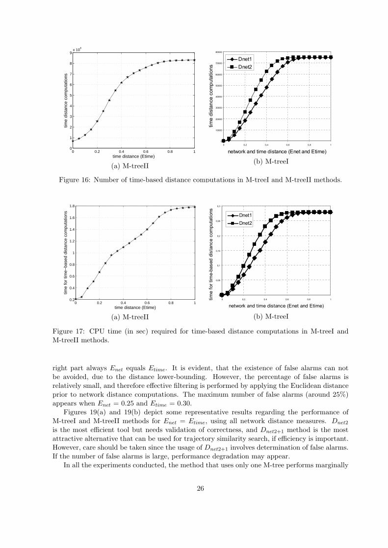
Figure 16 depicts the number of time-based distance computations for M-treeI and M-treeIImethods. We observe that in M-treeII method the number of time-based distance computationsdepends only on the Etime radius, whereas in M-treeI method this value depends on both Enet
and Etime parameters, because in this case the total number of computed distances is equal tothe number of sub-trajectory results returned by the NET-M-tree. Therefore, we expect lesstime-based computations in the M-treeI method than in the M-treeII method. This results inslightly better performance for the M-treeI method regarding time-based distance computationoverhead, as it is illustrated in Figure 17.
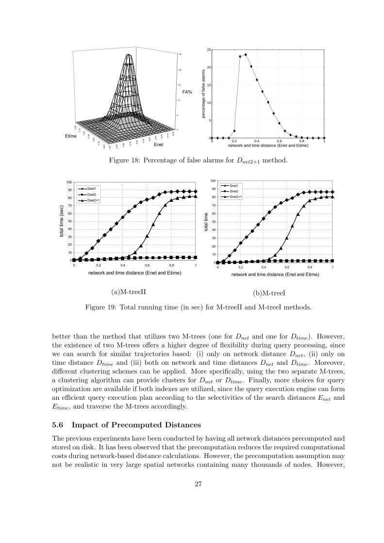
Figure 18 depicts the percentage of false alarms for Dnet2+1, for various values of parametersEnet and Etime. In the left part of the figure, these parameters change freely, whereas in the
25
0 0.2 0.4 0.6 0.8 10
1
2
3
4
5
6
7
8
9x 10
4
time distance (Etime)
time
dist
ance
com
puta
tions
(a) M-treeII
0
10000
20000
30000
40000
50000
60000
70000
80000
0 0,2 0,4 0,6 0,8 1
network and time distance (Enet and Etime)
time distance computations
Dnet1
Dnet2
(b) M-treeI
Figure 16: Number of time-based distance computations in M-treeI and M-treeII methods.
0 0.2 0.4 0.6 0.8 10.2
0.4
0.6
0.8
1
1.2
1.4
1.6
1.8
time distance (Etime)
time
for
time−
base
d di
stan
ce c
ompu
tatio
ns
(a) M-treeII
0
0,05
0,1
0,15
0,2
0,25
0,3
0 0,2 0,4 0,6 0,8 1
network and time distance (Enet and Etime)
time for time-based distance computations
Dnet1
Dnet2
(b) M-treeI
Figure 17: CPU time (in sec) required for time-based distance computations in M-treeI andM-treeII methods.
right part always Enet equals Etime. It is evident, that the existence of false alarms can notbe avoided, due to the distance lower-bounding. However, the percentage of false alarms isrelatively small, and therefore effective filtering is performed by applying the Euclidean distanceprior to network distance computations. The maximum number of false alarms (around 25%)appears when Enet = 0.25 and Etime = 0.30.
Figures 19(a) and 19(b) depict some representative results regarding the performance ofM-treeI and M-treeII methods for Enet = Etime, using all network distance measures. Dnet2
is the most efficient tool but needs validation of correctness, and Dnet2+1 method is the mostattractive alternative that can be used for trajectory similarity search, if efficiency is important.However, care should be taken since the usage of Dnet2+1 involves determination of false alarms.If the number of false alarms is large, performance degradation may appear.
In all the experiments conducted, the method that uses only one M-tree performs marginally
26
0,00
0,10
0,20
0,30
0,40
0,50
0,60
0,70
0,80
0,90
1,00
0,00
0,15
0,30
0,45
0,60
0,75
0,90
0
5
10
15
20
25
FA%
Enet
Etime0 0.2 0.4 0.6 0.8 1
0
5
10
15
20
25
network and time distance (Enet and Etime)
perc
enta
ge o
f fal
se a
larm
s
Figure 18: Percentage of false alarms for Dnet2+1 method.
0
10
20
30
40
50
60
70
80
90
100
0 0,2 0,4 0,6 0,8 1
network and time distance (Enet and Etime)
total time (sec)
Dnet1
Dnet2
Dnet2+1
(a)M-treeII
0
10
20
30
40
50
60
70
80
90
100
0 0,2 0,4 0,6 0,8 1
network and time distance (Enet and Etime)
total time
Dnet1
Dnet2
Dnet2+1
(b)M-treeI
Figure 19: Total running time (in sec) for M-treeII and M-treeI methods.
better than the method that utilizes two M-trees (one for Dnet and one for Dtime). However,the existence of two M-trees offers a higher degree of flexibility during query processing, sincewe can search for similar trajectories based: (i) only on network distance Dnet, (ii) only ontime distance Dtime and (iii) both on network and time distances Dnet and Dtime. Moreover,different clustering schemes can be applied. More specifically, using the two separate M-trees,a clustering algorithm can provide clusters for Dnet or Dtime. Finally, more choices for queryoptimization are available if both indexes are utilized, since the query execution engine can forman efficient query execution plan according to the selectivities of the search distances Enet andEtime, and traverse the M-trees accordingly.
5.6 Impact of Precomputed Distances
The previous experiments have been conducted by having all network distances precomputed andstored on disk. It has been observed that the precomputation reduces the required computationalcosts during network-based distance calculations. However, the precomputation assumption maynot be realistic in very large spatial networks containing many thousands of nodes. However,
27
0
5000
10000
15000
20000
25000
30000
35000
40000
10% 20% 30%
Percentage of precomputed distances
Requests/Hits/Misses
MBFR
MBFH
MBFM
(a) Memory buffer activity
0
5000
10000
15000
20000
25000
30000
35000
10% 20% 30%
Percentage of precomputed distances
Disk Buffer Requests/Hits/Misses
DBFR
DBFH
DBFM
(b) Disk buffer activity
Figure 20: Memory and disk buffer activity for variable disk buffer sizes.
0
100
200
300
400
500
600
700
800
900
1000
1100
0,00 0,05 0,10 0,15 0,20 0,25 0,30 0,35 0,40 0,45
Enet,Etime
Total Time (sec)
Buf-10%
Buf-20%
Buf-30%
(a) M-treeII
0
100
200
300
400
500
600
700
800
900
1000
1100
0,00 0,05 0,10 0,15 0,20 0,25 0,30 0,35 0,40 0,45
Enet,Etime
Total Time (sec)
Buf-10%
Buf-20%
Buf-30%
(b) M-treeI
Figure 21: Total running time for Dnet2+1 for variable query radius and disk buffer sizes.
even for small spatial networks, if the main memory buffer fails to achieve an acceptable hitratio, many distance computations will be invoked, resulting in performance degradation.
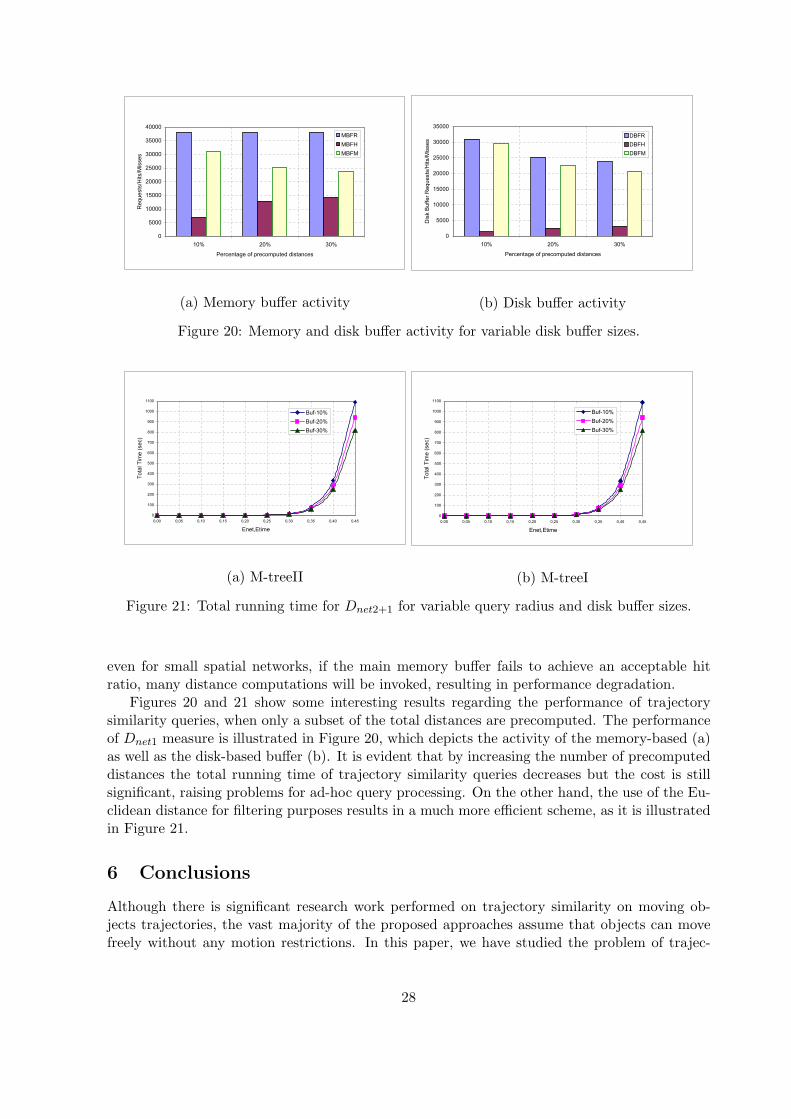
Figures 20 and 21 show some interesting results regarding the performance of trajectorysimilarity queries, when only a subset of the total distances are precomputed. The performanceof Dnet1 measure is illustrated in Figure 20, which depicts the activity of the memory-based (a)as well as the disk-based buffer (b). It is evident that by increasing the number of precomputeddistances the total running time of trajectory similarity queries decreases but the cost is stillsignificant, raising problems for ad-hoc query processing. On the other hand, the use of the Eu-clidean distance for filtering purposes results in a much more efficient scheme, as it is illustratedin Figure 21.
6 Conclusions
Although there is significant research work performed on trajectory similarity on moving ob-jects trajectories, the vast majority of the proposed approaches assume that objects can movefreely without any motion restrictions. In this paper, we have studied the problem of trajec-
28

tory similarity query processing in network-constrained moving objects. We have defined twoconcepts of similarity. The first is based on the network distance and the second is based onthe time characteristics of the trajectories. By using these concepts, we have defined distancemeasures Dnet to capture the network similarity and a distance measure Dtime to capture thetime-based similarity of trajectories. All proposed measures satisfy the metric space properties,and therefore, metric-based access methods can be used for efficient indexing and searching.
To support trajectories of different description lengths, a decomposition process is applied.Each trajectory is split to a number of sub-trajectories, which are then indexed by M-trees.The NET-M-tree is used for the Dnet measure, whereas the TIME-M-tree is used for the Dtime
measure. Two methods have been studied: (i) the M-treeI method, which uses only the NET-M-tree and (ii) the M-treeII method, which utilizes both trees. Performance evaluation results showthat trajectory similarity can be efficiently supported by these schemes. In all the experimentsconducted, the method that uses only one M-tree performs marginally better than the methodwhich utilizes two M-trees. However, the existence of two M-trees offers a higher degree offlexibility during query processing.
Future research may involve: (i) the investigation of alternative indexing schemes, (ii) thestudy of approximate processing and (iii) the efficient support of trajectory-based k-nearest-neighbor processing, and (iv) the utilization of the proposed similarity measures for data mining(e.g., trajectory clustering).
References
[1] T. Brinkhoff: “A Framework for Generating Network-Based Moving Objects”, Geoinfor-matica, Vol6, No.2, pp.153-180, 2002.
[2] P. Ciaccia, M. Patella, P. Zezula: “M-tree: An Efficient Access Method for SimilaritySearch in Metric Spaces”, Proceedings of the 23rd International Conference on Very LargeDatabases (VLDB), 1997.
[3] C. Faloutsos, M. Ranganathan, Y. Manolopoulos: “Fast Subsequence Matching in Time-Series Databases”, Proceedings of the ACM SIGMOD Conference, 1994.
[4] A. Guttman: “R-trees: a dynamic index structure for spatial searching”, Proceedings of theACM SIGMOD Conference, pp.4757, 1984.
[5] J.-R. Hwang, H.-Y. Kang and K.-J. Li: “Spatio-temporal Similarity Analysis BetweenTrajectories on Road Networks”, ER Workshops, pp.280-289, 2005.
[6] J.-R. Hwang, H.-Y. Kang, K.-J. Li: “Searching for Similar Trajectories on Road NetworksUsing Spatio-temporal Similarity”, Proceedings of the 10th East European Conference onAdvances in Databases and Information Systems (ADBIS), pp.282-295, 2006.
[7] C.S. Jensen, J. Kolarvr, T.B. Pedersen, I. Timko: “Nearest Neighbor Queries in Road Net-works”, Proceedings of the 11th ACM International Symposium on Advances in GeographicInformation Systems (ACM GIS), 2003.
[8] G. Kollios, D. Gounopoulos and V.J. Tsotras: “Nearest Neighbor Queries in a Mobile En-vironment”, Proceedings of the International Workshop on Spatio-temporal Database Man-agement, pp.119-134, 1999.
29
[9] G. Kollios, D. Gunopoulos, V. Tsotras: “On Indexing Mobile Objects”, ACM PODS,pp.261-272, 1999.
[10] I. Lazaridis, K. Porkaew, S. Mehrotra: “Dynamic Queries over Mobile Objects”, EDBT,pp.269-286, 2002.
[11] P. Laurinen , P. Siirtola , J. Roning: “Efficient Algorithm for Calculating Similarity Be-tween Trajectories Containing an Increasing Dimension”, Proceedings of the 24th IASTEDInternational Conference on Artificial Intelligence and Applications, pp.392-399, 2006.
[12] S.-L.Lee, S.-J. Chun, D.-H. Kim, J.-H. Lee, C.-W. Chung: “Similarity Search for Multi-dimensional Data Sequences”, Proceedings of the 16th International Conference on DataEngineering (ICDE), 2000.
[13] D. Lomet, B. Salsberg: “Access Methods for Multiversion Data”, ACM SIGMOD, pp.315-324, 1989.
[14] N. Meratnia , R. A. de By: “Aggregation and Comparison of Trajectories”, Proceedings ofthe 10th ACM international symposium on Advances in Geographic Information Systems(ACM GIS), 2002.
[15] M.A. Nascimento, J.R.O. Silva: “Towards Historical R-trees”, ACM SAC, 1998.
[16] D. Papadias, J. Zhang, N. Mamoulis: “Query Processing in Spatial Network Databases”,Proceedings of the 29th International Conference on Very Large Databases (VLDB), 2003.
[17] D. Pfoser, C.S. Jensen, Y. Theodoridis: “Novel Approaches to the Indexing of Mov-ing Object Trajectories”, Proceedings of the 26th International Conference on Very LargeDatabases (VLDB), pp.395-406, 2000.
[18] S. Saltenis, C.S. Jensen, S. Leutenegger, M. Lopez: “Indexing the Positions of ContinuouslyMoving Objects”, ACM SIGMOD, pp.331-342, 2000.
[19] J. Sankaranarayanan, H. Alborzi, H. Samet: “Efficient Query Processing on Spatial Net-works”, Proceedings of the 13th ACM International Symposium on Geographic InformationSystems (ACM GIS), 2005.
[20] Y. Tao, D. Papadias: “Efficient Historical R-trees”, Proceedings of the International Con-ference on Scientific and Statistical Database Management (SSDBM), 2001.
[21] Y. Tao and D. Papadias: “MV3R-tree - a Spatio-Temporal Access Method for Timestampand Interval Queries”, Proceedings of the 27th International Conference on Very LargeDatabases (VLDB, pp.431- 440, 2001.
[22] Y. Theodoridis, T. Sellis, A.N. Papadopoulos and Y. Manolopoulos: “Specifications for Effi-cient Indexing in Spatio-temporal Databases”, Proceedings of the International Conferenceon Scientific and Statistical Database Management (SSDBM), 1998.
[23] C. Traina, A.J.M. Traina, B. Seeger and C. Faloutsos: “Slim-Trees: High PerformanceMetric Trees Minimizing Overlap Between Nodes”, Proceedings of the 7th InternationalConference on Extending Database Technology (EDBT), pp.51-65, 2000.
30

[24] M. Vlachos, D. Gunopulos, G. Kollios: “Robust Similarity Measures for Mobile ObjectTrajectories”, Proceedings of the 5th International Workshop on Mobility in Databases andDistributed Systems, 2002.
[25] M. Vlachos, G. Kollios, D. Gunopulos: “Discovering Similar Multidimensional Trajecto-ries”, Proceedings of the 18th IEEE International Conference on Data Engineering (ICDE),2002.
[26] O. Wolfson, B. Xu, S. Chamberlain, L. Jiang: “Moving Objects Databases: Issues and So-lutions”, Proceedings of the International Conference on Scientific and Statistical DatabaseManagement (SSDBM), pp.111-122, 1998.
[27] O. Wolfson, B. Xu, S. Chamberlain: “Location Prediction and Queries for Tracking MovingObjects”, Proceedings of the 16th IEEE International Conference on Data Engineering(ICDE), pp.687-688, 2000.
[28] Y. Yanagisawa, J.-I. Akahani, T. Satoh: “Shape-Based Similarity Query for Trajectory ofMobile Objects”, Proceedings of the 4th International Conference on Mobile Data Manage-ment (MDM), pp.63-77, 2003.
[29] J.S. Yoo, S. Shekhar: “In-Route Nearest Neighbor Queries”, GeoInformatica, Vol.9, No.2,pp.117-137, 2005.
31