seasonal and annual variability of global winds and …dust.ess.uci.edu/ppr/ppr_arj12.pdfseasonal...

Seasonal and annual variability of global winds and wind

power resources

Journal: Energy & Environmental Science

Manuscript ID: EE-ART-10-2011-002906

Article Type: Paper

Date Submitted by the Author: 14-Oct-2011

Complete List of Authors: archer, cristina; University of Delaware, College of Earth, Ocean, and Environment; California State University Chico, Geological and Environmental Sciences

Energy & Environmental Science

Energy & Environmental Science

Guidelines to Referees

Energy & Environmental Science (EES) — www.rsc.org/ees

EES is a community-spanning journal that bridges energy and the environment. EES publishes insightful science of the highest quality.

July 2011 - the new official EES Impact Factor is announced as 9.45

The journal's scope is intentionally broad, covering all aspects of energy conversion and storage (and their environmental impact), as well as aspects of global atmospheric science, climate change and environmental catalysis.

It is the policy of the Editorial Board to stress an extremely high standard for acceptance

Accepted papers must report insightful, world-class quality science of significant general interest to the journal’s wide readership. We ask referees to examine manuscripts very carefully, and recommend rejection of articles which do not meet our very high novelty, quality and impact expectations. Please state if a paper would be better suited to a more specialised journal. Routine, fragmented or incremental work, however competently researched and reported, should not be recommended for publication. If you rate the article as ‘routine’ yet recommend acceptance, please give specific reasons for this in your report. EES continues to enjoy great success as a journal, attracting much attention and publishing important articles from world-leading research groups. Thank you very much for your assistance in evaluating this manuscript. Your help and guidance as a referee is greatly appreciated. With our best wishes, Professor Nathan Lewis Philip Earis ([email protected]) Editor-in-Chief Managing Editor

General Guidance (For further details, see the RSC’s Refereeing Procedure and Policy)

Referees have the responsibility to treat the manuscript as confidential. Please be aware of our Ethical Guidelines which contain full information on the responsibilities of referees and authors.

When preparing your report, please: • Comment on the originality, importance, impact and scientific reliability of the work; • State clearly whether you would like to see the paper accepted or rejected and give detailed comments (with references, as appropriate) that will both help the Editor to make a decision on the paper and the authors to improve it;

Please inform the Editor if:

• There is a conflict of interest; • There is a significant part of the work which you are not able to referee with confidence; • If the work, or a significant part of the work, has previously been published, including online publication, or if the work represents part of an unduly fragmented investigation.

When submitting your report, please:

• Provide your report rapidly and within the specified deadline, or inform the Editor immediately if you cannot do so. We welcome suggestions of alternative referees.

If you have any questions about reviewing this manuscript, please contact the Editorial Office at [email protected]

Page 1 of 18 Energy & Environmental Science

http://www.rsc.org/ees�

mailto:[email protected]�

http://www.rsc.org/Publishing/ReSourCe/RefereeGuidelines/RefereeingProcedureAndPolicy/index.asp�

http://www.rsc.org/Publishing/ReSourCe/EthicalGuidelines/EthicalGuidelinesandConflictofInterest/sect4.asp�

mailto:[email protected]�

http://www.rsc.org/ees�

Energy and Environmental Science

Cite this: DOI: 10.1039/c0xx00000x

www.rsc.org/xxxxxx

Dynamic Article Links ►

PAPER

This journal is © The Royal Society of Chemistry [year] [journal], [year], [vol], 00–00 | 1

Seasonal and annual variability of global winds and wind power

resources

Cristina L. Archer*a and Mark Z. Jacobson

b

Received (in XXX, XXX) Xth XXXXXXXXX 20XX, Accepted Xth XXXXXXXXX 20XX

DOI: 10.1039/b000000x 5

This paper provides global and regional wind resource estimates obtained with a 3-D numerical model

that dynamically calculates the instantaneous wind power of a modern 5 MW wind turbine at its 100-m

hub height each time step. The model was run at various horizontal resolutions (4x5, 2x2.5, and 1.5x1.5

degrees of latitude and longitude) for several years. Despite differences during the first two years, global

wind power estimates from all runs effectively converged. Global delivered 100-m wind power at high-10

wind locations (≥7 m/s) over land, excluding both polar regions, including transmission, distribution, and

wind farm array losses, but not considering landuse exclusions, is estimated to be 112-120 TW. Seasonal

variations in global wind resources are significant, with 73-89 TW in June-July-August (JJA) versus 159-

167 TW in December-January-February (DJF), with minima in September and maxima in January. The

wind power over land in high-wind locations in the Northern Hemisphere (NH) is ~107 TW, over five 15

times greater than that over the Southern Hemisphere (SH) (~19 TW) on average. The shallow-water

offshore delivered wind power potential (excluding polar regions) is ~9 TW at 100 m, varying between

6.4 and 11.7 TW from JJA to DJF. The theoretical wind power over all land and ocean worldwide at all

wind speeds, considering transmission, distribution, and array losses for typical wind farms, is ~1500

TW. Providing half the world’s energy for all purposes in 2030 from wind would consume <0.5% of the 20

world’s wind power at 100 m, hardly affecting total power in the atmosphere.

1. Introduction

Wind energy is expected to play a major role in the transition

from finite and polluting energy sources - fossil and fissile fuels -

to a clean, sustainable, and perpetual renewable energy 25

infrastructure1. Although it is well known that the global wind

resource is large2,3,4,5,6, the exact magnitude of extractable wind

power available worldwide is still under debate, mainly for four

reasons: 1) the assumptions and definitions used in calculating

global wind power are often inconsistent; 2) wind speed data at 30

the hub height of modern wind turbines (~100 m) are few and

sparse; 3) global model maps evaluated against data are not

available at high resolution, either spatially or temporally; and 4)

the conversion from wind speed to wind power is often calculated

inconsistently because it requires assumptions about specific 35

turbines and their efficiencies as well as transmission and wake

losses.

First, the term “wind power potential” is not unequivocal. It

can refer to one of four different types of potential3, loosely

defined as: 40

- Theoretical potential: the average kinetic energy in the winds at

each instant at all levels in the atmosphere at all points,

regardless of land cover, technology, efficiencies, or cost. As

explained in section 3.2, a better measure of the theoretical

wind power potential may be the added kinetic energy 45

dissipation that does not introduce significant climatic effects.

- Technical potential: the fraction of the theoretical wind power

potential that can be extracted with modern technologies (thus

at hub height, over windy land and windy near-shore

locations only, including limitations due to minimum and 50

maximum wind speeds required to operate a turbine and

array, transmission, and distribution losses).

- Practical potential: the wind power potential excluding areas

with practical restrictions, such as conflicting land and water

uses or remoteness. 55

- Economical potential: the fraction of practical wind power

potential that can be harnessed after economic and financial

considerations are included.

The need for clear, unequivocal definitions of wind power

potentials has been addressed in Hoogwijk et al.3 and in GEA7. 60

Because such consistency in the definitions is still lacking in the

literature, estimates of wind power potential can vary by orders of

magnitude. Since the technical potential is possibly the most

relevant, objective, and insensitive to market fluctuations, it is the

primary focus of this study. 65

Second, the global technical wind power potential is

challenging to evaluate because worldwide wind speed data are

Page 2 of 18Energy & Environmental Science

2 | Journal Name, [year], [vol], 00–00 This journal is © The Royal Society of Chemistry [year]

not available at the hub height of modern wind turbines (~100 m).

As such, interpolation and extrapolations methods over hundreds

of meters of altitude have been proposed, such as the Least

Square Error method4,8 or the log- and power-laws9,10. These

techniques can be applied to both observational data and model 5

results, but are approximate because they are based partly on

theoretical and partly on empirical considerations10. In this study,

this limitation is overcome by using a 3-D atmospheric model

with two layers with centers very close to 100 m, allowing a

nearly precise model estimate of 100-m wind speeds. 10

In addition, global maps of the wind resource at hub height are

not available at spatial and temporal resolutions that are fine

enough to resolve significant local wind features or seasonal and

monthly fluctuations of the global wind resource. Observation-

based estimates, such as Archer and Jacobson4, are limited by the 15

sparse data in most regions of the globe. Fine-resolution maps are

available for certain regions, such as the U.S. West Coast11,12, but

not for the entire globe, due to practical computational

limitations. No study to date has addressed the seasonal and

monthly fluctuations of wind power at the global scale. This 20

study will address both issues – spatial and temporal resolution -

by providing coarse, medium, and fine resolution maps of global

wind power, season by season and month by month. A limitation

of this study is that sub-grid scale topography could not be

properly simulated at the resolutions modeled here. However, the 25

model did treat subgrid soil and land use classes and calculated

surface energy and moisture fluxes over each subgrid soil class

every time step in the model. Running global simulations at

higher-resolution than was done here was not possible given the

computational resources available for this study. 30

Finally, the inconsistent methods of converting from wind

speed to wind power is another reason for differences in wind

power estimates in the literature. Previous model-based wind

power mapping efforts estimated wind resources using

information averaged over time from offline meteorological 35

simulations, either by calculating the theoretical power available

in the wind every 6 or 12 hours13,14, applying a power curve to

offline reanalyses of wind speeds every 6 hours15, or using fitting

equations to calculate the capacity factor from wind speeds

averaged over one year11. In this paper, wind power distributions 40

were obtained by using the wind power curve of a selected wind

turbine, the 5-MW model by REPower

(http://www.repower.de/fileadmin/download/produkte/RE_PP_5

M_uk.pdf), directly in the meteorological model to calculate

instantaneous power from instantaneous wind speed each model 45

time step of 30 s in all simulations.

2. Methods

2.1 Implementation of a wind turbine power curve into the model

The model used for this study was GATOR-GCMOM, a one-50

way-nested (feeding information from coarser to finer domains)

global-regional Gas, Aerosol, Transport, Radiation, General

Circulation, Mesoscale, and Ocean Model that simulates climate,

weather, and air pollution on all scales and has been evaluated

extensively16,17,18. In this paper, we further compare ocean wind 55

speed data from the model with satellite data. The processes

within the model have also been compared with those of other

coupled climate-air pollution models in Zhang19.

For this study, only the global domain was used, but at three

horizontal resolutions. The model treated 47 vertical layers up to 60

60 km in each simulation, including 15 layers in the bottom 1 km.

The four lowest levels were centered at approximately 15, 45, 75,

and 106 m above the ground, but the heights of such centers

changed continuously in a small range since the vertical

coordinate system used was the sigma-pressure coordinate. Each 65

time step, though, all wind speeds were interpolated vertically

between two layer centers to exactly 100 m, the hub height of the

wind turbine assumed for the calculations here.

The model solves the momentum equation with the potential-

enstrophy-, vorticity-, energy-, and mass-conserving scheme of 70

Arakawa and Lamb20. Two-dimensional ocean mixed-layer

dynamics conserves the same four properties while predicting

mixed-layer velocities, heights, and energy transport21. The

model solves 3-D ocean energy and chemistry diffusion, 3-D

ocean equilibrium chemistry, and ocean-atmosphere exchange. 75

The model also treats subgrid soil classes, each with a 10-layer

soil model, and surface energy and moisture fluxes separately

over each subgrid class16.

In order to calculate wind power from the model, we first

selected a turbine, the REPower 5M wind turbine. With a 80

diameter of 126 m and a hub height of 100 m, it reaches the rated

power 5 MW at the rated speed of Vrated=12.5 m/s. Manufacturer

power output data as a function of wind speed were provided

only as a graphic curve in one-unit intervals. A third-order

polynomial fit was used to obtain wind power output P as a 85

continuous function of 100-m wind speed v:

P = av3 + bv

2 +cv+ d , (1)

where the coefficients a, b, c, and d are shown in Fig. 1. No

power can be produced at wind speeds lower than 3.5 m/s (cut-in

speed) or higher than 25 m/s (cut-off speed). Because of the 90

change in the curve concavity, different coefficients were derived

for low versus high wind speeds.

Fig. 1 Power curve of the REPower 5M wind turbine, with coefficients

valid below 10 m/s (lower polynomial, black line) and above or equal to 95

10 m/s (upper polynomial, grey line) used to interpolate the

manufacturer’s data.

The dynamical time step in the model was 30 seconds for all

model resolutions simulated. Each dynamical time step, the wind

speed at 100 m above ground level at the horizontal center of 100


This journal is © The Royal Society of Chemistry [year] Journal Name, [year], [vol], 00–00 | 3

each column in the model was applied to Equation 1 to determine

the instantaneous wind power at 100 m for a single wind turbine.

Wind power at 100 m was stored so that monthly, seasonal, and

annual statistics could be obtained.

2.2 Numerical simulations 5

Three simulations were run, each with a different horizontal

resolution and start date (Table 1). Initial conditions for each

simulation were obtained with 1ox1o reanalysis fields22. To

eliminate the effect of the initial state, the model results for the

first several months of each simulation were discarded and only 10

results since March 2007 were retained.

Table 1 Details of the various simulations.

Run

name

Horizontal

resolution

(degrees)

Time step

(s)

Starting date End date

4x5 4 x 5 30 1 Jan 2006 31 Dec 2009

2x2.5 2 x 2.5 30 27 Aug 2005 31 Dec 2009

1.5x1.5 1.5 x 1.5 30 19 Feb 2006 31 Dec 2008

2.3 Assumptions for global wind power calculations

After each simulation, a maximum number of turbines in each

grid cell was determined by dividing the grid cell surface area by 15

the spacing area of a single turbine, estimated as A=7D x 4D,

where D is the turbine diameter (126 m in this case) [Masters23, p.

352]. The power output from the model per turbine for either a

month, season, or year was then multiplied by the number of

turbines in the grid cell to obtain the power available in the cell 20

before the system efficiency was accounted for. This power is

referred to as “turbine power” and is used in this paper only for

calculations of the capacity factor (in Section 3.1). Power output

accounting for system efficiency was then tabulated. This power

is referred to as “end-use power”. Except for capacity factor, all 25

power results reported in this paper are end-use power, thus

accounting for system efficiency.

The system efficiency of a wind farm ηt is the ratio of energy

delivered to raw energy produced by the turbines. It accounts for

array, transmission, and distribution losses (but not for 30

maintenance or availability losses).

Array losses are energy losses resulting from reductions in

wind speed that occur in a large wind farm when upstream

turbines extract energy from the wind, reducing the wind speed

for downstream turbines. Upstream turbines also create vortices 35

or ripples (turbulence) in their wakes that can interfere with

downwind turbines. The greater the spacing between wind

turbines, the lower the array losses due to loss of energy in the

wind, vortices, and wakes. Array losses are generally 5-20

percent23,24. 40

Transmission and distribution losses are losses that occur

between the power source and end users of electricity.

Transmission losses are losses of energy that occur along a

transmission line due to resistance. Distribution losses occur due

to step-up transformers, which increase voltage from an energy 45

source to a high-voltage transmission line and decrease voltage

from the high-voltage transmission line to the local distribution

line. The average transmission plus distribution losses in the U.S.

in 2007 were 6.5 percent25.

The overall system efficiency of a wind farm, accounting for 50

array, transmission, and distribution losses typically ranges from

0.85 to 0.9; here we assumed an average ηt=0.875, corresponding

to a system loss of 12.5 percent.

3. Results

3.1 Mapping the global wind resource at various 55

resolutions

Fig. 2 provides global wind speeds from the three simulations

during the northern hemisphere (NH) winter. Additional maps for

the entire simulation period are available at

http://suntans.stanford.edu/~lozej/mark_model. The strongest 60

winds are in the NH, especially over the waters in the northern

Pacific and Atlantic oceans, where the Aleutian and the Icelandic

low-pressure systems cause storms and strong winds near the

surface. Whereas all runs are consistent with each other in the

NH, some differences are found in the SH. For example, the 65

annular structure of strong winds over the Southern Ocean

appears continuous at 2x2.5 degrees, but somewhat discontinuous

at 1.5x1.5 degrees. Also, a secondary wind speed maximum

appears to the west of northern Australia in the 1.5x1.5 run only.

Overall, however, the runs are in agreement with each other 70

during DJF, although the 2x2.5 run shows generally higher wind

speeds in the SH than does the 1.5x1.5 run.

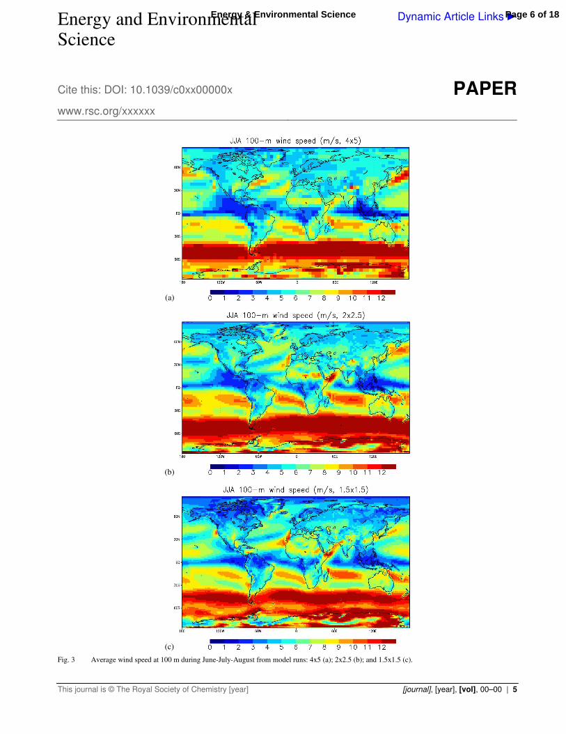
Fig. 3 shows the 100-m wind speed distribution during the NH

summer (JJA). The runs are in good qualitative agreement, with

the 2x2.5 again producing slightly higher and more continuous 75

winds over the Southern Ocean. The localized wind speed

maximum offshore of California is a persistent feature in the

northern Pacific during the NH summer13,11,12 and it represents

possibly the greatest summertime offshore wind resource in

North America during the season with the highest electric load. 80

Although there is a second maximum offshore of Japan in JJA,

the summer wind speed maximum offshore of California is

predicted correctly by this model at all resolutions, with the least

accuracy at 4x5 degree resolution.

85




www.rsc.org/xxxxxx


PAPER


(a)

(b)

(c)

Fig. 2 Average wind speed at 100 m during December-January-February from model runs: 4x5 (a); 2x2.5 (b); and 1.5x1.5 (c).




www.rsc.org/xxxxxx


PAPER


(a)

(b)

(c)

Fig. 3 Average wind speed at 100 m during June-July-August from model runs: 4x5 (a); 2x2.5 (b); and 1.5x1.5 (c).




www.rsc.org/xxxxxx


PAPER


The capacity factor (CF) of a turbine is the ratio of the actual

power generated by the turbine to its rated power. The capacity

factor in this definition does not account for the system

efficiency, only the turbine efficiency and the variability of the

wind, thus is a gross CF. Modern wind turbines installed in areas 5

with average 100-m wind speeds greater than 7 m/s can achieve a

gross CF>40%. By contrast, wind turbines exposed to average

wind speeds lower than 7 m/s are less likely to be economically

feasible26, although recent progress in the development of low

wind speed turbines may reduce this threshold from 7 to 6.5 m/s 10

in the near future. The rest of this analysis focuses on “windy”

areas, defined as those with yearly-average wind speeds at 100 m

≥7 m/s.

Fig. 4 shows the average gross capacity factor in January 2008

obtained with the REPower 5M wind turbine for all grid points 15

over windy land and windy shallow (≤200 m) waters only,

without considering land or water use restrictions. The figure was

obtained by masking out wind speeds lower than 7 m/s and then

overlapping the resulting map with wind power divided by the

rated power of the benchmark turbine (5000 kW). Areas with 20

high CF (>0.3) in Fig. 4 are the most economical for wind power

development over land. Aside from the mid-latitude areas in both

NH continents, noticeable is the vast area in the Sahara and Sahel

deserts with a CF~0.5.

As mentioned in the introduction, the horizontal resolution of 25

these simulations is not fine enough to properly resolve some

meso- and fine-scale features, such as steep topography or sudden

surface roughness or landuse horizontal variations, which can

cause localized high winds. This somewhat coarse resolution,

however, is likely to result in an under-estimate, rather than an 30

over-estimate, of wind speeds and wind power. For example, Fig.

4 shows little potential in Spain and Portugal, whereas both

countries have installed over 30 GW of wind capacity in 2010

alone [need ref].

3.2 The global wind power potential: top-down methods 35

The global wind power potential can be estimated in at least three

ways: from theoretical calculations, from observations, and from

numerical modeling. The first is a top-down approach, the others

are bottom-up.

40

Theoretical calculations rely on the basic equations of motion in

the atmosphere, but require the use of simplifying assumptions

(e.g., hydrostatic equilibrium, quasi-geostrophic balance,

horizontal homogeneity) and spatially- and temporally-averaged

values of physical variables (e.g., albedo, latent heat release, solar 45

radiation, surface roughness) to solve them. Because of these

limitations, the order of magnitude of these estimates, not their

exact values, should be considered valid at most.

A distinction must first be made between the kinetic energy of

the atmosphere (KE), measured either in units of joules (J, for the 50

entire Earth) or J/m2 (joules per square meter of Earth’s surface),

and the so-called KE dissipation rate D expressed either in units

of power (W) or power per unit area (W/m2), which represents

the rate at which kinetic energy naturally drains out of the

atmospheric motion field due to molecular viscous (or frictional) 55

processes, occurring both in the mean flow (~9.5%) and in the

unresolved scales from turbulent stresses (~90.5%)27.



Fig. 4 Average wind turbine capacity factor in all seasons during 2007-2008 over land and offshore locations with yearly-average 100-m wind speed

>7 m/s (excluding both Polar regions) using the REPower 5 MW wind turbine from run 1.5x1.5. The turbine capacity factor shown does not account for

system efficiency losses, which are ~10-15%.

An expression for D is obtained by taking the scalar product of 5

the momentum equation with the velocity vector rv , then

integrating over the entire volume of the atmosphere V with

density ρ:

(2)

where rF is friction per unit mass in m/s2 [Holt28, p. 340], which 10

is expressed as ν∇2rv (or ν

∂2ui

∂x j

2 with the Einstein notation) for

incompressible flows, and ν is the air kinematic viscosity in m2/s.

Note that the volume integral in Eq. (2) can be calculated over

smaller volumes than the entire atmosphere, such as over a region

or in the wake of a turbine. When mechanical or thermal 15



turbulence is considered, then D is the sum of a mean ( ) and a

perturbation (D’) component as follows:

(3)

(4)

where ui indicates a mean and ′u

i a turbulent component of the 5

velocity vector and the bar indicates a time or an ensemble

average [Holt28, p. 340; Peixoto and Oort27, p. 376-377; AMS29].

Dividing Eqs. 2-4 by the Earth’s surface area gives D in units of

W/m2. Note that the term “dissipation rate” often refers to the

expressions inside the integral in Eq. 4 (without the air density) as 10

follows:

ε =ν∂ ′ui

∂x j

2

(5)

which has units of m2/s3 [AMS, 2000] and is always

parameterized in models.

Regardless of the formulation used, the KE dissipation rate D 15

is not a good proxy for wind speed or wind power because it is

either the product of wind speed and friction (Eq. 2 and 3) or the

square of turbulent stresses (Eq. 4). As such, knowing D alone is

not sufficient to reconstruct wind speed.

Whereas the atmosphere has a large reservoir of KE (~11.8 x 20

105 J/m2, Peixoto and Oort27, p. 385), the dissipative term D is

often negligible, except near the Earth’s surface, in regions of

strong wind shear (e.g., the jet streams and in convective clouds)

and of breaking gravity waves; it is also responsible for ocean

surface currents. Because the friction vector always points 25

opposite from the velocity vector, D is always negative (from Eq.

2) and therefore represents a sink, never a source, of KE.

Dissipation D ultimately converts KE to internal energy (IE) via

heating [Lorenz30, p.14]. Part of internal energy itself converts

back to potential energy (PE) through, for example, buoyant 30

convection, and gradients of PE reproduce KE. Treating energy

exchange in the atmosphere involves treating not only PE, KE,

and IE, but also solar and infrared radiation, latent heat,

conduction, and geothermal heat.

The ratio of natural KE dissipation D to the globally- and 35

annually-averaged downward solar radiation at the top of the

atmosphere (~350 W/m2) is the atmospheric efficiency30 η. This

efficiency represents the fraction of the incoming energy that is

fed into the atmosphere to maintain the global circulation against

dissipation. Lorenz30 estimated that η is at most 2% and thus D is 40

~7 W/m2 or 3600 TW for the whole Earth (assuming a surface

area of 5.12 x 1014 m2). King Hubbert31 later estimated a value of

D that was 10x lower: ~370 TW (~0.72 W/m2,) or η ~0.2%.

Subsequent studies indicated that this value was too low. Peixoto

and Oort27,32,33 estimated D ~1.88-2 W/m2, corresponding to 45

~962-1024 TW; Li et al.34 calculated D ~2.06-2.55 W/m2 from

global reanalyses (~1054-1306 TW); and Stacey and Davis35 used

the length of day variations to obtain an estimate for D of 434 TW

(~0.85 W/m2). Sorensen36 [p. 86] states that the few available

direct estimates of dissipation are 4-10 W/m2 (2000-5100 TW), 50

much higher than previous estimates, which are derived indirectly

to ensure consistency with estimates of sources of energy,

suggesting the dissipation is tuned, not calculated from first

principles. In summary, the literature indicates that even the order

of magnitude of dissipation is unclear, with possible values in the 55

450-3800 TW range.

Regardless of its exact value, the KE dissipation rate D is

relevant to wind energy because wind turbines locally increase

atmospheric KE dissipation D by increasing surface friction,

turbulent kinetic energy (TKE) dissipation, and direct conversion 60

to heat. First, just like any mountain, tree, building, or obstacle in

the path of wind, wind turbines increase surface roughness and

therefore increase via increased surface friction. Second,

some KE is converted to turbulent KE (TKE) in the wake (thus

increasing the TKE production term ′ui′u j

∂ui

∂x j

) and then some of 65

this TKE is converted to heat via molecular viscous effects (thus

increasing D’). Third, wind turbines also have another unique

dissipative effect: they force the atmosphere to perform work

(rotating the blades) to generate electricity and thus directly

remove KE from the wind flow (decreasing the wind speed). 70

Since electricity cannot be stored and is almost immediately

converted to heat added back to the atmosphere by end users

dispersed widely, wind turbines result in heat addition back to the

atmosphere over a larger area than a building or tree. The relative

magnitudes of these three effects are currently not known 75

precisely, but some initial parameterizations have been

proposed37.

The third effect, KE conversion to electricity, is at most equal

to 16/27 of the impinging KE (at the Betz limit). The remaining

KE (at least 11/27) is in part converted to TKE (as described 80

above) and in part remains in the mean flow since the mean wind

speed past a wind turbine is reduced but not zero. The exact

distribution of the remaining KE between mean flow and

turbulent wake past the turbine is not known, nor is the fraction

of TKE in the wake that is actually dissipated to heat via 85

molecular viscous processes. In summary, wind turbines can be

considered as converters of atmospheric KE to IE, some of which

is converted back to PE.

Whereas it is accepted that wind turbines increase KE

dissipation locally, the effect of wind turbines on the overall KE 90

dissipation of the atmosphere is yet to be understood. Several

studies suggest that the atmosphere will maintain its current

dissipation rate regardless of the number of obstacles, whether

buildings or wind turbines, that are added at the surface38,39,40,41.

The theoretical justification for this view is that the efficiency of 95

the atmosphere as a heat engine is already nearly maximized and

therefore no additional work can be performed by the atmosphere

given its IE (or thermal) inputs and outputs. This implies that, if

KE dissipation is increased at one location by adding a wind

turbine, KE dissipation must decrease equally somewhere else to 100

keep total dissipation constant. The only way to decrease KE

dissipation away from the turbine is to decrease wind speeds,

which was argued to occur not only in the wake but also at other

locations with simplified numerical simulations40,41. With this

approach, the natural KE dissipation rate D would represent the 105



maximum theoretical limit to wind power extraction.

There are several inconsistencies with this view. First, if KE

dissipation and the thermal inputs and outputs of the atmosphere

remain constant, KE should also stay constant, whereas the

addition of wind turbines decreases KE and local wind speeds. 5

Second, KE cannot decrease without IE increasing (and vice

versa), but this conversion is not possible without increasing KE-

to-IE conversion (or decreasing IE-to-KE conversions), which

cannot happen if D is constant. Third, if 100% of the KE

dissipation were “extracted” via wind turbines, then the near-10

surface wind speeds would be zero everywhere except where the

turbines are. Instead, Young et al.42 found that observed near-

surface wind speeds have been increasing, not decreasing, over

the oceans during the past 20 years despite the addition of dozens

of gigawatts of installed wind power worldwide. These 15

inconsistencies suggest that another explanation is needed.

Other studies cite potential climate effects of extracting wind

energy. For example, Miller et al.41 claim that the climate effects

of extracting 18-68 TW of wind power are equivalent to doubling

carbon dioxide. However, their study first ignores the fact that 20

wind power results in no net additional heat to the air since it

replaces thermal power plants (coal, nuclear, natural gas), all of

which directly add the same or more heat to the air than wind

power directly through combustion or nuclear reaction. These

other sources, including nuclear, also add carbon dioxide during 25

the processing or use of their fuel, which wind energy does not

do. Second, even if wind turbines did not replace thermal power

plants, the actual heat resulting from converting 18-68 TW of

wind power to electricity, which then gets converted to heat, is

0.035�0.13 W/m2. The radiative heating due to doubling of CO2 30

is 3.7 W/m2, a factor of 28-106 higher. As such, even if 18-68

TW of wind power were extracted, it would affect temperatures

by 28-106 times less than doubling carbon dioxide, not by the

same amount. However, since wind displaces thermal power

plants, its net heat added to the atmosphere is effectively zero. 35

We propose here that KE dissipation is not constant for the

Earth. Any increase in the number of obstacles increases

dissipation, and any increase in KE dissipation causes an equal

increase in IE generation rate (via heat) and therefore a change in

the energy balance, but an overall conservation of energy. This is 40

consistent with KE dissipation being a transfer of energy from the

KE to the IE reservoir30. To compensate for this additional IE

generation, the atmosphere must therefore increase the transfer of

a portion of energy from the IE back to the KE reservoir, via an

increase in the Potential Energy (PE) generation first and then an 45

increase in the PE-to-KE conversion via adiabatic processes. At

equilibrium, this KE generation must offset KE dissipation43. KE

decreases initially when turbines are installed and the KE

dissipation rate is increased (output > input), consistent with

findings by Santa Maria and Jacobson44. At equilibrium, 50

however, this lower KE is maintained (output = input), and so is

the higher IE. As such, altering KE dissipation can feed back to

the Earth’s climate, albeit by an uncertain quantity. However, we

do know that the building of all cities and infrastructure for

human civilization to date have had little effect on global climate 55

through the change in the KE dissipation rate relative to changes

in evapotranspiration, albedo, and specific heat (e.g., the urban

heat island effect) and changes in precipitation due to urban areas.

If this proposed theory is correct, then is there an upper limit to

the human extraction rate of kinetic energy via wind turbines 60

such that significant impacts on the global circulation would not

occur? This value would be the limit to wind power extraction.

Archer and Caldeira14 showed with a modified climate model

(inclusive of KE dissipation to heat by idealized airborne wind

turbines scattered uniformly in the entire atmosphere) that, for 65

KE extraction of the same order of magnitude as human energy

consumption in 2005 (~18 TW, ~1% of natural D), climatic

effects are negligible; however, for KE extractions of 840 and

2010 TW (50 times and 100 times the current human energy

consumption, respectively, or 50% and 100% of natural D), 70

larger, non-linear changes to the climate can occur, such as cooler

surface temperatures and increased polar sea ice extent. Thus,

their findings support indirectly that an upper limit to additional

dissipation from wind turbines lies between 1% and 50% of the

current D. 75

Regardless of the actual maximum value of KE dissipation,

even if all human demand for energy were met with wind power,

the current KE dissipation would only be increased by ~1%, with

negligible climatic effects14. Also, because wind generation

would replace other larger sources of heat such as coal, natural 80

gas, or nuclear power plants, which were not accounted for by

Archer and Caldeira14, the net heat input is expected to be even

smaller and thus the climatic impact reduced43.

As discussed, the order of magnitude of the natural dissipation

rate of kinetic energy by winds is still under debate, with 85

estimates ranging from 450 to 3800 TW. Using 1200 TW as an

intermediate (~2.2 W/m2) and 10% as a intermediate between 1%

and 50% for the maximum additional KE dissipation by wind

turbines, an estimate of the theoretical maximum wind power

extractable with little climate impact is 0.10 x 1200 TW = 120 90

TW.

World end-use power demand in 2008 for all purposes was

approximately 12.5 TW and is expected to grow to 16.9 TW by

2030. Electrification and conversion to electrolytic hydrogen of

the transportation, energy, and industrial sectors would reduce 95

2030 end-use power demand to 11.5 TW1. Jacobson and

DeLucchi1 suggested a feasible target of 50 percent (5.75 TW) of

this power supplied by wind. Thus, if half the world’s power for

all purposes were to be supplied by wind, and assuming previous

literature estimates of world wind resources, only 0.1-1% of the 100

world’s all-wind-speed wind power at 100 m would be needed,

with negligible climatic impacts. In other words, the world wind

resource is 100-1000 times what the world needs in terms of wind

power.

3.3 The global wind power potential: bottom-up 105

methods

Whereas theoretical calculations represent a top-down approach

to the evaluation of the global wind power potential, observation-

and model-based estimates are bottom-up approaches in which

the total potential is determined from the combined output of 110

individual wind turbines scattered over the Earth.

All bottom-up methods share one common implicit

assumption: each additional wind turbine alters the atmospheric

circulation only within the wake volume downwind of the

turbine. Within this volume, wind speeds first decrease then 115

increase, eventually converging to the background wind speed.



As wind speeds first decrease within a wake, the vertical gradient

in wind speed increases, increasing the downward turbulent flux

of faster winds from aloft to hub height and decreasing the

downward turbulent flux of winds at hub height to the surface,

ultimately replenishing winds some distance downwind of each 5

turbine. Similarly, the horizontal pressure gradient force

continuously acts on the winds at a given height and contributes

to regenerating winds. Whether full regeneration in the wake

occurs depends on the distance between turbines in the direction

of the wind and on the pressure gradient force and the rate of 10

turbulent diffusion. In wind turbine arrays, additional interactions

between wakes can occur24, 45.

Fig. 5 shows evidence of wind regeneration in an array. The

data, from Frandsen24, indicate that, despite wind speed

reductions and incomplete regeneration past turbine rows 1 and 2, 15

wind speeds in subsequent turbine rows stayed constant or

increased compared with row 3. This could occur only with the

regeneration mechanisms discussed. The overall reduction in

wind speed between rows 1 and 7 is only ~8% with diameter

spacing of 6D between rows. This represents an array efficiency 20

of 92%. Similarly, Barthelmie et al.45 found that, after an initial

decrease in wind power output between the first and the second

row at two large offshore wind farms in Denmark, wind power

output in subsequent rows either stayed constant or slightly

increased. Greater spacing results in greater array efficiency [e.g., 25

Masters23].

Fig. 5 Measured ratio of wind speed at the given turbine row to that

at the first turbine row from Norrekoer Enge II wind farm for four cases

of initial upstream wind speed U (m/s). Wind speeds were derived from 30

power output from an average of six 300-kW turbines in each of seven

rows spaced 7D to 8D within rows and 6D between rows. The solid line is

the result of a wake model. Reproduced with permission from Frandsen24.

Fig. 5 and results from similar studies provide support for the

contention that turbine energy lost in a wake volume substantially 35

regenerate by the end of the wake for remaining turbines.

However, energy lost within the wake volume does reduce the

instantaneous total kinetic energy in the atmosphere. Santa Maria

and Jacobson44 quantified the net reduction in the globally-

averaged kinetic energy in the boundary layer due to wake-40

volume losses if the entire world’s energy supply were powered

by wind and found the total loss to be small. Their study did not

account for the conversion of electrical energy back to heat then

potential energy then kinetic energy again, which would make the

losses smaller, nor did it calculate the actual wake volumes, 45

which could be larger or smaller than assumed. Nevertheless,

even a factor of 100 underestimate of energy loss would not

change the conclusion that powering the entire world with wind

would not reduce beyond 1 percent the energy in the atmosphere.

This result justifies the use of the bottom-up method of summing 50

power output from individual wind farms to determine global

wind power potential.

Archer and Jacobson4 used a network of 446 sounding and

7753 surface stations to calculate the technical wind power

potential at 80 m above the ground over land and near-shore from 55

observations as ~72 TW. They estimated that ~13% of the global

land (excluding Antarctica but including near-shore ocean areas)

could be covered with wind turbines, with no landuse restrictions,

to extract this power. A spacing of 7D x 4D (D is the diameter of

the swept area, or twice the blade length) between 1.5 MW wind 60

turbines was assumed23 to account for the loss and regeneration

of winds in the wake volume downwind of each turbine. If 20-

40% of 72 TW could be extracted after landuse and other

restrictions were accounted for, the resulting practical wind

power from Archer and Jacobson4 would be 0.2-0.4 x 72 TW = 65

14.4-28.8 TW, much more than needed to power the world’s

energy for all purposes in 2030.

Hoogwijk et al.3 used the bottom-up method too with surface

observed wind speed data (interpolated onto a 0.5x0.5 degree

grid) and several landuse, altitude, and wind regime constraints to 70

estimate that 96 PWh could be extracted from winds at 69 m each

year over land (or ~11 TW) via turbines. This estimate of the

practical wind power potential is lower than the 14-28 TW

derived above from Archer and Jacobson4 due to their use of

empirical profiles rather than actual sounding data to provide 75

vertical profiles, their use of a lower hub height (69 vs. 80 m),

and lower density of wind turbines (4 vs. 9 MW/km2).

Wind observations can also be derived from satellite products.

For example, wind speeds derived from space-based

scatterometer on QuikSCAT (at 12.5 km horizontal resolution) 80

were used by Li et al.34 to evaluate the wind power distribution

over the ocean. However, no global wind power output at near-

shore locations were provided. Capps and Zender46 utilized 7

years of QuikSCAT 10-m wind speed data over the oceans (at

0.25ox0.25o horizontal resolution) and extrapolated them to 100 85

m using Monin-Obukhov similarity theory. With high-resolution

bathymetry data (one arc-minute), they calculated that up to 39

TW of wind power are available at shallow (≤ 200 m) offshore

locations worldwide, without including water-use restrictions.

Lu et al.5 used a new reanalysis dataset, the Goddard Earth 90

Observing System Data Assimilation System version 5 (GEOS-

5), at a horizontal resolution of 2/3º longitude by 1/2º latitude and

a time resolution of 6 hr, with 2.5 MW wind turbines over land

(excluding forested, urban, permanently ice covered, and inland

water regions) and 3.6 MW turbines deployed offshore 95

(excluding depths >200 m and distances from shore >93 km),

both with 100-m hub heights, to estimate the global technical

wind power potential as ~840 PWh, or 96 TW, over land and

near-shore areas with capacity factor greater than 20% and

accounting for exclusions over forested land and some other 100

types of land use. Without limiting the capacity factor, their

practical global potential (on- and off-shore) was 1300 PWh, or

148 TW. Because the GEOS-5 reanalyses include both model



results (for meteorological fields, not wind power output) and

observations, this is both a model- and observation-based

estimate.

3.4 Seasonality and geographic distribution of the global wind power potential 5

Globally-integrated wind power is calculated here with a bottom-

up approach by summing the area-weighted hourly wind power in

all grid cells over land (excluding regions poleward of 66.56

degrees North and 60 South) that exhibited a yearly-average wind

speed at 100 m above ground greater than 7 m/s. The turbine 10

density is 106 m2/(7Dx4D)23,16 = 2.25 turbines/km2, where D is

the diameter of the REPower 5M turbine (126 m). This

corresponds to an installed capacity density of 11.25 MW/km2.

Wind turbines are assumed to affect circulation in their wake

volumes only, thus interactions among wakes are neglected. The 15

monthly totals for the three runs 4x5, 2x2.5, and 1.5x1.5 for the

later years of the simulations are shown in Fig. 6.

Fig. 6 Globally-integrated monthly wind power at 100 m above

ground over land (excluding polar regions and including system losses) in 20

locations where the mean wind speed exceeds 7 m/s for the three

simulations: 4x5, 2x2.5, and 1.5x1.5.

The results are quite remarkable. First, the three runs give very

similar results, generally varying within ±14.5% from one

another. As expected, the coarse-resolution run (4x4.5) gives 25

slightly lower wind power than both the intermediate (2x2.5) and

the fine (1.5x1.5) resolution runs (-6% and -5% respectively),

which are very similar to one another (~6% difference on

average). Because of this similarity, the fine-resolution run was

stopped in December 2008, due to its high computer time and 30

storage requirements. As such, the intermediate-resolution run

(2x2.5) will be used as the benchmark for further analyses in the

rest of this paper.

Second, wind energy at the global scale is neither constant

throughout the seasons, as one might expect from the 35

complementarity of the seasons in the two hemispheres, nor bi-

modal, as the generally-stronger winter winds in both

hemispheres might suggest. The monthly pattern of wind power

over land is dominated by the seasons in the Northern

Hemisphere (NH), with maxima in DJF and minima in 40

September. Global wind power over land during the NH winter

(DJF) is ~2x greater than that during the NH summer (JJA),

consistent with the higher intensity of the NH energy cycle in

January than in July observed by Oort and Peixoto32 [p. 2715].

Furthermore, Fig. 7 shows that wind power over land in the 45

NH (114 TW on average, dark green shade) is about 2x greater

than that in the SH (60 TW on average, light green shade) on

average, and up to 7x during the NH winter, even when

Antarctica is included in the SH land. This can be explained by

the difference in the land areas of the two hemispheres, because 50

the land area in the NH is ~2.5x the land area in the SH. If both

polar regions are excluded, then the ratio of wind power over

windy land in the NH to that in the SH is >5 on average (107 vs.

19 TW), reaching >10 in December (185 vs. 17 TW). This is

because the area of windy land in the NH is ~5 times larger than 55

that in the SH (30,632,880 vs. 6,704,187 km2) if the polar regions

are excluded.

Fig. 7 Stacked-area plot of total wind power from areas with yearly-60

average wind speed >7 m/s over land and over ocean in the Northern and

Southern hemispheres (NH and SH respectively), including the polar

regions and including system losses. Total wind power from all areas with

monthly-average wind speed >0 m/s is shown with a black solid line. The

total wind power over ocean is purely hypothetical and is only shown for 65

comparison purposes.

Further insights into the wind power resources over land in the

two hemispheres can be provided by area-averaged wind speeds.

Fig. 8 shows that area-averaged monthly 100-m wind speeds over

land (excluding regions poleward of 60 degrees North and South) 70

are higher in the NH (6.25 m/s) than in the SH (5.40 m/s). The

opposite is true over the oceans (at all latitudes), where winds

speeds are higher in the SH (8.79 m/s) than in the NH (6.53 m/s).

This suggests that the two hemispheres have different wind

resources. The SH is generally more energetic (average wind 75

speed is 7.91 m/s in the SH and 6.35 m/s in the NH) and its

seasonal cycles are driven by the oceans. The latter is due to the

large fraction of SH covered by oceans (78%), and the former is

due to a combination of two factors: first, the lower surface

roughness of the ocean compared to that of land, and, second, the 80

absence of any land barrier to the westerly winds around

Antarctica causes the highest wind speeds on the planet to be

observed in the Southern Ocean. On the other hand, 60% of the

NH is covered by land, thus it is generally less energetic than the

SH, but its wind speed over land is higher than in the SH. 85



Fig. 8 Area-averaged 100-m wind speed from run 2x2.5 over land

(excluding polar regions) and over oceans in each hemisphere and

globally.

In order to put the wind power estimates over land in context, 5

Fig. 7 also shows the wind power over the oceans in both

hemispheres from run 2x2.5, calculated with the same wind

power curve used over land (Fig. 1) at grid cells with monthly-

average wind speeds ≥7 m/s. These ocean totals are hypothetical

and do not represent a feasible near-term potential due to the 10

great distance from shore of most locations and the current

difficulty of installing turbines in deep water or on floating

platforms.

The wind power resource at wind speeds ≥ 7 m/s over the

oceans is ~6x larger than that over land on average (1010 TW vs. 15

174 TW). Whereas wind power over land is higher in the NH

than in the SH (114 vs 60 TW), the opposite is true for wind

power over the oceans: 751 TW in the SH and 255 TW in the NH

on average (~3x), and up to 7x at most.

Because Fig. 7 is a stacked-area plot, the global wind power 20

potential, defined as the wind power from land and ocean areas in

both hemispheres with monthly-average 100-m wind speed ≥7

m/s, is given by the total shaded area, including all colors. On

average, it is ~1180 TW. This global wind power at high speeds

is not constant throughout a year, but it is the result of the wind 25

power cycles over land (dominated by the NH) and over oceans

(dominated by the SH). Because the SH oceans represent the

largest fraction, the global wind power is generally higher during

the NH summer. At the end of the NH summer, winds over the

SH decrease faster than the increase in NH winds, and therefore it 30

is during the NH fall that the global wind power resource is at its

lowest.

If wind power were harnessed hypothetically at all grid points,

including the remote oceans, the coastal areas, the polar regions,

and at all wind speeds, then another ~370 TW would be added to 35

the previous total, to give an average of ~1550 TW (black line in

Fig. 7). This number represents an estimate of the global wind

power at all wind speeds over land and ocean, accounting for

transmission, distribution, and array losses from typical wind

farms. In reality, most of the ocean power is not readily 40

accessible. The wind power over land and ocean at all wind

speeds are 320 TW and 1220 TW, respectively. Thus, the wind

power at wind speeds ≥ 7 m/s is approximately 53%, 82%, and

76% of the wind power at all speeds over land, ocean, and

globally, respectively. 45

3.5 On- and off-shore wind power resources by regions

Bathymetry data48 at 0.0167 degree resolution and MODIS-

derived land use data at 0.01 degree resolution were used to

calculate on- and off-shore wind power potentials (without land-

and water-use restrictions) for each of the 19 IPCC regions shown 50

in Fig. 9, in which grid cells with bathymetry <200 m are shaded

in gray.

Fig. 9 Map of the 19 regions used in this study and location of

offshore grid points (shaded in grey) with bathymetry <200 m and soil 55

fraction ≥1% from run 1.5x1.5 (excluding both Polar regions). Only a

subset of these offshore locations have yearly-average 100-m wind speeds

>7 m/s.

The DJF, JJA, and annual on- and off-shore averages from run

1.5x1.5 during 2007-2008, from areas with annual 100-m wind 60

speeds greater than 7 m/s and including system losses, are

summarized in Table 2. Minor inconsistencies between the values

in Table 2 and those in the rest of the paper are due to the

remapping of the region definition data to the model grid. To our



knowledge, this is the first comprehensive table of such wind

potentials obtained with the same model for on- and off-shore

resources. Since not even the finest run 1.5x1.5 can resolve well

the sharp thermal contrast between ocean and land along

coastlines, our maps may be missing some narrow windy offshore 5

locations, such as along the California coast13,12,11. Because of

this lack of resolution, the actual wind resources may be higher

than in Table 2.

Our results are consistent with those by Greenblatt49, with the

Americas and Europe offering the largest offshore potentials and 10

Africa/Middle East the lowest. Our findings show a greater

resource than that found by Greenblatt49 in North America (1.39

vs 1.26 TW), Africa/Middle East (0.54 vs 0.21 TW), and Oceania

(0.82 vs 0.58 TW), but lower resources in Europe (1.02 vs. 1.36

TW) and Asia (0.63 vs 0.94 TW). Because of differences in 15

region definitions, the abundant resource in Regions 11 and 18,

missing in Greenblatt49, and other differences in the calculations

of the capacity factors, the global offshore potential in this study,

excluding polar regions, is 9.2 TW, about a factor of 2 greater

than that in Greenblatt49, 5.63 TW. 20

NREL47 calculated an annual-average wind power over land in

the US with gross CF>30% of 7.39 TW if conflicting landuses

are not excluded (5.35 TW if excluded). Since NREL assumed an

installed nameplate capacity of 5 MW/km2, a factor of 2.25 lower

than that in this study (11.25 MW/km2), which is based on a 5-25

MW turbine with a D=126-m rotor and spacing of 4Dx7D, our

estimated 14.17 TW is consistent with NREL’s estimate when

their assumption of low turbine spacing is accounted for. In

practice, wind farms with both coarse and fine spacing exist

worldwide. 30

For offshore wind in the US, our estimate of 0.83 TW (Table

2) is very close to the high-resolution model studies for the west

coast (up to 0.1 TW before exclusions)12 and east coast (up to

0.25 TW before exclusions) by Dvorak et al.51, which were both

evaluated heavily against data. Those studies assumed spacing of 35

10D x 10D. Converting that spacing to the spacing assumed here

(7D x 4D) gives their total potential as ~1.25 TW.

Table 2 Wind power potential over windy land (mean annual wind speed at 100 m ≥ 7 m/s) and offshore by region and season (in TW) from run

1.5x1.5 in 2007-2008, including system losses. 40

Region n. Region name DJF JJA Year

Windy land Offshore Total Windy land Offshore Total Windy land Offshore Total

1 Canada 13.08 0.85 13.94 2.13 0.23 2.36 7.67 0.56 8.23

2 USA 20.93 1.24 22.17 7.21 0.35 7.55 14.17 0.83 15.00

3 Central America 0.67 0.17 0.84 0.29 0.07 0.36 0.46 0.12 0.58

4 South America 3.98 0.89 4.88 7.46 1.60 9.05 5.47 1.16 6.64

5 Northern Africa 15.66 0.40 16.06 12.00 0.35 12.36 13.81 0.36 14.17

6 Western Africa 24.39 0.13 24.52 14.91 0.07 14.97 18.40 0.10 18.50

7 Eastern Africa 10.20 0.03 10.23 10.38 0.04 10.42 8.99 0.03 9.01

8 Southern Africa 1.27 <0.01 1.27 2.35 <0.01 2.35 1.67 <0.01 1.67

9 OECD Europe 6.57 1.73 8.31 1.30 0.33 1.63 3.69 1.02 4.71

10 Eastern Europe 2.72 <0.01 2.72 0.68 0.00 0.68 1.55 <0.01 1.55

11 Former USSR 34.15 3.11 37.27 11.56 1.13 12.69 22.14 2.22 24.36

12 Middle East 1.04 0.06 1.10 0.84 0.08 0.93 0.89 0.06 0.95

13 South Asia 2.99 0.11 3.11 3.12 0.15 3.27 2.77 0.11 2.88

14 East Asia 28.87 0.72 29.59 10.91 0.25 11.16 18.71 0.51 19.22

15 Southeast Asia 1.41 0.02 1.43 0.27 0.00 0.27 0.85 0.01 0.86

16 Oceania 16.29 0.86 17.16 16.91 0.88 17.79 16.39 0.82 17.22

17 Japan <0.01 <0.01 <0.01 <0.01 <0.01 <0.01 <0.01 <0.01 <0.01

18 Greenland 5.95 0.14 6.08 1.71 0.05 1.76 3.79 0.09 3.88

19 Antarctica 32.97 1.40 34.37 60.06 1.94 62.01 45.84 1.62 47.46

World 224.0 13.97 238.0 164.7 8.70 173.4 187.9 11.30 199.2

World (no polar regions) 183.9 11.7 195.5 102.5 6.43 108.9 137.5 9.02 146.5

4. Validation

Fig. 10 compares the modeled 2006 15-m wind speed at 2x2.5

degree resolution with 10-m Quikscat data at 1.5x1.5 degree

resolution over the ocean for the same year. Despite the coarser 45

resolution of the model and the slightly different height (15 vs. 10

m above ground), the comparison indicates general qualitative

agreement, especially in the regions of the strongest winds. The

model matched the magnitude and location of the “roaring 40s”

in the Southern Hemisphere (SH) and locations of the Northern-50

Hemisphere (NH) midlatitude westerlies. The magnitudes of the

westerlies were slightly underpredicted, suggesting that wind

power estimates over the ocean there could be slightly

underpredicted. The model also generally underestimated wind

speeds along the tropics, in the middle latitudes in both 55

hemispheres, and along some coastal regions (north-eastern

South America, western Africa, southeast Asia, off the coast of

Somalia). It is therefore unlikely that the modeled wind speed

magnitudes here are overpredicted relative to the data. As such,

our wind power estimates may be conservative. 60

(a)



(b)

Fig. 10 Modeled 2006 15-m wind speed at 2x2.5 degree resolution (a)

versus Quikscat 10-m data at 1.5x1.5 degree resolution (b) for the same

year.

Modeled wind speeds at the lowest vertical level (15 m) were

also compared with observations at the lowest available vertical 5

level (10 m) at all sounding stations worldwide (Table 3), a total

of about 600 stations. Because the lowest model level (~15 m)

was above the level of the observations, the bias was generally

positive, for both the medium- and the high-resolution runs. Bias

and Normalized Gross Error (NGE) were both lower in the high-10

resolution run for all months in 2008, the most recent complete

year of high-resolution model results. This confirms that more

accurate results can be obtained by running the model at finer

resolutions. The months with the lowest NGEs were MAM, and

those with the highest NGEs were DJF. The average bias for the 15

2x2.5 (1.5x1.5) run was 0.32 (0.14) m/s and the average NGE

was 61% (59%).

Table 3 Statistical evaluation of modeled 15-m wind speed (runs 2x2.5 and 1.5x1.5) versus 10-m observed wind speed at all sounding locations

worldwide (with at least 10 valid readings per month) in 2008. 20

N. of

sites

Average

(m/s)

Standard deviation

(m/s)

Bias

(m/s)

RMSE

(m/s)

NGE

Obs

(10 m)

2x2.5

(15 m)

1.5x1.5

(15 m)

Obs

(10 m)

2x2.5

(15 m)

1.5x1.5

(15 m)

2x2.5 1.5x1.5 2x2.5 1.5x1.5 2x2.5 1.5x1.5

January 653 3.58 4.06 3.93 1.99 1.50 1.45 0.48 0.34 1.95 1.96 0.76 0.73

February 653 3.57 3.99 3.71 2.03 1.44 1.27 0.42 0.14 1.90 1.84 0.71 0.62

March 639 3.63 3.95 3.66 1.93 1.45 1.35 0.32 0.03 1.61 1.57 0.52 0.48

April 623 3.55 3.74 3.56 1.85 1.36 1.24 0.19 0.01 1.53 1.56 0.48 0.47

May 629 3.38 3.61 3.39 1.67 1.37 1.38 0.22 0.01 1.42 1.51 0.50 0.51

June 619 3.32 3.53 3.25 1.71 1.51 1.48 0.21 -0.08 1.54 1.59 0.52 0.53

July 598 3.24 3.49 3.37 1.72 1.57 1.51 0.25 0.14 1.65 1.66 0.56 0.55

August 618 3.21 3.46 3.29 1.68 1.49 1.46 0.24 0.08 1.48 1.55 0.55 0.54

September 634 3.18 3.42 3.26 1.74 1.36 1.38 0.24 0.08 1.41 1.43 0.60 0.56

October 646 3.30 3.67 3.48 1.95 1.38 1.32 0.37 0.18 1.60 1.66 0.74 0.72

November 655 3.38 3.79 3.78 1.89 1.38 1.40 0.41 0.40 1.65 1.78 0.69 0.72

December 656 3.45 3.96 3.85 1.86 1.38 1.41 0.51 0.40 1.80 1.87 0.72 0.69

The geographic distribution of model versus observed wind

speeds at the lowest available levels (15 m and 10 m respectively)

is shown in Fig. 11 for the month with the lowest (a, May) and

the highest (b, November) bias for run 1.5x1.5. The model 25

slightly underpredicted wind speeds at most places, but exhibited

a larger bias at a few specific locations, such as India and eastern

China, thus causing the overall bias to be slightly positive.

Overall, the model results are satisfactory both qualitatively

(from Quickscat) and quantitatively (from sounding data). 30

(a)



(b)

Fig. 11 Observed 10-m wind speed at sounding locations worldwide (filled circles) and simulated 15-m wind speed from run feb06 (filled contours) in

2008 for the month with the (a) best and (b) worst bias (see Table 3 for the other months).

5. Implications and conclusions

The wind resource analysis here suggests that world power in

fast-wind locations (≥ 7 m/s in the annual average at 100 m above 5

the topographical surface) over land and near shore, outside of

polar areas, could theoretically supply all energy worldwide in

2030 (11.5 TW), converted to electricity and electrolytic

hydrogen, 6-10 times over, or 50% of energy 12-28 times over.

Providing half the world’s energy needs in 2030 from wind 10

would consume <0.5% of the world’s wind power at 100 m,

hardly affecting total power in the atmosphere. Practical barriers

exist to realize this potential, including transmission, zoning, and

political issues. Nevertheless, resource analysis is an important

step in determining the optimal locations for wind farms, as it 15

provides information for planning the efficient placement of wind

farms and necessary transmission infrastructure.

In addition to the above, important findings of this paper are as

follows:

- The global technical wind power potential, defined as the 20

fraction of the theoretical wind power potential deliverable

from 100-m winds over windy land and windy near-shore

areas outside of the polar areas, including system losses but

not including land and water use restrictions, is about 110-

120 TW. 25

- The global technical wind power potential is not constant but

varies significantly with season and hemisphere. During DJF

(JJA), the global wind resource is ~160 (80) TW. The NH

wind potential is over five times higher than that in the SH on

average (107 vs. 17 TW); in December, the NH wind power 30

over land is up to 10 times greater than that in the SH.

- The near offshore (< 200 m water depth) technical wind power

potential is ~9 TW at 100 m, varying between 6 and 12 TW

from JJA to DJF. Offshore potential would increase

significantly with the large-scale development of floating 35

wind turbines that would allow access to wind in deeper

water.

- The theoretical wind power over all land and ocean worldwide

at all wind speeds, considering transmission, distribution, and

array losses for typical wind farms, is ~1500 TW. 40

- High-wind locations, defined as over-land and near-shore areas

outside of polar regions with yearly-average wind speeds at

100 m ≥ 7 m/s, are ubiquitous, covering ~30% of all land and

near-shore areas outside of polar regions.

Finally, we propose here that the addition of wind turbines (or 45

other obstacles) increases kinetic energy (KE) dissipation in the

atmosphere, rather than competing with natural processes to

maintain KE dissipation constant, as has previously been

assumed. Conservation of energy requires that the lost KE

convert to internal energy (IE). An increase in IE creates 50

buoyancy, causing air to rise and some IE to transfer to potential

energy (PE). An increase in PE increases the PE-to-KE

conversion rate via adiabatic processes. In equilibrium the total

KE of the atmosphere is lower with wind turbines than without,

whereas IE, PE, and KE dissipation (=generation) rates are higher 55

than prior to the addition of wind turbines. An energy-conserving

climate model, inclusive of a parameterization of the conversion

of KE to IE via heat due to wind turbines and of the consequent

IE-to-PE-to-KE conversions, is needed to understand fully the

complex interactions between winds and the Earth climate and 60

energy systems.

6. Acknowledgements

We would like to thank Mike Dvorak and Dan Whitt for

extracting the Quikscat data for this study. Simulations for this

study were performed on the NASA High-End Computing 65

Program. Dr. Archer conducted most of the work for this paper as

an assistant professor at California State University, Chico. This

work was supported by U.S. Environmental Protection Agency



grant RD-83337101-O, NASA grant NX07AN25G, and the

National Science Foundation.

7. References

1 M. Z. Jacobson and M. A. Delucchi, Providing all global

energy with wind, water, and solar power, Part I: 5

Technologies, energy resources, quantities and areas of

infrastructure, and materials, Energy Policy, 2011, 39, 1154-

1169, doi:10.1016/j.enpol.2010.11.040.

2 M. J. Grubb and N. I. Meyer, Wind energy: resources,

systems, and regional strategies. In: Johansson, T.B., Kelly, 10

H., Reddy, A.K.N., Williams, R.H. (Eds.), Renewable

Energy: Sources for Fuels and Electricity, 1993, Island Press,

Washington, DC, pp. 157– 212.

3 M. Hoogwijk, B. de Vries and W. Turkenburg, Assessment of

the global and regional geographical, technical, and economic 15

potential of onshore wind energy, Energy Economics, 2004,

26, 889-919.

4 C. L. Archer and M. Z. Jacobson, Evaluation of global wind

power. Journal of Geophysical Research, 2005, 110,

doi:10.1029/2004JD005462. 20

5 X. Lu, M. B. McElroy and J. Kiviluoma, Global potential for

wind-generated electricity. Proceedings of the National

Academy of Science, 2009, 106(27), 10933-10938, doi:

10.1073/pnas.0904101106.

6 A. Cho, Energy’s tricky tradeoffs. Science, 2010, 329, 786-25

787.

7 Global Energy Assessment (GEA), The global energy

assessment, 2011, Cambridge University Press,

http://www.iiasa.ac.at/Research/ENE/GEA/index_gea.html

8 C. L. Archer and M. Z. Jacobson, The spatial and temporal 30

distributions of U.S. winds and windpower at 80 m derived

from measurements. J. Geophys. Res.-Atm., 2003, 108(D9),

doi:10.1029/2002JD0020076.

9 S. P. Arya, Introduction to micrometeorology, 1988, Academic

Press Inc., 307 pp. 35

10 T. Burton, D. Sharpe, N. Jenkins, and E. Bossanyi, Wind

energy handbook, 2001, John Wiley and sons, 617 pp.

11 Q. Jiang, J. D. Doyle, T. Haack, M. J. Dvorak, C. L. Archer,

and M. Z. Jacobson, Exploring wind energy potential off the

California coast, Geophys. Res. Lett., 2008, 35, L20819, 40

doi:10.1029/2008GL034674.

12 M. Dvorak, C. L. Archer, and M. Z. Jacobson, California

offshore wind energy potential, Renewable Energy, 2010, 35,

1244-1254, doi:10.1016/j.renene.2009.11.022.

13 W. T. Liu, W. Tang, and X. Xie, Wind power distribution 45

over the ocean. Geophys. Res. Lett., 2008, 35, L13808,

doi:10.1029/2008GL034172.

14 C. L. Archer and K. Caldeira, Global assessment of high-

altitude wind power. Energies, 2009, 2(2), 307-319,

doi:10.3390/en20200307. 50

15 X. Lu, M. B. McElroy, and J. Kiviluoma, Global potential for

wind-generated electricity, Proc. Natl. Acad., 2009, 106(27),

10933–10938.

16 M. Z. Jacobson, GATOR-GCMM: A global through urban

scale air pollution and weather forecast model. 1. Model 55

design and treatment of subgrid soil, vegetation, roads,

rooftops, water, sea ice, and snow, J. Geophys. Res., 2001,

106, 5385-5402.

17 M. Z. Jacobson, Short-term effects of controlling fossil-fuel

soot, biofuel soot and gases, and methane on climate, Arctic 60

ice, and air pollution health, J. Geophys. Res., 2010, 115,

D14209, doi:10.1029/2009JD013795.

18 M. Z. Jacobson and D. G. Streets, The influence of future

anthropogenic emissions on climate, natural emissions, and

air quality, J. Geophys. Res., 2009, 114, D08118, 65

doi:10.1029/2008JD011476.

19 Y. Zhang, Online coupled meteorological and chemistry

models: history, current status, and outlook, Atmos. Chem.

Phys., 2008, 8, 2895-2932.

20 A. Arakawa, and V. R. Lamb, A potential enstrophy and 70

energy conserving scheme for the shallow water equations,

Mon. Wea. Rev., 1981, 109, 18-36.

21 G. S. Ketefian and M. Z. Jacobson, A mass, energy, vorticity,

and potential enstrophy conserving boundary treatment

scheme for the shallow water equations, J. Comp. Phys., 75

2009, 228, 1-32, doi:10.1016/j.jcp.2008.08.009.

22 Global Forecast System (GFS), 1o x 1o reanalysis fields, 2010,

http://nomads.ncdc.noaa.gov/data/gfs-avn-hi/.

23 G. M. Masters, Renewable and efficient electric power

systems, 2004, John Wiley & Sons, Inc., 654 pp. 80

24 S. T. Frandsen, Turbulence and turbulence-generated

structural loading in wind turbine clusters, 2007, Riso-R-

1188(EN), Riso National Laboratory.

25 Energy Information Administration (EIA), Frequently Asked

Questions, 2010, 85

http://tonto.eia.doe.gov/tools/faqs/faq.cfm?id=105&t=3,

Accessed May 18, 2011.

26 M. Z. Jacobson and G. M. Masters, Exploiting wind versus

coal, Science, 2001, 293, 1438-1438.

27 J. P. Peixoto and A. H. Oort, Physics of climate, 1992, 90

American Institute of Physics, 520 pp.

28 Holt

29 American Meteorological Society (AMS), Glossary of

meteorology, 2000,

http://amsglossary.allenpress.com/glossary/search?id=dissipat95

ion-rate1

30 E. N. Lorenz, The nature and theory of the general

circulation of the atmosphere, 1967, World Meteorological

Organization, Geneva, 161 pp., available at

http://eapsweb.mit.edu/research/Lorenz/publications.htm 100

31 M. King Hubbert, The energy resources of the Earth.

Scientific American, 1971, 225, 60-70, available at

http://www.hubbertpeak.com/hubbert/energypower/.

32 A. H. Oort, and J. P. Peixoto, The annual cycle of the

energetics of the atmosphere on a planetary scale. Journal of 105

Geophysical Research, 1974, 79(18), 2705-2719.

33 A. H. Oort and J. P. Peixoto, Global angular momentum and

energy balance requirements from observations. Adv.

Geophys, 1983, 25, 355-490.

34 L. Li, A. P. Ingersoll, X. Jiang, D. Feldman, and Y. L. Yung, 110

Lorenz energy cycle of the global atmosphere based on

reanalysis datasets, Geophys. Res. Lett., 2007, 34, L16813,

doi:10.1029/2007GL029985.

35 F. D. Stacey and P. M. Davis, Physics of the Earth, Fourth

Edition, 2008, Cambridge University Press, 531 pp. 115



36 B. Sorensen, Renewable Energy: Its Physics, Engineering,

Use, Environmental Impacts, Economy, and Planning

Aspects, Third Edition, 2004, Elsevier Academic Press,

London.

37 A. S. Adams and D. Keith, Understanding the collective 5

effects of large scale wind energy production: Implications

for minimizing impacts while maximizing electricity

production, 2010, presented at the 2010 Fall Meeting, AGU,

San Francisco, Calif., 13-17 December.

38 M. R. Gustavson, Limits to wind power utilization. Science, 10

1979, 204(4388), 13-17.

39 D. Keith, J. F. DeCarolis and D. C. Denkenberger, The

influence of large-scale wind power on global climate, P.

Natl. Acad. Sci. USA, 2004, 101, 16115–16120.

40 D. B. Barrie and D. B. Kirk-Davidoff, Weather response to a 15

large wind turbine array. Atmos. Chem. Phys., 2010, 10, 769–

775.

41 L. M. Miller, F. Gans and A. Kleidon, Estimating maximum

global land surface wind power extractability and associated

climatic consequences. Earth Syst. Dynam., 2011, 2, 1-12, 20

available at http://www.earth-syst-dynam.net/2/1/2011/esd-2-

1-2011.html

42 I. R. Young, S. Zieger and A.V. Babanin, Global trends in

wind speed and wave height, Science, 2011, 332, 451-455.

43 M. Z. Jacobson and C. L. Archer, Comment on “Estimating 25

maximum global land surface wind power extractability and

associated climatic consequences,” by L. M. Miller, F. Gans,

and A. Kleidon, Earth Syst. Dynam. Discuss., 2011, 1, C84–

C85, available at http://www.earth-syst-dynam-

discuss.net/1/C84/2010/esdd-1-C84-2010-supplement.pdf 30

44 M. R. V. Santa Maria and M. Z. Jacobson, Investigating the

effect of large wind farms on energy in the atmosphere,

Energies, 2009, 2, 816–838.

45 R. J. Barthelmie and Coauthors, Quantifying the Impact of

Wind Turbine Wakes on Power Output at Offshore Wind 35

Farms. J. Atmos. Oceanic Technol., 2010, 27, 1302–1317.

46 S. B. Capps and C. S. Zender, Estimated global ocean wind

power potential from QuikSCAT observations, accounting for

turbine characteristics and siting, J. Geophys. Res., 2010, 115,

D09101, doi:10.1029/2009JD012679. 40

47 National Renewable Energy Laboratory (NREL), 2011, Wind

powering America, Tables of 80- and 100-m wind resource

potential over land in the US by state, available at

http://www.windpoweringamerica.gov/pdfs/wind_maps/wind

_potential.pdf 45

48 Intergovernmental Oceanographic Commission (IOC),

International Hydrographic Organization (IHO), and the

British Oceanographic Data Centre (BODC), Centenary

edition of the GEPCO digital atlas, 2003, published on CD-

ROM on behalf of the IOC and IHO as part of the general 50

bathymetric chart of the oceans, BODC, Liverpool,

www.bodc.ac.uk/data/online_delivery/gebco, accessed July

10, 2011.

49 J. B. Greenblatt, Wind as a source of energy, now and in the

future, 2005, Unpublished paper commissioned for the 55

InterAcademy Council study report, Lighting the Way:

Toward a Sustainable Energy Future. Amsterdam.

50 National Renewable Energy Laboratory (NREL), 2011, Wind

powering America, Tables of offshore 90-m wind resource

potential in the US by state, available at 60

http://www.windpoweringamerica.gov/pdfs/offshore/offshore

_wind_potential_table.pdf

51 M. J. Dvorak, A. B. Corcoran, J. E. Ten Hoeven, N. G.

McIntyrem and M. Z. Jacobson, US East Coast offshore wind

energy resources and their relationship to peak-time 65

electricity demand, submitted to Wind Energy, 2011.

a College of Earth, Ocean, and Environment, University of Delaware, 111

Robinson Hall, Newark, Delaware, USA. Tel: 302 831 2841; E-mail: 70

[email protected] b Depaertment of Civil and Environmental Engineering, Stanford

University, Stanford, California, USA. Tel: 650 723 6836; E-mail:

[email protected]

† Electronic Supplementary Information (ESI) available: [details of any 75

supplementary information available should be included here]. See

DOI: 10.1039/b000000x/


seasonal and annual variability of global winds and …dust.ess.uci.edu/ppr/ppr_arj12.pdfseasonal...

Documents