seasonal modes of dryness and wetness variability over
TRANSCRIPT
1
Seasonal modes of dryness and wetness variability over Europe and 1
their connections with large scale atmospheric circulation and global 2
sea surface temperature 3
4
M. Ionita (1) 5
(1) Alfred Wegener Institute Helmholtz Centre for Polar and Marine Research, Bremerhaven, 6
Germany 7
C. Boroneanṭ (2) 8
(2) Center for Climate Change, Geography Department, University Rovira I Virgili, Tortosa, Spain 9
S. Chelcea (3) 10
National Institute of Hydrology and Water Management, Bucharest, Romania 11
12
13
14
Corresponding author: 15
Email: [email protected] 16
Address: Alfred Wegener Institute Helmholtz Centre for Polar and Marine Research 17
Bussestrasse 24 18
D-27570 Bremerhaven 19
Germany 20
Telephone: +49(471)4831-1845 21
Fax: +49(471)4831-1271 22
23
24
25
26
27
28

2
Abstract 29
The relationship between the seasonal modes of interannual variability of a multiscalar drought 30
index over Europe and the large-scale atmospheric circulation and sea surface temperature (SST) 31
anomaly fields is investigated through statistical analysis of observed and reanalysis data. It is 32
shown that the seasonal modes of dryness and wetness variability over Europe and their relationship 33
with the large-scale atmospheric circulation and global sea surface temperature anomaly fields differ 34
from one season to another. During winter, the dominant modes of dryness and wetness variability 35
are influenced by the Arctic Oscillation (AO)/North Atlantic Oscillation (NAO), the Scandinavian 36
pattern (SCA), the East Atlantic pattern (EA) and the East Atlantic/Western Russia (EAWR) pattern. 37
The spring dryness/wetness modes are influenced mainly by the Arctic Oscillation (AO), 38
Polar/Eurasian patterns (POL) and the Atlantic Multidecadal Oscillation (AMO) conditions. The 39
phases (positive or negative) and the superposition of these large scale variability modes play a 40
significant role in modulating the drought conditions over Europe. During summer, the atmospheric 41
blocking is one of the main drivers of dryness and wetness conditions, while during autumn 42
dryness/wetness conditions variability can be related to the NAO or with a wave train like pattern in 43
the geopotential height at 850mb, which develops over the Atlantic Ocean and extends up to Siberia. 44
It is also found that the response of the dryness and wetness conditions to global SST is more 45
regional in summer, compared to the other seasons, when local processes may play a more important 46
role. 47
48
49
50
51
52
53
54
55
56

3
1. Introduction 57
Drought is more than a physical phenomenon or a natural event. Its impact results from the relation 58
between a natural event and demands on the water supply, and it is often exacerbated by human 59
activities. In the context of climate change, the frequency and intensity of drought are changing and 60
their social and economic impact increase. Moreover, drought is one of the most complex 61
phenomena which may have a strong impact on agriculture, society, water resources and ecosystems. 62
One of the reasons for this is the spatial extent of drought and its duration, sometimes reaching 63
continental scales and lasting for many years. Usually, drought is defined as a period of deficient 64
precipitation over a long period of time (e.g a season or more). Typically, there are four types of 65
drought: a) meteorological drought (characterized by months to years with precipitation deficit), b) 66
agricultural drought (this includes the soil drought and soil-atmospheric drought, and is 67
characterized by dry soils as a direct effect of reduced precipitation) c) hydrological drought (occurs 68
when river streamflow and the water storages fall bellow long-term mean levels) and d) socio-69
economic drought (occurs when the demand for an economic good exceeds supply as a result of a 70
weather-related shortfall in water supply) (Ped, 1957; WMO, 1975; Wilthie and Glantz, 1985; 71
Farago et al., 1989; Maracchi, 2000; Dai, 2011a). 72
Dryness and wetness fluctuations can have an overwhelming effect on hydrology, agriculture, water 73
management and ecosystems (Tao et al., 2014). To monitor and quantify dryness and wetness, 74
various indices have been developed. However, a unique and universally accepted indicator does not 75
exist yet (Heim, 2002; Dai, 2011b). One of the most used indices is the Palmer Drought Severity 76
Index (PDSI) (Palmer, 1965). The PDSI is based on a supply-and-demand model of soil moisture 77
and it enables the measurement of both wetness (positive values) and dryness (negative values). The 78
index has proven to be the most effective in determining long-term dryness and wetness — a matter 79
of several months — and not as good with conditions over a matter of weeks (Alley, 1984; Weber 80
and Nkemdirim, 1998). One of the main disadvantages of PDSI is that it has a fixed temporal scale 81
and does not allow the identification of different types of drought (e.g. agricultural, hydrological or 82
meteorological). This may act as a drawback because drought is considered a multiscalar 83
phenomenon (McKee et al., 1993, Vicente-Serrano et al, 2010). An improvement was made by 84
McKee et al. (1993) with the development of the Standardized Precipitation Index (SPI), which 85
takes into account the multiscalar nature of droughts. But SPI has a major drawback: it is based only 86
on precipitation and does not take into account the effect of evapotranspiration, which has a strong 87

4
impact on drought conditions. Recently, a new indicator the Standardized Precipitation - 88
Evapotranspiration Index (SPEI) (Vicente – Serrano, 2010) has been developed to quantify the 89
drought condition over a given area. SPEI takes into account both precipitation and 90
evapotranspiration and can be computed on time scales from 1 to 48 months. SPEI combines the 91
sensitivity of PDSI to changes in evaporation demand with the multiscalar nature of SPI. More 92
detailed description of SPEI and the method of computation are given by Vicente-Serrano et al. 93
(2010). 94
During the last 150 years there has been a global temperature increase (0.5°C - 2°C) (Jones and 95
Moberg, 2003) and climate models project a marked increase in global temperature during the 96
twenty-first century (Solomon et al., 2007). An increase in global temperatures is very likely 97
reflected in precipitation and atmospheric moisture, via induced changes in atmospheric circulation, 98
a more intense hydrological cycle and an increase in the water holding capacity throughout the 99
atmosphere (Folland et al., 2001). As a consequence it is very important to define a drought index 100
which can take into account both the effect of precipitation and temperature (throughout the 101
potential evapotranspiration). Recent studies have shown the importance of temperature in 102
explaining recent trends in water resources (Nicholls, 2004; Cai and Cowan, 2008, Vicente-Serrano 103
et al., 2010). Dai (2011a) and Vicente-Serrano et al. (2010) suggested that the increasing drying 104
trends detected in the PDSI and SPEI global datasets, over many land areas, are due to a certain 105
degree to the increasing temperature trend since the mid-1980s. 106
At the European scale, research on drought and wetness variability has been mainly focused on 107
regional scales and/or over regions which became more exposed to severe droughts: Iberian 108
Peninsula (Estrela et al., 2000; Vicente-Serrano, 2011), the Mediterranean region (Livada and 109
Assimakopolous, 2007), south-eastern Europe (Koleva and Alexandrov, 2008) and central Europe 110
(Potop et al. 2013; Boroneant et al., 2012). Looking at other European regions, Briffa et al. (2009) 111
showed that high summer temperatures in the western and central part of Europe are responsible for 112
the large extent of summer drought conditions. Trnka et al (2009) emphasized that the drought 113
conditions in the central part of Europe are triggered by different atmospheric circulation patterns 114
and that the drought phenomenon is very pronounced in early vegetation period (April – June). 115
Ionita et al. (2012a) showed that summer drought conditions over Europe can also be influenced by 116
the previous winter SST anomalies in key regions and by a combination of different oceanic and 117
atmospheric modes of variability like Atlantic Multidecadal Oscillation (AMO), Pacific Decadal 118
Oscillation (PDO) and North Atlantic Oscillation (NAO). Altogether, when favorable phase 119

5
conditions are met, both these large scale atmospheric and oceanic factors could act as precursors 120
for summer drying conditions over Europe. Although the aforementioned studies already 121
investigated the dryness and wetness variability over Europe, they are either regional in terms of 122
spatial extent or restricted to a particular season. Except the study of Lloyd-Hughes and Saunders 123
(2002), which provides an analysis of drought climatology for Europe in terms of strength, number 124
of events, mean and maximum duration of droughts, to the authors´ knowledge there is no other 125
recent study that deals with a comprehensive analysis of the short term seasonal dryness/wetness 126
conditions over Europe and with the link between the dryness and wetness variability and the large-127
scale atmospheric circulation and global SST. 128
Motivated by the above mentioned considerations, this paper focuses on a comprehensive analysis 129
of the seasonal dryness and wetness variability over Europe. Taking this into account, the main 130
goals of this study are: i) to quantitatively describe the seasonal leading modes of dryness/wetness 131
variability over Europe and ii) to determine to what extent the seasonal dryness and wetness 132
variability over Europe are influence by the large-scale atmospheric circulation and global sea 133
surface temperature. The composites of geopotential height at 850hPa (Z850) and global sea surface 134
temperature (SST) anomalies and the correlation maps of number of rain days (WET), cloud cover 135
(CLD) and soil moisture (SOIL) with the principal components corresponding to the main modes of 136
SPEI variability are used to explain the seasonal dryness and wetness variability. These large scale 137
patterns can provide information on the mechanisms by which the large scale factors can influence 138
the European dryness and wetness variability. 139
This paper is organized as follows: the data sets used in this study and the methods employed are 140
described in section 2. The spatio-temporal variability of the seasonal dryness/wetness, quantified 141
by the SPEI over Europe, is presented in section 3. The relationships between the leading modes of 142
SPEI variability and the Northern Hemisphere atmospheric circulation and global sea surface 143
temperature are examined in section 4 and the link between the seasonal SPEI variability and three 144
climate parameters like the number of rain days, cloud cover and soil moisture is analyzed in section 145
5. In section 6 a discussion on the results is presented, while the main conclusions are outlined in 146
section 7. 147
148
2. Data and methods 149
2.1 Data 150
To calculate the Standardized Precipitation-Evapotranspiration Index (SPEI) we used monthly 151
6
precipitation totals, 2m surface air temperature means and potential evapotranspiration data from the 152
CRU T.S. 3.20 dataset (Harris et al., 2013), with a spatial resolution of 0.5° X 0.5°. From the same 153
data set we also used two meteorological parameters: monthly number of rain days (WET) and 154
cloud cover fraction (CLD). Since the focus of this study is the short-time dryness and wetness 155
variability, SPEI for 3 months accumulation period (SPEI3 from now on) was calculated. 156
To investigate the relationship of SPEI3 with global sea surface temperature we used the Hadley 157
Centre Sea Ice and Sea Surface Temperature data set – HadISST (Rayner et al., 2003). This data set 158
covers the period 1871 – 2012 and has a spatial resolution of 1° x 1°. For the present study we only 159
used the data for the period 1901 – 2012. 160
To investigate the link between the seasonal modes of SPEI3 variability and the Northern 161
Hemisphere atmospheric circulation we used the seasonal means of Geopotential Height at 850mb 162
(Z850), the zonal wind (u850) and the meridional wind (V850) at 850mb from the Twentieth 163
Century Reanalysis (V2) data set (NCEPv2, Whitaker et al., 2004; Compo et al., 2006; Compo et al., 164
2011) on a 2ºx2º grid, for the period 1901-2012. The Soil Moisture dataset is extracted from the 165
same data set. In this study, we use the soil moisture content in the top layer. 166
We also used the time series of monthly teleconnection indices described in Table 2. From the 167
monthly time series the seasonal means were computed by averaging the months 168
December/January/February (DJF), March/April/May (MAM), June/July/August (JJA) and 169
September/October/November (SON), respectively. The time series of the Northern Hemisphere 170
teleconnection indices were detrended and normalized by their corresponding standard deviation. 171
172
2.2 Methods 173
The primary quantity analyzed in this study is the Standardized Precipitation-Evapotranspiration 174
Index (SPEI). SPEI is similar to the Standardized Precipitation Index (SPI) (McKee et al., 1993) but 175
it includes the role of temperature. SPEI is a multi-scalar drought indicator based on monthly 176
precipitation totals (PP) and temperature means. The algorithm to calculate the SPEI uses the 177
monthly difference between total precipitation (PP) and Potential Evapotranspiration (PET) which 178
represents a simple climatic water balance calculated at different time-lags to obtain the SPEI for 179
different accumulation period (Vicente-Serano et al., 2010). The estimation of PET is based on the 180
Penmann-Monteith method (Vicente-Serano et al., 2010). 181
The patterns of the dominant modes of SPEI3 variability are based on Empirical Orthogonal 182
Function (EOF) analysis (e.g. von Storch and Zwiers, 1999). The EOF technique aims at finding a 183

7
new set of variables that captures most of the observed variance from the data through a linear 184
combination of the original variables. The EOF analysis represents an efficient method to 185
investigate the spatial and temporal variability of time series which cover large areas. This method 186
splits the temporal variance of the data into orthogonal spatial patterns called empirical eigenvectors. 187
In this study the EOF was applied to the detrended anomalies of the seasonal SPEI3. For all seasons 188
we retained just the first three leading modes, which together account for more than 40% of the total 189
explained variance. These EOF's are well separated according to the North rule (North et al., 1982, 190
Table 1). To better identify the periods characterized by persistent dryness/wetness the principal 191
component (PCs) time series were smoothed with a centered 7-year running mean. 192
Due to data availability constraint the correlation coefficients between the time series of principal 193
components (PCs) corresponding to the first three seasonal EOFs of SPEI3 and the Northern 194
Hemisphere teleconnection indices were calculated over the common period 1950 – 2012 ((Table 3). 195
To identify the physical mechanisms responsible for the connection between SPEI3 seasonal 196
variability and large-scale atmospheric circulation and global SST, we constructed the composite 197
maps of Z850 and global SST standardized anomalies for each season by selecting the years when 198
the value of normalized time series of coefficients of the first three standardized SPEI3 PCs was > 1 199
std. dev (High) and < -1 std. dev (Low), respectively. This threshold was chosen as a compromise 200
between the strength of the climate anomalies associated to SPEI3 anomalies and the number of 201
maps which satisfy this criterion. Further analysis has shown that the results are not sensitive to the 202
exact threshold value used for the composite analysis (not shown). The selected years according to 203
this criteria that were used to build up the composite maps are shown in Table 4, for each time series 204
of the seasonal PCs. To better emphasize the difference between wet and dry conditions the maps 205
corresponding to the difference between High – Low years are shown and discussed. 206
3. Leading modes of dryness and wetness variability and their relationship with the Northern 207
Hemisphere teleconnection patterns 208
3.1 Winter 209
The first leading mode for winter SPEI3 (Figure 1a), which describes 21.2% of the total variance, is 210
characterized by positive loadings over the whole Europe with few exceptions located over the 211
north-western part of the Scandinavian Peninsula and the southern half of the Iberian Peninsula. The 212
corresponding PC1 time series of coefficients presents pronounced interannual variability (Figure 1d) 213
and is negatively correlated with the time series of the winter EAWR index (r= - 0.24, 90% 214

8
significance level, Table 3). The driest winters, in terms of winter PC1 (Figure 1d), were recorded 215
for the years 1909, 1921, 1949 and 1954, while the wettest years were recorded in 1948, 1966, 1967 216
and 1981, respectively. 217
The second winter EOF of SPEI3 (Figure 1b), explaining 13.6% of the total variance, shows a 218
dipole-like structure, with negative loadings over the central and southern part of Europe and 219
positive loadings over the Scandinavian Peninsula. The corresponding principal component (PC2) 220
time series of coefficients presents s strong interannual variability component, which can be inferred 221
from the time evolution of the winter PC2 time series of coefficients (Figure 1e). Moreover, from 222
the beginning of 1980’s until 2012, the winter PC2 time series of coefficients is characterized by a 223
persistent period of positive anomalies, implying that the Scandinavian Peninsula has been exposed 224
to prolonged wetness, while the southern part of Europe has been exposed, over the last 30 years, to 225
a period of prolonged winter dryness. The winter PC2 time series of coefficients is negatively 226
correlated with the winter time series of the Scandinavian (SCA) teleconnection pattern (r = -0.56, 227
99% significance level, Table 3) (Barnston and Livezey, 1987) and with the winter Niño4 index (r= 228
- 0.22, 90% significance level, Table 3). Also, the winter PC2 time series of coefficients is positively 229
correlated with the winter time series of the North Atlantic Oscillation (NAO)/Arctic Oscillation 230
(AO) patterns (r = 0.64/ r=0.79, 99% significance level, Table 3) and with the winter time series of 231
the East Atlantic/Western Russia (EAWR) pattern (r = 0.34, 99% significance level, Table3). 232
Notably, the DJF PC2 time series of coefficients shows an upward trend after 1950s (Figure 1e). 233
The driest years, for winter PC2 (Figure 1e), were recorded for three consecutive winters: 1940 – 234
1942 and for the winter 1947, while the wettest years, in terms of winter PC2, were recorded for the 235
years 1949, 2008 and 2012, respectively. 236
The third winter EOF of SPEI3 (8.8% explained variance) has a tripole-like structure (Figure 1c) 237
with positive loadings over the north-western part of the Scandinavian Peninsula, negative loadings 238
over the southern part of the Scandinavian Peninsula, central and western part of Europe, and 239
positive loadings over the Balkans, eastern Europe and the central part of Russia. Outside these 240
regions the EOF3 loadings are close to zero. The winter PC3 time series of coefficients is negatively 241
correlated with the winter time series of the EA and SCA patterns (r = -0.28, 95% significance level, 242
and r = -0.39, 99% significance level, respectively, Table 3) and positively correlated with the 243
winter time series the EAWR pattern (r = 0.28, 95% significance level, Table 3). As in the case of 244
winter PC2, the variability of drought conditions related to PC3 is the result of the overlap of several 245
climate modes. The driest years, in term of winter PC3 (Figure 1f), were recorded in 1930, 1936, 246
9
1945 and 2001, while the wettest years were recorded for the winters 1905, 1963, 1984 and 2002, 247
respectively. 248
249
3.2 Spring 250
The first spring EOF pattern of SPEI3 (Figure 2a), which explains 21.2% of the total variance, is 251
characterized by positive loadings over the Scandinavian Peninsula and most part of Europe and 252
negative loadings over the Iberian Peninsula and the southernmost part of Europe. The 253
corresponding time series of coefficients (PC1 MAM) is characterized by a pronounced interannual 254
variability (Figure 2d). Spring PC1 time series of coefficients is positively correlated with the spring 255
time series of the EA pattern (r = 0.35, 99% significance level, Table3) and negatively correlated 256
with the spring time series of the Polar/Eurasian pattern (POL) (r = -0.26, 95% significance level, 257
Table 3) and the spring time series of the SCA pattern (r = -0.42, 99% significance level, Table3). 258
The driest years, in terms of spring PC1 (Figure 2d), were recorded in 1918, 1974 and 1996, while 259
the wettest years were recorded in 1966, 1992, 2000 and 2008, respectively. 260
The second spring EOF pattern of SPEI3 which explains 14.0% of the total variance features a 261
dipole like pattern between the Scandinavian Peninsula and the rest of Europe (Figure 2b). The 262
highest positive loadings are centered over Norway, while the highest negative values are centered 263
over central Europe and the Balkans. PC2 MAM time series of coefficients (Figure 2e) emphasizes 264
both inter-annual and decadal (~20 years) variability. Spring PC2 time series is positively correlated 265
with the time series of spring Arctic Oscillation (AO) index (r = 0.52, 99% significance level, Table 266
3) and negatively correlated with the spring time series of SCA index (r = -0.49, 99% significance 267
level, Table 3). The driest years, according to spring PC2 (Figure 2e), were recorded in 1919, 1923, 268
1941 and 1969, while de wettest years were recorded in 1921, 1938 and 1997, respectively. 269
The third spring EOF pattern of SPEI3 (Figure 2c), explaining 8.6% of the total variance, 270
emphasizes a dipole-like structure between the eastern part of Europe and Russia (positive loadings) 271
and the western part of Europe (negative loadings). Spring PC3 time series of coefficients presents 272
both interannual as well as decadal variability (Figures 3f). Spring PC3 time series of coefficients is 273
significantly positively correlated with the spring time series of the Atlantic Multidecadal 274
Oscillation (AMO) index (r = 0.37, 99% significance level, Table 3). The AMO warm phase since 275
the early 1930s up to 1960s is associated with positive values of PC3 coefficients, while the cold 276
phase of AMO from the beginning of 1970s up to 1990s is associated with predominantly negative 277
values of spring PC3 coefficients (Figure 2f). The driest years, in terms of spring PC3 time series of 278

10
coefficients, were recorded in 1928, 1934, 1937 and 1972, while de wettest years were recorded in 279
1929, 1938, 1944 and 1953, respectively. 280
281
3.3 Summer 282
The pattern of summer EOF1 of SPEI3 (12.0% of the total variance) (Figure 3a) emphasizes a north-283
south dipole between the Scandinavian Peninsula and the northern part of Europe (positive loadings) 284
and the southern part of Europe (negative loadings). The corresponding PC1 time series shows 285
pronounced decadal to multidecadal variability (Figure 3d). The time series of summer PC1 of 286
coefficients is negatively correlated with the summer time series of the EAWR pattern (r = -0.47, 99% 287
significance level, Table 3), the summer NAO/AO pattern (r = -0.55/ r = -0.31, 99% significance 288
level, Table 3), the summer SCA pattern (r = -0.46, 99% significance level, Table 3) and positively 289
correlated with the time series of summer AMO pattern (r = 0.27, 95% significance level, Table 3) 290
and the summer EA pattern (r = 0.40, 99% significance level, Table 3). The driest summers, in terms 291
of summer PC1 (Figure 3d), were recorded for the years 1927, 1928, 1985, 1992 and 2012, while 292
the wettest summers, in terms of summer PC1, were recorded for the years 1914, 1940, 1941, 1959 293
and 1992, respectively. 294
The pattern of the second EOF of summer SPEI3 (Figure 3b), which explains 9.4% of the total 295
variance, shows strong negative loadings over the western Russia and strong positive loadings over 296
the Scandinavian Peninsula and Turkey. The time series of coefficients of summer SPEI3 PC2 297
shows both interannual and decadal variability (Figures 4e). The time series of coefficients of 298
summer PC2 is negatively correlated with the time series of summer EAWR index (r = -0.27, 95% 299
significance level, Table 3). The driest summer years, in terms of summer PC2 (Figure 3e), were 300
recorded for the years 1933, 1941, 1978 and 1980, while the wettest summers, in terms of summer 301
PC2, were recorded for the years 1936, 1981 and 1992, respectively. 302
The pattern of summer EOF3 of SPEI3 (Figure 3c), explaining 8.3% of the total variance, is 303
characterized by negative loadings over the western Russia and north-western Scandinavia, and 304
positive loadings over the eastern, central and most of the western part of Europe. The time series of 305
coefficients of summer PC3 is negatively correlated with the time series of summer AO/NAO 306
indexes (r = -0.31 / r = -0.26, 99%/95% significance level, Table 3) and positively correlated with 307
the time series of summer EA index (r = 0.25, 95% significance level, Table 3) and the time series 308
of summer SCA index (r = 0.21, 90% significance level, Table 3) (Figure 3d). The driest years, 309
according to summer PC3 (Figure 3f), were recorded in 1904, 1921 and 1976, while the wettest 310

11
years were recorded in 1910, 1972, 1980 and 1997, respectively. 311
312
3.4 Autumn 313
During autumn, the leading EOF mode of SPEI3 (Figure 4a) accounts for 15.0% of the total 314
variance. The spatial pattern of this mode is characterized by negative loadings over the 315
southernmost part of Europe and Turkey, and positive loadings over the central and northern part of 316
Europe, the Scandinavian Peninsula and western Russia. The time series of coefficients of autumn 317
PC1 of SPEI3 (Figures 4d) shows enhanced multidecadal variability since 1901 until the beginning 318
of 1980s. After this period the PC1 time series mainly presents interannual variability. The time 319
series of PC1 coefficients for autumn SPEI3 is negatively correlated with the time series of indices 320
associated with the autumn POL teleconnection pattern (r = -0.34, 99% significance level, Table 3) 321
and with the autumn time series of the EAWR pattern (r = -0.25, 95% significance level, Table 3). 322
The driest autumns, in terms of autumn PC1 (Figure 4d), were recorded for the years 1920, 1951 323
and 1959, while the wettest years were recorded in 1923,1930, 1952 and 1954, respectively. 324
The second EOF mode of autumn SPEI3 variability (Figure 4b) explains 12.2% of the total variance. 325
Structurally, this pattern resembles the second EOF mode of winter and spring, being characterized 326
by negative loadings over the central and eastern part of Europe and positive loadings over the 327
Scandinavian Peninsula. The time series of PC2 coefficients is positively correlated with the time 328
series of autumn AO/NAO indices (r = 0.52/ r = 0.37, 99% significance level, Table 3) and 329
negatively correlated with the time series of autumn SCA index (r = -0.33, 99% significance level, 330
Table3). The driest years, based on autumn PC2 (Figure 4e), were recorded in 1922, 1939 and 1960, 331
while the wettest years, in terms of autumn PC2, were recorded for the years 1942, 1961, 1983 and 332
2011, respectively. 333
The third EOF mode of SPEI3 for autumn (Figure 4c), explaining 8.8% of the total variance, is 334
characterized by positive loadings over the western part of Russia and the coastal region of the 335
Scandinavian Peninsula and negative loadings over the western, central and south-eastern part of 336
Europe. Outside these regions the loadings are close to zero. The time series of PC3 coefficients 337
shows strong interannual variability (Figure 4d). The time series of coefficients for autumn PC3 of 338
SPEI3 is positively correlated with the time series of autumn AO/NAO indices (r = 0.31/ r = 0.31, 339
99% significance level, Table 3) and the time series of autumn EAWR index (r = 0.26, 95% 340
significance level, Table 3) and negatively correlated with the time series of autumn SCA index (r = 341
-0.39, 99% significance level, Table3). The driest years, in term of autumn PC3 (Figure 4f), were 342
12
recorded in 1924, 1938, 1944 and 1974, while the wettest years were recorded for the autumns 1947, 343
1978 and 2003, respectively. 344
345
4. Relationship with large-scale atmospheric circulation and global SST 346
To identify the physical mechanisms responsible for the connection between SPEI3 seasonal 347
variability and large-scale atmospheric circulation and global SST, we constructed the composite 348
maps of the standardized anomalies of Z850, wind vectors at 850mb (W850) and global SST for 349
each season by selecting the years when the value of normalized time series of coefficients of the 350
first three PCs were > 1 std. dev (High) and < -1 std. dev (Low), respectively. In Figures 5 - 8 we 351
will show and discus just the difference between the High – Low maps. 352
4.1 Winter 353
Figure 5 shows the composite maps of winter anomalies (High-Low) of Z850 and W850 (left panels) 354
and global SST (High-Low) (right panels) corresponding to the above mentioned selection criteria. 355
Positive values of the standardized winter PC1 of SPEI3 are associated with a center of negative 356
Z850 anomalies over the whole Europe and central North Atlantic and, a center of positive Z850 357
anomalies over Canada, Greenland up to Siberia (Figure 5a). This pattern is associated with 358
enhanced precipitation over the central part of Europe and reduced precipitation over the northern 359
part of the Scandinavian Peninsula. High values of winter standardized PC1 coefficients are also 360
associated with a tripole-like SST pattern, characterized by a cold center of SST anomalies over the 361
Gulf of Mexico and the eastern US coast, positive SST anomalies in the central North Atlantic that 362
extends from the southern Greenland towards the tropical Atlantic Ocean and a center of negative 363
SST anomalies over the North Sea and the surrounding areas (Figure 5d). Such kinds of Z850 and 364
SST anomalies induce wet conditions over most of the European regions, in agreement with the 365
winter EOF1 pattern (Figure 1a), via the advection of warm and moist air (see the wind vectors in 366
Figure 5a) from the tropical and the eastern coast of the North Atlantic Ocean (positive SST 367
anomalies in Figure 5d). 368
The composite map of winter anomalies of Z850 and W850 (Figure 5b) based on the selected PC2 369
values fulfilling the criteria is characterized by a region of negative anomalies over Greenland, the 370
Scandinavian Peninsula and Siberia and an extended region of positive anomalies which covers the 371
central North Atlantic Ocean and the whole Europe and the Mediterranean region. This pattern 372
resembles the positive phase of the AO/NAO. In section 3.1 we have identified that winter PC2 time 373
13
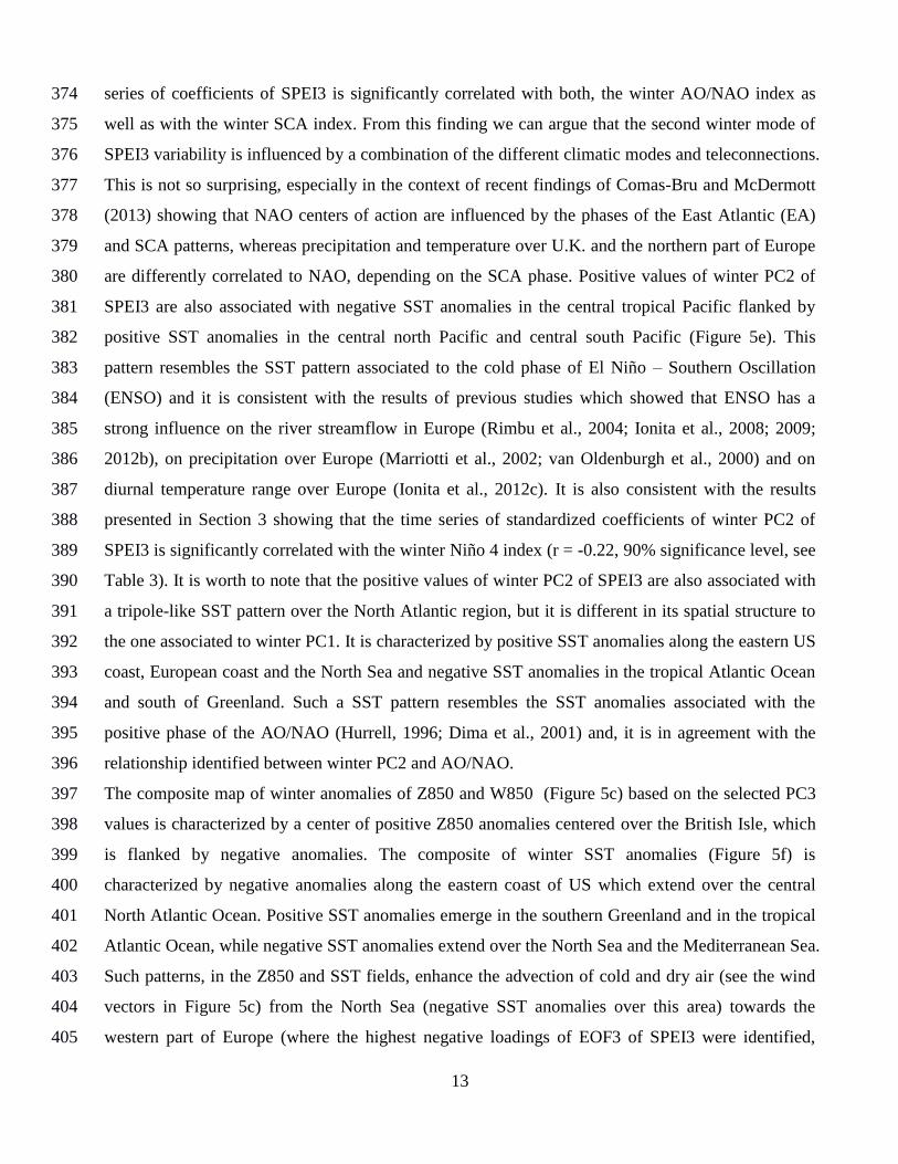
series of coefficients of SPEI3 is significantly correlated with both, the winter AO/NAO index as 374
well as with the winter SCA index. From this finding we can argue that the second winter mode of 375
SPEI3 variability is influenced by a combination of the different climatic modes and teleconnections. 376
This is not so surprising, especially in the context of recent findings of Comas-Bru and McDermott 377
(2013) showing that NAO centers of action are influenced by the phases of the East Atlantic (EA) 378
and SCA patterns, whereas precipitation and temperature over U.K. and the northern part of Europe 379
are differently correlated to NAO, depending on the SCA phase. Positive values of winter PC2 of 380
SPEI3 are also associated with negative SST anomalies in the central tropical Pacific flanked by 381
positive SST anomalies in the central north Pacific and central south Pacific (Figure 5e). This 382
pattern resembles the SST pattern associated to the cold phase of El Niño – Southern Oscillation 383
(ENSO) and it is consistent with the results of previous studies which showed that ENSO has a 384
strong influence on the river streamflow in Europe (Rimbu et al., 2004; Ionita et al., 2008; 2009; 385
2012b), on precipitation over Europe (Marriotti et al., 2002; van Oldenburgh et al., 2000) and on 386
diurnal temperature range over Europe (Ionita et al., 2012c). It is also consistent with the results 387
presented in Section 3 showing that the time series of standardized coefficients of winter PC2 of 388
SPEI3 is significantly correlated with the winter Niño 4 index (r = -0.22, 90% significance level, see 389
Table 3). It is worth to note that the positive values of winter PC2 of SPEI3 are also associated with 390
a tripole-like SST pattern over the North Atlantic region, but it is different in its spatial structure to 391
the one associated to winter PC1. It is characterized by positive SST anomalies along the eastern US 392
coast, European coast and the North Sea and negative SST anomalies in the tropical Atlantic Ocean 393
and south of Greenland. Such a SST pattern resembles the SST anomalies associated with the 394
positive phase of the AO/NAO (Hurrell, 1996; Dima et al., 2001) and, it is in agreement with the 395
relationship identified between winter PC2 and AO/NAO. 396
The composite map of winter anomalies of Z850 and W850 (Figure 5c) based on the selected PC3 397
values is characterized by a center of positive Z850 anomalies centered over the British Isle, which 398
is flanked by negative anomalies. The composite of winter SST anomalies (Figure 5f) is 399
characterized by negative anomalies along the eastern coast of US which extend over the central 400
North Atlantic Ocean. Positive SST anomalies emerge in the southern Greenland and in the tropical 401
Atlantic Ocean, while negative SST anomalies extend over the North Sea and the Mediterranean Sea. 402
Such patterns, in the Z850 and SST fields, enhance the advection of cold and dry air (see the wind 403
vectors in Figure 5c) from the North Sea (negative SST anomalies over this area) towards the 404
western part of Europe (where the highest negative loadings of EOF3 of SPEI3 were identified, 405
14
Figure 1c) favoring dry conditions over these regions. These results are in line with the findings of 406
Madden and Williams (1977) showing that during winter months, cold and dry air has the tendency 407
to suppress precipitation, especially over the European continent. 408
409
4.2 Spring 410
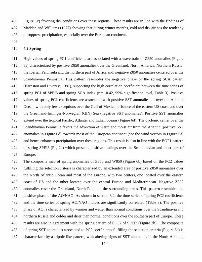
High values of spring PC1 coefficients are associated with a wave train of Z850 anomalies (Figure 411
6a) characterized by positive Z850 anomalies over the Greenland, North America, Northern Russia, 412
the Iberian Peninsula and the northern part of Africa and, negative Z850 anomalies centered over the 413
Scandinavian Peninsula. This pattern resembles the negative phase of the spring SCA pattern 414
(Barnston and Livezey, 1987), supporting the high correlation coefficient between the time series of 415
spring PC1 of SPEI3 and spring SCA index (r = -0.42, 99% significance level, Table 3). Positive 416
values of spring PC1 coefficients are associated with positive SST anomalies all over the Atlantic 417
Ocean, with only few exceptions over the Gulf of Mexico, offshore of the eastern US coast and over 418
the Greenland-Irminger-Norwegian (GIN) Sea (negative SST anomalies). Positive SST anomalies 419
extend over the tropical Pacific, Atlantic and Indian oceans (Figure 6d). The cyclonic center over the 420
Scandinavian Peninsula favors the advection of warm and moist air from the Atlantic (positive SST 421
anomalies in Figure 6d) towards most of the European continent (see the wind vectors in Figure 6a) 422
and hence enhances precipitation over these regions. This result is also in line with the EOF1 pattern 423
of spring SPEI3 (Fig 2a) which presents positive loadings over the Scandinavian and most part of 424
Europe. 425
The composite map of spring anomalies of Z850 and W850 (Figure 6b) based on the PC2 values 426
fulfilling the selection criteria is characterized by an extended area of positive Z850 anomalies over 427
the North Atlantic Ocean and most of the Europe, with two centers, one located over the eastern 428
coast of US and the other located over the central Europe and Mediterranean. Negative Z850 429
anomalies cover the Greenland, North Pole and the surrounding areas. This pattern resembles the 430
positive phase of the AO/NAO. As shown in section 3.2, the time series of spring PC2 coefficients 431
and the time series of spring AO/NAO indices are significantly correlated (Table 3). The positive 432
phase of AO is characterized by warmer and wetter than normal conditions over the Scandinavia and 433
northern Russia and colder and drier than normal conditions over the southern part of Europe. These 434
results are also in agreement with the spring pattern of EOF2 of SPEI3 (Figure 2b). The composite 435
of spring SST anomalies associated to PC2 coefficients fulfilling the selection criteria (Figure 6e) is 436
characterized by a tripole-like pattern, with altering signs of SST anomalies in the North Atlantic, 437

15
similar to those corresponding to the positive phase of AO (Dima et al., 2001). Both the composites 438
of Z850(W850) and SST anomalies associated with high values of spring PC2 coefficients are 439
similar to the composites of Z850 (W850) and SST anomalies associated to high values of winter 440
PC2, implying a certain persistence from winter to spring of the driving factors and the climate 441
anomalies that are associated to them. 442
The composite map of spring anomalies of Z850 and W850 (Figure 6c) based on the PC3 values 443
fulfilling the selection criteria (Figure 6c) shows a tripole-like structure between the central North 444
Atlantic Ocean (negative anomalies), the British Isle and Western Europe (positive anomalies) and 445
eastern and south-eastern Europe and western Russia (negative anomalies). This spatial pattern 446
projects onto the positive phase of the Atlantic Multidecadal Oscillation and, it is associated with 447
reduced precipitation over the central Europe (Sutton and Dong, 2012) which is in agreement with 448
the negative loading of the spring EOF3 of SPEI3 (Figure 2c) identified over this regions. Moreover, 449
the dominant feature of the composite map of spring SST anomalies based on PC3 selected values 450
(Figure 6f) is the quasi-monopolar positive anomalies in the North Atlantic Ocean. As indicated by 451
other studies (Latif et al., 2004; Knight et al. 2005) such a quasi-monopolar structure is associated 452
with the extreme phases of the Atlantic Multidecadal Oscillation (AMO). This result is also certified 453
by the correlation coefficient between the time series of spring PC3 coefficients and the time series 454
of spring AMO index (r = 0.37, 99% significance level, Table 3) suggesting that the AMO could 455
play an important role in driving moisture variability over Europe. Positive (negative) SST 456
anomalies over the North Atlantic are associated with positive (negative) phase of AMO which 457
induce to dry (wet) conditions over the western Europe and wet (dry) conditions over the eastern 458
Europe and western Russia as also confirmed by the spring EOF3 loadings of SPEI3 (Figure 2c). 459
460
4.3 Summer 461
The composite map of summer anomalies of Z850 and W850 (Figure 7a) based on the PC1 values 462
fulfilling the selection criteria presents a large area of negative anomalies centered over Scandinavia 463
and the British Isles which extends westward over the North Atlantic and the eastern US. Another 464
center of positive anomalies is located over Greenland and adjacent areas, while another area of 465
positive anomalies, centered over the Mediterranean extends eastward to Eurasia. The composite 466
map of summer SST anomalies associated to positive values of PC1 values fulfilling the selection 467
criteria shows negative SST anomalies over the North Sea and along the western coast of 468
Scandinavia and positive SST anomalies along the southern coast of Greenland, central and tropical 469
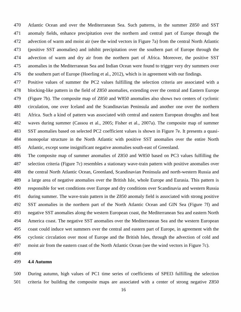
16
Atlantic Ocean and over the Mediterranean Sea. Such patterns, in the summer Z850 and SST 470
anomaly fields, enhance precipitation over the northern and central part of Europe through the 471
advection of warm and moist air (see the wind vectors in Figure 7a) from the central North Atlantic 472
(positive SST anomalies) and inhibit precipitation over the southern part of Europe through the 473
advection of warm and dry air from the northern part of Africa. Moreover, the positive SST 474
anomalies in the Mediterranean Sea and Indian Ocean were found to trigger very dry summers over 475
the southern part of Europe (Hoerling et al., 2012), which is in agreement with our findings. 476
Positive values of summer the PC2 values fulfilling the selection criteria are associated with a 477
blocking-like pattern in the field of Z850 anomalies, extending over the central and Eastern Europe 478
(Figure 7b). The composite map of Z850 and W850 anomalies also shows two centers of cyclonic 479
circulation, one over Iceland and the Scandinavian Peninsula and another one over the northern 480
Africa. Such a kind of pattern was associated with central and eastern European droughts and heat 481
waves during summer (Cassou et al., 2005; Fisher et al., 2007a). The composite map of summer 482
SST anomalies based on selected PC2 coefficient values is shown in Figure 7e. It presents a quasi-483
monopolar structure in the North Atlantic with positive SST anomalies over the entire North 484
Atlantic, except some insignificant negative anomalies south-east of Greenland. 485
The composite map of summer anomalies of Z850 and W850 based on PC3 values fulfilling the 486
selection criteria (Figure 7c) resembles a stationary wave-train pattern with positive anomalies over 487
the central North Atlantic Ocean, Greenland, Scandinavian Peninsula and north-western Russia and 488
a large area of negative anomalies over the British Isle, whole Europe and Eurasia. This pattern is 489
responsible for wet conditions over Europe and dry conditions over Scandinavia and western Russia 490
during summer. The wave-train pattern in the Z850 anomaly field is associated with strong positive 491
SST anomalies in the northern part of the North Atlantic Ocean and GIN Sea (Figure 7f) and 492
negative SST anomalies along the western European coast, the Mediterranean Sea and eastern North 493
America coast. The negative SST anomalies over the Mediterranean Sea and the western European 494
coast could induce wet summers over the central and eastern part of Europe, in agreement with the 495
cyclonic circulation over most of Europe and the British Isles, through the advection of cold and 496
moist air from the eastern coast of the North Atlantic Ocean (see the wind vectors in Figure 7c). 497
498
4.4 Autumn 499
During autumn, high values of PC1 time series of coefficients of SPEI3 fulfilling the selection 500
criteria for building the composite maps are associated with a center of strong negative Z850 501

17
anomalies located over the Scandinavian Peninsula and north-western Europe which extends up to 502
central and eastern Europe (Figure 8a). This area of Z850 negative anomalies is surrounded by a 503
large area of positive anomalies extended over the Greenland and Kara Sea, central North Atlantic 504
and northern Africa, Middle East and Eurasia (Figure 8a). This pattern results in a strong pressure 505
gradient between the centers of action, with the highest gradient over the north-western part of 506
Europe. Positive values of autumn PC1 coefficients fulfilling the selection criteria are also 507
associated with negative SST anomalies along the eastern US coast and the western European coast 508
which extend up to the north-western African coast and, an area of negative SST anomalies in the 509
center of North Pacific Ocean (Figure 8a). The composite map of the autumn SST anomalies 510
associated with selected coefficients of the PC1 fulfilling the criteria is characterized by positive 511
SST anomalies in the central North Atlantic extending northward up to the southern Greenland. 512
Outside these areas the SST anomalies are almost insignificant. A similar SST pattern was found to 513
influence the streamflow variability of Rhine River in autumn (Ionita et al., 2012b) and can be 514
obtained by applying an EOF analysis over the autumn SST anomalies over the North Atlantic 515
region and retaining the fourth leading EOF. The atmospheric circulation anomalies and the SST 516
anomalies identified and presented in Figures 8a and d, respectively, favor the advection of moist air, 517
and hence increased precipitation, towards the central part of Europe while the advection of dry air 518
from the northern part of Africa towards the southern part of Europe turns out in reduced 519
precipitation over these regions (see the wind vectors in Figure 8a). 520
The composite map of autumn Z850 anomalies based on the selected PC2 coefficients points out on 521
a large area of positive anomalies with two centers, one over the north-eastern US coast and the 522
other over the southern Europe. Negative Z850 anomalies associated with a cyclonic circulation are 523
centered northward of Scandinavia and extend over the northern part of the North Atlantic Ocean 524
and Greenland (Figure 8b). This pattern projects onto the positive phase of autumn NAO, which is 525
also in agreement with the significant correlation between the time series of autumn PC2 of SPEI3 526
and the time series of autumn NAO and AO indices (r = 0.37/0.52, 99% significant level, Table 3). 527
The composite map of the autumn SST anomalies based on selected PC2 coefficients (Figure 8e) is 528
characterized by negative SST anomalies around Iceland and tropical Atlantic and Pacific Oceans, 529
and positive SST anomalies over the central North Atlantic off shore the eastern US and western 530
European coasts, and the Mediterranean Sea. A warm Mediterranean Sea favors dry conditions over 531
the southern and south-eastern Europe while the cold North Sea is associated with wetter conditions 532
over the Scandinavian Peninsula and Great Britain. 533

18
The composite map of autumn Z850 and W850 anomalies associated to selected PC3 coefficients 534
fulfilling the selection criteria shows a wave train pattern characterized by a sequence of centers of 535
positive and negative Z850 anomalies: one center of negative anomalies over the central Atlantic 536
Ocean, one center of positive anomalies located over the British Isle and western Europe which is 537
connected with another center of positive anomalies located over the Mediterranean and northern 538
Africa and, a center of strong negative anomalies located over the north-western Russia (Figure 8c). 539
This pattern resembles the negative phase of the autumn SCA pattern, which was found to be 540
significantly correlated with the time series of autumn PC3 of SPEI3 (r = -0.39, Table 3). The 541
composite map of the autumn SST anomalies associated to the selected PC3 coefficients presents 542
positive SST anomalies along the eastern US and western European coast and negative SST 543
anomalies over the central North Atlantic Ocean and the Mediterranean Sea (Figure 8f). Such a 544
pattern of SST anomalies could drive/induce dry conditions over the central Europe and wet 545
conditions over the Eastern Europe during autumn. 546
5. Relationship with Rainday Counts, Cloud Cover and Soil Moisture 547
In this section the relationship between the seasonal SPEI3 variability and three fields of 548
climatological variables which are rainday counts (WET), cloud cover (CLD) and soil moisture 549
(SOIL) is analyzed in terms of correlation maps between the first three PCs for each season and 550
WET, CLD and SOIL fields. The results of the correlation analysis are shown in Figures 9 – 12, in 551
which the correlations that are exceeding the 95% significance level are hatched. 552
An increase in air temperature associated with reduced precipitation, which are the main factors 553
driving the drought conditions, can be the result of reductions of cloudiness, especially during spring 554
and summer (Tang et al., 2010). The increase in temperature (which is an important input variable in 555
the computation of SPEI) could also be enhanced by soil moisture reduction, which in turn reduces 556
the evaporation and evaporative cooling on the surface. However, during the winter months positive 557
temperature anomalies are associated with enhanced precipitation, due to the fact that the water 558
holding capacity of the atmosphere limits precipitation amounts during cold conditions (Trenberth 559
and Shea, 2005). 560
Soil moisture information has the potential to play an important role in predicting the occurrence of 561
drought phenomena and to improve the seasonal prediction of precipitation (Dirmeyer and Brubaker, 562
1999; Reichle and Koster, 2003). The influence of soil moisture has been studied especially 563
regarding the pre-conditioning in the context of heat waves and summer droughts (Zampieri et al., 564
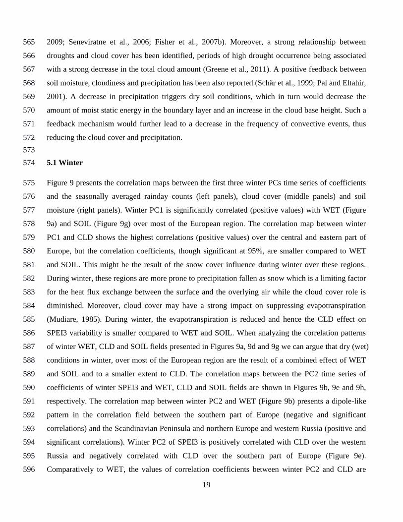
19
2009; Seneviratne et al., 2006; Fisher et al., 2007b). Moreover, a strong relationship between 565
droughts and cloud cover has been identified, periods of high drought occurrence being associated 566
with a strong decrease in the total cloud amount (Greene et al., 2011). A positive feedback between 567
soil moisture, cloudiness and precipitation has been also reported (Schär et al., 1999; Pal and Eltahir, 568
2001). A decrease in precipitation triggers dry soil conditions, which in turn would decrease the 569
amount of moist static energy in the boundary layer and an increase in the cloud base height. Such a 570
feedback mechanism would further lead to a decrease in the frequency of convective events, thus 571
reducing the cloud cover and precipitation. 572
573
5.1 Winter 574
Figure 9 presents the correlation maps between the first three winter PCs time series of coefficients 575
and the seasonally averaged rainday counts (left panels), cloud cover (middle panels) and soil 576
moisture (right panels). Winter PC1 is significantly correlated (positive values) with WET (Figure 577
9a) and SOIL (Figure 9g) over most of the European region. The correlation map between winter 578
PC1 and CLD shows the highest correlations (positive values) over the central and eastern part of 579
Europe, but the correlation coefficients, though significant at 95%, are smaller compared to WET 580
and SOIL. This might be the result of the snow cover influence during winter over these regions. 581
During winter, these regions are more prone to precipitation fallen as snow which is a limiting factor 582
for the heat flux exchange between the surface and the overlying air while the cloud cover role is 583
diminished. Moreover, cloud cover may have a strong impact on suppressing evapotranspiration 584
(Mudiare, 1985). During winter, the evapotranspiration is reduced and hence the CLD effect on 585
SPEI3 variability is smaller compared to WET and SOIL. When analyzing the correlation patterns 586
of winter WET, CLD and SOIL fields presented in Figures 9a, 9d and 9g we can argue that dry (wet) 587
conditions in winter, over most of the European region are the result of a combined effect of WET 588
and SOIL and to a smaller extent to CLD. The correlation maps between the PC2 time series of 589
coefficients of winter SPEI3 and WET, CLD and SOIL fields are shown in Figures 9b, 9e and 9h, 590
respectively. The correlation map between winter PC2 and WET (Figure 9b) presents a dipole-like 591
pattern in the correlation field between the southern part of Europe (negative and significant 592
correlations) and the Scandinavian Peninsula and northern Europe and western Russia (positive and 593
significant correlations). Winter PC2 of SPEI3 is positively correlated with CLD over the western 594
Russia and negatively correlated with CLD over the southern part of Europe (Figure 9e). 595
Comparatively to WET, the values of correlation coefficients between winter PC2 and CLD are 596

20
much smaller. The pattern of the correlation map between winter PC2 and SOIL (Figure 9h) is much 597
alike with the WET correlation map (Figure 9b) and with the pattern of winter EOF2 (Figure 1b). As 598
in the case of PC1, WET and SOIL show a higher influence on moisture conditions compared to 599
CLD and, we speculate that this result can be attributed to the direct effect of snow cover. Moisture 600
conditions over the southern part of Europe are sensitive to WET, CLD and SOIL, while over the 601
Scandinavian Peninsula they are more sensitive to WET and SOIL and less sensitive to CLD. In the 602
case of PC3 time series of coefficients, the correlation maps with WET (Figure 9c) and SOIL 603
(Figure 9i) show a similar pattern of correlation characterized by negative correlations over the 604
Iberian Peninsula, British Isle and southern Scandinavian Peninsula and positive correlations over 605
the eastern Europe and Russia which is in agreement with the pattern of winter EOF3 of SPEI3 606
(Figure 1c). The correlation map between winter PC3 time series of coefficients and CLD (Figure 9f) 607
is different compared to WET and SOIL and shows strong and significant negative correlation over 608
the northern Europe, western Russia and the southern part of the Scandinavian Peninsula. This 609
difference can be due to complex large-scale and regional factors that influence moisture conditions. 610
One of the reason for which the correlation with CLD is smaller in winter can be due to the fact that 611
SPEI3 is based on potential evapotranspiration (PET) and, it was reported that PET is sensitive to 612
CLD mainly in spring and summer (Tang et al., 2010, Ionita et al., 2012c). 613
5.2 Spring 614
During spring, the PC1 time series of coefficients is significantly correlated with the WET field 615
(significant and positive correlations up to ~ 0.7) over large areas including the central and northern 616
part of Europe, western Russia and the Scandinavian Peninsula (Figure 10a) and negatively 617
correlated over the Iberian Peninsula, southernmost part of Europe and the Middle East. The 618
correlation map between spring PC1 and spring CLD (Figure 10d) is similar to the correlation map 619
of WET (Figure 10a) but the correlation coefficients are smaller compared to WET, though still 620
significant. Dry (wet) conditions over the central and western part of Europe and western Russia are 621
associated with decreased (increased) soil moisture content over these regions. The correlation map 622
for SOIL also shows a low negative correlation along the western and northern coast of the 623
Scandinavian Peninsula. This aspect may be due to the fact that the western coast of Scandinavian 624
Peninsula is a mountain region and most of the soils are formed on glacial materials (Jones et al., 625
2005) and the bedrock is calcareous, this characteristic making these soils less sensitive to moisture. 626
The correlation maps between the spring PC2 series of coefficients and spring WET (Figure 10b), 627
21
spring CLD (Figure 10e) and spring SOIL (Figure 10h) present similar correlation patterns. Dry 628
(wet) conditions over the southern and central part of Europe (the Scandinavian Peninsula) are 629
associated with reduced (enhanced) rainday counts (Figure 10b), low (high) cloudiness (Figure 10e) 630
and decreased (increased) soil moisture content (Figure 10h). In the case of spring PC2 all three 631
considered parameters (WET, CLD and SOIL) seem to play an important role on determining 632
dryness/wetness conditions over the analyzed regions, in terms of correlation coefficients. Figures 633
10c, 10f and 10i present the correlation maps between the spring PC3 time series of coefficients and 634
WET field (Figure 10c), CLD field (Figure 10f) and SOIL field (Figure 10i). The regions exhibiting 635
the highest correlations between spring PC3 and WET (Figure 10c), CLD (Figure 10f) and SOIL 636
(Figure 10i) are the Eastern Europe and western Russia (positive correlations) and Western Europe 637
(negative correlations). Dry (wet) conditions over the western Russia and Eastern Europe are 638
associated with decreased (increased) rainday counts, low (high) cloudiness and reduced (enhanced) 639
soil moisture content over these regions. As in the case of the winter season, the correlation between 640
the spring PCs and spring CLD were smaller compared to spring WET and spring SOIL, especially 641
over the northern part of Europe (areas which in spring can still be covered by snow, Brown and 642
Robinson, 2011). Again, we can speculate that these results can be an effect of the influence of snow 643
cover, which acts as a barrier between the surface layer and the overlying air. 644
5.3 Summer 645
Figures 11a, 11d and 11g present the correlation maps between the summer PC1 time series of 646
coefficients and the summer WET, CLD and SOIL fields. The correlation patterns show a dipole-647
like structure, with the highest positive correlations over the northern part of Europe, western Russia 648
and the Scandinavian Peninsula and negative correlations over the southern part of Europe. The 649
magnitudes of the correlation coefficients are almost the same for all three analyzed fields (WET, 650
CLD and SOIL). Wet (dry) conditions over the northern part of Europe, Scandinavian Peninsula and 651
western part of Russia are associated with enhanced (reduced) rainday counts (Figure 11a), high 652
(low) cloudiness (Figure 11d) and increased (decreased) soil moisture content (Figure 11g) over 653
these regions. For the southern part of Europe dry (wet) conditions are associated with reduced 654
(enhanced) rainday counts, low (high) cloudiness and decreased (increased) soil moisture content. 655
The correlation map of summer PC2 with WET (Figure 11b) and CLD (Figure 11e) fields shows the 656
highest negative (positive) correlations over western Russia (Scandinavian Peninsula, Western 657
Europe and Turkey), while in the case of SOIL field, the correlation map shows significant negative 658

22
correlations over western Russia and positive correlations only over small regions (Turkey and 659
northern part of Sweden). This is not surprisingly, since the highest negative loadings of summer 660
EOF2 are found over western Russia. Therefore, enhanced (reduced) rainday counts, high (low) 661
cloudiness and increased (decreased) soil moisture anomalies lead to wet (dry) periods over most of 662
the western part of Russia. The correlation coefficients between summer PC3 series of coefficients 663
with WET, CLD and SOIL fields are positive and significant over most of continental part of 664
Europe and southern Scandinavian Peninsula. Over the north-western part of Russia the correlation 665
is negative. In terms of correlation coefficients values the influence of CLD and SOIL on moisture 666
conditions over the north-western part of Russia is much smaller compared to WET. Tang et al. 667
(2012) showed that over this region the summer temperature (which is an integrated part in the 668
definition of SPEI) is more sensitive to precipitation variability than to cloud cover and, this could 669
also explain the highest correlation between summer PC3 and WET over north-western Russia. 670
5.4 Autumn 671
Figures 12a, 12d and 12g show the correlation maps between the autumn PC1 time series of 672
coefficients and the autumn WET, CLD and SOIL fields, respectively. The correlation maps show a 673
pattern of positive (negative) correlation with the highest positive significant values centered over 674
the northern part of Europe, the Scandinavian Peninsula and western part of Russia (southern part of 675
Europe). The highest correlations are found between the autumn PC1 time series and WET and 676
SOIL (Figures 12a and 12g, respectively). The autumn PC2 time series of coefficients is negatively 677
correlated with WET (Figure 12b), CLD (Figure 12f) and SOIL (Figure 12h) over most of the part 678
of Europe and positively correlated with WET and SOIL over the Scandinavian Peninsula and 679
northern Russia. The correlation maps between the PC3 time series of coefficients and seasonally 680
averaged WET, CLD and SOIL are presented in Figures 12c, 12f and 12i, respectively. They are 681
very similar in the spatial distribution of correlation coefficients though the highest correlation 682
coefficients are recorded between the autumn PC3 and WET (Figure 12c). Dry (wet) conditions over 683
the western part of Europe are associated with reduced (enhanced) rainday counts, low (high) 684
cloudiness and decreased (increased) soil moisture anomalies. At the same time, wet (dry) 685
conditions over the western part of Russia are associated with enhanced (reduced) rainday counts, 686
high (low) cloudiness and increased (decreased) soil moisture content. As in the case of summer, the 687
correlation coefficients between the autumn PC3 time series of SPEI3 and WET and SOIL is 688
stronger compared to CLD. 689
23
6. Discussion 690
As a complex natural hazard, drought is best characterized by multiple climatological and 691
hydrological parameters, therefore is very important to understand the association of drought with 692
climatic, oceanic and local factors. Persistent dry (wet) conditions are usually associated with 693
persistent anticyclones (cyclones) (Schubert et al., 2014), while the sea surface temperature plays 694
also an important role on dryness and wetness variability, via large scale climate modes of 695
variability (e.g. AMO and/or ENSO) (Ionita et al., 2012a). 696
In this study the spatio-temporal variability of the seasonal short-term dryness and wetness 697
conditions as represented by SPEI3 over the European region are investigated, and the relationship 698
with large-scale factors is highlighted. There are relatively few studies that assess this relationship 699
and most of them are either restricted to areas prone to drought (Iberian Peninsula, Mediterranean 700
region or the southern part of Europe) or to a particular season (mostly summer). A strong 701
relationship between the seasonal variability of temperature and precipitation, which are key factors 702
in driving the dryness and wetness conditions, and the global atmospheric circulation, has already 703
been reported (Hurrell et al., 1995; Slonosky et al., 2001; Zveryaev et al., 2006, 2009; Sutton and 704
Hodson, 2005). The aim of this study is to provide more insights on the seasonal dryness/wetness 705
variability over the European region based on the analysis of SPEI3 which is an index that quantifies 706
the moisture status based on temperature and precipitation. 707
During the winter season the variability of SPEI3 was found to be linked to well-known climate 708
modes: AO/NAO, SCA, EAWR and EA. Moreover, in our study we showed that the combined 709
effect of these climate modes (NAO vs. SCA and EAWR), not just NAO, may have quite a strong 710
impact on SPEI3 variability. This is a very important result, especially in the view of the recent 711
findings of Comas-Bru and McDermott (2013), who showed that the NAO centers of actions are 712
influence by the phase of the SCA and the EA patterns. Although NAO is one of the most 713
prominent teleconnection patterns in all seasons (Barnston and Livezey, 1987), its relative role in 714
regulating the variability of the European climate during non-winter months is not that clear as for 715
the winter season. At the same time, the mechanisms which drive the European climate variability 716
might vary from one climatic period to another and, also, they might be different for different 717
variables (e.g. precipitation, streamflow, air temperature and drought). 718
The winters PCs series of coefficients are associated with cyclonic (anticyclonic) circulations over 719
the regions where the corresponding EOFs have the highest positive (negative) loadings. According 720
to the composite maps of Z850, W850 and SST anomalies based on the selected values of winter 721
24
PC1, the cyclonic circulation is associated with the advection of warm air from the Atlantic Ocean 722
(positive SST anomalies) and with higher rainday counts and higher cloudiness, which in turn are 723
responsible for the wet periods over these regions. The winter PC1 of SPEI3 was found to be more 724
correlated with winter WET and SOIL than with CLD. Reduced (enhanced) rainday counts together 725
with decreased (increased) soil moisture content contribute to a higher degree to drought variability 726
during winter compared to low (high) cloud cover. The influence of the cloud cover can be 727
diminished by the presence of snow cover, which can limit the heat flux exchange between the 728
surface and the overlying air. 729
As in the case of winter season, dryness and wetness variability during spring is strongly related to 730
climatic modes of variability. The leading mode of spring variability of SPEI3 is positively 731
correlated with the EA mode and negatively correlated with POL and SCA modes. According to the 732
second mode of spring variability of SPEI3, dry (wet) conditions over the central and southern part 733
of Europe (Scandinavian Peninsula) are associated with an atmospheric circulation mode that 734
projects onto the positive phase of AO/NAO modes. Also, the spring PC2 time series of coefficients 735
is negatively correlated with the SCA mode. The spring PC3 time series of coefficients of SPEI3 is 736
positively correlated with AMO and negatively correlated with NAO and SCA. AMO was found to 737
play an important role in the modulation of the European climate, especially during summer (Sutton 738
and Hodson, 2005; Ionita et al., 2013). Recent studies showed that AMO can modulate the climate 739
variability over Europe also during the transition seasons (Ionita et al., 2012c; Sutton and Dong, 740
2012). In general, high values of SPEI3 were associated with positive anomalies of rainday counts; 741
cloud cover and soil moisture content over the regions were the highest positive loadings are found 742
in the EOF maps. The highest correlation of spring PCs time series of coefficients was identified 743
with the WET field compared with CLD and SOIL. Nevertheless, CLD and SOIL plays also a 744
significant role in spring dryness and wetness variability, but the correlations, though significant, are 745
smaller compared to WET field. 746
The pattern of the first mode of SPEI3 variability over Europe during summer is also the result of 747
the influence of various teleconnection patterns. The summer PC1 of SPEI3 is negatively correlated 748
with the NAO/AO, EAWR and SCA, and positively correlated with the EA. The influence of these 749
large scale teleconnection modes resulted in a spatial distribution of the Z850 anomalies in a wave 750
train pattern characterized by a center of positive anomalies over Greenland, a center of negative 751
anomalies over the central North Atlantic extending up to the Scandinavian Peninsula and another 752
center of positive anomalies over the Mediterranean Sea extending up to central Russia. Such kind 753

25
of circulation pattern favors the advection of warm and dry air from the northern part of Africa 754
towards the southern part of Europe (see the wind vectors in the composite maps), which in turn will 755
experience dry conditions. It is well known that the atmospheric circulation during summer seasons 756
is mostly influenced by the atmospheric blocking as it was shown in the composite map of Z850 757
anomalies associated to PC2 series of coefficients. Most of the extreme events related to heat waves 758
in Europe, during summer, were triggered by such a particular atmospheric pattern. Anomalously 759
barotropic structures are particularly strong (weak) in June (July) when the large scale anomalies are 760
organized in wave trains that propagate from the Atlantic Ocean towards the European continent 761
(Xopalki et al., 1995; Corte-Real et al., 1995; Cassou et al., 2005). Summer dry conditions over 762
western Russia are associated with a blocking like pattern over Europe It is characterized by an 763
anticyclonic circulation over the eastern part of Europe and two centers of cyclonic circulation, one 764
over the Scandinavian Peninsula and the British Isles, and another one over the northern part of 765
Africa. Such a pattern of atmospheric blocking was responsible for one of the most extreme 766
summer heat waves recorded over the eastern Europe and Russia during 2010 (Dole et al., 2011). In 767
general, the atmospheric blocking in summer is associated with extreme temperatures and heat 768
waves (Della-Marta et al., 2007, Garcia-Herrera et al., 2010; Feudale and Shukla, 2010). During 769
summer, the correlation maps of PCs time series of coefficients with WET, CLD and SOIL show 770
similar patterns (in terms of amplitude of the correlation coefficients) but the strength and the 771
significance of the correlation coefficients demonstrate that the WET and SOIL fields have more 772
influence on moisture variability than CLD. 773
The first mode of autumn moisture variability was found to be significantly correlated with the 774
autumn POL and EAWR teleconnection patterns. The second mode of autumn moisture variability 775
is strongly related to AO/NAO modes, as in the case of winter EOF2. Dry (wet) conditions over 776
central and the southern part of Europe (Scandinavian Peninsula) are associated with Z850 and SST 777
anomalies that project onto the positive phase of AO/NAO. The third mode of the autumn variability 778
of SPEI3 is the result of the influence of various teleconnection patterns. The PC3 is positively 779
correlated with NAO/AO and negatively correlated with SCA. The composite of Z850 anomalies 780
based on selected PC3 values presents a wave train pattern (with altering signs) which develops over 781
the Atlantic Ocean and extends up to Siberia. Higher correlations have been identified between the 782
autumn PCs and WET and SOIL fields compared to CLD. 783
784

26
7. Conclusions 785
The mains conclusions of our study can be summarized as follows: 786
The leading modes of SPEI3 variability are definitely seasonally – dependent. Although the 787
spatial structure of the leading modes of seasonal variability of SPEI3 may show 788
resemblance between each other, the temporal evolution (in terms of principal component 789
time series of coefficients) differs significantly from one season to another. Moreover, the 790
leading modes of dryness and wetness variability quantified by SPEI3 are associated with 791
particular atmospheric circulation patterns and sea surface temperature anomalies for each 792
season. The analysis of seasonal composite maps of Z850, W850 and global SST anomalies 793
and of seasonal correlation maps of the first three PCs of SPEI3 and WET, CLD and SOIL 794
fields pointed out on a specific and significant role of each of these climatic variables on the 795
seasonal short-term SPEI3 variability. 796
The response of dryness/wetness variability quantified by SPEI3 to SST anomalies was 797
found to be more regional during summer, compared to other seasons. This might be due to 798
the fact that during summer moisture conditions are more sensitive to local conditions (e.g. 799
precipitation, soil moisture). Another reason might be that the response of air temperature 800
over the land (which is an input parameter for the computation of SPEI) to SST anomaly 801
variations is seasonally dependent and, this seasonality is mainly due to the warming trends 802
of SST (Cattiaux et al., 2010). 803
Overall, the correlation maps between the PC time series of coefficients corresponding to the 804
three leading modes of seasonal SPEI3 variability and the fields of WET, CLD and SOIL 805
show much similarities with the patterns of EOF loadings, meaning that the regions with the 806
highest loadings in the EOF field are similar to the regions where the highest correlation is 807
recorded in the correlation maps of the seasonal PCs with WET, CLD and SOIL fields. The 808
main difference arises from the fact that in some seasons and for particular regions WET and 809
SOIL show stronger influence (in terms of correlation coefficient amplitude) on 810
dryness/wetness conditions over Europe compared to CLD. This might be one of the direct 811
results of the fact that the SPEI3 variability is modulated both by local and large scale-812
factors. The differences in the correlation maps between seasonal PCs and WET, CLD and 813
SOIL fields might also be due to the different soil types that characterize different regions. 814
One specific example is the western part of the Scandinavian Peninsula, where the effect of 815
soil moisture is less that important due to the fact that the soils over these regions mainly 816
27
consist of glacial materials (which are not sensitive to soil moisture, Jones et al., 2005). 817
The findings of this paper also suggest that dryness and wetness variability over Europe is 818
influenced by rainday counts, cloud cover and soil moisture as a direct result of atmospheric 819
circulation anomalies. The physical mechanisms involved in dryness/wetness variability are 820
very complex and differ from one season to another. Precipitation deficits can be induced by 821
various processes including decreasing cloudiness, and land surface drying can slack 822
evapotranspiration and thus inhibiting cloud formation. This can be the result of the direct 823
effect of atmospheric factors (e.g. cyclones and anticyclones) and global and/or regional SST 824
anomalies. Moreover, when studying the variability of the moisture in connection to large 825
scale circulation, one should take into account the soil characteristics to specific regions. 826
The main findings of this study are that the leading EOF modes of SPEI3 variability are 827
characterized by seasonal differences and, their relationship with the large-scale atmospheric 828
circulation, global SST, rainday counts, cloud cover and soil moisture is also seasonal - dependent. 829
The results presented here also point out on how complex the drivers of the dryness and wetness 830
variability at the European scale are. Given the complex nature of seasonal dryness/wetness 831
variability and the temporal scales of its potential impact on various socio-economic sectors, a next 832
logical step will be to perform a similar analysis for mid-range and long-term dryness and wetness 833
variability quantified with SPEI. 834
835
836
837
838
839
840
841
842
843
844
845
846
847
848

28
Acknowledgements. The work was supported by the REKLIM (Regionale Klimaänderungen/ 849
Regional climate change) project and Polar Regions and Coasts in a changing Earth System Project 850
(PACES II). 851
852
853
854
855
856
857
858
859
860
861
862
863
864
865
866
867
868
869
870
871
872
873
874
875
876
877
878
879
880
29
References 881
882
Alley WM (1984) The Palmer drought severity index: Limitations and applications. J Appl Meteor 883
23:1100–1109 884
Barnston AG, Livezey RE (1987) Classification, seasonality, and persistence of low-frequency 885
atmospheric circulation patterns. Mon Wea Rev 115:1083–1126 886
Boroneant, C, Potop V, Mozný M, Štepánek P, Skalák P (2012) Large scale circulation patterns 887
associated to seasonal dry and wet conditions over the Czech Republic. pp. 271-280 in 888
Cambio climático. Extremos e impactos. Publicaciones de la Asociación Española de 889
Climatología (AEC), 2012, Serie A, n. 8, Salamanca, 998 pp. ISBN: 978-84-695-4331-3. 890
Briffa KR, G. van der Schrier G, Jones PD (2009) Wet and dry summers in Europe since 1750: 891
evidence of increasing drought. Int J Climatology 29: 1894-190. 892
Brown, R. D. and Robinson, D. A.: Northern Hemisphere spring snow cover variability and change 893
over 1922–2010 including an assessment of uncertainty, The Cryosphere, 5, 219-229, 894
doi:10.5194/tc-5-219-2011, 2011. 895
Cai W, Cowan T (2008) Evidence of impacts from rising temperature on inflows to the Murray-896
Darling Basin. Geophys Res Lett 35: L07701 doi:10.1029/2008GL033390 897
Cassou C, Terray L, Phillips A (2005) Tropical Atlantic influence on European heat waves. J 898
Climate 18: 2011–2805 899
Cattiaux J., Vautard R, Yiou P (2010) North-Atlantic SST amplified recent wintertime European 900
land temperature extremes and trends. Clim Dyn 36(11–12): 2113–2128 doi: 901
10.1007/s00382-010-0869-0 902
Comas-Bru L, McDermott F (2013) Impacts of the EA and SCA patterns on the European twentieth 903
century NAO–winter climate relationship. QJR Meteorol Soc in press doi: 10.1002/qj.2158 904
Compo GP, Whitaker JS, Sardeshmukh PD (2006) Feasibility of a 100 year reanalysis using only 905
surface pressure data. Bull Amer Met Soc 87:175-190 906
Compo GP, Whitaker JS, Sardeshmukh PD, Matsui N, Allan RJ, Yin X, Gleason BE, Vose RS, 907
Rutledge G, Bessemoulin P, Brönnimann S, Brunet M, Crouthamel RI, Grant AN, Groisman 908
PY, Jones PD, Kruk M, Kruger AC, Marshall GJ, Maugeri M, Mok HY, NordlI Ø, Ross TF, 909
30
Trigo RM, Wang XL, Woodruff SD, Worley SJ(2011) The Twentieth Century Reanalysis 910
Project. QJR Meteorol Soc 137: 1-28. DOI: 10.1002/qj.776. 911
Corte-Real J, Zhang X, Wang X(1995) Large-scale circulation regimes and surface climatic 912
anomalies over the Mediterranean. Int J Climatol 15: 1135–1150 913
Dai A (2011a) Drought under global warming: a review. Wiley Interdiscip Rev Clim Chang 2:45–65 914
Dai A (2011b) Characteristics and trends in various forms of the Palmer Drought Severity Index 915
during 1900–2008. J Geophys Re, 116: D12115 doi:10.1029/2010JD015541 916
Della-Marta PM, Haylock MR, Luterbacher J, Wanner H (2007) Doubled length of western 917
European summer heat waves since 1880. J Geophys Res 112:D15103 918
Dima M, Rimbu N, Stefan S, Dima I (2001) Quasi-Decadal Variability in the Atlantic Basin 919
Involving Tropics–Midlatitudes and Ocean–Atmosphere Interactions. J Climate 14: 823–832. 920
Dirmeyer PA, Brubaker KL (1999) Contrasting evaporative moisture sources during the drought of 921
1988 and the flood of 1993. J Geophys Res 104(D16): 19383–19397 922
doi:10.1029/1999JD900222 923
Dole R, Hoerling M, Perlwitz J, Eischeid J, Pegion P, Zhang T, Quan XW, Xu T, Murray D (2011) 924
Was there a basis for anticipating the 2010 Russian heat wave? Geophys Res Lett 38: 925
L06702 doi:10.1029/2010GL046582 926
Enfield DB, Mestas-Nuñez AM, Trimble PJ (2001) The Atlantic Multidecadal Oscillation and its 927
relation to rainfall and river flows in the continental US. Geophys Res Lett 28: 2077–2080 928
Estrela MJ, Penarrocha D, Millan M (2000) Multi-annual drought episodes in the Mediterranean 929
(Valencia region) from 1950–1996. A spatio-temporal analysis. Int J Climatol 20:1599–1618 930
Farago T, Kozma E, Nemes C (1989) Drought indices in meteorology. Idojaras 93(1): 45–59 931
Feudale L, Shukla J (2010) Influence of sea surface temperature on the European heat wave of 2003 932
summer. Part I: An observational study. Clim Dyn 36: 1691–703 933
Fischer EM, Seneviratne SI, Vidale PL, Lüthi D, Schär C (2007a) Soil moisture–atmosphere 934
interactions during the 2003 European summer heat wave. J Climate 20: 5081–99 935
Fischer EM, Seneviratne SI, Lüthi D, Schär C (2007b) Contribution of land atmosphere coupling to 936
recent European summer heat waves. Geophys Res Lett 34: L06707 937
doi:10.1029/2006GL029068. 938
Folland CK, Karl TR, Christy JR, Clarke RA, Gruza GV, Jouzel J, Mann ME, Oerlemans J, 939
Salinger JM, Wang SW (2001) Observed climate variability and change. In Climate change 940
2001: The scientific basis. Contribution of Working Group I to the Third Assessment Report 941

31
of the Intergovernmental Panel on Climate Change, ed. J. T. Houghton, Y. Ding, D. J. 942
Griggs,M. Noguer, P. J. van der Linden, X. Dai, K.Maskell, and C.A. Johnson, 881. 943
Cambridge: Cambridge University Press. 944
Garcia-Herrera R, Diaz J, Trigo RM, Luterbacher J, Fischer EM (2010) A review of the European 945
summer heat wave of 2003. Critical Reviews in Environmental Science and Technology 40: 946
267-306 947
Greene H, Leighton HG, Stewart RE (2011) Drought and Associated Cloud Fields over the 948
Canadian Prairie Provinces. Atmosphere-Ocean 49 (4): 356-365 949
Harris I, Jones PD, Osborn TJ, Lister DH (2013) Updated high-resolution grids of monthly climatic 950
observations. In press Int J Climatol Doi: 10.1002/joc.3711 951
Heim RR (2002) A review of twentieth-century drought indices used in the United States. Bull Am 952
Meteorol Soc 83(8):1149–1165 953
Hurrel JW (1995) Decadal Trends in the North Atlantic Oscillation Regional Temperatures and 954
Precipitation. Science 269: 676–679 955
Hurrell JW (1996) Influence of variations in extratropical wintertime teleconnections on Northern 956
Hemisphere temperature. Geophys Res Lett 23: 665–668 957
Ionita M, Lohmann G, Rimbu N (2008) Prediction of Elbe discharge based on stable teleconnections 958
with winter global temperature and precipitation. J Climate 21: 6215-6226. 959
DOI:10.1175/2008JCLI2248.1 960
Ionita M, Rimbu N, Lohmann G (2011) Decadal variability of the Elbe River streamflow. Int J 961
Climatol 31 22–30 doi: 10.1002/joc.2054 962
Ionita M, Lohmann G, Rimbu N, Chelcea S, Dima M (2012a) Interannual to decadal summer 963
drought variability over Europe and its relationship to global sea surface temperature. Clim 964
Dyn 38(1–2):363–377 965
Ionita M, Lohmann G, Rimbu N, Chelcea S (2012b) Interannual Variability of Rhine River 966
Streamflow and Its Relationship with Large-Scale Anomaly Patterns in Spring and Autumn. 967
J Hydrometeor 13: 172–188 968
Ionita M, Lohmann G, Rimbu N, Scholz P (2012c) Dominant modes of Diurnal Temperature Range 969
variability over Europe and their relationships with large-scale atmospheric circulation and 970
sea surface temperature anomaly patterns. J Geophys Res doi:10.1029/2011JD016669 in 971
press 972
32
Ionita M, Rimbu N, Chelcea S, Patrut S (2013) Multidecadal variability of summer temperature over 973
Romania and its relation with Atlantic Multidecadal Oscillation. Theor and Appl Clim 974
113:305–315 975
Jones, R.J.A., Houšková, B., Bullock P. and Montanarella L. (eds) 2005. Soil Resources of Europe, 976
second edition. European Soil Bureau Research Report No.9, EUR 20559 EN, 420pp. Office 977
for Official Publications of the European Communities, Luxembourg 978
Jones PD, Moberg A (2003) Hemispheric and Large-Scale Surface Air Temperature Variations: An 979
Extensive Revision and an Update to 2001. J Climate 16: 206–223 980
Knight JR, Allan RJ, Folland CK, Vellinga M, Mann ME (2005) A signature of persistent natural 981
thermohaline circulation cycles in observed climate. Geophys Res Lett 32 L20708 982
doi:10.1029/2005GL024233 983
Koleva E, Alexandrov V (2008) Drought in the Bulgarian low regions during the 20th century. 984
Theor Appl Climatol 92:113–120 985
Latif M, Roeckner E, Botzet M, Esch M, Haak H, Hagemann S, Jungclaus J, Legutke S, Marsland S, 986
Mikolajewicz U, Mitchell JFB (2004) Reconstructing, monitoring, and predicting 987
multidecadal-scale changes in the North Atlantic thermohaline circulation with sea surface 988
temperature. J Climate 17: 1605–1614 989
Livada I, Assimakopoulos VD (2007) Spatial and temporal analysis of drought in Greece using the 990
Standardized Precipitation Index (SPI). Theor Appl Climatol 89:143–153 991
Lloyd-Hughes B, Saunders MA (2002) A drought climatology for Europe. Int J Climatol 22:1571–992
1592 993
Madden R.A., J. Williams, 1978: The Correlation between Temperature and Precipitation in the 994
United States and Europe. Mon. Wea. Rev., 106, 142–147. 995
Maracchi G (2000) Agricultural drought – a practical approach to definition, assessment and 996
mitigation strategies. In: Vogt JV, Somma F (eds) Drought and drought mitigation in Europe. 997
Advances in Natural and Technological Hazards Research, vol. 14. Kluwer Acad Publ: 63–998
75 999
Mariotti A, Zeng N, Lau K-M, (2002) Euro-Mediterranean rainfall and ENSO - a seasonally varying 1000
relationship. Geophys Res Lett 29 (12) 10.1029/2001GL014248 1001
McKee TBN, Doesken J, Kleist J (1993) The relationship of drought frequency and duration to time 1002

33
scales. Proc Eight Conf on Applied Climatology. Anaheim, CA, Amer. Meteor. Soc. 179–1003
184 1004
Mesta-Nuñez AM, Enfield DB (1999) Rotated global modes of non-ENSO sea surface temperature 1005
variability. J Climate 12: 2734-2746 1006
Mudiare O (1985) Influence of Light Rainfall Activity and Cloud Cover on Evapotranspiration 1007
Demands. Ph.D. Thesis, University of Saskatchewan, Saskatoon, SK. p. 105. 1008
Nicholls N (2004) The changing nature of Australian droughts. Clim Change 63: 323−326 1009
Pal JS, Eltahir EAB (2001) Pathways relating soil moisture conditions to future summer rainfall 1010
within a model of the land-atmosphere system. J Climate 14: 1227–1242 1011
Palme WC (1965) Meteorological Drought. Res Paper No. 45 Weather Bureau Washington D.C. 58 1012
pp. 1013
Ped DA (1975) On parameters of drought and humidity. Papers of the USSSR hydrometeorological 1014
center 156: 19–38 (in Russian) 1015
Potop V., Boroneanţ C., Mozný M., Štepánek P., Skalák P. (2013) Observed spatiotemporal 1016
characteristics of drought on various time scales over the Czech Republic. Theoretical and 1017
Applied Climatology. DOI: 10.1007/s00704-013-0908-y. 1018
Rayner NA, Parker DE, Horton EB, Folland CK, Alexander LV, Rowell DP, Kent EC, Kaplan A 1019
(2003) Globally complete analyses of sea surface temperature, sea ice and night marine air 1020
temperature, 1871-2000. J Geophy Res 108: 4407 doi:10.1029/2002JD002670 1021
Reichle RH,Koster RD (2003) Assessing the Impact of Horizontal Error Correlations in Background 1022
Fields on Soil Moisture Estimation. J Hydrometeor 4: 1229–1242 1023
Rimbu N, Dima M, Lohmann G, Stefan S (2004) Impacts of the North Atlantic Oscillation and the 1024
El Niño–Southern Oscillation on Danube river flow variability. Geophys Res Lett 31: 1025
L23203 doi:10.1029/2004GL020559 1026
Schär, C., Luthi, D., Beyerle, U. and Heise, E. 1999. The soil-precipitation feedback: a process 1027
study with a regional climate model. J. Clim., 12: 722–741. 1028
Schlesinger ME, Ramankutty N (1994) An oscillation in the global climate system of period 65–70 1029
years. Nature 367: 723–726 1030
Schubert S.D., Hailan Wang, Randal D. Koster, Max J. Suarez, and Pavel Ya. Groisman, 2014: 1031
Northern Eurasian Heat Waves and Droughts. J. Climate, 27, 3169–3207. 1032
Seneviratne SI, Luethi D, Michael L, Schaer C (2006) Land–atmosphere coupling and climate 1033

34
change in Europe. Nature 443 205–9 1034
Slonosky VC, Jones PD, Davies TD (2001) Atmospheric circulation and surface temperature in 1035
Europe from the 18th century to 1995. Int J Climatol 21: 63-75 1036
Solomon S, Qin D, Manning M, Marquis M, Averyt K, Tignor MMB, Miller HL, Chen Z (2007) 1037
Climate Change 2007: The Physical Science Basis. Cambridge University Press 996 pp 1038
Sutton RT, Hodson DLR (2005) Atlantic Ocean forcing of North American and European summer 1039
climate. Science 309: 115–118 1040
Sutton R, Dong B(2012) Atlantic Ocean influence on a shift in European climate in the 1990s. 1041
Nature Geoscience 5 (10): 788–792 1042
Tang Q, Leng G, Groisman PY, 2012: European Hot Summers Associated with a Reduction of 1043
Cloudiness. J Climate 25: 3637–3644 1044
Tao, H., Borth, H., Fraedrich, K., Su, B. and Zhu, X. (2014), Drought and wetness variability in the 1045
Tarim River Basin and connection to large-scale atmospheric circulation. Int. J. Climatol., 1046
34: 2678–2684. doi: 10.1002/joc.3867 1047
Trnka M, Kysely J, Možný M, Dubrovský M (2009a) Changes in Central-European soil-moisture 1048
availability and circulation patterns in 1881–2005. Int J Climatol 29(5):655–672 1049
van Oldenborgh GJ, Burgers G, Klein Tank A (2000) On the El Nino teleconnection to spring 1050
precipitation in Europe. Int J Climatol 20: 565–574 1051
Vicente-Serrano SM, Beguería S, López-Moreno JI (2010) A multi-scalar drought index sensitive to 1052
global warming: the Standardized Precipitation Evapotranspiration Index—SPEI. J Clim 1053
23(7):1696–1718 1054
Vicente-Serrano SM, López-Moreno JI, Drumond A, Gimeno L and others (2011) Effects of 1055
warming processes on droughts and water resources in the NW Iberian Peninsula 1056
(1930−2006). Clim Res 48:203-212 1057
Vicente-Serrano SM, Beguería S, López-Moreno JI (2011) Comment on ―Characteristics and trends 1058
in various forms of the Palmer Drought Severity Index (PDSI) during 1900-2008‖ by A. Dai. 1059
J Geophys Res Lett -Atmosphere 116: D19112 doi:10.1029/2011JD016410 1060
von Storch H, Zwiers FW (1999) Statistical Analysis in Climate Research. Cambridge University 1061
Press 494 pp. 1062

35
Weber L, Nkemdirim LC (1998) The Palmer drought severity index revisited. Geogr Ann 80A: 1063
153–172 1064
Whitaker JS, Compo GP, Wei X, Hamill TM (2004) Reanalysis without radiosondes using ensemble 1065
data assimilation. Mon Wea Rev 132: 1190-1200 1066
Wilhite DA, Glantz MH (1985) Understanding the drought phenomenon: the role of definitions. 1067
Water Int 10: 111–120 1068
World Meteorological Organization (WMO) (1975) Drought and agriculture. WMO/TN 138, 1069
Geneva: WMO 118 pp 1070
Xoplaki E, Gonzalez-Rouco JF, Luterbacher J, Wanner H (2003a) Mediterranean summer air 1071
temperature variability and its connection to the large-scale atmospheric circulation and 1072
SSTs. Clim Dyn 20: 723–739 DOI 10.1007/s00382-003-0304-x 1073
Zampieri M, D’Andrea F, Vautard R, Ciais P, De Noblet-Ducoudré N, Yiou P (2009) Hot European 1074
summers and the role of soil moisture in the propagation of Mediterranean drought. J Clim 1075
22: 4747–58 1076
Zveryaev II, Gulev SK (2009) Seasonality in secular changes and interannual variability of 1077
European air temperature during the twentieth century. J Geophys Res 114: D02110 1078
doi:10.1029/2008JD010624 1079
Zveryaev II (2006) Seasonally varying modes in long-term variability of European precipitation 1080
during the 20th century. J Geophys Res 111: D21116 doi:10.1029/2005JD006821 1081
1082
1083
1084
1085
1086
1087
1088
1089
1090

36
Figure 1. a) Spatial patterns of the first winter EOF mode of the SPEI3 field; b) Spatial patterns of 1091
the second winter EOF mode of the SPEI3 field; c) Spatial patterns of the third winter EOF mode of 1092
the SPEI3 field; d) The times series of the first Principal Component (PC1) corresponding to the 1093
first winter EOF mode and its corresponding 7-yr running mean (black line); e) The times series of 1094
the second Principal Component (PC2) corresponding to the second winter EOF mode and its 1095
corresponding 7-yr running mean (black line); f) The times series of the third Principal Component 1096
(PC3) corresponding to the third winter EOF mode and its corresponding 7-yr running means (black 1097
line). 1098
1099
Figure 2. As in Figure 1, but for Spring. 1100
1101
Figure 3. As in Figure 1, but for Summer. 1102
1103
Figure 4. As in Figure 1, but for Autumn. 1104
1105
Figure 5. a) The composite map (High – Low) between the winter PC1 and winter Z850 (shaded) 1106
and the wind vectors at 850mb (arrows); b) As in Figure 5a, but for winter PC2; c) As in Figure 5a, 1107
but for winter PC3; d) The composite map (High – Low) between the winter PC1 and global winter 1108
SST; e) As in Figure 5d, but for winter PC2; f) As in Figure 5d, but for winter PC3; (The dotted 1109
areas indicate the Z500 and SST normalized anomalies significant at 95 % significance level on a 1110
standard t-test). 1111
1112
Figure 6. As in Figure 5, but for Spring. 1113
1114
Figure 7. As in Figure 5, but for Summer. 1115
1116
Figure 8. As in Figure 5, but for Autumn. 1117
1118
Figure 9. a) The correlation maps between winter PC1 and winter wet days (WET); b) The 1119
correlation maps between winter PC2 and winter wet days (WET); c) The correlation maps between 1120
winter PC3 and winter wet days (WET); d) The correlation maps between winter PC1 and winter 1121
Cloud Cover (CLD); e) The correlation maps between winter PC2 and winter Cloud Cover (CLD); 1122
f) The correlation maps between winter PC3 and winter Cloud Cover (CLD); g) The correlation 1123
maps between winter PC1 and winter Soil Moisture (SOIL); h) The correlation maps between winter 1124
PC2 and winter Soil Moisture (SOIL); i) The correlation maps between winter PC3 and winter Soil 1125
Moisture (SOIL); The dotted areas indicate the areas where the correlation coefficient is significant 1126
at 95 % significance level. 1127
1128
Figure 10. As in Figure 9, but for Spring. 1129
1130
Figure 11. As in Figure 9, but for Summer. 1131
1132
Figure 12. As in Figure 9, but for Autumn. 1133
1134
1135
1136

(a)
(d)
(b)
(e)
(c)
(f)
Figure 1. a) Spatial patterns of the first winter EOF mode of the SPEI3 field;
b) Spatial patterns of the second winter EOF mode of the SPEI3 field;
c) Spatial patterns of the third winter EOF mode of the SPEI3 field;
d) The times series of the first Principal Component (PC1) corresponding to the first winter EOF mode and its
corresponding 7-yr running mean (black line);
e) The times series of the second Principal Component (PC2) corresponding to the second winter EOF mode and its
corresponding 7-yr running mean (black line);
f) The times series of the third Principal Component (PC3) corresponding to the third winter EOF mode and its
corresponding 7-yr running means (black line).
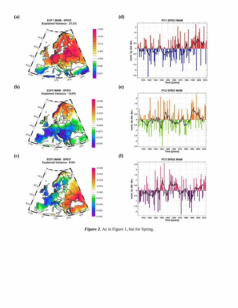
(a)
(d)
(b)
(e)
(c)
(f)
Figure 2. As in Figure 1, but for Spring.

(a)
(d)
(b)
(e)
(c)
(f)
Figure 3. As in Figure 1, but for Summer.

(a)
(d)
(b)
(e)
(c)
(f)
Figure 4. As in Figure 1, but for Autumn.

(a)
(d)
(b)
(e)
(c)
(f)
Figure 5. a) The composite map (High – Low) between the winter PC1 and winter Z850 (shaded) and
the wind vectors at 850mb (arrows);
b) As in Figure 5a, but for winter PC2;
c) As in Figure 5a, but for winter PC3;
d) The composite map (High – Low) between the winter PC1 and global winter SST;
e) As in Figure 5d, but for winter PC2;
f) As in Figure 5d, but for winter PC3;
(The dotted areas indicate the Z500 and SST normalized anomalies significant at 95 % significance level on a
standard t-test).
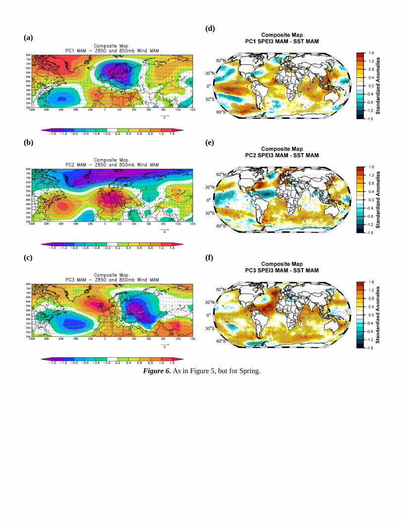
(a)
(d)
(b)
(e)
(c)
(f)
Figure 6. As in Figure 5, but for Spring.

(a)
(d)
(b)
(e)
(c)
(f)
Figure 7. As in Figure 5, but for Summer.

(a)
(d)
(b)
(e)
(c)
(f)
Figure 8. As in Figure 5, but for Autumn.

(a)
(d)
(g)
(b)
(e)
(h)
(c)
(f)
(i)
Figure 9. a) The correlation maps between winter PC1 and winter wet days (WET);
b) The correlation maps between winter PC2 and winter wet days (WET);
c) The correlation maps between winter PC3 and winter wet days (WET);
d) The correlation maps between winter PC1 and winter Cloud Cover (CLD);
e) The correlation maps between winter PC2 and winter Cloud Cover (CLD);
f) The correlation maps between winter PC3 and winter Cloud Cover (CLD);
g) The correlation maps between winter PC1 and winter Soil Moisture (SOIL);
h) The correlation maps between winter PC2 and winter Soil Moisture (SOIL);
i) The correlation maps between winter PC3 and winter Soil Moisture (SOIL);
The dotted areas indicate the areas where the correlation coefficient is significant at 95 % significance level.
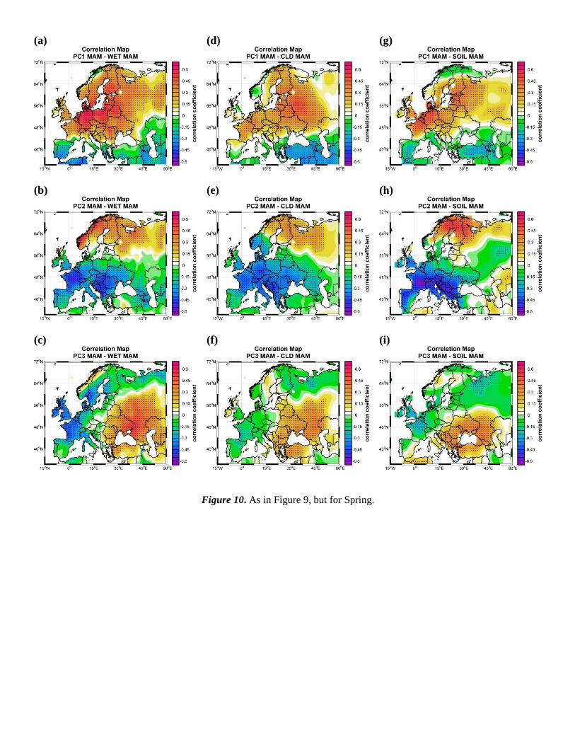
(a)
(d)
(g)
(b)
(e)
(h)
(c)
(f)
(i)
Figure 10. As in Figure 9, but for Spring.

(a)
(d)
(g)
(b)
(e)
(h)
(c)
(f)
(i)
Figure 11. As in Figure 9, but for Summer.

(a)
(d)
(g)
(b)
(e)
(h)
(c)
(f)
(i)
Figure 12. As in Figure 9, but for Autumn.

Table 1. The explained variance of the first ten seasonal EOFs. The EOFs highlighted in red, are
the seasonal EOFs used in this study.
Explained variance (%)
No. EOF Winter Spring Summer Autumn
EOF1 21.2 21.2 612.0 15.0
EOF2 13.6 14.0 4.69.4 12.2
EOF3 8.8 8.6 8.6 8.8
EOF4 5.7 5.1 6.3 6.5
EOF5 4.0 3.8 4.6 4.0
EOF6 3.7 3.0 4.1 3.3
EOF7 3.5 2.9 3.5 3.2
EOF8 3.3 2.0 2.8 2.6
EOF9 2.0 1.9 2.4 2.5
EOF10 1.9 1.8 2.0 2.0

Table 2. Teleconnection indices used in this study, time period and their source
Name Explanation Period Data source
AMO Atlantic Multidecadal
Oscillation
1950-2012 http://climexp.knmi.nl/data/iamo_hadsst2.dat
NAO North Atlantic
Oscillation
1950-2012 http://www.cru.uea.ac.uk/cru/data/nao.htm
AO Arctic Oscillation 1950-2012 http://www.atmos.colostate.edu/ao/Data/ao_index.html
SCA Scandinavian Pattern 1950-2012 http://www.cpc.noaa.gov/data/teledoc/scand.shtml
EAWR East Atlantic/ Western
Russia
1950 - 2012 http://www.cpc.ncep.noaa.gov/data/teledoc/eawruss.shtml
EA East Atlantic 1950 - 2012 http://www.cpc.ncep.noaa.gov/data/teledoc/ea.shtml
Niño 3.4 Niño 3.4 index 1950 - 2012 http://iridl.ldeo.columbia.edu/SOURCES/.Indices/.nino/.KAPLAN/
Niño 4 Niño4 index http://iridl.ldeo.columbia.edu/SOURCES/.Indices/.nino/.KAPLAN/
POL Polar/Eurasia 1950 - 2012 http://www.cpc.ncep.noaa.gov/data/teledoc/poleur.shtml
PDO Pacific Decadal
Oscillation
1950 - 2012 http://jisao.washington.edu/pdo/
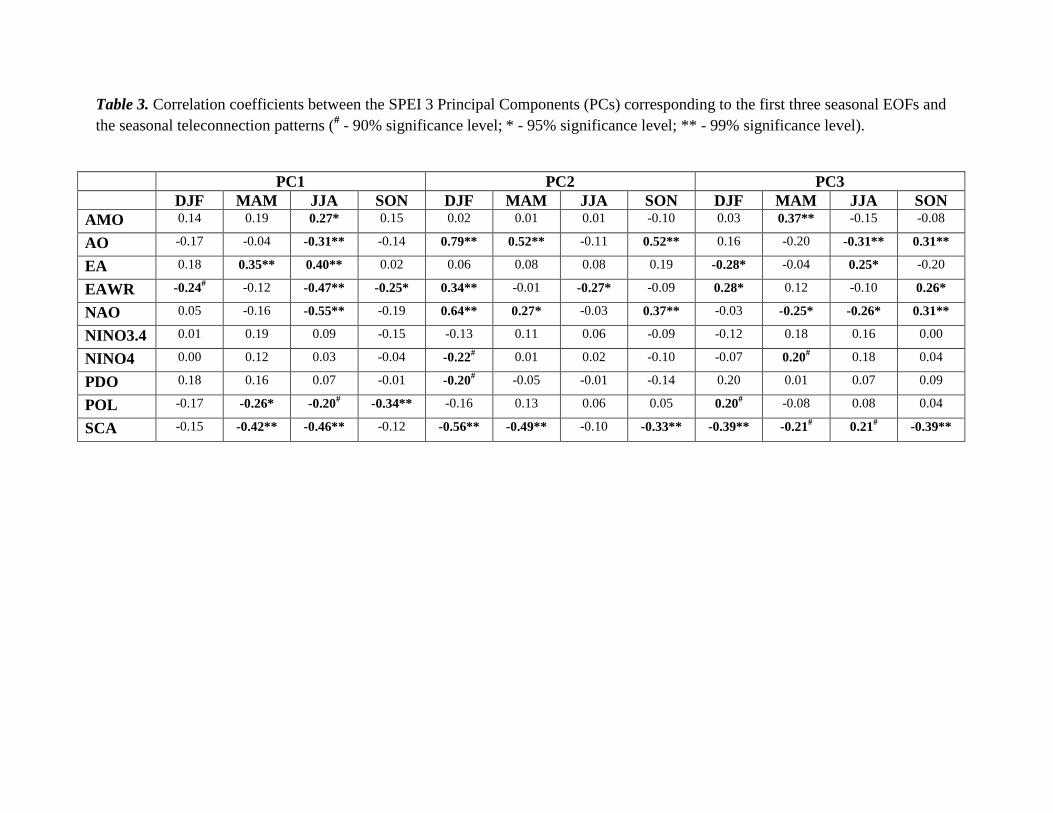
Table 3. Correlation coefficients between the SPEI 3 Principal Components (PCs) corresponding to the first three seasonal EOFs and
the seasonal teleconnection patterns (# - 90% significance level; * - 95% significance level; ** - 99% significance level).
PC1 PC2 PC3
DJF MAM JJA SON DJF MAM JJA SON DJF MAM JJA SON
AMO 0.14 0.19 0.27* 0.15 0.02 0.01 0.01 -0.10 0.03 0.37** -0.15 -0.08
AO -0.17 -0.04 -0.31** -0.14 0.79** 0.52** -0.11 0.52** 0.16 -0.20 -0.31** 0.31**
EA 0.18 0.35** 0.40** 0.02 0.06 0.08 0.08 0.19 -0.28* -0.04 0.25* -0.20
EAWR -0.24# -0.12 -0.47** -0.25* 0.34** -0.01 -0.27* -0.09 0.28* 0.12 -0.10 0.26*
NAO 0.05 -0.16 -0.55** -0.19 0.64** 0.27* -0.03 0.37** -0.03 -0.25* -0.26* 0.31**
NINO3.4 0.01 0.19 0.09 -0.15 -0.13 0.11 0.06 -0.09 -0.12 0.18 0.16 0.00
NINO4 0.00 0.12 0.03 -0.04 -0.22# 0.01 0.02 -0.10 -0.07 0.20
# 0.18 0.04
PDO 0.18 0.16 0.07 -0.01 -0.20# -0.05 -0.01 -0.14 0.20 0.01 0.07 0.09
POL -0.17 -0.26* -0.20#
-0.34** -0.16 0.13 0.06 0.05 0.20# -0.08 0.08 0.04
SCA -0.15 -0.42** -0.46** -0.12 -0.56** -0.49** -0.10 -0.33** -0.39** -0.21# 0.21
# -0.39**
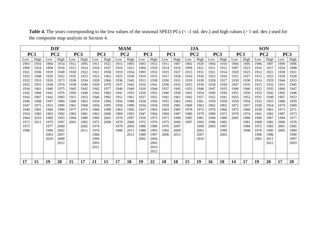
Table 4. The years corresponding to the low values of the seasonal SPEI3 PCs (< -1 std. dev.) and high values (> 1 std. dev.) used for
the composite map analysis in Section 4.
DJF MAM JJA SON
PC1 PC2 PC3 PC1 PC2 PC3 PC1 PC2 PC3 PC1 PC2 PC3 Low High Low High Low High Low High Low High Low High Low High Low High Low High Low High Low High Low High
1903
1909
1921
1925
1932
1933
1934
1942
1943
1946
1947
1949
1954
1964
1972
1973
1996
1916
1924
1936
1948
1953
1955
1961
1966
1967
1968
1975
1981
1982
2010
2011
1904
1908
1919
1920
1926
1938
1940
1941
1942
1947
1953
1960
1963
1969
1970
1977
1996
2003
2010
1914
1918
1949
1952
1973
1974
1975
1976
1983
1984
1989
1990
1992
1993
1997
2000
2002
2007
2008
2012
1912
1915
1930
1935
1936
1939
1945
1950
1951
1960
1961
1977
1983
1994
2001
1905
1914
1922
1923
1934
1940
1942
1948
1953
1963
1968
1976
1981
1989
1992
2002
2011
1911
1918
1921
1923
1928
1929
1942
1943
1946
1954
1956
1960
1963
1969
1972
1974
1976
1984
1996
2003
2011
1922
1937
1958
1962
1966
1970
1977
1983
1992
1994
1995
1998
2000
2001
2008
1915
1916
1919
1923
1936
1937
1940
1941
1951
1956
1958
1963
1969
1970
1978
1979
1980
1903
1921
1934
1938
1943
1945
1949
1953
1961
1989
1990
1992
1993
1997
2000
2003
2011
2012
1903
1904
1905
1910
1913
1916
1918
1920
1927
1928
1934
1937
1947
1950
1972
1986
1988
1989
2002
1915
1929
1932
1933
1938
1941
1944
1953
1955
1956
1958
1963
1964
1973
1976
1980
1993
1997
2004
2005
2010
2012
1911
1914
1915
1917
1930
1936
1937
1940
1941
1955
1959
1963
1969
1971
1975
1976
1992
2006
1907
1916
1927
1928
1931
1935
1945
1958
1961
1962
1981
1985
1987
1998
2000
2007
2009
2012
1902
1909
1913
1916
1919
1925
1933
1941
1942
1945
1969
1978
1980
1985
1997
1920
1921
1931
1936
1938
1939
1946
1954
1957
1961
1963
1972
1979
1981
1992
1999
2002
2007
2010
1904
1911
1921
1923
1928
1934
1947
1949
1952
1959
1962
1976
1989
1994
1996
2003
1910
1912
1914
1926
1927
1930
1933
1936
1941
1958
1965
1966
1972
1980
1985
1997
1999
2002
1904
1907
1920
1921
1939
1947
1949
1951
1955
1959
1972
1975
1976
2005
1905
1923
1925
1927
1930
1935
1940
1950
1952
1954
1957
1960
1974
1980
1981
1984
1998
1906
1910
1912
1913
1914
1915
1922
1925
1931
1933
1936
1939
1941
1960
1968
1972
1976
1996
2002
1907
1917
1921
1923
1929
1932
1935
1942
1948
1953
1954
1961
1962
1967
1982
1983
1985
1986
2011
2012
1909
1924
1938
1939
1944
1951
1960
1965
1967
1968
1974
1975
1987
1994
2000
2001
2005
1906
1908
1921
1928
1933
1945
1947
1948
1953
1959
1969
1971
1973
1977
1978
1985
1989
1990
1997
2003
17 15 19 20 15 17 21 15 17 18 19 22 18 18 15 19 16 18 14 17 19 20 17 20