1

Seasonal Variation of Inorganic Nutrients (DSi, DIN and DIP) Concentration in Swedish River

By

Rafiq Ahmed (rafiq353@yahoo.com)

Supervisor Åsa Danielsson

Water Resources and Livelihood Security Programme, Linköping University, SE-581 83 Linköping, Sweden.

2

Abstract Rivers have been playing most important role as fresh water source and medium of nutrient transportation from terrestrial to aquatic ecosystem. Inorganic form of nutrients (DSi, DIN and DIP) are plant available mostly control the productivity of aquatic ecosystem. Transfer of these nutrients in higher concentrations cause harmful eutrophication in receiving water body. Study of dissolved inorganic nutrients concentrations in 12 Swedish rivers of different basin characteristics demonstrated both similar and varying behaviour from river to river and from season to season depending on catchment hydrology; land use and geology. Highest concentration did not coincide with the highest runoff. High DSi concentration observed in the unperturbed rivers however, high DIN and DIP concentration observed in agriculture dominated river followed by river basin dominated by industrial and urban activities. DSi and DIN concentration observed high in winter and decreased through spring to reach lowest in summer. DIP concentration although found low in summer but high concentration observed in early spring and early autumn. Rivers with low average runoff positively correlated with DSi and DIN concentration however, DIP demonstrated weak correlation.

3

Acknowledgements

I wish to express my profound gratitude to my supervisor Åsa Danielsson, Department of Water and Environmental Studies, for her motivations, guidance and untiring contributions all through this work. I am also grateful to Dr Juile Wilk, Lars Rahm, Björn Ola Linner and all other teachers of Department of Water and Environmental Studies, for their generous help during course work. I would like to thank all of my class friends specially Mohammad Abu Quwsar for his encouragement. I would also like to be thankful to my family members and friends for their unconditionally support, who are living in Bangladesh. Finally, I would like to dedicate this paper to my father who always initiates me positive ways of life.

4

Table of Contents Table of Contents………………………………………………………………………………4 List of Tables…………………………………………………………………………………...5 List of Figures………………………………………………………………………………….5 Appendix……………………………………………………………………………………….5 1. Introduction………………………………………...………………......................................6 1.1 Aim of the study………………...…………………………………………………..…...7 1.2. Objective of the study…………………………………………………………………..7 2. Background………………………………...…………………………………………..........7 2.1. Nutrient introduction to aquatic ecosystem…..…...…………………………..….........10 2.2. Problems of nutrient over enrichment and composition change……………….…..….11 2.3. Sources of nutrients……………………………………………………..…...…….......11 2.3.1. Phosphorous.………………………………….…………………….……………..12 2.3.2. Nitrogen….………………………………………………...………………………13 2.3.3. Silica......…………… …………………………………………………….……….14 3. Data materials and method…………………………………………………………………15 3.1. Sources of data….……………………………………………………………..………15 3.2. Stepwise regression method…………...………………………………………………15 3.3. Correlation method…………………………………………………………………….16 4. General characteristics of studied rivers and catchments…….……………………...……..17 5. Results………………………………………………………………………...……………22 5.1. Descriptive statistics…………………………………………………………..………22 5.1.1Yearly variation in nutrients concentrations………………………………………..24 5.1.2 Monthly variation in nutrients concentrations……………………………………..31 5.2 Regression analysis……………………………………………….………..…………..40 6. Discussion……………………………………………………………………….………....42 6.1. Dissolved silica (DSi)……..…………………………………………….…………….42 6.2. Dissolved inorganic nitrogen (DIN)……. ……............................................………....44 6.3 Dissolved inorganic phosphate (DIP)…… ………………………….……..………….46 6.4. Differences and similarities...… ………………………………………………………47 7. Conclusion……………………………………………….........................................……...48 8. References………………………………………………………………………………….49

5

List of Tables Table 1: Mean Runoff, DSi, Total N, Total P, DIN and DIP of 12 Swedish rivers from 1984 to 2005(Runoff 1985 to 2000)……….…………………………….23 Table 2: Showing coefficients of regression model for DSi concentrations and R2 (adj) value(n.s. =non-significant, α=0.05)………………………………………………………….40 Table 3: Showing coefficients of regression model for DIN concentrations and R2 (adj) value (n.s. =non-significant, α=0.05)…………..…………………………………………………....41 Table 4: Showing coefficients of regression model for DIP concentrations and R2 (adj) value (n.s. =non-significant, α=0.05)…..……….…………………………………………………...41

List of Figures Figure 1: Schematic representation of the phosphorus cycle (Source: www.lenntech.com)... 13 Figure 2: Nitrogen cycle (source: physicalgeography.net).……...………………...…………14 Figure 3: Map showing the sampling site of the studied rivers (Source: www.slu.se)……….18 Figure 4: Map showing land use of the study area (Source: http://maps.grida.no/baltic/).......19 Figure 5: Map showing population density of the study area (Source:http://maps.grida.no/baltic/).........................................................................................20 Figure 6:(a-l) Showing yearly variation in DSi (mg/l) concentration with runoff (10PP

7PPmPP

3PP -

10PP

9PPmPP

3PP)…………………………………………………........................................................... 25

Figure 7 :( a-l) Showing yearly variation in DIN concentration (µg/l) with runoff (10 PP

6PPmPP

3 PP-

10 PP

7PPmPP

3PP)…………………………………………………………………………………………27

Figure 8 :( a-l) Showing yearly variation in DIP concentrations (µg/l) with runoff (10 PP

7PPmPP

3PP -

10PP

9PPmPP

3PP)…………………………………………………………………………………………29

Figure 9 :( a-l) Showing monthly DSi concentrations variation in studied rivers…………....32 Figure 10 :( a-l) Showing monthly DIN concentrations variation in studied rivers………….34 Figure 11 :( a-l) Showing monthly DIP concentrations variation in studied rivers……..……36 Figure 12 :( a-l) Showing monthly runoff variation in studied rivers………...………………38

Appendix Appendix A: Correlation between yearly average runoff and inorganic- nutrients (DSi, DIN and DIP)……………………………………………………………..57 Appendix B: Correlation between monthly average runoff and inorganic nutrients-

(DSi, DIN and DIP)…………………………………………………………………..…….57 Appendix C: Graph showing residual analysis of DSi……………………………………….58 Appendix D: Graph showing residual analysis of DIN……………………………………....60 Appendix E: Graph showing residual analysis of DIP……………………………………….62

6

1 Introduction Rivers have always been one of the most important freshwater resources and most developmental activities are depended upon the availability of fresh water. Fresh water is being used in multiple purposes of development like in agriculture, industry, transportation, aquaculture, public water supply etc. However, since earlier, rivers have also been used for cleaning and dumping of various development activities. Huge loads of waste from industries, domestic sewage, agricultural activities and managed forests, as well as natural background losses and atmospheric deposition discharge into rivers, resulting in large scale deterioration of the water quality. The growing problem of degradation of river ecosystem has necessitated the monitoring of water quality of various rivers all over the world to evaluate their production capacity, utility potential and to plan restorative measures. Rivers play important role in worldwide delivery of nutrients from terrestrial ecosystem to the coastal water which causes higher nutrient concentrations and subsequent harmful eutrophication problems in the aquatic ecosystem (Nixon, 1996). The water quality of natural rivers depends on the character of the upstream of the drainage basin, which profoundly influences the chemistry of water mainly through the anthropogenic activities .The worldwide growth in population and resulted increased demand for water, energy and land use exacerbated the situation. Excessive landscape disturbance by human activities at the catchment areas alter the rates of weathering, leaching and erosion by removing vegetative cover, exposing soil, and increasing water runoff velocity. Agricultural chemicals, urban wastewater, industrial waste, emissions from vehicles, fossil fuel-burning electric apparatus and other sources produce a variety of compounds that affect water chemistry by discharging nutrients such as nitrogen and phosphorous . Nitrogen, phosphorous and silica are the three important elements (nutrients) most likely to control the productive function of aquatic ecosystems. Various climatological and anthropogenic factors by controlling water discharge govern the flux and hence concentrations of nutrients in the water body. Variations observed in river flows depend on the precipitation in its reception areas which depend on seasonal cycle of the year. After entrance in the drainage basin, the part of the water which does not go back to atmosphere through evapotranspiration can reach the aquatic system by overland, through and groundwater base flow. In its pathway from land to the river through the soil-rock complex carries everything that can be mobilized by its physical or chemical action, including the soluble and particulate products which is the result of interaction with the organisms (Silva et al., 2001). Rivers along the Baltic Sea by discharging nutrients and other chemical elements from their basin deteriorated the water quality to a grater extent. During the second half of the last century nitrogen and phosphorous load in the Baltic Sea increased four and eight times respectively due to increased population, agricultural and industrial activities in the drainage area (Larsson et al.,1985 ).These increased nutrients load deteriorated the water quality by increasing algal bloom, lowering light penetration, transformed benthic zone anoxic and lifeless (SIBER, 2002).While loads N and P increased but Si decreased which changed the phytoplankton composition of the water body (Danielsson et al., 2006). Two possible causes of DSi decrement are the rapid sinking of diatoms after the blooms and increase retention time of the water in the regulated water (SIBER, 2002). Anthropogenic activities at the catchment area tend to increase the discharge of N and P but reduce the supply of Si to the sea, which by altering concentration and the ratio of nutrients

7

may cause the shift of primary producer of the aquatic ecosystem from diatom to non-diatom species (Hecky and Kilham, 1988). The sources N, P and Si and their fate during travel from sources to the sea vary significantly with climate, hydrological regime and anthropogenic activities in the watershed (Billen and Garnier, 2007),causing the concentrations of nutrients to vary considerably from year to year and even from season to season. During the periods of high runoff nutrients are abundantly leached from soil increasing the loads and hence concentrations originating from diffuse sources and natural leaching. DIN usually increases during the early spring season from snowmelt runoff from watershed which cause spring bloom in most water body. Concentrations normally decrease during summer season as nutrients are taken up by phytoplankton and ultimately deposited to the bottom after death. 1.1 Aim of the study Aim of this present study is to observe– How concentrations of nutrients varied within a year due to change in hydrological regime with seasons -winter, spring, summer and autumn. It will enable us to know how climatological factors by controlling hydrological regime control the nutrient concentration in different rivers, and to predict how the concentrations of these nutrients may change as functions of runoff and seasons. Long term variation in concentrations of dissolved inorganic nutrients (DSi, DIN and DIP) in 12 Swedish rivers and its relation with runoff for the periods of 1985 to 2005. Study of long term variation in nutrient concentration of river would enable us to know concentration of which nutrient element increasing or decreasing with time and how it relates with runoff variation. 1.2 Objective of the study Objective of this study is to observe how dissolved inorganic nutrient concentrations (DSi, DIN and DIP) of twelve Swedish rivers of different basin characteristics, ranging from pristine river in north to agriculture dominated southern changing with time. And to which extent concentrations of the DSi, DIN and DIP controlled by the runoff which is also function of various climatological factors like- seasons. How different land use, population density, weathering rate and geological factors of the basins determining specific leakage of nutrients element control the relation between runoff and concentration. 2. Background Various studies (e.g. Beaulac and Reckhow, 1982; Frink, 1991; Jordan et al., 1997) have showed that land use strongly influence the nutrient discharges from land to the river. Differences in geological and climatic condition also control the nutrient discharge. Uses of fertilizers in intensive agriculture and urbanisation due to increased population resulted in increased sewage emission and use of detergents which increased the concentrations of dissolved nitrogen (N) and phosphorous (P) in the most of the world river over the last several decades. Loss of nitrogen and phosphorus from land is one of the major problems affecting water quality of Swedish river and resulting in eutrophication of the surrounding seas (Brandt and Ejhed, 2003). This problem is more pronounced in the agriculture-dominated southern part of

8

the country than the north where nutrient leaching from arable land is the main diffuse contributor to rivers comprises 97% of N and 90% of P and in central part the corresponding figures have been estimated to be 60–70% for N and P (Brandt and Ejhed, 2003).Use of fertilizer in Swedish agriculture, especially phosphorous, was doubled from 1920-1970 which increased phosphorous discharge to the water body to a greater extent (SEPA, 2002). Various farm facilities like dairies, as well as from scattered rural households whose wastewater is not connected to sewerage line or not processed by tertiary treatment facilities also contributing phosphorous to the nearby rivers and lakes. Although various activities and regulations, including tax on fertilizer use have again been brought down to the pervious level however, stored phosphorous in arable land remain undiminished. Extent of nutrient export from catchment area to river controlled mainly by the amount of water discharge, which is a function of climate, water retention capacity of soils, geologic structure and topographic relief of the basin. Before reaching nutrient at the mouth of the river there are a complex function of various physical, chemical and biological processes take place in the upstream basin and its way to river mouth. Processes like denitrification, assimilation by algae and aquatic macrophytes, adsorption onto stream bed sediments and sedimentation determine the loss of nutrients in the surface water during transport. Rivers in turn supply nutrients to the coastal seas which is most important parts of the world’s ecosystem and despite their small areas found valuable than open ocean and terrestrial system mostly due to the having capacity of storage and recycling of nutrients (Jickell, 1998). Nutrient input to the coastal zone via rivers increased by a factor of 2 to 3 globally due to the anthropogenic activities over the watershed and regions like northern Europe and parts of northern America showed much larger increase than the global (Duce et al., 1991). Inputs of N, P and Si by river and eutrophication of coastal water are inter-related. Due to changes in the riverine inflow of nutrients the frequency of eutrophication events has increased in various coastal water over the last decades. Evidence of such bloom of noxious phytoplankton observed in the Dutch Wadden Sea (Smayda, 1990) and hypoxia reported in river dominant coastal water like Chesapeake Bay (Officer et al., 1984) and some areas of the Baltic Sea (Andersson & Rydberg, 1988). Transportation of nutrients from sources through the river controlled by the various human induced activities in its way to coastal water. Presence of dams along the river affects the transportation of nutrients by causing artificial lake affect (Humborg et al., 1997). As the number of dams increasing worldwide for electricity generation or protection from flood, transportation of sediment hence transportation of phosphorous and silica to the coastal water are decreasing (Halim, 1991). Basins of the northern Sweden rivers are sparsely populated and agriculture activities almost absent or very low but dams are the most obvious human impact which decreased DSi discharge. Dams on Lule river for electricity generation has increased Si retention rate by 698 tonnes/year which resulted in increased diatom production in Störa Lulevatten and this increased retention corresponds to a reduction in the Si transport to the Gulf of Bothnia by 2%(Drugge, 2003). In Danube River damming caused as high as 50% reduction of DSi concentrations (Humborg et al., 1997). Phosphorous species which is carried by the rivers to the coastal water are mostly in particulate form (Howarth et al., 1996; Froehlich, 1988) also affected by the retention process way to the sea. Besides artificial lake affect of dams, presence of lakes along the river basin cause low riverine load compare to the other basin not having lakes in its drainage basin (Grimvall & Stålnacke, 2001). In Sweden and Finland a large number of lakes in the

9

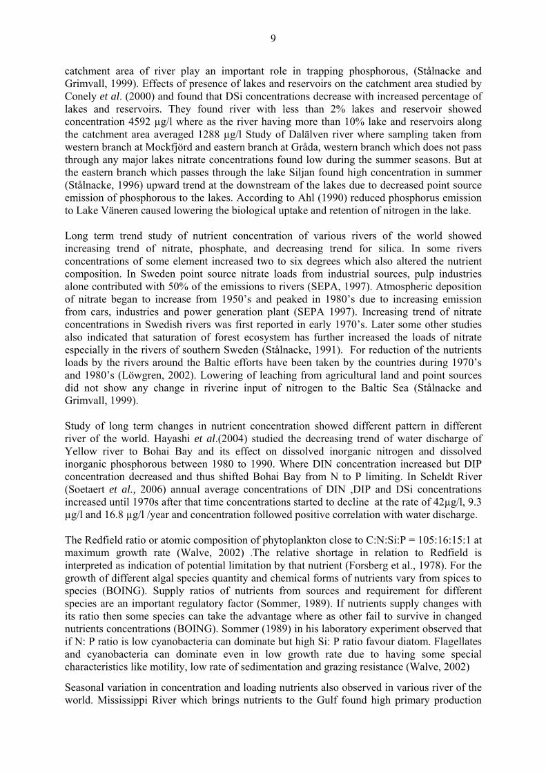
catchment area of river play an important role in trapping phosphorous, (Stålnacke and Grimvall, 1999). Effects of presence of lakes and reservoirs on the catchment area studied by Conely et al. (2000) and found that DSi concentrations decrease with increased percentage of lakes and reservoirs. They found river with less than 2% lakes and reservoir showed concentration 4592 µg/l where as the river having more than 10% lake and reservoirs along the catchment area averaged 1288 µg/l Study of Dalälven river where sampling taken from western branch at Mockfjörd and eastern branch at Gråda, western branch which does not pass through any major lakes nitrate concentrations found low during the summer seasons. But at the eastern branch which passes through the lake Siljan found high concentration in summer (Stålnacke, 1996) upward trend at the downstream of the lakes due to decreased point source emission of phosphorous to the lakes. According to Ahl (1990) reduced phosphorus emission to Lake Väneren caused lowering the biological uptake and retention of nitrogen in the lake. Long term trend study of nutrient concentration of various rivers of the world showed increasing trend of nitrate, phosphate, and decreasing trend for silica. In some rivers concentrations of some element increased two to six degrees which also altered the nutrient composition. In Sweden point source nitrate loads from industrial sources, pulp industries alone contributed with 50% of the emissions to rivers (SEPA, 1997). Atmospheric deposition of nitrate began to increase from 1950’s and peaked in 1980’s due to increasing emission from cars, industries and power generation plant (SEPA 1997). Increasing trend of nitrate concentrations in Swedish rivers was first reported in early 1970’s. Later some other studies also indicated that saturation of forest ecosystem has further increased the loads of nitrate especially in the rivers of southern Sweden (Stålnacke, 1991). For reduction of the nutrients loads by the rivers around the Baltic efforts have been taken by the countries during 1970’s and 1980’s (Löwgren, 2002). Lowering of leaching from agricultural land and point sources did not show any change in riverine input of nitrogen to the Baltic Sea (Stålnacke and Grimvall, 1999). Study of long term changes in nutrient concentration showed different pattern in different river of the world. Hayashi et al.(2004) studied the decreasing trend of water discharge of Yellow river to Bohai Bay and its effect on dissolved inorganic nitrogen and dissolved inorganic phosphorous between 1980 to 1990. Where DIN concentration increased but DIP concentration decreased and thus shifted Bohai Bay from N to P limiting. In Scheldt River (Soetaert et al., 2006) annual average concentrations of DIN ,DIP and DSi concentrations increased until 1970s after that time concentrations started to decline at the rate of 42µg/l, 9.3 µg/l and 16.8 µg/l /year and concentration followed positive correlation with water discharge. The Redfield ratio or atomic composition of phytoplankton close to C:N:Si:P = 105:16:15:1 at maximum growth rate (Walve, 2002) .The relative shortage in relation to Redfield is interpreted as indication of potential limitation by that nutrient (Forsberg et al., 1978). For the growth of different algal species quantity and chemical forms of nutrients vary from spices to species (BOING). Supply ratios of nutrients from sources and requirement for different species are an important regulatory factor (Sommer, 1989). If nutrients supply changes with its ratio then some species can take the advantage where as other fail to survive in changed nutrients concentrations (BOING). Sommer (1989) in his laboratory experiment observed that if N: P ratio is low cyanobacteria can dominate but high Si: P ratio favour diatom. Flagellates and cyanobacteria can dominate even in low growth rate due to having some special characteristics like motility, low rate of sedimentation and grazing resistance (Walve, 2002)

Seasonal variation in concentration and loading nutrients also observed in various river of the world. Mississippi River which brings nutrients to the Gulf found high primary production

10

during February to July (Justic et al., 1993). However, hypoxia observed during the summer due to decomposition of organic matter accumulated during spring phytoplankton bloom (Qureshi, 1995). Seasonal variation in nutrient (DIP and DIN) loads observed in the Bangpakong estuary, Thailand ( Buranapratheprat et al.,2002) where high loading observed in September and concentration did not coincide with loading .High concentration found few months before the high loading in September which was mostly due to seasonal variations in residence times and loadings. Nutrient concentrations of Bandon River, southwest Ireland, showed temporal and spatial variation. In case of Nitrate highest concentrations 1694 µg/l observed in winter (November) at the upstream and lowest 3.22 µg/l in summer at the mouth of the estuary. Phosphate and DSi concentration also followed same seasonal variation and concentrations both nutrients found as low as 0.28 µg/l at the river mouth in summer (in August and July respectively). These changes in concentrations with time and space alter the Redfield ratio (N: P) which was higher at the upstream but decreased to 10 at the river mouth (Muylaert, 1999). Nutrient concentrations of Boise River from 1989 to 1999 showed variation between upstream and downstream. Concentrations of total P found 100µg/l at near diversion dam to 1300 µg/l at other part of the river. Concentration also followed seasonal pattern with low concentrations in winter when water flow was low. DIP which comprises 75% to 80% of the total P also followed similar pattern with respect to locations and flow condition (IDEQ, 2001). 2.1 Nutrient introduction to aquatic ecosystem Nutrients enter to the aquatic ecosystem through various processes; combination of chemical and physical processes with water movement determines the introduction of nutrients to the water body. As nutrients remain in different chemical forms, the various processes of water transport provide a range of impacts on nutrient transfer. Introduction to the water body occur mainly through precipitation, groundwater flow and surface water runoff. Anthropogenic sources like intensive agricultural, urban sewerage and livestock sewage bring a large quantity of nutrient to aquatic environment. Soil erosion is the most important mechanism which transfers nutrients like nitrogen and phosphorous from terrestrial environment to aquatic environment. Cultivation, overgrazing and clear cutting also accelerates the rate of nutrient transfer (Dugdale et al., 1998). Vertical movement of nutrient from agricultural and other places where nutrient level is high through leaching transport soluble nutrients from surface soil profile to ground water and then laterally transfer to lakes, rivers and oceans. Atmospheric input of nutrients specially nitrogen which mostly increase due to human activities. Input by this way through wet and dry deposition of elements which liberated to the atmosphere through burning of fossil fuel, intensive agricultural and from farming practices like poultry, dairy and pig farming. Biological process like N fixation by phytoplankton also brings atmospheric nitrogen to the aquatic ecosystem. Lateral water flow also brings organisms from one ecosystem to another ecosystem and organisms facing mortality release nutrient to that ecosystem. Weathering from geological sources, although this process is slow and transfer very small quantities but play vital role in sustaining important nutrient element like P, Fe and Si in natural ecosystem(Dugdale et al.,1998). Flux through weathering processes depend on nature

11

and composition of bed rocks and its interaction with climatological factors. Usually weathering rate decrease with age of weathering surface but acid deposition from anthropogenic sources accelerate weathering rate. 2.2 Problems of nutrient over enrichment and composition change Coastal waters are the most important and productive and economically vital ecosystem for any country however, it is the most heavily loaded ecosystem of the Earth. Activities in catchment area produce large quantities of nutrients which exported finally to the coastal water by rivers and streams. Concentrations of nutrients are usually higher at the mouth of the river (estuary) where mixing of fresh and saline water take place and movement is low and water is rich in various organisms. Most of the estuaries are now a days showing eutrophication with some variation in scale, intensity and impact (Bricker et al., 1999). Water exchange rate with open ocean is important factor in maintaining the ecosystem quality. Low exchange with open ocean increase the residence time of water as well as nutrient which make the coastal water vulnerable, Baltic Sea is one of the examples of such areas. Primary productivity of any water body depends on various factors like availability of light, nutrients, grazing, mortality and other physical factors. Interplay among these factors will determine how the water body responds to the nutrient loadings. Although productivity of any ecosystem mostly controlled by the nutrient, excess or lack of one or more nutrient element can adversely affect the aquatic ecosystem. Usually phytoplankton blooms occur only when plankton turnover time is shorter than the water residence time. If water residence time less than turnover time of phytoplankton then there is less possibility to be eutrophied. In some ecosystem moderate nutrient loading can be beneficial as increased primary production lead to increased fish production and harvest (Nixon, 1996). Other ecosystem like coral reefs can be damaged even small increase in nutrient loading. Nutrient from watershed bring various element at various ratio which ultimately change the nutrient concentrations and ratio of the receiving water body. Changed concentrations and ratios of nutrients due to the discharge from watershed affect the biodiversity of that water by promoting some species over other species. Ratio and concentrations change cause both economic and non economic loss like eutrophication and associated anoxia, hypoxia and dead bottom, loss of fishery resources, change in trophic and ecological structure, loss of biodiversity and impact the aesthetic use of water body. 2.3 Sources of nutrients Nutrients discharged to the rivers from various sources with in the catchment areas of the rivers. Sources include industries, municipal waste water treatment plants, rural scattered dwellings and losses from agriculture fields, managed forests, atmospheric deposition as well as natural background losses. All these sources are mainly divided into point and non-point sources. Of them although, point sources are comparatively easy to control but diffuse sources is difficult to both identify and quantify especially which are widespread and development of solutions for control measures also complicated. Among the various diffuse sources agriculture has long been a major source of nutrients all over the world. Nutrients are mainly derived from fertilisers used in agricultural field and, as well as effluent from huge pig, dairy farms and agro-industrial units. Nutrients discharge from non-point source starts usually with precipitation. During the period of high runoff leaching rate becomes high. When the resulting runoff of precipitation moves over and through the soil, it picks up and carries

12

away natural and anthropogenic nutrients, finally transporting them to streams, rivers, wetlands, lakes, and even to ground water. Lack of appropriate agricultural practices in some areas have polluted rivers and groundwater, to a greater extent by increasing soil erosion. Nowadays, many wetlands have been drained, and converted into cropland which also aggravated nutrient concentrations in many water bodies. Globally, about 40 percent of the inorganic nitrogen fertilizer applied to agricultural fields is volatilized as ammonia and lost to the atmosphere, either directly from fertilizer or from animal wastes. Combustion of fossil fuels, like coal and gasoline also transfer nitrogen to the atmosphere. Local contributions also come from evaporative losses of nitrogen in the vicinity of open-air manure and from cattle farming. This nitrogen later deposited onto the landscape as dry pollutants or acid rain (Howarth et al., 2000). Pollution Load compilations-4 by Helsinki Commission(2004) reported that diffuse source, mainly agriculture discharge 60% of waterborne nitrogen and 50% of phosphorous to the Baltic Sea. Although improved waste water treatment in industry and municipal waste water treatment plants have reduced from the point sources between 1985- 2004 but reduction from diffuse sources did not fulfil the target (HELCOM, 2005). In different countries various environmental laws are imposed to control point sources, which have resulted in reductions from point sources like industries and from the wastewater treatment plants. Although violations occur, in most cases, the legislation has had a positive influence on preventing or limiting contaminants from entering water systems. 2.3.1 Phosphorous Phosphorus is the eleventh-most abundant mineral in the earth's crust and has no gaseous state. The natural background levels of total phosphorus are generally less than 30µg/l. The natural levels of orthophosphate usually range from 5µg/l to 50 µg/l (Dunne and Leopold, 1978). Natural inorganic phosphorus deposits occur primarily as phosphate in the mineral apatite which found in igneous, metamorphic, and sedimentary rocks. When released into the environment, phosphate transformed to orthophosphate depending on the pH of the surrounding soil (Osmond et al., 1995). In case of point sources, sewage system provides most of the available phosphorus to surface water bodies and agriculture source is the largest diffuse source. Nowadays, introduction of sewage and industrial waste water treatment reduced emission form the point sources to a great extent. Usually during treatment of sewage primary treatment removes only 10% of the phosphorus in the waste; secondary treatment removes an additional 30%. Tertiary treatment which includes chemical precipitation and biological treatment remove additional phosphorous from waste water. Phosphate in soil is not readily available for uptake and it is rapidly immobilized as calcium or iron phosphates. Most of the phosphorus in soils is adsorbed to soil particles or incorporated into organic matter (Smith, 1990). Phosphorus travel to surface water attached to particles of soil or manure eroded by water and also can dissolve into runoff water as it passes over the surface of the agricultural field (Lory, 2007).

13

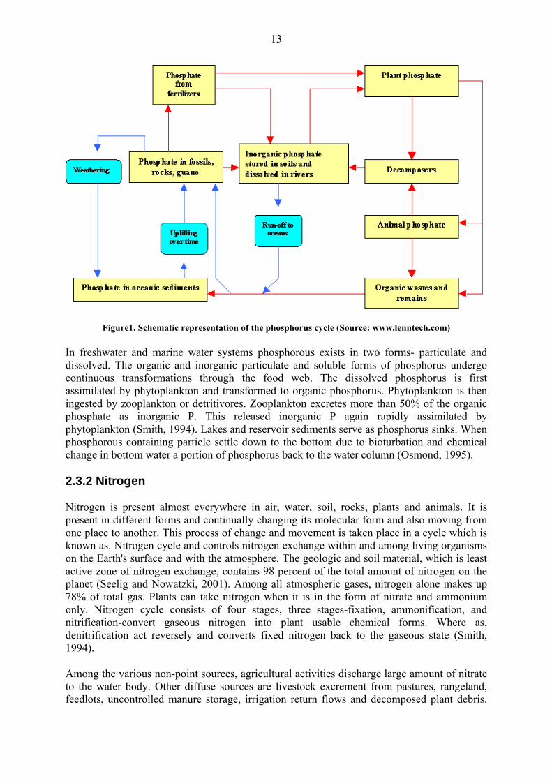
Figure1. Schematic representation of the phosphorus cycle (Source: www.lenntech.com) In freshwater and marine water systems phosphorous exists in two forms- particulate and dissolved. The organic and inorganic particulate and soluble forms of phosphorus undergo continuous transformations through the food web. The dissolved phosphorus is first assimilated by phytoplankton and transformed to organic phosphorus. Phytoplankton is then ingested by zooplankton or detritivores. Zooplankton excretes more than 50% of the organic phosphate as inorganic P. This released inorganic P again rapidly assimilated by phytoplankton (Smith, 1994). Lakes and reservoir sediments serve as phosphorus sinks. When phosphorous containing particle settle down to the bottom due to bioturbation and chemical change in bottom water a portion of phosphorus back to the water column (Osmond, 1995). 2.3.2 Nitrogen Nitrogen is present almost everywhere in air, water, soil, rocks, plants and animals. It is present in different forms and continually changing its molecular form and also moving from one place to another. This process of change and movement is taken place in a cycle which is known as. Nitrogen cycle and controls nitrogen exchange within and among living organisms on the Earth's surface and with the atmosphere. The geologic and soil material, which is least active zone of nitrogen exchange, contains 98 percent of the total amount of nitrogen on the planet (Seelig and Nowatzki, 2001). Among all atmospheric gases, nitrogen alone makes up 78% of total gas. Plants can take nitrogen when it is in the form of nitrate and ammonium only. Nitrogen cycle consists of four stages, three stages-fixation, ammonification, and nitrification-convert gaseous nitrogen into plant usable chemical forms. Where as, denitrification act reversely and converts fixed nitrogen back to the gaseous state (Smith, 1994). Among the various non-point sources, agricultural activities discharge large amount of nitrate to the water body. Other diffuse sources are livestock excrement from pastures, rangeland, feedlots, uncontrolled manure storage, irrigation return flows and decomposed plant debris.

14

Nitrogenous fertilizer used on lawn and garden also contribute some extent. Point sources are industrial use of nitrogen in manufacturing processes release nitrate in the effluent water. Nitrate is used in meat curing, production of fertilizer, heat-transfer fluid, explosives, glass, and heat-storage medium for solar-heating applications (Kubek et al., 1990).

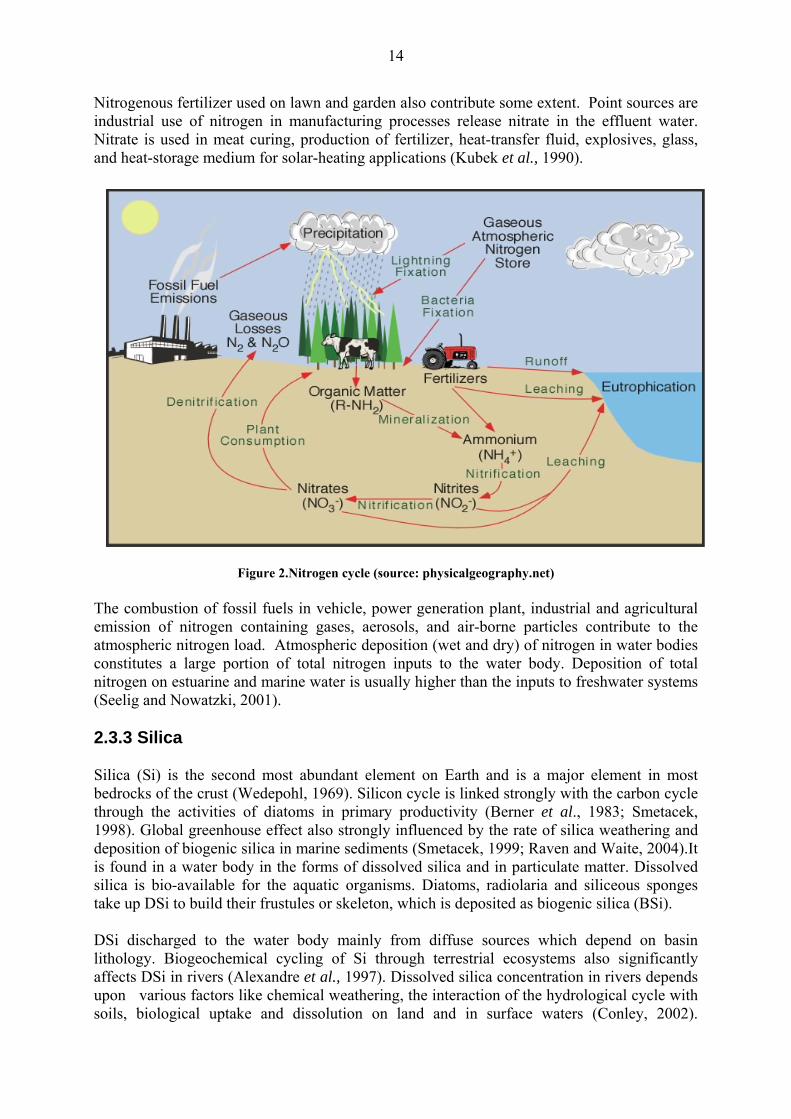
Figure 2.Nitrogen cycle (source: physicalgeography.net)

The combustion of fossil fuels in vehicle, power generation plant, industrial and agricultural emission of nitrogen containing gases, aerosols, and air-borne particles contribute to the atmospheric nitrogen load. Atmospheric deposition (wet and dry) of nitrogen in water bodies constitutes a large portion of total nitrogen inputs to the water body. Deposition of total nitrogen on estuarine and marine water is usually higher than the inputs to freshwater systems (Seelig and Nowatzki, 2001). 2.3.3 Silica Silica (Si) is the second most abundant element on Earth and is a major element in most bedrocks of the crust (Wedepohl, 1969). Silicon cycle is linked strongly with the carbon cycle through the activities of diatoms in primary productivity (Berner et al., 1983; Smetacek, 1998). Global greenhouse effect also strongly influenced by the rate of silica weathering and deposition of biogenic silica in marine sediments (Smetacek, 1999; Raven and Waite, 2004).It is found in a water body in the forms of dissolved silica and in particulate matter. Dissolved silica is bio-available for the aquatic organisms. Diatoms, radiolaria and siliceous sponges take up DSi to build their frustules or skeleton, which is deposited as biogenic silica (BSi). DSi discharged to the water body mainly from diffuse sources which depend on basin lithology. Biogeochemical cycling of Si through terrestrial ecosystems also significantly affects DSi in rivers (Alexandre et al., 1997). Dissolved silica concentration in rivers depends upon various factors like chemical weathering, the interaction of the hydrological cycle with soils, biological uptake and dissolution on land and in surface waters (Conley, 2002).

15

Weathering rates are controlled by the interactions of climate, geology and vegetation (Berner, 1992). Particulate biogenic silica in the form of phytoliths eroded from soils may also represent diffuse inputs of dissolved silica (Garnier et al., 2002). A very small portion of dissolved and amorphous silica discharged to the water body from point sources like – detergents, paper production process and in sewage inputs (Clark et al., 1992). 3. Data materials and methods 3.1 Sources of Data Monthly nutrients data of the rivers have been retrieved from the database of Department of Environmental Assessment at the Swedish University of Agricultural Sciences, SLU, (http://www.slu.se). Regular monitoring of nutrients and other major constituents in Swedish rivers began in 1965 and in the early 1970’s a National Monitoring Programme (PMK) covering all major Swedish rivers was established. Since then the core of the programme has remained practically unchanged. Data on water chemistry and vegetation cover collected within the frame of the integrated monitoring in Sweden. The water samples were collected monthly at the major river mouths, except some smaller rivers in areas dominated by agricultural activities where samples are taken every second week. It should be mentioned here that all water samples were taken at a depth of 0.5 m. The samples are taken directly into the bottles to avoid contamination and sent directly to SLU lab where they are analysed according to standard methods. Details analytical methods of DIN, DIP and DSi are available on- http://info1.ma.slu.se/ma/www_ma.acgi$Analysis?ID=AnalysisList Monthly runoff data were retrieved from the Swedish Meteorological and Hydrological Institute (SMHI). 3.2 Stepwise regression method Stepwise method combines both forward and backward procedures which is better in the exploratory phase of research or for purposes of pure prediction than theory testing (Menard, 1995). Due to intercorrelations, the variance explained by certain variables will change when new variables enter to the equation. Sometimes a variable that qualified to enter losses some of its predictive validity when other variables enter to the model. In this method the most correlated independent selected first, remove the variance in the dependent, then select the second independent variable which most correlates with the remaining variance in the dependent, and continue until selection of an additional independent does not increase the R-squared by a significant amount (usually significance = .05). Each independent variable is entered in sequence and its value assessed. If addition of the variable contributes to the model then it is retained, but all other variables in the model are then re-evaluated to see if they are still contributing to the improvement of the model. If independent variables no longer contribute significantly they are removed. Thus, this method ensure end up with the smallest possible set of independent variables included in model. The purpose of a multiple regression is to find equation, which best predict the concentrations of the inorganic nutrients for each river as a linear function of the independent variables. The model will help to predict concentrations of inorganic nutrients as a function of runoff and seasons.

16

The goodness-of-fit of the multiple regression models was evaluated by the adjusted RPP

2PP-value,

which is the approximation of the coefficient of determination adjusted for the number of added predictor variables. The level of significance was set to 5%.

Inorganic nutrients=b BB0BB+b BB1BB*runoff+bBB2BB*ZBB1 BB+b BB3BB*ZBB2 BB+b BB4BB*ZBB3 BB+bBB5BB*runoff*ZBB1 BB+b6*runoff*ZBB2BB+b7*runoff*ZBB3

Where, Inorganic nutrients (DSi, DIN or DIP) concentrations are the dependent variables b B0 B = Intercept b1= coefficient for runoff b2= coefficient for the winter season (ZB1B), ZB1 B=1, if winter ZB1 B=0, otherwise bBB3 BB= coefficient for the spring season (ZBB2BB), ZBB2 BB=1, if spring ZBB2 BB=0, otherwise bBB4 BB= coefficient for the summer season (ZBB3BB), ZBB3 BB=1, if summer ZBB3 BB=0, otherwise bBB5 BB= coefficient for the interaction of runoff and winter bBB6 BB= coefficient for the interaction of runoff and spring bBB7 BB= coefficient for the interaction of runoff and summer

3.3 Correlation method

The correlation is one of the most common and most useful statistics that describes the degree

of relationship between two variables. In Pearson's product-moment correlation coefficient

two variables -average dissolved inorganic nutrients (DSi, DIN and DIP) concentration and

average runoff were used to determine the relation between runoff and concentration of the

studied rivers. For conducting significance test level of significance was fixed to α=0.05The

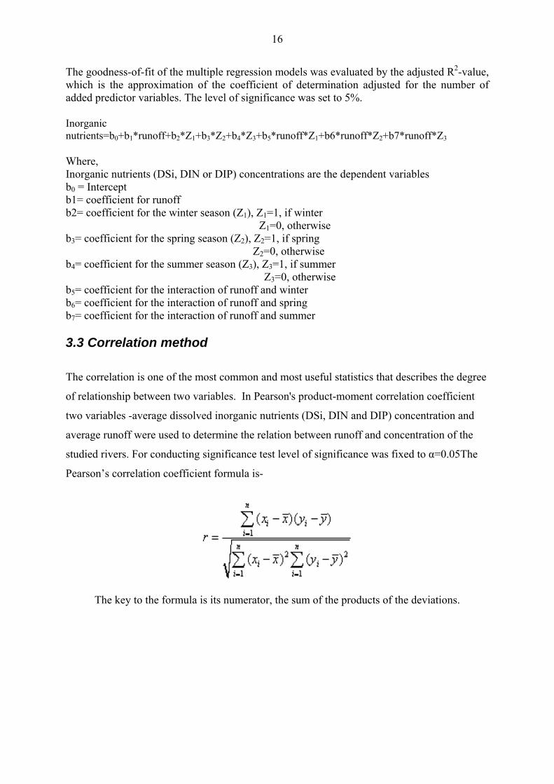
Pearson’s correlation coefficient formula is-

The key to the formula is its numerator, the sum of the products of the deviations.

17

4. General characteristics of the studied rivers and their catchments The 12 studied rivers are located all over Sweden (Figure1) .These rivers drain a great variety of catchments, ranging from almost pristine areas in northern Sweden to intensively agriculture areas in the south. In the northern Sweden river catchments population density is very sparse, <3 inhabitants/km2 (Humborg et al., 2003). The runoff in the rivers of this part is characterised by a pronounced peak during snowmelt (Bergström, 1993).Hydrological regulations, i.e. construction of river dams for power generation are the main human impact within these river systems (Humborg et al.,2001). Construction of dams for hydropower generation in northern part also resulted in high discharge in winter and low discharge in other time of the year (Bergström et al., 2001). Majorities of the northern and mid Swedish rivers are regulated to reduce peak flows, and natural lakes are present in practically all most all drainage basins (Bergström et al., 2001). Southern Sweden (46% of Sweden's total area) is the home to most of the population, agricultural lands, and industries. This part also embraces the country's large cities and metropolitan areas. The specific runoff varies a great deal from north to south as 200 mm/year in south eastern Sweden to more than 1500 mm /year in the mountains in northern Sweden (SMHI, 1994). Kalixälven Kalix River is the one of the four major and unregulated rivers in the northern Sweden, discharging in the Gulf of Bothnia near the southeast of Kalix. It is a sparsely populated basin (2 inhabitants/km2) of 23600 km2 (Humborg et al., 2003) and land covered mainly by coniferous forests (55 - 65%), peat lands (between 16 and 20%); lakes cover 4% of the area and less than 1% is farmland (Hjort, 1971). Average annual precipitation ranges from 472 - 848 mm (SMHI, 1995) and discharge 289 m3/s (SMHI, 2003). Spring snowmelt is the major event in the water discharge. Snow consists 40 -50% of the yearly precipitation in the catchment, and a large quantity of water is discharged during snowmelt at relatively low air temperatures. Most of the snow in the woodland melts in mid-May and from mountains maximum melt water discharge usually in June (Ingri et al., 2005). Piteälven Piteälven is a river in northern Sweden, flowing through the Norrbotten County. It belongs to Swedish alpine rivers, and drains into the northern part of the Gulf of Bothnia. The river is mostly unregulated with a degree of development for hydroelectric power of 4 percent. Catchment area of the river is 11 285.3 km2 (SMHI, 2003), total length is about 340 km (Melin, 1970) and lake area consists of 8.7% of the catchment (SMHI, 2002).Population density 1 inhabitant/km2 (Humborg et al., 2003). Runoff of the Piteälven mainly comes from snowmelt and summer rains but is, to a minor extent, also due to glacier melt. The annual variations in discharge are great, with a marked high-water period in July, produced primarily by snowmelt (Melin, 1970). Mean annual precipitation reaches more than 1000 mm in the western mountain ranges, but towards the east decreases to 500 mm due to rain shadow effect (Wallen, 1951). Umeälven One of the main rivers of the northern Sweden with a catchment area of 26,499 km2 , length 470 km and population density 1 inhabitant / km2 (Humborg et al., 2003). Rivers empties into the Gulf of Bothnia near the city of Umeå. Average water discharge 450 m3/s and total discharge at river mouth 14.2 km3/year (Kempe et al., 2000). It is a regulated river with an electricity generation potential of 8.4TWh. (www.umeriver.com).

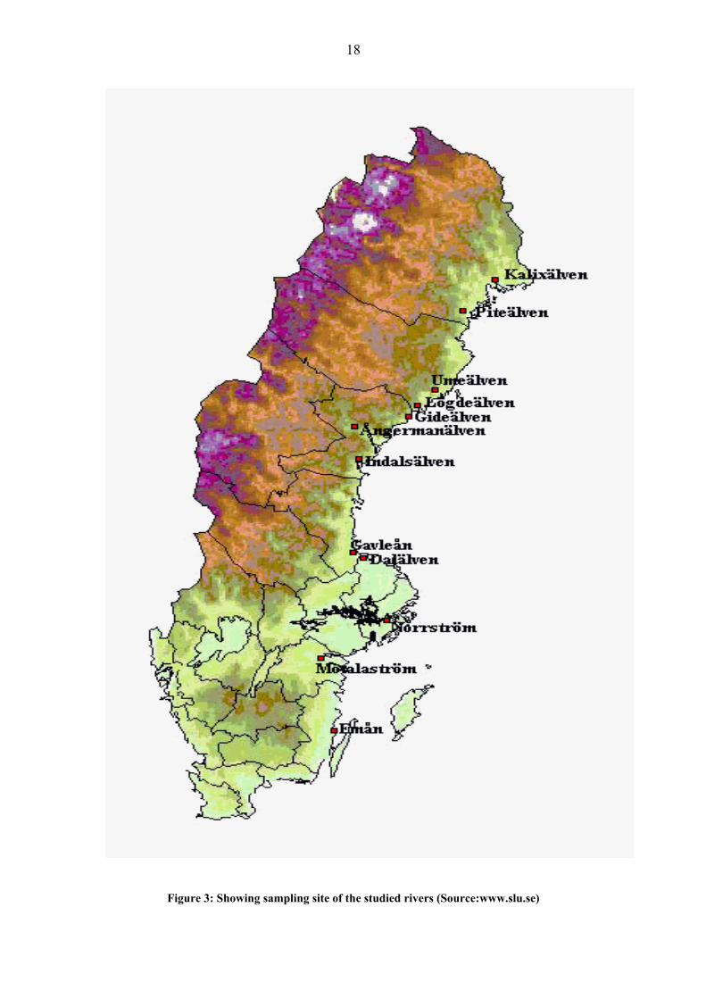
18

Figure 3: Showing sampling site of the studied rivers (Source:www.slu.se)

19

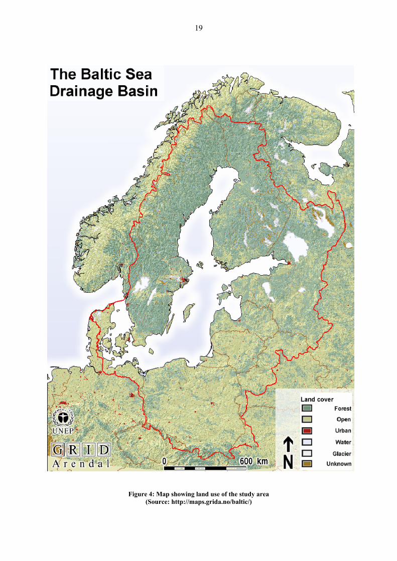
Figure 4: Map showing land use of the study area (Source: http://maps.grida.no/baltic/)

20

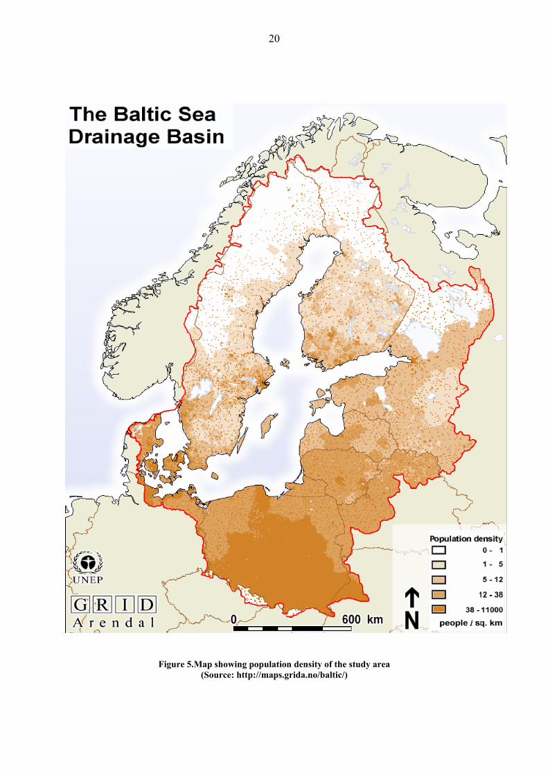
Figure 5.Map showing population density of the study area (Source: http://maps.grida.no/baltic/)

21

Lögdeälven Lögdeälven is a mountainous river; with catchment area of 1610 km2 and length 200 km. Water discharge at river mouth is 18 m3/s (NE.se). Lake area consists of 5 % of the basin (SMHI, 2002). Gideälven Gideälven is a forest dominated river of mid Norrland with catchment area of 3430 km2and length 224 km. Lake consists 5% of the total basin area (SMHI, 2002).Average water discharge is 38 m3/s (Ne.se). Ångermanälven One of the longest river with a total length 490 km and contain large volumes of water. It is a regulated river with an electricity generation potential of 7.1TWh.Total catchment area of 31,890 km2 with lake area of 9.2% and annual discharge at river mouth 490 m3/s (SMHI, 2002).Origin of this river is the mid Scandinavian mountain range, southern part of the Swedish Lappland. Ångerman river ended up in the Baltic Sea near the Kramfors town. Population density 1 inhabitant/ km2 (Humborg et al., 2003). Indalsälven Indalsälven is one of Sweden's longest rivers with a total length of 430 km. Total catchment area is 25760.7 km2 and lake area 9.9 % of the catchment (SMHI, 2002). It is a regulated river with an electricity generation potential of 8.3TWh.Main tributaries are Kallströmmen, Långan, Hårkan and Ammerån. Average water discharge at river mouth 460 m3/s (NE.se). Population density 1 inhabitants/ km2 (Humborg et al., 2003). Dalälven Dalälven is the third longest river of the Sweden with a length of 520 km and catchment area of 29 908 km2 (Humborg et al., 2003). It originates from central Sweden, flows from the north of the Dalarna and discharge into the sea in northern Upland. Average water discharge at river mouth is 379 m3/s and population density of the basin is 1 inhabitant/ km2 (Humborg et al., 2003). Northern part of this river divided into two branches: Österdalälven and Västerdalälven. It is highly regulated for hydropower generation with a capacity of 3.7 TWh and total discharge at river mouth 11.7K m3/year (Kempe et al., 2000). Gavleån: Total catchment area 2311.9 km2 and lake covers 9.5% of the basin (SMHI, 2002). River runs from large lake to Gavle bight through Gavle. Average and highest water discharge of this river is 21 m3/s and 250 m3/s respectively (NE.se). Highest water discharge usually observed during the month of April and May when snowmelt. Different industries and municipality use river water for different purposes and discharge again after use and treating at treatment plant. Norrström Norrström river basin covers an area of 22,638.8 km2 and length 300 km. Lakes area including two large lakes; Mälaren, and Hjälmaren consists 15.4% of the basin area (SMHI, 2002). Total population of this river basin is approximately 1.7million (Hannerz, 2002). Forests and mires are dominating land types which cover about 70%, agriculture areas covering approximately 20% of the area. The influence suburbs of Stockholm have spread to more than 100 km from the city and many industries have settled around the Lake Mälaren. However, some parts of the catchment is covered by heavily exploited agricultural areas, which is also a reason for supplying nutrients to the inland coastal Swedish waters (Darracq et al.,2003). Average water discharge at the river mouth is 166 m3/s (NE.se).

22

Motalaström Catchment area of Motalaström is 15,384 km2 which drains the second largest lake Vättern into the Baltic Sea at Norrköping and total lakes area is 20.6% of the basin area (SMHI, 2002). Length of the river is 100 km and average water discharge at river mouth is 100 m3/s (NE.se). The river basin is used for various purposes: large plains mainly used for intensive agriculture and for meat production. Forested regions with diversified farming and forestry and coastal regions with decreasing fishery activities and increasing tourist activities (Löwgren, 2002). Emån The Emån River is 220 km long situated in south-eastern Sweden with a catchment area of 4 440.9 km2 with a population of about100, 000(SMHI, 2002). Average annual precipitation is 450mm in the eastern part to 800 mm in the western part of the catchment and spring floods occur almost every year. The water discharge varies between a maximum of 232 m3/s to less than 7 m3/s (Eman.se). Major land uses are 81 % forest, dominated by pine and spruce, 8 % fields mainly used for production of potatoes, cereals, and fodder,4% pasture land and 6.5% lakes(SMHI,2002).

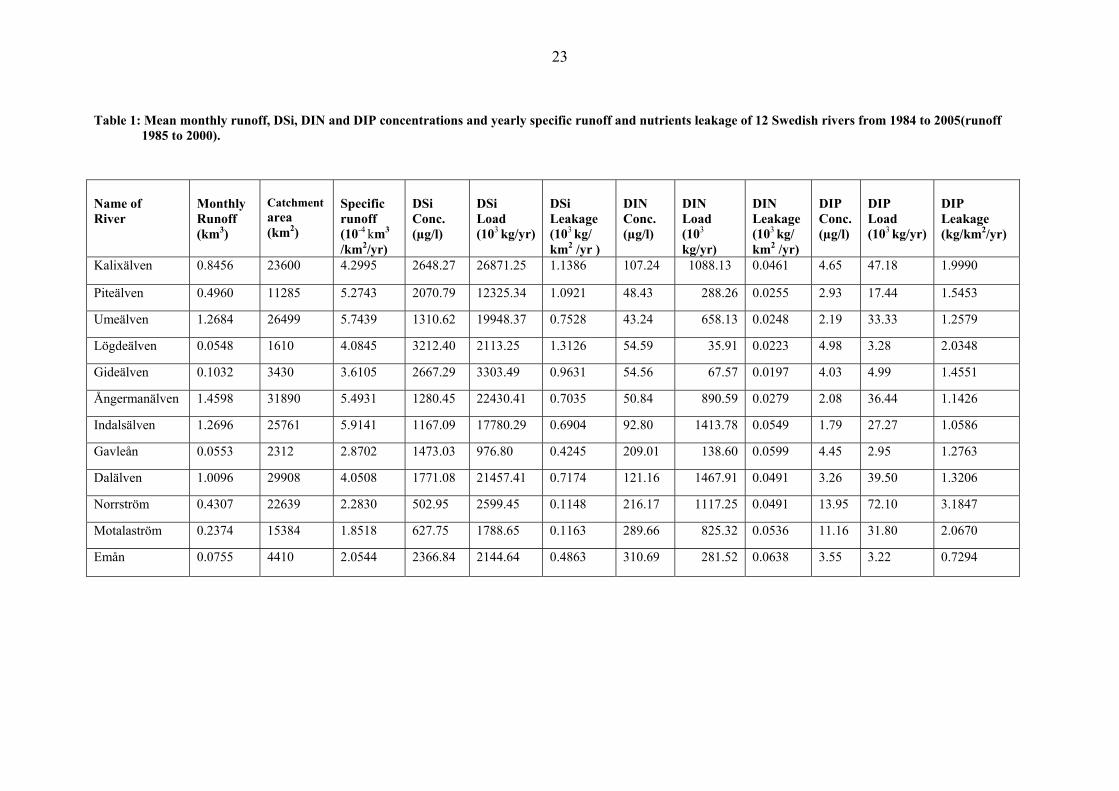
5. Results 5.1 Descriptive statistics Rivers Ångermanälven, Indalsälven and Umeälven carried higher average monthly runoff than the other river (Table1). River Lögdeälven and Gavleån, on the other hand, had very low monthly average runoff of 0.0548 km3 and 0.0553 km3 respectively. Usually rivers with low runoff demonstrated high DSi concentration e.g. Lögdeälven and Gideälven. Specific leakage of DSi found high in river Logdeälven, Kalixälven and Piteälven and low in Norrström and Motalaström. Rivers of the southern Sweden showed high DIN and DIP concentration. Among the southern river high concentrations of DIN concentration found in Emån and Motalaström. Specific leakage of DIN observed high in Emån, Gavleån and Motalaström and low in Gideälven and Lögdeälven. In case of DIP high concentration observed in Norrström and Motalaström. Specific leakage of DIP found high in Norrström, Motalaström and Lögdeälven and low in Emån and Umeälven. River Kalixälven is exceptional among the northern river where DSi, DIN and DIP concentration found high compare to other rivers in the area. High DSi concentrations observed in the rivers of the northern Sweden however, among the southern rivers Emån showed high DSi concentration. Specific runoff- observed high in Indalsälven, Umeälven and in Ångermanälven and low in Motalaström and Emån, Moderate specific runoff found in Kalixälven, Lögdeälven and Dalälven (Table1)Specific leakage of DIN and DIP among the rivers varied three degree of magnitude. In case of DIN specific leakage observed 0.0197x103 kg/km2 /year in Gideälven and in Emån it was 0.0638x103 kg/km2 /year. Specific leakage of DIP observed 0.7294 kg/km2 /year in Emån and in Norrström it was 3.1847 kg/km2 /year. In case of DSi specific leakage varied 11 degree of magnitude among the studied rivers. In Norrström leakage found 0.1148x103kg/km2 /year where as in Lögdeälven it was 1.3126x103kg/km2/year

23

Table 1: Mean monthly runoff, DSi, DIN and DIP concentrations and yearly specific runoff and nutrients leakage of 12 Swedish rivers from 1984 to 2005(runoff

1985 to 2000). Name of River

Monthly Runoff (km3)

Catchment area (km2)

Specific runoff (10-4 km3

/km2/yr)

DSi Conc. (µg/l)

DSi Load (103 kg/yr)

DSi Leakage (103 kg/ km2 /yr )

DIN Conc. (µg/l)

DIN Load (103

kg/yr)

DIN Leakage (103 kg/ km2 /yr)

DIP Conc. (µg/l)

DIP Load (103 kg/yr)

DIP Leakage (kg/km2/yr)

Kalixälven 0.8456 23600 4.2995 2648.27 26871.25 1.1386 107.24 1088.13 0.0461 4.65 47.18 1.9990

Piteälven 0.4960 11285 5.2743 2070.79 12325.34 1.0921 48.43 288.26 0.0255 2.93 17.44 1.5453

Umeälven 1.2684 26499 5.7439 1310.62 19948.37 0.7528 43.24 658.13 0.0248 2.19 33.33 1.2579

Lögdeälven 0.0548 1610 4.0845 3212.40 2113.25 1.3126 54.59 35.91 0.0223 4.98 3.28 2.0348

Gideälven 0.1032 3430 3.6105 2667.29 3303.49 0.9631 54.56 67.57 0.0197 4.03 4.99 1.4551

Ångermanälven 1.4598 31890 5.4931 1280.45 22430.41 0.7035 50.84 890.59 0.0279 2.08 36.44 1.1426

Indalsälven 1.2696 25761 5.9141 1167.09 17780.29 0.6904 92.80 1413.78 0.0549 1.79 27.27 1.0586

Gavleån 0.0553 2312 2.8702 1473.03 976.80 0.4245 209.01 138.60 0.0599 4.45 2.95 1.2763

Dalälven 1.0096 29908 4.0508 1771.08 21457.41 0.7174 121.16 1467.91 0.0491 3.26 39.50 1.3206

Norrström 0.4307 22639 2.2830 502.95 2599.45 0.1148 216.17 1117.25 0.0491 13.95 72.10 3.1847

Motalaström 0.2374 15384 1.8518 627.75 1788.65 0.1163 289.66 825.32 0.0536 11.16 31.80 2.0670

Emån 0.0755 4410 2.0544 2366.84 2144.64 0.4863 310.69 281.52 0.0638 3.55 3.22 0.7294

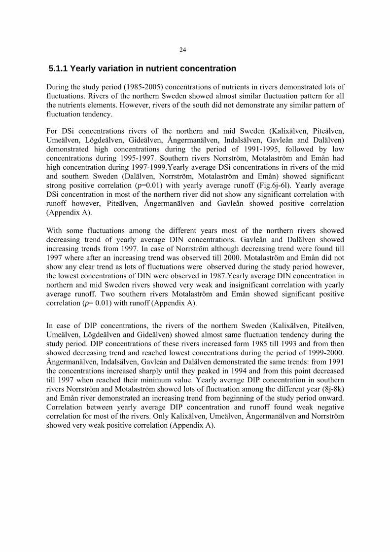
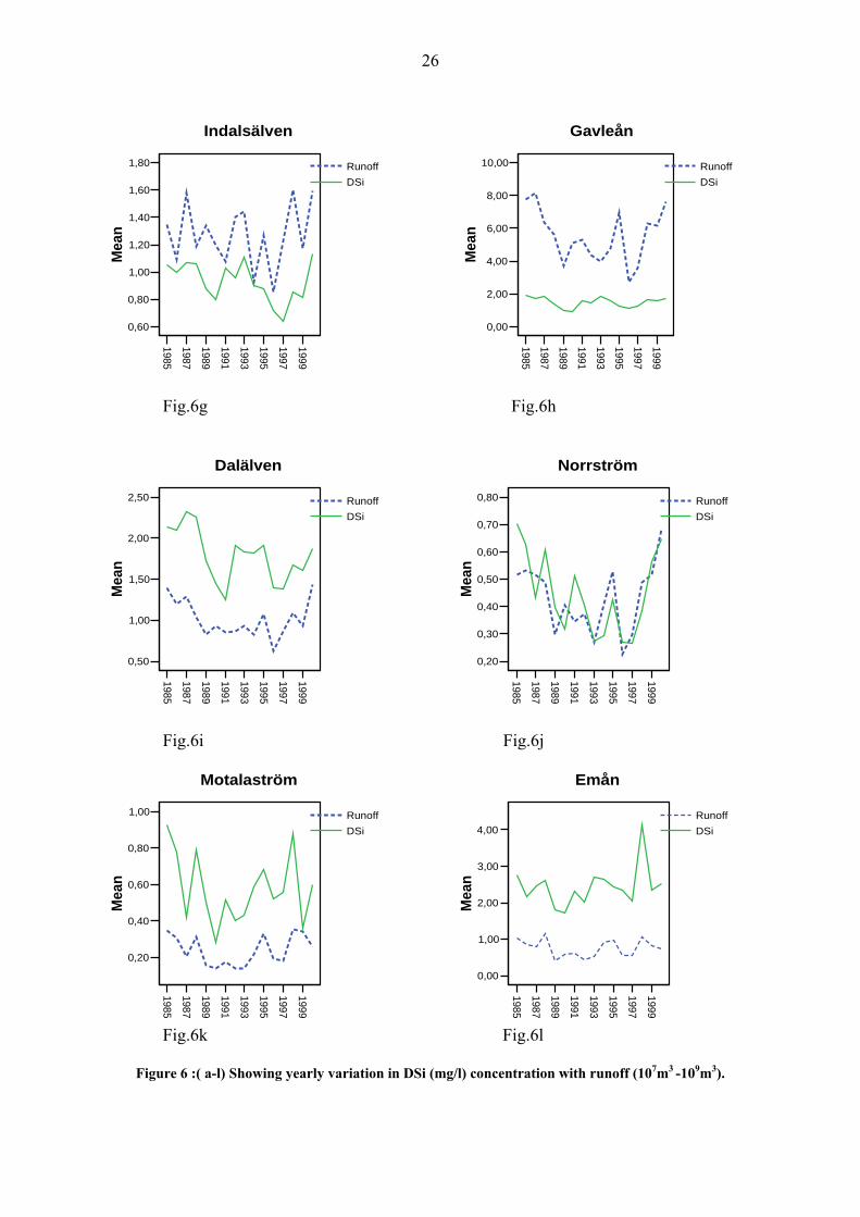
24 5.1.1 Yearly variation in nutrient concentration During the study period (1985-2005) concentrations of nutrients in rivers demonstrated lots of fluctuations. Rivers of the northern Sweden showed almost similar fluctuation pattern for all the nutrients elements. However, rivers of the south did not demonstrate any similar pattern of fluctuation tendency.

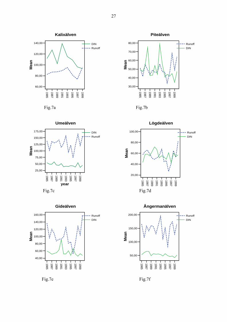
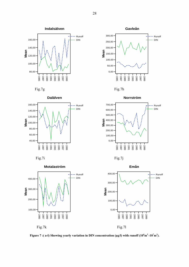
For DSi concentrations rivers of the northern and mid Sweden (Kalixälven, Piteälven, Umeälven, Lögdeälven, Gideälven, Ångermanälven, Indalsälven, Gavleån and Dalälven) demonstrated high concentrations during the period of 1991-1995, followed by low concentrations during 1995-1997. Southern rivers Norrström, Motalaström and Emån had high concentration during 1997-1999.Yearly average DSi concentrations in rivers of the mid and southern Sweden (Dalälven, Norrström, Motalaström and Emån) showed significant strong positive correlation (p=0.01) with yearly average runoff (Fig.6j-6l). Yearly average DSi concentration in most of the northern river did not show any significant correlation with runoff however, Piteälven, Ångermanälven and Gavleån showed positive correlation (Appendix A). With some fluctuations among the different years most of the northern rivers showed decreasing trend of yearly average DIN concentrations. Gavleån and Dalälven showed increasing trends from 1997. In case of Norrström although decreasing trend were found till 1997 where after an increasing trend was observed till 2000. Motalaström and Emån did not show any clear trend as lots of fluctuations were observed during the study period however, the lowest concentrations of DIN were observed in 1987.Yearly average DIN concentration in northern and mid Sweden rivers showed very weak and insignificant correlation with yearly average runoff. Two southern rivers Motalaström and Emån showed significant positive correlation (p= 0.01) with runoff (Appendix A).

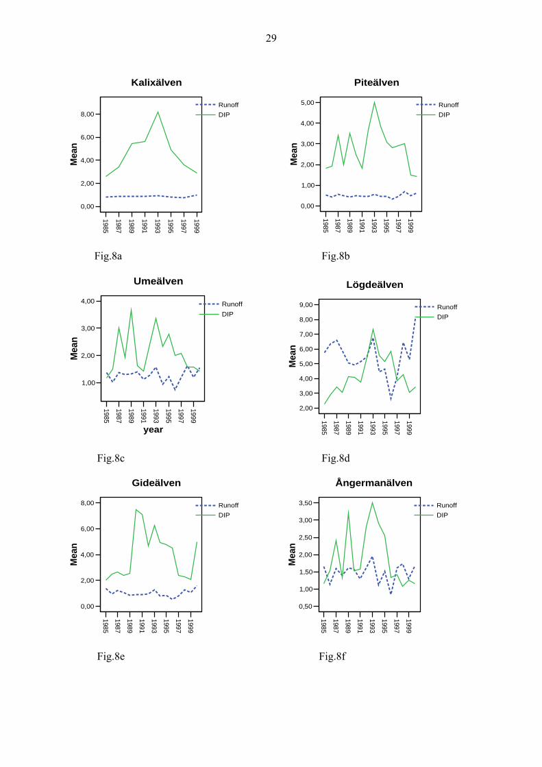
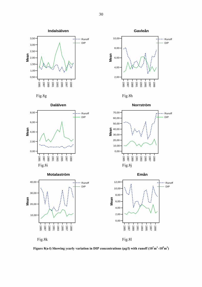
In case of DIP concentrations, the rivers of the northern Sweden (Kalixälven, Piteälven, Umeälven, Lögdeälven and Gideälven) showed almost same fluctuation tendency during the study period. DIP concentrations of these rivers increased form 1985 till 1993 and from then showed decreasing trend and reached lowest concentrations during the period of 1999-2000. Ångermanälven, Indalsälven, Gavleån and Dalälven demonstrated the same trends: from 1991 the concentrations increased sharply until they peaked in 1994 and from this point decreased till 1997 when reached their minimum value. Yearly average DIP concentration in southern rivers Norrström and Motalaström showed lots of fluctuation among the different year (8j-8k) and Emån river demonstrated an increasing trend from beginning of the study period onward. Correlation between yearly average DIP concentration and runoff found weak negative correlation for most of the rivers. Only Kalixälven, Umeälven, Ångermanälven and Norrström showed very weak positive correlation (Appendix A).

25

1985

1987

1989

1991

1993

1995

1997

1999

0,50

1,00

1,50

2,00

2,50

3,00

3,50

Mea

n

RunoffDSi

Kalixälven

1985

1987

1989

1996

1993

1995

1997

1999

0,00

1,00

2,00

3,00

4,00

5,00

Mea

n

RunoffDSi

Piteälven

Fig.6a Fig.6b

1985

1987

1989

1991

1,65

1995

1997

1999

year

0,50

0,75

1,00

1,25

1,50

1,75

2,00

Mea

n

RunoffDSi

Umeälven

1985

1987

1989

1991

1993

1995

1997

1999

2,00

4,00

6,00

8,00

10,00M

ean

RunoffDSi

Lögdeälven

Fig.6c Fig.6d

1985

1987

1989

1991

1993

1995

1997

1999

0,50

1,00

1,50

2,00

2,50

3,00

3,50

Mea

n

RunoffDSi

Gideälven

1985

1987

1989

1991

1993

1995

1997

1999

0,80

1,00

1,20

1,40

1,60

1,80

2,00

Mea

n

RunoffDSi

Ångermanälven

Fig.6e Fig.6f

26

1985

1987

1989

1991

1993

1995

1997

1999

0,60

0,80

1,00

1,20

1,40

1,60

1,80

Mea

n

RunoffDSi

Indalsälven

1985

1987

1989

1991

1993

1995

1997

1999

0,00

2,00

4,00

6,00

8,00

10,00

Mea

n

RunoffDSi

Gavleån

Fig.6g Fig.6h

1985

1987

1989

1991

1993

1995

1997

1999

0,50

1,00

1,50

2,00

2,50

Mea

n

RunoffDSi

Dalälven

1985

1987

1989

1991

1993

1995

1997

1999

0,20

0,30

0,40

0,50

0,60

0,70

0,80

Mea

n

RunoffDSi

Norrström

Fig.6i Fig.6j

1985

1987

1989

1991

1993

1995

1997

1999

0,20

0,40

0,60

0,80

1,00

Mea

n

RunoffDSi

Motalaström

1985

1987

1989

1991

1993

1995

1997

1999

0,00

1,00

2,00

3,00

4,00

Mea

n

RunoffDSi

Emån

Fig.6k Fig.6l

Figure 6 :( a-l) Showing yearly variation in DSi (mg/l) concentration with runoff (107m3 -109m3).

27

1985

1987

1989

1991

1993

1995

1997

1999

60,00

80,00

100,00

120,00

140,00

Mea

n

DINRunoff

Kalixälven

1985

1987

1989

1991

1993

1995

1997

1999

30,00

40,00

50,00

60,00

70,00

80,00

Mea

n

RunoffDIN

Piteälven

Fig.7a Fig.7b

19851987198919911993199519971999

year

25,00

50,00

75,00

100,00

125,00

150,00

175,00

Mea

n

DINRunoff

Umeälven

19851987198919911993199519971999

20,00

40,00

60,00

80,00

100,00

Mea

nRunoffDIN

Lögdeälven

Fig.7c Fig.7d

19851987198919911993199519971999

40,00

60,00

80,00

100,00

120,00

140,00

160,00

Mea

n

RunoffDIN

Gideälven

19851987198919911993199519971999

50,00

100,00

150,00

200,00

Mea

n

RunoffDIN

Ångermanälven

Fig.7e Fig.7f

28

19851987198919911993199519971999

80,00

100,00

120,00

140,00

160,00

Mea

n

RunoffDIN

Indalsälven

19851987198919911993199519971999

0,00

50,00

100,00

150,00

200,00

250,00

300,00

Mea

n

RunoffDIN

Gavleån

Fig.7g Fig.7h

19851987198919911993199519971999

40,00

60,00

80,00

100,00

120,00

140,00

160,00

Mea

n

RunoffDIN

Dalälven

19851987198919911993199519971999

0,00

100,00

200,00

300,00

400,00

500,00

600,00

700,00M

ean

RunoffDIN

Norrström

Fig.7i Fig.7j

19851987198919911993199519971999

100,00

200,00

300,00

400,00

Mea

n

RunoffDIN

Motalaström

19851987198919911993199519971999

0,00

100,00

200,00

300,00

400,00

Mea

n

RunoffDIN

Emån

Fig.7k Fig.7l

Figure 7 :( a-l) Showing yearly variation in DIN concentration (µg/l) with runoff (106m3 -107m3).

29

1985

1987

1989

1991

1993

1995

1997

1999

0,00

2,00

4,00

6,00

8,00

Mea

n

RunoffDIP

Kalixälven

1985

1987

1989

1991

1993

1995

1997

1999

0,00

1,00

2,00

3,00

4,00

5,00

Mea

n

RunoffDIP

Piteälven

Fig.8a Fig.8b

1985

1987

1989

1991

1993

1995

1997

1999

year

1,00

2,00

3,00

4,00

Mea

n

RunoffDIP

Umeälven

1985

1987

1989

1991

1993

1995

1997

1999

2,00

3,00

4,00

5,00

6,00

7,00

8,00

9,00

Mea

nRunoffDIP

Lögdeälven

Fig.8c Fig.8d

1985

1987

1989

1991

1993

1995

1997

1999

0,00

2,00

4,00

6,00

8,00

Mea

n

RunoffDIP

Gideälven

1985

1987

1989

1991

1993

1995

1997

1999

0,50

1,00

1,50

2,00

2,50

3,00

3,50

Mea

n

RunoffDIP

Ångermanälven

Fig.8e Fig.8f

30

1985

1987

1989

1991

1993

1995

1997

1999

0,50

1,00

1,50

2,00

2,50

3,00

3,50

Mea

n

RunoffDIP

Indalsälven

1985

1987

1989

1991

1993

1995

1997

1999

2,00

4,00

6,00

8,00

10,00

Mea

n

RunoffDIP

Gavleån

Fig.8g Fig.8h

1985

1987

1989

1991

1993

1995

1997

1999

0,00

2,00

4,00

6,00

8,00

Mea

n

RunoffDIP

Dalälven

1985

1987

1989

1991

1993

1995

1997

1999

0,00

10,00

20,00

30,00

40,00

50,00

60,00

70,00M

ean

RunoffDIP

Norrström

Fig.8i Fig.8j

1985

1987

1989

1991

1993

1995

1997

1999

10,00

20,00

30,00

40,00

Mea

n

RunoffDIP

Motalaström

1985

1987

1989

1991

1993

1995

1997

1999

0,00

2,00

4,00

6,00

8,00

10,00

12,00

Mea

n

RunoffDIP

Emån

Fig.8k Fig.8l

Figure 8(a-l) Showing yearly variation in DIP concentrations (µg/l) with runoff (107m3 -109m3)

31

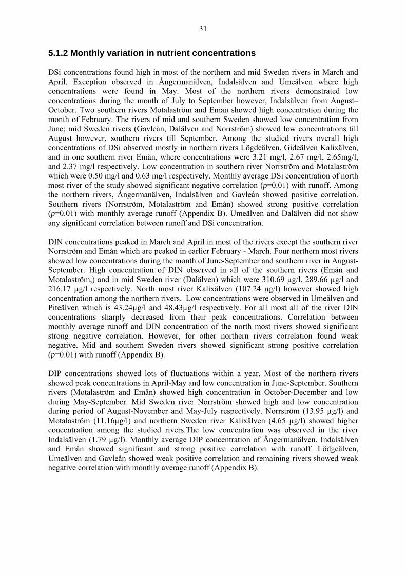
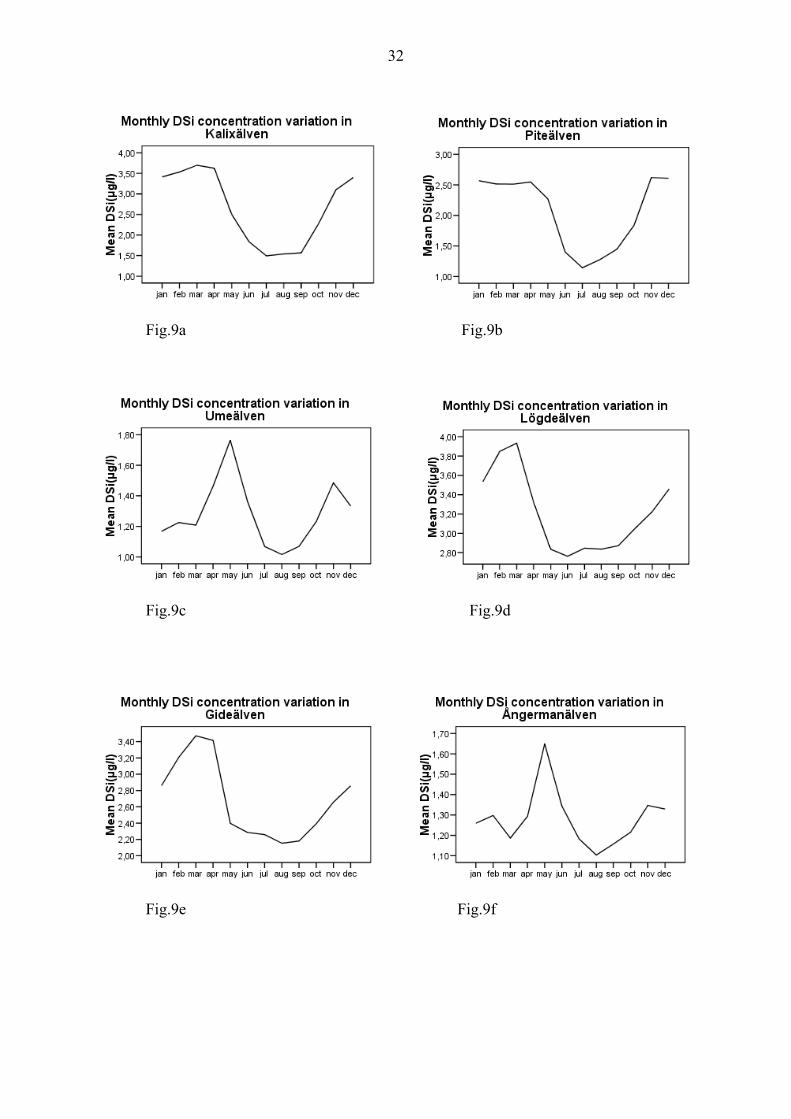
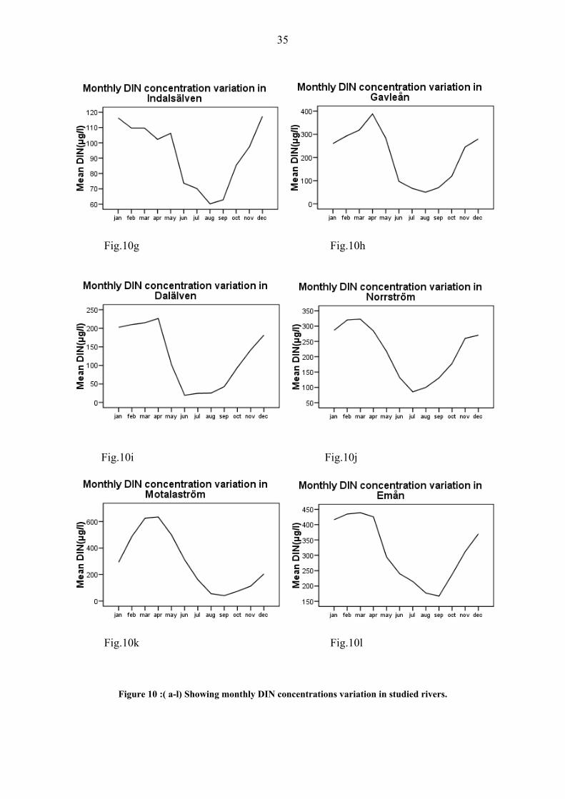
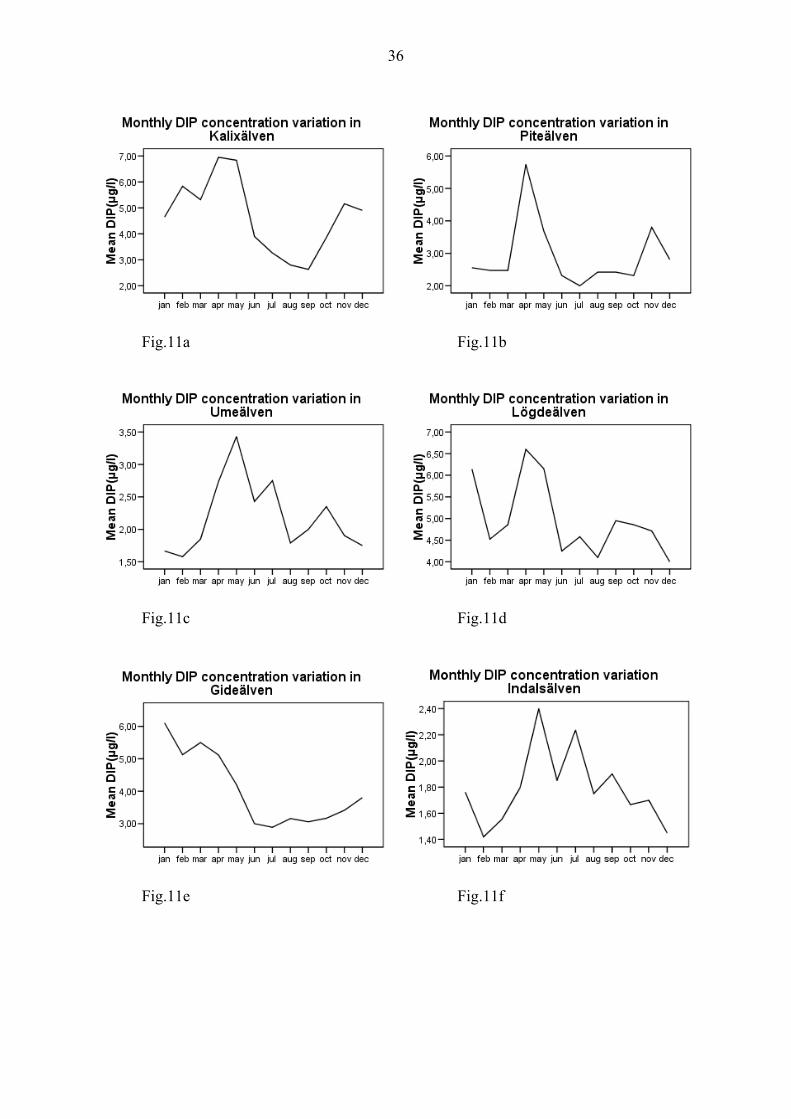
5.1.2 Monthly variation in nutrient concentrations DSi concentrations found high in most of the northern and mid Sweden rivers in March and April. Exception observed in Ångermanälven, Indalsälven and Umeälven where high concentrations were found in May. Most of the northern rivers demonstrated low concentrations during the month of July to September however, Indalsälven from August–October. Two southern rivers Motalaström and Emån showed high concentration during the month of February. The rivers of mid and southern Sweden showed low concentration from June; mid Sweden rivers (Gavleån, Dalälven and Norrström) showed low concentrations till August however, southern rivers till September. Among the studied rivers overall high concentrations of DSi observed mostly in northern rivers Lögdeälven, Gideälven Kalixälven, and in one southern river Emån, where concentrations were 3.21 mg/l, 2.67 mg/l, 2.65mg/l, and 2.37 mg/l respectively. Low concentration in southern river Norrström and Motalaström which were 0.50 mg/l and 0.63 mg/l respectively. Monthly average DSi concentration of north most river of the study showed significant negative correlation (p=0.01) with runoff. Among the northern rivers, Ångermanälven, Indalsälven and Gavleån showed positive correlation. Southern rivers (Norrström, Motalaström and Emån) showed strong positive correlation (p=0.01) with monthly average runoff (Appendix B). Umeälven and Dalälven did not show any significant correlation between runoff and DSi concentration. DIN concentrations peaked in March and April in most of the rivers except the southern river Norrström and Emån which are peaked in earlier February - March. Four northern most rivers showed low concentrations during the month of June-September and southern river in August-September. High concentration of DIN observed in all of the southern rivers (Emån and Motalaström,) and in mid Sweden river (Dalälven) which were 310.69 µg/l, 289.66 µg/l and 216.17 µg/l respectively. North most river Kalixälven (107.24 µg/l) however showed high concentration among the northern rivers. Low concentrations were observed in Umeälven and Piteälven which is 43.24µg/l and 48.43µg/l respectively. For all most all of the river DIN concentrations sharply decreased from their peak concentrations. Correlation between monthly average runoff and DIN concentration of the north most rivers showed significant strong negative correlation. However, for other northern rivers correlation found weak negative. Mid and southern Sweden rivers showed significant strong positive correlation (p=0.01) with runoff (Appendix B). DIP concentrations showed lots of fluctuations within a year. Most of the northern rivers showed peak concentrations in April-May and low concentration in June-September. Southern rivers (Motalaström and Emån) showed high concentration in October-December and low during May-September. Mid Sweden river Norrström showed high and low concentration during period of August-November and May-July respectively. Norrström (13.95 µg/l) and Motalaström (11.16µg/l) and northern Sweden river Kalixälven (4.65 µg/l) showed higher concentration among the studied rivers.The low concentration was observed in the river Indalsälven (1.79 µg/l). Monthly average DIP concentration of Ångermanälven, Indalsälven and Emån showed significant and strong positive correlation with runoff. Lödgeälven, Umeälven and Gavleån showed weak positive correlation and remaining rivers showed weak negative correlation with monthly average runoff (Appendix B).

32

Fig.9a Fig.9b

Fig.9c Fig.9d

Fig.9e Fig.9f

33

Fig.9g Fig.9h

Fig.9i Fig.9j

Fig.9k Fig.9l

Figure 9 :( a-l) Showing monthly DSi concentrations variation in studied rivers.

34

Fig.10a Fig.10b

Fig.10c Fig.10d

Fig.10e Fig.10f

35

Fig.10g Fig.10h

Fig.10i Fig.10j

Fig.10k Fig.10l

Figure 10 :( a-l) Showing monthly DIN concentrations variation in studied rivers.

36

Fig.11a Fig.11b

Fig.11c Fig.11d

Fig.11e Fig.11f

37

Fig.11g Fig.11h

Fig.11i Fig.11j

Fig.11k Fig.11l

Figure 11 :( a-l) Showing monthly DIP concentrations variation in studied rivers.

38

Fig.12a Fig.12b

Fig.12c Fig.12d

Fig.12e Fig.12f

39

Fig.12g Fig.12h

Fig.12i Fig.12j

Fig.12k Fig.12l

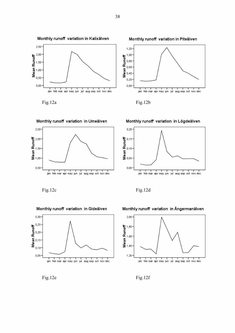
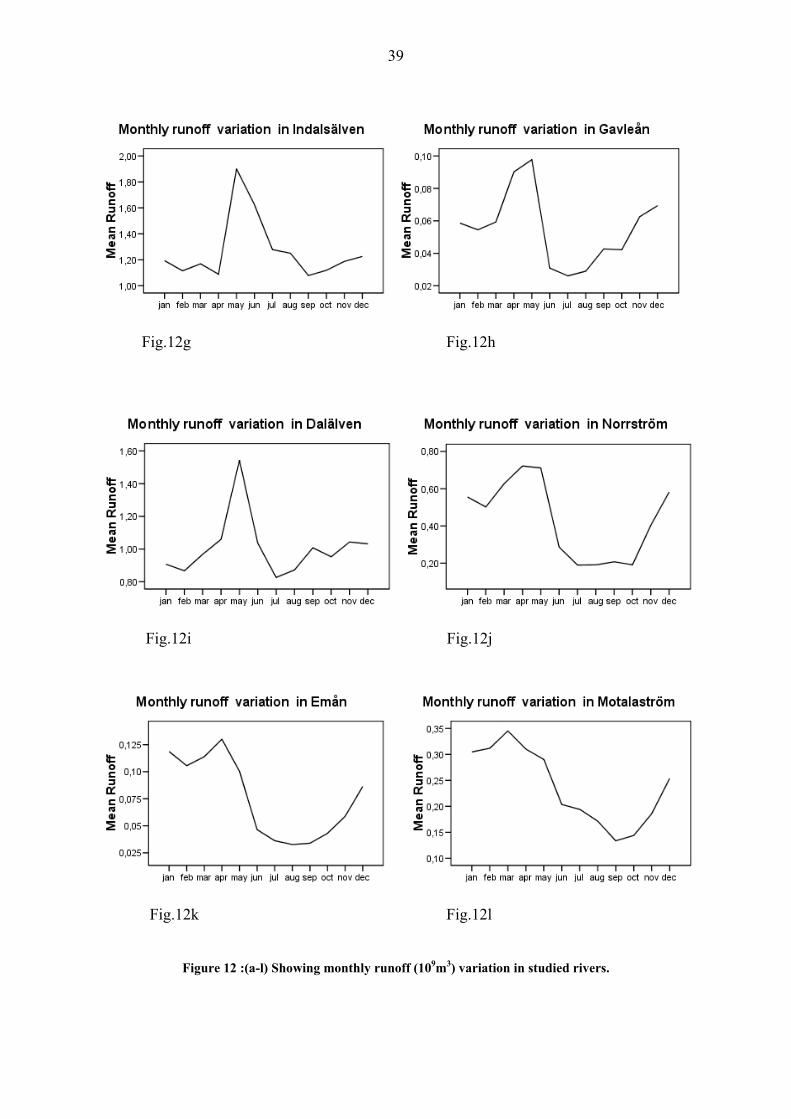
Figure 12 :(a-l) Showing monthly runoff (109m3) variation in studied rivers.

40

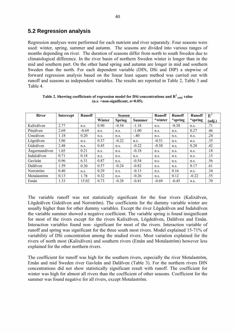
5.2 Regression analysis Regression analyses were performed for each nutrient and river separately. Four seasons were used: winter, spring, summer and autumn. The seasons are divided into various ranges of months depending on river. The duration of seasons differ from north to south Sweden due to climatological difference. In the river basin of northern Sweden winter is longer than in the mid and southern part. On the other hand spring and autumn are longer in mid and southern Sweden than the north. For each dependent variable (DIN, DSi and DIP) a stepwise of forward regression analysis based on the linear least square method was carried out with runoff and seasons as independent variables. The results are reported in Table 2, Table 3 and Table 4.

Table 2. Showing coefficients of regression model for DSi concentrations and RPP

2 PBPB(adj) BB valueBB

(n.s. =non-significant, α=0.05).

Season River Intercept Runoff Winter Spring Summer

Runoff*winter

Runoff *spring

Runoff *spring

RPP

2PP

(adj.) Kalixälven 2.77 n.s. 0.90 -0.54 -1.18 n.s. -0.58 n.s. .71 Piteälven 2.69 -0.69 n.s. n.s. -1.00 n.s. n.s. 0.27 .46 Umeälven 1.18 0.20 n.s. n.s. -.40 n.s. n.s. n.s. .24 Lögeälven 3.06 n.s. 0.37 -0.22 n.s. -0.51 n.s. n.s. .35 Gideälven 2.48 n.s. 0.45 n.s. -0.22 -0.58 n.s. 0.20 .42 Ångermanälven 1.05 0.21 n.s. n.s. -0.18 n.s. n.s. n.s. .18 Indalsälven 0.71 0.18 n.s. n.s. n.s. n.s. n.s. n.s. .15 Gavleån 0.96 6.31 0.87 n.s. -0.54 n.s. n.s. n.s. .56 Dalälven 1.59 0.30 0.57 -0.24 -0.82 n.s. n.s. 0.17 .61 Norrström 0.40 n.s. 0.29 n.s. -0.13 n.s. 0.16 n.s. .34 Motalaström 0.13 1.78 0.32 n.s. -0.26 n.s. 0.12 -0.22 .55 Emån 1.33 15.02 0.73 -0.28 -0.41 -0.69 -0.45 n.s. .70 The variable runoff was not statistically significant for the four rivers (Kalixälven, Lögdeälven Gideälven and Norrström). The coefficients for the dummy variable winter are usually higher than for other dummy variables. Except the river Lögdeälven and Indalsälven the variable summer showed a negative coefficient. The variable spring is found insignificant for most of the rivers except for the rivers Kalixälven, Lögdeälven, Dalälven and Emån. Interaction variables found non- significant for most of the rivers. Interaction variable of runoff and spring was significant for the three south most rivers. Model explained 15-71% of variability of DSi concentration among the studied rivers. Most variation explained for the rivers of north most (Kalixälven) and southern rivers (Emån and Motalaström) however less explained for the other northern rivers. The coefficient for runoff was high for the southern rivers, especially the river Motalaström, Emån and mid Sweden river Gavleån and Dalälven (Table 3). For the northern rivers DIN concentrations did not show statistically significant result with runoff. The coefficient for winter was high for almost all rivers than the coefficient of other seasons. Coefficient for the summer was found negative for all rivers, except Motalaström.

41

Table 3.Showing coefficients of regression model for DIN concentrations and RPP

2 PBPB(adj) BBvalue

(n.s. =non-significant, α=0.05).

Season Name of river Intercept Runoff Winter Spring Summer

Runoff* winter

Runoff* spring

Runoff* summer

RPP

2PP

(adj.) Kalixälven 59.50 n.s. n.s. n.s. -35.72 -176.42 n.s. n.s. .75 Piteälven 35.64 n.s. 48.46 n.s. -23.83 n.s. n.s. n.s. .37 Umeälven 35.89 n.s. 37.18 n.s. -20.17 n.s. n.s. n.s. .62 Lögdeälven 45.15 n.s. 37.02 n.s. -19.95 n.s. n.s. n.s. .52 Gideälven 55.07 n.s. 28.96 -20.11 -25.91 n.s. n.s. n.s. .49 Ångermanälven 34.09 5.95 36.82 16.86 -18.78 n.s. -12.30 n.s. .64 Indalsälven 96.75 n.s. 18.58 n.s. -29.01 n.s. n.s. n.s. .47 Gavleån 141.11 768.73 96.17 47.98 -108.31 -44.19 n.s. n.s. .49 Dalälven 95.11 15.71 90.25 n.s. -80.73 n.s. n.s. n.s. .62 Norrström 232.73 n.s. 75.27 -56.63 -83.13 n.s. 68.97 65.54 .40 Motalaström 17.27 520.43 231.61 295.92 n.s. 64.67 94.10 n.s. .73 Emån 282.91 416.40 107.25 n.s. -110.47 n.s. 37.28 n.s. .58 For the most rivers the interaction variables were not significant. Interaction variable of runoff and spring found significant for three south most rivers and interaction variable of runoff and summer found significant for only Norrström. Model explained 37-75% of DIN concentration variability. Variability explained much for the north most and southern river.

Table 4.Showing coefficients of regression model for DIP concentrations and RPP

2 PBPB(adj) BBvalue

(n.s. = non-significant, α=0.05).

season Name of river Intercept Runoff Winter Spring Summer

Run* winter

Run* spring

Run* summer

RPP

2PP

(adj.) Kalixälven 4.83 n.s. n.s. n.s. -2.10 n.s. n.s. n.s. .08 Umeälven 1.31 0.62 n.s. n.s. n.s. n.s. n.s. n.s. .06 Lögdeälven 4.07 n.s. n.s. n.s. n.s. n.s. 0.59 n.s. .04 Gideälven 3.00 n.s. 3.82 n.s. n.s. 3.67 n.s. n.s. .17 Ångermanälven 0.77 0.75 n.s. n.s. n.s. -1.09 n.s. n.s. .09 Indalsälven 1.92 n.s. -0.41 n.s. n.s. n.s. n.s. 0.25 .04 Norrström 15.63 n.s. n.s. -7.86 n.s. n.s. n.s. n.s. .08 Motalaström 18.87 n.s. -6.25 -13.71 -10.40 n.s. n.s. n.s. .40 Emån 2.27 7.13 0.64 n.s. n.s. n.s. n.s. n.s. .13 Variable runoff was significant for the river Umeälven, Ångermanälven and Emån. Variables winter explained the variability in DIP concentration in Gideälven, Indalsälven, Motalaström and Emån and spring Norrström and Motalaström. Interaction variables also found non- significant for most of the rivers. The model explained 40% of DIP concentrations variability in Motalaström, for other rivers it was less than 20%

The regression line depicts the best prediction of the dependent variable given the independent variables. But it is rarely predict perfectly. The variation observed around the fitted regression line (Appendix C). Deviation of a particular point from the regression line is residual value. There are various statistical tools used for regression model validation like statistic but different types of plot s of residuals from a fitted model provide information regarding different aspect of the model. Graphical methods have an advantage over numerical method as they can readily illustrate the complex aspects of relationship between the data and the model.

42

6 Discussion Variations of nutrients concentrations with discharge imply that the dissolved nutrients concentrations reflect hydrological and chemical processes of the catchment (Mulholland et al., 1990). Rate of water discharge may change the nutrients concentrations in different seasons by various ways like-dilution, leaching of fertilizers from terrestrial environment after precipitation, or increased land erosion. Temporal and spatial variation in nutrients concentration can be driven by both external load and internal processing (Lampman et al., 1999). Inputs from non-point sources generally increase with discharges which result in seasonal variability in nutrient transport. The concentrations of dissolved inorganic nutrients in runoff showed different patterns. Some nutrient element (DSi) decline during the periods of high discharge while others increase in concentration or remain unchanged. The specific pattern varies from catchment to catchment, amount of runoff and from period of the year. Specific leakage of nutrients elements which varied from catchment to catchment due to difference in land use, population density and other geological factors also play important role in relation between the concentrations of nutrients and runoff. 6.1 Dissolved Silica (DSi) Dissolved silica concentrations in river water depend on chemical weathering, hydrological cycle in the basin, biological process and dissolution on land and in water (Derry et al., 2001). Rate of chemical weathering controlled by complex interaction of climate, geology and biology. A recent study reported that terrestrial biogeochemical cycle significantly affected the flux of silica in river water (Conely, 2002). Temporal patterns in silica concentrations of the studied river water showed a strong seasonal dependence, similar to other studies e.g. Probst (2001). Rivers of the northern and mid Sweden showed high concentrations of DSi during the late winter and early spring season and concentration decreased through spring to summer. Regression model (Table 2) showed for most of the northern river runoff was not significant however, for the south most rivers and a mid Sweden river (Gavleån) with low average runoff was significant. High concentration in winter may be due to low temperature of water body and lack of sunlight which is not favourable for the growth of phytoplankton (Schloss et al., 2002). During winter water come to river from ground water as temperature is very low in this sub arctic environment (Humborg et al., 2006). Usually DSi concentration in ground water is higher than the surface water where percolation through soils increases weathering reactions (Drever, 1997). Silica transportation to the river through ground water is controlled by seasonal recharge and solubility, solubility usually increases with temperature (Probst, 2001). Quantity of precipitation received by drainage basin due to seasonal variation and residence time of ground water also influence silica concentration. After winter the concentrations tend to decrease in spring as during this season temperature, sunlight, other required nutrients and all other factors required for diatom growth are favourable. Kennedy (1971) explained that, in most cases, dilution and biological uptake by diatoms are the cause of low concentration of dissolved silica in river water. Adsorption of silica on suspended particles could also possibly remove silica from solution in the presence of electrolytes (Bien et al., 1958). Increased runoff, due to higher precipitation recharge of

43

ground water system gets less time to interact with rocks and sediment also resulting lower concentration in ground and river water (Probst, 2001). There are low concentrations in summer as DSi is used up by the phytoplankton during their growing period in spring. The process of production, transport and dilution of silica within a catchment can be used to explain the causes of variation in silica concentrations in rivers due to the seasonal difference in runoff regime (Sigelo et al., 2002). Silica dissolution from quartz and silicate minerals varies reasonably, and as this process is very slow, part of the reason for the low concentrations in natural waters is the slowness of the dissolution process. During the autumn, there was apparent increase in silica concentrations that may be due to a surplus of dissolved silica relative to other nutrients (Sigelo et al., 2002) or decomposed inorganic silica back to the upper layer due to vertical movement caused by cooling of surface layer(Harashima, 2005). In the southern and mid Sweden yearly average temperature is high, the river runoff is low and there is more arable land compare to the northern part. Higher average temperature and arable land by increasing tillage may enhance the weathering rate of silica (Conely et al., 2000) this may cause a positive correlation with runoff. Some northern river with low runoff and less regulation were found positively correlated with runoff, where low runoff did not cause any dilution affect and less regulation caused lower rate of retention. Characteristics of bed rock geology of the catchment is also an important factor for the DSi concentration of the river, usually high concentrations observed in a basin with basic volcanic bed rock (Humborg et al, 2006). Difference in soil type and presence of H+ ion in soil may also increase the DSi concentrations by influencing weathering rate (Land et al., 1998). In northern Sweden rivers runoff is high and mostly regulated; high runoff and retention cause dilution of silica upstream of the dams. Semhi et al., (2000) observed a weak correlation between DSi concentration and water discharge from the Garonne river basin, France. In this study rivers of the southern Sweden, like Norrström and Motalaström showed low DSi concentrations although the runoff was moderate in quantity. Low concentrations in these rivers can be explained as basin of Norrström river drains large city which bring large quantities of phosphate. As fresh water body are P limited high P concentration in water course lead high deposition of DSi by diatom production. Runoff from both the rivers comes through lakes. Rivers with lakes outflow were found to have low DSi concentrations in previous study of Sweden and other part of the world (Schelske, 1985; Conely et al., 2000) where in-lake processes influence diatom growth and subsequent burial of diatom in the sediment with long residence time (Hecky et al., 1988). On the other hand high DSi concentration found in the free flowing northern rivers (Lögdeälven, Gideälven and Kalixälven) and one agricultural dominated Emån river. It has been observed that DSi weathering is much lower in the regulated boreal river system (Humborg et al., 2002). Hydrological alteration due to dams decrease weathering rate of silica by inundation of vegetation, loss of soil and underground channelling which prevent interaction of surface water with vegetated soil and ground water (Humborg et al., 2006). Comparison of discharge weighted annual DSi concentration of unperturbed Kalixälven and dammed Luleälven showed concentration in former observed twice as the latter and yield was only 40% in the dammed river than the free flowing Kalixälven (Humborg et al., 2006). Among the rivers runoff of Lögdeälven and Emån was very low compare to other studied rivers. Local geology, weathering rate of these basin or other co variable may be the cause of

44

this higher concentration with low runoff. Conely et al., (2000) found a weak but significant correlation (r2=.18, p<0.05) between the percentage of cropland in the catchment and concentrations of DSi which can explain high concentration in agriculture dominated Emån river. Terrestrial vegetation forming phytoliths add significant amount of Biogenic silica (BSi) to the soil (Conely, 2002) and solubility of amorphous silica is five times faster than the mineral silicate (Hurd, 1983). Changes in agricultural practice and soil erosion increase mobilization of amorphous soil silica to aquatic environment (Hartmann & Kempe, 2005; Humborg et al., 2006). Monthly average DSi concentration in north most rivers showed negative correlation with runoff due to high runoff from basin during the months of increased precipitation. Although specific leakage of DSi in this part of the river found high compare to other river however higher specific runoff may be the possible cause of negative correlation with runoff. Some northern rivers with low runoff showed positive correlations which may be due to low runoff prevent dilution affect. River of the southern river showed positive relation as specific runoff is low compare to northern rivers. Type of soil present in the basin also an important factor that influence the weathering rate of DSi, like presence of pyretic soil, which by releasing sulphuric acid enhances the weathering rate of DSi as can be observed in a tributary to Lake Hjälmaren where high concentrations DSi have been reported due to presence of acid pyretic soils (Conely et al., 2000). 6.2 Dissolved Inorganic Nitrogen (DIN) DIN concentrations varied markedly among the studied rivers and showed a high variability over time. Concentrations increased from north to south and patterns varied depending on seasons and runoff conditions. The spatial and temporal variations in the studied river water DIN concentrations can be attributed to various catchment characteristics like soil type, topography, land use, point source and hydrological regime which control the transport and storage of DIN (Lepistö, 1995). In general, losses of nitrogen correspond with variation in runoff (Stålnacke etal., 1999) as nitrate is highly soluble relative to other nutrients. As a result, the concentration of nitrate simply increases as water flow increases (Hill et al., 1999). No such correlation was found for the rivers considered. Positive relationship between monthly average DIN concentration and runoff was observed for the river of mid and southern Sweden. The positive correlation of DIN concentrations with water discharge during the season of peak water flow can be considered that the NO3 supply accumulated near the soil surface was quickly depleted in response to the runoff. This characteristic behaviour, termed the ‘flushing effect’, has been observed by Murdoch and Stoddard (1992). Arheimer (1998) explained the flushing effect by the fact that usually nutrients are more available in the lower parts of a catchment from where water can easily access to the river and consequently has a quick response to river flow generation. Specific leakage of the southern river observed high and specific runoff was low which prevent dilution. Opposite relation observed for the northern rivers where high specific runoff and low specific leakage may be the plausible cause of negative correlation between runoff and DIN concentration. Relationship between NO3 concentration -runoff and NO3 flux-runoff were examined for one European river Zwalm catchment, Belgium and found a positive correlation between NO3 concentration and runoff (Herpe & Troch, 2000). Some rivers of this study exerted different average monthly concentration pattern with runoff (Table 1). Like in Umeälven and

45

Ångermanälven where average monthly runoff was high compared to other studied rivers but DIN concentration observed low which contradicts with the concentration-runoff relation found in Zwalm river. Land use practice may be the cause of such relationship. In case of Emån and Gavleån, where average monthly runoff was markedly low, but DIN concentration found high compare to other studied rivers. Low DIN concentrations with high runoff or high concentrations with low runoff can be explained by the land use pattern of that catchment. Substantial variation in N losses may occur in two catchment with same runoff quantity due to the fact of having different types of soil and cropping pattern (Vagstad et al., 2004). Usually the catchment where agricultural activities are intensive and manage forestry are practiced even low runoff would lead to high amount of dissolve nitrate to receiving water bodies. On the other hand, the catchment where agricultural and forest activities are not intensive or even absent, higher runoff would not be able to contribute to concentration increase; instead concentrations may decrease due to dilution effect. Negative correlation between runoff and DIN concentration observed in northern rivers where agricultural activities are less or absent along with high average runoff may cause dilution. In this part precipitation through rain or snowmelt, bringing water from the upper parts of the catchment which is mostly mountainous. Water with low NO3 concentrations from the upper parts of the catchment will dilute the river NO3 concentration (Probst, 1985). River retention and removal also reduce the role of upstream sources (Tonderski et al., 1997), which may be the cause of weak and insignificant correlation with runoff. Regarding seasonal variation of DIN concentrations northern rivers peaked in March and April. However, southern river Norrström and Emån earlier in February. Delay in northern Sweden rivers may be due to climatological factors as average temperature of north is much lower than mid and south Sweden and temperature remains low for a longer period which delays snowmelt. Regression model (Table 3) predicted high concentration in winter, a decrease in spring and reached lowest concentration in summer. For the northern river runoff was not significant. However, for agriculture dominated Emån, Motalaström and Gavleån runoff played significant role in DIN concentration. For the river Norrström runoff was not significant as from this river basin DIN mostly coming from point sources. Nitrate loading is usually found high in late winter and early spring due to soil-water recharge in autumn and winter, and N mineralization increases when soil drying is following by re-wetting (Tranter et al., 1992). The highest surface water NO3 concentrations and loadings from snow-covered forested watersheds occur during moderate to high flow caused by snowmelt in winter and spring as solutes stored in snow packs are released during melting (Tranter et al., 1992).Nitrification in unfrozen soils also can contribute significant amounts of NO3 (Peters & Leavesley, 1995). In spring when all other physico-chemical conditions are favourable for growth a large amount of nitrate utilized when biological uptake is greatest which ultimately lower DIN concentrations. Low concentrations during the summer due to biological uptake in spring and lack of leaching being the most apparent reasons for low concentrations (Tonderski et al., 1997). Long term pattern in DIN concentration of the northern river showed considerable decline over the last several years. Rivers of this part drains forested area and there are almost no intensive agricultural activities. In forested basins, plants are taking more nutrients during their early to mid-stages of growth that result in subsequent decreases in nutrient leaching from soil (Heathwaite et al., 1996). The high values of DIN concentrations observed in the

46

river of southern and mid Sweden as a result of intensive agricultural activities in this part of the country. Strong relation between agricultural land and nitrate concentration observed in previous study of Sweden and Finland (Pitkänen, 1986) and in other country (Jordan et al, 1997). Among the southern rivers basin of Motalaström and Emån are agriculture dominated which discharge high nitrate to these rivers. A study of total N concentration and river flow in Motalaström during the period of 1969-84 showed that total N concentration increased with increased water flow (Karlsson et al., 1988). 6.3 Dissolved Inorganic Phosphate (DIP) In the arable land of Sweden during the period of 1953-1995 a surplus of 400 to 1800 kg P/hectare was added which accumulated in the soil profile (Andersson et al., 1998) with highest surplus found agriculture and animal production dominant areas. However, due to various preventive measures the surplus phosphorous has now decreased on average 3 kg P/hectare/ year (Official Statistics Sweden, 2002). DIP concentrations increased till 1994 for most of the studied rivers and then decreased which may be due to decrease in fertilizers use caused by various abatement activities taken by government (Swedish Agricultural Board, 2006). Agricultural dominated Emån river was an exception where DIP concentration increased all over the study period. In agricultural runoff phosphorous exists as some soluble inorganic phosphate combined with organic and inorganic colloidal particles. Soluble inorganic phosphorous come from applied fertilizers or from mineralization of organic compound (Heathwaite, 1996). Phosphorous transport by river is controlled by the process of sedimentation and resuspension rather than runoff quantity or temperature making the phosphorous source apportionment much more uncertain (Tonderski et al., 1997). Phosphate also comes from natural background source and it is vary from basin to basin depending on quantity of forest land, agricultural land, swamp area and basin geomorphology (Sileika et al., 2001) Monthly average DIP concentration of Ångermanälven, Indalsälven and Emån was significant and positively correlated with runoff, as also observed in other river like in Loire river, France (Köhler, 2006). Phosphate usually correlates positively with runoff as soil-P increases the particulate and dissolved forms of P along with runoff (Pote et al., 1996). P behaves differently than N and DSi. As observed in rivers with moderate and low specific leakage with high to low specific runoff showed positive relation between DIP concentration and runoff. Internal load from the river may also be the cause of such positive relation. Ulén et al. (2004) found high total P concentrations in the surface water of a catchment characterized by clay soil. Phosphorus transported from agricultural land through flash losses of soluble phosphorus soon after application of fertilizer or manure, slow-leak losses of soluble phosphorus, or erosion events (Wiederholt & Johnson, 2005). Artificial fertilizers and manure have a higher concentration of soluble phosphorous than soil. Precipitation after application of fertilizers brings high concentrations of phosphorous to the aquatic system.

Soil characteristics like Fe, pH and oxygen content of soil also play important role in DIP concentration (Smith et al., 2003) which may cause of weak relation of DIP concentration with runoff in other rivers. Sileika et al., (2002) studied Nevezis river of Lithuania and Lampman et al., (1999) Hudson river. Neither of them found any correlation between runoff, total P concentration and weather temperature. Phosphate runoff depends on factors like natural background pollution, agricultural activity, industrial and household effluents contribution etc. (USGS, 2001). Settling down of phosphate particles on the river bed or utilization by algae also decline phosphate

47

concentrations. Unlike other nutrients phosphorus is particle reactive (Howarth et al., 1995), so contribution of run-off from agricultural sources in increasing DIP concentration less important because some of the phosphorus is retained within the soil due to affinity to particle (Hessen, 1999). Presence of wetlands or buffer strips also significantly influence the transfer of particulate phosphorus to the surface water (Vought et al., 1995).

Among the studied rivers high concentrations are observed in southern river Norrström and Motalaström. Southern part is comparatively densely populated, intensive cultivation and urban waste disposal and industrial activities have enhanced the transport of phosphate from terrestrial to aquatic environments. As a consequence of these activities, supply of phosphate as well as concentrations of phosphorous in rivers has increased (Smith et al., 1987). Norrström river showed high concentration during the period of low runoff as large quantities of phosphate coming from point sources of the Stockholm and its suburban areas. Among the northern rivers Kalixälven showed high concentration as this river is free flowing where the absence of dams did not cause loss of phosphate by retention process. Dissolved inorganic phosphorus was regressed against runoff, and four seasons (Table 4). But model can not explained well for any of the rivers as we got very low adjusted R2 .Variable like natural background pollution, agricultural, urban and industrial activity, soil characteristics and basin geomorphology may play important role in river DIP concentration. P differs from other nutrients element as it is almost entirely associated with soil particles so not readily found as dissolved form. Particle size of soil is also an important factor in the phosphate transportation as fine particles can hold more P and soil erosion transport finer particles than the coarse particles causing sediment enriched with phosphorous. 6.4 Differences and similarities Concentration of nutrients elements demonstrated both similar and varying behaviour from river to river and from season to season depending on hydrological regime, land use and geology of the catchment. The river which showed highest concentration did not contain the highest runoff. High DSi concentration observed in the unperturbed northern rivers however, high DIN concentration observed in agriculture dominated river followed by river basin dominated by industrial and urban activities. River basin dominated by urban and industrial activities showed high DIP concentration than the basin dominated by other activities. Among the nutrients element DSi concentration demonstrated concentration gradients from north to south. North unperturbed rivers showed high concentration than the agriculture, urban and industrial dominated southern rivers. In case of DIN concentrations gradients seen opposite to the DSi concentration. DIP concentration did not show any north to south gradients In case of seasonal variation DSi and DIN concentration observed high in winter and decreased through spring to summer. Unfavourable condition for biological uptake by plankton and water with high DSi concentration discharged from ground water is the plausible cause of high concentration during winter. High DIN concentration in winter as soil water recharge in autumn and early winter and increased mineralization due to soil drying followed by re-wetting. Melting of snow release large amount of NO3 stored in snow pack also contributed high DIN concentration. High concentration of DIP varied from river to river, some rivers peaked during early spring and other during autumn. River which drains urban and industrial areas peaked in late summer and early autumn when runoff is low, which means

48

nutrients discharging from point sources. Behaviour of DIP varies with other nutrient elements as DIP is particle reactive and contribution from ground water is negligible. DSi and DIN concentrations in most southern river significantly and positively related with runoff. For northern rivers this relationship was negative. In case of DIP concentration except three rivers most of the rivers showed negative and insignificant relation with runoff. 7. Conclusion Among the studied rivers high concentration of DSi observed in the unperturbed rivers of northern Sweden and in agriculture dominated southern river Emån. High DIN concentration observed in agriculture dominated southern river followed by river basin dominated by industrial and urban activities. River basin of the mid and south Sweden dominated by urban and industrial activities showed high DIP. Kalixälven was exceptional where DIN and DIP concentration found higher among the northern rivers. Monthly average DSi and DIN concentration in north most river showed negative correlation with runoff as agricultural activities are absent or very low and high runoff from mountainous basin during the months of increased precipitation cause dilution. Some northern rivers with low runoff showed positive correlations with DSi where specific leakage was high but low runoff prevent dilution affect and same positive relation also observed for southern rivers. Type of soil, land use and weathering rate of the basin also an important factor influence DSi and DIN concentration. Phosphorus behaves differently from other nutrients as it is particle reactive and mostly come from point sources, DIP positively correlated with runoff for very few rivers. DSi and DIN concentration showed almost same seasonal variation. High during winter when uptake by organisms is less due to unfavorable condition for growth. Concentrations tend to decrease during growing season spring and reached low in summer. Seasonal variation in DIP differed from river to river, high concentrations ranging from early spring to early autumn. But in most rivers low concentration observed during summer. DSi, DIN and DIP were regressed against runoff and four seasons. Model explained 15-71% and 37-75% of concentration variability of DSi and DIN respectively. But model can not explained well for DIP concentration in rivers as we got very low R2(ad.) Variable like natural background pollution, agricultural, urban and industrial activity, soil characteristics and basin geomorphology may play important role in river DIP concentration.

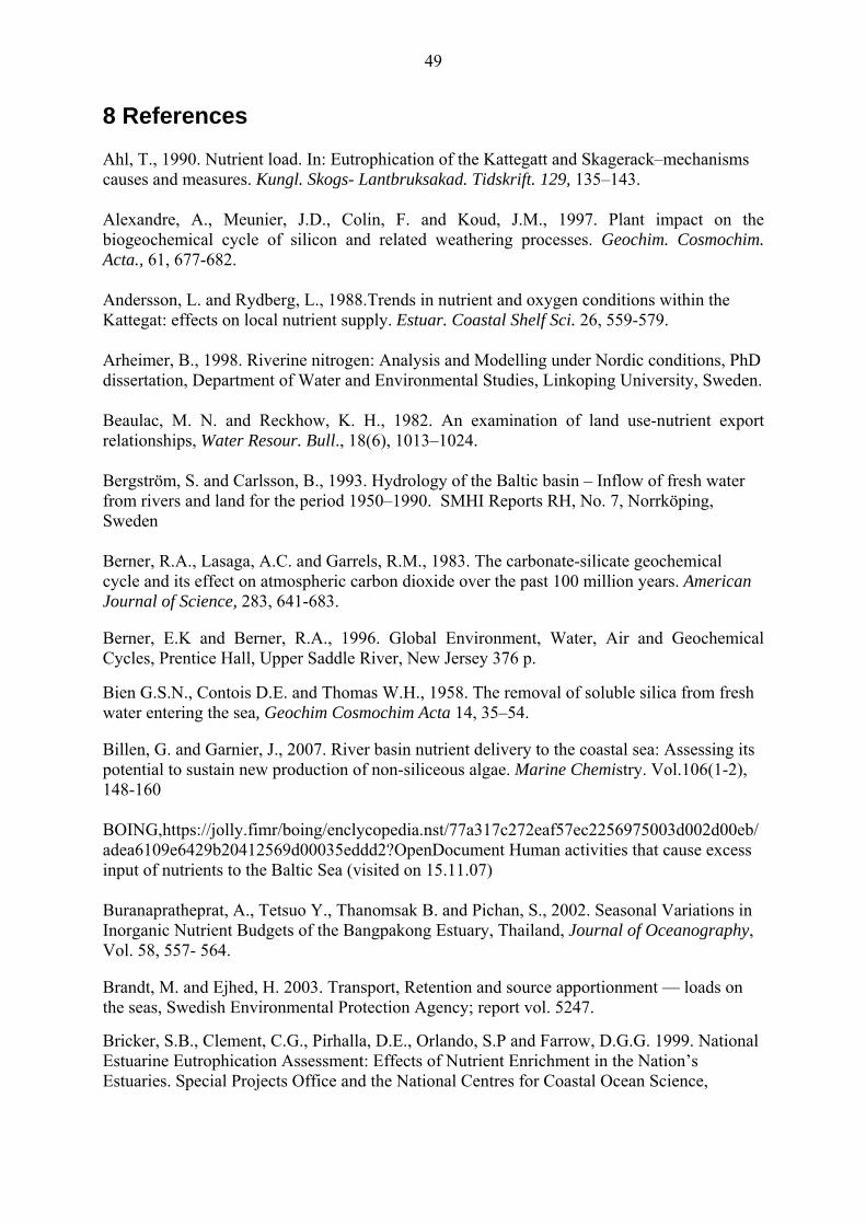
49

8 References Ahl, T., 1990. Nutrient load. In: Eutrophication of the Kattegatt and Skagerack–mechanisms causes and measures. Kungl. Skogs- Lantbruksakad. Tidskrift. 129, 135–143. Alexandre, A., Meunier, J.D., Colin, F. and Koud, J.M., 1997. Plant impact on the biogeochemical cycle of silicon and related weathering processes. Geochim. Cosmochim. Acta., 61, 677-682. Andersson, L. and Rydberg, L., 1988.Trends in nutrient and oxygen conditions within the Kattegat: effects on local nutrient supply. Estuar. Coastal Shelf Sci. 26, 559-579. Arheimer, B., 1998. Riverine nitrogen: Analysis and Modelling under Nordic conditions, PhD dissertation, Department of Water and Environmental Studies, Linkoping University, Sweden. Beaulac, M. N. and Reckhow, K. H., 1982. An examination of land use-nutrient export relationships, Water Resour. Bull., 18(6), 1013–1024. Bergström, S. and Carlsson, B., 1993. Hydrology of the Baltic basin – Inflow of fresh water from rivers and land for the period 1950–1990. SMHI Reports RH, No. 7, Norrköping, Sweden Berner, R.A., Lasaga, A.C. and Garrels, R.M., 1983. The carbonate-silicate geochemical cycle and its effect on atmospheric carbon dioxide over the past 100 million years. American Journal of Science, 283, 641-683. Berner, E.K and Berner, R.A., 1996. Global Environment, Water, Air and Geochemical Cycles, Prentice Hall, Upper Saddle River, New Jersey 376 p. Bien G.S.N., Contois D.E. and Thomas W.H., 1958. The removal of soluble silica from fresh water entering the sea, Geochim Cosmochim Acta 14, 35–54. Billen, G. and Garnier, J., 2007. River basin nutrient delivery to the coastal sea: Assessing its potential to sustain new production of non-siliceous algae. Marine Chemistry. Vol.106(1-2), 148-160 BOING,https://jolly.fimr/boing/enclycopedia.nst/77a317c272eaf57ec2256975003d002d00eb/adea6109e6429b20412569d00035eddd2?OpenDocument Human activities that cause excess input of nutrients to the Baltic Sea (visited on 15.11.07) Buranapratheprat, A., Tetsuo Y., Thanomsak B. and Pichan, S., 2002. Seasonal Variations in Inorganic Nutrient Budgets of the Bangpakong Estuary, Thailand, Journal of Oceanography, Vol. 58, 557- 564. Brandt, M. and Ejhed, H. 2003. Transport, Retention and source apportionment — loads on the seas, Swedish Environmental Protection Agency; report vol. 5247. Bricker, S.B., Clement, C.G., Pirhalla, D.E., Orlando, S.P and Farrow, D.G.G. 1999. National Estuarine Eutrophication Assessment: Effects of Nutrient Enrichment in the Nation’s Estuaries. Special Projects Office and the National Centres for Coastal Ocean Science,

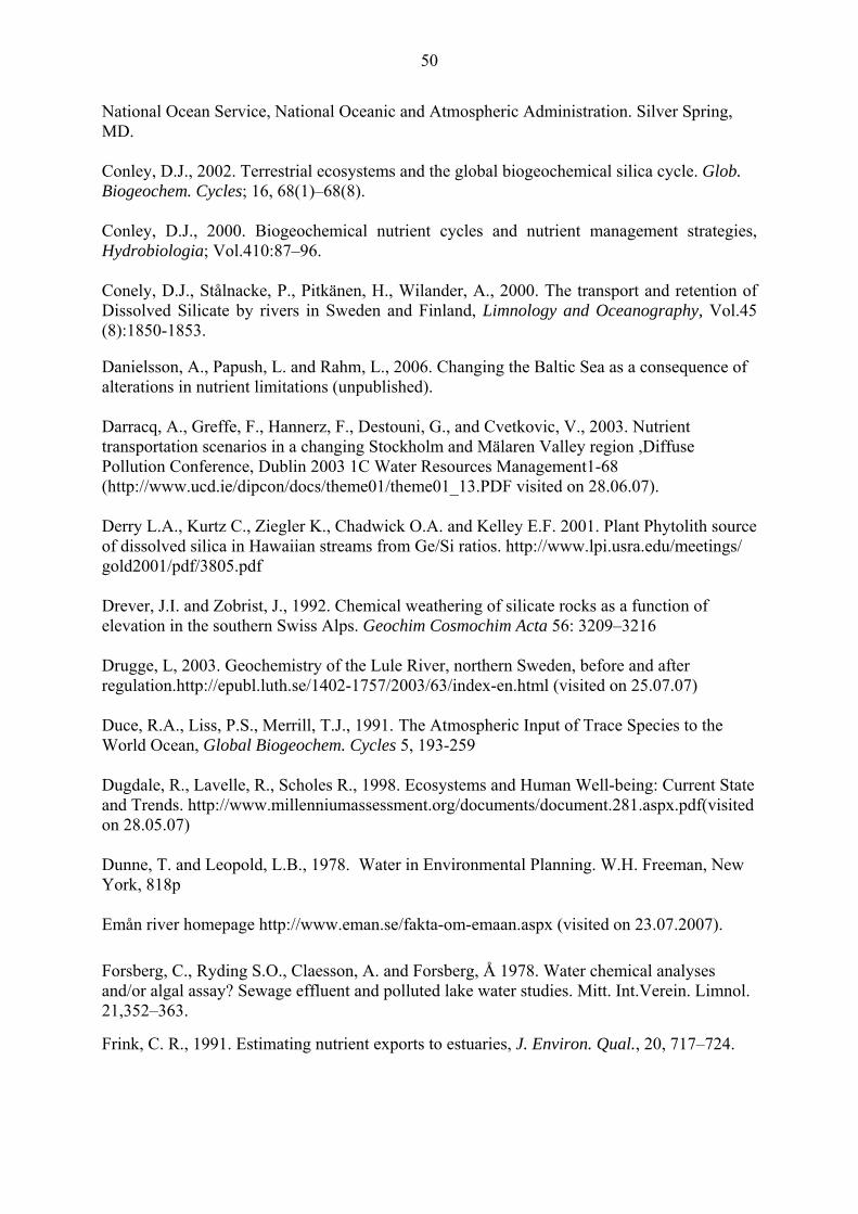
50

National Ocean Service, National Oceanic and Atmospheric Administration. Silver Spring, MD. Conley, D.J., 2002. Terrestrial ecosystems and the global biogeochemical silica cycle. Glob. Biogeochem. Cycles; 16, 68(1)–68(8). Conley, D.J., 2000. Biogeochemical nutrient cycles and nutrient management strategies, Hydrobiologia; Vol.410:87–96. Conely, D.J., Stålnacke, P., Pitkänen, H., Wilander, A., 2000. The transport and retention of Dissolved Silicate by rivers in Sweden and Finland, Limnology and Oceanography, Vol.45 (8):1850-1853. Danielsson, A., Papush, L. and Rahm, L., 2006. Changing the Baltic Sea as a consequence of alterations in nutrient limitations (unpublished). Darracq, A., Greffe, F., Hannerz, F., Destouni, G., and Cvetkovic, V., 2003. Nutrient transportation scenarios in a changing Stockholm and Mälaren Valley region ,Diffuse Pollution Conference, Dublin 2003 1C Water Resources Management1-68 (http://www.ucd.ie/dipcon/docs/theme01/theme01_13.PDF visited on 28.06.07). Derry L.A., Kurtz C., Ziegler K., Chadwick O.A. and Kelley E.F. 2001. Plant Phytolith source of dissolved silica in Hawaiian streams from Ge/Si ratios. http://www.lpi.usra.edu/meetings/ gold2001/pdf/3805.pdf Drever, J.I. and Zobrist, J., 1992. Chemical weathering of silicate rocks as a function of elevation in the southern Swiss Alps. Geochim Cosmochim Acta 56: 3209–3216 Drugge, L, 2003. Geochemistry of the Lule River, northern Sweden, before and after regulation.http://epubl.luth.se/1402-1757/2003/63/index-en.html (visited on 25.07.07) Duce, R.A., Liss, P.S., Merrill, T.J., 1991. The Atmospheric Input of Trace Species to the World Ocean, Global Biogeochem. Cycles 5, 193-259 Dugdale, R., Lavelle, R., Scholes R., 1998. Ecosystems and Human Well-being: Current State and Trends. http://www.millenniumassessment.org/documents/document.281.aspx.pdf(visited on 28.05.07) Dunne, T. and Leopold, L.B., 1978. Water in Environmental Planning. W.H. Freeman, New York, 818p Emån river homepage http://www.eman.se/fakta-om-emaan.aspx (visited on 23.07.2007). Forsberg, C., Ryding S.O., Claesson, A. and Forsberg, Å 1978. Water chemical analyses and/or algal assay? Sewage effluent and polluted lake water studies. Mitt. Int.Verein. Limnol. 21,352–363. Frink, C. R., 1991. Estimating nutrient exports to estuaries, J. Environ. Qual., 20, 717–724.

51

Froehlich, P. N., 1988. Kinetic control of dissolved phosphate in natural rivers and estuaries: A primer on the phosphate buffer mechanism, Limnol. Oceanogr. 33, 649–668. Garnier, J., d′Ayguesvives, A., Billen, G., Conley, D., Sferratore, A., 2002. Silica dynamics in the hydrographic network of the Seine River. Oceanis; 28:487–508. Grimvall, A., and Stålnacke, P.,2001. Riverine input of nutrients to the Baltic Sea. In A systems analysis of the changing Baltic Sea, F. Wulff, L. Rahm, and P. Larsson, Eds., vol. 148 of Ecological Studies. Springer Verlag, pp. 113-131. Halim, Y., 1991. The impact of human alterations of the hydrological cycle on ocean margins. In: R. F. C. Mantoura, J.-M. Martin and R. Wollast (eds), Ocean margin processes in global change. John Wiley & Sons, New York, 301–327. Hannerz, F., 2002. Harmonisation and applications of transboundary geographic databases of the Baltic Sea Region: characterization of BSR drainage basin, Master Thesis, Department of Land and Water Resources Engineering, Royal Institute of Technology, Stockholm. Harashima, A., 2005. www.cger2.nies.go.jp (visited on 12 .08.2007). Hartmann, J., Kempe, S., 2005. Increasing Si trends in the Neckar river system and implications to elemental ratios of nutrients, Geophysical Research Abstracts, Vol. 7. Hayashi, M. T. Yanagi, G. Xinyu, 2004. Difference of Water and Nutrients Budgets in Estuary of the Yellow River between 80's and 90's. http://ieeexplore.ieee.org/iel5/9636/30473/01405766.pdf (visited on 14-03-2007) Heathwaite, A.L., 1996. Trends in Nutrients, Hydrological Processes, Vol. 10: 263-293. Hecky, R. E. and Kilham, P., 1988. Nutrient limitation of phytoplankton in freshwater and marine environments; a review of recent evidence on the effects of enrichment. Limnol. Oceanogr. 33, 796-822. HELCOM, 2005. http://www.helcom.fi/environment2/ifs/ifs2005/en_GB/waterborneNutrientInputs/ (On 15.05.07) HELCOM, 2004.PLC-4report http://www.helcom.fi/environment2/ifs/archive/ifs2004/en_GB/nutrient_inputs/?u4.highlight=swedish%20river# (visited on 26.04.07) HELCOM, 1993. ‘Second Baltic Sea pollution load compilation’, Balt. Sea Environ. Proc. No. 45, Helsinki Commission, Helsinki, 161 p. Herpe, V. Y. and Troch, P. A., 2000.Spatial and temporal variations in surface water nitrate concentrations in a mixed land use catchment under humid temperate climatic conditions Hydrol.Process 14, 2439-2455. Hessen, D.O., 1999. Catchment properties and the transport of major elements. In: D.B. Nedwell and D.G. Raffaelli, Editors, Estuaries. Adv. Ecol. Res. Vol. 29, 1–41.

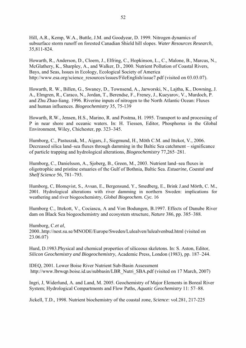
52

Hill, A.R., Kemp, W.A., Buttle, J.M. and Goodyear, D. 1999. Nitrogen dynamics of subsurface storm runoff on forested Canadian Shield hill slopes. Water Resources Research, 35,811-824. Howarth, R., Anderson, D., Cloern, J., Elfring, C., Hopkinson, L., C., Malone, B., Marcus, N., McGlathery, K., Sharpley, A., and Walker, D., 2000. Nutrient Pollution of Coastal Rivers, Bays, and Seas, Issues in Ecology, Ecological Society of America http://www.esa.org/science_resources/issues/FileEnglish/issue7.pdf (visited on 03.03.07).

Howarth, R. W., Billen, G., Swaney, D., Townsend, A., Jarworski, N., Lajtha, K., Downing, J. A., Elmgren, R., Caraco, N., Jordan, T., Berendse, F., Freney, J., Kueyarov, V., Murdoch, P. and Zhu Zhao-liang. 1996. Riverine inputs of nitrogen to the North Atlantic Ocean: Fluxes and human influences. Biogeochemistry 35, 75-139

Howarth, R.W., Jensen, H.S., Marino, R. and Postma, H. 1995. Transport to and processing of P in near shore and oceanic waters. In: H. Tiessen, Editor, Phosphorus in the Global Environment, Wiley, Chichester, pp. 323–345. Humborg, C., Pastuszak, M., Aigars, J., Siegmund, H., Möth C.M. and Ittekot, V., 2006. Decreased silica land–sea fluxes through damming in the Baltic Sea catchment – significance of particle trapping and hydrological alterations, Biogeochemistry 77,265–281. Humborg, C., Danielsson, A., Sjoberg, B., Green, M., 2003. Nutrient land–sea fluxes in oligotrophic and pristine estuaries of the Gulf of Bothnia, Baltic Sea. Estuarine, Coastal and Shelf Science 56, 781–793.

Humborg, C, Blomqvist, S., Avsan, E., Bergensund, Y., Smedberg, E., Brink J.and Mörth, C. M., 2001. Hydrological alterations with river damming in northern Sweden: implications for weathering and river biogeochemistry, Global Biogeochem. Cyc. 16

Humborg C., Ittekott, V., Cociascu, A and Von Bodungen, B.1997. Effects of Danube River dam on Black Sea biogeochemistry and ecosystem structure, Nature 386, pp. 385–388. Humborg, C.et al, 2000..http://nest.su.se/MNODE/Europe/Sweden/Lulealven/lulealvenbud.html (visited on 23.06.07) Hurd, D.1983.Physical and chemical properties of siliceous skeletons. In: S. Aston, Editor, Silicon Geochemistry and Biogeochemistry, Academic Press, London (1983), pp. 187–244. IDEQ, 2001. Lower Boise River Nutrient Sub-Basin Assessment http://www.lbrwqp.boise.id.us/subbasin/LBR_Nutri_SBA.pdf (visited on 17 March, 2007) Ingri, J, Widerlund, A. and Land, M. 2005. Geochemistry of Major Elements in Boreal River System; Hydrological Compartments and Flow Paths, Aquatic Geochemistry 11: 57–88. Jickell, T.D., 1998. Nutrient biochemistry of the coastal zone, Science: vol.281, 217-225

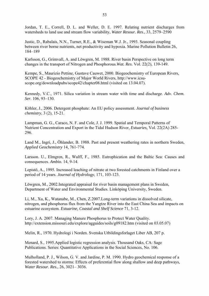
53

Jordan, T. E., Correll, D. L. and Weller, D. E. 1997. Relating nutrient discharges from watersheds to land use and stream flow variability, Water Resour. Res., 33, 2579–2590 Justic, D., Rabalais, N.N., Turner, R.E., & Wiseman W.J. Jr., 1993. Seasonal coupling between river borne nutrients, net productivity and hypoxia. Marine Pollution Bulletin 26, 184–189

Karlsson, G., Grimvall, A. and Löwgren, M. 1988. River basin Perspective on long term changes in the transport of Nitrogen and Phosphorous.Wat. Res. Vol. 22(2), 139-149.

Kempe, S., Maurizio Pettine, Gustave Cauwet, 2000. Biogeochemistry of European Rivers, SCOPE 42 - Biogeochemistry of Major World Rivers, http://www.icsu-scope.org/downloadpubs/scope42/chapter08.html (visited on 13.04.07). Kennedy, V.C., 1971. Silica variation in stream water with time and discharge. Adv. Chem. Ser. 106, 93–130. Köhler, J., 2006. Detergent phosphate: An EU policy assessment. Journal of business chemistry, 3 (2), 15-21. Lampman, G. G., Caraco, N. F. and Cole, J. J. 1999. Spatial and Temporal Patterns of Nutrient Concentration and Export in the Tidal Hudson River, Estuaries, Vol. 22(2A) 285-296. Land M., Ingri, J., Öhlander, B. 1988. Past and present weathering rates in northern Sweden, Applied Geochemistry 14, 761-774. Larsson. U., Elmgren, R., Wulff, F., 1985. Eutrophication and the Baltic Sea: Causes and consequences. Ambio. 14, 9-14. Lepistö, A., 1995. Increased leaching of nitrate at two forested catchments in Finland over a period of 14 years. Journal of Hydrology, 171, 103-123. Löwgren, M., 2002.Integrated appraisal for river basin management plans in Sweden, Department of Water and Environmental Studies. Linköping University, Sweden. Li, M., Xu, K., Watanabe, M., Chen, Z.2007.Long-term variations in dissolved silicate, nitrogen, and phosphorus flux from the Yangtze River into the East China Sea and impacts on estuarine ecosystem. Estuarine, Coastal and Shelf Science 71, 3-12. Lory, J. A. 2007. Managing Manure Phosphorus to Protect Water Quality. http://extension.missouri.edu/explore/agguides/soils/g09182.htm (visited on 03.05.07) Melin, R., 1970. Hydrologi i Norden. Svenska Utbildingsforlaget Liber AB, 207 p. Menard, S., 1995.Applied logistic regression analysis. Thousand Oaks, CA: Sage Publications. Series: Quantitative Applications in the Social Sciences, No. 106. Mulholland, P. J., Wilson, G. V. and Jardine, P. M. 1990. Hydro geochemical response of a forested watershed to storms: Effects of preferential flow along shallow and deep pathways, Water Resour. Res., 26, 3021– 3036.

54

Murdoch, P.S., Stoddard, J.L., 1992. The role of nitrate in the acidification of streams in the Catskill Mountain of New York, Water Resources Research .28, 2707-2720. Muylaert, K. and Raine, R.1999. Import, mortality and accumulation of coastal phytoplankton in a partially mixed estuary (Kinsale harbour, Ireland) Hydrobiology, 412, 53–65. Nedwell, D.B, Jickells, T.D., Trimmer, M. and Sanders, R. 1999. Nutrients in estuaries. In: D.B. Nedwell and D.G. Raffaelli, Editors, Estuaries. Adv. Ecol. Res. vol. 29, 43–92. NE.se (National Encyclopaedia of Sweden). http://www.ne.se/jsp/notice_board.jsp?i_type=1 (visited 15.07.07) Nixon, S. W., 1996. The fate of nitrogen and phosphorus at the land-sea margin of the North Atlantic Ocean. Biogeochemistry 35, 141–180. Officer, C. B., Biggs, R. B., Taft, J. L., Cronin, L. E., Tyler, M. & Boynton, W. R. (1984). Chesapeake Bay anoxia: origin, development, and significance. Science 223, 22-27. Official Statistics Sweden, 2002. (http://www.scb.se/templates/Publikation____193672.asp (visited on 15.09.07) Osmond, D.L., Line, D.E., Gale, J.A., Gannon, R.W., Knott, C.B., Bartenhagen, K.A., Turner, M.H, Coffey, S.W., Spooner, J., Wells, J., Walker, J.C.,. Hargrove, L.L., Foster, M.A., Robillard, P.D. and Lehning, D.W. 1995. WATERSHEDS: Water, Soil and Hydro-Environmental Decision Support System, http: //h2osparc.wq.ncsu.edu.(visited on 24.07.07 ) Peters, N. E. and Leavesley, G. H. 1995. Biotic and abiotic processes controlling water chemistry during snowmelt at Rabbit Ears Pass, Rocky Mountains, Colorado, Wat. Air Soil Pollut., 79, 171-190. Pitkänen, H., 1986. Discharges of nutrients and organic matter to the Gulf of Bothnia by Finnish rivers. National Board of Waters, Helsinki, Finland. Publications of the Water Research Institute, No. 68, 72-83. Pote, D. H., Daniel, T. C., Sharpley, A. N., Moore, P. A., Edwards, D. R., Nichols, D. J., 1996. Relating extractable soil phosphorus to phosphorus losses in runoff. Soil Sci. Soc. Am. J., 60, 855– 859. Probst, K. 2001.Temporal Variation in Silica and Alkalinity in Groundwater and Stream Water from White River Field Station near IUPUI, Indianapolis Indiana http://www.cees.iupui.edu/Research/Restoration/ARBOR/Publications/Reports_Projects/K-Probst_GeoChem_Report/Wells.pdf(visited on 01.05.07). Probst, J.L. 1985. Nitrogen and phosphorus exportation in the Garonne basin, France. Journal of Hydrology 76, 281-305. Qureshi, N. A., 1995.The role of faecal pellets in the flux of carbon to the sea floor on a river-influenced continental shelf subject to hypoxia. Ph.D. dissertation, Department of Oceanography and Coastal Sciences, Louisiana State University, Baton Rouge, Louisiana.

55

Raven J.A., Waite, A.M. 2004. The evolution of silicification in diatoms: inescapable sinking and sinking as escape. New Phytologist 162 (1), 45-61. Schelske, C. L., 1985. Biogeochemical silica mass balances in Lake Michigan and Lake Superior. Biogeochemistry 1, 197–218. Schloss, I.R., Ferreyra, G.A., Ruiz-Pino, D, 2002. Phytoplankton Biomass in Antarctic Shelf Zones: A conceptual model based on Potter Cove, King George Island. Journal of Marine Systems 36: 129-143 Seelig, B. and Nowatzki, J. 2001. Water Quality and Nitrogen, http://www.ag.ndsu.edu/pubs/h2oqual/watnut/ae1216w.htm (visited on 08.05.07) Semhi, K., Suchet, A. P., Clauer, N., Probst J.L., 2000. Impact of nitrogen fertilizers on the natural weathering erosion processes and the fluvial transport in the Garonne basin. Appl Geochem. 15, 865–878 SEPA, 2002. (http://www.internat.naturvardsverket.se/index.php3?main=/documents/nature/nacatego/araland/araland.htm (visited on 13.04.07) SEPA, 1997. http://www.internat.naturvardsverket.se/ (visited on 12.04.2007) SEPA, 1993. Eutrophication of the soil, fresh water and the sea, The Environment in Sweden-Status and Trends SIBER, 2002. www.siber.ecology.su.se (visited on 13.05.07) Sigleo, A. and Frick, W. 2002. Seasonal Variations in River Flow and Nutrient Concentrations in a North-western USA Watershed, U.S. Environmental Protection Agency, Ecosystems Research Division, Athens, GA 30605. Sileika, A. S., Kutra, S. and Berankiene, L. 2002. Phosphate run-off on the Nevezius River (Lithuania), Environmental Monitoring and Assessment 78, 153–167. Silva, M. A. L.; Calasans, C.F., Ovalle, A.R.C., and Rezende, C.E.(2001 ).Dissolved Nitrogen and Phosphorus Dynamics in the Lower Portion of the Paraiba do Sul River, Campos dos Goytacazes, RJ, Brazil, Braz. arch.biol.technol. vol.44 no.4 Curitiba Dec. 2001.http://www.scielo.br/scielo.php?script=sci_arttext&pid=S1516-89132001000400006&lng=in&nrm=iso&tlng=in Smayda, T. J., 1990. Novel and nuisance phytoplankton blooms in the sea: evidence for global epidemic. In Toxic Marine Phytoplankton (E. Graneli, B. Sundstrom, R. Edler & D. M. Anderson, eds.), pp. 29-40. Elsevier, New York. Smetacek, V. 1998. Biological oceanography: diatoms and the silicate factor. Nature, 391, 224-225. Smetacek, V. 1999. Diatoms and the ocean carbon cycle. Protist 150 (1), 25-32.

56

SMHI, 2003. http://www.smhi.se/sgn0102/n0204/vdragreg.pdf (visited on 13.05.07) SMHI, 2002. http://www.smhi.se/sgn0102/bhdc/xxx-stationlist/swe-stationlist.html(visited on 19 .06.07) SMHI, 1995. Weather and Water. En tidning från SMHI -Weather 1994, Norrköping. Swedish Meteorological and Hydrological Institute. ISSN 0281-9619 Smith, S.V., 1994. Phosphorus versus nitrogen limitation in the marine environment. Limnology and Oceanography, 29, 1149–1160. Smith, S. V.and Hollibaugh, J. T. 2003. Humans, hydrology and the distribution of inorganic nutrient loading to the ocean. Bioscience 53, 235–245. Soetaert, K., Middelburg, J. J. and Heip, C., Meire, P., Van Damme, S. and Maris, T. 2006.Long-term change in dissolved inorganic nutrients in the heterotrophic Scheldt estuary (Belgium, The Netherlands), Limnol. Oceanogr. 51(1, part 2), 409–423. Sommer, U. 1989. Nutrient status and nutrient competition of phytoplankton in a shallow hyper trophic lake. Limnol. Oceanogr. 34, 1173-1182 Stålnacke, P., 1996. Nutrient Loads to the Baltic Sea. The institute of Tema Research, Department of Water and Environment Studies, Linköping University, Linköping, Sweden. Stålnacke, P., Grimvall, A., Sundblad, K. and Wilander, A., 1999. Trends in nitrogen transport in Swedish rivers, Environ. Monit. Assess. 47–72. Tonderski, A., 1997. Control of nutrient fluxes in large river basins. PhD Thesis. Linköping University Studies in Arts and Science No. 157, Linköping, Sweden. Tranter, M., Tsiouris, S., Davies, T.D and Jones, H.G., 1992. A laboratory investigation of the leaching of solute from snow pack by rainfall. Hydrological Processes 6, 169–178. Ulén, B., Fölster, J.2007. Recent trends in nutrient concentrations in Swedish agricultural rivers, Science of the Total Environment 373, 473–487. Ume river homepage. 2004. http://www.umeriver.com/content/view/5/6/ (visited on 06-08-07) U.S. Geological Survey, 2001. Nutrients in the nations waters-too much of a good thing. National Water-Quality Assessment Program. USGS Circular- 1136. Vagstad N., Stålnacke, P., Andersson, H.E. and Tumas, R. 2004. Regional variation in diffuse nitrogen losses from agriculture in Nordic and Baltic Regions, Hydrology and Earth System Sciences 8(4), 651-662. Vought, L.B.M., Pinay, G., Fuglsang, A., Ruffinoni, C., 1995. Structure and function of buffer strips from a water quality perspective in agricultural landscapes. Landsc Urban Plan 31,323–331

57

Wallen, C.C., 1951. Nederborden i Sverige. Medelvarden 1901-1930. Meddelanden frin Sveriges Meteorologiska och Hydrologiska Institut. Ser. A. Nr. 4, 48 p. Geografiska Annaler. 70 A, 1-2 Walve, J. 2002. Nutrient limitation and elemental ratio in the Baltic Sea, Department of System Ecology, Stockholm University, Sweden. Wedepohl, K. H., 1969. Composition and abundance of common igneous rocks, in Handbook of Geochemistry, vol. 1, Edited by K. H. Wedepohl, pp. 227– 249, Springer-Verlag, New York. Wiederholt, R., Franzen D., Johnson, B., 2005.Livestock Manure Utilization in No-till Cropping Systems, NDSU, Extension service, North Dakota State University Fargo, North Dakota 58105 http://www.ag.ndsu.edu/pubs/ansci/waste/nm1292.pdf

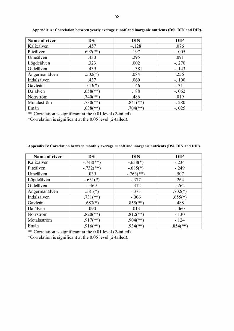
58

Appendix A: Correlation between yearly average runoff and inorganic nutrients (DSi, DIN and DIP). Name of river DSi DIN DIP Kalixälven .457 –.128 .076 Piteälven .692(**) .197 -. 005 Umeälven .430 .295 .091 Lögdeälven .323 .002 -. 270 Gideälven .439 – . 381 -. 143 Ångermanälven .502(*) .084 .256 Indalsälven .437 .060 -. 100 Gavleån .543(*) .146 -. 311 Dalälven .658(**) .188 -. 062 Norrström .740(**) .486 .019 Motalaström .730(**) .841(**) -. 280 Emån .638(**) .704(**) -. 025 ** Correlation is significant at the 0.01 level (2-tailed). *Correlation is significant at the 0.05 level (2-tailed). Appendix B: Correlation between monthly average runoff and inorganic nutrients (DSi, DIN and DIP).

Name of river DSi DIN DIP Kalixälven -.748(**) -,638(*) -,234 Piteälven -.732(**) -.685(*) -.249 Umeälven .039 -.763(**) .507 Lögdeälven -.631(*) -.377 .264 Gideälven -.469 -.312 -.262 Ångermanälven .581(*) -.373 .702(*) Indalsälven .731(**) -.006 .655(*) Gavleån .683(*) .855(**) .488 Dalälven .090 .013 -.060 Norrström .820(**) .812(**) -.130 Motalaström .917(**) .904(**) -.124 Emån .916(**) .934(**) .854(**) ** Correlation is significant at the 0.01 level (2-tailed). *Correlation is significant at the 0.05 level (2-tailed).

59

Appendix C: Graph showing residual analysis of DSi

-1,5 -1,0 -0,5 0,0 0,5 1,0 1,5

Standardized Predicted Value

-4

-2

0

2

4

Stan

dard

ized

Re

sidu

al

KalixälvenDependent Variable: DSi

R Sq Linear = 0,003

-2,0 -1,5 -1,0 -0,5 0,0 0,5 1,0

Standardized Predicted Value

-2

0

2

4

Stan

dard

ized

Re

sidu

al

PiteälvenDependent Variable: DSi

R Sq Linear = 0

-4 -2 0 2 4

Standardized Predicted Value

-2

0

2

4

6

Stan

dard

ized

Re

sidu

al

UmeälvenDependent Variable: DSi

R Sq Linear = 1,11E-16

-2 -1 0 1 2

Standardized Predicted Value

-4

-2

0

2

4

Stan

dard

ized

Re

sidu

alLögdeälven

Dependent Variable: DSi

R Sq Linear = 0,003

-2 -1 0 1 2

Standardized Predicted Value

-3

-2

-1

0

1

2

3

4

Stan

dard

ized

Re

sidu

al

GideälvenDependent Variable: DSi

R Sq Linear = 2,114E-4

-3 -2 -1 0 1 2 3 4

Standardized Predicted Value

-2

0

2

4

6

Stan

dard

ized

Re

sidu

al

ÅngermanälvenDependent Variable: DSi

R Sq Linear = 0

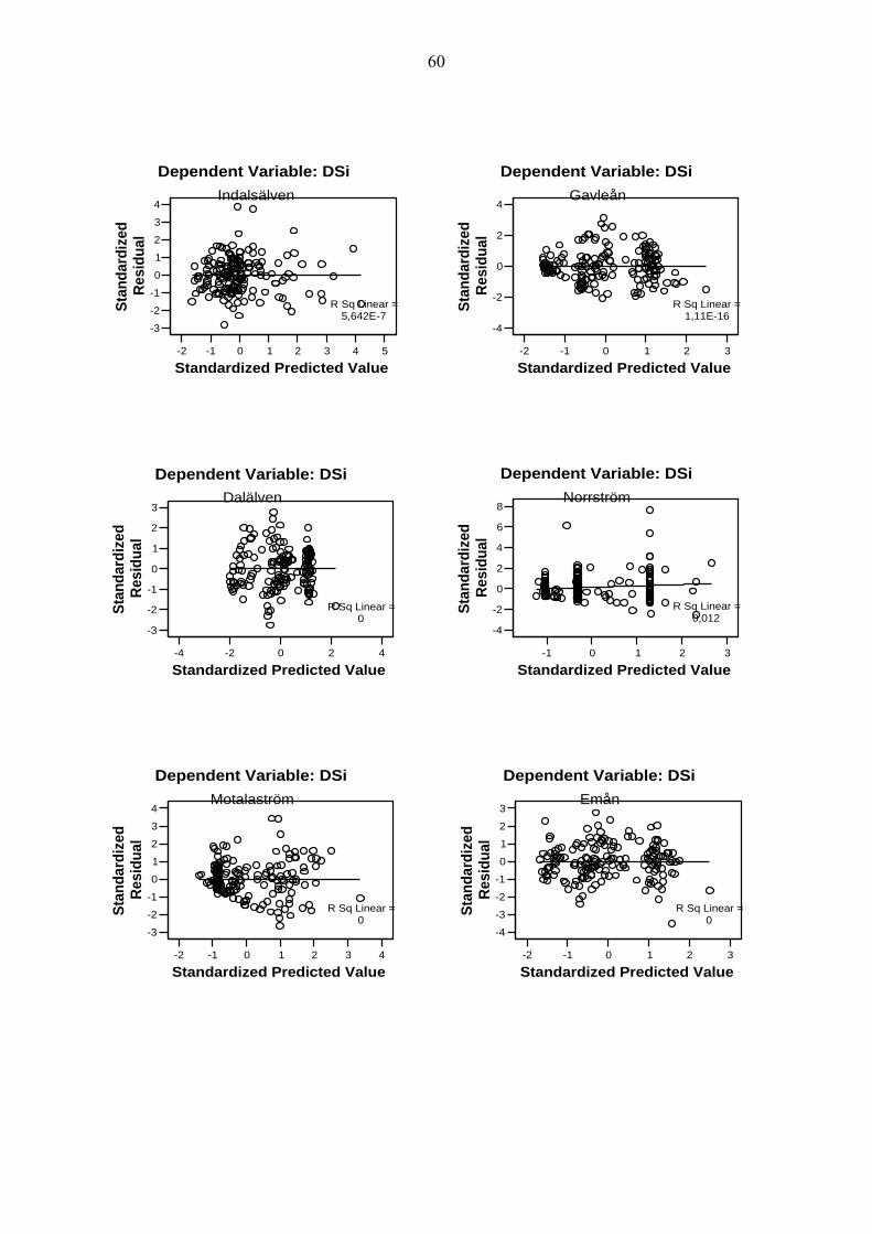
60

-2 -1 0 1 2 3 4 5

Standardized Predicted Value

-3

-2

-1

0

1

2

3

4

Stan

dard

ized

Re

sidu

al

IndalsälvenDependent Variable: DSi

R Sq Linear = 5,642E-7

-2 -1 0 1 2 3

Standardized Predicted Value

-4

-2

0

2

4

Stan

dard

ized

Re

sidu

al

GavleånDependent Variable: DSi

R Sq Linear = 1,11E-16

-4 -2 0 2 4

Standardized Predicted Value

-3

-2

-1

0

1

2

3

Stan

dard

ized

Re

sidu

al

DalälvenDependent Variable: DSi

R Sq Linear = 0

-1 0 1 2 3

Standardized Predicted Value

-4

-2

0

2

4

6

8

Stan

dard

ized

Re

sidu

alNorrström

Dependent Variable: DSi

R Sq Linear = 0,012

-2 -1 0 1 2 3 4

Standardized Predicted Value

-3

-2

-1

0

1

2

3

4

Stan

dard

ized

Re

sidu

al

MotalaströmDependent Variable: DSi

R Sq Linear = 0

-2 -1 0 1 2 3

Standardized Predicted Value

-4

-3

-2

-1

0

1

2

3

Stan

dard

ized

Re

sidu

al

EmånDependent Variable: DSi

R Sq Linear = 0

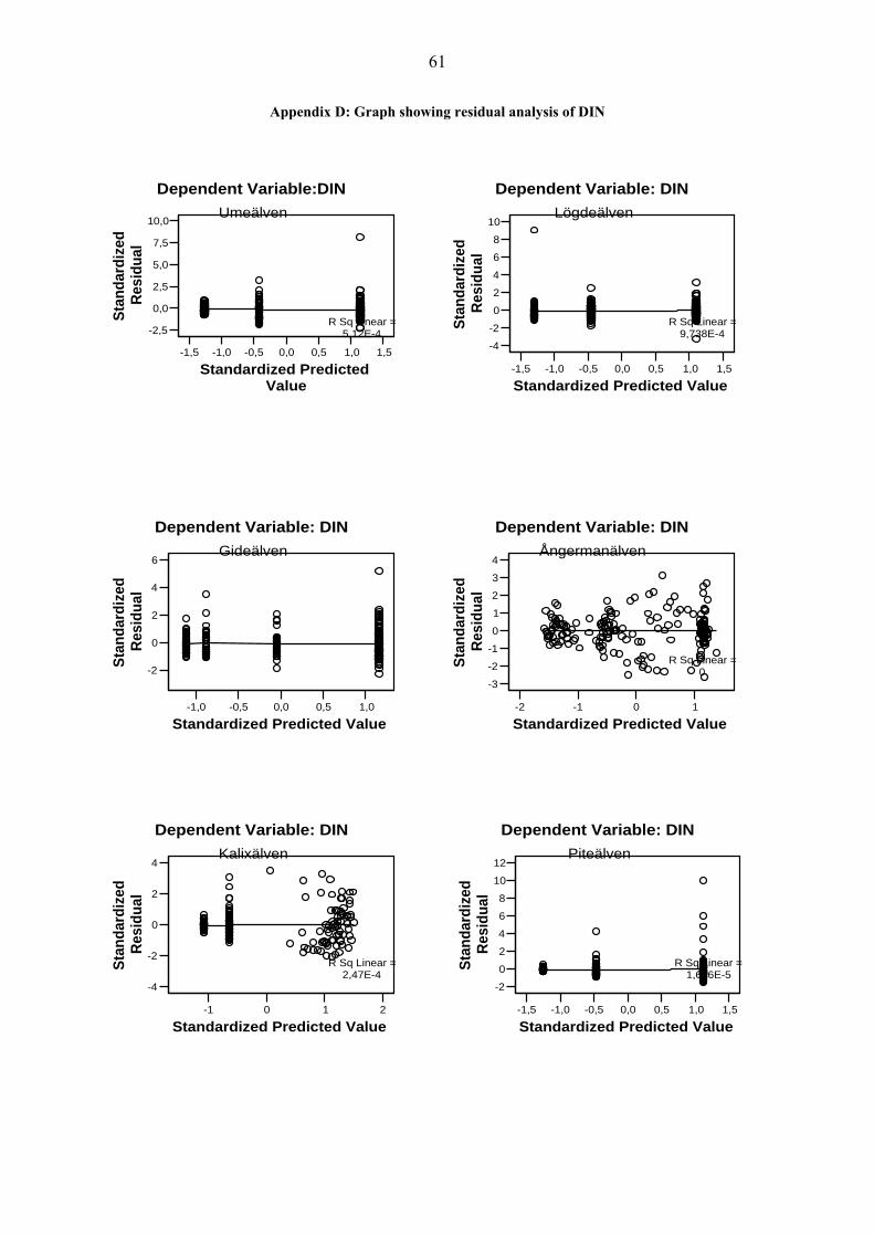
61

Appendix D: Graph showing residual analysis of DIN

-1,5 -1,0 -0,5 0,0 0,5 1,0 1,5

Standardized Predicted Value

-2,5

0,0

2,5

5,0

7,5

10,0

Stan

dard

ized

Re

sidu

al

UmeälvenDependent Variable:DIN

R Sq Linear = 5,12E-4

-1,5 -1,0 -0,5 0,0 0,5 1,0 1,5

Standardized Predicted Value

-4

-2

0

2

4

6

8

10

Stan

dard

ized

Re

sidu

al

LögdeälvenDependent Variable: DIN

R Sq Linear = 9,738E-4

-1,0 -0,5 0,0 0,5 1,0

Standardized Predicted Value

-2

0

2

4

6

Stan

dard

ized

Re

sidu

al

GideälvenDependent Variable: DIN

-2 -1 0 1

Standardized Predicted Value

-3

-2

-1

0

1

2

3

4

Stan

dard

ized

Re

sidu

al

ÅngermanälvenDependent Variable: DIN

R Sq Linear = 0

-1 0 1 2

Standardized Predicted Value

-4

-2

0

2

4

Stan

dard

ized

Re

sidu

al

KalixälvenDependent Variable: DIN

R Sq Linear = 2,47E-4

-1,5 -1,0 -0,5 0,0 0,5 1,0 1,5

Standardized Predicted Value

-2

0

2

4

6

8

10

12

Stan

dard

ized

Re

sidu

al

PiteälvenDependent Variable: DIN

R Sq Linear = 1,616E-5

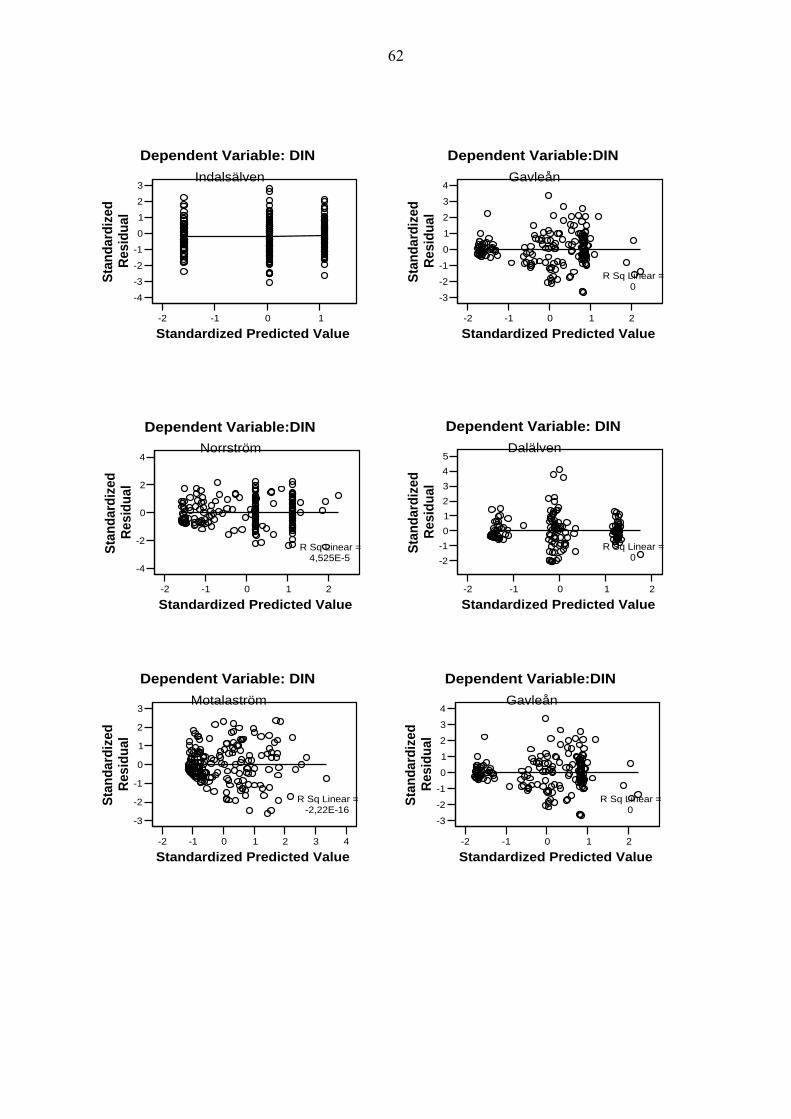
62

-2 -1 0 1

Standardized Predicted Value

-4

-3

-2

-1

0

1

2

3

Stan

dard

ized

Re

sidu

al

IndalsälvenDependent Variable: DIN

-2 -1 0 1 2

Standardized Predicted Value

-3

-2

-1

0

1

2

3

4

Stan

dard

ized

Re

sidu

al

GavleånDependent Variable:DIN

R Sq Linear = 0

-2 -1 0 1 2

Standardized Predicted Value

-4

-2

0

2

4

Stan

dard

ized

Re

sidu

al

NorrströmDependent Variable:DIN

R Sq Linear = 4,525E-5

-2 -1 0 1 2

Standardized Predicted Value

-2-1012345

Stan

dard

ized

Re

sidu

alDalälven

Dependent Variable: DIN

R Sq Linear = 0

-2 -1 0 1 2 3 4

Standardized Predicted Value

-3

-2

-1

0

1

2

3

Stan

dard

ized

Re

sidu

al

MotalaströmDependent Variable: DIN

R Sq Linear = -2,22E-16

-2 -1 0 1 2

Standardized Predicted Value

-3

-2

-1

0

1

2

3

4

Stan

dard

ized

Re

sidu

al

GavleånDependent Variable:DIN

R Sq Linear = 0

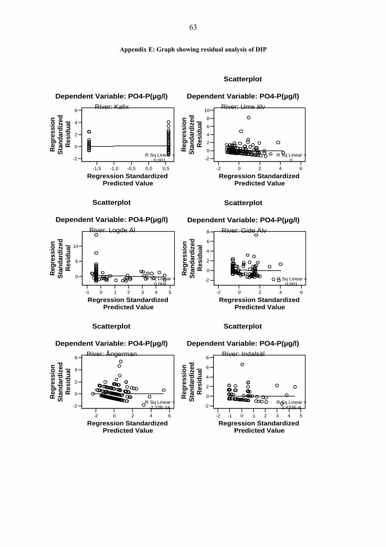
63

Appendix E: Graph showing residual analysis of DIP

-1,5 -1,0 -0,5 0,0 0,5

Regression Standardized Predicted Value

-2

0

2

4

6

Regr

essi

on

Stan

dard

ized

Re

sidu

al

River: KalixDependent Variable: PO4-P(µg/l)

R Sq Linear = 0,001

-2 0 2 4 6

Regression Standardized Predicted Value

-2

0

2

4

6

8

10

Regr

essi

on

Stan

dard

ized

Re

sidu

al

River: Ume älvDependent Variable: PO4-P(µg/l)

Scatterplot

R Sq Linear = 0

-1 0 1 2 3 4 5

Regression Standardized Predicted Value

0

5

10

Regr

essi

on

Stan

dard

ized

Re

sidu

al

River: Logde ÄlDependent Variable: PO4-P(µg/l)

Scatterplot

R Sq Linear = 0,004

-2 0 2 4 6

Regression Standardized Predicted Value

-2

0

2

4

6

8

Regr

essi

on

Stan

dard

ized

Re

sidu

al

River: Gide ÄlvDependent Variable: PO4-P(µg/l)

Scatterplot

R Sq Linear = 0,001

-2 0 2 4 6

Regression Standardized Predicted Value

-2

0

2

4

6

Regr

essi

on

Stan

dard

ized

Re

sidu

al

River: ÅngermanDependent Variable: PO4-P(µg/l)

Scatterplot

R Sq Linear = -2,22E-16

-2 -1 0 1 2 3 4 5

Regression Standardized Predicted Value

-2

0

2

4

6

8

Regr

essi

on

Stan

dard

ized

Re

sidu

al

River: IndalsälDependent Variable: PO4-P(µg/l)

Scatterplot

R Sq Linear = 2,433E-8

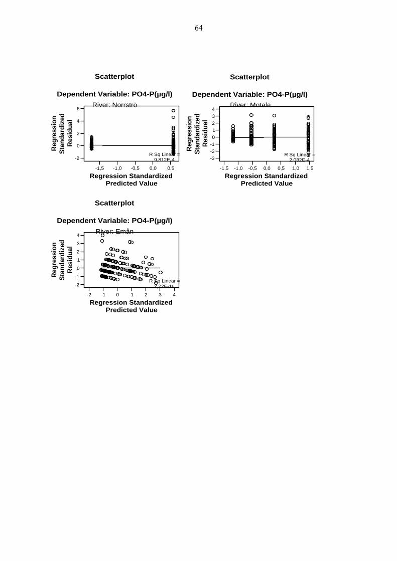
64

-1,5 -1,0 -0,5 0,0 0,5

Regression Standardized Predicted Value

-2

0

2

4

6

Regr

essi

on

Stan

dard

ized

Re

sidu

al

River: NorrströDependent Variable: PO4-P(µg/l)

Scatterplot

R Sq Linear = 9,812E-4

-1,5 -1,0 -0,5 0,0 0,5 1,0 1,5

Regression Standardized Predicted Value

-3-2-101234

Regr

essi

on

Stan

dard

ized

Re

sidu

al

River: MotalaDependent Variable: PO4-P(µg/l)

Scatterplot

R Sq Linear = 2,082E-4

-2 -1 0 1 2 3 4

Regression Standardized Predicted Value

-2

-1

0

1

2

3

4

Regr

essi

on

Stan

dard

ized

Re

sidu

al

River: EmånDependent Variable: PO4-P(µg/l)

Scatterplot

R Sq Linear = 2,22E-16