QEDQueen’s Economics Department Working Paper No. 257

Seasonality in Regression:An Application of Smoothness Priors

Mark GersovitzPrinceton University

James G. MacKinnonQueen’s University

Department of EconomicsQueen’s University

94 University AvenueKingston, Ontario, Canada

K7L 3N6

1-1977

Seasonality in Regression:An Application of Smoothness Priors

Mark Gersovitz

Department of EconomicsPrinceton UniversityPrinceton, NJ 08540

U.S.A.

and

James G. MacKinnon

Department of EconomicsQueen’s University

Kingston, Ontario, CanadaK7L 3N6

Abstract

This article argues that conventional approaches to the treatment of seasonality ineconometric investigation are often inappropriate. A more appropriate technique is toallow all regression coefficients to vary with the season, but to constrain them to doso in a smooth fashion. A Bayesian method of estimating smoothly varying seasonalcoefficients is developed, based on Shiller’s (1973) approach to estimating distributedlags. In a sampling experiment, this technique outperforms ordinary least squares by asubstantial margin. An application of this technique to the estimation of the demandfor soft drinks is also presented.

The authors would like to thank R. J. Arnott, C. M. Beach, P. T. Chinloy, J. W. Eaton, M. C.

Lovell, three referees, and R. E. Quandt for helpful comments on earlier drafts. This paper

was published in the Journal of the American Statistical Association, 73, 1978, 264–273.

January, 1977

1. Introduction

Many economic time series display regular seasonal fluctuations. If the seasonal fluc-tuations in the independent variables fully accounted for the seasonal fluctuations inthe dependent variables, no problem would exist for econometricians. Indeed, by im-parting additional variation to the independent variables, seasonal fluctuations wouldincrease the precision of coefficient estimates. It is often the case, however, that whenseasonally varying dependent variables are regressed on seasonally varying independentvariables, the resulting residuals have a seasonal pattern. Faced with this situation, thepracticing econometrician typically does one of two things: Either he inserts dummyvariables to capture the effects of seasonality, or he employs seasonally adjusted data(usually provided by official sources). In this article, a third approach is advocated.We propose to allow all of the parameters of the model to vary from season to season,but to constrain them to do so in a smooth fashion.

The rationale for this approach is developed in this section. An estimation procedurewhich implements the approach is presented in Section 2. The results of some samplingexperiments which investigate the performance of this procedure are given in Section 3.Finally, in Section 4, the technique is applied to the estimation of the demand for softdrinks in Canada.

The economic model which explains an economic time series x(t) may be written as

x(t) = f(z(t), u(t), θ

), (1.1)

where z(t) is a vector of other economic time series, which may include lagged values,including lagged values of x(t) itself, u(t) is a vector of random errors, and θ is avector of parameters. In some cases, it may be possible to rewrite (1.1) as

x(t) = g(z(t), u(t),θ1

)+ S(t,θ2). (1.2)

That is, it may be possible to break x(t) into two parts, one of which (S) variessystematically with the season but does not depend on z(t), and the other of which (g)does not show any systematic seasonal variation. Of course, x(t) may be the logarithmof a series, so that (1.2) would actually be a multiplicative relationship. If the modelcan be written in this way, we say that it displays separable seasonality; if not, we saythat it displays inseparable seasonality. If deseasonalization of the time series x(t) isto be practical, the model underlying x must display separable seasonality. Otherwise,one could not hope to estimate θ2 independently of θ1, and hence a deseasonalizedseries could not be arrived at without first estimating (1.1).

Many techniques for deseasonalization have been proposed; see, among others, Lovell(1963), Jorgenson (1964), Shiskin, Young, and Musgrave (1967), and Sims (1974).It should be noted that inserting seasonal dummies into a regression on raw datais equivalent to using one of these standard deseasonalization techniques; see Lovell(1963). All such techniques attempt to estimate the seasonal component without

–1–

estimating, or even knowing the form of, equation (1.1). Thus they all assume thatseasonality is separable.

Economic theory, however, provides no support for this assumption. The one unifyingprinciple of neoclassical theory is that market behavior should be derived from under-lying tastes and technology by assuming that agents maximize some quantity such asutility or profits. Thus seasonal variation in market variables should be derived fromseasonal influences on tastes and technology. It is easy to construct simple modelsof this type, and we have investigated a number of them. In every case where theutility, cost, or production functions were realistic, the demand or supply functionsderived from them displayed inseparable seasonality. Thus we believe that inseparableseasonality is the rule rather than the exception for economic time series.

In principle, the econometrician should use economic theory to specify the functionalforms of the relationships he or she estimates, including the ways in which seasonalfactors enter into them. In practice, however, partly because most theory applies to in-dividual agents while most time series data apply to broad aggregates, microeconomictheory provides little guidance about functional forms. The econometrician typicallyfalls back on some variant of the general linear model to serve as an approximation ofthe true functional form which is complicated and unknown. If seasonality is not sepa-rable, this approximation should be different in every season, so that every parameteris allowed to vary from season to season. Thus an appropriate model to estimate is

yt =λ∑

i=1

DitXtβi + εt, (1.3)

where yt is a dependent variable and Xt is a vector of independent variables at time t,Dit is a scalar equal to unity if t is in the ith season and equal to zero otherwise, βi isa vector of coefficients for season i, and the number of seasons is λ.

The model (1.3) is simply a generalization of the traditional dummy variable procedurein which all parameters, not merely the intercept, are allowed to vary seasonally. Henceit can approximate a true functional form in which seasonality is inseparable. Ordinaryleast squares estimation of (1.3) is equivalent to simply fitting a separate relationshipfor every season, and thus it is likely to lead to rather imprecise estimates unless thesample size is large. One would, therefore, like to impose some additional restrictionson the model. In many situations, it may be reasonable to impose the restriction thatthe values of each parameter in adjacent seasons will not differ greatly. We refer tothis as the assumption of smooth seasonality. It is often a useful assumption, and inthe next section we present a technique for its econometric implementation. First,however, we examine the smooth seasonality hypothesis more closely.

Three objections may be raised to the assumption that parameters vary smoothlyfrom season to season. First, such an assumption is simply inappropriate in somesituations. For example, the demand for Easter eggs varies seasonally, but the variationis probably not very smooth, and, moreover, it will be different in different years. Insuch situations, the smooth seasonality assumption should not be employed.

–2–

Second, the smooth seasonality hypothesis puts no restrictions on relationships amongthe coefficients on different variables. Unfortunately, such restrictions are not, ingeneral, justified. Consider the utility function

U(x1, sx2), (1.4)

where x1 and x2 are the quantities of goods 1 and 2, and s is a parameter whichvaries smoothly with the season. If the functional form of U were unknown, onewould often estimate log-linear relationships between quantities demanded, prices,and income, in which the parameters of interest are price and income elasticities. Itcan straightforwardly be shown that when demand functions are derived from (1.4),the effect of a change in s on the income elasticity of the demand for each good isquite different from the effect of such a change on the price elasticities. Thus therelationships among coefficients on different variables can be expected to vary withthe season.

A final objection is that phenomena which are usually called seasonal are often directlylinked to one or more dimensions of the weather, such as temperature or rainfall.Thus one should incorporate weather directly into the model to explain seasonality.Such a proposal is attractive in principle, but it may be very hard to implement.Weather has many dimensions and often varies enormously across regions for whichstatistical data are available. Thus it is doubtful that seasonality could be adequatelyexplained by only a few weather variables. Even if it could be, it seems likely that theparameters of the model would depend on the weather variable(s) in a complicated andnonlinear way, so that specifying the model might be very difficult. Moreover, someseasonal phenomena may depend not so much on actual weather as on the weatherthat usually occurs in those seasons, so that use of weather data may introduce anerrors-in-variables problem. The hypothesis of smoothly varying seasonal parametersmay be regarded as a way of approximating the effects of average weather on themodel’s parameters. In Section 4, where we present an example of our smoothnesstechnique, we also examine methods for the explicit use of weather data.

2. Seasonally Varying Parameters and Smoothness Priors

The problem of estimating parameters which vary with the season is not unlike theproblem of estimating a distributed lag model. In both cases, the main difficulty isthe large number of parameters that could potentially be estimated, and the obvioussolution is to constrain the estimates in some way, The most elegant and flexibletechnique for constraining the coefficients of a distributed lag is the Bayesian techniquerecently proposed by Shiller (1973). In this section, his technique is adapted to thecase of seasonally varying parameters; where possible, Shiller’s notation is used.

A natural constraint to impose is that the coefficients of a given variable should varysmoothly across the seasons. Depending on what is meant by “smoothly,” this re-quirement could imply that the first, second, or higher differences should be small.The technique proposed here could be used to impose any of these constraints. To

–3–

conserve space, only first degree smoothness priors (which impose constraints on thesecond differences) are considered here.

For simplicity, consider the case with only one independent variable. Suppose that

yt =λ∑

i=1

βiDitxt + εt, (2.1)

where xt and yt are scalar time series at time t, Dit = 1 if t is in the ith season, andDit = 0 otherwise. For a first degree smoothness prior, second differences between theseasonally varying coefficients are assumed to be small. That is

(βi − βi−1)− (βi−1 − βi−2) = βi − 2βi−1 + βi−2 (2.2)

is assumed to be small for all periods i. Note that the periodicity of the seasons impliesthat the first coefficient is linked to the last as well as to the second; thus βi−1 = βλ

if i = 1, and so on.

The second differences of the vector β may be written as

u = R1β, (2.3)

where R1 is a λ × λ matrix which generates (2.2). For example, when λ = 4 (i.e.,when the data are quarterly),

R1 =

1 −2 1 00 1 −2 11 0 1 −2−2 1 0 1

. (2.4)

In Shiller’s development, the prior information that the second differences are small isrepresented by assuming that the second differences are normally and independentlydistributed with mean zero and variance ζ2. Hence u comes from a spherical normaldistribution with covariance matrix ζ2I. In the case of seasonally varying coefficients,however, this simple formulation is inadmissible, because the second differences arelinearly dependent. This fact is easily verified by noting that the first λ − 1 rows ofR1 sum to minus the λth row.

Since the second differences of β are linearly dependent, the prior information thatthey are small presumably cannot be represented by the assumption that they arenormally and independently distributed (but see the following discussion). Instead,we specify that they are normally distributed with a variance-covariance matrix whichis consistent with their being linearly dependent. The simplest formulation for thevariance-covariance matrix of u which takes into account the particular form of thislinear dependence is

ζ2Ω = ζ2

1 ω ω · · · ω ωω 1 ω · · · ω ω...

......

......

ω ω ω · · · ω ωω ω ω · · · ω 1

, (2.5)

–4–

where ω = −1/(λ−1), and Ω is λ×λ. Since |Ω| = 0, u has a degenerate distribution.Therefore, from now on, we deal with the distribution of u∗, which is equal to u withthe last element deleted. Define R∗

1 as a (λ− 1)× λ matrix consisting of R1 with thelast row deleted. Then

u∗ = R∗1β, (2.6)

and u∗ is normally distributed with covariance matrix ζ2Ω∗, where Ω∗ is derived bydeleting the last row and last column of Ω. Finally, define

R1 = Ω∗−1/2R∗1 (2.7)

andu = R1β. (2.8)

The vector u has a spherical normal distribution with covariance matrix ζ2Iλ−1.

In order to impose a prior on u, it is necessary to know Ω∗−1/2 From the form ofΩ, it is obvious that this must be a matrix with α1 on the principal diagonal and α2

everywhere else. Solving for α1 and α2 is straightforward. There are two solutions,one of which is

α1 =λ + λ1/2 − 2

(λ− 1)1/2λ1/2, α2 =

λ1/2 − 1(λ− 1)1/2λ1/2

. (2.9)

This solution may be derived from a formula provided by Nerlove (1971).

The matrix R1 plays exactly the same role as Shiller’s R1. Thus combining the prioron u with a normal likelihood function for the εt, which are assumed to be n.i.d. withvariance σ2, yields a posterior distribution which is normal. The smoothness estimatorof β is given by

β = (X>X)−1X>y, (2.10)

where

X ≡[

D1x D2x · · ·Dλx

kR1

], (2.11)

y ≡[

y

0

], (2.12)

andk ≡ σ/ζ. (2.13)

Obtaining β is considerably easier if one replaces kR1 in (2.11) by

(λ− 1

λ

)1/2

kR1 (2.14)

–5–

and lengthens the vector of zeros in y accordingly. It is proved in Appendix 1 that β isunaffected by this substitution.1 It is easy to obtain β using an ordinary least-squaresregression package; it is merely necessary to add λ zeros to the vector y, and the λrows of R1, multiplied by (

(λ− 1)/λ)1/2

k,

to the X matrix. This procedure can thus be interpreted in the context of mixedestimation, in a manner analogous to Taylor’s (1974) interpretation of Shiller’s proce-dure. If k is large, the dummy observations will carry a lot of weight, and as a resultthe estimated second differences will be small. The choice of k will be discussed inSection 3.

The procedure outlined above can be extended directly to the case where there ismore than one independent variable. A different prior must be specified for each set ofseasonally varying coefficients, and hence a different k must be used for each. If thereare T observations and n variables, all with seasonally varying coefficients, then Xwill have nλ columns and T + nλ rows, with λ rows of dummy observations for eachof the n variables.

3. Sampling Experiments

Several sampling experiments were performed to investigate the performance of thesmooth seasonality technique. The main objectives of these experiments were to seehow the smoothness technique compares with ordinary least squares, and to find outhow the choice of k affects the estimates.

The model examined is

yt =12∑

i=1

aiDit +12∑

i=1

biDitxt + ut, (3.1)

where Dit is a dummy variable that equals one when t equals i plus an integer multipleof 12, and that equals zero elsewhere. The error term ut is normally distributed withmean zero and variance σ2. The independent variable xt is generated by

xt =12∑

i=1

ciDit(Art) + et, (3.2)

where et has mean zero and variance σ2e . Thus xt trends upward but also varies

seasonally (due to the ci) and randomly.

1 We are grateful to an anonymous referee for pointing this out to us. It may alsobe noted that our procedure is equivalent to using an Aitken estimator on the com-plete stacked regression, with the Moore-Penrose generalized inverse of the variance-covariance matrix Ω.

–6–

In the sampling experiments reported here, the following parameter values were used:

c1 = c2 = c3 = 0.9,

c4 = c5 = c6 = c10 = c11 = c12 = 1.0,

c7 = c8 = c9 = 1.1,

A = 10, r = 1.005, σe = 1,

a1 = 8, a2 = 8, a3 = 9, a4 = 10a5 = 10, a6 = 11,

a7 = 12, a8 = 12, a9 = 11, a10 = 10, a11 = 10, al2 = 9,

b1 = 1.173205, b2 = 1.1, b3 = 1.0, b4 = 0.9, b5 = 0.826795, b6 = 0.8,

b7 = 0.826795, b8 = 0.9, b9 = 1.0, b10 = 1.1, b11 = 1.173205, b12 = 1.2

(3.3)

Note that the bi follow a sinusoidal pattern. They were in fact generated by theequation

bi = 1.0 + 0.2 cos(πi/6).

The pattern of the ai, though regular, is somewhat less smooth.

The correct values of ka and kb are σ/ζa and σ/ζb, respectively. But although σ isknown, ζa and ζb, the standard deviations of the priors on the second differences ofthe ai and the bi, are not. Since the assumed ai and bi were not actually generatedas realizations of multivariate normal distributions on their second differences, theirstandard deviations are not good estimators of ζa and ζb. Shiller suggests that, forthe distributed lag case, ζ should be derived by assuming that the lag has a vee shapeand the sum of coefficients expected by the investigator. An analogous procedure forthe seasonal case is to assume that the seasonal coefficients follow a vee wave, withthe true (or expected) amplitude, rising linearly for half the year and falling linearlyfor the other half. One could also assume that the coefficients lie on a square wavewith given amplitude, so that they are equal to their largest value for half the yearand to their smallest for the other half. Given some such set of assumed βi, one maycompute the value of ζ using

ζ2 =β>R∗

1>Ω∗−1R∗

1β

λ− 1, (3.4)

or, equivalently from Appendix 1,

ζ2 = β>R1>R1β/λ. (3.5)

Expression (3.4) has the form of a maximum likelihood estimate of ζ2, and (3.5) issimply the mean of the squared second differences of the elements of β.

If the ai follow a vee wave with their actual amplitude, the resulting value of ζa

is 0.544331, and if they follow a square wave, the resulting value of ζa is 2.309401;similar assumptions on the bi, which have one-tenth the amplitude, yield values of ζb

one-tenth as large. These values of ζa and ζb were used in the sampling experiments.

–7–

The square wave assumption yields relatively small values of k, and the vee waveassumption yields relatively large values of k, so the two estimators will be referred toas the small-k and large-k estimators, respectively.

The results from two sampling experiments are presented in Tables 1 and 2. In bothcases, the model was given by (3.1), (3.2), and (3.3), the number of observations was120 (corresponding to ten years of monthly data), and the number of replicationswas 100. These simulations were written in FORTRAN on a Burroughs B6700, using48-bit floating point arithmetic. The error terms were generated by a routine whichapproximates a normally distributed random variate by the sum of twelve pseudo-random uniform variates. In the two experiments reported on here, the standarddeviation of the error term in (3.1), σ, is 0.5 and 1.0, respectively. Different values ofσ were investigated because, as σ increases, the weight accorded the prior informationalso increases.

Root mean square errors (RMSE) are presented in columns one to three of Tables 1and 2. Note that a refers to the average of the ai, so that the entries in columns 1to 3 beside a refer to the RMSE of the average, while the entries beside “avg.” referto the average of the RMSEs over the 12 periods. It is evident from Table 1 that thesmoothness estimators have substantially lower RMSEs than ordinary least-squares(OLS) estimators; the only coefficients for which the difference is not substantial are aand b. The large-k RMSEs are somewhat smaller than the small-k RMSEs; however,the former are much more variable than the latter. The results in Table 2 confirmthose in Table 1, the main difference being that all RMSEs are substantially larger,and the relative performance of OLS is worse.

Mean biases are presented in columns four through six of Tables 1 and 2. An aster-isk indicates that bias was significant at the 5 percent level, according to a simplenonparametric test on the number of replications for which the estimate exceeded thetrue value; critical points were 39 and 61 replications, using the normal approxima-tion to the binomial. The small-k estimates exhibit some bias, but it is not large andmainly affects a few coefficients. The large-k estimates, on the other hand, exhibitvery substantial bias, especially for σ = 1.0. The estimates apparently tend to reducethe amplitude of the true seasonal coefficients; large coefficients are underestimated,and small ones are overestimated.

Experiments for larger values of σ, not reported here, confirm the results suggested bycomparing Tables 1 and 2: As the standard error of the regression increases, the RMSEsof the smoothness estimates increase. When σ is very large, the large-k estimatesexhibit almost no seasonal variation at all, and the small-k estimates are substantiallybiased.

It should be remembered that, in all these experiments, k was set equal to σ/zeta,so that the weights on the dummy observations increased linearly with σ. It wouldappear to be the case that, in order to avoid excessive bias, k should vary less thanproportionately with σ.

–8–

4. An Application

To illustrate how the smooth seasonality technique performs in practice, it was appliedto the estimation of the demand for soft drinks in Canada, using monthly data. Themodel estimated is

Ct =12∑

i=1

Dit(a1iSt + a2iSDPt + a3iFPt + a4iEXt + a5iYt) + ut, (4.1)

where Ct is the log of per capita soft drink consumption, St = 1, SDPt is the log of theprice of soft drinks relative to a nonfood price index, FPt is the log of the price of foodrelative to the nonfood price index, EXt is the log of per capita real expenditure, andYt is a variable representing the relative proportion of young people in the population.The index i is one in January. Monthly data for 1959:1 to 1974:6 are employed, so thatthere are 186 observations. Since all variables are measured in natural logarithms, thecoefficients are elasticities. Precise definitions of all variables are given in Appendix 2.This model is presented here as an illustration of technique, not as a definitive analysisof soft drink demand.

The values of k1 through k5 for this example were chosen as follows. First, OLS wasapplied to equation (4.1). The ζj were then computed from (3.5) on the assumptionthat the j th coefficients had mean equal to the mean of the OLS coefficients andfollowed a square wave which varied from +100 percent to −100 percent of that mean.The quantity kj was then computed as σ/ζj , where σ is the estimated standard errorfrom the OLS regression. This procedure yielded the following values for the kj :

k1 = 0.0111, k2 = 0.0822, k3 = 0.2466, k4 = 0.0123, k5 = 0.1206.

For purposes of comparison, two more restrictive models were also estimated. One,which will be referred to as “Lovell”, because it uses the dummy-intercept treatmentof seasonality dealt with by Lovell (1963), constrains aji to equal aj for all variablesexcept the intercept. The second, which will be referred to as “Unified”, constrainsaji to equal aj for all variables, and thus takes no account of seasonality at all.

The results of smoothness estimation of (4.1) with the kj given above, of OLS es-timation of (4.1), and of the Lovell and Unified models, are presented in Table 3.Numbers in parentheses are t statistics. The Unified model is clearly inappropriate.Its estimates are wildly different from those of the other three models, its R2 is verylow, and an F test of Unified against OLS rejects the former at all normal significancelevels. The Lovell model is not as clearly inappropriate; OLS fits significantly betterthan it does at the ten percent level, but not at the five percent level. This doessuggest, however, that it would be dangerous to accept the Lovell model as a completetreatment of seasonality in soft drink demand. There is no evidence of twelfth-orderautocorrelation for either the Lovell or Smoothness models, according to a regression ofthe residuals on those lagged twelve months. In contrast, Unified displays evidence of

–9–

severe twelfth-order autocorrelation (significant at more than the .01 level), suggestingthat this test on the residuals is a useful diagnostic.

In terms of the estimates of average coefficients, there is little to choose between theSmoothness, OLS, and Lovell approaches. However, the Lovell approach necessar-ily gives no information about the seasonal pattern of the coefficients, and the OLSestimates jump around so much that they also provide no useful information. TheSmoothness estimates, on the other hand, generally vary from month to month in asimple, regular fashion. Thus, if the investigator has any interest in the seasonal pat-tern of the coefficients, either because it is interesting in itself or because it may provideevidence of misspecification (if, for example, the peaks are in the wrong season), thesmoothness technique would appear to be well worth employing.

One way to test the appropriateness of the smoothness restrictions is to use Theil’stest for the compatibility of prior and sample information (Theil 1971, pp. 350–351).Under the null hypothesis, the test statistic is distributed as a chi-squared randomvariable with 55 degrees of freedom. The value of the statistic for the prior we usedis 197.9, which is more than twice the 0.005 tail value. Thus the sample informationappears to be inconsistent with the smoothness prior. It should be noted, however,that if the kj are reduced by a factor of two, the resulting priors, which seemed to ustoo weak, do pass the Theil test at the .05 level.

As discussed in Section 2, an alternative to the seasonally varying parameters modelis the explicit introduction of weather into the regression. The dimension of weathermost relevant to soft drink demand is temperature. Accordingly, we introduced atemperature variable, Wt, which is a weighted average of daily maximum temperaturesin Canada’s three largest metropolitan areas, in or near which most Canadians live;see Appendix 2.

Initially, we simply added Wt to the specification, either additively or multiplicatively.The results were disappointing. Neither Wt nor Wt times each of the five other vari-ables added significantly to the explanatory power of OLS applied to (4.1). Althoughthey did add significantly to the power of the Unified model, the resulting equationswere not very impressive.

We then experimented with a spline approach (Poirier, 1975) to allow for nonlineareffects. We felt that 35 F might represent a temperature below which changes intemperature would have no effect on the demand for soft drinks, while 70 F mightrepresent a temperature beyond which changes in temperature would greatly affectdemand. Accordingly, we defined

W1 =

W − 35 if W ≥ 350 otherwise

andW2 =

W − 70 if W ≥ 700 otherwise.

The spline approach worked considerably better than using just a single weather vari-able. Adding W1 and W2 to equation (4.1) reduced the SSR from 0.5411 to 0.5113, a

–10–

reduction which is significant at the .05 level; the F statistic is 3.613, compared withF.05(2, 124) = 3.069. Adding W1 and W2 times each of the other variables reducedthe SSR to 0.4580, a reduction which is also significant; the F statistic is 2.104, com-pared with F.05(10, 116) = 1.913. Thus the weather variables do appear to add to thespecification.

The weather variables alone, however, do not perform nearly as well as OLS. Themodel

Ct =5∑

j=1

ajXjt + b1W1t + b2W2t + ut (4.2)

had an SSR of 1.7396. Adding the seasonal variables of (4.1) yielded an F statistic of5.416, compared with F.05(55, 116) = 1.445. Thus the seasonally-varying parametersadd considerably to the specification based on the weather variables. Using seasonally-varying coefficients alone seems preferable to using (4.2) or (4.3). It would appearthat, in this case, the explicit introduction of weather variables cannot replace theseasonally-varying parameters model, but it may be a useful addition.

5. Conclusion

We have argued that the mechanical treatment of seasonality by the use of deseasonal-ized data or seasonal dummies cannot, in general, be justified on the basis of economictheory. Econometricians should, instead, attempt to build seasonality into their mod-els. If that is not possible, they should at least allow seasonal influences to enter inless restrictive ways than is customary. One way to do so is to allow all coefficientsto vary with the season, but OLS estimation of such models is likely to be difficult.An alternative approach involving the use of smoothness priors is described here, andsampling experiments show that it compares well with OLS. The smoothness approachwas then applied to estimating the demand for soft drinks, and it performed well com-pared with the explicit use of weather variables. The smooth seasonality approachthus appears to be practical and potentially useful.

–11–

Appendix 1

This appendix shows that β is unchanged if kR1 in (2.11) is replaced by

((λ− 1)/λ

)1/2kR1,

and the number of zeros in Y is correspondingly increased by one. The only part of(2.10) which is affected by the substitution is X>X, which is originally equal to

X>X + k2R∗1>Ω∗−1R∗

1 (A.1)

and becomesk2

((λ− 1)/λ

)R1>R1. (A.2)

The inverse of Ω∗ is a matrix with 2(λ− 1)/λ on the principal diagonal and (λ− 1)/λeverywhere else. Thus the second term in (A.1) can be written as

k2((λ− 1)/λ

)R∗

1>WR∗

1, (A.3)

where W is a matrix with 2 on the principal diagonal and 1 everywhere else.

Let M be a matrix consisting of an identity matrix of order λ− 1 plus an additionalrow every element of which is −1. It is easily seen that

R1 = MR∗1, (A.4)

since the identity matrix simply recreates R∗1 and the final row of restores the last row

of R1, which is equal to minus the sum of the rows of R∗1. Moreover, it may readily

be verified that M>M = W. Hence

R∗1>WR∗

1 = R∗1>M>MR∗

1 = R1>R1. (A.5)

Thus the second term in (A.1) is equal to the second term in (A.2), which implies thatβ is unchanged.

–12–

Appendix 2

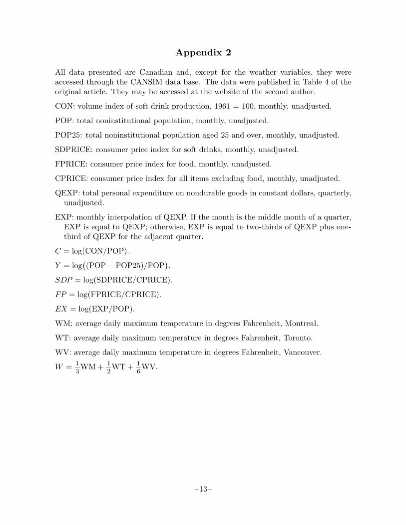
All data presented are Canadian and, except for the weather variables, they wereaccessed through the CANSIM data base. The data were published in Table 4 of theoriginal article. They may be accessed at the website of the second author.

CON: volume index of soft drink production, 1961 = 100, monthly, unadjusted.

POP: total noninstitutional population, monthly, unadjusted.

POP25: total noninstitutional population aged 25 and over, monthly, unadjusted.

SDPRICE: consumer price index for soft drinks, monthly, unadjusted.

FPRICE: consumer price index for food, monthly, unadjusted.

CPRICE: consumer price index for all items excluding food, monthly, unadjusted.

QEXP: total personal expenditure on nondurable goods in constant dollars, quarterly,unadjusted.

EXP: monthly interpolation of QEXP. If the month is the middle month of a quarter,EXP is equal to QEXP; otherwise, EXP is equal to two-thirds of QEXP plus one-third of QEXP for the adjacent quarter.

C = log(CON/POP).

Y = log((POP− POP25)/POP

).

SDP = log(SDPRICE/CPRICE).

FP = log(FPRICE/CPRICE).

EX = log(EXP/POP).

WM: average daily maximum temperature in degrees Fahrenheit, Montreal.

WT: average daily maximum temperature in degrees Fahrenheit, Toronto.

WV: average daily maximum temperature in degrees Fahrenheit, Vancouver.

W = 1−3WM + 1−

2WT + 1−

6WV.

–13–

References

Jorgenson, Dale W. (1964). “Minimum variance, linear, unbiased seasonaladjustment of economic time series,” Journal of the American StatisticalAssociation, 59, 681–724.

Lovell, Michael C. (1963). “Seasonal adjustment of economic time series andmultiple regression analysis,” Journal of the American Statistical Association, 58,993–1010.

Nerlove, Marc (1971). “A note on error component models,” Econometrica, 39,383–396.

Poirier, Dale J. (1976). The Econometrics of Structural Change, Amsterdam:North-Holland.

Shiller, Robert J. (1973). “A distributed lag estimator derived from smoothnesspriors,” Econometrica, 41, 775–789.

Shiskin, Julius, Young, Allan H., and Musgrave, John C. (1967). The X-11 Variantof the Census Method II Seasonal Adjustment Program, Bureau of the CensusTechnical Paper No. 15 (revised), Washington, D.C.: U.S. Department ofCommerce.

Sims, Christopher A. (1974). “Seasonality in regression,” Journal of the AmericanStatistical Association, 69, 618–626.

Taylor, William E. (1974). “Smoothness priors and stochastic prior restrictions indistributed lag estimation,” International Economic Review, 15, 803–804.

Theil, Henri (1971). Principles of Econometrics, New York: John Wiley & Sons.

–14–

Table 1. First Experiment: σ = 0.5

RMSE Bias

Coef. OLS Small-k Large-k OLS Small-k Large-k

a1 0.9326 0.6411 0.6759 −0.1551 0.0398 0.5185∗

a2 1.1687 0.6637 0.6116 −0.1602 0.0160 0.4310∗

a3 0.8696 0.6244 0.4335 0.0545 −0.0646 −0.0691

a4 1.1716 0.7285 0.6318 −0.1051 −0.2572∗ −0.4533∗

a5 0.8122 0.6119 0.4317 −0.0370 0.0383 −0.0422

a6 1.1086 0.6855 0.5520 −0.2192 −0.1354 −0.3365∗

a7 0.8375 0.6520 0.8213 −0.1408 −0.2366∗ −0.7025∗

a8 0.8932 0.6970 0.7330 −0.0517 −0.1765 −0.5971∗

a9 0.9914 0.6445 0.3956 −0.1440 −0.0540 −0.0711

a10 0.9142 0.6326 0.4862 −0.0019 0.1334 0.3122∗

a11 0.8380 0.5489 0.3893 0.0238 −0.0861 −0.1043∗

a12 0.8303 0.5892 0.4432 0.1914 0.0709 0.1735∗

a 0.3015 0.2922 0.2915 −0.0621 −0.0593 −0.0784

avg. 0.9473 0.6433 0.5504

b1 0.07545 0.05177 0.05191 0.01434∗ −0.00137 −0.03841∗

b2 0.09541 0.05449 0.04930 0.01271 −0.00155 −0.03318∗

b3 0.06941 0.05050 0.03590 −0.00597 0.00365 0.00328

b4 0.08513 0.05237 0.04298 0.00705 0.01773∗ 0.02791∗

b5 0.06233 0.04685 0.03339 0.00361 −0.00170 0.00918

b6 0.07783 0.04690 0.03725 0.01503 0.00909 0.02406∗

b7 0.05565 0.04365 0.05332 0.00889 0.01515∗ 0.04480∗

b8 0.05848 0.04566 0.04785 0.00495 0.01295 0.03879∗

b9 0.06743 0.04561 0.02962 0.00951 0.00369 0.00517

b10 0.06200 0.04247 0.03084 0.00110 −0.00790 −0.01639∗

b11 0.05599 0.03702 0.02559 −0.00051 0.00653 0.00361

b12 0.05685 0.04041 0.03215 −0.01498 −0.00674 −0.01441∗

avg. 0.06850 0.04648 0.03918

–15–

Table 2. Second Experiment: σ = 1.0

RMSE Bias

Coef. OLS Small-k Large-k OLS Small-k Large-k

a1 1.6017 0.9848 1.2296 0.0959 0.2887 1.0634∗

a2 2.1140 1.0642 1.0884 −0.2663 0.2191∗ 0.8867∗

a3 1.8798 1.0819 0.6567 0.0890 −0.0565 0.1393∗

a4 1.9409 0.9474 0.8047 0.1671 −0.2639∗ −0.5174∗

a5 1.5108 0.9078 0.6719 0.0085 0.1083 −0.2819∗

a6 1.9447 1.0204 1.0177 −0.3095 −0.1110 −0.7945∗

a7 1.5287 1.0025 1.4186 −0.0663 −0.3127∗ −1.2691∗

a8 1.5233 0.9126 1.2388 0.0568 −0.2110 −1.0719∗

a8 2.2307 1.0511 0.6841 0.0448 0.1358 −0.2623∗

a9 1.7255 1.1010 0.7674 0.0960 0.3437∗ 0.4245∗

a10 1.9102 1.0111 0.6706 0.1146 −0.0854 0.1696

a11 1.8139 0.9894 0.8982 0.1027 0.0616 0.6310∗

a12 0.5102 0.5063 0.5074 0.0111 0.0097 −0.0735∗

avg. 1.8103 1.0062 0.9289

b1 0.13244 0.08351 0.09148 −0.00639 −0.02162∗ −0.07681∗

b2 0.17255 0.08866 0.08155 0.02045 −0.01866 −0.06554∗

b3 0.14595 0.08242 0.04850 −0.00845 0.00316 −0.01628∗

b4 0.13823 0.06696 0.05207 −0.01210 0.01781∗ 0.02538∗

b5 0.11459 0.07022 0.05589 −0.00398 −0.01007 0.03209∗

b6 0.13864 0.07124 0.07009 0.01657 0.00257 0.05518∗

b7 0.09613 0.06281 0.08630 0.00106 0.01698∗ 0.07609∗

b8 0.09499 0.05835 0.07455 −0.00608 0.01099 0.06246∗

b9 0.14290 0.06802 0.04626 −0.00360 −0.00948 0.01842∗

b10 0.11981 0.07612 0.04767 −0.00448 −0.02036 −0.01622∗

b11 0.12997 0.06993 0.04960 −0.00291 0.00929 −0.01932∗

b12 0.12692 0.06995 0.06681 −0.00632 −0.00357 −0.04705∗

b 0.03535 0.03504 0.03449 −0.00136 −0.00191 0.00237

avg. 0.12943 0.07235 0.06423

–16–

Table 3. Estimates of Soft Drink Demand

Variable Month Smoothness OLS Lovell Unified

S 1 −5.19 (7.64) −6.65 (5.34) −5.42 (15.64)

2 −4.69 (7.10) −3.45 (2.93) −5.30 (15.26)

3 −4.97 (7.73) −5.78 (4.96) −5.40 (15.53)

4 −4.81 (7.70) −4.44 (3.93) −5.22 (14.99)

5 −4.58 (7.46) −4.58 (4.18) −5.17 (14.87)

6 −4.70 (7.72) −3.97 (3.75) −4.98 (14.37)

7 −5.07 (7.82) −6.91 (5.95) −4.92 (14.29)

8 −5.10 (7.59) −4.12 (3.44) −4.95 (14.18)

9 −5.66 (8.24) −4.46 (3.51) −5.16 (14.54)

10 −6.16 (8.87) −8.72 (6.86) −5.42 (15.04)

11 −5.31 (7.62) −3.70 (2.80) −5.31 (14.94)

12 −5.16 (7.44) −4.66 (3.68) −5.25 (14,95)

avg. −5.12 −5.12 −5.21 −2.92 (3.99)

SDP 1 −0.65 (2.64) −0.72 (2.00)

2 −0.08 (0.32) 0.22 (0.58)

3 −0.45 (1.62) −0.52 (1.22)

4 −0.63 (2.18) −0.94 (2.10)

5 −0.63 (2.14) −0.30 (0.65)

6 −0.80 (2.69) −1.10 (2.37)

7 −1.01 (3.26) −0.66 (1.32)

8 −1.09 (3.50) −1.21 (2.43)

9 −1.16 (3.71) −1.48 (2.92)

10 −1.07 (3.50) −0.85 (1.80)

11 −0.62 (2.08) −0.53 (1.07)

12 −0.73 (2.83) −0.88 (2.39)

avg. −0.74 −0.69 −0.69 (5.31) −0.88 (2.58)

FP 1 0.24 (0.95) −0.14 (0.26)

2 0.14 (0.57) 0.27 (0.54)

3 0.08 (0.32) −0.05 (0.11)

4 0.06 (0.24) −0.11 (0.21)

5 0.08 (0.34) 0.49 (1.00)

6 0.09 (0.39) −0.17 (0.37)

7 0.19 (0.73) 0.21 (0.36)

8 0.29 (1.11) 0.54 (0.93)

9 0.36 (1.38) 0.39 (0.71)

10 0.40 (1.53) 0.26 (0.46)

11 0.37 (1.47) 0.25 (0.48)

12 0.34 (1.36) 0.89 (1.68)

avg. 0.22 0.23 0.17 (1.14) 1.01 (2.69)

Table continued on next page.

–17–

Table 3 (continued). Estimates of Soft Drink Demand

Variable Month Smoothness OLS Lovell Unified

EX 1 3.46 (2.31) 6.63 (2.60)

2 3.28 (2.20) 0.21 (0.09)

3 4.26 (2.98) 5.80 (2.54)

4 4.84 (3.52) 5.00 (2.21)

5 3.35 (2.36) 2.07 (0.90)

6 4.58 (3.25) 4.25 (1.92)

7 4.91 (3.18) 7.94 (3.25)

8 4.96 (3.33) 3.01 (1.27)

9 6.33 (4.39) 4.72 (1.97)

10 6.54 (4.79) 10.69 (4.69)

11 4.49 (3.17) 1.52 (0.64)

12 4.12 (2.81) 3.15 (1.29)

avg. 4.59 4.59 4.76 (6.86) −0.10 (0.08)

Y 1 0.41 (1.25) −0.22 (0.36)

2 0.64 (2.00) 1.09 (1.90)

3 0.67 (2.10) 0.32 (0.55)

4 0.74 (2.36) 1.05 (1.83)

5 0.64 (2.10) 0.45 (0.81)

6 0.61 (1.99) 1.12 (2.05)

7 0.35 (1.11) −0.58 (1.00)

8 0.37 (1.13) 0.81 (1.34)

9 0.34 (1.00) 0.99 (1.54)

10 0.19 (0.57) −1.04 (1.63)

11 0.39 (1.13) 1.10 (1.63)

12 0.40 (1.20) 0.64 (1.05)

avg. 0.48 0.47 0.43 (2.45) 1.42 (3.51)

SSR 0.6422 0.5411 0.7833 5.8110

R2 (unadjusted) 0.9107 0.9248 0.8911 0.1921

DW Statistic 2.043 1.844 1.963 0.859

Note: The t statistics for the Smoothness estimates are conditional on the prior.

–18–