82 DOI: 10.21608/pserj.2019.18192.1011

PORT-SAID ENGINEERING RESEARCH JOURNAL

Faculty of Engineering - Port Said University

Volume 24 No. 1 March 0202 pp: 82:101

(Marine Engineering)

Seawater Desalination Using Waste Heat Recovery on Passenger Ship Kandil, H.A., Hussein, A.W.

(1)

ABSTRACT:

This paper presents a study for sea water desalination on board of passenger ships using waste heat from the engine. Three

thermal methods for water desalination were explored, namely Forward Feed Multiple Effect Evaporation, Once Through

Multi-Stage Flash, and Brine Circulation Multi-Stage Flash. Computer simulation has been developed to calculate the

parameters of the desalination plant; the required amount of fresh water and the corresponding total heat transfer area. The

optimum plant selection is the one which achieves the required distillate flow rate with minimum heat transfer area. The effect

of different variables on the plant selection has been studied, i.e. steam temperature, exhaust temperature, and intake water

flow rate. An existing passenger ship has been selected to examine the proposed method where the optimum desalination

method has been selected for her using the developed software. To assess the effectiveness of the proposed method, the

economical, environmental, and technical gains are numerically analyzed. Using the waste heat recovery leads to reducing the

unit product cost of freshwater by circa 30%. The plant reduced the emissions by about five thousand tons of CO2, 100 tons of

NOx and 35 tons of SO2 per year. Applying the optimum design of the proposed salt water desalination on the case study saved

2.7 $/ m3 as a minimum comparing to the average cost of fresh water in ports. These savings can cover the plant capital cost in

six years at most.

Keywords: Desalination, Water generation, Waste heat recovery, Passenger ship

1. INTRODUCTION

In 2003, B. R. Smalley, (1996 Noble Laureate in

Chemistry) defined the humanity’s top ten problems for

the next 50 years [1]. Energy and water exist on the top of

his list. The challenge of permanently providing clean,

safe, and fresh water is the key of life. While the dilemma

of fuel price and availability is an inevitable fact. For

passenger ships, fresh water usually represents a high

percentage of the dead weight [2]. The average water

consumption per person in new ships rises to more than

300 liters per day [3]. The above facts lead directly to the

concept of sea water desalination on board passenger

ships. This will lead in a direct way to the reduction of

dead weight and the cost of purchasing water.

(1) Dept. of Naval Architecture & Marine

Engineering Port Said University, 42523- Port

Said, Egypt 1049-001 Lisboa, Portugal``

Water desalination is usually done by one of two

methods; membrane methods and thermal methods. The

thermal process is one of the oldest desalination methods

which are based on water evaporation. Fresh water is

formed when the condensate vapor is formed while the

brine remains with high concentration and usually thrown

back to the sea. Since the thermal methods require source

of energy, the waste heat from the engine can be used as

this source. This improves the efficiency of the engine,

reduces the emissions and creates an environmental

friendly system for water generation without using extra

energy source.

Fresh water generation on shipboard is indeed not

novel, but it has been applied on many shipboards

especially on passenger ships. Morsy et al. [4] proposed

fresh water generator onboard passenger ship which uses

the waste heat recovered from scavenging air to provide

the heat required to evaporate sea water. The proposed

system minimizes the fresh water supply by 8 tons/day; an

amount sufficient for 20 persons per day. Based on the

fact that the brine which passes to over board and the

steam will stay condensate in the steam condenser

converting into fresh water. It was recommended to use

brine in heating purpose or use this losses energy in next

study.

83

Mehner and Penney [5] presented a full-scale

shipboard system that incorporates multimedia filtration

and ultra-filtration, yet requires minimal space and optimal

power usage. This study received the first place award

given by the US Navy in a competition made to improve

the pretreatment for shipboard Reverse Osmosis potable

water system. The annual savings were $17,000, which

resulted in a payback period of 14 years.

In 2015, Guler el al. [6] studied the Reverse Osmosis,

RO system capability under different conditions together

with cost analysis examination on a relatively small cruise

ship. The system used had a daily water treatment capacity

of 30 m3. The study revealed that the used system is

capable of meeting the needs of the drinking and potable

water. Cost-wise, the resulting water was more costly

compared to water supply costs on land, as the above

authors expected in the beginning of the research.

Therefore, the authors recommended that one should

evaluate alternative energy sources, such as solar, wind or

wave energy for seawater desalination.

Grand Princess Cruise ship was the largest and most

expensive passenger ship ever built in 1998. The ship,

which uses more than 260,000 gallons of fresh water per

day, has implemented evaporator management programs

aimed at optimizing the operation of fresh water

evaporators by utilizing the waste heat generated by the

ships engines. The cooling water passed through these

engines is re-used to heat the salt water in the evaporators

[7].

The aim behind this paper is to study the sea water

desalination onboard passenger ship using thermal

methods. This goal is done using the waste heat from

engine as an energy source for the desalination plant.

Desalination is made by three methods, namely; the

Forward Feed Multiple Effect Evaporation (MEE-FF),

Once Through Multi Stage Flash (MSF-OT) and Brine

Circulation Multi Stage Flash (MSF-BC).

A computer simulation has been developed to calculate

the heat transfer area required for fresh water desalination

unit on ship board based on the required water demand.

The program is calibrated versus another research results

to confirm its validity. MS Freedom of the sees ship has

been selected to examine the proposed method. The

program is used to find the optimum specification of water

desalination plant fitted onboard the ship. Besides, it is

also used to study the effect of different variables on the

distillate flow rate and the total area of the plant.

Eventually, the optimum desalination method is selected

for the candidate ship; which gives the required water

demand for minimum heat transfer area.

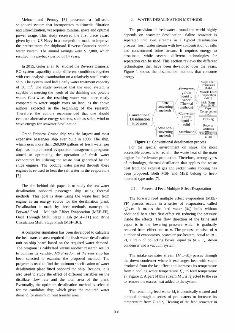
2. WATER DESALINATION METHODS

The provision of freshwater around the world highly

depends on seawater desalination. Saline seawater is

separated into two streams in a typical desalination

process; fresh water stream with low concentration of salts

and concentrated brine stream. It requires energy to

desalinate, while several different technologies for

separation can be used. This section reviews the different

technologies that have been developed over the years.

Figure 1 shows the desalination methods that consume

energy.

Figure 1: Conventional desalination process

For the special environment on ships, the most

accessible access is to reclaim the waste heat of the main

engine for freshwater production. Therefore, among types

of technology, thermal distillation that applies the waste

heat from the exhaust gas and jacket water cooling has

been proposed. Both MSF and MEE belong to heat-

operated type units [7].

2.1. Foreword Feed Multiple Effect Evaporation

The forward feed multiple effect evaporation (MEE-

FF) process occurs in a series of evaporators, called

effects. It makes the feed water (Mf) boils without

additional heat after first effect via reducing the pressure

inside the effects. The flow direction of the brine and

vapor is in the lowering pressure which is gradually

reduced from effect one to n. The process consists of n

number of evaporators, seawater pre-heaters, equal to (n –

2), a train of collecting boxes, equal to (n – 1), down

condenser and a vacuum system.

The intake seawater stream (Mcw+Mf) passes through

the down condenser where it exchanges heat with vapor

produced from the last effect and increases its temperature

from a cooling water temperature Tcw to feed temperature

Tf, Figure 2. A part of this stream Mcw is rejected to the sea

to remove the excess heat added to the system.

The remaining feed water Mf is chemically treated and

pumped through a series of pre-heaters to increase its

temperature from Tf to t2. Heating of the feed seawater in

Conventional Desalination

Processes

State converting methods

Converting from

liquid to vapor

(Thermal methods)

Single Effect Evaporation

(SEE)

Multiple Effect

Evaporation (MEE)

Multi Stage Flash (MSF)

Vapor

Compression (VC) Convertin

g from liquid to

solid

Freasing

State non-converting methods

Membrane

Reverse Osmosis

(RO) Electrodialysi

s (ED)

84

the pre-heaters is made by condensing the flashed off

vapor from the effects dj and the collecting boxes dj\. The

feed water is sprayed over the outside surface of the first

evaporator tubes. The brine temperature rises to the

boiling temperature T1 which corresponds to the pressure

of the vapor space. The vapor formed in the first effect

flows as heating vapor to the second effect. The non-

evaporated seawater from the first effect B1 enters the

second effect as feed water. From the second effect

onward, freshwater is produced inside the effect by two

different mechanisms; boiling Dj and flashing dj [8,9].

Motive steam Ms, extracted from an external source drives

vapor formation in the first effect [10].

2.2. Brine Circulation Multi Stage Flash

The multistage flashing desalination units (MSF) are

typically constructed with large capacity that may vary

from 50,000 to 75,000 m3/d. This capacity is almost 2–3

times the conventional units installed in 1980’s [11]. The

process is based on the principle of flash evaporation, as

seawater is evaporated by reducing the pressure due to

raising the temperature.

In MSF distillation process vapor formation takes

place within the liquid bulk instead of the surface of hot

tubes. The hot brine is allowed to freely flow and flash in

a series of chambers; this feature keeps the hot and

concentrated brine from the inside or outside surfaces of

heating tubes. This is a major advantage over the original

concept of thermal evaporation, where submerged tubes of

heating steam are used to perform fresh water evaporation.

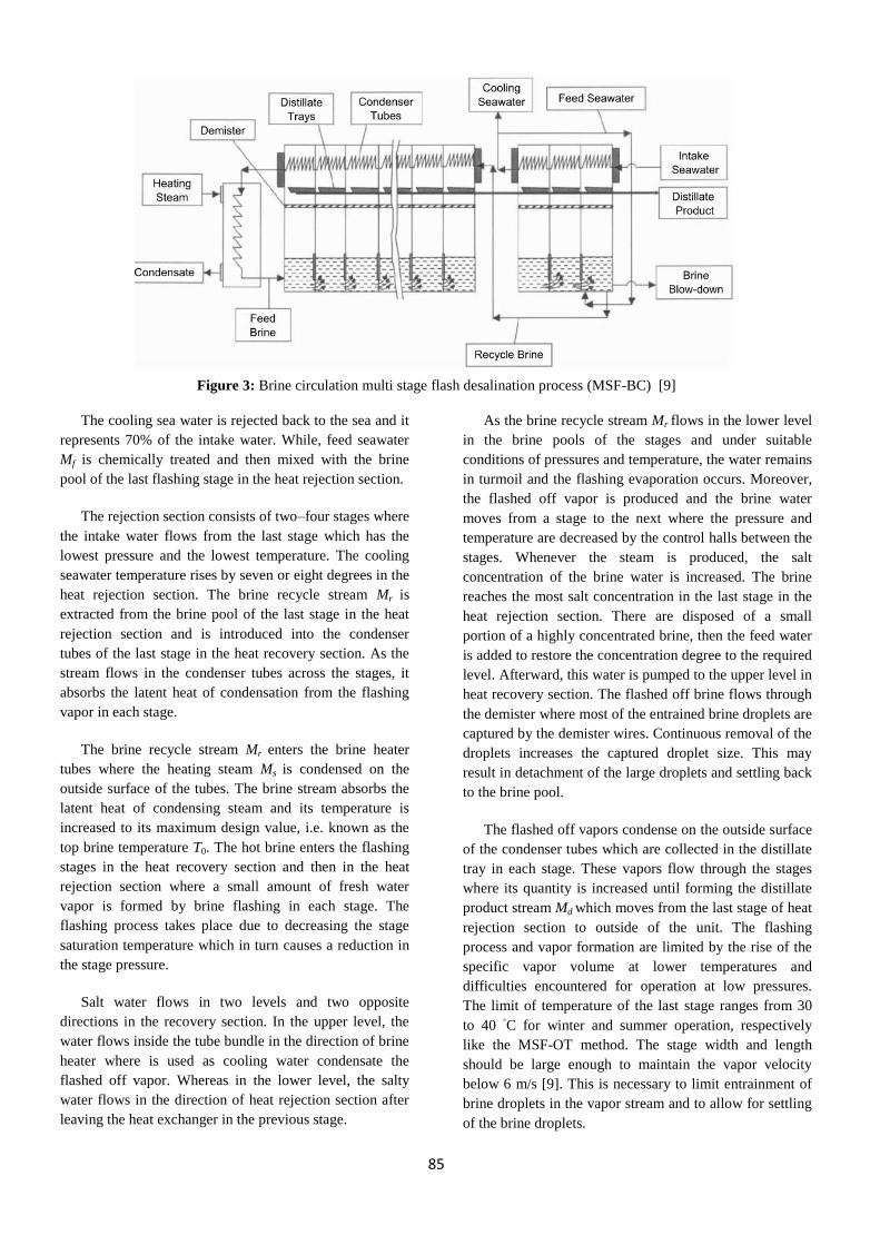
The process elements are illustrated in Figure 3 where

the flashing stages are divided among the heat recovery

and heat rejection sections. The main aim of adding heat

rejection section is to control the temperature of the intake

seawater and to reject the excess heat added in the brine

heater. This process starts with the brine heater and

finishes with the rejection section and between them there

is recovery section that consists of a set of evaporation

stages.

The intake seawater stream Mf + Mcw is introduced into

the condenser tubes of the heat reject section where its

temperature is increased by absorbing the latent heat of the

condensing fresh water vapor. The warm stream of intake

seawater is divided into two parts; cooling seawater Mcw

and feed seawater Mf .

Figure 2: Conventional of a MEE process (forward feed configuration) [8]

85

Figure 3: Brine circulation multi stage flash desalination process (MSF-BC) [9]

The cooling sea water is rejected back to the sea and it

represents 70% of the intake water. While, feed seawater

Mf is chemically treated and then mixed with the brine

pool of the last flashing stage in the heat rejection section.

The rejection section consists of two–four stages where

the intake water flows from the last stage which has the

lowest pressure and the lowest temperature. The cooling

seawater temperature rises by seven or eight degrees in the

heat rejection section. The brine recycle stream Mr is

extracted from the brine pool of the last stage in the heat

rejection section and is introduced into the condenser

tubes of the last stage in the heat recovery section. As the

stream flows in the condenser tubes across the stages, it

absorbs the latent heat of condensation from the flashing

vapor in each stage.

The brine recycle stream Mr enters the brine heater

tubes where the heating steam Ms is condensed on the

outside surface of the tubes. The brine stream absorbs the

latent heat of condensing steam and its temperature is

increased to its maximum design value, i.e. known as the

top brine temperature T0. The hot brine enters the flashing

stages in the heat recovery section and then in the heat

rejection section where a small amount of fresh water

vapor is formed by brine flashing in each stage. The

flashing process takes place due to decreasing the stage

saturation temperature which in turn causes a reduction in

the stage pressure.

Salt water flows in two levels and two opposite

directions in the recovery section. In the upper level, the

water flows inside the tube bundle in the direction of brine

heater where is used as cooling water condensate the

flashed off vapor. Whereas in the lower level, the salty

water flows in the direction of heat rejection section after

leaving the heat exchanger in the previous stage.

As the brine recycle stream Mr flows in the lower level

in the brine pools of the stages and under suitable

conditions of pressures and temperature, the water remains

in turmoil and the flashing evaporation occurs. Moreover,

the flashed off vapor is produced and the brine water

moves from a stage to the next where the pressure and

temperature are decreased by the control halls between the

stages. Whenever the steam is produced, the salt

concentration of the brine water is increased. The brine

reaches the most salt concentration in the last stage in the

heat rejection section. There are disposed of a small

portion of a highly concentrated brine, then the feed water

is added to restore the concentration degree to the required

level. Afterward, this water is pumped to the upper level in

heat recovery section. The flashed off brine flows through

the demister where most of the entrained brine droplets are

captured by the demister wires. Continuous removal of the

droplets increases the captured droplet size. This may

result in detachment of the large droplets and settling back

to the brine pool.

The flashed off vapors condense on the outside surface

of the condenser tubes which are collected in the distillate

tray in each stage. These vapors flow through the stages

where its quantity is increased until forming the distillate

product stream Md which moves from the last stage of heat

rejection section to outside of the unit. The flashing

process and vapor formation are limited by the rise of the

specific vapor volume at lower temperatures and

difficulties encountered for operation at low pressures.

The limit of temperature of the last stage ranges from 30

to 40 ◦C for winter and summer operation, respectively

like the MSF-OT method. The stage width and length

should be large enough to maintain the vapor velocity

below 6 m/s [9]. This is necessary to limit entrainment of

brine droplets in the vapor stream and to allow for settling

of the brine droplets.

86

3. ENERGY BALANCE ANALYSIS OF SHIP

MACHINARY

In general, diesel engines represent the majority of

prime movers and auxiliaries for seagoing ships. This

pervasiveness of diesel engines is attributed to the

inexpensive heavy oil and the highest efficiency compared

with all other heat engines. Nevertheless, its efficiency

typically does not exceed 51% while the rest energy is

discharged into the atmosphere in the form of exhaust gas,

jacket water cooling, heating of lubricating oil and small

part of this energy goes out as radiation [7,12].

There are two main strategies for increasing the diesel

engine efficiency. The first strategy is a direct method by

the improvement of the combustion process. Whether

Homogeneous Charge Compression Ignition (HCCI),

Lean Combustion or Stratified Combustion, all of them

flow toward fuel consumption and emissions reduction.

Unfortunately, achieving these improvements and meeting

the demands of practical combustion systems confronts

some unresolved challenges that have kept these

technologies from being applied in commercial engines

[13,14].

The second strategy is an indirect method to improve

the efficiency by recovering of the available waste heat

from exhaust gas and cooling water. The Waste Heat

Recovery (WHR) for internal combustion engines is the

optimal method to increase their efficiency especially for

the engines of large ships that run in constant speed for a

long time.

Several technologies have been investigated for waste

heat recovery (WHR) including thermoelectric generators

(TEG), turbochargers, six-stroke cycle internal

combustion engines, the Rankine Cycle (RC), etc.

Rankine Cycle (RC) is a thermodynamic cycle that

converts thermal energy into mechanical work, which is

commonly found in thermal power generation plants.

The conventional RC system consists of four

components: pump, evaporator, expander and condenser.

The pump drives the working fluid to circulate through the

loop, and the evaporator utilizes a waste heat source to

vaporize the working fluid. The fluid vapor expands in the

expander and converts thermal energy into mechanical

power output. Then, the expanded vapor flows through a

condenser to turn back into liquid phase, thus completing

the cycle. The most common and simple Rankine Cycle

system structure is shown in Figure 4, which utilizes the

exhaust gas as the only heat source to evaporate the

working fluid. The heat from engine coolant is dissipated

to the environment through the radiator and is not

recovered by the RC system [15,16].

Figure 4: The conventional RC system [17]

In the turbocharger, the energy of the exhaust heat is

converted to kinetic energy of power compressor. The

turbocharger consists of a turbine and compressor on the

same shaft. The exhaust heat energy transfers to the

turbine which drives the compressor to compress ambient

air. Normally, the air heated by the compression passes

through a cooler which reduces its temperature and

increases its density, and then is delivered to the air intake

manifold of the engine at higher pressure. Thus, the

amount of air entering the engine cylinders is greater,

allowing more fuel to be burnt. As a consequence, the

engine produces more power without increasing the

engine size. Figure 5 shows typical arrangement for a 4-

sroke engine with turbo charging [12].

Figure 5: Typical arrangement for a 4-sroke engine with

turbo charging [12]

Before selecting the proper waste heat recovery

method, one should consider the engine size, the ship type,

route, the loading condition, the surrounding environment,

the energy balance, the machinery arrangement, and the

operating scenarios. It should be noted that the energy

balance is the most important factor considered for WHR.

The heat balance calculation process is just an

application for the first law of thermodynamics on internal

combustion engines. The first law of thermodynamics is

applied to identify the amount of the recoverable heat

87

from the internal combustion IC engines. The law states

that: energy can be converted from one form to another

with the interaction of heat, work and internal energy, but

it cannot be created nor destroyed, under any

circumstances. For a thermodynamic cycle of a closed

system, which returns to its original state, the heat Qin

supplied to a closed system in one stage of the cycle,

minus that Qout removed from it in another stage of the

cycle, equals the net work W done by the system. The

steady flow first law of thermodynamics for an IC engine

is expressed by Equation 1.

(1)

(2)

where

Pb is the brake power, Qex, Qw, Qlub, Qrad are the heat loss

by exhaust gas, the cooling water, the lubricating oil and

the radiation, respectively. The supplied fuel energy Qs in

kW is given by equation 2 and 3.

(3)

where

FC is the fuel consumptions in kg/s,

LCV is the lower calorific value of the fuel in kJ/kg.

According to the heat transfer formula from one point

to another, the cooling water loss can be calculated as

given by Equation 4.

(4)

where

mw is the mass flow rate of cooling water in kg/s,

cw is the specific heat of water in kJ/(kg.K), and

ΔTw is the temperature difference between outlet and inlet

water in kelven.

The amount of heat carried away by the lubricating oil

Qlub is calculating using Equation5.

(5)

where

mlub is the mass flow rate of lubricating oil in kg/s,

club is the specific heat of oil in kJ/(kg.K), and

ΔTlub is the temperature difference between outlet and inlet

oil.

The Exhaust heat losses given by Equation 6.

(6)

Where

mexh and mair are the mass flow rate of the exhaust gas and

the intake air in kg/s,

cair is the specific heat of air in kJ/(kg.K), and

Texh and Tair are the temperatures of exhaust gas and air

respectively

The radiation heat loss is given by Equation 7.

(7)

The above mentioned mathematical equations can be

used to identify the amount of waste heat which can be

exploited in water desalination.

4. PROPOSED FRAMEWORK OF FRESH

WATER GENERATION IN SHIPS

In this section, the exploitation of waste heat energy to

produce fresh water is presented. To this end, three

thermal desalination methods, which use the waste heat

from the exhaust gas and jacket water, are examined,

namely; the Multiple Effect Evaporation (MEE), the Once

Through Multi-Stage Flash (MSF-OT) and the Brine

Circulation Multi-Stage Flash (MSF-BC) where all

methods belong to the heat-operated type units.

Figure 6 shows the proposed coupling of a desalination

plant with the heat recovery cycle. The first contribution

of the paper is reusing the salt water going out of the

cooler as an intake water to the desalination unit. The

fresh water-cooling system has two parts; high

temperature (HT) and low temperature (LT) cooling

system. The former (HT) cools cylinders, cylinder heads

and the first stage of the charge air cooler. While the later

( LT) cools the second stage of the charge air cooler, and

the lubricating oil in an external

88

Figure 6: Proposed desalination plant with heat recovery cycle

cooler. The low temperature cooling system has been used

for heating the intake seawater. This is because most of

ships already have a waste heat recovery system that uses

a high temperature cooling system for propulsion or for

electric power generation. Consequently, the low

temperature cooling system has to be used instead of the

high temperature system for generalizing the proposed

fresh water generation system on passenger ships. The

fresh water flows out of the cooler to the engine with a

temperature Tout(FW). The flow rate for this stream is

defined by the primary machine characteristics. The fresh

water enters the cooler with higher temperature Tin(FW) due

to engine heat, whereas, the salt water enters the cooler

with a temperature Tin(SW) and leaving with a higher

temperature Tout(SW) which is typically acquired from the

fresh water. The out flow from the cooler is used as intake

flow rate for the desalination plant. The temperature of the

fresh water entering the cooler from the machine depends

on the thermal load of the cooler Qcooler as well as the

temperature of the salt water going out of the cooler.

The capacity of the sea-water pumps is determined

according to the type of the coolers used and the dissipated

heat. It usually flows with a rate in the range between 1.2

and 1.5 relative to the fresh water flow according to

Equation 8:

( )

( )

(8)

where

Qcooler is the thermal load of the cooler (kW),

MFW is the a flow rate of fresh water in (kg/s),

Cp is specific heat capacity in (kJ/kg.K) and

MSW is the salt water flow rate in (kg/s).

The intake seawater stream Mint is introduced into the

condenser tubes of the heat rejection section where its

temperature is increased. The warm stream of intake

seawater is divided into two parts: the cooling seawater

Mcw and the feed seawater Mf . The cooling sea water is

rejected back to the sea. While the feed seawater Mf is

mixed with the brine pool of the last flashing stage in the

heat rejection section. The brine recycle stream Mr is

extracted from the brine pool of the last stage in the heat

rejection section and then is introduced into the condenser

tubes of the last stage in the heat recovery section. As the

stream flows in the condenser tubes across the stages, it

absorbs the latent heat of condensation from the flashing

vapor in each stage.

The second contribution of the paper is using the

exhaust to generate the heating steam. After the exhaust

leaves the turbocharger and before going out to the air, it

passes through an exhaust boiler to evaporate fresh water

which is used as heating steam Ms in the thermal

desalination plant. This heating steam enters to the brine

heater to increase the feed water temperature. The heating

steam Ms is condensed on the outside surface of the brine

heater's tubes and then it returns back to the exhaust

boiler. The feed seawater Mf enters the first stage of the

desalination plant where the pressure is intentionally

reduced. The pressure reduction results in evaporating a

part of the feed water that condensates on the condenser

tubes. The rest of the feed water (which has not been

evaporated) is forwarded to the next stage with reducing

the pressure. This process is repeated till the last stage.

The heating steam temperature and the flow rate of

water flowing out of the heat exchanger are determined

from equation 9.

(9)

where Mw is water flow rate in (kg/s),

Hs is specific enthalpy of the steam in (kj/kg),

89

Hw is specific enthalpy of the water in (kj/kg), Mexh is

exhaust flow rate in (kg/s),

Texh(inlet) is the exhaust temperature before boiler after

turbocharger, and Texh(outlet) is exhaust temperature after

boiler going to the air. The steam flow rate is controlled

by changing the temperature of heating steam and the

exhaust gases after the boiler.

5. NUMERICAL ANALYSIS

Three desalination methods have been applied on

shipboard; MEE-FF, MSF-OT and MSF-BC. A visual

basic (VB) program has been developed to estimate the

required heat transfer area and the distillate flow rate for a

desalination plant. The energy source of desalination plant

is taken from the heating steam produced from the boiler

and a part of intake seawater coming from the cooler.

Figure 7 shows the flow chart of the visual basic program.

The program starts with calculating the value of pump

capacity of salt cooling water and the salt water

temperature after the cooler which will be considered as

the intake flow rate Mint and the cooling water temperature

Tcw for a desalination unit. The steam temperature and the

steam flow rate after the boiler are calculated. This steam

is used as a heating steam in the desalination plant. The

first part of the program shown in Figure 7 ends with

selecting a desalination method. After calculating the

distillate flow rate Md and the total heat transfer area AT

for the three methods, one method will be selected as the

optimum method to be applied onboard ships.

Figure 7: Flow chart of the water desalination program

As an example, Figure 8 shows the flow chart of the

MSF-BC component. Then, the program starts with

calculating the flow rates; Mr, Md, Mf, Mb and Mcw. Then,

the heat transfer areas Ab, Ar and Aj are computed. The

output of this stage is: the distillate and the brine flow

rates, the salinity, the temperature, the feed temperature,

the brine density and the pressure of each stage. The next

stage in the VB program is written to calculate the flow

rates D, B, the temperatures T, Tf, and the salinity X . This

process is made by the “do-loop” structure which operates

in N iterations where N represents the total number of

stages. Afterward, the stage length is determined in the

last iteration.

90

Figure 8: Flow chart of the MSF-BC program

6. PROGRAM VALIDATION

The results obtained from the VB program are checked

versus the results presented by Dessouky and Ettouney

[9], and Darwish et.al, 2006 [18]. Comparing with

Darwish et.al, 2006 [18], the results of MEE-FF program

indicates that the cumulative distillate flow rate ΣD, and

the brine flow rate are smaller by 2.8% and 1.6%,

respectively, as shown in Figure 9 and Figure 10. These

differences occur due to computing the values of the latent

heat of the heating steam, and the produced vapor in the

program. While, the values of these parameters is set to a

fixed number in Darwish et.al, 2006 [18]. This change in

the latent heat strongly affects the heat transfer area of the

effects and the feed pre-heaters where they decrease by

16.9% and 10.9%, respectively. These relationships are

shown from Figure 9 to Figure 11.

Figure 9: Comparison in terms of the cumulative distillate

flow rate for the MEE-FF method

Figure 10: comparison in terms of the brine flow rate for

the MEE-FF method

Figure 11: Comparison in terms of the effect heat transfer

area for the MEE-FF method

For the MSF-OT method, strong uniformity was found

in the values of the top brine and feed temperatures.

Additionally, there exists an unremarkable difference in

the values of the summation distillate and brine flow rates

and brine salinity. The differences do not exceed 0.4%

where the same results used in Dessouky and Ettouney [9]

were adopted. However, one can explain this small

difference by pointing out that Dessouky and Ettouney [9]

used charts for solving the problem. Figure 12 and Figure

13 show that the results obtained by the VB programs and

Dessouky and Ettouney [9] are identical. After this

validation, the developed VB program is now used to find

the optimum desalination method for an existing ship.

0

50

100

150

1 2 3 4 5 6 7 8 9 10 11 12

Cu

mu

lati

ve

dis

till

ate

flo

w r

ate

fro

m e

ach

effe

ct Σ

D (

kg/s

)

Effect number

Present results

M. Darwish [14]

200

250

300

350

400

1 2 3 4 5 6 7 8 9 10 11 12

Bri

ne

flo

w r

ate

fro

m

each

eff

ect

B (

kg/s

)

Effect number

Present results

M. Darwish [14]

0

2000

4000

6000

8000

1 2 3 4 5 6 7 8 9 10 11 12

Eff

ect

hea

t tr

ansf

er a

rea

of

each

eff

ect

Ae

(m2)

Effect number

Present results

M. Darwish [14]

91

Figure 12: Comparison in terms of the cumulative

distillate flow rate for the MSF-OT method

Figure 13: Comparison in terms of the brine flow rate for

the MSF-OT method

7. PROPOSAL EXAMINATION

The developed VB program is now used to find the

specification of the desalination plant which fulfills the

ship requirements from fresh water. The calculations are

done for the three methods; MEE-FF, MSF-OT and MSF-

BC. Eventually, the optimum specification is

recommended, which has the minimum area together with

giving the required amount of fresh water.

The proposed method is examined on The MS

Freedom of the Seas ship. Table 1 shows the

characteristics of the ship [19]. The ship sails at eastern

and western Caribbean routes and she is powered by six

Wärtsilä 46 V12 diesels each rated at 12.6 MW driving

electric generators at 514 rpm [20]. The ship is fitted with

three ABB Azipod podded electric propulsion units, two

of them azimuthing and one central fixed unit. There are

also four bow thrusters for maneuvering.

According to the technical report released by the

Royal Caribbean Cruises, in 2012, the fresh water

consumption is an average of 0.208 m3 (54 gallons) per

person per day [21]. This implies that it is required to

select a desalination unit with 14 kg/s capacity.

Table 1: Specifications of the MS Freedom of the Seas

[19]

Item Value

Overall Length 338.77 m

Perpendicular Length 303.21 m

Breadth 38.60 m

Draft 8.5 m

Height 63.7 m

Gross Tonnage 154,407 t

Cruising Speed 21.6 kt

Passengers 4,375

Crew 1,360

Cabins 1,817

Power 6 × Wa¨rtsil¨a 12V46

(6 × 12,600 kW)

The program starts with heat balance for the main

engine. Then, the waste heat energy from the exhaust and

cooling water are used to operate the desalination plant.

The effect of the following variables on the total area

required for the desalination plant selection and the

distillate flow rate is to be studied.

The three desalination methods are now analyzed to

select the optimum desalination method which meets the

required distillate flow rate Md with minimum heat

transfer area AT to reduce the plant size and cost.

7.1. MSF-BC Parameters Optimization

Table 2 shows the input data of MSF-BC program. The

effect of controllable variable is now studied. The column

input value corresponds to the initial values used while the

column Range of change corresponds to the range by

which the variables are controlled to study its effect.

0

50

100

150

200

250

300

350

400

0 2 4 6 8 10 12 14 16 18 20 22 24

Cu

mu

lati

ve

dis

till

ate

flo

w

rate

fro

m e

ach

sta

ge

ΣD

(kg/s

)

Stage number

Present results

H. T. El-Dessouky [9]

2900

3000

3100

3200

3300

3400

0 2 4 6 8 10 12 14 16 18 20 22 24

Bri

ne

flo

w r

ate

fro

m e

ach

stag

e B

(kg/s

)

Stage number

Present results

H. T. El-Dessouky [9]

92

Table 2: The input data of MSF-BC program

Range of

change

Input

value Variable

3-8 NA No of effects

Co

ntr

oll

ab

le v

ari

ab

les 110-200˚C NA Steam temperature Ts

250 – 300 ˚C 250 ˚C Exhaust temperature after

boiler Texh

90 – 115 kg/s 90 kg/s Intake flow rate Mint

90 - 120 ˚C 65 ˚C Top brine temperature T0

45,000 -

80,000 ppm

45,000

ppm Brine Salinity Xb

3-7 3 No of rejection section

stages Nj

NA 36,000

ppm Feed water Salinity Xf

NA 355 ˚C Exhaust temperature

before boiler

NA 24 ˚C Sea water temperature

before cooler

7.1.1. Effect of steam temperature Ts

Both flow rate Md and heat transfer area AT take the

same reaction with increasing the temperature Ts from

110˚C to 200˚C. The flow rate Md is decreased by about

19% and the area AT is reduced by 38% as shown in

Figure 14 and Figure 15.

Figure 14: The effect of steam temperature on the

distillate flow rate (MSF-BC)

Figure 15: The effect of steam temperature on the total

heat transfer area (MSF-BC)

7.1.2. Effect of exhaust temperature after boiler

The diesel engine exhaust gases vary with the speed

and load. Specifically, the high loads and high speeds

result in the highest temperatures. Generally, temperatures

of 500-700°C are produced in the exhaust gases from

diesel-cycle engines at 100% load to 200-300°C with no

load [22]. Consequently, increasing the temperature Texh

from 250˚C to 300˚C, the distillate flow rate Md is

decreased to half value and the total heat transfer area AT

is decreased by 46%, as shown in Figure 16 and Figure 17.

Figure 16: Effect of Exhaust temperature after boiler on

the distillate flow rate (MSF-BC)

Figure 17: Effect of Exhaust temperature after boiler on

the total heat transfer area (MSF-BC)

7.1.3. Effect of intake water flow rate

As mentioned before, the capacity of the sea-water

pumps usually flows with a rate in the range between 1.2

and 1.5 relative to the fresh water flow [20].

Consequently, the intake flow rate Mint is studied between

the range 90 kg/s to 115 kg/s. The intake flow rate Mint has

minor effect on the distillate flow rate Md; it reduced with

less than 1%. The total heat transfer area AT decreased by

4.7% when increasing the intake flow rate. Consequently,

the intake flow rate for the next study will be set to 115

kg/s.

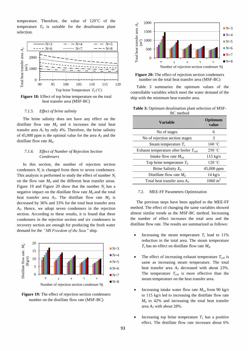
7.1.4. Effect of top brine temperature

The MSF plants usually operate at the top brine

temperatures of 90-120˚C [23]. Therefore, the escalation

of top brine temperature T0 will be at this range. The

distillate flow rate Md is almost constant. Hence, the

selection of the temperature T0 value depends on the trend

of heat transfer areas. The total heat transfer area AT is

inversely proportion with the temperature T0, as shown in

Figure 18. This is a result of increasing the brine heater

heat transfer area Ab by 49% and decreasing in condensers

heat transfer area Ac by 33% with the variation of top brine

5

10

15

20

110 120 130 140 150 160 170 180 190 200

Dis

till

ate

flo

w r

ate

Md

(kg/s

)

Steam temperature TS (˚C)

N=3 N=4 N=5N=6 N=7 N=8

0

1000

2000

3000

4000

110 120 130 140 150 160 170 180 190 200

To

tal

hea

t tr

ansf

er a

rea

AT

(m2)

Steam temperature TS (˚C)

N=3

N=4

N=5

N=6

4

8

12

16

20

250 255 260 265 270 275 280 285 290 295 300

Dis

till

ate

flo

w r

ate

Md

(kg/s

)

Exhaust temperature after boiler Texh (˚C)

N=3N=4N=5N=6N=7

0

500

1000

1500

2000

2500

250 255 260 265 270 275 280 285 290 295 300

To

tal

hea

t tr

ansf

er

area

AT (

m2)

Exhaust temperature after boiler Texh (˚C)

N=

3N=

4

93

temperature. Therefore, the value of 120˚C of the

temperature T0 is suitable for the desalination plant

selection.

Figure 18: Effect of top brine temperature on the total

heat transfer area (MSF-BC)

7.1.5. Effect of brine salinity

The brine salinity does not have any effect on the

distillate flow rate Md and it increases the total heat

transfer area AT by only 4%. Therefore, the brine salinity

of 45,000 ppm is the optimal value for the area AT and the

distillate flow rate Md.

7.1.6. Effect of Number of Rejection Section

Condensers

In this section, the number of rejection section

condensers Nj is changed from three to seven condensers.

This analysis is performed to study the effect of number Nj

on the flow rate Md and the different heat transfer areas.

Figure 19 and Figure 20 show that the number Nj has a

negative impact on the distillate flow rate Md and the total

heat transfer area AT. The distillate flow rate Md is

decreased by 36% and 33% for the total heat transfer area

AT. Hence, we adopt seven condensers in the rejection

section. According to these results, it is found that three

condensers in the rejection section and six condensers in

recovery section are enough for producing the fresh water

demand for the “MS Freedom of the Seas” ship.

Figure 19: The effect of rejection section condensers

number on the distillate flow rate (MSF-BC)

Figure 20: The effect of rejection section condensers

number on the total heat transfer area (MSF-BC)

Table 3 summaries the optimum values of the

controllable variables which meet the water demand of the

ship with the minimum heat transfer area.

Table 3: Optimum desalination plant selection of MSF-

BC method

Variable Optimum

value

No of stages 6

No of rejection section stages 3

Steam temperature Ts 160 ˚C

Exhaust temperature after boiler Texh 250 ˚C

Intake flow rate Mint 115 kg/s

Top brine temperature T0 120 ˚C

Brine Salinity Xb 45,000 ppm

Distillate flow rate Md 14 kg/s

Total heat transfer area AT 1060 m2

7.2. MEE-FF Parameters Optimization

The previous steps have been applied to the MEE-FF

method. The effect of changing the same variables showed

almost similar trends as the MSF-BC method. Increasing

the number of effect increases the total area and the

distillate flow rate. The results are summarized as follows:

Increasing the steam temperature Ts lead to 11%

reduction in the total area. The steam temperature

Ts has no effect on distillate flow rate Md.

The effect of increasing exhaust temperature Texh is

same as increasing steam temperature. The total

heat transfer area AT decreased with about 23%.

The temperature Texh is more effective than the

steam temperature on the heat transfer area.

Increasing intake water flow rate Mint from 90 kg/s

to 115 kg/s led to increasing the distillate flow rate

Md to 42% and increasing the total heat transfer

area AT with about 28%.

Increasing top brine temperature T1 has a positive

effect. The distillate flow rate increases about 6%

0

1000

2000

90 95 100 105 110 115 120

To

tal

hea

t tr

ansf

er a

rea

AT

(m2)

Top brine Temperature T0 (˚C)

N=3 N=4 N=5

N=6 N=7 N=8

0

5

10

15

20

3 4 5 6 7 Dis

till

ate

flo

w r

ate

Md

(Kg/s

)

Number of rejection section condenser Nj

N=3

N=4

N=5

N=6

N=7

N=8

0

500

1000

1500

2000

3 4 5 6 7 To

tal

hea

t tr

ansf

er a

rea

AT

(m2)

Number of rejection section condenser Nj

N=3

N=4

N=5

N=6

N=7

N=8

94

and in the same time, the total area AT decreased

about 79%.

The brine salinity Xb does not have any effect on

distillate flow rate. But the total heat transfer area

decreases with about 8% with increasing the brine

salinity from 45,000 ppm to 80,000 ppm.

Table 4: Optimum desalination plant selection of MEE-

FF method

Variable Optimum

value

No of effects 5

Steam temperature Ts 200 ˚C

Exhaust temperature after boiler Texh 300 ˚C

Intake flow rate Mint 115 kg/s

Top brine temperature T1 90 ˚C

Last effect brine temperature Tn 44 ˚C

Condenser exit temperature Tfn 40 ˚C

Brine Salinity Xb 80,000 ppm

Distillate flow rate Md 14 kg/s

Total heat transfer area AT 1590 m2

7.3. MSF-OT Parameters Optimization

Similar to the previous two methods, this section

studies the effect of the controllable variables on the

distillate flow rate and the heat transfer area. Table 5

shows the input data of MSF-OT program.

Table 5: The input data of MSF-OT program

Variable Input

Value

Range of

change

Co

ntr

oll

ab

le v

ari

ab

les

No of effects NA 3-8

Steam temperature Ts NA 110-200˚C

Exhaust temperature

after boiler Texh 250 ˚C

250 – 300

˚C

Intake flow rate Mint 90 kg/s 90 – 115

kg/s

Top brine temperature

T0 100 ˚C 90-110 ˚C

Feed water Salinity Xf 36,000

ppm NA

Exhaust temperature before

boiler 355 ˚C NA

Sea water temperature before

cooler 24 ˚C NA

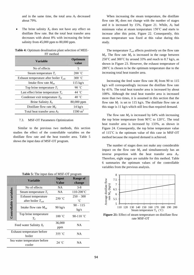
When increasing the steam temperature, the distillate

flow rate Md does not change with the number of stages

and it is increased by 15%, Figure 21. While, AT had

minimum value at steam temperature 150˚C and starts to

increase after this point, Figure 22. Consequently, this

steam temperature was fixed at this value during this

study.

The temperature Texh affects positively on the flow rate

Md. The flow rate Md is increased in the range between

250˚C and 300˚C by around 33% and reach to 8.7 kg/s, as

shown in Figure 23. However, the exhaust temperature of

280˚C is chosen to be the optimum temperature due to the

increasing total heat transfer area.

Increasing the feed water flow rate Mf from 90 to 115

kg/s will correspondingly increase the distillate flow rate

by 41%. The total heat transfer area is increased by about

108%. Although the total heat transfer area is increased

more than two times, it is assumed in this section that the

flow rate Mf is set to 115 kg/s. The distillate flow rate at

this stage is 11 kg/s which still less than required demand.

The flow rate Md is increased by 64% with increasing

the top brine temperature from 90˚C to 120˚C. The total

heat transfer area is increased by 133%, as shown in

Figure 24. Consequently, the top brine temperature value

of 115˚C is the optimum value of this case in MSF-OT

method because the required demand is achieved.

The number of stages does not make any considerable

impact on the flow rate Md and simultaneously has an

inverse proportion with the heat transfer area AT.

Therefore, eight stages are suitable for this method. Table

6 summaries the optimum values of the controllable

variables from the previous analysis.

Figure 21: Effect of steam temperature on distillate flow

rate MSF-OT

5

5.5

6

6.5

7

7.5

8

110 120 130 140 150 160 170 180 190 200

Aver

age

dis

till

ate

flo

w

rate

Md (

kg/s

)

Steam temperature TS (˚C)

95

Figure 22: Effect of steam temperature on total heat

transfer area MSF-OT

Figure 23: Effect of exhaust temperature on distillate flow

rate MSF-OT

Figure 24: Effect of Top brine temperature on total area

MSF-OT

Table 6: Optimum desalination plant selection of MSF-

OT method

Variable Optimum value

No of stages 8

Steam temperature Ts 150 ˚C

Exhaust temperature after boiler Texh 280 ˚C

Intake flow rate Mint 115 kg/s

Top brine temperature T0 115 ˚C

Distillate flow rate Md 14 kg/s

Total heat transfer area AT 1570 m2

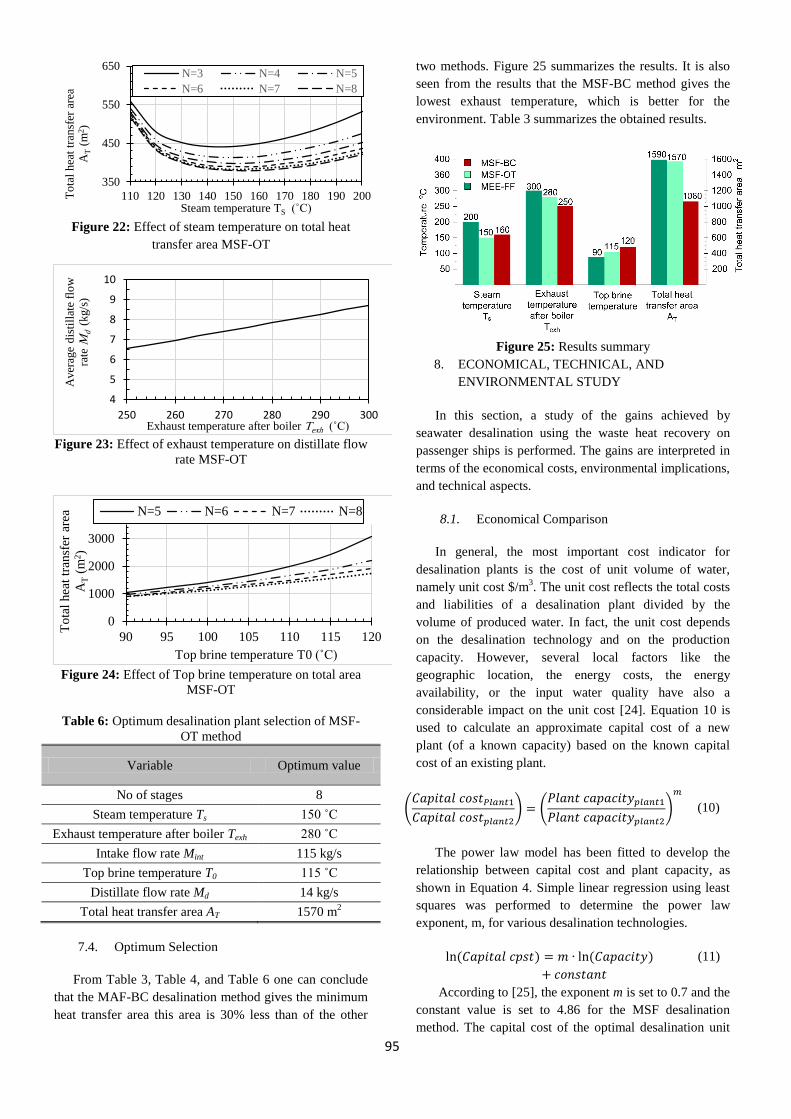
7.4. Optimum Selection

From Table 3, Table 4, and Table 6 one can conclude

that the MAF-BC desalination method gives the minimum

heat transfer area this area is 30% less than of the other

two methods. Figure 25 summarizes the results. It is also

seen from the results that the MSF-BC method gives the

lowest exhaust temperature, which is better for the

environment. Table 3 summarizes the obtained results.

Figure 25: Results summary

8. ECONOMICAL, TECHNICAL, AND

ENVIRONMENTAL STUDY

In this section, a study of the gains achieved by

seawater desalination using the waste heat recovery on

passenger ships is performed. The gains are interpreted in

terms of the economical costs, environmental implications,

and technical aspects.

8.1. Economical Comparison

In general, the most important cost indicator for

desalination plants is the cost of unit volume of water,

namely unit cost $/m3. The unit cost reflects the total costs

and liabilities of a desalination plant divided by the

volume of produced water. In fact, the unit cost depends

on the desalination technology and on the production

capacity. However, several local factors like the

geographic location, the energy costs, the energy

availability, or the input water quality have also a

considerable impact on the unit cost [24]. Equation 10 is

used to calculate an approximate capital cost of a new

plant (of a known capacity) based on the known capital

cost of an existing plant.

(

) (

)

(10)

The power law model has been fitted to develop the

relationship between capital cost and plant capacity, as

shown in Equation 4. Simple linear regression using least

squares was performed to determine the power law

exponent, m, for various desalination technologies.

(11)

According to [25], the exponent m is set to 0.7 and the

constant value is set to 4.86 for the MSF desalination

method. The capital cost of the optimal desalination unit

350

450

550

650

110 120 130 140 150 160 170 180 190 200To

tal

hea

t tr

ansf

er a

rea

AT (

m2)

Steam temperature TS (˚C)

N=3 N=4 N=5

N=6 N=7 N=8

4

5

6

7

8

9

10

250 260 270 280 290 300

Aver

age

dis

till

ate

flo

w

rate

Md (

kg/s

)

Exhaust temperature after boiler Texh (˚C)

0

1000

2000

3000

90 95 100 105 110 115 120

To

tal

hea

t tr

ansf

er a

rea

AT (

m2)

Top brine temperature T0 (˚C)

N=5 N=6 N=7 N=8

96

can be estimated for a capacity of 1211 m3/day. After

computing the capital cost, Equation 12 is used to

determine the Unit Product Cost UPC which is defined as

the sum of the depreciated capital cost and the operating

costs. When unspecified, the plant life has been assumed

to be 20 years with plant availability of 90%.

(

⁄ )

(12)

Equations 10 and 11 produce two extreme values of

the unit's capital cost. Specifically, Equation 3 estimates

the maximum capital cost by $ 5,435,000. In this case, the

unit product cost is equal 1.3 $/m3. About 2.7 $/m

3 can be

saved from the average fresh water price in some ports.

Consequently, the capital cost can be returned after 6

years. Whereas, Equation 4 estimates the minimum capital

cost by $ 1,155,000 where this value can be returned after

one year. Accordingly, the capital return can be achieved

in a range between one and five years due to 0.26 $/ton for

unit product cost. In both cases, the unit's lifetime reaches

20 years. Therefore, a significant profit is gained even

with considering the worst case. Using waste heat energy

to generate fresh water reduces the UPC by 40%. This

value is estimated comparing with the capital cost of MSF

unit in Table 7 [25].

Table 7: Capital cost of various desalination processes

Process Plant capacity

m3/day

Unit-capital cost

$/(m3/day)

MEE 37,850 1860

MSF 37,850 1598

8.2. Environmental Comparison

In case of using dedicated fuels for the desalination

unit, Equation 13 can be used to estimate the fuel

consumption where mf is fuel consumption in kg/s, CV is

the calorific value of the fuel in kj/kg, msteam is the steam

flow rate in kg/s, Cp is the specific heat of the water in

kj/kg and ΔT is the difference temperature between the

output steam and the inlet water. Assuming that the steam

boiler is operated with Heavy Diesel Oil HDO, thus the

fuel consumption is calculated to be 253.5 kg/hr. This fuel

combustion produces an amount of exhaust emission that

can be saved when using the waste heat energy.

Legislation of exhaust emission levels has focused on

carbon monoxide CO, hydrocarbons HC, nitrogen oxides

NOx, and particulate matter PM [26]. According to the

fuel consumption, the amount emission which was

supposed to be emitted is shown in Table 8. Preventing

these emissions obviously has a positive effect on the

environment.

(13)

Table 8: Emission saving due to using WHR

Emission factor Emission saving (kg/hr)

CO2 800

NOx 16

CO 0.7

HC 0.7

Particulates 0.6

SO2 5.3

8.3. Technical Comparison

Eventually, the efficiency of the main diesel engine is

studied before and after applying the proposed system; η1

and η2. Equation 14 states that the efficiency of the engine

is increased by adding the desalination gain power.

Specifically, the thermal efficiency is increased by 2% and

η2 reaches 50.5%.

𝜂

(14)

9. CONCLUSION

In this paper, the fresh water generation on board of a

passenger ship has been studied. Water desalination is

performed using the waste heat energy produced from the

main engine exhaust and the cooling water was proposed.

Three methods have been used for comparison;

Forward Feed Multiple Effect Evaporation MEE-FF, One

Through Multi-Stage Flash MSF-OT, and Brine

Circulation Multi-Stage Flash MSF-BC. Waste heat from

the engine is used for the operation of the desalination

plant. A VB program has been developed to calculate the

desalination plant characteristics. The program was

validated and then it was used to calculate the heat

transfer.

The results showed that the MSF-BC gives the

minimum heat transfer area for the required distillate flow

rate; 30% less than the other two methods. It is found that

the steam temperature Ts, the exhaust temperature Texh, and

the top brine temperature T0 are inversely proportion with

the total heat transfer area AT. Consequently, these

variables have been assigned their maximum values so

that the heat transfer area is minimized. Conversely, the

brine salinity Xb has a direct proportion with the area AT.

Therefore, increasing the salinity normally results in

increasing the area AT.

97

Applying the optimum selection of the proposed salt

water desalination on the case study saved 2.7 $/ m3 as a

minimum comparing to the average cost of fresh water in

ports. This saving can cover the plant capital cost in six

years at most. However, in the best case, the capital cost

was $ 1,115,000 and the unit product cost UPC was 0.26

$/m3.

The plant reduced the emissions by about five

thousand tons of CO2, 100 tons of NOx and 35 tons of SO2

per year.

Finally, the thermal efficiency is of the engine is

increased by 2% (from 48.5% to 50.5%).

So far, the paper proved the efficiency of exhaust gas

and cooling water for deriving the water desalination

units. As an outlook, the work in this paper can be

extended through investigating the efficiency of other

waste heat sources, such as the air cooler and the

lubricating oil. Additionally, the paper focused on thermal

water desalination methods. As an extension is the

application of the reverse osmosis method or hybrid

methods for water desalination on ships. This method is

broadly superior over other methods in the literature

thanks to its simplicity while being adopting.

NOMENCLATURE

Ab Heat transfer area of the brine heater m2

Aj Heat transfer area of the rejection

section stage m

2

Ar Heat transfer area of the recovery

section stage m

2

B Brine flow rate in special effect kg/s

Cair Specific heat of air kj/kg.K

Club Specific heat of lubricating oil kj/kg.K

Cp Specific heat kj/kg.K

Cw Specific heat of water kj/kg.K

D Distillate flow rate in special effect kg/s

FC Fuel consumption kg/s

Hs Specific enthalpy of the steam kj/kg

Hw Specific enthalpy of the water kj/kg

LCV Low calorific value kj/kg

Mcw Cooling water flow rate kg/s

Md Distillate flow rate kg/s

mexh Mass flow rate of exhaust gas kg/s

Mf Feed flow rate kg/s

Mr Recycle stream flow rate Kg/s

MFW Flow rate of fresh water kg/s

mlub Mass flow rate of lubricating oil kg/s

Ms Steam flow rate kg/s

MFW Flow rate of fresh water kg/s

MSW Flow rate of salt water kg/s

mw Mass flow rate of cooling water kg/s

Mw Water flow rate kg/s

Pb Brake power kW

Qcooler Thermal load of the cooler kW

Qexh Heat loss by exhaust kW

Qlub Heat loss by lubricating oil kW

Qrad Heat loss by radiation kW

Qs Supplied fuel energy kW

Qw Heat loss by cooling water kW

T0 Top brine Temperature ˚C

Tb Brine water temperature ˚C

Tcw Cooling water temperature K

Texh(inlet) Exhaust temperature before boiler after

turbocharger K

Texh(outlet) Exhaust temperature after boiler going

to the air ˚C

Tf Feed water temperature ˚C

Tin(FW) Inlet fresh water temperature to the

cooler K

Tin(SW) Inlet salt water temperature to the

cooler K

Tout(FW) Outlet fresh water temperature from the

cooler K

Tout(SW) Outlet salt water temperature from the

cooler K

Xb Brine salinity ppm

Xf Feed water salinity ppm

Xr Recycle stream salinity ppm

REFERENCES

[1] Smalley. R.E, “Future global energy prosperity: the

terawatt challenge,” MRS Bulletin, 30(6), pp.412-

417, 2005.

[2] Alderton. P.M, “Reeds sea transport: operation and

economics” Chapter 2: Types of Ships, pp. 29, A&C

Black, 2004.

[3] Richard. V, “The Design and Construction of a

Modern Cruise Vessel,” Carnival Corporation &

PLC, Retrieved on January 2018.

98

[4] El-Gohary. M. M, and Othman. H.H, “Improving

Green Fresh Water Supply in Passengers Ships

Using Waste Energy Recovery,” Journal of King

Abdulaziz University, 21(2), p.127, 2010.

[5] Mehner, A.C, "Multimedia and Ultra-filtration for

Reverse Osmosis Pretreatment Aboard Naval

Vessels," The University of Arkansas

Undergraduate Research Journal, 11.1, 14, 2010.

[6] Güler. E, Kaya. C, Kabay N, and Arda. M, “Boron

removal from seawater: state-of-the-art review,”

Desalination, 356, pp.85-93, 2015.

[7] Shu. G, Liang. Y, Wei. H, Tian. H, Zhao. J, and

Liu. L, “A review of waste heat recovery on two-

stroke ic engine aboard ships,” Renewable and

Sustainable Energy Reviews, vol. 19, pp. 385–401,

2013.

[8] M. Al-Sahali and H. Ettouney, “Developments in

thermal desalination processes: design, energy, and

costing aspects, ” Desalination, vol. 214, no.1-3, pp.

227–240, 2007.

[9] H. T. El-Dessouky and H. M. Ettouney,

Fundamentals of salt water desalination. Elsevier,

2002.

[10] P. Druetta, P. Aguirre, and S. Mussati,

“Optimization of multieffect evaporation

desalination plants,” Desalination, vol. 311, pp.1–

15, 2013.

[11] N. M. Abdel-Jabbar, H. M. Qiblawey, F. S. Mjalli,

and H. Ettouney, “Simulation of large capacity msf

brine circulation plants,” Desalination, vol. 204, no.

1-3, pp. 501–514, 2007.

[12] Eyringer V, Kӧhler HW, Lauer A, Lemper B.,

Emissions from international shipping: 2. Impact of

future technologies on scenarios until 2050. Journal

of Geophysical Research 2005.

[13] P. Kumar and A. Rehman, “Homogeneous charge

compression ignition (hcci) combustion engine-a

review,” IOSR Journal of Mechanical and Civil

Engineering, vol. 11, no. 6, pp. 47–67, 2014.

[14] D. Dunn-Rankin, "Lean combustion: technology and

control", Academic Press, 2011, ch. Introduction

and Perspectives.

[15] Ship Energy Efficiency Measures: Status and

Guidance, Technical Report, ABS, accessed

January 2018,

https://ww2.eagle.org/content/dam/eagle/advisories-

and-debriefs/ABS_Energy_Efficiency_Advisory.pdf

[16] J. S. Jadhao, D. G. Thombare. "Review on Exhaust

Gas Heat Recovery for I.C. Engine", International

Journal of Engineering and Innovative Technology

(IJEIT), Volume 2, pp 93-100, 2013.

[17] F. Zhou, S. N. Joshi, R. Rhote-Vaney, E. M. Dede,

"A review and future application of Rankine Cycle

to passenger vehicles for waste heat recovery",

Renewable and Sustainable Energy Reviews,

Volume 75, Pages 1008-1021, 2017.

[18] M. Darwish, F. Al-Juwayhel, and H. K.

Abdulraheim, “Multieffect boiling systems from an

energy viewpoint,” Desalination, vol. 194, no. 1, pp.

22 – 39, 2006.

[19] S.-T. Website, “Freedom of the Seas – Cruise Ship,”

http://www.ship-

technology.com/projects/freedomofthesea/

September 2003, [Online; accessed June 2015].

[20] Project guide for Marine Applications, Wärtsilä

Finland oy, Wärtsilä 46,

http://www.lme.ntua.gr:8080/academic-info-

1/prospheromena-mathemata/egkatastaseis-

prooses/PG46.PDF

[21] Royal Caribbean Cruises Ltd. STEWARDSHIP

REPORT, 2012, available at

http://www.royalcaribbean.com/content/en_US/pdf/1

3034530_RCL_2012StwrdshpTwoPgrs_v4.pdf

[22] Dennis P. N, Fire Pump Arrangements at Industrial

Facilities (third edition), Elsevier, 2017.

[23] Khawaji. A. D, Kutubkhanah I. K, and Wie. J.M,

“Advances in seawater desalination technologies,”

Desalination, vol. 221, no. 1-3, pp. 47–69, 2008.

[24] Münk. F, “Ecological and economic analysis of

seawater desalination plants”, university of

Karlsruhe, Diploma thesis, 2008.

[25] Ettouney. H.M, El-Dessouky. H.T, Faibish. R.S,

Gowin. P, "Evaluating the economics of

desalination", Chem. Eng. Prog. 98 (12) 32–40,

2002.

[26] Jadhao. J. S, Thombare D. G. "Review on Exhaust

Gas Heat Recovery for I.C. Engine", International

Journal of Engineering and Innovative Technology

(IJEIT), Volume 2, pp 93-100, 2013.