Warwick Economics Research Papers

ISSN 2059-4283 (online)

ISSN 0083-7350 (print)

Secession with Natural Resources

Amrita Dhillon, Pramila Krishnan, Manasa Patnam and Carlo Perroni

(This paper also appears as CAGE Discussion paper 453)

January 2020 No: 1240

Secession with Natural Resources∗

Amrita Dhillon† Pramila Krishnan‡ Manasa Patnam§ Carlo Perroni¶

December 2019

ABSTRACT

We look at the formation of new Indian states in 2001 to uncover the effects of political secession on

the comparative economic performance of natural resource rich and natural resource poor areas. Re-

source rich constituencies fared comparatively worse within new states that inherited a relatively larger

proportion of natural resources. We argue that these patterns reflect how political reorganisation af-

fected the quality of state governance of natural resources. We describe a model of collusion between

state politicians and resource rent recipients that can account for the relationships we see in the data

between natural resource abundance and post-breakup local outcomes.

KEYWORDS: Natural Resources and Economic Performance, Political Secession, Fiscal Federalism

JEL CLASSIFICATION: D72, H77, O13

SHORT TITLE: Secession with Natural Resources

∗We would like to thank seminar/conference participants at the Political Economy Workshop 2018, Helsinki, Paris Schoolof Economics, Université Libre de Bruxelles, Queen Mary University of London, Kings College, London, University of Cam-bridge, London School of Economics,University of Oxford, European Development Network 2015, Oslo, Delhi School ofEconomics, Indian Statistical Institute, York University, University of Warwick, 3rd InsTED Workshop Indiana University,Econometric Society North American Summer meetings, for their comments. We would also like to thank Denis Cogneau,Stefan Dercon, Douglas Gollin, Eliana La Ferrara, Paolo Santos Monteiro, Kaivan Munshi, Rohini Pande, Andrew Pickering,Debraj Ray, Janne Tukiainen, and two anonymous reviewers for their comments on various versions of this paper. Financialsupport from the LABEX ECODEC (ANR-11-IDEX-0003/Labex Ecodec/ANR-11-LABX-0047) is gratefully acknowledged.

†Dept. of Political Economy, Kings College, London, and CAGE, University of Warwick. Email: amrita.dhillon@kcl.ac.uk.

‡University of Oxford and CEPR, pramila.krishnan@qeh.ox.ac.uk

§CREST-ENSAE, mpatnam1@gmail.com

¶University of Warwick, CAGE and CESIfo, c.perroni@warwick.ac.uk

1 INTRODUCTION

Does political secession yield economic dividends? Evidence on this question is mixed.1 Secessionistmovements are often motivated by economic incentives; and in several cases these incentives relateto the ownership of natural resources (Collier and Hoeffler 2006).2 But some of the effects of politicalsecession come from its effects on governance, effects that may be shaped by the re-allocation of nat-ural resources. Indeed, political secession provides a natural test-bed for investigating whether thewidely-documented adverse influence of natural resources on economic performance (the “curse” ofnatural resources) flows through a political channel.

In this paper, we exploit the formation of three new Indian states in 2001 to examine how post-secession outcomes for local economies vary according to the local distribution of mineral deposits.A key feature of the 2001 Indian secession is that two of the original states contained a significant shareof India’s natural resources, and these were concentrated within specific geographical areas. Figure 1shows the states that were involved: the states that seceded are Jharkhand, Chhattisgarh and Uttarak-hand; the associated rump states are Bihar, Madhya Pradesh and Uttar Pradesh. Figure 2 illustratesthe dramatic shift in control of mineral deposits from the original state to the new states. Table 1 givesa summary of the spatial distribution of natural resource rich (NRR) constituencies pre and post breakup, in Columns 1 and 2. The Bihar-Jharkhand state pair witnessed a large change in the distributionof natural resources upon breakup, with Jharkhand (the new state) obtaining almost all of the min-eral deposits relative to Bihar. The breakup of Madhya Pradesh did mean that a substantial part ofits natural resources accrued to the new state of Chhattisgarh, though Madhya Pradesh remains oneof the states that are richer in natural resources. Finally, the Uttar Pradesh-Uttarakhand state pairsaw a high proportion of mineral deposits go to Uttarakhand. The secession episode thus provides aquasi-natural experimental setting for examining how natural resource endowments are reflected ineconomic outcomes through political reorganisation.

Using a combined spatial discontinuity with difference-in-difference design, we examine the dif-ferential effects of the breakup on economic performance across new (seceding) and old (rump) statesby examining the evolution of economic activity, proxied by luminosity, for 1,124 constituencies in thethree pairs of states, comparing outcomes across the new state borders for 186 assembly constituen-cies (ACs) that are natural resource rich and for 938 ACs that are not, over the period 1992-2010. Thisallows us to study how seceding natural resource rich (NRR) constituencies perform relative to rumpNRR units and how seceding natural resource poor (NRP) constituencies perform relative to rumpNRP units.3 The borders of the assembly constituencies remained the same after secession makingmeaningful comparisons possible. Focusing on longitudinal, within-country comparisons allows usto circumvent some of the problems inherent in cross-country analyses.4

To identify the effect of state breakup on development outcomes, we make use of the geographicdiscontinuity at the boundaries of each pre-breakup state. We additionally exploit the time dimensionof our data as a further source of identification. Essentially, we use the observed changes in outcomes

1Rodríguez-Pose and Stermšek (2015), examine successive secession movements in the former Yugoslavia and find noevidence of an independence premium. Rose (2006), on the other hand, finds no evidence that a larger size is beneficial.Theoretical analyses of the question (e.g. Boffa et al. 2016) have also pointed to a trade-off in decentralisation between thegains from policies that are better matched to local preferences and the potential loss of political accountability that canoccur in smaller jurisdictions.

2E.g., the secession of South Sudan, rich in oil, from the rest of Sudan; or the case of Scotland, where the slogan “It’sScotland’s Oil” was used to promote the cause of independence. Sablik 2015 offers a useful summary.

3An assembly constituency is a state-level electoral unit which, under India’s first-pass-the post electoral system, electsone member of the state legislative body.

4Cust and Poelhekke (2015) discuss these advantages and document other related studies on natural resources in awithin-country context.

1

Figure 1: Reorganisation of states in 2001

The figure shows the breakup of states in 2001. Areas shaded by dots represent newly createdstates; these are the states of Jharkhand, Chhattisgarh and Uttarakhand, which broke away fromBihar, Madhya Pradesh and Uttar Pradesh respectively. The map is representative of the politicalboundaries in 2001 (Administrative Atlas of India, Census of India, 2011).

Figure 2: Distribution of mineral deposits across the reorganised states

The figure shows the distribution of mineral deposits in India, across the states that were reor-ganised in 2002. Mineral deposits are indicated by small circles.

2

Table 1: Endowment of natural resources and growth across states

Proportion of Mines Average Growth Rate(Planning Commission)

Pre-breakup Post-breakup Pre-breakup Post-breakup

State Pair 1:Bihar

0.20.05 4.9 11.4

Jharkhand (New state) 0.65 3.6 6.3

State Pair 2:Madhya Pradesh

0.40.35 4.7 7.6

Chhattisgarh (New State) 0.54 3.1 8.6

State Pair 3:Uttar Pradesh

0.050.02 4 6.8

Uttarakhand (New State) 0.23 4.6 12.3

This table reports the level and change in the proportion of natural resource rich constituencies (i.e, those with miningdeposits) after state reorganisation, as well as the level and change in growth rate (measured by gross state domestic prod-uct), for each state. Figures for the annual growth rate of each state were obtained from the Planning Commission of India’sfigures for state-wise growth.

to difference out fixed, initial differences between units on either side of the border. Our identifyingassumption is, therefore, that the other (initial) underlying discontinuities at the cutoff (for example,due to pre-defined administrative boundaries, like districting, or language differences) are not chang-ing over time, so that the differenced estimates should be unbiased for the local average treatmenteffect.

The results we obtain are striking. Specifically, NRR constituencies perform comparatively worsein the seceding (new) states; economic outcomes for NRP constituencies, on the other hand, are lessaffected by secession. Moreover, we find suggestive evidence of an interaction effect with natural re-source density at state level: NRR ACs in seceding states that inherit a higher proportion of NRR ACsperform worse relative to NRR ACs in the rump states. Our findings are supported at the aggregate levelby figures from the Planning Commission (Table 1, columns 3 and 4), which show that although onaverage new states do better relative to rump states, post break up, we see heterogeneity in outcomes:areas in new states that end up with a much larger abundance of natural resources (Jharkhand) doworse than the rump state, while others perform better. The heterogeneity in outcomes at the localand state level is mirrored in changes in the distribution of natural resources across the newly-formedstates. The heterogeneity in outcomes at the local and state level is mirrored in the distribution ofnatural resources across the newly-formed states. Following breakup, the proportion of ACs that arerich in mineral deposits is 65% in Jharkhand, up from 20% in the original, combined state (Table 1).The corresponding figures for Chhattisgarh and Uttarakhand are respectively 54% (up from 40%), and23% (up from 5%). Thus, not only is the proportion of ACs that are natural resource rich higher forJharkhand than it is for the other two newly-formed states, but Jharkhand is also the new state thatexperiences the largest natural endowment shock.5

5One can find parallel examples at the cross country level elsewhere. Norway seceded from Sweden in 1905. Oil was

3

A natural candidate explanation for this pattern is the change in state-level political institutionsthat followed from secession. And indeed our main finding of the interaction effect between naturalresource abundance created by secession at the state level together with natural resource abundanceat the assembly constituencies (AC) level is strongly suggestive of a channel flowing through a changein the political relationship between states and natural resource rich ACs following secession. In thecase of India, this relationship is shaped by a number of features that are peculiar to the Indian context:(i) property rights to natural resources belong to states rather than to ACs; (ii) power is concentratedat the state level in terms of policing and public goods; (iii) royalty rates on minerals were very low inthe period we consider;6 (iv) there is a well-documented association between rent seeking, criminalactivity and the abundance of natural resources (Vaishnav 2017; Aidt et al. 2011).

Building on this picture, Section 3 models the differential effects of secession on NRR and NRPdistricts as arising from a political bargain struck in NRR constituencies between state-level politi-cians and local rent recipients who control local votes and exchange them for natural resource rents.The greater is the proportion of NRR constituencies in the state, the greater is the state government’scomparative dependence on votes that are delivered by local-level patrons in return for rents, and thelower is political accountability in the state. State secession leads to a change in the proportion ofNRR districts within a state and thus in the comparative importance of votes from NRR constituen-cies. As a result, states that inherit a comparatively large fraction of NRR districts can experience aloss of political accountability following secession, which in turn can lead to more intense rent grab-bing and worse economic outcomes in those areas. This is similar in spirit to the “preference dilutioneffect” described in the literature on lobbying, whereby more centralised decision making can reducethe power of lobbies to influence policies because of increased preference heterogeneity (e.g. de Meloet al. 1993). Our theoretical framework suggests that, when resource endowments are particularlyhigh, they are more likely to lead to perverse outcomes.

The three instances of state breakup that we study translate into only six observed changes in theproportion of NRR districts within the new states by comparison with the original state. Neverthe-less, the patterns that we see in the data are in line with our interpretation that the effects we seecome from the interplay of politics and natural resources. We see differential effects for NRR districtsvarying according to their political leanings. Further corroboration comes from investigating how thecomparative performance of NRP and NRR districts varies with the election cycle: secession changeshow the comparative performance of NRP and NRR districts vary over the cycle. These additionalfindings provides suggestive evidence that this performance gap is shaped by a political channel andthat this channel is affected by political secession. It is also consistent with our interpretation of theeffects of state breakup on the relationship between actors in NRR districts and state-level politicians.As we discuss later, these changes in performance between NRR and NRP areas are hard to reconcilewith alternative explanations.

The remainder of the paper is organised as follows. Section 2 describes the institutional context.Section 3 presents a theoretical model that links political structure with the governance of naturalresources. Section 4 presents the data used for analysis and lays out the identification strategy forestimating the effect of breakup. Sections 5 and 6 report the empirical results. Section 7 concludes.

discovered much later in the 1970s, following which Norway’s growth rate went down from 6.3% to 1.1%, measured over theperiod 1961 to 2016, while Sweden went from 5.7% to 3.2% over the same period (World Bank). More recent cases includethe secession of South Sudan in 2011 with extensive oil resources but facing conflict and negative rates of growth (WorldBank).

6Royalty rates here are not directly comparable to other international rates since they are based on weight rather thanvalue. Shortly after the breakup, in 2004-05, royalty revenues as percentage of total revenue varied from 3.7% in MadhyaPradesh to about 12.5% in natural resource rich Jharkhand.

4

2 THE INSTITUTIONAL CONTEXT

2.1 THE GOVERNANCE OF NATURAL RESOURCES IN INDIA

India has a federal structure, with both national and state assemblies. Members of the twenty-ninestate assemblies are elected in a first past-the-post system. The leader of the majority party or coalitionis responsible for forming the state government. States have executive, fiscal and regulatory powersover a range of subjects that include education, health, infrastructure and law and order.

There is an overlap in authority between the federal government and state governments in thegovernance of natural resource extraction, with both exerting regulatory authority: major mineralssuch as coal and iron ore are regulated by the central government, while minor minerals are entirelyunder state control as laid down in the Mines and Minerals Development and Regulation (MMDR) Actof 1957. Royalty revenues accrue to state budgets, but rates are set by the central government, whichcontrols rates on output as well as any “dead rent” that accrues in the absence of extraction, and alsodecides on environmental clearances for mining. Property rights to land reside in the states, whichare the legal owners of all major mineral resources (except uranium), and claim all royalties. The mainpower of the states derives from the legal authority to grant licenses. However, until recently, therewas no requirement for the royalties and returns from mining to accrue to local areas and the entireproceeds accrue to the state budget.7 There are thus three players involved in royalty on minerals:the Central Government which fixes the royalty rate, mode and frequency of revision; the State Gov-ernment, which collects and appropriates royalty; and the lessee who might be in either the publicor private sector and who pays the royalty according to the rates and terms fixed by the centre to theState.

The split of authority between federal and state agencies with respect to the governance of naturalresources means that the effects of policy decisions at each level are not fully internalised. The roy-alty rates set by the central government are widely seen as being inefficiently low,8 lowering incentivesfor states to allocate extraction rights to efficient operators and to police illegal mining, since royaltiesfrom mining contribute so little to their budgets: royalty revenues in these states, as a percentage of to-tal revenue, averaged to two percent in 2009, while the mining sector’s share of state domestic productis an average of 10-11 percent for Jharkhand and Chhattisgarh over the period 2004-2011 (Chakrabortyand Garg 2015). Low royalty rates also mean that there is little scope for state politicians to translatetheir control rights over natural resources directly into “political rents” for themselves (e.g. by usingroyalty revenues to finance popular public projects or transfers), which in turn means that in order todo so they must use indirect channels to do so (e.g. using allocating natural resource rights to buttresspolitical support). The fact that the authority for policing resides with the state governments while thefederal government decides on which areas can host mining activity produces incentives to evade en-vironmental regulations by operating outside the areas given clearance by the federal government. Allof this has led to conflict between Centre and State about the weak policing and monitoring by stategovernments.9 Given this institutional context, the politics of resource extraction in India takes ona different flavour from that seen in some other federal states. Natural resource rents are controlledby local operators but power resides at the state level- in particular, as mentioned before, the pro-vision of education, health, law and order and rural electrification is firmly under state control. This

7The recent Mines and Minerals (Development and Regulation) Amendment Ordinance, 2015 provides for the creation ofa District Mineral Foundation (DMF) and a National Mineral Exploration Trust (NMET), funded by a percentage of royaltiespaid by lessees and in principle, affording some re-distribution to local communities.

8It is difficult to compare royalty rates with international rates as the latter are mostly ad valorem while in India royaltyrates have been based on weight until recently. A switch to ad valorem rates in 2009 increased revenues on iron ore ten times(Vanden Eynde 2015).

9For an article which discusses the difficulties of Centre/State coordination in policing, see http://bit.ly/1OHFIRM.

5

institutional setting creates the conditions for state-level politicians and local leaders to strike a politi-cal bargain where they trade “subterranean rents” for loyalty and votes.10 This link between state-levelpoliticians and local rent-seekers is incontrovertible: the political scientist Milan Vaishnav documentsthis in detail in his account of the criminality of politicians (Vaishnav 2017). He argues that the risingcost of elections and a shadowy election financing system where parties and candidates under-reportcollections and expenses means that parties prefer “self-financing candidates who do not represent adrain on the finite party coffers but instead contribute ‘rents’ to the party”; and tells of how, in the stateof Jharkhand, the minister in charge of mines (Koda) once disposed of 48 cases in one hour. Indeed,the corruption is so institutionalised that one of the chairmen of Coal India in West Bengal says thatministers would fix monthly payment targets with senior executives of Coal India and this was one ofthe main sources of funding for political parties. According to some reports almost 15-20% of miningrevenues are creamed off every month (see Spectator Magazine, 2009).

At the local level, natural resource rents give rise to widely documented forms of “rent grabbing”,both legal and illegal. Legalised rent grabbing consists of comparatively less efficient but politicallyconnected producers successfully securing resource extraction rights.11 Illegal rent grabbing mainlyconsists of illegal mining. Collusion of local “rent grabbing entrepreneurs” with corrupt state-levelpoliticians is required to sustain either form of rent grabbing.12 Not only do states grant licenses andleases, but the Mines and Minerals Development and Regulation Act 1957 empowers state and centralgovernment officers to enter and inspect any mine at any time. Thus, illegally extracting mineralsfrom these areas requires a degree of endorsement from the state – e.g. the police turning a blind eyeto illegal activity, or favouritism in allocating leases. These rent grabbing activities generate visibleeconomic costs for local economies, ranging from losses in production efficiency and a deteriorationof law and order, to environmental degradation, displacement of local residents, disruption of localinfrastructure — all leading to a crowding out of other economic activities (Baland and Francois 2000,Mehlum et al. 2006).13

The lack of response by state-level governments to such rent-grabbing, despite the fact that theyhave jurisdiction over all mining matters, suggests that there is a bargain being struck, in NRR ACs,between state-level politicians and the local-level political entrepreneurs/patrons, with payments forconcessions made by politicians in relation to natural resource rents – directly, through the allocationof mining rights, and indirectly, through lax controls on how those rights are managed at the locallevel – taking the form of either bribes or increased political support from local constituencies. The

10Indeed, many times the local rent grabbing entrepreneurs become politicians themselves. Asher and Novosad (2016)documents how local mineral rent shocks cause both adverse selection and worse behaviour of politicians in office. Theydescribe how local politicians have direct control over mining operations from which they derive rents. Aidt et al. (2011)shows how stiff competition between parties in India creates an inherent advantage for criminal politicians who can buyvotes or intimidate voters.

11The allocation process itself, however, is often fraught with irregularities: in 2014 the Supreme court ruled that morethan 214 out of 218 coal licences awarded by governments between 1993-2010 were illegal (see BBC News).

12The Shah Commission Report available at http://www.mines.nic.in provides an ongoing saga of the types of ex-cesses that go on in mining areas.

13As a specific example, take the case of coal: “It is a murky subculture that entwines the coal mafia, police, poor villagers,politicians, unions and Coal India officials. Coal workers pay a cut to crime bosses to join their unions, which control accessto jobs, according to law-enforcement and industry officials. Unions demand a ‘goon tax’ from buyers, a fixed fee per tonne,before loading their coal. Buyers must bribe mining companies to get decent-quality coal. The mafia pays off companyofficials, police, politicians and bureaucrats to mine or transport coal illegally.... Corruption is largely local: “The rackets in-clude controlling unions and transport, manipulating coal auctions, extortion, bribery and outright theft of coal. Popularlyknown as the ‘coal mafia’, their tentacles even reach into state-run Coal India, the world’s largest coal miner, its chairmantold Reuters.” (from Reuters Special Report 2013). For other accounts, see http://www.firstpost.com/india/sukma-maoist-attack-malaise-of-naxal-violence-lies-deep-in-illegal-mining-and-political-funding-3408728.html. Also see https://www.spectator.co.uk/2009/09/the-dark-heart-of-indias-economic-rise/ and http://www.scottcarney.com/article/fire-in-the-hole/.

6

latter relies on local rent recipients being able, through either persuasion or coercion of local voters,to deliver a certain volume of votes to whichever candidate or party they choose.

Vote buying is pervasive in India, not only in NRR constituencies (see, e.g., Mitra et al. 2017); and itoften involves handing out gifts or money prior to elections. Nevertheless, there are reasons to expectthat this exchange of votes for favours to happen comparatively more in NRR ACs. This is becausethe state-level government controls the allocation of rights for the exploitation of natural resourcesas well as the enforcement of exploitation rights, but, as discussed earlier, due to the low royalty ratesthat are set by the federal government, the implications of these decisions for state-level revenuesare negligible. State-level politicians thus have control over something that is very valuable to localoperators but involves little economic opportunity cost for state budgets, making it a natural currencyto be spent in a votes-for-favours transaction. Natural-resource poor (NRP) constituencies lack suchcurrency.14

A symptom of the high prevalence of patronage politics in NRR areas is the higher likelihood ofcriminal politicians being elected in mineral rich constituencies. Table 10 shows that, in a sampleof 179 Parliamentary Constituencies (electing federal level MPs), the likelihood of a politician with acriminal record being elected is increasing in the density of mines in that constituency (the coefficientfrom a simple OLS specification is positive and significant at the 5% level). There is also evidence, asshown in Table 10, that vote buying and electoral fraud takes place relatively more in the mineral richareas: using survey responses from the State Election Survey for Jharkhand in 2005, which posed ques-tions to individual voters about perceptions of voting malpractices, and running a logit specificationof perceived voting malpractice within a district against the number of mines within that district, in-cluding district fixed effects and controls for household characteristics, gives a coefficient of 0.28 thatis significant at the 1% level.

2.2 EXOGENEITY OF BORDERS AND THE TIMING OF STATE BREAKUP

Tillin (2013) explores how the breakup of existing states in 2001 came about. She suggests four possi-ble explanations. The first explanation proffered is that of distinct cultural identities in the breakawayareas that have consistently made demands for secession, demands that have progressively gainedprominence since 1947. The basis on which state borders were originally drawn by the State Reorgan-isation Act of 1956 was along linguistic boundaries, but this criterion tended to ignore other ethnicand social boundaries, leading to large tribal populations in some states seeing themselves as ethni-cally distinct and socially neglected. It should be noted, however, that the sharp distinctions alongethnic, social and linguistic lines, in pre-independence have been reduced in time, since migrationand changing demographics have meant more homogeneity particularly along existing sub-regionalor district borders – this point is explored in further detail below when we examine the balancing ofcharacteristics along the border between states (see Table 2). Furthermore, not all these demandswere centred around statehood, but they did involve claims for more local representation and localmanagement of natural resources, both mines and forestries.15 Second, and tied closely to our expla-nation here, Tillin suggests that natural resources were a factor: private interests might have consid-ered it easier to increase resource extraction and intensify production in a smaller jurisdiction, which

14This can be viewed as an extreme case of a more general scenario where vote trading can take place in all constituenciesbut comparatively more so in natural-resource rich ones.

15Tillin (2013) writes “All three of the regions that became states in 2000 saw the emergence of distinctive types of socialmovement in the early 1970s: Chipko, the people’s forestry movement in the Uttarakhand hills; the trade union movementamong miners, the Chhattisgarh Mines Shramik Sangh; and the worker-peasantry movement in Jharkhand led by the Jhark-hand Mukti Morcha (JMM). In all three cases, the issues raised by social movements related primarily to the role of the statein the management of natural resources and the rights of local communities to substantive economic inclusion.”

7

she terms “extension of capitalist interests”.16 The third explanation relates to the changing federalelection context since 1989, when the leading coalition partner, the Bharatiya Janata Party (BJP), firstfavoured granting statehood to boost their popularity in the areas concerned. This is plausible but aswe explain below, a decade later all political parties had reached a consensus on agreeing secession inthese states (Kumar 2010). A final explanation is that the sheer size of the old states made them diffi-cult to govern and that the breakup was attractive to the central government because it meant bettergovernance and more ease of administration – as well as an acknowledgement of local identities.

The list of explanations Tillin (2013) offers for the 2001 breakup flags two potential difficulties inlooking at secession as a true natural experiment. The first relates to how borders between the rumpstate and the breakaway state were determined. This turns out not to be an issue at all because theboundaries of these three new entities have never been in dispute; the areas comprising the new stateswere separate entities before independence from British rule in 1947. For instance, Sharma (1976) dis-cusses a memorandum to the State reorganisation commission in 1955 asking for a separate state ofJharkhand, naming the six districts in Bihar that were eventually separated from Bihar in 2000 (Haz-aribagh, Ranchi, Palamu, Singhbhum, Santhal Parganas and Dhanbad, then Manbhum).17 The Ut-tarakhand Kranti Dal, the regional party formed in 1979 for a separate hill state was determined tounite the eight hill districts in a separate entity. The borders of Uttarakhand were thus determined bythe borders of the eight hill districts that maintained their separate identity on the basis of geographyand cultural distinctiveness; again, these borders were not in dispute. The borders of Chhattisgarhcomprised the eighteen districts where Chhattisgarhi was spoken, and, again, these district bordershave remained the same since independence.18 However, a key challenge for identification is that de-spite the fact that the demarcation was determined in the past, differences across the borders mighthave evolved over time; this is examined further in Table 2 and in Section 5.1.

The second potential difficulty pertains to the timing of the breakup. This timing was determinedby the success of the BJP at the National elections in 1998. The BJP had led a minority government in1996 and had promised to grant statehood to the three new states if it was returned to power. It wasreturned again at the head of a coalition government, but by this time there was a general consensusboth at national and state levels: the other leading party of the Congress supported the change, asdid the state assemblies of the original states before breakup. While there might have been a initialspurt of political activity by the BJP,19 by this time there was little political opposition anywhere tothe demands for statehood. In fact, these demands had grown less vociferous since the early 1990sbecause it was clear that all the major parties were in accord. Part of this unanimity lay in the factthat all three new states lie well within the external boundaries of India and thus posed little threat tothe Union of India, and, equally important, it was clear that there was no political gain to any of theparties in opposing secession. It might be thought that the timing of breakup was related to particularadvantages of the party in power at the Centre; however, given the consensus across parties and the

16Tillin (2013) summarises the views, both pre and post breakup, of Tata Steel, the major investor in Jharkhand, and thatof other industrialists. Tata Steel was happier with a larger state where “politicians were farther away in Bihar” and less likelyto meddle, while others favoured a smaller state where they hoped there would be better law and order and less corruption.However, seven years after secession, things were perhaps even worse in the new state according to them. In brief, therewere clearly mixed views and, far from the urge to expand resource extraction, issues of infrastructure, electricity provisionand law and order loomed large in favouring breakup and evaluating its success.

17It was the case that the borders were formally decided so as to include the districts that consisted of ‘Scheduled Areas’ asdefined in the Constitution, which in turn may have followed the Simon commission of 1930 that defined certain ‘partiallyexcluded areas’. The list of scheduled areas (which are still mentioned as part of the old states) is available at the Ministry ofTribal affairs website here http://tribal.nic.in/Content/StatewiseListofScheduleAreasProfiles.aspx.

18Since 2012 these borders have been redrawn to give nine new districts.

19The BJP and its previous incarnation, the Bharatiya Jan Sangh had always opposed any state breakup until the 1990s,and therefore their agreement was perhaps of note only because of the change; other leading parties had by then allowedthat this was desirable (Mawdsley 2002).

8

fact that state assemblies pre breakup gave their willing assent to the breakup without much dissent,this also turns out to be a non-issue (Kumar 2010).

Finally, given that we concentrate on the role of resources, it should be emphasised that the pricesof minerals played little part in the timing: mineral prices worldwide see a surge only after 2004, fouryears after breakup. In summary, neither the borders of the states nor the timing of breakup can betraced to any particular economic or political advantage for the breakaway states.

2.3 POLITICAL REORGANISATION AND NATURAL RESOURCES

In our empirical analysis, we ask how the relative economic performance of natural resource rich andnatural resource poor areas was affected by secession. Unlike in the Brazilian case studied by Brolloet al. (2013) and by Caselli and Michaels (2013), state breakup in the Indian case could not have pro-duced windfall revenues at the local level that could have directly encouraged direct appropriation ofrents.20 As we have discussed in Section 2, the political bargain between local and state level leadersmight be mediated through bribes or votes. In the Indian case, however, there is no clear reason toexpect bribery incentives to be much affected by secession, given that state breakup does not changethe economic value of mining concessions and that the influence of state politicians on the allocationof rents remains unchanged.

On the other hand, political reorganisation might directly affect incentives to exchange natural re-source rents for local political support. A direct, mechanical effect of secession is a change in the struc-ture of political competition within states: each new state features fewer districts, each accounting fora larger share of the total votes. Then, if control over natural resources is used by state politicians as ameans of securing political support in relevant districts, it is plausible that secession, by changing therelative political weight of NRR constituencies within the new states, would change the calculation ofthe political costs and benefits involved. And indeed, if we look at how secession has affected the com-parative density of natural resource districts across states, we see that the change in some cases hasbeen dramatic: in the case of Bihar, for example, about 65% of all districts in the newly formed state ofJharkhand are natural resource rich, whereas the corresponding proportion pre-breakup was 20% (seeColumn 2, Table 1). In contrast, the state pair 3 (Uttar Pradesh and Uttarakhand) begins with a verysmall endowment of resources and while the split benefited the new state, it should be emphasisedthat a larger share of a small endowment did not benefit it greatly.

We formalise this idea in the next section.

3 POLITICAL SECESSION, NATURAL RESOURCES AND VOTE TRADING

This section presents a stylised theoretical political-economy framework that derives predictions onhow the changes in the concentration of natural resources brought about by secession can translateinto changes in economic outcomes at the local level. The key idea underlying our modelling exerciseis that the adverse effects of the political influence exerted by special interest groups grows strongerthe smaller is the proportion of competing interests that might act to mitigate them.

The specific mechanism we model relates to an electoral accountability channel that operates atthe state level, which arises from a bargaining game in NRR ACs involving vote sellers/patrons at thelocal level and vote buyers or parties at the state level (above and beyond the kind of vote buying

20Anecdotal evidence suggests that most corruption takes place at the stage of the allocation of licences, andthat only a fraction of actual production of minerals is officially reported – see, e.g., https://www.spectator.co.uk/2009/09/the-dark-heart-of-indias-economic-rise/ and http://www.scottcarney.com/article/fire-in-the-hole/.

9

that might occur in any constituency independently of its natural resource endowments). The morevaluable the votes are, the higher will be the concessions (the “price” paid for votes) to local levelintermediaries. These concessions generate negative economic spillovers on the rest of the economy,which erode political support in the electorate, translating into political costs that must be balancedagainst the political gains that directly come from securing votes through patronage politics in theNRR ACs. State secession changes the distribution of NRR and NRP ACs within the newly formedstates and thus alters the political trade-offs involved in vote buying, which in turn affects economicoutcomes in NRR and NRP ACs.

We begin our discussion by presenting a single-state model of vote selling in political equilibriumand then extend it to characterise effects of secession.

3.1 VOTES FOR SALE AND NATURAL RESOURCE DENSITY

Policy Preferences

Consider first a single state with a continuum of mass one of constituencies with populations of iden-tical size. A fraction q ∈ (0, 1) of all constituencies are natural resource rich (NRR) constituencies; theremaining fraction, 1− q , of constituencies are natural resource poor (NRP) and have no natural re-sources.

Each voter in each constituency has an ex-ante ideal point, i , in ideology/policy space [−1/2, 1/2]≡I , with i being uniformly distributed over the support I in each constituency. A voter’s utility is quadrat-ically decreasing in the distance between her ideal policy, i , and the actual policy, i ′: the payoff levelsa voter i obtains from policy i ′ is −(i − i ′)2.

Two parties, L (the incumbent) and R (the challenger), compete in state-level elections. The win-ning party, j ∈ {L , R }, obtains political rents, W , which we assume to be unity without loss of gener-ality. The incumbent party thus aims at maximising expected political rents, P W

j W = P Wj , where P W

j

is the probability of party j winning.

Party L has an exogenously specified platform located at−1/2 in ideology space, while party R hasan exogenously specified platform located at 1/2. The payoff levels a voter i obtains if L and R win theelection are thus respectively U L

i =−(−1/2− i )2, and U Ri =−(1/2− i )2, with the median ideology voter

(i = 0) being indifferent between the two parties. Additionally, there is a stochastic ideology shock, s ,the same in all constituencies and uniformly distributed in [−1/2, 1/2], that shifts the ex-post ideologyof voter i to i + s .21

Voters vote sincerely. For a given ideology shock, s , the shares of votes that are cast respectivelyfor L and R are therefore equal to 1/2 − s and 1/2 + s ; and so, in the absence of any vote trading,the probability of party L party winning coincides with the probability of s being negative and theprobability of party R winning is the probability of s being positive, both of which are equal to 1/2,given the assumed distribution of ideology shocks.22

21This incumbency related shock could be thought of, for example, as being linked to a common but unpredictable as-sessment by voters of the incumbent’s performance while in office. s is a shock in favour of the R party.

22We can assume that if s = 0 each of the two parties wins with equal probability; but since this is a measure zero event, itmakes no difference to the analysis.

10

The Price of Votes

In each NRR constituency, a local leader controls, through intimidation or persuasion, a fraction, v ∈(0, 1/2), of the total votes.23 (In Appendix B we discuss an extension in which there is a continuousdistribution of natural resources across jurisdictions and where the proportion, q , of ACs where votesales take place is endogenised on the basis of an economic calculation linking the value of naturalresource rents with the cost of procuring votes.) The given tranche of votes, v , can only be deliveredto a single party for a price, x . This price is a payment in kind consisting of targeted, natural resourcerelated concessions that translate into rents for the sellers, such as, for example, granting exploitationrights, as well as relaxing restrictions and policing of abuses by those exploiting the natural resourcesillegally. The net economic value of these concessions to the sellers is z x (z > 0). The price can bedelivered to the seller only if the vote buyer wins the election: the seller’s expected payoff if votes aresold to party j for a price x is therefore P W

j z x .

The rent grabbing activities associated with the payment generate a loss of λ x for those voters inthe constituency who do not partake in them, as well as negative spillovers of ρx for voters in otherconstituencies. What we have in mind here are all the negative effects from unregulated mining –such as environmental degradation, underground coal fires that can interfere with other economicactivities, intimidation by criminal gangs that enable rent extraction (Asher and Novosad 2016) – aswell as the economic costs associated with extraction rights being allocated to less efficient operatorsor granted on deposits that should not be exploited on the basis of an economic calculation of socialcosts and benefits.24

Because of these adverse effects, the favours that are delivered in exchange for votes entail a po-litical opportunity cost for the buyer: since the losses associated with the exchange only occur upondelivery of the promised payment if the party that buys the votes is elected, they have the same effectas that of an ideology shift of corresponding magnitude amongst independent voters against the partythat buys the votes. Specifically, suppose that all the votes that are available for sale in all constituen-cies are purchased by a single party, and that the transaction can be observed by voters;25 independentvoters in NRR constituencies would then anticipate an overall loss (λ+ρq ) x from a win by that party,whereas the prospective loss for for voters in NRP constituencies is ρq x .

The buyer, in its calculation, must balance off this loss of political support amongst independentvoters against the electoral advantage of being able to secure a fraction of the votes directly throughvote buying. In NRR constituencies the political cost arising from the promised delivery of the pay-ment is offset by the political gain from buying votes, but in NRP constituencies it is not. Becauseof this asymmetry, an increase in the proportion, q , of NRR constituencies makes vote buying moreattractive, raising the equilibrium price of the votes that are available for sale:

Proposition 1: Consider the a single (collusive) vote seller making a take-it-or-leave-it offer to a single

buyer. The unique payoff maximising price for the seller is x =v

λ (1− v ) +ρ (1−q v ). This price is de-

creasing in ρ and increasing in q , and its elasticity with respect to changes in q is also increasing in q .The corresponding equilibrium values of P W

L are also decreasing in ρ and increasing in q .

23For accounts of the extent to which local leaders exert control upon the votes of local populations, see Rao (1983) andSingh and Harriss-White (2019).

24For example, blasting and drilling around the coal mines lead to water aquifers drying up, air and noise pollution leadingto a shortage of clean drinking water and water borne diseases to increase, loss of forest reserves, loss of agricultural land,disruption of economic activity by Maoist insurgents (Chauhan 2010). These effects would not be limited only to miningregions but would spill over to neighbouring NRP ACs – particularly SO2 emissions, pollution of surface water, spilloversfrom criminal activities and insurgency.

25Indian voters are well aware of which parties or politicians receive the support of NR lobbies (Arjjumend 2004).

11

(The proof is in Appendix B.)

Allowing for multiple buyers or sellers does not change conclusions. The results of Proposition1 carry over to a scenario where neither party has all the bargaining power – e.g., under sequentialbargaining with alternating offers (Rubinstein 1982). Both extensions are discussed in Appendix B.

An increase in the density of natural resources, via a political channel, raises x and thus lowerseconomic performance (welfare) in NRR constituencies (for individuals other than the vote sellers),as well as in NRP constituencies, albeit to a lesser extent. The intuition for this result is as follows.In its choice of x , the incumbent party balances the net gain in vote share from raising x in NRRconstituencies with the net loss in NRP constituencies. As the proportion of NRR constituencies (q )becomes larger – and the proportion of NRP constituencies (1−q ) becomes smaller – the positive votegains from vote buying in NRR constituencies increasingly come to dominate the political “dilution”effect that comes from the purely negative political spillovers in NRP constituencies, and so the netpolitical value of vote buying (and hence the maximum price that can be paid for it) increases.

Proposition 1 also implies that the dilution effect fades progressively faster as q increases: intu-itively, the strength of the diluting influence of NRP constituencies is related to the ratio (1− q )/q ,which decreases with q at at an increasing rate (in absolute value). As a result, the adverse effects ofan increase in the proportion of NRR ACs become progressively larger.

3.2 EFFECTS OF STATE BREAKUP

State breakup can produce a change in the proportion of NRR districts within the new states relative tothe original state. The predictions we have derived in the previous section for a single-state scenariothus translate into predictions on the effects of state breakup on governance outcomes – predictionsthat in principle could be tested empirically in longitudinal evidence on pre- and post-secession out-comes.

Consider a unified state, U , with a unit mass of constituencies, a fraction qU of which are NRR con-stituencies; and suppose that the unified state breaks up into two new equally-sized states, A and B ,each with a mass of 1/2 constituencies and proportions qA and qB of NRR constituencies. Then, focus-ing only on the component of utility that depends on x , welfare for a citizen i in a NRP constituencyin state H ∈ {A, B } can be expressed as

U N R PH =−ρ

qH xH +γq−H x−H

2, H ∈ {A, B }; (1)

while that for the citizen in a NRR constituency is

U N R RH =U N R P

H −λxH , H ∈ {A, B }, (2)

where γ< 1 reflects a reduction in transboundary spillovers coming from the separation of state insti-tutions, and (qA +qB )/2= qU .26

Votes in H only affect xH , and so only the terms that involve xH in (1) and (2) are relevant forcharacterising voting choices in H . In turn, xH depends on qH via the equilibrium condition describedin Proposition 1.

We are then in a position to draw conclusions concerning how secession affects economic perfor-mance via the political channel described in 3.1 (i.e. abstracting for the time being from effects directlyassociated with the redistribution of revenues from natural resources):

26We abstract from any idiosyncratic component of utility stemming both from ideology and from other factors that donot depend on xH .

12

Proposition 2: The ratio U N R PA /U N R P

B and U N R RA /U N R P

A are both increasing in qA/qB . As levels ofutility are normalised in the model to be negative, this means that, following secession:

(i) comparing across states, U N R PA is smaller, relative to U N R P

B , the larger is qA relative to qB ;

(ii) within state A, U N R RA is smaller, relative to U N R R

A , the larger is qA relative to qB .

(The proof is in Appendix B.)

This result follows immediately from our analysis of a single-state scenario. A higher proportion ofnatural resource rich districts within a state worsens the quality of governance, and hence economicperformance, in that state. To the extent that spillover effects across states are weaker than thosewithin states, this implies that, when we consider only those effects of natural resources that flowthrough a governance channel, an unequal allocation of NRR districts following secession penalisesthe state that receives the larger share (prediction 2.(i)); and, more specifically, worsens the compara-tive economic performance of NRR areas relative to that of NRP areas (prediction 2.(ii)). As explainedin the introduction, this is similar to a “preference dilution effect” whereby more centralised decisionmaking reduces the power of lobbies to influence policies. In our particular context, secession hassimilar effects to decentralisation where the power of local rent seeking lobbies in NRR ACs increasesrelative to other interest groups when their relative weight increases.

Proposition 2 isolates those effects of secession that flow through the political channel we havedescribed in 2.1, but secession also produces effects that flow directly through the redistribution ofnatural resource revenues. These effect relate to the change in the natural resource tax base base,(qA − qU )r , where r is total income from natural resources in a representative NRR ACs. An increasein q relative to its pre-secession level produces an increase in the tax base (relative to the size of thenew state), which may either translate into more provision of public goods, either state-wide or at theNRR AC level, or, alternatively, into a lower level of taxation holding the level of public goods provisionconstant, leaving more disposable income within NRR ACs.27 Through this effect, an increase in qcan potentially raise economic performance in the new state, and, more specifically, in NRR ACs; andindeed, as discussed, the reallocation of revenues from natural resources is often a primary motivationfor secession demands.

Proposition 1 says that the effects of an increase in q on x increase with q – as the diluting influenceof the remaining fraction, 1− q , of NRP ACs becomes progressively smaller, the elasticity of x withrespect to changes in 1 becomes larges, (i.e. the cost associated with a higher q is convex in q ). Andso, if the post-secession level of q A is large enough, the adverse governance effects of an increase inq A , as described by Proposition 2, are more likely to dominate any other positive effects (such as thoseeffects that are associated with an increase in the tax base, which is linear in q ), leading to NRR ACsdoing comparatively worse than NRP ACs in state A post secession (result 2.(ii)):

Proposition 3: Political secession is more likely to lead to a deterioration in the comparative economicperformance of NRR ACs relative to that of NRP ACs of the breakaway state the larger is the density ofnatural resources in the breakaway state post secession.

The predictions of the theory in relation to the effects of political secession can be summarised asfollows:

27There may be other effects of the breakup on economic performance that are independent of the endowment of naturalresources – effects that our analysis abstracts from. For example, the smaller size of each state post breakup might makeadministration easier, as well as allowing a better representation of the electorate.

13

• an increase in the proportion of NRR (q ) in a breakaway state following secession will weaken thediluting effect that NRP areas exert on the political influence of natural resource rents recipientsin NRR areas and lower the quality of governance and thus economic performance;

• this effect is more likely to dominate other positive effects associated with increased ownershipof natural resources in the breakaway state (and result in a comparative worsening in the eco-nomic performance of NRR ACs relative to that of NRP ACs) the larger is q in the breakaway statepost secession.

4 DATA

To study how differences in local outcomes (assembly constituency level) relate to natural resourceswe rely on two main data sources.

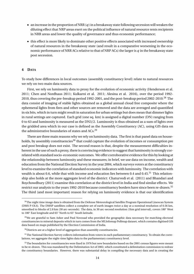
First, we rely on luminosity data to proxy for the evolution of economic activity (Henderson et al.2011; Chen and Nordhaus 2011; Kulkarni et al. 2011; Alesina et al. 2016), over the period 1992-2010, thus covering the pre-breakup period 1992-2001, and the post-breakup period 2002-2010.28 Thedata consist of imaging of stable lights obtained as a global annual cloud free composite where theephemeral lights from fires and other sources are removed and the data are averaged and quantifiedin six bits, which in turn might result in saturation for urban settings but does mean that dimmer lightsin rural settings are captured. Each grid (one sq. km) is assigned a digital number (DN) ranging from0 to 63 and luminosity is measured as the DN3/2. Luminosity is thus obtained as a sum of lights overthe gridded area which in our case is defined as the Assembly Constituency (AC), using GIS data onthe administrative boundaries of states and ACs.29

There are three main reasons why we rely on luminosity data. The first is that panel data on house-holds, by assembly constituencies30 that could capture the evolution of incomes or consumption preand post breakup does not exist. The second reason is that, despite the measurement difficulties in-herent in the use of such a proxy, there is convincing evidence to suggest that luminosity is strongly cor-related with standard socio-economic outcomes. We offer corroborative evidence for this by looking atthe relationship between luminosity and these measures; in brief, we use data on income, wealth andeducation from the National Election Survey in the year 2004, which surveys voters at the constituencylevel to examine the correlation of standard economic indicators with luminosity. The correlation withwealth is about 0.6, while that with income and education lies between 0.4 and 0.45.31 This relation-ship also holds at the more aggregate level of the district: Chaturvedi et al. (2011) and Bhandari andRoychowdhury (2011) examine this correlation at the district level in India and find similar effects. Werestrict our analysis to the years 1992-2010 because constituency borders have since been re-drawn.32

The third (and most important) reason for relying on luminosity evidence is that our identification

28The night time image data is obtained from the Defense Meteorological Satellite Program Operational Linescan System(DMS P-OLS). The DMSP satellites collect a complete set of earth images twice a day at a nominal resolution of 0.56 km,smoothed to blocks of 2.8 km (30 arc-seconds). The data, in 30 arc-second resolution (1km grid interval), covers 180◦ Westto 180◦ East longitude and 65◦ North to 65◦ South latitude.

29We are grateful to Sam Asher and Paul Novosad who provided the geographic data necessary for matching electoralconstituencies to mineral deposits which in turn comes from the MLInfomap Pollmap dataset, which contains digitised GISdata based on maps published by the Election Commission of India.

30Districts are at a higher level of aggregation than assembly constituencies.

31The National Election Survey collects information from voters in each parliamentary constituency. To obtain the corre-lations, we aggregate the night-time lights data to the parliamentary constituency level.

32The boundaries for constituencies were fixed in 1976 but new boundaries based on the 2001 census figures were meantto be re-drawn. This was mandated by the Delimitation Act of 2002, which constituted a delimitation commission to redrawthe constituency boundaries. However, there was substantial delay in compiling the necessary data and in creating the

14

strategy focuses on changes in outcomes rather than levels. This means that sources of persistent het-erogeneity across ACs in the relationship between luminosity levels and levels of economic activityare not a concern.

To corroborate our measure of night-time lights, we use data from two waves (1992 and 2004) ofthe India Human Development Survey (IHDS). Finally we also use data from the Census of India, stateelection results (obtained from the Election Commission of India) and state electricity prices (obtainedfrom India Stat) to support our identification strategy, described in the next subsection. Appendix Aprovides further details on these data sources.

The second type of data we use are data on the location, type and size of mineral deposits from theMineral Atlas of India (Geological Survey of India, 2001).33 Minerals are grouped into nine categories,and each commodity is classified by size, which is proportional to the estimated reserve of the deposit.The definition of the size categories for each commodity is in terms of metric tons of the substancesof reserves contained before exploitation or actual output. This provides comprehensive informationabout the mineral resource potential of the deposits.34

We use data on location specific mineral resources or deposits, rather than their value, to avoid is-sues of endogeneity: the price of minerals found in these deposits is time-varying and can be affectedby various unobservables such as election cycles, and other demand and supply factors that tend tobe correlated with growth and inequality. Also, our empirical strategy relies on a spatial discontinu-ity design with comparisons across borders over time where deposit types are similar, obviating theneed to examine values. Furthermore, as will be clear below, our fixed-effects strategy allows us tonet out the fixed location specific unobservables associated with deposit coverage. Further, the loca-tion of deposits is strictly of geological origin, and the location was mapped before 1975 and hence itsexploration cannot be thought to be controlled by subsequent political and economic incentives orinstitutional factors.

4.1 IDENTIFICATION AND ESTIMATION

In what follows, we conventionally define ACs in the states that have broken away as those that are“treated” by the act of secession. Admittedly, the rump state is also a new creation and is thus affectedby the treatment; so, what we are actually picking up are the differential effects of the treatment (se-cession) between old and new states.35 As evidenced by Table 1, the new states are those that inherita disproportionate number of NRR ACs, and so ”treatment” for an AC can also be interpreted as be-longing to a state that experiences an increase in the proportion of its NRR districts (corresponding toan increase in q in our theoretical model). To identify the effect of state breakup on development out-comes, we make use of the geographic discontinuity at the boundaries of each pre-breakup state andemploy a Regression Discontinuity Design (RDD). For each geographic location, assignment to “treat-ment” (or new state) was determined entirely on the basis of their location. This key feature of thestate breakup allows us to employ a sharp regression discontinuity design to estimate the causal effectof secession on growth. Such a discontinuity is clearly supported by Figure 3, where local polyno-

new boundaries, the first election with redrawn boundaries was only held in Karnataka in 2008. Consequently, the periodbetween 1976 and 2009 in these states had fixed constituencies boundaries allowing for the comparison of luminosity acrosstime.

33Resources are usually classified as point resources and dispersed resources, the former being the most easily appropri-ated. Our focus in this paper is on minerals that are point source resources.

34We are particularly grateful to Sam Asher for sharing his data obtained from the Mineral Atlas and to officials at theGeological Survey of India, Bangalore for clarifying the observations on size.

35This convention is also consistent with the idea that the rump state retains the old institutions and government struc-tures while the new state must create new structures, even if similar to those in the rump state. Rump states saw no reor-ganisation apart from the loss of territories and thus a lower population and smaller administration.

15

mial estimates of the growth in light intensity – the variable relevant for our difference-in-differencecombined with RDD identification strategy described below – around the distance to the thresholdbefore and after breakup are displayed. Figure 4 assesses the validity of the identifying assumptionwith the McCrory (2008) test for breaks in the density of the forcing variable at the treatment borderwith negative distances to state border for old states and positive distances for new states. The figureclearly shows that the density does not change discontinuously across the border, suggesting that forthe window around the coverage border there seems to be no manipulation. This is to be expectedgiven the firm exogeneity of the borders, but it is reassuring all the same.

We define a variable, Di , as constituency i ’s distance to the geographic border d that splits eachof these geographic location between old and new states. We then define an indicator for each AC forbelonging to the new state as

Ti =1[Di≥d ]. (3)

The discontinuity in the treatment status implies that local average treatment effects (LATE) are non-parametrically identified (Hahn et al. 2001). Effectively we compare outcomes for constituencies oneither side of the geographic border that determined treatment assignment or being in a New State.Formally, the average causal effect of the treatment at the discontinuity point is then given by (Imbensand Lemieux 2008):

τa = limg→d+

E[Yi t |Di = g ]− limg→d−

E[Yi t |Di = g ] =E[Yi t (1)−Yi t (0) |Di = d ], (4)

where Yi t is the satellite light density of constituency i in year t .

An important feature to note in the above-mentioned design is that the discontinuity is geographi-cal, i.e., it separates individuals (ACs) in different locations based on a threshold along a given distance-based border. Using (4) to estimate the causal effect would ignore the two-dimensional spatial aspectof the discontinuity. This is because the border line can be viewed as a collection of many points overthe entire distance spanned by the border. For example, an individual located north-west of the bor-der is not directly comparable to an individual located south-east of the border. For the comparisonto be accurate, each “treatment” individual must be matched with “control” individuals who are inclose proximity to their own location and to the border line. We address this issue as follows. We di-vide the border for each state into a collection of points defined by latitude and longitude spaced atequal intervals of 15 kilometers. We then measure the distance of each AC to the border and includepolynomials of distance and its interactions with the treatment variable. We then condition on thepost-breakup interacted, border segment fixed effects in all the specifications, so that only ACs withinclose proximity of each other are compared.36

The local average treatment effect can be estimated using local linear regression by including poly-nomials of distance to the border (controlling for border segment fixed effects) to a sample of unitscontained within a bandwidth distance h on either side of the discontinuity.

We additionally exploit the time dimension of our data as a further source of identification. Theidentification strategy described so far exploits differences across nearby bordering units, post statebreakup to investigate the effect of breakup. Even then, it is possible that there is an underlying admin-istrative discontinuity at the border cutoff in the absence of breakup, since the geographical borderwas laid around existing districts. To address this issue, we use the observed jump in outcomes to dif-ference out such fixed, initial differences between units on either side of the border. Our identifyingassumption is, therefore, that the jumps at the cutoff are not changing over time in the absence of

36See Black (1999), who first discussed the use of the border segments in a regression discontinuity framework. For arecent application, see Dell (2010), who extends the approach to incorporate a semi-parametric regression discontinuitydesign.

16

Figure 3: Growth in light intensity after secession

The figure plots the local polynomial estimates of the growth in light intensity, definedas the difference in average light intensity post (2001-2009) and pre (1992-2000) thesecession, around the threshold distance.

Figure 4: RD validity: density smoothness test for distance to state border

The figure plots test for density smoothness proposed by (McCrary 2008). The dis-tances are normalised, such that positive values indicate distances for new states whilenegative values indicate distances for old states.

17

treatment, so that the differenced local Wald estimators will be unbiased for the local average treat-ment effect.

Our overall identification strategy effectively combines the RDD design with a difference-in-differenceapproach. A key identifying assumption of this empirical strategy is that of conditional commontrends before the secession for areas close to the border. We discuss this assumption further and ex-amine its empirical validity in Section 5.4.

With this in mind, the specification we estimate is

Yi t =αi +βt +γTi ×Postt +δ′Vi t +ςs ×Postt + εi t , (5)

where Yi t is the satellite light density of AC i in year t . αi is the fixed effect for each AC. The variableof interest, the new state effect, is denoted by the interaction of Ti , being located in the new state, andPostt =1[t≥2001]. We control for border segment fixed effects, ςs (interacted with Postt to account forthe panel dimension). The terms αi and βt represent constituency and time fixed effects respectively.The Vi t ’s are defined as

Vi t =

�

1[Di<d ]×Postt × (Di −d )1[Di≥d ]×Postt × (Di −d )

�

. (6)

The regressors Vi t are introduced to avoid asymptotic bias in the estimates (Hahn et al. 2001, Imbensand Lemieux 2008). Standard tests remain asymptotically valid when these regressors are added.

A panel fixed-effects estimator around the distance thresholds, h , is equivalent to using a uniformkernel for local linear regression, as suggested by Hahn et al. (2001). We consider several bandwidths,based on the optimal bandwidth calculations of Imbens and Kalyanaraman (2011), and for each wederive OLS-FE estimates using observations lying within the respective distance thresholds.

5 ESTIMATION RESULTS

5.1 BORDER EXOGENEITY AND BALANCING TESTS OF COVARIATES

Our spatial discontinuity design compares ACs across borders, with the basic notion that differences

in patterns of local activity, controlling for time-invariant characteristics before breakup can only be

attributed to the secession rather than differences due to other factors. This in turn depends on the

variation in observable attributes including human and physical geography. The demarcation of the

borders here are historically determined, based on ethno-linguistic differences as they were present

in 1947 at independence, or even earlier. If the historical demarcation implies a different settlement

by these groups today, this in turn might pose a threat to identification.

To examine this we check how observed characteristics vary at different levels of aggregation across

borders, paying particular attention to differences within a narrow radius of the new-state border (see

for e.g., Lowes et al. 2017, for a discussion of a similar strategy). In Table 2, we present balancing tests

for each covariate based on both the full and restricted sample of observations. In our restricted sam-

ple, we limit the set of observations to a distance bandwidth of 200 km around the border (at the AC

level) or directly bordering districts (at the district level). For each type of sample-set we first report

the mean (in parenthesis the standard deviation) of the entire sample and then report the mean dif-

ferences between rump and new states (in parenthesis the standard error of the differences). In the

first panel, we report the differences across AC-specific characteristics, our preferred unit of analysis.

For our main outcome variable, luminosity, we find that while there were significant differences be-

tween the rump and new state before breakup in the full sample, these differences disappear in the

restricted border sample. A similar pattern holds for the number of conflict occurrences. One variable

18

that remains significant even within our restricted border-sample is the constituencies’ mineral en-

dowments. However, we should expect a-priori such a difference and is the basis of our empirical ex-

ploration that links secession to natural resources distribution. However to account for this difference,

we use constituency fixed effects in our empirical strategy to difference out this time-invariant en-

dowment. Additionally, we check the robustness of our results to differential mineral-specific trends

(for e.g., price effects) and show that our results are not affected by this (in Section 5.3). In sum, our

difference-in-difference strategy does control for fixed pre-breakup differences such as mineral en-

dowment – this is less of a threat to identification than time varying differences reported below.

We also focus on district-level characteristics, and use information from the 2001 socio-economic

census to examine two key characteristics, education and caste composition, that could influence

outcomes. The table shows that for both variables, proportion of literates and proportion of back-

ward caste population, the restricted sample differences between the rump and new state are small,

and much lower compared to the full sample. We do find a small statistical difference in the percent-

age of backward caste population in the restricted sample but show later (in Section 5.3) that the trend

differential is not statistically significant, as required by the common trends assumption of our iden-

tification strategy. We also find no significant difference in the average size of districts across borders,

within the restricted sample. Another possible source of bias is the extent of fractionalisation based

on linguistic differences across borders. Since the breakup was partly motivated by linguistic differ-

ences, it is possible that the areas in the new states were linguistically more fragmented which could

indirectly impact economic outcomes (Alesina et al. 2003). Using information from two rounds of

the Language Atlas of India, we construct measures of linguistic fractionalisation based on Alesina

et al. (2003), and find that the measure is stable and statistically not different between the rump and

new-state bordering districts.

Next, we use information from the IHDS on income, consumption expenditures, measures of

health (proxied by infant mortality) and public goods access (proxied by the distance to piped water),

to see if these variables were different across border areas before breakup (year 1992 of the IHDS sur-

vey). We conclude that they are not, in the restricted border sample. Finally, we examine firm-specific

covariate differentials, combining data on all establishments from the Economic Census (year 1998)

and supplementing it with information on a sample of firms from the Annual Survey of Industries

(year 2001). Significant differences in employment or wage patterns could represent a threat to our

identification as they could shift the distribution of economic outcomes post-secession. However, as

Table 2 shows, we find that while significant differences exist in the full-sample, the restricted border

sample means match well across all covariates, leaving small and statistically insignificant difference

across borders.

5.2 RDD ESTIMATES

We begin with the overall effect of state breakup on the difference in luminosity in Table 3, before mov-

ing on to our main results on how they vary with state-level natural resource abundance. The variable

Post captures the trend across states post breakup while ‘Post×New State’ captures the difference be-

tween the new and rump states on average, post breakup. The first two columns of the table report

the OLS estimate of breakup for the entire sample of ACs across all six states, reporting effects with-

out and with border segment fixed effects. The naive OLS specifications suggest that while all states

experience trend increase in luminosity, on average new states did better than the rump states.

There may be other unobservables linked to state borders that might bias the OLS estimates. To

address these concerns, we present RDD estimates in columns 3-5 of the table. We choose three band-

widths with distance thresholds of 150km, 200km and 250km throughout our analysis. We choose

19

Table 2: Descriptive Statistics and Balancing Tests

FULL SAMPLE RESTRICTED BORDER SAMPLE

Mean (SD) Rump vs. NewState BaselineDifference

Mean (SD) Rump vs NewState BaselineDifference

Assembly Constituency Covariates; N=10,116(F), 5985(R)

Log Luminosity 6.589 0.730*** 6.164 −0.00493(2.260) (0.0616) (2.582) (0.0805)

Mineral Quality 0.006 −0.0210*** 0.009 −0.0214***(0.0503) (0.00120) (0.0641) (0.00173)

# Conflict Occurrences 0.353 −0.00924*** 0.417 0.00427(2.613) (0.00282) (2.091) (0.00391)

District Covariates; N=199(F), 38(R)

Linguistic Fractionalisation (1992) 0.208 −0.153*** 0.278 −0.0266(0.186) (0.0291) (0.185) (0.0607)

Linguistic Fractionalisation (2002) 0.209 −0.143*** 0.278 −0.0257(0.195) (0.0310) (0.181) (0.0595)

Area (in KMs) 4590.8 −1463.8*** 4776.0 −365.0(2844.4) (464.4) (2914.4) (956.7)

Proportion Literate 0.465 −0.0510*** 0.438 −0.0451(0.103) (0.0171) (0.102) (0.0328)

Proportion SC/ST 0.277 −0.120*** 0.287 −0.0768*(0.146) (0.0230) (0.143) (0.0451)

Household Covariates; N=2454(F), 520(R)

Log Income 8.745 0.0752** 8.685 0.0244(1.180) (0.0338) (1.082) (0.0621)

Log Food Expenditure 5.666 0.003 5.479 0.033(1.198) (0.0183) (0.493) (1.110)

Distance to Piped Water 9.293 −0.778 6.230 0.775(36.82) (2.059) (29.61) (3.115)

Caste Category 2.556 −0.331*** 2.711 0.164(1.028) (0.0463) (1.146) (0.106)

Firm Covariates; N=6,610,225(F), 1,172,856(R)

# Workers 3.580 −0.625*** 3.574 −0.036(49.213) (0.050) (35.624) (0.068)

% Mining Workers in District 0.888 −1.440*** 1.173 0.280(3.703) (0.610) (3.187) (1.047)

Wages & Salaries Paid‡ 14.28 −15.96*** 10.35 −0.632(172.85) (5.533) (92.85) (5.815)

Consumption of Electricity & Water‡ 20.46 −20.42*** 17.01 16.14(214.9) (6.972) (189.9) (12.15)

The table reports results the mean (in parentheses standard deviation) of geographic, household and firm-level variables and their differences between the rump and old states (in parenthesis the standard error of thedifferences). The sample size for each panel are indicated for both the full sample (F) and restricted bordersample (R). ‡ variables are obtained from the Annual Survey of Industries for the year 2000; the sample sizefor these variables is 5057(F) and 999(R). * indicates significance at 10%; ** at 5%; *** at 1%.

20

these thresholds based on our calculations of the optimal bandwidth (Imbens and Kalyanaraman

2011). Our calculations indicate an average optimal bandwidth of 181.36, across all post-breakup

years. Its year-wise value ranges from 165.04 to 204.32, all values lying well within our chosen band-

width span. The RDD estimates suggest the same pattern of results as the OLS, albeit with a much

smaller positive growth effect for the new state. We find that the new states did better than the rump

states, with a differential in luminosity of 35 percent. Note that the last four columns include border-

segment fixed effects allowing the absorption of any unobserved characteristics that are similar across

shared boundary segments (Black 1999).

The above results hide a considerable degree of heterogeneity across ACs within states. Table 4

shows how local post-breakup effects are shaped by local natural resources. While ACs with a high

concentration of deposits do relatively better across all states, they do worse in comparative terms if

they are in the new states, post breakup. So, while natural resource rich ACs do better than natural

resource poor ACs on average following the break-up, and ACs in new states do better on average

relative to ACs in rump states, natural resource rich ACs do comparatively worse in the new states.

Since the identification strategy we employ isolates the effects of state breakup from the effects of other

possible concurrent factors, these results show that these effects come from an interaction between

state breakup and natural resource endowments at the AC level, with the interaction effect operating

differently in the new states and the rump states.

Analogous patterns are in evidence if we focus on outcomes other than luminosity for a sample

of households located in districts that lie along the border of the old and new state (Table 5).37 On

the whole, we find positive effects of breakup on all household level outcomes but negative effects for

those ACs in mineral rich ACs of new states, mirroring the results in Table 3: households in mineral-

rich ACs of new states saw a decrease in income and food expenditure and, at the same time, an in-

crease in infant mortality relative to their peer mineral-poor ACs and other ACs in the rump states.

If we next look at how breakup affects outcomes separately in each of the new states, employing

a specification where the single New State indicator is replaced by state-specific indicators (Table 6),

a mixed picture takes shape. Effects in one new state (Uttarakhand) are better than that its rump, Ut-

tar Pradesh, but worse for Jharkhand and Chhattisgarh relative to their rumps, and these differences

are strongly significant. These stark differences are matched by an equally stark variation in how the

natural resource rich (NRR) regions were distributed between the rump state and the new state post

break up (Table 1, column 2). Note that the OLS coefficient estimates for Jharkhand are negative when

border-segment fixed effects are included in column 2; clearly, even controlling for shared unobserv-

ables within border segments confirms this pattern. We emphasise this point since OLS estimates give

us an average across the state and the positive coefficient in column 1 might be thought to be com-

ing from an average positive effect in the interior of the state. The inclusion of border segment fixed

effects that overturn this pattern suggests that this is not so.

Table 7 disaggregates our mineral interaction results by state pair.38 In the case of the Bihar/Chhat-

tisgarh state pair, we find that the NRR constituencies in the new state of Jharkhand had comparatively

worse outcomes post-secession. This differential effects of secession on NRR vs. NRP ACs is statisti-

cally insignificant for the Madya Pradesh/ Chhattisgarh state pair.

37We use two rounds of data on the same household, utilising information from the 1992 (pre breakup) and 2005 (postbreakup) surveys to form a household level balanced panel.

38We exclude the state pair Uttar Pradesh and Uttarakhand as the state of Uttarakhand as very few NRR constituencies inthe border areas (even at a distance bandwidth of 250 km) and the the interaction of interest (Post×New State×Mineral) isnot well identified.

21

Table 3: RDD Estimates of State Breakup on Log Light Intensity

OLS RDD

BW 150 BW 200 BW 250

Post ×New State 0.824∗∗∗ 0.718∗∗∗ 0.348∗∗ 0.647∗∗∗ 0.669∗∗∗

(0.094) (0.102) (0.168) (0.150) (0.143)

Post 0.944∗∗∗ 2.015∗∗∗ 2.050∗∗∗ 2.148∗∗∗ 2.172∗∗∗

(0.079) (0.183) (0.194) (0.191) (0.187)

Border segment FE No Yes Yes Yes Yes

Observations 20,232 20,232 9,720 11,970 13,608R 2 0.123 0.153 0.186 0.188 0.182

The table reports results for the effect of breakup on the log of total luminosity in each AC. The specification includes,AC fixed effects, year fixed effects, border segment fixed effects (in column 2-5) border segment interacted with thePost indicator and controls for distance to the border by treatment status. BW refers to the area bandwidth, usedfor selecting ACs on either side of the border for the analysis. Post refers to the years after breakup i.e., year 2001onwards: New State is an indicator for the newly created state. Standard errors, clustered at the AC level, are reportedin parentheses. * indicates significance at 10%; ** at 5%; *** at 1%.

Table 4: RDD Estimates of State Breakup on Log Light Intensity: Mineral Areas

OLS RDD

BW 150 BW 200 BW 250

Post ×New State 0.838∗∗∗ 0.738∗∗∗ 0.381∗∗ 0.674∗∗∗ 0.693∗∗∗

(0.098) (0.104) (0.168) (0.152) (0.146)

Post 0.944∗∗∗ 2.013∗∗∗ 2.037∗∗∗ 2.140∗∗∗ 2.168∗∗∗

(0.079) (0.184) (0.194) (0.191) (0.187)

Post ×Mineral −0.246 0.814 1.626∗∗ 1.599∗ 0.968(0.418) (0.545) (0.773) (0.844) (0.631)

Post ×New State ×Mineral −0.388 −1.679∗∗ −2.758∗∗∗ −2.313∗∗ −1.739∗∗

(0.735) (0.802) (0.951) (1.001) (0.842)

Border segment FE No Yes Yes Yes Yes

Observations 20,232 20,232 9,720 11,970 13,608R 2 0.123 0.154 0.187 0.188 0.183

The table reports results for the effect of breakup on the log of total luminosity in each AC. The specification in-cludes, AC fixed effects, year fixed effects, border segment interacted with the Post indicator and controls for dis-tance to the border by treatment status. BW refers to the area bandwidth, used for selecting ACs on either side ofthe border for the analysis. Post refers to the years after breakup i.e., year 2001 onwards: New State is an indicatorfor the newly created state; Mineral refers to the total quality of mines within each AC. Standard errors, clusteredat the AC level, are reported in parentheses. * indicates significance at 10%; ** at 5%; *** at 1%.

22

Table 5: Effect of Breakup on Household-level Outcomes

Log Income Infant Mortality Log Food Expenditure Water Availability

Post 1.86∗∗∗ −0.01 2.60∗∗∗ 0.02(0.11) (0.02) (0.07) (0.02)

Post ×New State 0.42∗∗∗ −0.04 −0.03 0.03(0.13) (0.04) (0.08) (0.05)

Post ×Mineral 1.74∗∗ −0.45∗ 1.25∗∗∗ −0.13(0.79) (0.23) (0.47) (0.24)

Post ×New State ×Mineral −2.14∗∗∗ 0.53∗∗ −1.10∗∗ −0.19(0.77) (0.23) (0.46) (0.22)

Observations 1,035 839 1,039 1,038R 2 0.82 0.06 0.93 0.13

The table reports results for the effect of breakup on various household indicators obtained from the IHD household survey. The sample isrestricted to households residing within districts around the border of each state (pre and post breakup). The outcome variables are: LogIncome is the total income of a household (in rupees) in logs; Infant Mortality is the infant mortality rate of the household (reported only forhouseholds with children); Log Food Expenditure is the monthly food expenditure of a household (in rupees) in logs; Water Availability isthe binary response to the survey question“Is the availability of drinking water normally adequate?”. The specification includes householdfixed effects and state dummies (all 6 states) interacted with the post-breakup indicator. Post refers to the years after breakup i.e., year 2001onwards: New State is an indicator for the newly created state. Standard errors, clustered at the household level, are reported in parentheses.* indicates significance at 10%; ** at 5%; *** at 1%.

23

Table 6: RDD Estimates of State Breakup on Log Light Intensity: Heterogeneity

OLS RDD

BW 150 BW 200 BW 250

Post × Jharkhand (new state) 0.421∗∗∗ −0.335∗∗∗ −0.855∗∗∗ −0.639∗∗∗ −0.644∗∗∗

(0.101) (0.124) (0.237) (0.192) (0.180)

Post × Chhattisgarh (new state) 0.477∗∗∗ 0.764∗∗∗ −0.324 0.175 0.305∗

(0.050) (0.052) (0.284) (0.203) (0.169)

Post ×Uttarakhand (new state) 1.746∗∗∗ 1.915∗∗∗ 1.444∗∗∗ 1.784∗∗∗ 1.805∗∗∗

(0.253) (0.240) (0.202) (0.217) (0.220)

Post 0.944∗∗∗ 2.119∗∗∗ 2.198∗∗∗ 2.282∗∗∗ 2.287∗∗∗

(0.079) (0.175) (0.187) (0.183) (0.179)

Border segment FE No Yes Yes Yes Yes

Observations 20,232 20,232 9,720 11,970 13,608R 2 0.136 0.172 0.210 0.210 0.205

The table reports the heterogeneous effect of breakup on the log of total luminosity in each AC. The specification includes AC fixedeffects, year fixed effects, border segment interacted with the Post indicator and controls for distance to the border by treatmentstatus. BW refers to the area bandwidth, used for selecting ACs on either side of the border for the analysis. Post refers to the yearsafter breakup i.e., year 2001 onwards: New State is an indicator for the newly created state. Standard errors, clustered at the AClevel, are reported in parentheses. * indicates significance at 10%; ** at 5%; *** at 1%.

24

Table 7: RDD Estimates by State

Bihar and Jharkhand (Large∆q )

OLS RDD

BW 150 BW 200 BW 250

Post ×New State −0.356∗∗∗ −0.327∗∗ −0.093 0.028 −0.059(0.126) (0.131) (0.286) (0.245) (0.228)

Post 2.855∗∗∗ 3.251∗∗∗ 2.735∗∗∗ 2.801∗∗∗ 2.879∗∗∗

(0.211) (0.250) (0.276) (0.259) (0.249)

Post ×Mineral 22.020∗∗ 10.490 18.721∗∗ 19.932∗∗∗ 18.747∗∗

(10.125) (9.733) (8.240) (7.606) (7.394)

Post ×New State ×Mineral −22.040∗∗ −10.458 −18.649∗∗ −19.696∗∗ −18.568∗∗

(10.151) (9.802) (8.294) (7.670) (7.467)

Border segment FE No Yes Yes Yes YesObservations 5,832 5,832 4,284 5,238 5,688R 2 0.238 0.244 0.243 0.255 0.254

Madhya-Pradesh and Chhattisgarh (Small∆q )

OLS RDD

BW 150 BW 200 BW 250

Post ×New State 0.821∗∗∗ 0.765∗∗∗ 0.882∗∗∗ 0.598∗∗∗ 0.564∗∗∗

(0.043) (0.053) (0.234) (0.192) (0.160)

Post 0.220∗∗∗ 0.262 0.582∗∗ 0.617∗∗ 0.604∗∗∗

(0.055) (0.175) (0.293) (0.241) (0.212)

Post ×Mineral 0.756∗∗ 0.704∗ 0.589 0.422 0.362(0.342) (0.402) (0.660) (0.551) (0.386)

Post ×New State ×Mineral 0.141 −0.067 −0.886 0.269 0.312(1.032) (1.019) (1.136) (1.091) (1.013)

Border segment FE No Yes Yes Yes YesObservations 5,886 5,886 2,178 2,772 3,096R 2 0.264 0.267 0.259 0.292 0.292

The table reports results for the effect of breakup on the log of total luminosity in each AC. The specification includes,AC fixed effects, year fixed effects, border segment interacted with the Post indicator and controls for distance to theborder by treatment status. BW refers to the area bandwidth, used for selecting ACs on either side of the border for theanalysis. Post refers to the years after breakup i.e., year 2001 onwards: New State is an indicator for the newly createdstate; Mineral refers to the total quality of mines within each AC. Standard errors, clustered at the AC level, are reportedin parentheses. * indicates significance at 10%; ** at 5%; *** at 1%.

25

5.3 VALIDITY OF CONDITIONAL COMMON TRENDS ASSUMPTION AND ROBUSTNESS CHECKS

This section discusses the conditional common trends assumption underlying our RDD difference-

in-difference empirical strategy and presents further robustness checks.

If the conditional common trends assumption holds, we should expect that areas close to the bor-

der would display similar trends before the secession, especially when comparing mineral-rich and

mineral-poor areas. To account for potential differences in human geography, we first use data from

the census to examine whether there are significant differences in the concentration of scheduled

tribes and castes and in literacy rates across border areas, as well as the previously discussed effect on

electricity tariffs. Table 8 summarises the details of this exercise, comparing differences across bound-

aries. While there are trend increases in the concentration of scheduled tribes post 2000, we do not

find a significant difference across states.39

We then carry out two placebo-style checks on conditional common trends (Table 9) to verify that

the effects we measure can be attributed to the secession episodes we observe. First, we artificially

move back the date of secession to 1996, four years before the actual breakup occurred. Columns

1-3 present results from this exercise; we find throughout that the Post ×New State effect as well as

the Post ×New State ×Mineral is statistically insignificant, suggesting that the positive discontinuity

in outcomes for new states only started revealing itself after the states were formally split in 2000. In

the second instance, we examine the effect of a false, 2001 breakup on luminosity in the southern

states of Andhra Pradesh (AP) which is resource-rich relative to the new state of Telangana and where

breakup occurred only in 2014. We take this as a placebo and ask whether the results here mimic those

of the other three states if we pick the date of breakup as 2001. A potential concern is that the effect of

concentrated resource endowments might have occurred with or without breakup if, for instance, an

increase in returns from mining or opportunities to extract rents had changed for some reason post

2001. These results, in columns 4-6 of the table, strongly support the notion that breakup matters.

There is, as for our other specifications, a strong positive trend in outcomes post 2001, but there is

no particular effect of the placebo treatment, nor is there any particular effect of local mineral en-

dowments that might independently have been affected post 2001 by a change in prices or rents over

time.40

Next, we investigate the sensitivity of our results to variations in the estimation approach and to the

inclusion of additional controls. To account for spatial correlation in our dependent variable, we apply

a spatial correction (Conley 1999) to our method of inference. Table C1 presents our main results with

spatially adjusted standard errors and shows that our results are robust to the presence of arbitrary

spatial correlation. We also examine the role of conflict, primarily from Marxist (Naxalite) rebellions

and differential mineral price trend effects, in driving the state secession results. Mineral rich areas

are also areas with heightened violence and conflict, and so the mineral resource effects we find may

merely reflect developments in active conflicts in these states around the same time when state bor-

ders were redrawn. Additionally it could be that mineral prices (typically endogenous) trended differ-

ently after the state-breakup, affecting outcomes in new vs. old states. To investigate this, we included

a measure of conflict, as proxied by the number of Maoist rebels-related incidents, and dummies for

mineral type interacted with year in all specifications. The mineral type by year fixed effects allow us

39Trend increases can be potentially explained by the fact that, since the border was drawn, re-settlements over time haveaffected the relative strength of settlements and there has been spillovers in settlements across borders. Census data since1881 have shown a gradual decline of tribal populations in Jharkhand and Chhattisgarh. The main reason for this patternare the low birth rates and high mortality rates among the tribes as well as the loss of traditional land.

40This result holds even when pooling the “placebo” sample with the original six states sample and testing for the effectof new state interacted with placebo state pair. The coefficient on this interaction is statistically insignificant.

26

Table 8: Electricity Price, Demographics and State Breakup

State Electricity Tariff Demographic Shifts

Pr. Literate Pr. SC/ST

Post ×New State −9.91 −10.40 −0.07 0.005(9.44) ( 8.58) (0.04) (0.04)

Post 325.39*** 325.64*** −0.08*** 0.14***(15.50) (14.06) (0.03) (0.03)

Year FE Yes Yes NA NA

District/State FE No Yes Yes Yes

Observations 122 122 63 63R2 0.95 0.97 0.58 0.67

This table reports results for the effect of breakup on electricity tariff (column 1 & 2) and demographics (column3 & 4). Data on electricity tariff is provided at an annual level for each state. Census data on demographics isavailable for two periods, 1991 and 2001, at the district level. The analysis in column 3 & 4 is restricted to districtsaround the border of each state (after breakup). Post refers to the years after breakup i.e., year 2001 onwards:New State is an indicator for the newly created state; Mineral refers to the total quality of mines within each AC.Robust standard errors are reported in parentheses. * indicates significance at 10%; ** at 5%; *** at 1%.

Table 9: RDD Estimates of Placebo Breakup on Log Light Intensity

Placebo Breakup 1996 Placebo Breakup AP

BW 150 BW 200 BW 250 BW 150 BW 200 BW 250

Post ×New State −0.140 0.134 0.131 0.021 0.038 0.068(0.200) (0.191) (0.175) (0.118) (0.106) (0.101)

Post 2.524∗∗∗ 2.610∗∗∗ 2.684∗∗∗ 1.672∗∗∗ 1.633∗∗∗ 1.595∗∗∗

(0.307) (0.298) (0.292) (0.217) (0.193) (0.176)

Post ×Mineral 0.409 0.679 0.026 −7.319 −1.346 3.162(1.149) (1.107) (0.849) (10.292) (9.359) (8.828)

Post ×New State ×Mineral −0.912 −1.146 −0.628 0.075 1.694 −2.677(1.363) (1.292) (1.107) (15.336) (9.322) (8.802)

Observations 4,320 5,320 6,048 4,662 5,364 6,012R 2 0.183 0.196 0.197 0.221 0.230 0.215

The table reports results for placebo effects. We investigate: (i) in columns 1-3, the effect of a placebo state breakupon luminosity in the pre breakup year of 1996 (four years before the actual breakup occurred); and (ii) in columns4-6, the effect of a 2001 placebo-breakup on luminosity in the states of Andhra Pradesh (AP) and Telangana (whosebreakup occurred only in 2014). The dependent variable for all specifications is the log of total luminosity in each AC.All specifications include, AC fixed effects, year fixed effects, border segment interacted with the Post indicator andcontrols for distance to the border by treatment status. BW refers to the area bandwidth, used for selecting ACs oneither side of the border for the analysis. Post refers to the years after breakup; New State is an indicator for the newlycreated state; Mineral refers to the total quality of mines within each AC. Standard errors, clustered at the AC level, arereported in parentheses. * indicates significance at 10%; ** at 5%; *** at 1%.

27

to flexibly control for differential price trends specific to an AC and its mineral deposit without hav-

ing to include (a potentially endogenous) mineral price variable. Table C2 shows that our results are

not affected by the inclusion of conflict or mineral-price trends; furthermore, while the coefficient on

the conflict variable is negative throughout, it is mostly statistically insignificant. Column 3 presents

results on the effect of mineral resources post breakup on economic activity, after controlling for con-

flict and mineral-price trends. Here again, we find that our results are robust to controlling for the

incidence of conflict and differential mineral prices post-breakup. Changes in luminosity could also

be driven by changes in the price of electricity. To examine this, we use available data on electricity

prices by state and year (an unbalanced panel) and examine their evolution across states. Results of

panel regressions suggests that, while there were trend increases in prices across states, there are no

significant differences between new and old states. Such concerns should also be mitigated by the fact

that we use regression discontinuity techniques and compare areas around state boundaries.41

6 THE LINK BETWEEN NATURAL RESOURCES AND POLITICS

The theoretical predictions we derived in Section 3 say that secession can affect economic perfor-

mance through a change in the balance of power between NRR constituencies and NRP constituencies

in the state legislatures: as NRP constituencies act as a deterrent to the rent extraction activities gener-

ating excessive negative spillovers from the NRR constituencies, a reduction in their relative political

weight reduces political accountability at state level and lowers economic performance (Proposition

2). The patterns in evidence in Table 6 are consonant with this prediction: where secession produced

a very high density of natural resources – the case of Jharkhand, with almost two ACs out of three ACs

being resource rich – we see worse outcomes at the state level.

Another prediction from the theory that is more narrowly focused but is more distinctively linked

to the mechanism we model is that, when the adverse effect of increased resource endowments dom-

inates other effects, it should bring about a fall in the comparative performance of NRR ACs relative to

that of NRP ACs, an outcome that is more likely the larger is the proportion of NRR ACs post secession

(Proposition 3). In line with this, we find that in the state of Jharkhand (the state that ended up with

the highest proportion of NRR ACs amongst all new states and that also ended up doing worse over-

all), NRR constituencies had comparatively worse outcomes post-secession. On the other hand, this

differential effect of secession on NRR vs. NRP ACs is statistically insignificant when examining the

patterns for Chhattisgarh, where the proportion of NRR ACs increased but remained comparatively

low.

The picture that emerges from the above results thus aligns with the theoretical predictions of Sec-

tion 3, whereby a high-enough proportion of NRR ACs triggers a resource curse via a political channel.

However, this interpretation of the empirical results hinges on observations for three state-pairs, rais-

ing doubts as to whether the patterns we observe could be the result of some other cause that happens

to be aligned with the changes in the q ’s that occurred with secession. To address this concern, we

present further suggestive evidence that a political channel is at work.

41Breakup could have also changed how electricity supply in border regions may be strategically rationed for politicalgain (Baskaran et al. 2015). To address this concern, we re-ran the specification underlying the results of Table 5, but nowusing as dependent variable a survey-based measure of household access to electricity supply (Chakravorty et al. 2014): 0if the household was not connected, 1 if it experienced power outages, 2 if the power supply was continuous. Both mineralinteraction terms (Post×Mineral and Post×New State×Mineral) are statistically insignificant; i.e. households in NRR ACson either side of the border did not experience differential changes in their access to electricity supply post-breakup.

28

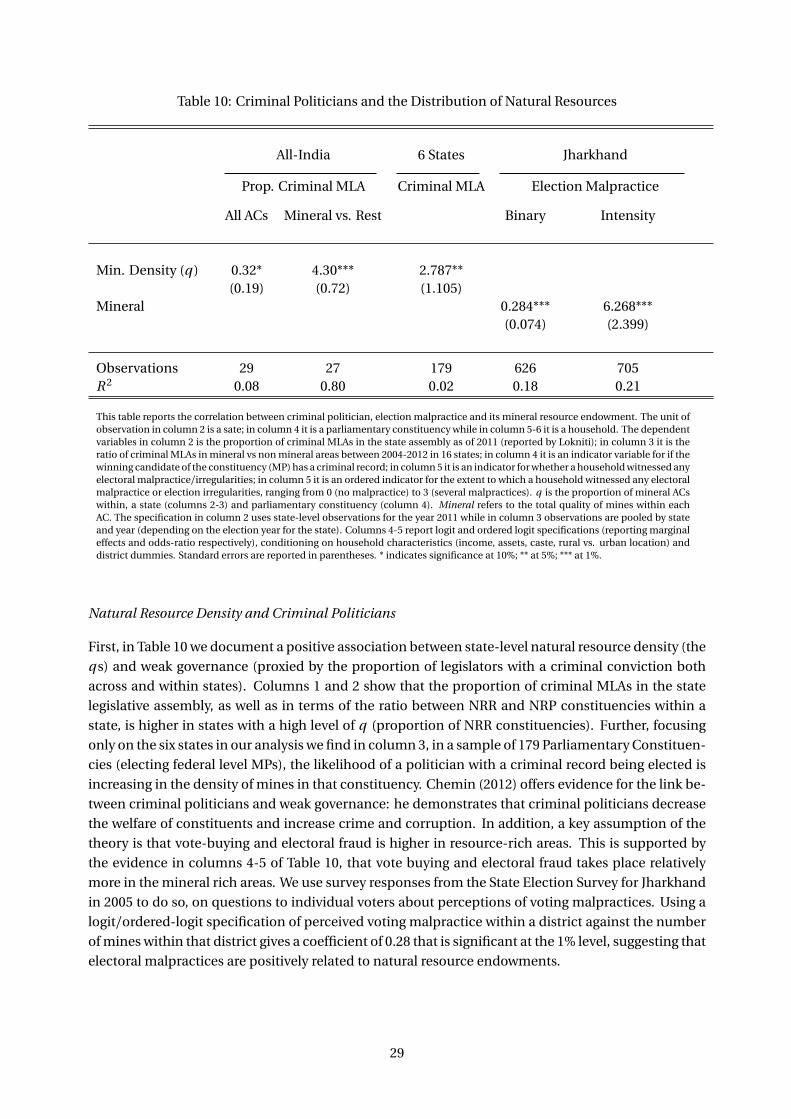
Table 10: Criminal Politicians and the Distribution of Natural Resources

All-India 6 States Jharkhand

Prop. Criminal MLA Criminal MLA Election Malpractice

All ACs Mineral vs. Rest Binary Intensity

Min. Density (q ) 0.32* 4.30*** 2.787**(0.19) (0.72) (1.105)

Mineral 0.284*** 6.268***(0.074) (2.399)

Observations 29 27 179 626 705R 2 0.08 0.80 0.02 0.18 0.21

This table reports the correlation between criminal politician, election malpractice and its mineral resource endowment. The unit ofobservation in column 2 is a sate; in column 4 it is a parliamentary constituency while in column 5-6 it is a household. The dependentvariables in column 2 is the proportion of criminal MLAs in the state assembly as of 2011 (reported by Lokniti); in column 3 it is theratio of criminal MLAs in mineral vs non mineral areas between 2004-2012 in 16 states; in column 4 it is an indicator variable for if thewinning candidate of the constituency (MP) has a criminal record; in column 5 it is an indicator for whether a household witnessed anyelectoral malpractice/irregularities; in column 5 it is an ordered indicator for the extent to which a household witnessed any electoralmalpractice or election irregularities, ranging from 0 (no malpractice) to 3 (several malpractices). q is the proportion of mineral ACswithin, a state (columns 2-3) and parliamentary constituency (column 4). Mineral refers to the total quality of mines within eachAC. The specification in column 2 uses state-level observations for the year 2011 while in column 3 observations are pooled by stateand year (depending on the election year for the state). Columns 4-5 report logit and ordered logit specifications (reporting marginaleffects and odds-ratio respectively), conditioning on household characteristics (income, assets, caste, rural vs. urban location) anddistrict dummies. Standard errors are reported in parentheses. * indicates significance at 10%; ** at 5%; *** at 1%.

Natural Resource Density and Criminal Politicians

First, in Table 10 we document a positive association between state-level natural resource density (the

q s) and weak governance (proxied by the proportion of legislators with a criminal conviction both

across and within states). Columns 1 and 2 show that the proportion of criminal MLAs in the state

legislative assembly, as well as in terms of the ratio between NRR and NRP constituencies within a

state, is higher in states with a high level of q (proportion of NRR constituencies). Further, focusing

only on the six states in our analysis we find in column 3, in a sample of 179 Parliamentary Constituen-

cies (electing federal level MPs), the likelihood of a politician with a criminal record being elected is

increasing in the density of mines in that constituency. Chemin (2012) offers evidence for the link be-

tween criminal politicians and weak governance: he demonstrates that criminal politicians decrease

the welfare of constituents and increase crime and corruption. In addition, a key assumption of the

theory is that vote-buying and electoral fraud is higher in resource-rich areas. This is supported by

the evidence in columns 4-5 of Table 10, that vote buying and electoral fraud takes place relatively

more in the mineral rich areas. We use survey responses from the State Election Survey for Jharkhand

in 2005 to do so, on questions to individual voters about perceptions of voting malpractices. Using a

logit/ordered-logit specification of perceived voting malpractice within a district against the number

of mines within that district gives a coefficient of 0.28 that is significant at the 1% level, suggesting that

electoral malpractices are positively related to natural resource endowments.

29

Natural Resource Density, Elections and Mining Intensity

Another perspective on the political channel is how the relative difference in outcomes for NRR ACs vs

NRP is affected by electoral competition. If a political channel is at work, this gap would vary over the

electoral cycle; and, if secession changes the political weight of NRR ACs as our theory says, we would

expect secession to change the way the gap is affected by the election cycle. The first two columns of

Table 11 show that this is the case: the coefficient we reported refers to the triple interaction of seces-

sion, mineral resource abundance at the AC level and election year (a triple difference-in-difference

effect). For Jharkand, we find a large and significant effect, which again points to the effects of seces-

sion operating through a political channel that flows through NRR ACs.

The third column of Table 11 focuses on how secession affects the gap between NRR ACs that are

swing ACs, in the sense that the fraction of voters who firmly support either party (partisan voters) is

small, and those where voters firmly support one party. Although our stylised theoretical discussion

has made no distinction between ACs along these lines, we might expect votes to be comparatively

more valuable in swing ACs, and so a higher “price” (x ) to be paid for votes in those ACs.42 The negative

and significant triple-interaction coefficient we see indicates that the negative effects of breakup in

NRR ACs for states which experience an increase in q post breakup are exacerbated when these ACs are

swing ACs. The fourth column of the table focuses instead on “politically aligned” NRR ACs where the

locally elected political belongs to the incumbent party at state level. We might expect that, when the

local politician is aligned with the ruling party, a vote-for-favours transaction might be easier, which

should exacerbate the adverse effects of secession in NRR ACs. The results of this triple interaction are

in line with this.

The theory also implies that mining-related activity should increase sharply in the new states that

see a large share of NRR areas post secession, because of more mining licenses being granted or be-

cause of increased opportunities for rent-seeking. Using data from the census of all firm establish-

ments in India between 1998 and 2005, we construct a measure of employment density in the mining

sector by taking the ratio of employment in the mining sector to the total employment of all sectors in

a particular district. Consistently with the prediction of an effect of secession on the relative intensity

of mining and non-mining activities, we find that the proportion of individuals employed in mining

increases by 0.14% post-secession in the NRR constituencies of the new states (Table 12).

Ruling Out Alternative Explanations

Our stylised model gives a precise characterisation of the effects of natural resource density that are

mediated by political competition; but the model’s predictions can be taken as being about the eco-

nomic effects of governance as broadly defined. In practice the way in which the quality of governance

is affected by a change in natural resource density in a particular case may materialise in ways other

than explicit granting of favours – e.g., what we might observe in a particular case, as a systematic re-

sponse to a higher density of NRR ACs, is a Chief Minister devoting insufficient attention to the man-

agement of natural resources. What we emphasise in our theory is the primacy of a political channel

42To see this, consider an asymmetric variation of our symmetric setup, in which there are two NRR constituencies, 1 and2, both having the same fraction, v , of votes for sale, but featuring electorates with different median ideologies. If 100% ofthe voters in AC 1 always support the incumbent irrespectively of whether or not votes are bought, then the votes that arefor sale in AC 1 have no value (or equivalently, they can be had for free), and therefore, an asymmetric equilibrium withconstituency-specific “prices” x1 and x2 will always feature x1 = 0. On the other hand, if 100% of the voters in AC 1 alwayssupport the challenger, then it may be prohibitively costly for the local seller to procure votes (i.e. there would be no votes forsale in that AC), and so again we would have x1 = 0. Thus, if resource rich ACs are aligned or swing ACs we expect outcomesto be worse post breakup, relative to non-aligned or non-swing ACs.

30

Table 11: Interactions with Political Indicators

Dependent variable: log light intensity

Electoral Cycle Election Factors

Bihar-Jharkhand

MadhyaPradesh-Chhattisgarh

Swing AC Political Alignment

Post ×New State ×Mineral × Election Year 35.301∗∗∗ −0.066(7.320) (0.980)

Post ×New State ×Mineral × Swing −4.278**(2.033)

Post ×New State ×Mineral × Alignment −1.973*(1.183)

Observations 5,688 3,096 11,034 9,195R 2 0.259 0.308 0.183 0.136

The table reports results for the effect of breakup on the log of light intensity within each AC, for a distance bandwidth of 250-200 km. The specification includes AC fixed effects, year fixed effects, border segment interacted with the Post indicator andcontrols for distance to the border by treatment status. All specifications also control for all possible interaction combinations,not reported, but which are mostly insignificant. Post refers to the years after breakup i.e., year 2001 onwards: New State is anindicator for the newly created state; Mineral refers to the total quality of mines within each AC; Elec Year refers to an indicator fortime t and t +1 where t is the identified election year; Swing refers to whether the margin of victory in the pre-breakup electionyear for less than 2%; Alignment is a (time-varying) binary indicator for whether the constituency’s winning candidate belongsto the (leading) ruling party of the state. The specification in Column 5, uses only observations prior to delimitation in 2008.Standard errors clustered at the AC level are reported in parentheses. * indicates significance at 10%; ** at 5%; *** at 1%.

31

Table 12: Mining Employment

% Mining Workers

Post ×New State 0.803(0.689)

Post −0.367(0.599)

Post ×Mineral −0.097∗

(0.051)

Post ×New State ×Mineral 0.135∗∗

(0.060)

Observations 74R 2 0.128

The table reports results for the effect of breakup on mining employment density in each district. % Min-ing Workers is the proportion of workers employed in the mining sector relative to the total employmentin a district. The specification includes, AC fixed effects, year fixed effects, border segment interacted withthe Post indicator and controls for distance to the border by treatment status. Post refers to the years afterbreakup i.e., year 2001 onwards: New State is an indicator for the newly created state; Mineral refers to thetotal quality of mines within each AC. Standard errors, clustered at the AC level, are reported in parentheses.* indicates significance at 10%; ** at 5%; *** at 1%.

mediating some of the effects of natural resource density that we observe.43

There are two main types of potentially competing explanations, not involving a link between pol-

itics and natural resources, that we must consider for the effects we see. First, a large literature has

looked at terms-of-trade effects associated with natural resource abundance (the “Dutch Disease”);

as the outcomes we consider are for regions that are part of a single economy where factors of pro-

duction can move freely across state borders, this type of explanation does not seem relevant for the

context we are studying.44 Second, it is possible that secession could bring about institutional or po-

litical changes that have nothing to do with natural resources; but, as Rodrik et al. (2004) argue, in-

stitutions are deep-seated, and so we could not expect them to have changed due to secession and

in such a short period. Changes in political outcomes coming from a change in the composition of

the electorate in the new states may well explain different outcomes overall, but cannot explain the

differential effect for NRR and NRP areas and how it relates to natural resource density.

Still, the effects that we observe to be associated with a large increase in natural resource density

could be due to state-level idiosyncratic factors that have nothing to do with the political channel we

describe; e.g. a Chief Minister may be a poor manager of natural resources independently of the mech-

43The literature has offered alternative characterisations of a politically-mediated natural resource curse, principalamongst them is one that focuses on windfall revenues leading to lower accountability and consequently higher moral haz-ard, worse selection and a higher likelihood of corrupt incumbents staying in power (Brollo et al. 2013). In our setting, thereare no windfall revenues to states – the windfall gain is just the higher share of mineral rich areas. Also, this explanation doesnot account for the differences between natural resource rich and poor areas at the local level.

44A related explanation is crowding out of other sectors by natural resources (e.g. Perroni and Proto 2010, plus others),but there is no reason to expect that this crowding out would be affected by secession – unless the effect operates through achange in the governance of natural resources.

32

Table 13: Ruling Out Other Determinants Correlated with Secession

Lights

BW 150 BW 150 BW 150

Post ×New State 0.381∗∗ -0.123 −0.095(0.168) (0.123) (0.160)

Post 2.037∗∗∗ −0.594∗∗∗ −0.620∗∗∗

(0.194) (0.085) (0.084)

Post ×Mineral 1.626∗∗ 1.014∗ 1.166∗∗

(0.773) (0.543) (0.565)

Post ×New State ×Mineral −2.758∗∗∗ −1.071∗ −1.232∗

(0.951) (0.647) (0.681)

Additional FEs – State×Year State×Election Year

Observations 9,720 9,720 9,720R 2 0.187 0.015 0.015

The table reports results for the effect of breakup on the log of total luminosity in each AC (columns 2-4)in each district (column 5). The specification includes, AC fixed effects, year fixed effects, border segmentinteracted with the Post indicator and controls for distance to the border by treatment status. BW refers tothe area bandwidth, used for selecting ACs on either side of the border for the analysis. Post refers to theyears after breakup i.e., year 2001 onwards: New State is an indicator for the newly created state; Mineralrefers to the total quality of mines within each AC. Standard errors, clustered at the AC level, are reportedin parentheses. Standard errors in columns 3-4 are additionally adjusted for auto-correlation. * indicatessignificance at 10%; ** at 5%; *** at 1%.

anism we describe. Although we cannot conclusively exclude that other factors may play a role, we

can amend our empirical specification to at least exclude those idiosyncratic state-level shocks that

are correlated with secession. Table 13 shows results for a specification that additionally conditions

on state-by-year effects (and state-by-election year); these controls accommodate any idiosyncratic

state-level shocks (such as a poor head of state or bad luck) that may be correlated with secession,

leaving only the secession-related structural break as the source of variation used to identify the ef-

fects. The inclusion of state-year effects reduces the effect of being in mineral-rich ACs in a new state,

but this effect remains statistically significant and negative.

Finally, a potential issue in the interpretation of the empirical results is the role of transfers from

the centre to the states upon breakup, which might have affected the evolution of outcomes over time.

However, as Figure 5 indicates, the pattern of transfers favours the old rump states, particularly Uttar

Pradesh.45 Although this picture cannot explain the relative success of Uttarakhand, it might explain

the relatively poor performance of the other two new states. But, as shown in Table 13, controlling for

state-specific time trends does not change the heterogeneity patterns we see, which emanates at the

more local level of the assembly constituencies.

45Note that the transfers measured here include all taxes, grants and loans to the state from the Centre.

33

Figure 5: Trends in Devolution and Transfer of Resources to New and Old States

The figure shows the amount (in INR crores) of money transfered from the center tothe new and old states between 1980-2010. Source: OpenBudgetIndia

7 CONCLUDING REMARKS

In this paper we exploit the breakup of three of the largest states in India, comprising areas with some

of the largest concentration of mineral resources in the country, to examine how changes in the po-

litical balance between natural resource related interests and other interests affects outcomes at the

local level. Our theoretical framework suggests that within a region where political opponents com-

pete with each other for votes, outcomes vary with the level of natural resource endowments: very

high endowments are likely to lead to perverse outcomes. The secession episode that occurred within

India allows us to examine this question using longitudinal evidence and in the context of a single

larger economy.

While the peculiarities of the Indian institutional context and the small number of secession cases

that we can compare across, as well as our regression discontinuity design, limit to some extent the

generalisability of our empirical results, the main predictions of the theory are consonant with the

patterns we find in the data. In particular, when new states inherit a large share of natural resources,

we see NRR areas in such states doing worse relative to comparable NRR areas in rump states and, in

comparative terms, doing worse than NRP areas of the same state. According to the theory presented

in Section 3, this is a symptom of a natural-resource curse that is mediated through a political channel.

While we cannot decisively rule out alternative explanations, a political channel seems the simplest

and most intuitive way to understand the evidence.

The question of how to design institutions that can harness the positive effects of natural resources

is an important one for economic development, as poorer countries rely comparatively more on nat-

ural capital (van der Ploeg 2011). Our results suggest that the adverse effects of patronage politics

could be mitigated by redrawing constituency borders so as to reduce the weight of NRR areas within

individual ACs and so make it more difficult to buy a large fraction of the total votes – although it has

been shown that vote trading is itself a function of the level of development (Aidt and Jensen 2017).

34

Second, our analysis suggests that outcomes might improve if the response to demands for secession

were met by higher fiscal redistribution towards the areas that threaten to secede, rather than by creat-

ing new political entities (although, of course, this may create a moral hazard problem). Indeed, Aidt

and Dutta (2016) shows the importance of the design of fiscal federalism institutions in the face of

different types of externalities between local regions. Finally, changing the current allocation of deci-

sion powers with respect to mineral concessions and royalty rates, as well as the way public revenues

from natural resources are allocated across state and local communities, may be an effective way of

mitigating the curse.46

References

Aidt, T., M. A. Golden, and D. Tiwari (2011). Incumbents and criminals in the Indian national legislature.Cambridge Working Papers in Economics 1157, University of Cambridge.

Aidt, T. S. and J. Dutta (2016). Fiscal federalism and electoral accountability. Journal of Public Economic The-ory 19(1), 38–58.

Aidt, T. S. and P. S. Jensen (2017). From open to secret ballot: Vote buying and modernization. ComparativePolitical Studies 50(5), 555–593.

Alesina, A., A. Devleeschauwer, W. Easterly, S. Kurlat, and R. Wacziarg (2003). Fractionalization. Journal ofEconomic Growth 8(2), 155–194.

Alesina, A., S. Michalopoulos, and E. Papaioannou (2016). Ethnic inequality. Journal of Political Econ-omy 124(2), 428–488.

Arjjumend, H. (2004). Tribal (land) rights and industry accountability: A case of mining in Jharkhand. Inno-vations in Civil Society (Participatory Research in Asia) 4(1).

Asher, S. and P. Novosad (2016). Dirty politics: Mining booms and political behaviour in India. mimeo.

Baland, J.-M. and P. Francois (2000). Rent-seeking and resource booms. Journal of Development Eco-nomics 61(2), 527–542.

Baskaran, T., B. Min, and Y. Uppal (2015). Election cycles and electricity provision: Evidence from a quasi-experiment with indian special elections. Journal of Public Economics 126, 64–73.

Bhandari, L. and K. Roychowdhury (2011). Night lights and economic activity in India: A study using DMSP-OLS night time images. Proceedings of the Asia-Pacific Advanced Network 32, 218–236.

Black, S. (1999). Do better schools matter? Parental valuation of elementary education. Quarterly Journal ofEconomics 114(2), 577–599.

Boffa, F., A. Piolatto, and G. Ponzetto (2016). Political centralization and government accountability. QuarterlyJournal of Economics 131(1), 381–422.

Brollo, F., T. Nannicini, R. Perotti, and G. Tabellini (2013). The political resource curse. American EconomicReview 103(5), 1759–1796.

Caselli, F. and G. Michaels (2013). Do oil windfalls improve living standards? Evidence from Brazil. AmericanEconomic Journal: Applied Economics 5(1), 208–38.

Chakraborty, L. S. and S. Garg (2015). The political economy of mining regulations 2015: Spatial inequalityand resource curse in two new states, India. Technical report.

Chakravorty, U., M. Pelli, and B. U. Marchand (2014). Does the quality of electricity matter? Evidence fromrural India. Journal of Economic Behavior & Organization 107(A), 228–247.

46The federal government that was instated in 2014 has proposed an amendment to the original Bill of 1957 that wouldaddress some of the problems we have mentioned – principal amongst them the excessive separation between the powersto set royalty rates and the powers to grant concessions – establishing District Mineral Foundations (DMFs) in areas affectedby mining related operations (Narain 2015). These new institutional arrangements might well hold the key to improved per-formance for areas with concentrated resources that might succumb to a local natural resource curse otherwise. However,the incentives for local capture of the DMFs cannot be readily discounted.

35

Chaturvedi, M., T. Ghosh, and L. Bhandari (2011). Assessing income distribution at the district level for Indiausing nighttime satellite imagery. Proceedings of the Asia-Pacific Advanced Network 32, 192–217.

Chauhan, S. S. (2010). Mining, development and environment: A case study of Bijolia mining area in Ra-jasthan, India. Journal of Human Ecology 31(1), 65–72.

Chen, X. and W. D. Nordhaus (2011). Using luminosity data as a proxy for economic statistics. Proceedings ofthe National Academy of Sciences 108(21), 8589–8594.

Collier, P. and A. Hoeffler (2006). The political economy of secession. In E. F. Babitt (Ed.), Negotiating selfdetermination, pp. 37–59. Lanham MD: Lexington Books.

Conley, T. G. (1999). GMM estimation with cross sectional dependence. Journal of Econometrics 92(1), 1–45.

Cust, J. and S. Poelhekke (2015). The local economic impacts of natural resource extraction. Annual Reviewof Resource Economics 7(1), 251–268.

de Melo, J., A. Panagariya, and D. Rodrik (1993). The new regionalism : a country perspective. In J. de Meloand A. Panagariya (Eds.), New Dimensions in Regional Integration. Cambridge University Press.

Dell, M. (2010). The persistent effects of Peru’s mining Mita. Econometrica 78(6), 1863–1903.

Desai, S., A. Dubey, B. Joshi, M. Sen, A. Shariff, R. Vanneman, and H. Codebook (2007). India human devel-opment survey (ihds). Computer file, icpsr22626-v2, University of Maryland, National Council of AppliedEconomic Research, New Delhi and Inter-University Consortium for Political and Social Research, Ann Ar-bor.

Fisman, R., F. Schulz, and V. Vig (2014). The private returns to public office. Journal of Political Econ-omy 122(4), 806–862.

Gomes, J. F. (2015). The political economy of the maoist conflict in India: An empirical analysis. World Devel-opment 68, 96–123.

Hahn, J., P. Todd, and W. Van der Klaauw (2001). Identification and estimation of treatment effects with aregression-discontinuity design. Econometrica 69(1), 201–209.

Henderson, J. V., A. Storeygard, and D. N. Weil (2011). A bright idea for measuring economic growth. AmericanEconomic Review 101(3), 194–199.

Imbens, G. and K. Kalyanaraman (2011). Optimal bandwidth choice for the regression discontinuity estima-tor. Review of Economic Studies 79(3), 933–959.

Imbens, G. W. and T. Lemieux (2008). Regression discontinuity designs: A guide to practice. Journal of Econo-metrics 142(2), 615–635.

Kulkarni, R., K. E. Haynes, R. R. Stough, and J. D. Riggle (2011). Revisiting night lights as proxy for economicgrowth: A multi-year light based growth indicator (LBGI) for China, India and the US. GMU School ofPublic Policy Research Paper (2011-12).

Kumar, A. (2010). Exploring the demand for new states. Economic and Political Weekly 45(33), 15–18.

Lokniti (2004). National election study 2004: An introduction. Economic and Political Weekly, 5373–5382.

Lowes, S., N. Nunn, J. A. Robinson, and J. L. Weigel (2017). The evolution of culture and institutions: Evidencefrom the Kuba kingdom. Econometrica 85(4), 1065–1091.

Mawdsley, E. (2002). Redrawing the body politic: Federalism, regionalism and the creation of new states inIndia. Commonwealth and Comparative Politics 40(3), 34–54.

McCrary, J. (2008). Manipulation of the running variable in the regression discontinuity design: A densitytest. Journal of Econometrics 142(2), 698–714.

Mehlum, H., K. Moene, and R. Torvik (2006). Institutions and the resource curse. Economic Journal 116(508),1–20.

Mitra, A., S. Mitra, and A. Mukherji (2017). Cash for votes: Evidence from India. University of Kent School ofEconomics Discussion Papers 1711, University of Kent.

Narain, S. (2015). The making of mining policy. The Business Standard.

Perroni, C. and E. Proto (2010). Entrepreneurial drain under moral hazard: A high-yield sector curse? Journalof Development Economics 93, 63–70.

Prakash, N., M. Rockmore, and Y. Uppal (2019). Do criminally accused politicians affect economic outcomes?evidence from india. Journal of Development Economics 141, 102370.

Rao, V. (1983). Crime in our society: A political perspective. Vikas.

36

Rodríguez-Pose, A. and M. Stermšek (2015). The economics of secession: Analysing the economic impact ofthe collapse of the former Yugoslavia. Territory, Politics, Governance 3(1), 73–96.

Rodrik, D., A. Subramanian, and F. Trebbi (2004). Institutions rule: The primacy of institutions over geographyand integration in economic development. Journal of Economic Growth 9(2), 131–165.

Rose, A. K. (2006). Size really doesn’t matter: In search of a national scale effect. Journal of the Japanese andInternational Economies 20(4), 482–507.

Rubinstein, A. (1982). Perfect equilibrium in a bargaining model. Econometrica 50(1), 97–109.

Sablik, T. (2015). The secession question: What are the economic costs and benefits of nations breaking apart?Econ Focus First Quarter, 12–16.

Sharma, K. (1976). Jharkhand movement in Bihar. Economic and Political Weekly, 37–43.

Singh, N. and B. Harriss-White (2019). The criminal economics and politics of black coal in Jharkhand, 2014.In B. Harriss-White and L. Michelutti (Eds.), The Wild East: Criminal Political Economies in South Asia.UCL Press.

Tillin, L. (2013). Remapping India: New states and their political origins. Hurst Publishers.

Vaishnav, M. (2017). When crime pays: Money and muscle in Indian politics. Yale University Press.

van der Ploeg, F. (2011). Natural resources: Curse or blessing? Journal of Economic Literature 49(2), 366–420.

Vanden Eynde, O. (2015). Mining royalties and incentives for security operations: Evidence from India’s RedCorridor. Technical report.

A DATA SOURCES

In this section we describe in detail the additional data used for the analysis.

National and State Election Study 2004: The survey is conducted by the CSDS. The survey interviews respon-dents immediately after polling and enumerates information on the political behaviour, opinion and attitudesof voters alongside their demographics. The survey uses a dummy ballot box for capturing the respondent’s vot-ing choice wherein respondents were asked to mark their voting preference on a dummy ballot paper and dropit in a dummy ballot box. Sampling for the survey is carried out using a multi-stage stratified random samplingdesign. The first stage involves stratified sampling of Assembly Constituencies by state proportional to theirsize. In the second stage, polling stations are sampled from each of these ACs, again proportional to electoratesize. In the final stage respondents are selected from the Electoral Rolls provided by the Election Commission.Respondents are sampled by the Systematic Random Sampling (SRS) method, which is based on a fixed inter-val ratio between two respondents in the polling booth. More information on the sampling and questionnairemodules of the 2004 NES can be found in Lokniti (2004).

AC and PC Maps: The Assembly Constituency (AC) and the Parliamentary Constituency (PC) map, shape fileswere obtained from the Election Commission of India website (http://eci.gov.in/). This data was cleaned andgeo-referenced using projections provided by Sandip Sukhtankar47 and INRM Consultants, New Delhi. Notethat the AC maps for Uttarakhand are only available post delimitation. However, only a small fraction of con-stituencies are affected by the delimitation procedure in Uttarakhand and are results are robust to droppingthese constituencies. Distances to the border for each AC was calculated by taking the centroid of each AC poly-gon and measuring its Euclidean distance to the state border line. Finally, we also divide the entire border lineinto segments which we include as fixed effects in our specifications.

Data on Conflict: The data on the conflict as measured by Maoist incidents is compiled by Gomes (2015)48 andcomes from four different sources: Global Terrorism Database (GTD) I: 1970-1997 & II: 1998-2007; Rand-MIPTTerrorism Incident database (1998-present); Worldwide Incidents tracking system (WITS); National CounterTerrorism Centre (2004-2007); South Asia Terrorism Portal (SATP).

47Retrieved from http://www.dartmouth.edu/~sandip/data.html.

48We are very grateful to Joseph Flavian Gomes for sharing his data on district level conflict in India.

37

Data on Criminal Politicians: Data on criminal politicians in India for the six states in our analysis is takenfrom Fisman et al. (2014), who compile this information from candidate affidavits. These are held on the theGENESYS Archives of the Election Commission of India (ECI) and the various websites of the the Chief ElectoralOfficer in each state. The archives provide scanned candidate affidavits (in the form of pictures or PDFs) for allcandidates. The all India data on criminal MLAs is taken from Prakash et al. (2019) (Table 10, Column 2) andLokniti (Table 10, Column 1).

Household Panel Data, IHDS: We use data from two waves (1992 and 2004) of the India Human DevelopmentSurvey (IHDS). This is a nationally representative survey of 41,554 households in 1,503 villages and 971 urbanneighbourhoods across India. Data are publicly available through ICPSR. For details on the survey see Desaiet al. (2007).

State Election Results: We use the results of all state elections held in the six states analysed, between the yearsof 1992 and 2009. This data is obtained from the Election Commission of India.

Human Demographics: We use data on district-level migration and literacy from the two census waves con-ducted in 1991 and 2001. This data is available on the census of India website.

Electricity Prices: Data on electricity tariff is compiled at an annual level for each state by India Stat.This data issourced from the annual reports on the working of state electricity boards and electricity departments as wellas the Planning Commission reports.

Firm Data: The census data on all firm establishments and employments activity in the mining sectors is ob-tained from the fourth (year 1998) and fifth (year 2005) round of the Economic Census. We supplement dataon firm level outcomes with information on wages and salaries and electricity consumption from the AnnualSurvey of Industries conducted in 2001.

B PROOFS

PROOF OF PROPOSITION 1

As only one buyer (the incumbent party, L) can buy votes, the votes for sale have no alternative use, and so ifthe buyer has all the bargaining power and can make a take-it-or-leave-it offer to the vote sellers, it will be ableto buy the votes at a price x = 0. On the other hand, if only the incumbent party, L , can buy votes, but the sellershave all the bargaining power and operate as a single seller (i.e. they collude), then the take-it-or-leave-it offerprice can be derived as follows.

The overall effect for a NRR constituency from x > 0 is given by (λ+ρq ) x , whereas the effect for a NRPconstituency is given by ρq x . The utility of voters in a NRR constituency from the L party being elected undershock s is now given byU L

i =−(−1/2−i+s )2−(λ+ρq ) x ,49 and a voter i is therefore indifferent between the L andR parties (i.e. U L

i =U Li ) iff−(−1/2−i+s )2−(λ+ρq )x =−(1/2−i+s )2. This gives the cutoff ideology conditional

on shock s as i N R R = −(λ+ρq )x/2− s , and in an NRP constituency the cutoff ideology is i N R P = −ρq x/2− s .The vote share of the L party among the 1 − v voters in q NRR constituencies who do not sell their votes isthen given by i N R R + 1/2 = 1/2− (1/2)(λ+ρq )x/2− s . The loss of votes due to x > 0 in an NRR constituencyis LR = (λ+ρq )x/2. The vote share of the L party among the voters in each of the 1− q NRP constituencies isgiven by i P +1/2, and the loss of votes in an NRP constituency due to x > 0 is LP =ρq x/2.

Suppose that party L buys the q v votes at price x in a state. The total vote share conditional on shocks is given by VL B = q v + q (1 − v ) (1/2− s − LR ) + (1 − q ) (1/2− s − LP ). The L party wins if VL B ≥ 1/2, i.e. iffq v + (1/2− s ) (1−q v ) +q (1− v ) (−LR )+ (1−q ) (−LP )≥ 1/2, or

q v

2−

q (1− v )λx

2− (1−q v )

ρq x

2≥ s (1−q v ). (7)

Using the fact that s is uniformly distributed on [−1/2, 1/2], the probability of winning is

P WL =

1

2+

1

2(1−q v )

�

q v −q (1− v )λx −ρq x (1−q v )�

≡Φ(x ). (8)

49Note that we ignore spillovers from other constituencies that are not in the state, as voters do not include those in thecalculation since they cannot affect those spillovers.

38

Then, the maximum price the buyer is willing to pay is that for which Φ(x ) = 1/2, which gives x = v /�

λ (1− v )+ρ (1− q v )

�

≡ x . The seller’s payoff, P WL x = Φ(x ) x , reaches a maximum at x = 2 x/(3 q v ), which, for v ≤ 1/2,

is always greater than x . Thus, x is the value of x that maximises the seller’s payoff subject to the constraintP W

L ≥ 1/2.

TWO BUYERS OR MULTIPLE SELLERS

If both the L and the R parties can buy votes from a single seller where the seller makes a simultaneous take itor leave it offer to the buyers, x remains unchanged. The sequence of actions is as follows. The seller posts aprice. Each buyer can accept or reject the price. If both buyers accept the offer, the votes are sold, at the postedprice, to one of the buyers selected at random. If one buyer accepts while the other buyer rejects, the acceptingbuyer gets the votes. If both buyers reject the offer, another offer can subsequently be made according to thesame protocol. We focus on subgame perfect equilibria of this game.

Allowing for multiple sellers also does not change conclusions, as the following discussion demonstrates.Suppose that there is a mass, q , of N NRR equal-sized constituencies, each of them having mass q/N ; andsuppose that sellers simultaneously post prices x1, x2, ...xN , and make a take it or leave it offer to the buyer. Eachseller chooses its price given the conjectured prices of the other sellers. If the seller of a single NRR constituency,j , sells v votes for a price x j , while all other sellers in NRR constituencies post a price x0 (assuming symmetry),the loss of votes (among the 1− v voters in the NRR districts) to the incumbent in constituency j is (1/2)

�

λx j +ρ�

x j +(N −1)x0

�

q/N�

. In the Natural Resource Poor (NRP) constituencies, the loss of votes is (1/2)ρ(x j +(N −1)x0)q/N . Hence the probability of winning is

P WL j =

1

2+

1

2(1−q v )

�

q v −q (1− v )�

λx j +ρ(x j + (N −1)x0

�

q/N − (1−q )�

ρ(x j + (N −1)x0

�

q/N�

. (9)

The best offer from the perspective of seller j is then that which makes the above expression equal to 1/2 (thebuyer’s reservation value), given the other sellers’ choice, x0. Solving for this optimal x j , as a function of x0,and then focusing on a symmetric solution with x j = x0, we obtain a value x that is the same as that with fullcollusion. The intuition for this result is that each seller, no matter how small, acts as a monopolist for its votesagainst the given buyer’s total reservation payoff of 1/2.

SEQUENTIAL BARGAINING

It can be shown that, under sequential bargaining, the equilibrium level of x is decreasing in ρ and increasingin q . The corresponding equilibrium values of P W

L are also decreasing in ρ and increasing in q .

Let U S (x ) =Φ(x ) x and U B (x ) =Φ(x )−1/2, and let�

U S (xS ),U B (xS )�

denote the offer made by the seller, and�

U S (xB ),U B (xB )�

the offer made by the buyer. If the seller is the first mover, an equilibrium corresponds to thesolution of the two equations: U B (xS ) =δU B (xB ) and U S (xB ) =δU S (xS ). This gives

xS = x1+δ

�

1+δ−p

1+δ(2+δ−4 q v (1−q v ))�

/(2v q )

1+δ+δ2. (10)

This is increasing in q. Thus, when some of the surplus accrues to the buyer (the incumbent party, L), an increasein the density of natural resources (a higher q ) can make the incumbent’s position more secure (it raises P W

L ).

Qualitatively analogous results obtain under Nash bargaining.

ENDOGENOUS q

Suppose than in any AC, j , there is a cost c for delivering v votes to the buyer. ACs are indexed so that theprivate net unit value, z ( j ), of the concessions made by the state in relation to natural resources (net of taxesand any other private costs incurred by the beneficiaries) is increasing in j , with j ∈ [0, 1]. Then the vote sellerwill deliver votes from a given AC, j , iff z ( j ) x > c , and will not deliver any votes from that AC otherwise. Sincez ′( j ) > 0, if z (0) x < c and z (1) x > c , there will be a cutoff point j (x ) such that there will be votes for sale onlyin ACs j > j , and so q = 1− j (x ). The seller’s take-it-or-leave it offer, x , together with the proportion, q , of ACs

39

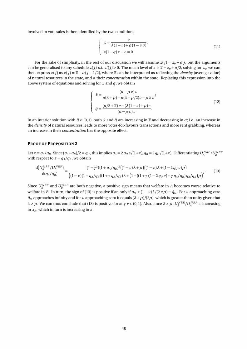
involved in vote sales is then identified by the two conditions

x =v

λ (1− v ) +ρ (1− v q );

z (1−q ) x − c = 0.(11)

For the sake of simplicity, in the rest of our discussion we will assume z ( j ) = z0 +α j , but the argumentscan be generalised to any schedule z ( j ) s.t. z ′( j )> 0. The mean level of z is z = z0+α/2; solving for z0, we canthen express z ( j ) as z ( j ) = z +α ( j − 1/2), where z can be interpreted as reflecting the density (average value)of natural resources in the state, and α their concentration within the state. Replacing this expression into theabove system of equations and solving for x and q , we obtain

x =(α−ρ c )v

α(λ+ρ)−α(λ+ρ/2)v −ρ z v;

q =(α/2+ z )v − (λ (1− v ) +ρ) c

(α−ρ c )v.

(12)

In an interior solution with q ∈ (0, 1), both x and q are increasing in z and decreasing in α; i.e. an increase inthe density of natural resources leads to more votes-for-favours transactions and more rent grabbing, whereasan increase in their concentration has the opposite effect.

PROOF OF PROPOSITION 2

Let z ≡ qA/qB . Since (qA+qB )/2= qU , this implies qA = 2 qU z/(1+z ), qB = 2 qU /(1+z ). DifferentiatingU N R PA /U N R P

Bwith respect to z = qA/qB , we obtain

d�

U N R PA /U N R P

B

�

d(qA/qB )=

(1−γ2) (1+qA/qB )2�

(1− v )λ+ρ� �

(1− v )λ+ (1−2 qU v )ρ�

�

(1− v ) (1+qA/qB ) (1+γqA/qB )λ+�

1+ ((1+γ)(1−2 qU v ) +γqA/qB )qA/qB

�

ρ�2 . (13)

Since U N R PA and U N R P

B are both negative, a positive sign means that welfare in A becomes worse relative to

welfare in B . In turn, the sign of (13) is positive if an only if qU < (1− v )λ/(2 v ρ) ≡ qU . For v approaching zero

qU approaches infinity and for v approaching zero it equals (λ+ρ)/(2ρ), which is greater than unity given that

λ >ρ. We can thus conclude that (13) is positive for any v ∈ (0, 1). Also, since λ >ρ, U N R RA /U N R P

A is increasing

in xA , which in turn is increasing in z .

40

C ADDITIONAL TABLES AND FIGURES

Table C1: RDD Estimates of Log Light Intensity, with Spatially Adjusted Errors

BW 150 BW 150 BW 150

Post ×New State 0.348*** 0.381***(0.103) (0.104)

Post × Jharkhand (new state) −0.855***(0.155)

Post × Chhattisgarh (new state) −0.324**(0.149)

Post ×Uttarakhand (new state) 1.444***(0.109)

Post

Post ×Mineral 1.626***(0.530)

Post ×New State ×Mineral −2.758***(0.635)

Observations 9,720 9,720 9,720R 2 0.042 0.070 0.043

The table reports results for the effect of breakup on the log of total luminosity in each AC. All specifica-tions include AC fixed effects, year fixed effects, border segment interacted with the Post indicator andcontrols for distance to the border by treatment status. BW refers to the area bandwidth, used for select-ing ACs on either side of the border for the analysis. Post refers to the years after breakup i.e., year 2001onwards: New State is an indicator for the newly created state; Mineral refers to the total quality of mineswithin each AC. Spatially adjusted standard errors are reported in parentheses. * indicates significanceat 10%; ** at 5%; *** at 1%.

41

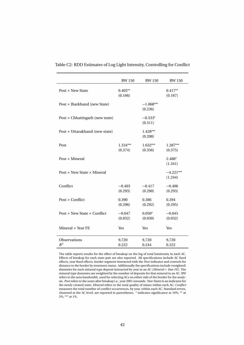
Table C2: RDD Estimates of Log Light Intensity, Controlling for Conflict

BW 150 BW 150 BW 150

Post ×New State 0.405∗∗ 0.417∗∗

(0.166) (0.167)

Post × Jharkhand (new State) −1.068∗∗∗

(0.236)

Post × Chhattisgarh (new state) −0.533∗

(0.311)

Post ×Uttarakhand (new state) 1.428∗∗∗

(0.208)

Post 1.334∗∗∗ 1.632∗∗∗ 1.287∗∗∗

(0.374) (0.356) (0.375)

Post ×Mineral 2.488∗

(1.341)

Post ×New State ×Mineral −4.221∗∗∗

(1.244)

Conflict −0.403 −0.417 −0.406(0.293) (0.290) (0.293)

Post × Conflict 0.390 0.386 0.394(0.296) (0.292) (0.295)

Post ×New State × Conflict −0.047 0.050∗ −0.045(0.032) (0.030) (0.032)

Mineral × Year FE Yes Yes Yes

Observations 9,720 9,720 9,720R 2 0.222 0.244 0.222

The table reports results for the effect of breakup on the log of total luminosity in each AC.Effects of breakup for each state-pair are also reported. All specifications include AC fixedeffects, year fixed effects, border segment interacted with the Post indicator and controls fordistance to the border by treatment status. Additionally the specifications include (weighted)dummies for each mineral type deposit interacted by year in an AC (Mineral × Year FE). Themineral type dummies are weighted by the number of deposits for that mineral in an AC. BWrefers to the area bandwidth, used for selecting ACs on either side of the border for the analy-sis. Post refers to the years after breakup i.e., year 2001 onwards: New States is an indicator forthe newly created state; Mineral refers to the total quality of mines within each AC; Conflictmeasures the total number of conflict occurrences, by year, within each AC. Standard errors,clustered at the AC level, are reported in parentheses. * indicates significance at 10%; ** at5%; *** at 1%.

42