second year syllabi i - semester ii - semesterece.anits.edu.in/second-year-syllabus.pdf ·...

SECOND YEAR SYLLABI

I - Semester

&

II - Semester

Second Year I –Semester

Code Subject name

Category Instruction periods per week Max marks

Credits Lecture Tutorial

Practi

cal Total

Sessional

marks

Semester

end marks

ECE 211 Engineering

Mathematics-III

BS 3 1 - 4 40 60 3

ECE 212 Electrical

Machines

ES 3 1 - 4 40 60 3

ECE 213 Data structures ES 3 1 - 4 40 60 3

ECE 214 Signals and

Systems

PC 3 1 - 4 40 60 3

ECE 215 Network analysis

and synthesis

ES 3 1 - 4 40 60 3

ECE 216 Electronic Circuits

and Analysis-I

PC 4 1 - 5 40 60 4

ECE 217

Electronic Circuits

and Analysis-I

Laboratory

PC

- - 3 3 50 50 2

ECE 218 Network & EM

Laboratory

ES - - 3 3 50 50 2

Total 19 6 6 31 340 460 23

Second Year II –Semester

*MOOCs: Course any time during 2-2 to 4-2. But its grade will be accorded with the 4-2 courses of the

program.

Code Subject name

Category

Instruction periods per week Max marks

Credits Lecture Tutorial

Practi

cal Total

Sessional

marks

Semester

end marks

ECE 221 Engineering

Mathematics –IV

BS 3 1 - 4 40 60 3

ECE 222 Electronic Circuits

and Analysis-II

PC 3 1 - 4 40 60 3

ECE 223 Digital Electronics PC 3 1 - 4 40 60 3

ECE 224

Probability Theory

and Random

Processes

PC

3 1 - 4 40 60 3

ECE 225

Electromagnetic

Field Theory &

Transmission Lines

PC

3 1 - 4 40 60 3

ECE 226 Control Systems ES 3 1 - 4 40 60 3

ECE 227

Electronic Circuits

and Analysis-II

Laboratory

PC

- - 3 3 50 50 2

ECE 228 Simulation

Laboratory

PC - - 3 3 50 50 2

Massive Open

Online Course

(MOOC)*

AC

- - - - - - -

Total 18 6 6 30 340 460 22

ENGINEERING MATHEMATICS –III ECE 211 Credits:3

Instruction: 3 Periods & 1 Tut/Week Sessional Marks:40

End Exam: 3 Hours End Exam Marks:60

Course Outcomes:

By the end of the course student should be able to:

1. Understanding the concepts of Gradient, Divergence and Curl and finding scalar potential

function of irrrotational vector fields.

2. Understanding the concepts of Green’s Theorem, Stokes’ Theorem and the Divergence

Theorem and to evaluate line integrals, surface, integrals and flux integrals.

3. Understand some basic techniques for solving linear partial differential equations and how to

identify a partial differential equation in order to determine which technique(s) can best be

applied to solve it.

4. Understand the methods to solve the Laplace, heat, and wave equations.

5. Gain good knowledge in the application of Fourier Transforms.

Mapping of Course Outcomes with Program Outcomes & Program Specific Outcomes:

SYLLABUS

UNIT-I VECTOR DIFFERENTIATION 12 Periods

Differentiation of Vectors – Scalar and Vector point function – Del applied to Scalar point functions

- Gradient geometrical interpretations – Directional Derivative - Del applied to vector point function

– divergence - Curl – Physical interpretation of Divergence and Curl - Del applied twice to point

functions- Del applied to product of point functions.

UNIT-II VECTOR INTEGRATION 12 Periods

Integration of vectors – Line integral – Surface – Green’s theorem in the plane – Stokes theorem –

Volume integral – Gauss Divergence theorems (all theorems without proofs) – Irrotational fields .

PO PSO

1 2 3 4 5 6 7 8 9 10 11 12 1 2 3

CO

1 3 2 - - - - - - - - - 2 2 - 3

2 3 1 - - - - - - - - - 2 2 - 3

3 3 1 - - - - - - - - - 2 2 - 3

4 3 2 - - - - - - - - - 2 2 - 3

5 3 2 - - - - - - - - - 2 2 - 3

UNIT-III PARTIAL DIFFERENTIAL EQUATIONS 12 Periods

Introduction – Formation of Partial Differential Equations – Solution of Partial Differential

Equations by Direct Integration – Linear Equations of the First order – Higher order Linear

Equations with Constant Co-efficients – Rules for finding the complementary function - Rules for

finding the Particular integral – Non- Homogeneous linear equations with constant coefficients.

UNIT –IV APPLICATIONS OF PARTIAL DIFFERENTIAL EQUATIONS 12 Periods

Introduction – Method of separation of variables – Vibrations of a stretched string- Wave equation –

One dimensional Heat flow - Two dimensional Heat flow – Solution of Laplace’s equation.-

Laplace’s equation in Polar Co-ordinates.

UNIT-V FOURIER TRANSFORMS 12 Periods

Introduction – definition – Fourier integral theorem - Fourier sine and cosine integrals – Complex

form of Fourier integrals – Fourier integral representation of a function – Fourier Transforms –

Properties of Fourier Transforms – Convolution Theorem – Parseval’s identity for Fourier

transforms – Fourier Transforms of the Derivatives of functions – Application of Transforms to

Boundary value problems – Heat conduction – Vibrations of a string.

Text Books:

1. Dr. B.S. Grewal, Higher Engineering Mathematics, 43rd

Edition, Khanna Publishers,

New Dehli, 2014.

Reference books:

1. A Text book on Engineering Mathematics by N.P. Bali Etal, Laxmi pub.(p)Ltd , 2001.

2. Advanced Engineering Mathematics by H.K.Dass , S.Chand Publications, 2007.

3. Advanced Engineering Mathematics by Erwin kreyszig, John Wiley Publications, 1999.

ELECTRICAL MACHINES ECE 212 Credits:3



Course Outcomes:


1. Find efficiency of DC Machine

2. Find Regulation and Efficiency of Single phase Transformer

3. Analyze the performance of Induction Motors

4. Understand working of synchronous machine

5. Understand basic concepts of Electric Power System


SYLLABUS

UNIT-I

DC Machines 18 Periods

Constructional Features, Function of Commutator, Induced EMF and Torque Expressions,

Relationship Between Terminal Voltage and Induced EMF for Generator and Motoring Action,

Different Types of Excitation and Performance Characteristics of Different Types of DC

Machines, Starting and Speed Control of DC Motors, Losses and Efficiency, Efficiency by

Direct Loading, Swinburne’s Test, and Applications of DC Machines.

UNIT -II 12 Periods

Transformers

Constructional Details, EMF Equation, Equivalent Circuit, Voltage Regulation, Losses and

Efficiency, Auto – Transformers, Open/Short – Circuit Tests and Determination of Efficiency

and Regulation.

UNIT-III 16 Periods

Induction Motors

Three-phase Induction Motors Rotating Magnetic Field, Construction of 3-ph Induction

Motor, Power Flow Diagram, Torque and Torque-slip Characteristics, Condition for Max.

PO PSO

1 2 3 4 5 6 7 8 9 10 11 12 1 2 3

CO

1 2 - - - - - - - - - - - 2

2 2 - - - - - - - - - - - 2

3 2 2 - - - - - - - - - - - 2

4 1 - - - - - - - - - - - 2

5 1 - - - - - - - - - - - 2

Torque and its Value, Starting methods of 3-phase Induction Motor, Losses and Efficiency,

Efficiency and Torque – Speed Characteristics.

Single-phase Induction Motors: Double Revolving Field Theory, Methods of Starting Single

Phase Induction Motors, Stepper Motor.

UNIT-IV 10 Periods

Three – Phase Synchronous Machines Generation of EMF, Constructional Details, Induced EMF, Synchronous Generator on No –

Load and Load, Synchronous Impedance and Voltage Regulation, Starting of Synchronous

Motors, Applications of Synchronous Machines.

UNIT-V 8 Periods

Electric Energy System (Elementary treatment only)

Single Line Diagram of AC Power supply systems, Types of Power Generation

sources(Conventional and Non – Conventional),Power Distribution Systems(Radial and Ring

Main Systems).

Text books:

1. J.B. Gupta, “Theory and Performance of Electrical Machines” , S. K. Kataria& Sons,

2009

2. P.S Bimbra, “Electrical Machinery”, Khanna Publications, 7th

Edition, 2009

3. V.K.Mehta, Rohit Mehta, “Principles of Power System”, S. Chand Publications,

4th

Edition, 2008

References:

1. Electrical Machines, S. K. Bhattacharya, TMH Publications N. Delhi.

DATA STRUCTURES ECE 213 Credits:3



Course Outcomes:


1 Demonstrate the knowledge in problem solving techniques.

2 Write programs for different data structures

3 Implement different applications using tree structures.

4 Implement various sorting techniques

5 Apply and implement learned algorithm design techniques and data structures to solve

problems using Graphs.


SYLLABUS

UNIT I

ARRAYS AND STACKS 12-Periods

Introduction: Basic Terminology, Elementary Data Organization, Data Structure operations,

Algorithm Complexity and Time-Space trade-off.

Arrays: Array Definition, Representation and Analysis, Single and Multidimensional Arrays,

address calculation, application of arrays, Character String in C, Character string operation,

Array as Parameters, Sparse Matrices.

Stacks: Array Representation and Implementation of stack, Operations on Stacks: Push & Pop,

Application of stack: Conversion of Infix to Prefix and Postfix Expressions, Evaluation of

Postfix & Prefix expressions using stack, Recursion, Towers Of Hanoi Problem.

UNIT II

QUEUES AND LINKED LIST 12 –Periods

Queues: Array representation and implementation of queues, Operations on Queue: Insert,

Delete, Full and Empty. Circular queue, De-queue, and Priority Queue, Applications of Queues.

Linked list: Representation and Implementation of Singly Linked Lists, Traversing and

Searching of Linked List, Insertion and deletion to/from Linked Lists, Doubly linked list,

Circular Doubly linked list, Implementing priority queue using Linked List, Polynomial

Representation using Linked list & addition.

PO PSO

1 2 3 4 5 6 7 8 9 10 11 12 1 2 3

CO

1 2 2 1 2 - - 2

2 2 1 - 2 - - 2

3 1 - 1 2 - - 2

4 1 - 1 2 - - 2

5 2 2 1 2 - - 2

UNIT III

TREES AND SEARCHING 12-Periods

Trees: Basic terminology, Binary Trees, Binary tree representation, Almost Complete Binary

Tree, Complete Binary Tree, Array and Linked Representation of Binary trees, Traversing

Binary trees, Threaded Binary trees.

Searching: Sequential search, binary search, Interpolation Search, comparison and analysis,

Hash Table, Hash Functions.

UNIT IV

BINARY SEARCH TREES AND BASIC SORTING TECHNIQUES 12-Periods

Sorting: Insertion Sort, Bubble Sort, Selection sort, Merge Sort.

Binary Search Trees: Binary Search Tree (BST), Insertion and Deletion in BST, Complexity of

Search Algorithm, AVL Trees.

UNIT V

GRAPHS 10-Periods

Graphs: Terminology & Representations- Graphs, Directed Graphs, Adjacency Matrices, Path

OR Transitive Closure of a Graph, Warshall’s Algorithm, Shortest path Algorithm-Dijkstra’s

Algorithm, Connected Component and Spanning Trees, Minimum Cost Spanning Trees,Graph

Traversals.

Text Books 1. Y. Langsam, M. Augenstin and A. Tannenbaum, “Data Structures using C and C++”,

Pearson Education, 2nd Edition, 1995.

2. Mark Allen Weiss, "Data Structures and Algorithm Analysis in C", Second Edition,

Pearson Education.

References: 1. E.Horowitz and Sahani, "Fundamentals of Data Structures"

2. C Programming and Data structures, P. Padmanabham, 3rd Edition, BS publications..

3. S. Lipschutz, “Data Structures”, McGraw Hill, 1986.

4. Programming in C , P. Dey & M. Ghosh, Oxford Univ. Press.

5. ISRD Group, “Data Structures through C++”, McGraw Hill, 2011.

SIGNALS AND SYSTEMS ECE 214 Credits:3



Course Outcomes:


1 Apply transformations on the independent variable of the given CT and DT signals and

analyze the properties of CT and DT signals and systems.

2 Represent mathematically the CT and DT LTI systems and determine the response of an

LTI system for the given input signal using either convolution integral or convolution

sum.

3 Represent CT and DT signals and systems in the Frequency domain using Fourier

Analysis tools like CTFS, CTFT, DTFS and DTFT.

4 Represent the CT signals in terms of its samples and reconstruct using interpolation.

5 Represent DT signals in the Frequency domain and analyze DT systems using Z-

Transforms and analyze CT signal and systems using Laplace transforms


SYLLABUS

Unit- I Introduction to Signals and Systems 10 Periods

Continuous-Time ( CT) signals and Discrete-Time ( DT) signals and their representation,

commonly used CT and DT signals: impulse, step, pulse, ramp and exponentials, classification

of CT and DT signals: periodic and aperiodic, even and odd, energy signals and power signals,

operations on CT and DT signals- addition, subtraction, multiplication, differentiation and

integration of CT signals, convolution and correlation of two signals ( CT& DT), properties of

convolution operation. Time-shifting and time-scaling of CT and DT signals, classification of CT

and DT systems: static and dynamic, linear and non-linear,time- invariant and time-varying,

basic concepts like causality,stability and invertability of systems.

Unit-II Linear Time-Invariant Systems 10 Periods

CT and DT type of LTI systems, impulse response function and unit-sample response sequence,

Input-Output relation through convolution summation/ integral, characterization of CT and DT

types of LTI systems, impulse response function/ sequence and causalitity of LTI systems,

interconnectected LTI systems ( CT and DT), CT type of LTI systems described by Linear

PO PSO

1 2 3 4 5 6 7 8 9 10 11 12 1 2 3

CO

1 2 1 - - - - - - - - - - 2 2 -

2 2 2 - - - - - - - - - - 2 2 -

3 2 1 - - - - - - - - - - 3 2 -

4 2 2 - - - - - - - - - - 2 2 -

5 2 1 - - - - - - - - - - 2 2 -

constant coefficient differential equations, DT type LTI systems described by constant

coefficient linear difference equations, BIBO stability of LTI systems ( CT and DT types).

Unit III Analysis of CT Signals and Systems 12 Periods

Fourier series analysis of CT Signals, CT Fourier transform( FT) and its inverse; magnitude and

phase spectra, FT using impulses, FT as a particular case of Laplace Transform(LT), FT and LT

in CT system analysis, magnitude and phase responses of CT type LTI systems, block diagram

representation of Linear Differential Equations with constant coefficients, pole-zero locations,

causality (Paley- Wiener Criterion )and stability, distortionless transmission of signals through

CT type LTI systems.

Unit IV Analysis of DT Signals and Systems 15 periods

Discrete –time Fourier transform( DTFT) & inverse DTFT; convergence of DTFT and IDTFT;

DTFT properties and theorems, discrete Fourier transform (DFT)& inverse DFT; properties and

theorems, circular convolution, Z-Transform( ZT) & its properties & theorems, inverse ZT,

inversion methods power series, PFE and Residue methods, solution of difference equations

using ZT, distortionless transmition through DT type of LTI systems, ROCs of right-sided, left

sided and finite duration sequences, relationship between ZT, DTFT and DFT.

Application of ZT, DTFT and DFT in DT signal and system analysis, DT system function,

transfer function, poles and zeros, stability, block diagram representation of difference equations,

processing of CT signals using DFT.

Unit V Sampling of Lowpass and Bandpass Signals 10 periods

Lowpass sampling theorem and its proof, types of sampling: impulse sampling, natural sampling

and flat-top sampling, spectra of sampled vertions, aliasing, Nyquist rate, anti-aliasing filter,

reconstruction of band – limited lowpass signal from its samples, aperture effect due to flat- top

sampling, reconstruction filters and zero – order hold( ZOH), sampling of bandpass signals and

bandpass sampling theorem.

Text Books :

1. A.V. Oppenheim, AS Willsky and S.H. Nawab: Signals and Systems, Pearson.

2. S.Haykin and B.V Veen: Signals and Systems, John Wiley

References:

1. P. Ramakrishna Rao and Shankar Prakriya : Signals and Systems, second addition, McGraw

Hill ( India) pvt Ltd. 2013

2. Nagoor Kani: Signals and Systems, McGraw Hill

3. E.W Kamen and B.S.Heck: Fundamentals of Signals and Systems using the Web and Matlab,

Pearson.

4. P. Ramesh Babu and R. Anandanatarajan: Signals and Systems 4/e, Scitech.

5. K. Raja Rajeswari and B. Visveswara Rao: Signals and Systems , PHI.

NETWORK ANALYSIS AND SYNTHESIS ECE 215 Credits:3



Course Outcomes:


1 Apply basic network theorems and analyze both D.C and A.C. circuits.

2 Determine various parameters of two port networks.

3 Analyze circuits under resonant condition.

4 Calculate natural and forced response of RL, RC & RLC circuits

5 Measure real, reactive, apparent power in three phase circuits.


SYLLABUS

UNIT-I

ANALYSIS OF DC CIRCUITS 10 periods

Active Element, Passive Element, Reference Directions For Current and Voltage, Kirchoff’s

Laws, Voltage and Current Division, Nodal Analysis, Mesh Analysis, Linearity and

Superposition, Thevenin's and Norton’s Theorems, Source Transformation.

UNIT-II

DC TRANSIENTS 12 periods

Inductor, Capacitor, Source Free RL, RC & RLC Response, Evaluation of initial

Conditions, Application of Unit-Step Function to RL, RC & RLC Circuits, Concepts of

Natural, Forced and Complete Response.

UNIT-III

SINUSOIDAL STEADY-STATE ANALYSIS 14 periods The Sinusoidal Forcing Function, Phasor, Instantaneous and Average Power, Complex

Power, Steady State Analysis Using Mesh and Nodal Analysis, Application of Network

Theorems to A.C. Circuits.

PO PSO

1 2 3 4 5 6 7 8 9 10 11 12 1 2 3

CO

1 3 1 1 3 1 -

2 3 1 2 1 1 -

3 2 2 2 3 2 2

4 3 1 2 1 - 1

5 2 2 3 2 1 2

UNIT-IV

RESONANCE &COUPLEDCIRCUITS 12periods

Balanced Three Phase Circuits, Resonance, Concept of Duality. Coupled Circuits:

Magnetically Coupled Circuits, Dot Convention.

UNIT-V

NETWORK SYNTHESIS 10 periods

Elementary synthesis operation, LC network synthesis, Properties of RC network functions,

Foster and Cauer forms of RC and RL networks.

Text books:

1. W.H. HAYT Jr & J.E. KEMMERLY, "ENGINEERING CIRCUIT ANALYSIS, 5th

Edition, Mc. Graw Hill Pub.

2. M.E. VAN VALEKNBURG, "NETWORK ANALYSIS", 3rd Edition, PHI Learning.

Reference book:

1. Circuits and Networks by A. Sudhakar Shyammohan S Palli, 4th

Edition, TMH Publication.

ELECTRONIC CIRCUITS AND ANALYSIS-I ECE 216 Credits:4



Course Outcomes:


1 Determine the performance parameters like current gain, voltage gain, input impedance,

output impedance using the models such as h-parameter model, simplified CE h –

parameter model and π-model.

2 Analyze the frequency response characteristics of single stage and multistage amplifier

circuits (i.e. given a lower cut off, upper cut-off frequencies of an amplifier determining

the coupling and bypass capacitor values) and different circuit configurations for

improving the transistor amplifier characteristics such input impedance, voltage gain etc.

3 Analyze the response of linear wave shaping circuits such as high pass and low pass filter

circuits for different types of inputs such as step input, pulse input, square input ramp

input.

4 Analyze the response of Non-linear wave shaping circuits such as clipping and clamping

circuits when the sinusoidal input is applied and to design two level clipping circuits in

order to select the desired portion of the input signal.

5 Determine the stable state voltages and currents and design the various multivibrators to

meet the given specifications.


SYLLABUS

Unit-I

Transistor at low frequencies and high frequencies 12 periods

Graphical analysis of CE configuration, Two port devices and hybrid model, Transistor hybrid

model, h-parameters, conversion formulas of three transistor configurations, Analysis of

transistor amplifier circuit using h-parameters, the emitter follower, Millers theorem and its dual,

cascading transistor amplifiers, simplified CE hybrid model, high input resistance transistor

circuits, hybrid- π CE transistor model, hybrid- π conductance, hybrid- π capacitances, validity

and variation of hybrid- π parameters.

PO PSO

1 2 3 4 5 6 7 8 9 10 11 12 1 2 3

CO

1 3 2 - - - - - - - - - - - 2

2 3 2 2 - - - - - - - - - - 2

3 3 2 - - - - - - - - - - - -

4 3 2 - - - - - - - - - - - -

5 3 2 2 - - - - - - - - - - 2

Unit-II

Multistage Amplifiers 8 periods

Classification of amplifiers, Distortion in amplifiers, Frequency response of an amplifier, The

RC coupled amplifier-low frequency response, high frequency response of two cascaded CE

stages, Band- pass of cascaded stages, Cascode amplifiers, Multistage CE amplifier cascade at

High frequencies.

Unit-III

Linear wave shaping 12 periods

The high pass RC circuit, High pass RC circuit as a differentiator, Double differentiation, The

low pass RC circuit, Low pass RC circuit as an integrator, attenuators, RL and RLC circuits.

Unit-IV

Clipping and Clamping Circuits 12 periods Diode Clippers, The transistor clipper, Clipping at two independent levels, Cathode coupled and

emitter coupled clipper, Compensation for temperature changes, comparators, breakaway diode

and amplifier, diode differentiator comparator, accurate time delays, applications of voltage

comparator, The clamping operation, clamping circuit taking source and diode resistance into

account, Clamping circuit theorem, Practical clamping circuits, effect of diode characteristics on

clamping voltage, Synchronized clamping.

Unit-V

Multivibrators 12 periods

Stable stages of a binary, fixed bias transistor binary, self bias transistor binary, commutating

capacitors, methods of improving resolution, emitter coupled binary, Schmitt trigger circuit, the

monostable multivibrator, emitter coupled monostable multivibrator, astable emitter coupled

multivibrator.

Text Books:

1. Jacob Millman, Christos Halkias, Chetan Parikh, "Integrated Electronics", 2nd Edition,

McGraw Hill Publication, 2009.[unit1,unit2]

2. Jacob Millman & Herbert Taub, “Pulse Digital & Switching Waveforms” McGraw-Hill

Book Company Inc.[unit3,unit4,unit5]

References:

1. Donald A. Neamon, “Electronic Circuit Analysis and Design”, 2nd

Edition. TMH

publications.

ELECTRONIC CIRCUITS AND ANALYSIS-I LABORATORY

ECE 217 Credits:2

Instruction: 3 Practical’s / Week Sessional Marks:50


Course Outcomes:


1 Measure the important parameters of a PN diode and to implement for various

Applications.

2 Design and construct different rectifier and voltage regulation circuits used in regulated

Power supplies.

3 Design amplifier circuits for specific applications, based on their input and output

Characteristics of BJT and FET.

4 Design and verify the output of linear wave shaping circuits for different inputs.

5 Design and analyze different multivibrator circuits.


LIST OF EXPERIMENTS

Cycle-I Design and simulation using MultiSim software

1. Plot the V-I characteristics of a PN diode in forward and reverse bias and find the static,

dynamic resistances and the reverse saturation current.

2. Plot the V-I characteristics and regulation characteristics of a Zener diode in reverse bias.

3. Plot the output waveforms of a halfwave rectifier and find the ripple factor.

4. Plot the output waveforms of a fullwave rectifier using 2 diodes.

5. Plot the output waveforms of a Bridge rectifier and find the ripple factor.

6. Low pass and High pass circuits

7. Clippers and Clampers circuit

8. Plot the input and output characteristics of CE configured transistor and to find the h-

parameter values from the characteristics.

9. Plot the input and output characteristics of CB configured transistor and to find the h-


10. Plot the input and output characteristics of CC configured transistor and to find the h-


11. Plot the drain and transfer characteristics of a JFET.

12. Plot the frequency response of a single stage CE amplifier.

PO PSO

1 2 3 4 5 6 7 8 9 10 11 12 1 2 3

CO

1 1 - 1 3 2 - - - - - - - 2 2 1

2 2 - 2 3 2 - - - - - - - 2 2 1

3 2 - 2 3 2 - - - - - - - 2 2 1

4 2 - 2 3 2 - - - - - - - 2 2 1

5 2 - 2 3 2 - - - - - - - 2 2 1

13. Plot the frequency response of a single stage CC amplifier.

14. Verify the working of a BJT as a switch.

15. Frequency Response of a RC coupled multistage amplifier

16. Study the operation of a Bistable multivibrator and observe the switching action.

17. Astable Multivibrator

18. Monostable Multivibrator

19. Observe the hysteresis loop of a Schmitt trigger circuit

20. Design and implement a DC regulated power supply.

Cycle-II (Hardware experiments)

1. Plot the V-I characteristics of a PN diode in forward and reverse bias and find the static,

dynamic resistances and the reverse saturation current.

2. Plot the V-I characteristics and regulation characteristics of a Zener diode in reverse bias.

3. Plot the output waveforms of a halfwave rectifier and find the ripple factor.

4. Plot the output waveforms of a fullwave rectifier using 2 diodes.

5. Plot the output waveforms of a Bridge rectifier and find the ripple factor.

6. Plot the input and output characteristics of CE configured transistor and to find the h-


7. Plot the input and output characteristics of CB configured transistor and to find the h-


8. Plot the drain and transfer characteristics of a JFET.

9. Verify the working of a BJT as a switch.

10. Plot the frequency response of a single stage CE amplifier.

11. Plot the frequency response of a single stage CC amplifier.

12. Study the operation of a Bistable multivibrator and observe the switching action.

13. Observe the hysteresis loop of a Schmitt trigger circuit

Text Books:


McGraw Hill Publication, 2009.

2. Jacob Millman & Herbert Taub, “Pulse Digital & Switching Waveforms” McGraw-Hill

Book Company Inc.

References:


Edition. TMH

publications.

NETWORK & EM LABORATORY ECE 218 Credits:2

Instruction: 3 Practical’s / Week Sessional Marks:50


Course outcomes:


1 Conduct the experiments based on basic network theorems.

2 Predict the characteristics of D.C machines and single phase transformers

3 Predict the regulation of an alternator.


LIST OF EXPERIMENTS

CYCLE-I: Networks Lab

1. To obtain filament lamp characteristics.

2. Verification of KCL & KVL.

3. Verification of superposition theorem.

4. Verification of Thevenin’s and Norton’s theorem.

5. Determination of two port network parameters.

CYCLE-II: Electrical Machines Lab

1. O.C.C & Load characteristics of D.C shunt generator.

2. Swinburne’s test on D.C. shunt machine.

3. Brake test on D.C. shunt motor.

4. O.C. & S.C test on a single phase transformer.

5. Brake test on 3-phase induction motor.

6. Regulation of alternator by e.m.f. method.

Textbooks:

1. W.H.Haytjr & J.E.Kemmerly , “Engineering Circuit Analysis” , 5th Edition, Mc. Graw Hill

Pub.

2. J.B. Gupta, “Theory and Performance of Electrical Machines” ,S. K. Kataria& Sons, 2009

PO PSO

1 2 3 4 5 6 7 8 9 10 11 12 1 2 3

CO

1 3 1 1 3 - 1 - - - - - - 3 - 2

2 3 2 - 3 - 2 - - - - - - 2 1 1

3 2 1 1 3 - 1 - - - - - 2 1 1

ENGINEERING MATHEMATICS –IV ECE 221 Credits:3



Course Outcomes:


1

Understand, interpret and use the basic concepts: Analytic function, harmonic function,

Taylor and Laurent Series, Singularity, Residues and evaluation of improper integrals.

2 Familiarize the concepts of Finite Differences and Interpolation techniques.

3 Familiarize the concept of Differentiation and Integration by numerical methods.

4 Understand the characteristics and properties of Z-transforms and its applications.

5 Analyze the Statistical data by using statistical tests and to draw valid inferences about the

population parameters.


SYLLABUS

UNIT-I FUNCTIONS OF A COMPLEX VARIABLE 14 Periods

Introduction –Limit of a Complex function- Derivative of – Analytic functions-Harmonic

functions - Applications to Flow problems. Complex Integration- Cauchy’s Theorem- Cauchy’s

Integral Formula –Series of Complex terms ( Statements of Taylor’s and Laurent’s Series without

proof ) - Zeros of an Analytic function - Residues - Calculation of Residues - Evaluation of Real

Definite Integrals ( Integration around the unit circle, Integration around the small semi circle ,

Indenting the Contours having poles on the real axis).

Geometric representation of , Some standard transformation

(

) .

UNIT-II FINITE DIFFERENCES & INTERPOLATION 12 Periods

Finite Differences – Forward differences – Backward differences – Central differences –

Differences of a Polynomial – Factorial Notation – Other difference operators – To find one or

more missing terms – Newton’s Interpolation Formulae – Central Difference Interpolation

Formulae - Interpolation with Unequal Intervals – Lagrange’s interpolation formula – Inverse

Interpolation.

PO PSO

1 2 3 4 5 6 7 8 9 10 11 12 1 2 3

CO

1 2 1 - - - - - - - - - - 2 - 1

2 2 1 - - - - - - - - - - 2 - 1

3 2 1 - - - - - - - - - - 2 - 1

4 2 1 - - - - - - - - - - 2 - 1

5 2 1 - - - - - - - - - - 2 - 1

UNIT-III NUMERICAL DIFFERENTIATION AND INTEGRATION 10 Periods

Numerical Differentiation – Formulae for derivatives – Maxima and Minima of a Tabulated

Function – Numerical Integration – Newton-Cotes Quadrature Formula – Trapezoidal rule –

Simpson’s One-Third rule , Simpson’s Three-Eighth rule.

UNIT - IV Z – TRANSFORMS 12 Periods

Introduction – Definition - Some Standard Z-Transforms –Linearity Property –Damping Rule – Some

Standard Results - Shifting Un to the right , Shifting Un to the left – Two basic theorems ( Initial

Value Theorem and Final Value Theorem) – Convolution Theorem – Convergence of Z-transforms –

Two sided Z - transform of Un - Evaluation of inverse Z- transforms ( Power Series Method , Partial

Fraction Method , Inverse integral method ) - Applications to Difference equations.

UNIT-V SAMPLING THEORY 12 Periods

Introduction – Sampling Distribution – Testing a hypothesis – Level of Significance –

Confidence Limits – Test of Significance of Large samples (Test of significance of single mean,

difference of means) – Confidence limits for unknown – Small samples – Students t-distribution

– Significance test of a sample mean – Significance test of difference between sample means –

Chi-Square ( ) Test – Goodness of fit.

Text Books:

1. Dr. B.S. Grewal, Higher Engineering Mathematics, 43rd

Edition, Khanna Publishers,

New Dehli, 2014.

Reference books:

1. N.P. Bali Etal, “A Text book on Engineering Mathematics”, Laxmi pub.(p) Ltd , 2011.

2. H.K.Dass “Advanced Engineering Mathematics”, S.Chand Publications, 2007.

3. Erwin kreyszig, “Advanced Engineering Mathematics”, John Wiley Publications, 1999.

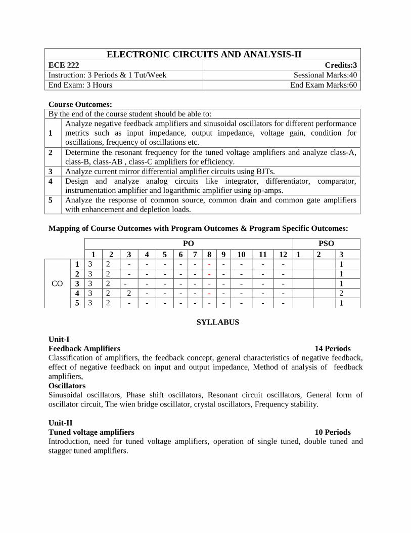
ELECTRONIC CIRCUITS AND ANALYSIS-II ECE 222 Credits:3



Course Outcomes:


1

Analyze negative feedback amplifiers and sinusoidal oscillators for different performance

metrics such as input impedance, output impedance, voltage gain, condition for

oscillations, frequency of oscillations etc.

2 Determine the resonant frequency for the tuned voltage amplifiers and analyze class-A,

class-B, class-AB , class-C amplifiers for efficiency.

3 Analyze current mirror differential amplifier circuits using BJTs.

4 Design and analyze analog circuits like integrator, differentiator, comparator,

instrumentation amplifier and logarithmic amplifier using op-amps.

5 Analyze the response of common source, common drain and common gate amplifiers

with enhancement and depletion loads.


SYLLABUS

Unit-I

Feedback Amplifiers 14 Periods

Classification of amplifiers, the feedback concept, general characteristics of negative feedback,

effect of negative feedback on input and output impedance, Method of analysis of feedback

amplifiers,

Oscillators

Sinusoidal oscillators, Phase shift oscillators, Resonant circuit oscillators, General form of

oscillator circuit, The wien bridge oscillator, crystal oscillators, Frequency stability.

Unit-II

Tuned voltage amplifiers 10 Periods

Introduction, need for tuned voltage amplifiers, operation of single tuned, double tuned and

stagger tuned amplifiers.

PO PSO

1 2 3 4 5 6 7 8 9 10 11 12 1 2 3

CO

1 3 2 - - - - - - - - - - 1

2 3 2 - - - - - - - - - - 1

3 3 2 - - - - - - - - - - 1

4 3 2 2 - - - - - - - - - 2

5 3 2 - - - - - - - - - - 1

Power Amplifiers Class A Large Signal amplifiers, Second Harmonic Distortion, Higher order Harmonic

Distortion, The Transformer coupled audio power amplifier, Efficiency, Push-Pull amplifiers,

Class B Amplifiers, Class AB operation, Class C amplifier.

Unit-III

Differential amplifiers 10 Periods

The Differential amplifier, Basic BJT differential pair, DC transfer characteristic, small signal

equivalent circuit analysis, differential and common mode gain, differential and common mode

impedances, Bipolar transistor current sources, two transistor current sources, improved current

source circuits, Widlar current source, multi transistor current mirrors.

Unit-IV

Applications of Operational Amplifiers: 10 Periods

Review of basics of Op-Amp, Basic op-amp applications, Differential DC amplifier, Stable AC

coupled amplifier, Analog Integration and differentiation, comparators, sample and hold circuits,

Precision AC/DC converters, Logarithmic amplifiers, waveform generators, regenerative

comparators, Instrumentation amplifier.

Unit-V

FET Amplifiers 12 Periods

MOSFET DC circuit analysis, The MOSFET amplifier - small signal equivalent circuit,

Common source amplifier, source follower amplifier, Common Gate amplifier. NMOS

amplifiers with enhancement load, depletion load and PMOS load, CMOS source follower and

common gate amplifiers.

Text Books:


McGraw Hill Publication, 2009.[unit-1,unit-2,unit-4]


Edition. TMG

publications. [unit-3,unit-5]

References:

1. Ramakanth A Gayakwad, “Op-Amps and Linear Integrated Circuits”- 4th Edition.

DIGITAL ELECTRONICS ECE 223 Credits:3



Course Outcomes:


1

Perform number conversions between different number systems and codes and apply

Boolean algebra to minimize logic expressions up to three variables.

2 Analyze the characteristics of logic families and compare their performance in terms of

performance metrics.

3 Apply tabulation method to minimize logic expressions up to Five variables and design a

combination logic circuit like decoders, encoders, multiplexers, and de-multiplexers etc.

for a given specification and verify the correctness of the design.

4 Analyze the operation of sequential circuits built with various flip-flops by finding the

Boolean function or truth table and design various sequential circuits like flip-flops,

registers, counters etc.

5 Design of sequential detector by constructing a state/output tables or diagrams from a word

description or flow chart specification of sequential behavior using either mealy and/or

Moore machines.„


SYLLABUS

UNIT-I 10 periods

NUMBER SYSTEMS: Number representation, Conversion of bases, Binary Arithmetic,

Representation of Negative numbers, Binary codes: weighted and non-weighted, Error detecting

and correcting codes -- Hamming codes.

BOOLEAN ALGEBRA: Basic definitions, Axiomatic Definitions, Theorems and properties,

Boolean Functions, Canonical and standard forms.

UNIT-II 10 periods

LOGIC FAMILIES

PO PSO

1 2 3 4 5 6 7 8 9 10 11 12 1 2 3

CO

1 1 1 1 - - - - - - - - - 3 - 2

2 1 2 2 - - - - - - - - - 3 - 2

3 1 2 2 - - - - - - - - - 3 - 2

4 1 2 2 - - - - - - - - - 3 - 2

5 1 2 2 - - - - - - - - - 3 - 2

Binary Logic, AND, OR, NOT, NAND, NOR, EX-OR and Equivalence gates. Introduction,

Specifications of digital circuits, RTL and DTL circuits, Transistor-Transistor Logic (TTL),

Emitter Coupled Logic (ECL), MOS, CMOS circuits, Performance comparison of logic families.

UNIT-III 14 periods

GATE-LEVEL MINIMIZATION

The Map Method: Two variable map, Three variable map, four variable map, Prime Implicants,

Don't care conditions, NAND and NOR implementation, Exclusive-OR Function, Parity

Generation and Checking, Variable Entered Mapping (VEM): Plotting Theory, Reading Theory,

Quine-Mccluskey (QM) Technique.

COMBINATIONAL LOGIC

Combinational circuits, Analysis Procedure, Design procedure, Binary Adder-Subtractor,

Decimal adder, carry look ahead adder, Binary Multiplier, Magnitude comparator, Decoders,

Encoders, Multiplexers, ROM, PLA, PAL.

UNIT-IV 14 periods

SYNCHRONOUS SEQUENTIAL LOGIC

Block diagram of sequential circuit, Latches, Flip-flops, Triggering of Flip-flops, Flip-flop

excitation tables, Analysis of clocked sequential circuits, State equations, state table, state

diagram, analysis with D, JK and T-Flip-flops, state machines, state reduction and assignment,

Design procedure.

REGISTERS AND COUNTERS

Registers, Shift registers, universal shift register Ripple counters, Synchronous counters, counter

with unused states, Ring counters, Johnson counter.

UNIT-V 12 periods

ASYNCHRONOUS SEQUENTIAL LOGIC

Analysis Procedure, Circuits with latches, Design procedure, Reduction of state and flow tables,

cycles, Race-Free state Assignment, Hazards, Design example.

Text Books:

1. M. Morris Mano, Digital Design, 3rd

Edition, Pearson Publishers, 2001.

2. Z Kohavi, Switching and Finite Automata Theory, 2nd edition, TMH, 1978

Reference Books:

1. William I. Fletcher, An Engineering Approach to Digital Design, PHI, 1980.

2. John F. Wakerly, Digital Design Principles and Practices, 3rd Edition, Prentice Hall, 1999.

3. Charles H Roth Jr and Larry L. Kinney, Fundamentals of Logic Design, Cengage learning,

7th Edition, 2013

4. R.P Jain, Modern Digital Electronics, 3rd Edition, TMH, 2003.

PROBABILITY THEORY AND RANDOM PROCESSES ECE 224 Credits:3



Course Outcomes:


1 Calculate probabilities and conditional probabilities of events defined on a sample space.

2 Compute statistical averages of one random variables using probability density and

distribution functions and also transform random variables from one density to another

3 Compute statistical averages of two or more random variables using probability density

and distribution functions and also perform multiple transformations of multiple random

variables.

4 Determine stationarity and ergodicity and compute correlation and covariance of a

random process.

5 Compute and sketch the power spectrum of the response of a linear time-invariant system

excited by a band pass/band-limited random process.


SYLLABUS

UNIT-I Probability and Random Variable 12Periods

Probability: Probability introduced through Sets and Relative Frequency, Experiments and

Sample Spaces, Discrete and Continuous Sample Spaces, Events, Probability Definitions and

Axioms, Mathematical Model of Experiments, Probability as a Relative Frequency, Joint

Probability, Conditional Probability, Total Probability, Bayes’ Theorem, Independent Events.

Random Variable: Definition of a Random Variable, Conditions for a Function to be a Random

Variable, Discrete, Continuous and Mixed Random Variables.

UNIT –II Distribution & Density Functions and Operation on One Random Variable

12 Periods

Distribution & Density Functions: Distribution and Density functions and their Properties -

Binomial, Poisson, Uniform, Gaussian, Exponential, Rayleigh and Conditional Distribution,

Methods of defining Conditional Event, Conditional Density, and Properties.

Operation on One Random Variable: Introduction, Expected Value of a Random Variable,

Function of a Random Variable, Moments about the Origin, Central Moments, Variance and

PO PSO

1 2 3 4 5 6 7 8 9 10 11 12 1 2 3

CO

1 3 3 3 2 2 2 1

2 3 3 3 2 2 2 1

3 3 3 2 2 2 1

4 3 3 2 2 2 1

5 3 3 1 2 2 1

Skew, Chebychev’s Inequality, Characteristic Function, Moment Generating Function,

Transformations of a Random Variable: Monotonic Transformations for a Continuous Random

Variable, Non-monotonic Transformations of Continuous Random Variable, Transformation of a

Discrete Random Variable.

UNIT-III Multiple Random Variables and Operations 12 Periods

Multiple Random Variables: Vector Random Variables, Joint Distribution Function, Properties

of Joint Distribution, Marginal Distribution Functions, Conditional Distribution and Density –

Point Conditioning, Conditional Distribution and Density – Interval conditioning, Statistical

Independence, Sum of Two Random Variables, Sum of Several Random Variables, Central

Limit Theorem (Proof not expected), Unequal Distribution, Equal Distributions.

Operations on Multiple Random Variables: Expected Value of a Function of Random

Variables: Joint Moments about the Origin, Joint Central Moments, Joint Characteristic

Functions, Jointly Gaussian Random Variables: Two Random Variables case, N Random

Variable case, Properties, Transformations of Multiple Random Variables, Linear

Transformations of Gaussian Random Variables.

UNIT-IV Random Process - Temporal Characteristics 12 periods

Introduction, The Random Process Concept: Classification of Process, Deterministic and

Nondeterministic Process. Stationary and Independence: Distributions and Density Functions,

Statistical Independence, First-order Stationary Process, Second-Order and Wide-sense

Stationary, N-Order and Strict-Sense Stationary, Time Averages and Ergodicity, Mean-Ergodic

Process, Correlation-Ergodic Process. Correlation Functions: Autocorrelation Functions and Its

Properties, Cross-correlation Functions and its properties, Covariance Functions, Discrete-Time

Process and Sequences. Measurement of Correlation Functions, Guassian Random Process,

Poisson Random Process, Complex Random Process.

UNIT-V Spectral Analysis 12 periods

The Power Spectrum, Linear System, Hilbert Transform, Discrete Time Process, Modulation:

Rice’s Representation, Band pass processes, Band limited Processes and Sampling Theory.

Text Book:

1. Probability, Random Variables & Random Signal Principles - Peyton Z. Peebles, 4Ed., 2001,

McGraw Hill.

2. Probability, Random Variables and Stochastic Processes – Athanasios Papoulis and S.

Unnikrishna Pillai, McGraw Hill, 4th Edition, 2002.

Reference Book:

1. Probability Theory and Random Processes, S. P. Eugene Xavier, S. Chand and Co. New

Delhi, 1998 (2nd Edition).

2. Probability, Statistics, and Random Processes for Engineers- Henry Stark & John W. Woods,

4Ed, 2012, Pearson

3. Introduction to Random Signals and Noise, Davenport W. B. Jrs. and W. I. Root, McGraw

Hill N.Y., 1954.

ELECTROMAGNETIC FIELD THEORY & TRANSMISSION LINES ECE 225 Credits:3



Course Outcomes:


1 Apply vector calculus to static electric fields in different engineering situations

2 Solve the problems related to magnetostatic fields by applying magnetostatic laws.

3 Analyze Maxwell’s equation in different forms (differential and integral) and apply them

to diverse engineering problems.

4 Analyze the phenomena of wave propagation in different media.

5 Apply the concepts of transmission line and use smith chart to find various parameters

useful to design a matching circuits at radio frequency


SYLLABUS

UNIT I Electrostatics 14 periods

Introduction to vector analysis, Fundamental of electrostatic fields, Different types of charge

distributions, Coulomb’s law and Electric field intensity, Potential function, Equi-potential

surface, Electric field due to dipole; Electric flux density, Gauss’s law and applications,

Poisson’s and Laplace’s equations and its applications; Uniqueness theorem; Boundary

conditions; Conductors & Dielectric materials in electric field; Current and current density,

Relaxation time, Relation between current density and volume charge density; Dipole moment,

Polarization, Capacitance, Energy density in an electric field.

UNIT II Steady Magnetic Fields 12 periods Introduction, Faradays law of induction, Magnetic flux density, Biot-Savart law, Ampere’s

circuit law, Magnetic Force, Magnetic Boundary conditions, Scalar and Vector magnetic

potentials, Magnetization & Permeability in materials, Inductance, Energy density, Energy stored

in inductor.

UNIT III Maxwell’s Equations 10 periods Introduction, Faradays law, displacement current, Equation of continuity for the varying fields,

inconsistency of Amperes circuit law, Maxwell’s equations in integral form, Maxwell’s

PO PSO

1 2 3 4 5 6 7 8 9 10 11 12 1 2 3

CO

1 3 2 1 2 2 2 1

2 3 2 1 2 2 2 1

3 3 2 1 3 2 2 2

4 3 2 1 2 2 2 2

5 3 2 3 3 2 2 3

equations in point form, retarded potentials Meaning of Maxwell’s equations, conditions at a

Boundary surfaces, Retarded potentials.

UNIT IV Electromagnetic Waves 10 periods Introduction, Applications of EM waves, solutions for free space condition ,; Uniform plane

wave propagations uniform plane waves, wave equations conducting medium, sinusoidal time

variations, conductors & dielectrics, Depth of penetration, Direct cosines, Polarization of a

wave, reflection by a perfect conductor – Normal incidence, Oblique incidence, reflection by a

perfect dielectric-Normal incidence, reflection by a perfect insulator – oblique, Surface

impedance, Poynting vector and flow of power, Complex poynting vector.

UNIT V Transmission Lines 10 periods

Types of transmission lines, Applications of transmission lines, Equivalent circuit of pair of

transmission lines, Primary constants, Transmission line equations, Secondary constants, lossless

transmission lines, Distortionless line, Phase and group velocities, Loading of lines, Input

impedance of transmission lines, RF lines, Relation between reflection coefficient, Load and

characteristic impedance, Relation between reflection coefficient and voltage standing wave ratio

(VSWR), Lines of different lengths - 2,4,8 lines, Losses in transmission lines, Smith chart

and applications, Stubs, Double stubs.

Text Books:

1. E.C. Jordan and K.G. Balmain, “Electromagnetic Waves and Radiating Systems”, PHI, 2nd

Ed., 2000.

2. William H. Hayt Jr. and John A. Buck, “Engineering Electromagnetics”, TMH, 7th Ed., 2006.

Reference Books:

1. G.S.N.Raju, Electromagnetic Field Theory And Transmission Lines, Pearson Education

(Singapore) Pvt., Ltd., New Delhi, 2005.

2. M.N.O. Sadiku, “ Principles of Electromagnetics”, Oxford International Student edn., 4th

edn., 2007.

3. G. Sasi Bhushana Rao, “Electromagnetic Field Theory andTransmission Lines”, Wiley, India

Pvt. Ltd, 2012.

4. Simon Ramo, et.al-, “Fields and waves in communication electronics”, Wiley India Edn.,

3rd

Edn., 1994

CONTROL SYSTEMS ECE 226 Credits:3



Course Outcomes:


1 Apply block reduction techniques and signal flow graphs

2 Apply mathematical modelling of mechanical and electrical systems

3 Analyze the given systems in time domain

4 Determine the relative and steady state stability of the systems

5 Analyze the systems in frequency domain


SYLLABUS

UNIT-I Introduction to Control Systems 12 Periods

Transfer Functions of Linear Systems - Impulse Response of Linear Systems-Block

Diagrams of Control Systems-Signal Flowgraphs (Simple Problems) - Reduction Techniques

for Complex Block Diagrams and Signal Flow Graphs (Simple Examples).

UNIT-II Modeling of Control Systems 10 periods

Introduction to Mathematical Modelling of Physical Systems - Equations of Electrical

Networks - Modelling of Mechanical Systems - Equations of Mechanical Systems.

UNIT-III Time domain analysis 16 periods

Time Domain Analysis of Control Systems - Time Response of First and Second Order

Systems with Standard Input Signals-Steady State Performance of Feedback Control

Systems-Steady State Error Constants-Effect of Derivative and Integral Control on Transient

and Steadystate Performance of Feedback Control Systems.

UNIT-IV Concept of stability in time domain 12 periods

Concept of Stability and Necessary Conditions for Stability - Routh - Hurwitz Criterion,

Relative Stability Analysis, The Concept and Construction of Root Loci, Analysis of Control

Systems With Root Locus (Simple Problems to Understand Theory)

PO PSO

1 2 3 4 5 6 7 8 9 10 11 12 1 2 3

CO

1 1 - - - - - - - - - - - - - 2

2 1 - - - - - - - - - - - - - 2

3 2 1 - - - - - - - - 1 - 1 - 2

4 2 1 - - - - - - - - 1 - 1 - 2

5 2 2 - - - - - - - - 1 - 1 - 2

UNIT-V Frequency domain analysis 14 periods Correlation Between Time and Frequency Responses - Polar Plots - Bode Plots - Log

Magnitude Versus Phase Plots-All Pass and Minimum Phase Systems-Nyquist Stability

Criterion-Assessment of Relative Stability-Constant M&N Circles.

Text books:

1. I.J. Nagrath & M.Gopal, “Control systems engineering”, wiley eastern limited.

2. Benjamin C. Kuo, “Automatic control systems”, prentice hall of India

References:

1. Ogata, “Modern control engineering”, prentice hall of India.

ELECTRONIC CIRCUITS AND ANALYSIS-II LABORATORY ECE 227 Credits:2

Instruction: 3 Practical’s /Week Sessional Marks:50


Course outcomes:


1 Design and identify the applications of feedback amplifiers and sinusoidal oscillators in

different electronic circuits.

2 Design and implement different power amplifiers and tuned voltage amplifiers.

3 Calculate the parameters of BJT differential amplifier.

4 Apply op-amps fundamentals in design and analysis of op-amps applications.

5 Apply the MOSFET inverter in different electronic circuits.


LIST OF EXPERIMENTS

1. Obtain the input and output impedance of a trans-conductance amplifier with and without

feedback.

2. Obtain the frequency response of a voltage shunt negative feedback amplifier with and

without feedback.

3. Generate a sinusoidal signal using Colpitts oscillator at a desired frequency.

4. Generate a sinusoidal signal using Wein bridge circuit.

5. Generate a sinusoidal signal using RC phase shift oscillator and observe the lissajous

patterns at different phase shifts.

6. Plot the frequency response of a tuned voltage amplifier and find the resonant frequency.

7. Obtain the output waveforms of a class-B pushpull power amplifier and calculate the

efficiency and distortion.

8. Obtain the output waveforms of a class-A transformer coupled power amplifier and calculate

the power conversion efficiency.

9. Determine the gain and CMRR for the BJT differential amplifier.

10. Obtain the signals at the output junctions of multistage BJT differential pair.

11. Verify different applications of an Operational amplifier.

12. Verify different parameters of an operational amplifier.

13. Observe the working of an operational amplifier in inverting, non inverting and differential

modes.

14. Plot the V-I characteristics of an n-channel enhancement MOSFET and verify its operation

as an inverter.

PO PSO

1 2 3 4 5 6 7 8 9 10 11 12 1 2 3

CO

1 2 2 2 2 - - - - - 2 - - 2 - 2

2 2 2 2 2 - - - - - 2 - - 2 - 2

3 1 2 2 1 - - - - - 2 - - 2 - 2

4 2 2 3 2 - - - - - 2 - - 2 - 2

5 2 1 2 2 - - - - - 2 - - 2 - 2

15. Verify the working of a CMOS source follower amplifier.

Text books:


McGraw Hill Publication, 2009.


Edition. TMG

publications.

References:

1. Ramakanth A Gayakwad, “Op-Amps and Linear Integrated Circuits”- 4th Edition.

SIMULATION LABORATORY ECE 228 Credits:2

Instruction: 3 Practical’s /Week Sessional Marks:50


Course outcomes:


1 Calculate the convolution and correlation between signals

2 Plot magnitude and phase spectrum of a given signal using various transformation tools.

3 Generate random sequences for a given distribution.

4 Understand the basics of VHDL and describe the logic circuit using different types of

models in the architecture of the body.

5 Design and simulate combinational and sequential circuits using VHDL


LIST OF EXPERIMENTS

Cycle-I (MATLAB)

1 Basic Operations on Matrices.

2 Write a program for Generation of Various Signals and Sequences (Periodic and

Aperiodic), such as Unit impulse, unit step, square, saw tooth, triangular, sinusoidal,

ramp, sinc.

3 Write a program to perform operations like addition, multiplication, scaling, shifting, and

folding on signals and sequences and computation of energy and average power.

4 Write a program for finding the even and odd parts of signal/ sequence and real and

imaginary parts of signal.

5 Write a program to perform convolution between signals and sequences.

6 Write a program to perform autocorrelation and cross correlation between signals and

sequences.

7 Write a program for verification of linearity and time invariance properties of a given

continuous/discrete system

8 Write a program for computation of unit samples, unit step and sinusoidal response of

the given LTI system and verifying its physical realiazability and stability properties.

9 Write a program to find the Fourier transform of a given signal and plotting its

magnitude and Phase spectrum.

10 Write a program for locating the zeros and poles and plotting the pole-zero maps in S

plane and Z-plane for the given transfer function.

11 Write a program for Sampling theorem verification.

PO PSO

1 2 3 4 5 6 7 8 9 10 11 12 1 2 3

CO

1 2 - - 1 3 - - - - 2 - - 2 2 1

2 2 - - 1 3 - - - - 2 - - 2 2 1

3 2 - - 1 3 - - - - 2 - - 2 2 1

4 2 - - 1 3 - - - - 2 - - 2 2 1

5 2 - 3 1 3 - - - - 2 - - 2 2 2

12 Write a program for Removal of noise by autocorrelation / cross correlation.

13 Generation of random sequence

14 Write a program to generate random sequence with Gaussian distribution and plot its pdf

and CDF .

15 Write a program for verification of winer- khinchine relations.

16 Let Z be the number of times a 6 appeared in five independent throws of a die. Write a

program to describe the probability distribution of Z by:

Plotting the probability density function

Plotting the cumulative distribution function

17 Plot the probability mass function and the cumulative distribution function of a

geometric distribution for a few different values of the parameter p. How does the shape

change as a function of p?

18 Write a program to generate 10,000 samples of an exponentially distributed random

variable using the simulation method. The exponential random variable is a standard one,

with mean 10. Plot also the distribution function of the exponentially distributed random

variable using its mathematical equation.

19 Write a program to determine the average value and variance of Y=exp(X), where X is a

uniform random variable defined in the range [0, 1]. Plot the PDF of Y

20 Consider the random process defined as X[n] = 2U [n] − 4U [n − 1], where U [n] is a

white noise with zero mean and variance σ2 = 1. Generate a realization of 1000 samples

of X[n] by using MATLAB. Based on this realization, estimate the power spectral

density and plot the estimate.

Cycle-II (VHDL modeling and simulation of the following experiments using ModelSim)

1. Realization of logic gates

2. Verifying the functionality of half adder and full adder using basic gates and universal

gates.

3. Verifying the functionality of half subtractor and full subtractor using basic gates and

universal gates.

4. Design of 4-bit magnitude comparator

5. Design of Multiplexers/De-multiplexers

6. Decoders , Encoders

7. Code converters

8. Verifying the functionality of JK,D and T- Flipflops

9. Design of synchronous counter using the given type of flip flop

10. Design of asynchronous counter using the given type of flip flop

Note: A minimum of any ten experiments have to be done from cycle-I and any six

experiments from cycle-II

Text Books:

1. Rudra Pratap, “Getting Started with MATLAB: A Quick Introduction for Scientists &

Engineers ” Oxford 2010.

2. J Bhaskar,”VHDL Primer” 3rd Edition ,Prentice Hall 1999

References:

1. J G Proakis, VK Ingle, "Digital signal processing using MATLAB", 3rd

Edition, Cengage

learning.

second year syllabi i - semester ii - semesterece.anits.edu.in/second-year-syllabus.pdf ·...

Documents