Section 1.4

Intersection of Straight Lines

Intersection Point of Two Lines

Given the two lines 1 1 1

2 2 2

:

:

L y m x b

L y m x b

m1 ,m2, b1, and b2 are constants

Find a point (x, y) that satisfies both equations.

Solve the system consisting of

L1

L2

1 1 2 2 and y m x b y m x b

Ex. Find the intersection point of the following pairs of lines:

4 7

2 17

y x

y x

Notice both are in Slope-Intercept Form

4 7 2 17x x Substitute in for y

6 24

4

x

x

Solve for x

Find y4 7

4(4) 7 9

y x

Intersection point: (4, 9)

Break-Even AnalysisThe break-even level of operation is the level of production that results in no profit and no loss.

Profit = Revenue – Cost = 0

Revenue = Cost

Dollars

Units

loss

Revenue

Cost

profit

break-even point

Cost: C(x) = 3x + 3600

Ex. A shirt producer has a fixed monthly cost of $3600. If each shirt has a cost of $3 and sells for $12 find the break-even point.

If x is the number of shirts produced and sold

Revenue: R(x) = 12x( ) ( )

12 3 3600

400

R x C x

x x

x

(400) 4800R

At 400 units the break-even revenue is $4800

Market Equilibrium

Market Equilibrium occurs when the quantity produced is equal to the quantity demanded.

price

x units

supply curve

demand curve

Equilibrium Point

Ex. The maker of a plastic container has determined that the demand for its product is 400 units if the unit price is $3 and 900 units if the unit price is $2.50. The manufacturer will not supply any containers for less than $1 but for each $0.30 increase in unit price above the $1, the manufacturer will market an additional 200 units. Both the supply and demand functions are linear. Let p be the price in dollars, x be in units of 100 and find:

a. The demand function

b. The supply function

c. The equilibrium price and quantity

a. The demand function

, : 4,3 and 9,2.5 ;x p3 2.5

0.14 9

m

3 0.1 4p x

0.1 3.4p x

b. The supply function

, : 0,1 and 2,1.3 ;x p 1 1.30.15

0 2m

0.15 1p x

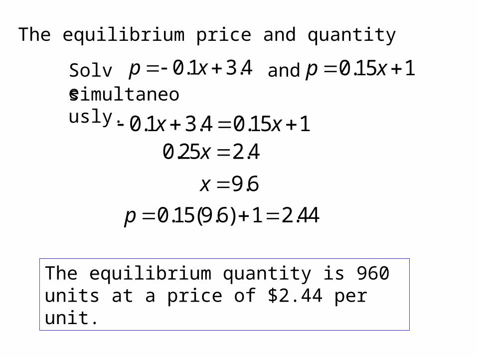
c. The equilibrium price and quantity

Solve 0.1 3.4p x 0.15 1p x and simultaneously.

0.1 3.4 0.15 1x x 0.25 2.4

9.6

x

x

The equilibrium quantity is 960 units at a price of $2.44 per unit.

0.15(9.6) 1 2.44p