Section 3.3

If the space of a random variable X consists of discrete points, then X is said to be a random variable of the discrete type. If the space of a random variable X is a set S consisting of an interval (possibly unbounded) of real numbers or a union of such intervals, then X is said to be a random variable of the continuous type. The probability density function (p.d.f.) of a continuous type random variable X is an integrable function f(x) satisfying the following conditions:

(1)

(2)

(3)

f(x) > 0 for x S (Note: for convenience, we may allow S to contain certain discrete points where f(x) = 0.)

f(x) dx = 1

S

P(A) = P(X A) = f(x) dx

A

i.e, P(a < X < b) = f(x) dx

a

b

Suppose X is a continuous-type random variable with outcome space S and p.d.f f(x).

The mean of X is

The variance of X is

The standard deviation of X is

x f(x) dx = E(X) = .

(x – )2f(x) dx = E[(X – )2] =

2 = Var(X) .

E[X2 – 2X + 2] = E(X2) – 2E(X) + E(2) =

E(X2) – 22 + 2 = E(X2) – 2 =

= Var(X) .

Recall that for any random variable X, the cumulative distribution function (c.d.f.) of X is defined to be F(x) = P(X x). If X is a continuous-type random variable, we may write F(x) =

S

S

–f(t) dt

x

The Fundamental Theorem of Calculus implies F /(x) = f(x).

For a continuous-type random variable X with outcome space S and p.d.f f(x), we can define the following:

The m.g.f. of X (if it exists) is

and (just as with discrete-type random variables)

The (100p)th percentile of the distribution of X, where 0 < p < 1,

is defined to be a number p such that

The median of the distribution of X is defined to be

The first, second, and third quartiles of the distribution of X are defined to be

M(t) = E(etX) = etx f(x) dx

S

M(n)(0) = E(Xn).

0.5 .

0.25 , 0.5 , and 0.75 respectively.

F(p) = p.

1.

(a)

(b)

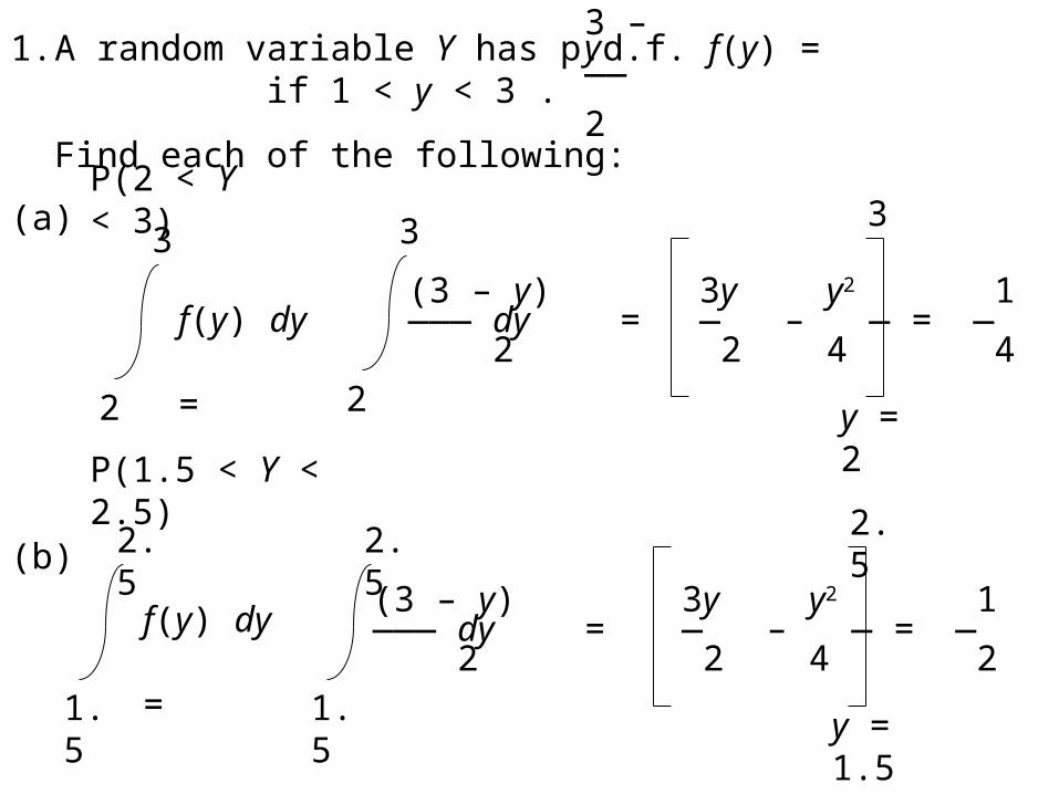
A random variable Y has p.d.f. f(y) = if 1 < y < 3 .

Find each of the following:

P(2 < Y < 3)

3 – y—— 2

2

3

f(y) dy =

2

3

(3 – y)——— dy = 2

3y y2

— – — = 2 4

y = 2

3

1— 4

P(1.5 < Y < 2.5)

1.5

2.5

f(y) dy =

1.5

2.5

(3 – y)——— dy = 2

3y y2

— – — = 2 4

y = 1.5

2.5

1— 2

(c)

(d)

P(Y < 2)

E(Y)

–

2

f(y) dy =

1

2

(3 – y)——— dy = 2

3y y2

— – — = 2 4

y = 1

2

3— 4

–

y f(y) dy =

1

3

(3 – y)y ——— dy = 2

1

3

(3y – y2)———— dy = 2

3y2 y3

— – — = 4 6

y = 1

3

5— 3

(e) Var(Y)

E(Y2) =

–

y2 f(y) dy =

1

3

(3 – y)y2 ——— dy = 2

1

3

(3y2 – y3)———— dy = 2

3y3 y4

— – — = 6 8

y = 1

3

3

Var(Y) =5

3 – — =3

2 2— 9

(f)

M(t) = E(etY) =

–

ety f(y) dy =

1

3

(3 – y)ety ——— dy = 2

1

3

(3ety – yety)————— dy = 2

y = 1

3

3y y2

— – — = 2 4

if t = 0

3tety – (ytety – ety)——————— =

2t2

y = 1

3

e3t – (2t + 1)et

——————2t2

the m.g.f. (moment generating function) of Y

1

if t 0

F(y) = P(Y y) =

–

y

f(t) dt =

0 if y < 1

1 if 3 y

1

y

(3 – t)——— dt = 2

3t t2

— – — = 2 4

t = 1

y

3y y2 5— – — – — if 1 y < 3 2 4 4

(g) the c.d.f. (cumulative distribution function) of Y

F(0.25) = P(Y 0.25) = 0.25

3 2 5— – — – — = 0.25 2 4 4

6 – 2 – 5 = 1

6 – 2 – 6 = 0

2 – 6 + 6 = 0

From the quadratic formula, we find

= 3 – 3 1.268 or = 3 + 3 4.732

Considering the space of Y, we see that 0.25 = 3 – 3 1.268

(h) the quartiles of the distribution of Y

F(0.50) = P(Y 0.50) = 0.5

3 2 5— – — – — = 0.5 2 4 4

6 – 2 – 5 = 2

6 – 2 – 7 = 0

2 – 6 + 7 = 0

From the quadratic formula, we find

= 3 – 2 1.586 or = 3 + 2 4.414

Considering the space of Y, we see that 0.50 1.586

F(0.75) = P(Y 0.75) = 0.75

3 2 5— – — – — = 0.75 2 4 4

6 – 2 – 5 = 3

6 – 2 – 8 = 0

2 – 6 + 8 = 0

From the quadratic formula, we find = 2 or = 4.

Considering the space of Y, we see that 0.75 = 2

2.

(a)

A random variable X has p.d.f. f(x) =

Find each of the following:

1/6 if –2 < x < 1

1/2 if 1 x < 2

P(–0.5 < X < 0.5)

– 0.5

0.5

f(x) dx =

– 0.5

0.5

1— dx = 6

x— = 6

x = –0.5

0.5

1— 6

0.75

f(x) dx =

0.75

1

1— dx + 6

1

2

1— dx = 2

x— + 6

x = 0.75

1

x— = 2

x = 1

2

1— +24

1— = 2

13—24

(b) P(X > 0.75)

2

0.75

f(x) dx =

P(0.75 < X < 1.25)

0.75

1.25

f(x) dx =

0.75

1

1— dx + 6

1

1.25

1— dx = 2

1— 6

(c)

–

x f(x) dx =

– 2

1

x— dx + 6

1

2

x— dx = 2

x2

— +12

x = – 2

1

x2

— = 4

x = 1

2

–3— +12

3— = 4

1— 2

(d) E(X)

E(X2) =

–

x2 f(x) dx =

– 2

1 x2

— dx + 6

1

2 x2

— dx = 2

x3

— +18

x = – 2

1

x3

— = 6

x = 1

2

1— + 2

7— = 6

5— 3

Var(X) = 5 1— – — = 3 2

217—12

(e) Var(X)

M(t) = E(etX) =

–

etx f(x) dx =

– 2

1

etx

— dx + 6

1

2

etx

— dx = 2

x— + 6

x = – 2

1

x— = 2

x = 1

2

1

x = 1

2

etx etx

— + — =6t 2t

x = – 2

1

3e2t – 2et – e–2t

——————6t

(f) the m.g.f. (moment generating function) of X

if t = 0

if t 0

F(x) = P(X x) =

–

x

f(t) dt = 0 if x < – 2

1 if 2 x

– 2

x

1— dt = 6

t— = 6

t = – 2

x

x + 2—— if – 2 x < 1 6

– 2

1

1— dt + 6

1

x

1— dt = 2

1 t— + — = 2 2

t = 1

x

x— if 1 x < 2 2

(g) the c.d.f. (cumulative distribution function) of X

P(X 0.25) = F(0.25) = 0.25

+ 2——– = 0.25 6

+ 2 = 3/2

0.25 = –1/2

Obviously, 0.50 =

P(X 0.75) = F(0.75) = 0.75

— = 0.75 2

0.75 = 3/2

(h) the quartiles of the distribution of X

1