section 4 hydrology chaftefi - irrigation toolbox engineering handbook section 4 hydrology chaftefi...
TRANSCRIPT
NATIONAL ENGINEERING HANDBOOK
SECTION 4
HYDROLOGY
CHAFTEFi 14. STAGE-DISCHARGE RELATIONSHIPS
by Robert Pasley Dean Snider
Hydraulic Engineers
Revisions by
Owen P. Lee Edward G. Riekert Hydraulic Engineers
revised and reprinted, 1972
NM Notice 4-102, August 1972


NATIONAL ENGINEERING HANDBOOK
SECTION 4
HYDROLOGY
CHAPTW 1 4 . STAGE-DISCHARGE RELATIONSHIPS
Contents
Introduction . . . . . . . . . . . . . . . . . . . . . . . . . 14-1 Development of stage-discharge curves . . . . . . . . . . . . . 14-2
Direct measurement . . . . . . . . . . . . . . . . . . . . . 14-2 Ind i rec t measurements . . . . . . . . . . . . . . . . . . . . 14-2
Slope-area est imates . . . . . . . . . . . . . . . . . . . 14-5 Modified slope-area method . . . . . . . . . . . . . . 14-5
Example 14-1 . . . . . . . . . . . . . . . . . . . . . 14-6 Synthetic methods . . . . . . . . . . . . . . . . . . . 14-10
Select ing reach lengths . . . . . . . . . . . . . . . . . . . . 14-10
. Discharge v s drainage a r e a . . . . . . . . . . . . . . . . . . 14-14 Example 14-2 . . . . . . . . . . . . . . . . . . . . . . . . 14-15 Example 14-3 . . . . . . . . . . . . . . . . . . . . . . . . 14-15
Computing p r o f i l e s . . . . . . . . . . . . . . . . . . . . . . . 14-15 Exantple 14-4 . . . . . . . . . . . . . . . . . . . . . . . . 14-16 Example 14-5 . . . . . . . . . . . . . . . . . . . . . . . . 14-22 Example 14-6 . . . . . . . . . . . . . . . . . . . . . . . . 14-24
Road crossings . . . . . . . . . . . . . . . . . . . . . . . . 14-32 Bridges . . . . . . . . . . . . . . . . . . . . . . . . . 14-32 Example 14-7 . . . . . . . . . . . . . . . . . . . . . . . . 14-34 Example 14-8 . . . . . . . . . . . . . . . . . . . . . . . . 14-35 Full bridge flow . . . . . . . . . . . . . . . . . . . . . . 14-44 Overtopping of bridge embankment . . . . . . . . . . . . . . 14-45
Example 14-9 . . . . . . . . . . . . . . . . . . . . . . . 14-47 Multiple bridge openings . . . . . . . . . . . . . . . . . . 14-50 Culverts . . . . . . . . . . . . . . . . . . . . . . . . . . 14-52
I n l e t con t ro l . . . . . . . . . . . . . . . . . . . . . . 14-54
NEB Notice 4.102. August 1972
. . . . . . . . . . . . . . . . . . . . Types of i n l e t s 14-54 . . . . . . . . . . . . . . . . . . . . . . out le t control 14-56 . . . . . . . . . . . . . . . . . . . . . . Example 14-10 14-58 . . . . . . . . . . . . . . Condition 1.. In l e t control 14-61 Condition 2.. Outlet control. present channel . . . . . 14-61 Condition 3- Outlet control. improved channel . . . . . 14-63 Condition for flow over roadway . . . . . . . . . . . . 14-63
Figures
Figuxe
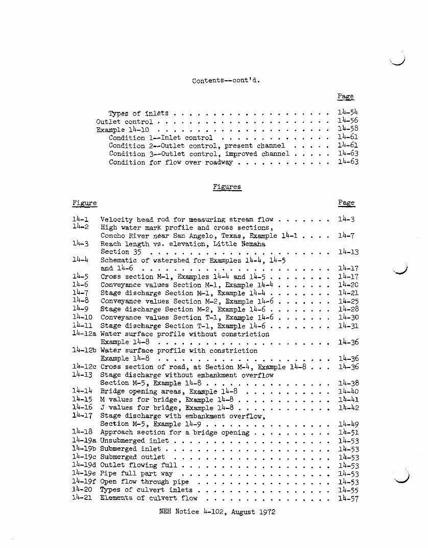
. . . . . . . 14-1 Velocity head rod for measuring stream flow 14-2 High water mark prof i le and cross sections. . . . . Concho River near San Angelo. Texas. Example 14-1 14-3 Reach length vs . elevation. L i t t l e Nemaha
Section 35 . . . . . . . . . . . . . . . . . . . . . . . 14-4 Schematic of watershed f o r Examples 14.4. 14-5 . . . . . . . . . . . . . . . . . . . . . . . . and14-6 . . . . . . . . 14-5 Cross section M.1. Examples 14-4 and 14-5 . . . . . . . 14-6 Conveyance values Section M.1. Example 14-4 . . . . . . . . 14-7 Stage discharge Section M.1. Example 14-4 . . . . . . . 14-8 Conveyance values Section M.2. Example 14-6
. . . . . . . . 14-9 Stage discharge Section M.2. Example 14-6 . . . . . . . 14-10 Conveyance values Section T.1. Example 14-6
. . . . . . . . 14-11 Stage discharge Section T.1. Example 14-6 14-12a Water surface prof i le without constriction
Example 14-8 . . . . . . . . . . . . . . . . . . . . . . 1 4 - 1 2 Water surface prof i le with constrict ion
Example 14-8 . . . . . . . . . . . . . . . . . . . . . . . . . 14-12c Cross section of road. a t Section ~ . 4 . Example 14-8 14-13 Stage discharge without embankment overflow
Section M.5. ExarnpLe 14-8 . . . . . . . . . . . . . . . . 14-14 Bridge opening areas. Example 14-8 . . . . . . . . . . . 14-15 M values fo r bridge. Example 14-8 . . . . . . . . . . . . 14-16 J values f o r bridge. Example 14-8 . . . . . . . . . . . . 14-17 Stage discharge with embankment overflow.
Section M.5. Example 14-9 . . . . . . . . . . . . . . . . 14-18 Approach section for a bridge opening . . . . . . . . . . 14-19a Unsubmerged i n l e t . . . . . . . . . . . . . . . . . . . . 14.191, Submerged i n l e t . . . . . . . . . . . . . . . . . . . . . 14-19c Submerged out le t . . . . . . . . . . . . . . . . . . . . 14-19d Outlet flowing full . . . . . . . . . . . . . . . . . . . 14-19e Pipe f u l l par t way . . . . . . . . . . . . . . . . . . . 14-19f Open flow through pipe . . . . . . . . . . . . . . . . . 14-20 Types of culvert i n l e t s . . . . . . . . . . . . . . . . . 14-21 Elements of culvert flow . . . . . . . . . . . . . . . .
NEH Notice 4.102. August 1972

Figure
14-22a Cross section T-3 . . ., . . . . . . . . . . . . . . . . . . 14-22b =ofile through culvert, Example 14-10 . . . . . . . . . . 14-23 Stage discharge exit Section T-2,
Example 14-10 . . . . . . . . . . . . . . . . . . . . . . . 14-24a Rating curves cross section T-4, assuming
no roadway in place, Example 14-10 . . . . . . . . . . . . 14-24b Rating curves cross section T-4, inlet
control,. Example 14-10 . . . . . . . . . . . . . . . . . . 14-24c Rating curves cross section T-4, outlet control,
Example 14-10 . . . . . . . . . . . . . . . . . . . . . . . 14-24d Rating curves cross section T-4, improved
channel-outlet control, Example 14-10 . . . . . . . . . . . Tables
Table - 4 Computation of discharge using Velocity
<\/, Head Rod (VHR) measurements . . . . . . . . . . . . . . . . 14-2a Data for computing discharge from modified
slope-area measurements; cross section A at station 4+20. Example 14-1 . . . . . . . . . . , . . . .
14-3 Hydraulic parameters for cross section M-1, Example 14-4 . . . . . . . . . . . . . . . . . . . . . . . .
14-4 Stage discharge for Section M-1 with meander correction, Example 14-5 . . . . . . . . . . . . . .
14-5a Water surface profiles from cross section M-1 to M-2, Example 14-6 . . . . . . . . . . . . . . . . . . . .
14-6 Back water computations through bridges, Example 14-8 . . . 14-7 Stage discharge over roadway at cross section
M-4, without submergence, Example 14-9 . . . . . . . . . . . 14-8 Headwater computations for eight 16' x 8'
concrete box culverts, headwalls parallel to embankment (no wingwalls) square edged on three sides, Example 14-10 . . . . . . . . . . . . . . . . . . . .
14-9 Stage discharge over roadway at cross section T-3, Figure 14-4, Example 14-10 . . . . . . . . . . . . . . . . .
Exhibits
Exhibit
L 14-1 K values for converting CSM to CFS . . . . . . . . . . . . . 14-67 14-2 Estimate of head loss in bridges . . . . . . . . . . . . . . 14-68 14-3 Estimate of M for use in BPR equation . . . . . . . . . . . 14-69 14-4 BPR base curve for bridges (K~). . . . . . . . . . . . . . . 14-70
NEH Notice 4-102, August 1972

Ekhibits--cont 'd .
Exhibit
14-5 Incremental backwater coeff ic ient f o r the more . . . . . . . common types of columns, p i e r s and p i l e bents 14-6 Headwater depth f o r box cu lve r t s with i n l e t
control . . . . . . . . . . . . . . . . . . . . . . . . . . 14-7 Headwater depth f o r concrete pipe culver ts with
i n l e t c o n t r o l . . . . . . . . . . . . . . . . . . . . . . . 14-8 Headwater depth f o r oval concrete pipe
culver ts long axis hor izonta l with i n l e t con t ro l . . . . . 14-9 Headwater depth f o r C. M. pipe cu lve r t s
with i n l e t control . . . . . . . . . . . . . . . . . . . . 14-10 Headwater depth f o r C. M. pipe-arch cu lve r t s
with i n l e t control . . . . . . . . . . . . . . . . . . . . 14-11 Head f o r concrete box culver ts flowing f u l l
n = 0 . 0 1 2 . . . . . . . . . . . . . . . . . . . . . . . . . 14-12 Head f o r concrete pipe cu lve r t s flowing f u l l
n = 0 . 0 1 2 . . . . . . . . . . . . . . . . . . . . . . . . . 14-13 Head f o r oval concrete pipe culver ts long a x i s
hor izonta l or v e r t i c a l flowing f u l l n.= 0.012 . . . . . . . 14-14 Head f o r standard C. M. p ipe culver ts flowing
full n = 0.024 . . . . . . . . . . . . . . . . . . . . . . 14-15 Head f o r standard C. M. pipe-arch culver ts
flowing ful l n = 0.024 . . . . . . . . . . . . . . . . . . 14-16 C r i t i c a l depths-rectangular sec t ion . . . . . . . . . . . . 14-17 C r i t i c a l depth. Circular pipe . . . . . . . . . . . . . . 14-18 C r i t i c a l depth. Oval concrete pipe. Long
ax i s hor izonta l . . . . . . . . . . . . . . . . . . . . . . 14-19 C r i t i c a l depth. Standard C. M. pipe-arch . . . . . . . . . 14-20 C r i t i c a l depth. S t r u c t u r a l p la te . C. M. pipe-
axch . . . . . . . . . . . . . . . . . . . . . . . . . . . 14-21 Entrance l o s s coeff ic ients . . . . . . . . . . . . . . . .
NM Notice 4-102, August 1972

NATIONAL ENGINEERING HANDBOOK
SECTION 4
HYDROLOGY
CHAPTER 14 . STAGE DISCMGE RELATIONS
Introduction
In planning and evaluating the s t ruc tura l measures of watershed protec- t ion , it i s necessary for SCS engineers and hydrologists t o develop stage discharge curves a t selected locations on natural streams.
Many hydraulics textbooks and handbooks, as well as NM-5, contain methods for developing stage discharge curves assuming non-uniform steady flow. Some of these methods are elaborate and time consuming. The type of available f i e l d data and the use t o be made of these stage discharge curves should d ic ta te the method used i n developing the curve.
This chapter presents a l ternate methods of developing these curves a t selected points on a natural stream.
Manning's formula has been used t o develop stage discharge curves for natural streams assuming the water surface t o be pa ra l l e l t o the slope of the channel bottom. This can lead t o large e r rors , since t h i s condition can only ex is t i n long reaches having the same bed slope with- out a change i n cross section shape or retardance.
This condition does not ex i s t i n naturaZ streams.
The r a t e of change of discharge for a given portion of the stage dis- charge curves d i f fe rs between the r i s ing and f a l l i ng s ides of a hydrograph. Some streams occupy re la t ive ly small channels during low flows, but overflow onto wide flood plains during high discharges. On the r i s ing stage the flow away from the stream causes a steeper slope than tha t f o r a constant discharge and produces a highly variable discharge with dis- tance along the channel. After passage of the flood c r e s t , the water re-enters the stream and again causes an unsteady flow, together with a stream slope l e s s than tha t for a constant discharge. The effect on the stage-disch ge re la t ion i s t o produce what i s cal led a loop ra t ing for each flood.? Generally i n the work performed by the SCS t he maximum stage the water reached i s of primary in te res t . Therefore, the stage dis- charge curve used for routing purposes is a p lo t for t h e maximum elevation obtained during the passage of flood hydrographs of varying magnitudes. This r e su l t s i n the plot being a single l i ne .
Handbook of Applied Hydrology, Ven Te Chow, page 15-37.
NEH Notice 4-102, August 1972
Development of Stage Dischar~e Curves
Direct Measurement
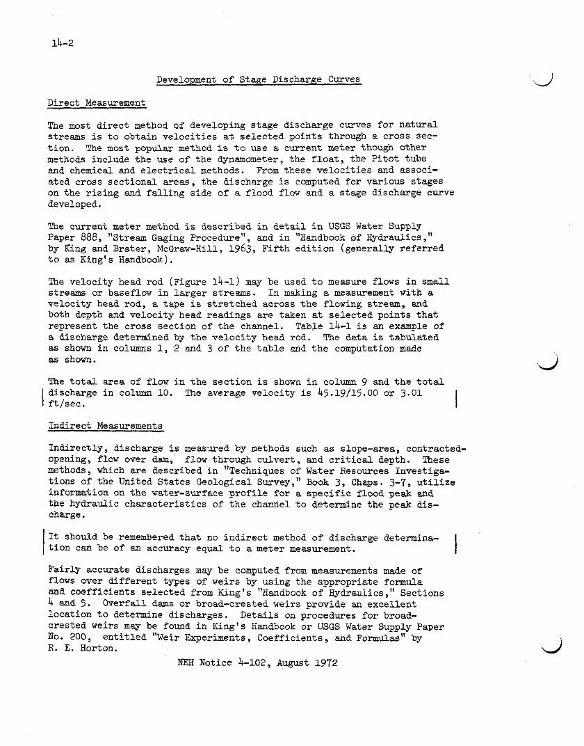
The most direct method of developing stage discharge curves for natural streams i s t o obtain veloci t ies a t selected points through a cross sec- t ion. The most popular method i s t o use a current meter though other methods include the use of the dynamometer, the f l o a t , the P i to t tube and chemical and e l ec t r i ca l methods. From these veloci t ies and associ- ated cross sectional areas, the discharge i s camputed for various stages on the r i s ing and f a l l i ng side of a flood flow and a stage discharge curve developed.
The current meter method i s described i n d e t a i l i n USGS Water Supply Paper 888, "Stream Gaging Procedure", and i n "Handbook of Hydraulics," by King and Brater, McGraw-Hill, 1963, F i f th edi t ion (generally referred t o as King' s Handbook).
The velocity head rod ( ~ i g y r e 14-1 ) may be used t o measure flows i n small streams or baseflow i n la rger streams. I n making a measurement with a velocity head rod, a tape i s s t re tched across t he flowing stream, and both depth and velocity head readings are taken a t selected points t ha t represent the cross section of t he channel. Table 14-1 i s an example of a discharge determined by the veloci ty head rod. The data i s tabulated as shown i n columns 1, 2 and 3 of the tab le and the computation made as shown.
The t o t a l area of flow i n the sect ion is shown i n column 9 and t he t o t a l
I discharge i n column 10. The average velocity is 45.19/15.,00 or 3.01 f t /sec . I Indirect Measurements
Indirectly, discharge i s measured by methods such as slope-area, contracted- opening, flow over dam, flow through culvert , and c r i t i c a l depth. These methods, which are described i n "Techniques of Water Resources Investiga- t ions of the United States Geological Survey," Book 3, Chaps. 3-7, u t i l i z e information on the water-surface p ro f i l e for a spec i f ic flood peak and the hydraulic character is t ics of the channel t o determine the peak dis- charge.
It should be remembered t h a t no ind i rec t method of discharge determina- t ion can be of an accuracy equal t o a meter measurement. I Fairly accurate discharges may be computed from measurements made of flows over different types of weirs by using the appropriate formula and coefficients selected from King's "Handbook of Hydraulics," Sections 4 and 5. Overfall dams or broad-crested weirs provide an excellent location t o determine discharges. Details on procedures for broad- crested weirs may be found i n King's Handbook o r USGS Water Supply Paper No. 200, en t i t l ed "Weir Experiments, Coefficients, and Formulas" by R. E. Horton.
NEH Notice 4-102, August 1972

The r o d i s f i r s t p l a c e d i n t h e w a t e r w i t h i t s f o o t on t h e bottom and t h e s h a r p e d g e f a c i n g d i r e c t l y up- s t ream. The s t r e a m d e p t h a t t h i s p o i n t is i n d i c a t e d by t h e w a t e r e l e v a t i o n a t t h e s h a r p edee , n e g l e c t i n g t h e s l i g h t r i p p l e o r bow wave. I f t h e rod is now re - v o l v e d 180 d e g r e e s , s o t h a t t h e f l a t edge is t u - n e d u p s t r e a m a h y d r a u l i c jump w i l l b e f o r m e d b y t h e o b s t r u c t i o n t o t h e f l o w o f t h e s t r e a m . Af te r t h e d e p t h or f i r s t r e a d i n g h a s been s u b t r a c t e d from t h e second r e a d i n g , t h e n e t h e i g h t o f t h e jump e q u a l s t h e a c t u a l v e l o c i t y h e a d a t t h a t p o i n t . V e l o c i t y c a n t h e n be computed by t h e s t a n d a r d formula,
v = J 2 g h = 8.02 Ji; A i n which v = V e l o c i t y i n f t . p e r s e c .
g = A c c e l e r a t i o n u f g r a v i t y (32.16 f t . p e r
d" Brass See
Cuttrng Edge
SECTION B 8
V E L O C I T Y H E A D ROD Developed a t San Di re r
E x ~ e r l r e n t a l Fores t
sec. p e r s e c . h ' V e l o c i t y head, i n f t .
The a v e r a g e d i s c h a r g e f o r t h e s t r e a m i s ob ta ined by t a k i n g a number o f measurements o f d e p t h and v e l o c i t y t h r o u g h o u t i t s c r o s s s e c t i o n . Q = AV. i n which Q = d i s c h a r g e c f s : A = c r o s s s e c t i o n a l a r e a , s q . f t . V = v e l o c i t y , f t . p e r sec .
V E L O C I T Y F O R D I F F E R E N T VALUES O F " h a v - 8.02 6
h, Velocity Head in Pt.
-05 .lo el5 .P -25 .X, -35 .40 4 5 .50
Figure 14-1. V e l o c i t y head r o d for measuring s t r e a m flow.
NEE N o t i c e 4-102, August 1972
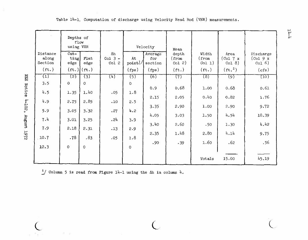
Table 14-1. Computation of discharge using Velocity Head Rod (VHR) measurements.
Distance along
Section
(ft.)
-r 3.5
4.5
4.9
5.9
7.4
7.9
10.7
12.3
Depths of flow
using VHR
ting Flat I Ah Col 3 - COl 2
(4)
-05
.10
27
.24
-13
.O5
'/ Collumn 5 is read from Figure 14-1 using the Ah in column 4. -
Width (from Col 1)
(ft.)
(8)
1.00
0.40
1.00
1.50
.50
2.80
1.60
Totals
Area (Col 7 x Col 8)
(ft.2)
(9)
0.68
0.82
2.90
4.54
1.30
4.14
.62
- 15.00
Discharge (Col 9 x C O ~ 6)
(cfs)
(10)
0.61
1.76
9.72
18.39
4.42
9.75
.56
- 45.19

Slope-Area Estimates Field measurements taken a f te r a flood are used t o determine one or more points on the stage-discharge curve a t a selected location. The peak discharge of the flood i s estimated using high water marks t o determine the slope.
Three or four cross sections are usually surveyed so t h a t two o r more independent estimates of discharge, based on pairs of cross sections, can be made and averaged. Additional f i e l d work required for slope- area estimates consists of selecting the stream reach, estimating "n" values and surveying the channel p rof i le and high water p rof i le a t selected cross sections. The work i s guided by the following:
1. The selected reach i s as uniform i n channel alignment, slope, s i ze and shape of cross section, and factors affecting the roughness coefficient "n" as i s practicable t o obtain. The selected reach should not contain sudden breaks i n channel bottom wade, such as shallow drops - . or rock ledges.
2. Elevations of selected high water marks are determined on both ends of each cross section.
3. The three or more cross sections are located t o represent as closely as possible the hydraulic character is t ics of t he reach. Dis- tances between sections must be long enough t o keep small the errors i n estimating stage or elevation.
The flow i n a channel reach is computed by one of the open-channel for- mulas. The most commonly used formula i n the slope area method i s the Manning equation
Where Q i s the discharge, n i s the coefficient of roughness, A i s the cross sectional area, R i s the hydraulic radius, and S i s the slope of the energy gradient. Rearranging Eq. 14-1 gives
The r igh t side of Eq. 14-2 contains only the physical character is t ics of the cross section and i s referred t o as the conveyance fac tor Kd. The slope i s determined from the elevations of t he highwater mark and the distances between the high water marks along the direct ion of flow.
Modified Slope Area Method The following equations based on Bernoulli 's theorem a re discussed f'ully i n NM-5, Supplement A.
(Eq. 14-31
NEH Notice 4-102, August 1972

14-6
where q = discharge, i n cfs El = elevation of the water surface a t the upstream section
- elevation of the water surface a t the downstream section and Ui = symbols used by Doubt for cer ta in computed values;
(See NEH-5, p q e A.14 )
The working eauation i s derived from eauation 14-1.
Also from MER-j -
and:
where 9, i s the length of the reach between sections 1 and 2, and the other symbols are as defined i n NM-5. The noaographs shown i n NM-5, Supplement A as standard drawings ES-75, 76, and 77 are expedient work- ing tools used t o solve Equations 14-4, 14-5 and 14-6.
The following example i l l u s t r a t e s the modified slope area method and the use of Eq. 14-2. The example i s based on data taken from USGS Water Supply Paper 816 ( ~ a j o r Texas Floods of 1936).
Example 14-1 - Using data f o r the Concho River near San Angelo, Texas, for the September 17, 1936, flood compute the peak discharge t h a t occurred. Figure 14-2 shows Section A and B with the high water mark p ro f i l e d o n g the stream reach between the two sections.
1. Draw a water surface t h r o u ~ h the average of the high water w. From Figure 14-2 the elevation of the water surface a t the lower cross section B is 55.98 designated i n t he example as Ez. The elevation of t he water surface a t cross section A i s 56.50 designated as E l .
2. Compute the length of reach between t h e two sections. From Figure 14-2 the length of reach i s 680 fee t .
3. Divide each cross section i n t o sements as needed due t o different "n" values as shown i n Figure 14-2.
In computing the hydraulic parameters of a cross sect ion on a natural stream when flood plain flow ex i s t s , it is desirable t o divide the cross section in to segments. The number of seg- ments w i l l depend on the i r regular i ty of the cross section and
NEH Notice 4-102, Augus t 1972

Sscllon A
30 -
20 -
lo - Section B
I I I I , I I 1 I I I I I I I I I I I I 4 2 t O O 4 + 0 0 6 + 0 0 W O O lO+OO 12+00 1 4 t O O 16+00 1 8 t O O 2 0 + 0 0 2 2 W O
STATIONS
Figure 14-2. High water mark profile and cross sections, Concho River near San Angelo, Texas. Example 14-1.
I-'
f- 4

the variation i n "n" values assigned t o the different portions. II ,t NEH-5, supplement B, gives a method of determining n values
for use i n computing stage discharge curves.
4. Compute the cross sect ional area and wetted perimeter f o r each segment of each cross section. Tabulate i n columns 2 and 3 of Table 14-2(a) for cross section A and Table 14-2(b) for cross section B.
5. Compute F = 1.486 A R ~ / ~ fo r each segment. Using standard drawing ES-76 (NM-5), compute F and tabulate i n column 4, Table 14-2(a) and 14-2(b).
6. Compute Q/s'/' = 1.486 A R ' / ~ . Tabulate the "n" value assigned
t o each segment i n column 5 of Table 14-2(a) and 14-2(b). Col- umn 6 i s ~ / s ' / ~ a n d i s computed by dividing column 4 by column 5 or by using ES-77 (NEE-5). This i s commonly called the flow fac tor of conveyance and i s generally designated as Kd.
7. Compute the t o t a l area and the t o t a l Kd. Sun columns 2 and 6 of Table 14-2(a) and 14-2(b).
8. Compute U. Using Eq. 14-6 or ES-77 compute U- for the down- stream cross section A using data from Table 14-2(a).
From Eq. 14-6: U- = 1. - a a: q:
9 . Compute U+ Using Eq. 14-5 or ES-77 compute $ for upstream cross section B using data i n Table 14-2(b).
. NEH Notice 4-102, August 1972

Table 14-248) Data for computing discharge f r om modified slope-area measurements; Cross Section A a t Station 4+20. &le 14-1
Area - (2)
2354
12691
5862
5385
2523
2498
3416 - 34729
Wetted Perimeter
Table 14-2b) Data for computing discharge from modified slope-area rur-te; Cross Section B a t Station U+100. &smple 14-1
Wetted Perimeter F I n Begment
(3 ' 1
2
3 4
5 6 7 8
(210-VI-NEH-4, Amend. 6 , March 1985)
Area
(2)
1598 11750
4750
2486 4944
3455 2270
1518 - 32771

= (680) (32.2) (1.32 x lo-") = 2.89 x lo-'"
U+ = (9.31 x 10"' + 2.89 x lo-' ') = 12.20 x lo-''
l o . Compute q. Using Eq. 14-4. p = 28 ( E ~ - EZ. )) '/' IJ$ - U i
Fb = 2) (32.2) (56.50 - 55-98} = los bi (12.20 - 5.71) x lo-'' P':
q = 2.265 x l o 5 or q = 226,500. This compares with the discharge of 230,000 cfs computed by USGS i n Water Supply Paper 816.
Synthetic methods There are various methods which depend en t i re ly on data which may be gathered a t any time. These methods es tabl ish a water surface slope based ent i re ly on the physical elements present such as channel s i ze and shape, flood plain s i ze and shape and the roughness coeff ic ient . The method generally used by the SCS is the modified s tep method.
This method bases the r a t e of f r i c t i on loss i n the reach on t h e elements of the upstream cross section. Manning's equation is applied t o these elements and the difference i n elevation of the water surface plus t h e difference i n velocity head between the two cross sections is assumed t o be equal t o the t o t a l energy loss i n the reach. This method, ignor- ing t h e changes i n velocity head, i s i l l u s t r a t ed i n Example 14-6.
Selecting Reach Lengths
The flow distance between one section and the next has an important bearing on the f r ic t ion losses between sections. For flows which a re ent i re ly within the channel the channel distance should be used. On a meandering stream the overbank portion of the flow may have a flow dis- tance less than the channel distance. This distance approaches but does not equal the floodplain distance due t o the e f fec t of the channel on the flow.
From a pract ical standpoint the water surface i s considered leve l across a cross section. Thus the elevation difference between two cross sections i s considered equal for both the channel flow portion and the overbauk portion.
It has been common pract ice t o compute the conveyance for t h e t o t a l sec- t ion then compute the discharge by using a given slope with t h i s convey- ance, where the channel portion by the formula:
slope used is-an average slope between the slope of t he and the overbank portion. The average slope i s computed
NW Notice 4-102, August 1972

where: Sa = average slope of energy gradient i n reach H = elevation difference of the energy leve l between sections La = average reach length
The reach length La can be computed as follows:
where qc = discharge i n channel portion Kdc = conveyance i n channel portion Sc = energy gradient in channel portion qf = discharge i n floodplain portion Kdf = conveyance i n floodplain portion Sf = energy gradient i n floodplain portion q t = t o t a l discharge Kdt = t o t a l conveyance Sa = average slope of energy gradient
The t o t a l discharge i n a reach i s equal t o the flow i n channel plus the flow i n the overbank.
Substi tuting from Equations 14-8, 14-9 and 14-10
Kdt x sal/' = KdC x sC1/* + Kdf x (Eq. 14-12)
H Let S = -. L
where H = elev. of reach head - elev. of reach foot L = length of reach
Then subst i tut ing in to Eq. 14-12 using the proper subscripts
Divide both sides by HI/'
If -the average reach length i s plot ted vs. elevation f o r a section then it i s possible t o read the reach length direct ly t o use with the Kd for any desired elevation. The data w i l l p lo t i n a form as shown i n Figure 14-3.
mM Notice 4-102, August 1972
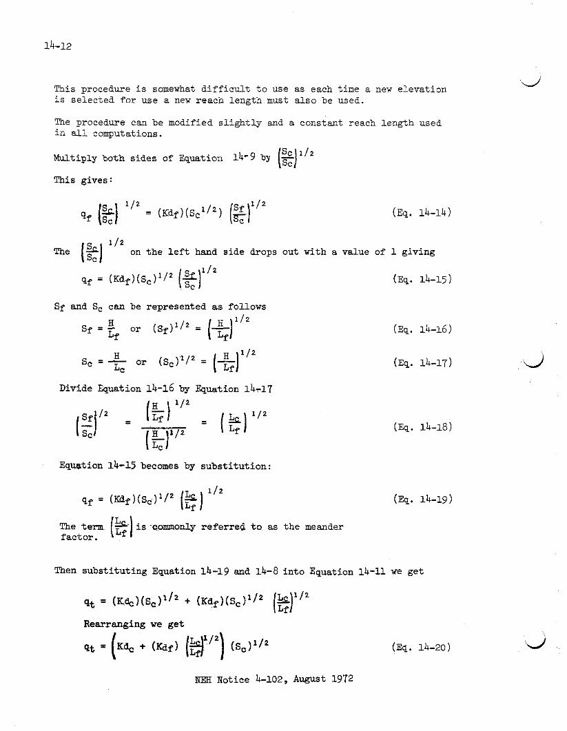
This procedure is somewhat difficult to use as each time a new elevation is selected for use a new reach length must also be used.
The procedure can be modified slightly and a constant reach length used in all computations.
Multiply both sides of Equation 14-9 by
This gives:
1 /' on the left hand side drops out with a value of 1 giving
Sf and S, can be represented as follows
Divide Equation 14-16 by Equation 14-17
Equation 14-15 becomes by substitution:
(Eq. 14-19)
The term ($1 is commonly referred to as the meander factor.
Then substituting Equation 14-19 and 14-8 into Equation 14-11 we get
Rearranging we get
NEH Notice 4-102, August 1972

1m
1015 I
1010
r 1005 E l- a z = Iwo
995
MEANDE
990
985 3600 3am 4
Figure 14-3. Reach length vs. e l eva t ion , L i t t l e Nemaha Section 35.

Equation 14-20 can be used t o compute the t o t a l stage discharge a t a section by using the channel reach length ra ther than a variable reach length. Example 14-5 i l l u s t r a t e s the use of modifying the flood plain conveyance by the square root of the meander factor i n developing a stage discharge curve.
Discharge vs. Drainage Area
It is desirable for the water surface prof i le t o represent a flow which has the same occurrence interval throughout the watershed. The CSM (cubic fee t per second per square mile) values for most floods vary within a channel system having a smaller value for l a rger drainage areas. Thus when running a prof i le the 50 CSM of the ou t le t , the ac tua l CSM r a t e w i l l increase as the prof i le progresses up the watershed.
The r a t e of discharge a t any point i n the watershed i s based on the f o r m ~ l a i f
where Q is discharge i n CSM A is the drainage area
and C is a coefficient depending on the character is t ics of the watershed
Assuming tha t C remains constant f o r any point i n the watershed, then the discharge at any point i n the watershed may be re la ted t o the dis- charge of any other point i n the watershed by the formula
where Q1 and A1 represent the discharge r a t e i n CSM and drainage area of one point i n the watershed and Q2 and AZ represent the CSM and drain- age area a t another.
In practice Qz and AZ usually represent the ou t le t of the watershed and remain constant and A1 i s varied t o obtain Q1 a t other points of i n t e r e s t .
Equation 14-22 i s plot ted i n Exhibit 14-1 f o r the case where A2 is 400 square miles. This curve may be used d i rec t ly t o obtain the CSM
-
A' Engineering For D m , Vol. 3 page 125, Creager , Jus t in & Hines .
NEH Notice 4-102, August 1972

discharge of the ou t le t if the ou t le t i s a t 400 square miles as shown in Example 14-2. Example 14-3 shows how t o use Exhibit 14-1 if the drain- age area at the out le t i s not 400 square miles.
Example 14-2
Find the CSM value t o be used for a reach with a drainage area of 50 square miles when the CSM a t the ou t le t i s 80 CSM. The drainage area at the out le t i s 400 square miles.
1. Determine K f o r a drainage area of 50 sauare miles. From Exhibit 14- lwi th a drainage area of 50 square miles read K = 2.61.
2. Determine CSM r a t e f o r 50 sauare miles. Multiply CSM a t t he ou t le t by K computed i n s t ep 1.
Example 14-3
Find the CSM r a t e t o be used at a reach with a drainage area of 20 squme miles if the drainage area a t the out le t i s 50 square miles. !The CSM r a t e a t the ou t le t is 60 CSM.
1.. Determine K f o r a drainage area of 20 sauare miles. From Exhibit 14-1 f o r a drainage area of 20 square miles read K = 3.66.
2. Determine K f o r a drainage area of 50 sauare miles. From Exhibit 14-1 for a drainage area of 50 square miles read K = 2.61.
3. Compute a new K value for a drainage area of 20 square
miles. Divide s tep 1 by s t ep 2.
4. Determine CSM r a t e f o r the 20 sauare mile drainage area. Multiply K obtained i n s tep 3 by the CSM a t the out le t .
Computing Prof i les
When using water surface prof i les t o develop stage discharge curves for flows a t Paore than c r i t i c a l depth, it is necessary t o have a stage dis- 1 charge curve for a s t a r t i ng point a t t he lower end of a reach. This s ta r t ing point may be a stage discharge curve developed by current meter measurements or one computed from a control section where the flow passes through c r i t i c a l discharge; o r it may be one computed from the elements
(210-VI-NEH-4, Amend. 6, March 1985)

of the cross section and an estimate of t he slope. The l a t t e r case i s the most commonly used by SCS since the more accurate stage discharge curves are not generally avai lable on small watersheds. I n most cases it i s advisable t o locate three o r four cross sections close together i n order t o eliminate par t of t he error i n estimating the slope used i n developing the stage discharge c w e a t the lower or f i r s t cross sec- t ion on a watershed.
Example 14-4
Develop the s t a r t i ng stage discharge curve for cross section M-1 (Figure 14-4) shown as the f i r s t cross section a t t he out le t end of the water- shed, assuming an energy gradient of .001 f t / f t .
1. Plot the surveyed cross section. From f i e l d survey notes, p lo t the cross section, Figure 14-5(a) noting the points where there i s an apparent change i n the "nu value.
2 . Divide the cross section into segments. An abrupt change i n shape or a change i n "n" i s the main factor t o be considered i n determining extent and number of segments required for a par- t i c u l a r cross section. Compute $he "n" value f o r each segment using NM-5, Supplement B, or the "n" may be based on other data or publications.
3. Plot the channel segment on an enlarged scale. Figure 14-5(b), for use i n computing the area and measuring the wetted peri- meter a t selected elevations i n t he channel. The length of the segment a t selected elevations i s used as t he wetted perimeter for the flood plain segments. The division l i n e between each segment i s not considered as wetted perimeter.
4. Tabulate elevations t o be used i n making computations. Star t ing a t an elevation equal t o or above any flood of record, tabulate i n column 1 of able 14-3 the elevations tha t w i l l be- required t o define the hydraulic elements of each segment.
5. Compute the wetted perimeter a t each elevation l i s t e d i n s tep 4. Using an engineer's scale and s t a r t i ng a t the lowest elevation i n column 1, measure the wetted perimeter of each segment a t each elevation and tabulate i n columns 3, 7, 11, and 15 of Table 14-3. Note t ha t t he maximum wetted perimeter for the channel segment i s 62 at elevation 94.
6. Compute the cross sect ional area fo r each elevation l i s t e d i n step 4. S ta r t ing a t t he lowest elevation, compute the accumu- la ted cross sectional area for each segment a t each elevation i n column 1 and tabulate i n columns 2, 6, 10, and 1 4 of Table 14-3.
7. Compute F factor . F = 1 . 4 8 6 ~ ~ ~ ' ~ f o r each elevation. Using standard drawing ES-76, compute t h e F factor f o r each segment
NEE Notice 4-102, August 1972

Figure 14-4. Schematic of Watershed for Examples 14-4, 14-5, and 14-6.
NEH Notice 4-102, August 1972

NEH Notice 4-102, August 1972

Table 14-3. Wdraulic parameters for starting crdss section M-1, Example 14-4.
- US" - (1)
LO5
102
LOO
98
96
99
94
93
91
89
81
85
82
- l h o solve this on E8-I1 divide P by 2, then double rssulta read from Sheet 3. P6-11, 5l1o order t e eolve thia on E8-I6 it La necossacy t o divide both area and W by 2 aai
meat 3
*dlg,b
(13)
2.38 x 10:
1.82 r lo!
1.48 x 10:
1.11 x 10:
8.9 x10 '
7.6 r LO'
6.4 x lo'
5.61 r lo'
3.92 x 10'
2.51 r 10'
1.40 x 10'
5.90 x lo!
0
t 4 - Wso*
(11)
2.49 x 10'
1.44 x lo '
9.06 1 lo!
4.60 x lo!
1.56 x 10:
5.78 10'
6.32 1 10:
0
I then double the P factor read from Bbeet 3, -16.
NOTE: q,,dl~o* i s the ssms a. Kd or ca-oly referred t o as the convey(U1ee factor.
NEH Notice 4-102, August 1972

N O l l V A 3 1 3
NEH Notice 4-102, August 1972

a t each elevation i n column 1 and tabulate i n columns 4 , 8, 12, and 16 , Table 14-3.
8. Compute the conveyance factor bd /~01 /2 for each elevation.
Using standard drawing ES-77 and the assigned "n" value for each segment compute k d for each segment a t each eleva- t i on i n column 1 and tabulate i n columns 5, 9 , 13, and 17 of Table 14-3. This can a l so be done by dividing F by n using a s l ide ru le or desk calculator.
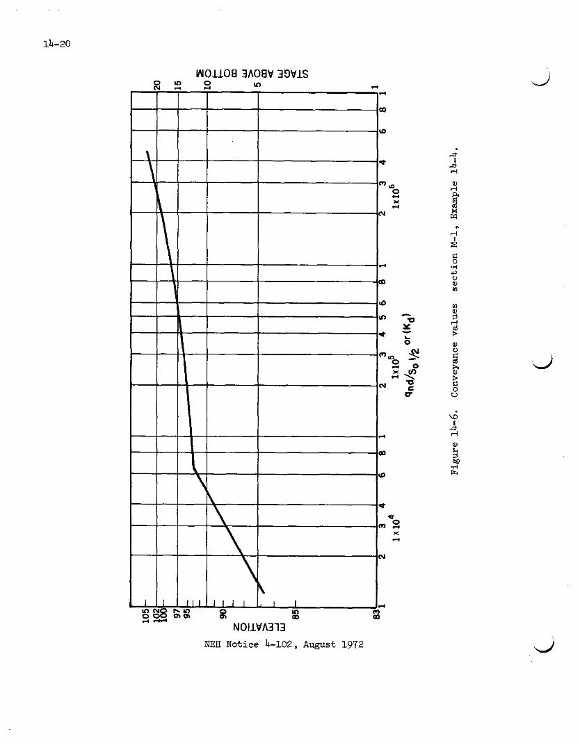
9 . Sum columns 5, 9, 13, and 1 7 and tabulate i n column 18. A plot of column 18 on log-log paper i s shown on Figure 14-6. 'Ke elevation scale i s selected based on f ee t above the channel bottom.
10. Compute the d i s c h a r ~ e for each elevation. Using the average slope a t cross section M-1, S = .001, develop stage discharge for cross section M-1, q = s'l2 x qnd /~01 /2 , or q = s'/' x Kd. The stage discharge curve f o r cross section M-1 i s shown on Figure 14-7.
The next example shows the e f fec t of a meandering channel i n a flood- plain on the elevation discharge relationship. Equation 14-20 w i l l be used t o determine the discharge.
Example 14-5
Develop the stage discharge curve for cross sect ion M-1 ( ~ i g u r e 14-4) if M-1 represents a reach having a c h n n e l length of 2700 feet and a floodplain length of 2000 f ee t . The energy gradient of the channel por- t ion i s 0.001 ft./ft.
1. Compute the t o t a l floodplain conveyance Kdf.
Figure 14-5 shows segments 1, 2 and 4 of section M-1 a re floodplain segments. Table 14-3 of Example 14-4 was used t o develop the hydraulic parameters for sect 'on M-1 for each
1 7 2 segment. From Table 14-3 add the &nd/So values for each elevation from columns 5 , 9, and 17 and tabulate as Kdf i n column 2 of Table 14-4.
2. Determine the meander factor L c / ~ f . For the channel length
of 2700 fee t and the floodplain length of 2000 feet the meander factor i s :
3. Determine Lc/Lf 1 / 2 .
NEH Notice 4-102, August 1972

Table 14-4. Stage discharge f o r Section M-1 w i th meander correct ion, Example 14-5
Levat ion Floodplain
Kdf
( 2 )
4.54 x l o 6
2.64 X l o 6
1.64 x l o 6
8.30 X 10'
2.72 X 10'
9.55 x 10'
6.99 x 1 0 3
0.
0.
Channel
Kdc
(4)
2.38 X l o 5
1.82 X 10'
1.48 x 10⁵
1.17 X 10'
8.9 X 10"
7.6 x 10'
6.4 X 10"
5.61 x l o '
3.92 X 10"
Col. 3 + Col. 4
( 5 )
5.51 X l o 6
3.24 X l o 6
2.05 X l o 6
1.08 'x l o 6
4.05 x 1 0 5
1.87 X l o 5
7.21 X 10'
5.61 x l o 4
3.92 X l o 4
Discharge Qt
(61
174000
102000
64800
34100
12800
5910
2280
1170
1240

Compute ( ~ d f ) (LC/L~) ' / ' . For each elevation i n column 1 of
Table -14-4 multiply column 2 by ( L ~ / L ~ ~ l / ~ a n d tabulate i n col- umn 3.
(4.54 x l o 6 ) (1.16) = 5.27 x l o 6
Compute the channel conveyance Kd. From Figure 14-4 the chan- nel i s segment 3 and the conveyance has been calculated i n col- umn 13 of Table 14-3. Tabulate Kdc i n column 4 of Table 14-4.
Compute Kdc + (Kdf ) (LC/L*) I/ '. From Table 14-4 add columns
3 and 4 and tabulate i n column 5.
Compute the discharge f o r each elevation. Use Sc = .001 and Equation 14-20. Multiply columns by ~ , l / ' and tabulate i n column 6.
The next example w i l l show the use of the modified step method i n comput- ing water surface prof i les . It i s a t r i a l and e r ror procedure based on estimating the elevation a t the upstream section, determi ing the con-
1 1 2 veyance, Kd, for the estimated elevation and computing S by using
Mannings equation i n the form S 1.486 AR2/3. is = 9 where Kd % - Kd n --
the head loss per foot (neglecting velocity head) from the downstream t o t h e upstream section. 'Ihis head loss added t o the downstream water surface elevation should equal the estimated upstream elevation.
Example 14-6
Using the r a t i ng curve developed i n Example 14-4 f o r cross section M-1 and parameters plot ted on Figures 14-8 and 14-10 f o r cross sections M-2 and T-1, compute the water surface prof i les required t o develop stage discharge curves for cross sections M-2 and T-1. The changes i n veloci ty head w i l l be ignored f o r these computations. The drainage area at section M-1 i s 400 sq. m i . , a t M-2 i s 398 sq. m i . and a t T-1 i s 48 sq. mi. The reach length between M-1 and M-2 is 2150 f ee t and between M-2 and T-1 i s l l50 fee t . Assume the meander fac tor for t h i s example i s 1.0.
1. Determine the range of csm needed t o define the stage discharge curve. One or more of the csm's selected should be contained - within the channel. Tabulate i n column I, Table 1 4 - ~ ( a ) .
2. Compute the discharge i n cfs for each csm a t the two cross sec- t ions M-1 and M-2. A t section M - 1 the drainage area i s 400 sq. m i . Using Exhibit 14-1 the K factor i s 1.0 and the cfs for 2 csm i s 2 x 400 x 1.0 = 800 cfs . A t section M-2 the drainage
NM Notice 4-102, August 1972

NEH Notice 4-102, August 1972

Table 14-5(a). Water Surface prof i les from cross section M-1 t o M-2, Example 14-6.
Discharge i n cis M-1
(2)
Elev. @ M-1 - (5)
89.22
94.66
95.52
97.12
98.96
101.68
Assumed elev. @
M-2 - (6)
90.0 90.2
90.1
95.2 95.6
95.8
96.7 96.6
98.3 98.4
98.5
100.3
103.2 103.1
(7 )
3.70 x 10' 3. $9 x l o 4 3.75 x l o 4
1.20 x 10⁵
1.60 x 10⁵
1.90 x l o 5
3.50 x l o 5 3.30 x l o5
7.80 x io5 8.00 x lo! 8.20 x l o5
1.60 x lo6
3.20 x l o6 3.00 x lob
I Computed rmm equstion s h m on Exhibit 14-1. ' Where the channel length is different fronthe iload plain length, Kdvaluea for flood p la in portion or section are
modified so channel length may be used in all oalculatians.
Computed elev. @
M-2

area i s 398 sq. mi . and from Exhibit 14-1 the K factor i s 1.002. For 2 csm the discharge a t M-2 i s 2 x 398 x 1.002 = 798 Cfs. Tabulate the discharges a t M-1 and M-2 on Table 14-5(a), col- umns 2 and 3 of Table 14-5(a).
3. Tabulate the reach length between the two cross sections i n column 4. The reach length between section M-1 and M-2 is 2150 f ee t .
4. Determine the water surface elevation a t M-1 . For the discharge l i s t e d i n column 2 read the elevation from Figure 14-7 and tabu- l a t e i n column 5 of Table 14-5(a).
5. Assume a water elevation a t section M-2. For the smallest discharge of 798 cfs assume an elevation of 90.0 a t M-2 and tabulate i n column 6 of Table l4-5(a).
6. Determine Kd for assumed elevation. Read Q n d / ~ o " ~ or KdM-2
of 3.70 x 10' a t elevation 90.0 from Figure 14-8 and tabulate i n column 7 of Table 14-5(a).
2 ( Q ~ - 2 ) . Divide column 3 by column 7 and 7. Determine Sf. Sf = - (Kkm2)
square the r e su l t s (798/37000)~ = .00046 and tabulate i n column 8 of Table 14-5(a).
8. Determine Sf x !L. Multiply column 8 by column 4 , .00046 x 2150 =
.99, and tabulate i n column 9 of Table 14-5(a).
9. Compute elevation a t M-2. Add column 9 (Sf) t o column 5 (elevation a t M-1) and tabulate i n column 10 of Table 14-5(a).
10. Compare computed elevation with assumed elevation. Compare column 10 with column 6 and adjust column 6 up if column 10 is greater and down i f it i s l e s s . For 2 csm discharge the computed elevation is 90.12 and the estimate& elevation i s 90.0. Since column 10 i s greater a revision i n the estimated elevation a t M-2 i n column 6 must be made.
Repeat steps 5 through 10 u n t i l a reasonable balance between column 10 and 6 i s obtained. A tolerance of 0.1 foot was used i n t h i s example.
11. Repeat steps 5 through 10 f o r each csm value selected.
12. Plot stage discharge curve, columns 3 and 11 as shown on Figure 14-9. -


Table 1 4 . Vater surface pro f i l e s from cross sec t ion M-2 t o .1. Example 14-
Elev. @ LC2
Aasumec elev. ( T-1 -
( 6 )
93.0
94.0
94.5
94.4
97.0
98.0
97.5
98.0
98.5
98.2
100.0
99.5
99.65
101.0
101.2
101.3
104.0
-
Col 5 + C0l 9
estimate elev e T-1
Computed =lev. @ T-1


NEH Notice 4-102, August 1972

Table 14-5(b) shows computations similar t o s tep 1 through s tep 11 comput- ine water surface orof i les between cross section M-2 on the main stem - A
and T-1 the f i r s t cross section on a t r ibu ta ry . Xd values are shown on Figure 14-10. Figure 14-11 was plot ted from Table 14-5(b).
Road Crossings
Bridges
In developing the hydraulics of natural streams, bridges of all types and s izes are encountered. These bridges may or may not have a s ignif i - cant effect on the stage discharge re la t ionship i n the reach above the bridge. Many of the older bridges were designed without regard t o t h e i r effect on flooding i n the reach upstream from the road crossing.
The Bureau of Public Roads (BPR) i n cooperation with Colorado S ta te Uni- vers i ty i n i t i a t e d a research project with Colorado S ta te University i n 1954 which culminated i n the investigation of several features of the bridge problem. Included i n these investigations was a study of bridge backwater. The laboratory s tudies , i n which hydraulic models served as the pr incipal research too l , have been completed and since then consider- able progress has been made i n the collection of f i e l d data by the U.S. Geological Survey t o substantiate the model r e su l t s and extend the range Of application. The procedure developed i s explained i n the publication "Hydraulics of Bridge Waterways," U. S. Department of Transportation, Federal Highway Administration, Bureau of Public Roads, 1970. This i s one method which i s recornended by the Soi l Conservation Service for use i n computing e f fec t s of bridges i n natural channels and floodplains.
The FHWA document may be obtained from the Superintendent of Documents, U. S. Government Printing Office, Washington, D. C . and it should be included i n the working f i l e s of any engineer concerned with the e f fec t of bridges on stream hydraulics.
The Bureau of Public Roads (BPR) Method has been formulated by applying the pr inciple of conservation of energy between the point of maximum back- water upstream from the bridge and a point downstream from the bridge a t which normal stage has been re-established. The general expression for the computation of backwater upstream from a bridge constrict ing the flow is:
where hy = t o t a l backwater, i n fee t
K* = t o t a l backwater coeff ic ient
ul, a2, ah = velocity head energy coefficients a t t h e upstream, constrict ion, and downstream section.
Q . Vn, = average velocity i n constrict ion o r - m fee t per second. A
NEH Notice 4-102, August 1972

Vi, = average velocity a t section 4 downstream i n feet per second.
V1 = average velocity a t section 1 upstream i n fee t per second.
or a more detailed explanation of each term and the development of the equation r e f e r t o "Hydraulics of Bridge Waterways . " )
Equation 14-23 i s reasonably val id i f the channel i n the v ic in i ty of the bridge i s essent ia l ly s t r a igh t , the cross sectional area of the stream i s f a i r l y uniform, the gradient of the bottom i s approximately constant between sections 1 and 4, the flow i s f ree t o expand and contract , there i s no appreciable scour of the bed i n the constrict ion and the flow i s i n the subcr i t i ca l range.
'his procedure r e l a t e s the t o t a l backwater effect t o the velocity head caused by the constrict ion times the t o t a l backwater coefficient. The t o t a l backwater coefficient i s comprised of the effect of constrict ion as measured by the bridge opening coefficient, M , type of bridge abut- ments, s i ze , shape and orientation of p i e r s , and eccentricity and skew of bridge.
For a detai led discussion of the bqckwater coefficient and the e f fec t o: con$triction, abutments, p i e r s , eccentr ic i ty and skew of bridges re fe r t o "Hydraulics of Bridge Waterways. "
A preliminary analysis may be made t o determine the maximum backwater effect of a bridge. If t h e analysis shows a significant bridge effect then a more detailed procedure should be used. I f the analysis shows only a minor effect then the bridge may be eliminated from the backwater computation.
Tne examples shown i n t h i s chapter are based on the approximate equation t o compute bridge head losses taken from the BPR report:
where: h* = t o t a l backwater, i n feet
K* = t o t a l backwater coefficient Q V = average velocity i n constrict ion - A
A = gross water area i n constrict ion measured below normal stage.
The following data are t he minimum needed for estimating the maximum backwater effect of a bridge using Equation 14724.
1. Total area of bridge opening.
2. Length of bridge opening.
NM Notice 4-102, August 1972

3. Cross section upstream from the bridge a distance approximately equal to the length of the bridge opening.
4. Area of approach section at elevation of the bottom of hridge stringers or at the low point in the road embankment.
5. Width of flood plain in approach section.
6. Estimate of the velocity of unrestricted flow at the elevation of the bottom of the bridge stringers or at the low point in the road embankment.
A preliminary analysis to determine an estimate of the maximum backwater effect of a bridge is shown in Example 14-7. Exhibits 14-2 and 14-3 were developed only for use in making preliminary estimates and should not be used in a more detailed analysis.
Example 14-7. Estimate the backwater effect of a bridge with 45' winmalls given the following data: area of bridge = 4100 sq. ft., iength-of brizge = 400 ft., area of approach = 11850 sq. ft., width of flood plain = 2650 ft., esti- mated velocity in the natural stream = 2.5 ft./sec.
1. Compute the ratio of the area of the bridge to the area of a~~roach section. From the given data: 4100/11850 + .346
2. Compute the ratio of length of bridge to the width of the flood w. From the given data: 400/2650 = .I51
3. Determine the change in velocity head. Using the results of step 1 (.346) and the estimated velocity in the natural stream (2.5 ft/sec), read the velocity head, h; from Exhibit 14-2. This is the velocity head, - v2 in Equation 14-24 and (from Exhibit 14-21 is 0.8 ft. 2g
4. Estimate the constriction ratio, M. Using the results from step 1 (.346) and step 2 (.I511 read M = .67 from Exhibit 14-3.
5. Estimate the total backwater coefficient. Using M = .67 from step 4 read from Exhibit 14-4 curve 1, Kb = .6. Kb is the BPR 1 base curve backwater coefficient and for estimating purposes is considered to be the total backwater coefficient, @, in Eq. 14-24.
6. Compute the estimated total change in water surf&ce, hi. From Equation 14-24 the total change in water surface is h* = K* v2 = - 6 . 8 = .48 ft. 2g
If the estimate shows a change in water surface that would have an appre- ciable effect on the evaluation or level of protection of a plan or the design and construction of proposed structural measures, a more detailed Survey and calculation should be made for the bridge and flood in question.
(210-VI-NEE-4, Amend. 6, March 1985)

Example 14-8 shows a more detailed solution t o the backwater loss using Equation 14-24. In order t o use the BPR method it i s necessary t o develop stage discharge curves for an exi t and an approach section assuming no condtriction between the two cross sections.
The ex i t section should be located downstream from the bridge a distance approximately twice the length of the bridge. The approach section should be located upstream from the upper edge of the bridge a distance approxi- mately equal t o the length of the bridge.
If the elevation difference between the water surface a t the e x i t section and the approach section pr ior t o computing head loss i s r e l a t i ve ly s m a l l the bridge tailwater may be taken as the elevation of the ex i t section and the bridge head loss simply added t o t he water elevation of the approach section. However, i f t h i s difference i s not small the bridge ta i lwater should be computed by interpolation of the water elevation a t the approach section and ex i t section and the f r i c t i on loss from the bridge t o the approach section recomputed a f t e r the bridge headwater i s obtained.
I n Example 14-8 i t i s assumed tha t all preliminary calculations have been made. The prof i les are shown on Figure 14-12s and the stage discharge curve for cross section M-5 i s shown on Figure 14-13, Natural Condition.
Develop stage discharge curves for each of four bridges located a t cross section M-4 (Figure 14-41, 300, 400, 500, and 700 f ee t long (Figure 12c) with 45' wingwalls. The elevation of the bottom of the bridge s t r inger is l o 3 for each trial bridge length. The main span i s 100 fee t with t he remaining portion of the bridge supported by 24" H-columns on 25 foot centers. Assume the f i l l i s suff ic ient ly high t o prevent over topping for the maximum discharge (70000 c f s ) studied. It i s assumed t h a t water surface prof i les have been run for present conditions through section M-5 and tha t t h i s information i s available for use i n analyzing the effect of bridge losses.
1. Select a range of discharges t h a t w i l l define the ra t in& curve. For t h i s problem select a range of discharges from - 5000 t o 70000 c f s f o r each bridge length and tabulate i n column 1 of Table 14-6.
2. Determine present condition elevation f o r each discharge a t t he bridge section M-4. For t h i s example water surface pro- f i l e s have been computed from section M-3 t o M-5 without t he bridge i n place. The r e su l t s a r e plotted i n Figure 14-12s. From-Figure 14-12a read the normal e levat ios for each dis- charge at cross section M-4 and tabulate i n eolumn 2 of Table 14-6.
3. Compute the elevation vs. gross b r i d ~ e opening area. The gross area of the bridge is the t o t a l area of t he bridge opening a t a given elevation without regard t o t he area of
NM Notice 4-102, August 1972

I 98
X-SEC M-5 k x - S E C M - 4 5030 cfs X-SEC M-3 91
Figure 14-12a. Water surface p ro f i l e without constrict ion. Example 14-8.
10, TOP OF ROADWAY IN EXAMPLE-,
W. S. ALONG BANK- I
Figure l b l 2 b . Water surface p r o f i l e with constr ic t ion. Example '14-8.
Figure 14-12c. Cross section of road a t sect ion M-4, Example 14-8.
NEH Wotice 4-102, A u g u s t 1972

+ 700' Bridge + 500' Bridge + _ 400' Bridge + 300' Bridge , 45' Winpualla+ 45' Uingvalls 45O ~ingwalls* 45O Wingwalls
b b b b b b b b b b b b b b b b b b b b b b b b b b b b b b b b 2 m m m U L " U * C U U U U V I F C W C F C C C C W N F C F C W . . 2 N N C r O W = h O O U - U C N W N N W 0 W M h W m - 2 N N r O m U M O -
. . . . . - . . . . . . . . Ci-LLLLiai- r r r r r r r r L L i - r r r r r b b b b b b b b o - 2 0 O r r C C w w c m m m m w w 0 , - N N N N N O 4 m m m m m m m -

0 10 20 30 40 50 60 70 80 100 DISCHARGE IN 1000 c f s
Figure 14-13. Stage discharge without embankment overflow. Section M-5, Example 14-8.
IKEB Notice 4-102, August 1972

piers. The channel area i s 600 f t . * and f o r t he 300 ft . long bridge the gross bridge area i s :
Elevation Bridge Area
Plot the elevation vs. gross bridge opening area as shown i n Figure 14-14.
4. Determine the gross area of the bridge opening a t each water surface elevation. Using Figure 14-14 read the gross area a t each elevation tabulated i n column 2 and tabulate i n column 3 of Table 14-6.
5. Compute the average velocity through the bridge opening. Divide column 1 by column 3 and tabulate i n column 4 of Table 14-5. For the 300 f t . long bridge:
6. Compute t he velocity head (v2)/2&. Using the veloci t ies from column 4 compute the velocity head for each discharge and tabu- l a t e i n col- 11 of Table 14-6. For a discharge of 5000 c f s and a bridge length of 300 fee t the velocity heid is (5.65)2 - .495 (2)-(32.2) -
7. Determine the elevation f o r each discharge a t section M-5 under natural conditions. Using Figure 14-12a or Figure 14-13 (natural condition curve) read the elevation for each discharae at cross - section M-5 and tabulate i n column 5 of Table 14-6.
8. Compute M vs. elevation for each bridge s ize . M i s computed as outlined i n "Hydraulics of Bridge Waterways." I t i s computed as the r a t i o of tha t portion of the discharge'at the upstream sec- t i on computed for a width equal t o the length of the bridge t o t he t o t a l discharge of the channel system. If Qb i s the discharge
1 a t the upstream section computed for a flood plain or channel width equal t o the length of the bridge and Qa and Qc is the re- maining discharge on e i ther s ide of @ then = Qb - Qb - -.
The bridge opening r a t i o , M, i s most easi ly explained i n terms of discharges, but it i s usually determined from conveyance re la t ions . Since conveyance ( ~ d ) i s proportional t o discharge, assuming a l l sub- sections t o have the same slope, M can be expressed also as :
NEII Notice 4-102, August 1972

Figure 14-14. Bridge opening areas, Example 14-8.

Figure 14-15. M values for bridge, Example 14-8.

Figure 14-16. J values for bridge, Example 14-8. NEH Notice 4-102, August l972

The approach section information i s not shown for t h i s example.
Plot M vs. elevation for each bridge s ize as shown i n Figure 14-15.
9. Read M for each elevation. Using Figure 14-15 prepared i n step 8 read M for each elevation i n column 2 and tabulate i n column 6 of Table 14-6.
10. Determine the base backwater coefficient Kb. Using M from s tep 9, read Kb Exhibit 14-4 for bridges having 45' uingwalls and tabulate i n column 7 of Table 14-6.
11. Compute the area of pierfarea of bridge vs. elevation.
area of piers = & = area of bridge An,
For the 300' bridge the piers are located i n an area 200' wide. (300' - 100' c lear span = 200' 1. The p ie rs are on 25 foot centers and are 2 feet wide. Within the 200 foot width the p i e r s w i l l occupy (200)
( 25) (2) = 16 fee t .
A t an elevation of 103 the piers w i l l occupy an area 25 feet wide by 7 fee t deep (103-96 = 7 f e e t ) . From Figure 14-14 the gross area of t he bridge opening is 2700 fee t .
Then: & = (16)(7) = -41 &2 2700
Compute and p lo t Ap/An, vs. elevation for each bridge length as shown i n Figure 14-16.
12. Determine J for each elevation. Read J from Figure 16-16 for each elevation i n column 2 and tabulate i n column 8 of Table 14-6.
13. Determine the incremental backwater coefficient AKD.
Using J from s tep 12 read AK from the appropriate curve ( for t h i s example curve 1) from Exhibit 14-5a. Using M from step 9 read U from the appropriate curve (curve-1) from Exhibit 14-5b. Multiply AK by a and tabulate as AKp i n column 9 of Table 14-6.
fo r 5000 cfs and a 300' bridge:
NEH Notice 4-102, August 1972

1 4 . Determine t h e t o t a l backwater coef f i c ien t K*. Add columns 7 and 9 and tabula te a s K* i n column 10. Tkis i s the t o t a l backwater coeff ic ient f o r the bridge t h a t w i l l be considered f o r t h i s example. I f the re a r e other l o s s e s t h a t appear t o be s i g n i f i - cant , the user should follow t h e procedure shown i n the BPR repor t f o r computing t h e i r e f fec t s .
1 5 . Determine t h e t o t a l chanRe i n water surface h*. Multiply column 10 by column 11 and t abu la te i n column 12. From Eq. 14-24:
f o r 5000 c f s and a 300 foot bridge with p ie r s :
h* = (1.30) (.4951 = .64 f e e t
If the example d id not include p i e r s or i f the e f f e c t of elimi- nat ing the p i e r s a r e desired the h* could be determined by multiplying column 7 by column 11.
f o r 5000 cfs and a 300 foot bridge without p i e r s :
16. Determine t h e e levat ion with bridge losses . Add column 5 and column 12 and t abu la te i n column 13. Column 13 is p lo t t ed on Figure 14-13 which shows t h e s tage discharge curve f o r cross sec t ion M-5, assuming the f i l l t o be high enough t o force a l l of the 70,000 c f s discharge through t h e bridge opening.
F u l l bridne flow
The analys is of f loodf lows pas t ex i s t ing bridges involves flows which submerge a l l o r a p a r t of the bridge gi rders . When t h i s condition occurs the computation of the head l o s s through the bridge must allow for the losses imposed by the g i rde r s . This may be accomplished i n severa l ways.
One method i s t o continue using the BPR method but hold the bridge flow area and Kdconstant f o r a l l elevations above the bridge g i r d e r . Example 14-8 uses t h i s procedure. (See Figure 14-14).
Another approach commonly taken i s t o compute the flow through the bridge opening by the o r i f i c e flow equation.
NM Notice 4-102, August 1972
L, where q = discharge, i n cfs Ah = the difference i n water surface elevation between
headwater and ta i lwater , i n feet A = flow area of bridge opening, in square fee t g = acceleration of gravity C = coefficient of discharge
In estimating C, if conbitions are such tha t flow approaches the bridge opening with re la t ive ly low turbulence, the appropriate value of C i s about 0.90. I n the majority of cases C probably i s i n t he 0.70 t o 0.90 range. For very poor conditions (much turbulence), it may be as low as 0.40 t o 0.50. I n judging a given case, consider the following.
(1) Whether t he abutments are square-cornered or shaped so as t o reduce turbulence
(2) the number and shape of pfers (3 ) the degree of skew ( 4 ) the number and spacing of p i l e bents since closely-spaced
bents increase turbulence ( 5 ) the existence of t r ee s , d r i f t , or other types of obstruc-
t ion a t the bridge or i n the approach reach.
Using a C value of 0.8 has given approximately t he same resu l t s as the BPR method for Example 14-7. However, the corresponding C value varied
Y with discharge.
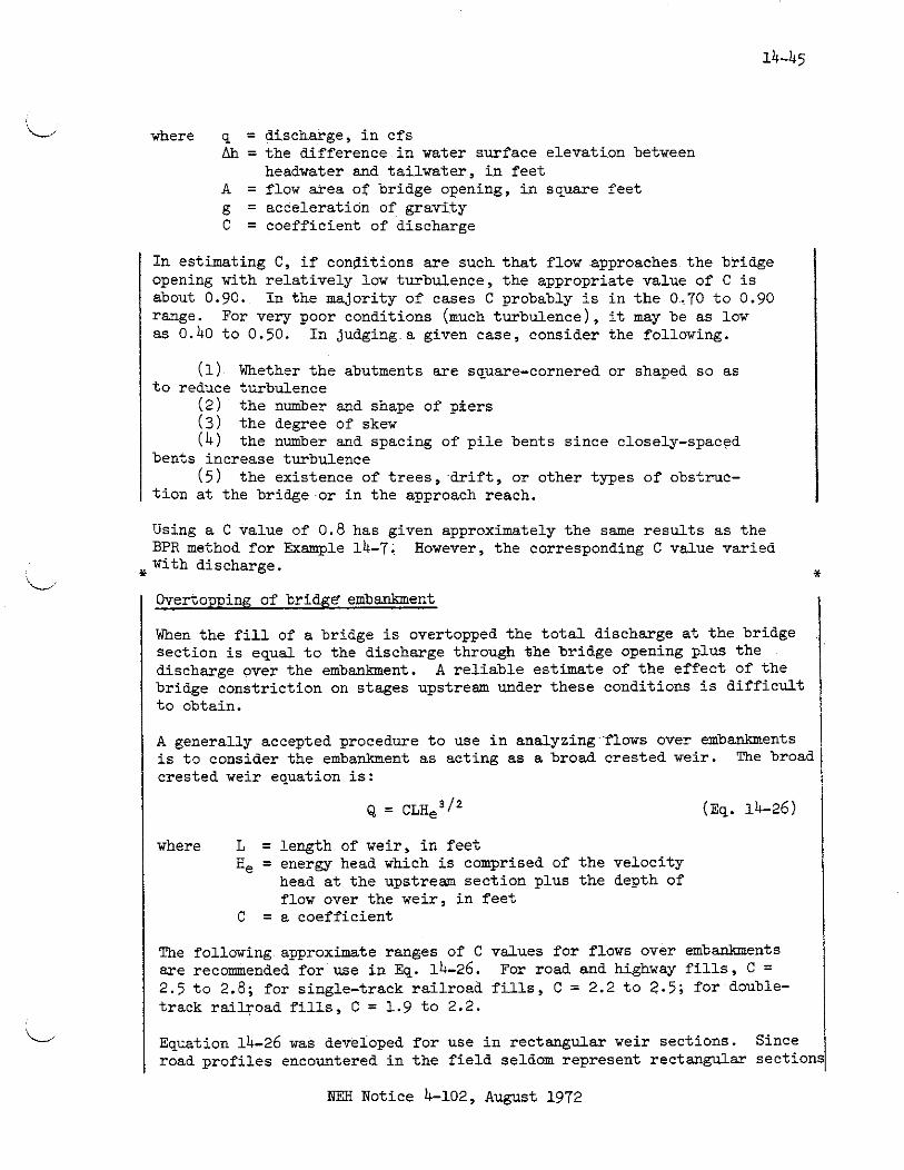
Overtopping of bridge embankment
When the f i l l of a bridge i s overtopped the t o t a l discharge a t the bridge section i s equal t o the discharge through %he bridge opening plus the discharge over the embankment. A re l iab le estimate of the effect of the bridge constriction on stages upstream under these conditions i s d i f f i cu l t t o obtain.
A generally accepted procedure t o use i n analyzing'flows over embankments i s t o consider the embankment as acting as a broad crested weir. The broad crested weir equation is:
where L = length of weir, i n fee t He = energy head which i s comprised of the velocity
head a t the upstream section plus the depth of flow over the weir, i n f ee t
C = a coefficient
The following approximate ranees of C values for flows over embanlrments are recommended for use i n Eq. 14-26. For road and highway f i l l s , C = 2.5 t o 2.8; for single-track ra i l road f i l l s , C = 2.2 t o 2.5; f o r double- track ra i l road f i l l s , C = 1.9 t o 2.2.
Equation 14-26 was developed for use i n rectangular weir sections. Since road prof i les encountered i n t he f i e l d seldom represent rectangular sectior
NM Notice 4-102, August 1972

it becomes difficult to determine the weir length to use. Many approaches have been formulated to approximate this length. One approach suggests measuring the top width at the maximum depth of flow over the road and - - computing A for each depth.
He = dc + - 2T
Another method suggests measuring the weir length from the cross section at an elevation equal to 5/6 of h above the low point on the embankment.
Amethod suggested for use in this chapter substitutes the flow area A for the weir length and flow depth over the weir in Eq. 14-26.
Then: Q = Cvbl/2 (Eq. 14-27)
where: A = flow area over the embankment at a given depth, h, in square feet
h = flow depth measured from the low point on the embankment, in feet
C ' = coefficient which accounts for the velocity of approach.
I The coefficient C' can be computed by equating Equations 14-26 and 14-27 and solving for C'.
1 depth
(Eq. 14-28)
= C[depth+velocity head
In Eq. 14-28 the depth is measured from the low point on the embankment of the bridge section and the velocity head is computed at the upstream section for the same elevation water is flowing over the embankment. The approach velocity may be approximatp3 by V = Q/A where Q is the total discharge and A is the total flow area at theupstream section for the given elwation. In cases where the approach velocity is sufficiently small C' will equal C and no correction for velocity head will be needed to use Equation 14-27.
The free discharge over the road computed using Eq. 14-27 must be modified when the tailwater elevation downstream is great enough to submerge the embankment of the bridge section. The modification to the free discharge, Qf, is made by computing a submergence ratio, &/HI, where X2 and R1 are the depths of water downstream and upstream, respectively, above the low point on the emb-ent. A submergence factor, R, is read from Figure 3-4 NEH-11, Drop Spillways, and the submerged discharge is computed as Qs = RQf. Then the total discharge at the bridge section is equal to the dis-
/ charge through the bridge opening plus the submerged discharge over the ; embankment. I I
1 Example 14-9 shows the use of Eq. 14-27 and Eq. 14-28 in computing flows j over embankments using a trial and error procedure to determine C'.
NEH Notice 4-102, August 1972

Example 14-9. Develoo a s t m e discharge curve for t he overflow section of the hiahway
A - - - - analyzed i n Example 14-8 (see Figure 14-12c) for the bridge opening of 300 fee t . The top of embankment i s a t elevation 107. Assume a C value of 2.7.
1. Select a range of elevations that w i l l define the ra t inn curve over the road. Tabulate i n column 1 of Table 14-7. The low point on the road i s a t elevation 107.
2. Compute the depth of flow, h , over the road. For each elevation l i s t e d i n column 1 compute h and l i s t i n column 2 of Table 14-7.
3. Compute hl/'. Tabulate i n column 3 of Table 14-7.
4. Compute the flow area, A, over the road. For each elevation l i s t ec i n column 1 compute the area over the road and tabulate i n column 4 of Table 14-7.
Steps 5 through 11 are used t o calculate the modified coeff ic ient , C ' t o account for t he approach velocity head. I f it i s determined tha t no modification t o the coefficient C i s required these steps may be omitted.
5. Compute the flow area a t the upstream section. For each elevation l i s t e d i n column 1 compute the t o t a l area a t the upstream section and tabulate i n column 5 of Table 14-7. The flow area can be obtained fromthe Kd computations a t the upstream section or computed d i rec t ly from the surveyed cross section.
6. Determine the discharge through the b r i d ~ e . For t he elevation i n column 1 read the discharge through the bridge opening previously Computed using bridge loss equations-and tabulate in column 6 of Table 14-7.
7 - Estimate the discharge over the road. Tabulate i n column 7 of Table 14-7.
8. List the t o t a l estimated discharge going past the bridge section. Sum columns 6 and 7 and tabulate i n column 8 of Table 14-7.
9. Compute the average velocity a t the upstream section. The velocity can be estimated by using the t o t a l upstream area from column 5 and the estimated discharge from column 8 for the eleva- t ions l i s t e d i n column 1 i n the equation V = Q/A. For example for elevation 107.5:
Tabulate the velocity i n column 9 of Table 14-7.
NEH Notice 4-102, August 1972

P C I
Table 14-7. Stage discharge over roadway at cross section M-4 without submergence. Example 14-9. .c- CJ
cfs I cfs
Q through bridge
Q est.ove: road
Q est. total cfs
(8)
26000
28300
32300 32200
37800
42000 45900
67800 69000
V
ft/se~
( 9 )
1.02
1.06
1.15 1.15
1.30
1.38 1.51
2.06 2.10
v2 - 2g
(10)
.016
.0175
.021
.021
.027
.03o
.035
.066
.068
C'
(11)
o 2.85
2.79 2.79
2.76
2.76 2.76
2.79 2.79
Q over road cfs
(12)
o 1300
4200 4200
8500
15600 156~0
36200 36200
Q total
cfs
(13)
26000
28300
32200
37900.
45900.
69000

Figure 14-17. Stage discharge with embankment overflow, sec t ion M-5, Example 14-9.

10. Codpute the velocity head. Using the velocity from column 9 compute V / 2 g and tabulate i n column 10 or Table 14-7.
11. Compute C' . Using equation 14-28 and data from Table 14-7 com- pute C ' , For example a t elevation 107.5:
L i s t C ' i n column 11 i n Table 14-7.
12. Compute discharge over the road. Using equation 14-27 and data from Table 14-7 compute t he discharge over the road. For example a t elevation 107.5:
Q = c ' A ~ ' / ' = 2.85(625)(.707) = 1260 c f s
Round t o 1300 cfs and l i s t i n column 12. Compare t h i s discharge valu t o the estimated discharge l i s t e a i n column 7. If the computed dis- charge i s l e s s than or greater than the estimated discharge modify the estimated discharge i n column 7 and recompute C ' following steps 8 through 12.
13. List the total 'discharge going past t he bridge section. Sum columns 6 and 12 a d Tabulate i n column 13 of Table 14-7.
14. Plot t he stage discharge curve. Using the computations shown i n columns 1 and 1 3 of Table 14-7 p lo t the elevation versus dis- charge. The portion of the di-scharge flowing over the road (col- umn 12) and the total. discharge curve i s shorn i n Figure 14-17 for t he 300 foot bridge. This i s the t o t a l stage discharge curve for the approach section (M-5).
Multiple bridge openings
Multiple openings i n roads occur quite often and must be considered different ly from single openings. The M r a t i o i n the BPR procedure is defined as:
Kd Bridge Kd Approach
When multiple openings are present the proper r a t i o must be assigned t o each opening and then the capacity computed accordingly. I f t he flow i s divided on the approach, the porblem i s then one of diVided flow with single openings in each channel. I n many cases the flow i s not divided
NEH Notice 4-102, August 1972

APPROACH FOR OPENING A APPROACH FOR OPENING B
When water elevation is at A approaches act as directed by the physical division point.
When water elevation is at B approaches act according to the ratio of KD's of openings.
Figure 14-18. Approach section for a bridge opening.

for overbank flows. In these cases the headwater elevation must be con- sidered t o be the same elevation for each opening and the solution becomes trial and error u n t i l the head losses are equal for each opening and the sum of the flows equals the desired to t a l .
The approaches are divided as shown i n Figure 14-18. When the headwater i s below the physical dividing point as i l l u s t r a t ed by Level A then the M r a t i o i s computed as i n a single opening.
When the headwater i s above the physical dividing point cross flow can Occur. When t h i s occurs t h e approach used t o compute t he M r a t i o and 3 i s as follows:
1. Compute the Kd value for each bridge opening.
2. Compute the Kd value for the t o t a l approach section.
3. Proportion the approach Kd value for each opening by the relationship:
Kd appr, = K%ridgex ....+ Ka,, . x t o t a l approach Kd.
'doridge 1 ' ' ' "%ridge2 rldge,
4. Compute M as before using the Kd value computed i n s tep 3 for the approach.
5. Compute the approach area contributing t o t h i s opening by the relationship:
Area apprx = '%ridgex x t o t a l approach
'%ridge 1 ....+% . ....
ridge* area
6. Compute J as before using the area computed i n s tep 5 for the approach area.
Culverts
Culverts of a l l types and s izes a?e encountered when computing stage discharge curves i n natural streams. These culverts may or may not have a s ignif icant effect on the development of a watershed work plan. However, i n many cases they present a problem i n evaluating a plan and must be analyzed t o determine i f an acceptable plan can be ins ta l led without enlarging or replacing the exist ing culvert.
The Bureau of Public Roads has developed procedures based on research data f o r use i n designing culverts. This document, Hydraulic Charts for the Selection of Highway Culverts, Hydraulic Engineering Circular No. 5, December 1965, i s available from the Superintendent of Documents, Washington, D. C.
IiEH Notice 4-102, August 1972
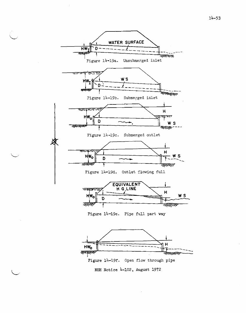
WATER SURFACE
~ i g u r e 14-1%. Unsubmerged i n l e t
-
Figure 14-19b. Submerged i n l e t
Figure 14-1%. Submerged ou t l e t
Figure 14-19d. Outlet flowing N 1
Figure 14-19e. Pipe f u l l par t way
Figure 14-19f. Open flow through pipe
NEH Notice 4-102, August 1972

Culverts of various types, ins ta l led under different conditions, were studied i n order t o develop procedures t o determine the backwater e f fec t for the two flow conditions: 1) culverts flowing with i n l e t control; 2 culverts flowing with ou t le t control.
In le t Control In l e t control means tha t the capacity of the culvert i s controlled a t the culvert entrance by the depth o f headwater (HWI) and the entrance geometry of the culvert including the barrel shape and cross sectional area and the type of i n l e t edge, shape of headwall, and other losses. With i n l e t control the entrance acts as an or i f ice and the bar re l of the culvert i s not subjected t o pressure flow. Figure 14.19a and 14.19b show sketches of two types of i n l e t controlled flow.
The nomographs shown on Exhibits 14-6 through 14-10 were developed from research data by the Division of Hydraulic Research, Bureau of Public Roads research data. They have been checked against actual measurements made by USGS with favorable resu l t s .
Types of In le t s . - The following descriptions are taken from "Electronic Computer Prograu for Hydraulic Analysis of Circular Culverts" Bureau of Public Roads, February 1969. Some of the types of i n l e t s are i l l u s t r a t ed - in Figure 14-20.
a. Tapered - This i n l e t i s a type of improved entrance with can be made of concrete or metal. Shapes are shown i n Figure 14-20a.
b. Bevel A and Bevel B - These bevels, a type of improved entrance, can be formed of concrete or metal.
c. Angled wingwall - Similar t o headwall but a t an angle with culvert .
d. Projecting - The culvert bar re l extends from the embanhent. The transverse section a t the i n l e t i s perpendicular t o the longitudinal axis of the culvert.
e. Headwall - A headwall i s a concrete or metal s t ructure placed around the entrance of the culvert . Headwalls considered are those giving a flush or square edge with the outside edge of the culvert bar re l . No dist inction i s made .for wingwals with skewed alignment.
f . Mitered - The end of the culvert barrel is on a miter or slope t o con- form with the fill slope. All degrees of miter are t rea ted a l i ke s ince research data on t h i s type of i n l e t are limited. Headwater i s measured from the culvert invert midway in to the mitered section.
g. End section - This section i s the common prefabricated end made of e i ther concrete or metal and placed on the i n l e t or ou t le t ends of a culvert. The closed portion of the section, i f present, i s not tapered. (Not i l l u s t r a t ed )
NEH Notice 4-102, Aug~s t 1972

NOTE1 WINGWALL lNGLEoF BOX CULVERT
INLET MAY OR FLARE \
MAY NOT BE BEVELED - Angled wing w a l l
, PLAN VIEW
0 SECTION A-A
T a ~ e r e d i n l e t
Bevel A and Bevel B
Figure
a SECTION 6.6
Projec t ing
Mitered
14-20. Types of cu lve r t i n l e t s .
NEH Notice 4-102, August 1972

h. Grooved edge - m e h e l l or socket end of a standard concrete pipe i s an example of t h i s entrance. (Not i l l u s t r a t ed )
Outlet Control Culverts flowing with ou t le t control can flow with the culvert bar re l f u l l or pa r t f u l l for par t of the ba r r e l length or for a l l of it. Figures 14-lgc, 14-lgd, 14-19e, and 14-19f show the various types of Outlet control flow. The equation and graphs for solving the equation give accurate r e su l t s for the first three conditions. For the fourth condition shown i n Figure 14-19f, the accuracy decreases as the head decreases. The head H, Figure 14-19c and 14-lgd, or the energy' required t o pass a given discharge through the culvert flowing i n out le t control with the bar re l flowing f u l l throughout i t s length consists of three major par ts : 1) velocity head Hv, 2 ) entrance loss He, and 3) f r i c t i on loss H f , a l l expressed i n fee t . From Figure 14-21a:
v2 Hv = when V i s the average velocity i n the culvert barrel .
g
He = entrance lo s s which depends on the geometry of the i n l e t . The loss i s expressed as a coefficient K, (Exhibit 14-21) times the ba r r e l velocity head.
Hf = f r i c t i on loss i n barrel
n = Mannings f r i c t i on factor L = length of culvert barrel ( f t ) V = velocity i n culvert bar re l ( f t / s ec ) g = acceleration of gravity ( f t / s ec2 ) R = hydraulic radius (ft)
Substi tuting i n Equation 14-23:
(Eq. 14-30)
(Eq. 14-32)
Figure 14-21a shows the terms of Eq. 14-29, the hydraulic gradeline, the energy gradeline, and the headwater depth HW,.
The expression for H i s derived by equating the t o t a l energy upstream from the culvert t o the energy just inside the culvert out le t .
NEH Notice 4-102, August 1972

Figure 14-21. Elements of culvert f l o w .
NER Notice 4-102, August 1972
From Figure 14-21a:
v If the velocity head i n the approach section i s low it
2g - can be ignored and HWo i s considered t o be the difference between the water surface and the invert of the culvert i n l e t .
The depth, d2, for culverts flowing f u l l i s equal t o the culvert height Figwe 14-19d, o r the ta i lwater depth (TW) whichever i s greater , Figure 14-21b.
The hydraulic gradeline f o r culverts flowing with the ba r r e l pa r t fu l l for pa r t of the bar re l length passes through a point where the water breaks with the top of the culvert and i f extended as a s t ra igh t l i n e w i l l pass through the plane o f t h e ou t le t end of the culvert a t a point above the c r i t i c a l depth. This point i s approximately hqlfway between dc and the crown of the culvert , or equal t o dc + D .
The depth d2 or ho 2
(See Figure 14-21c) for t h i s type of flow i s equal t o dc + D o r TW whichever i s greater.
- 2
With the above def ini t ion of d2 which w i l l be designated as ho, an equa- t ion common t o a l l out le t control conditions can be writ ten:
This equation w a s used t o develop the nomographs shown on Exhibits 14-11 through 14-15 which can be used t o develop stage discharge curves f o r the approach section t o culverts flowing with ou t le t control.
Exhibit 14-16 shows dc for discharge per foot of width for rectangular sections. Exhibits 14-17 t o 14-20 show dc for discharges for various non-rectangular culvert sections.
Example 14-10 Develop a stage discharge curve for cross section T-4 ( ~ i g u r e 14-4) show- ins, the backwater effect of e iaht 16' x 8' concrete box culver ts f o r each of-three conditions: 1) i n l e t Eontrol, 2) ou t le t control , present channel, and 3) out le t control , improved channel. Figure 14-22a shows a cross section along the centerline of the roadway at cross section T-3. Figure 14-22b shows a section through the roaaway with water surface prof i les pr ior t o and a f t e r the construction of the cvlverts and roadway embank- ment.
The culvert headwalls are para l le l t o the embankment with no wingrralls, and the entrance i s squafe on three edges.
The following are given i n t h i s example: a stage discharge curve f o r cross section T-2, present condition and with proposed channel improvement
NEH Notice 4-102, August 1972
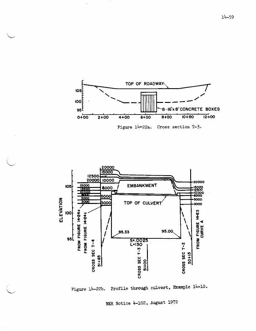
TOP OF ROADW
---- -16'~ 8'CONCRETE BOXES
OtOO 2 + 0 0 4 + 0 0 6+00 S t 0 0 l o t 6 0 12+00
Figure 14-22a. Cross section T-3.
TOP OF ROADWAY\ mr
---- 95 -16'~ 8'CONCRETE BOXES
OtOO 2 + 0 0 4 + 0 0 6+00 S t 0 0 l o t 6 0 12+00
TOP OF CULVER
v
Figure 14-22b. Profile through culvert, &le 14-10.
NM Notice 4-102, August 1972
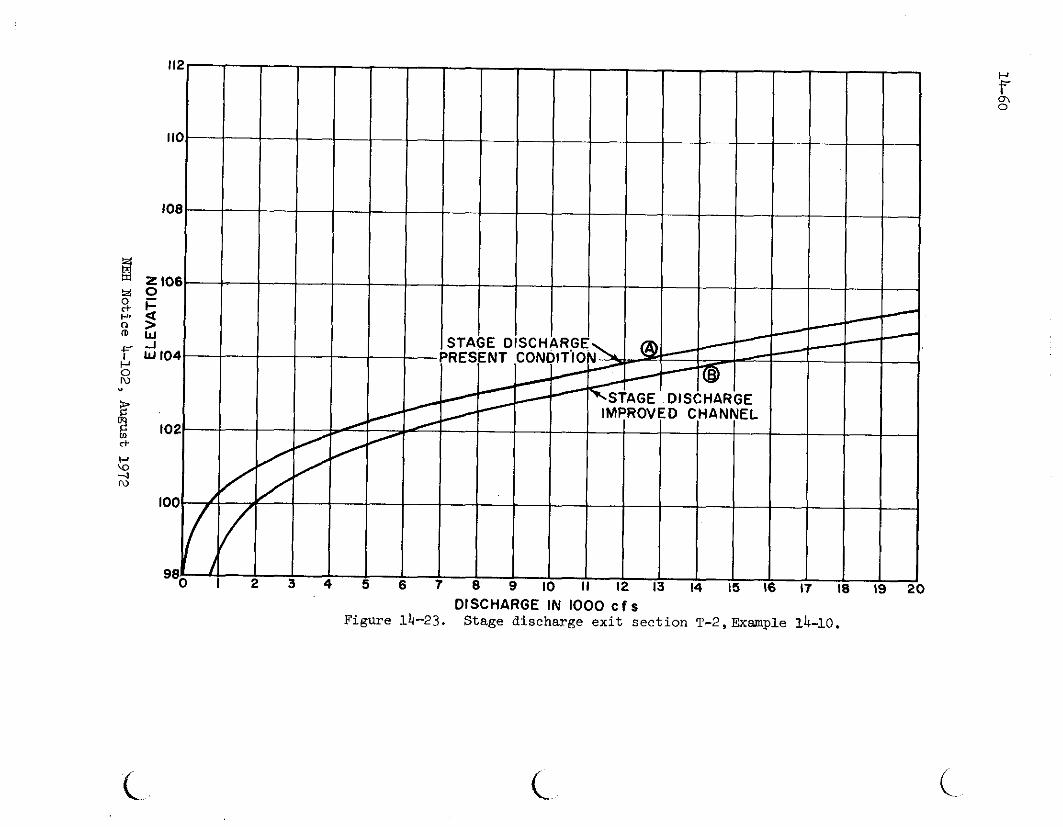
I DISC1 VT CON
f 9 1
GE DIS OVED C
$ 13 1
DISCHARGE IN 1000 c f s Figure 14-23. Stage discharge exit section T-2, Example 14-10.
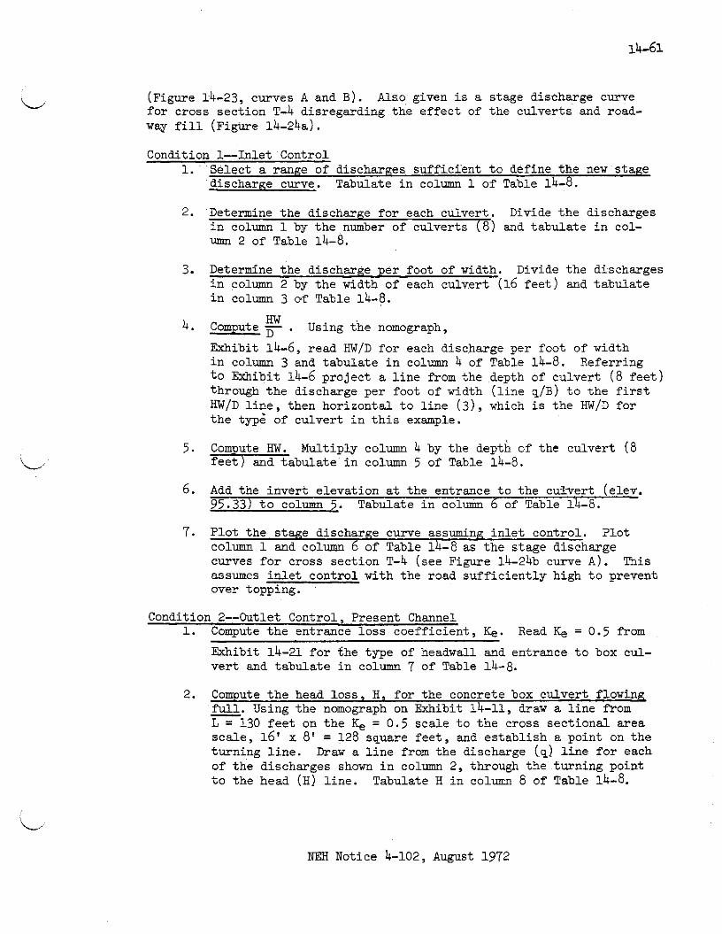
(Figure 14-23, curves A and B ) . Also given i s a stage discharge curve for cross section T-4 disregarding the effect of the culverts and road- way f i l l (Figure 14-24a).
Condition 1--Inlet Control Select a range of discharges sufficient t o define the new stage discharge curve. Tabulate i n column 1 of Table 14-8.
Determine the discharge f o r each culvert . Divide the discharges i n column 1 by the number of culverts (8) and tabulate i n col- umn 2 of able 14-8.
Determine the discharge per foot of width. Divide the discharges i n column 2 by the width of each culvert (16 f e e t ) and tabulate i n column 3 ok Table 14-8.
m Compute . Using the nomograph,
Exhibit 14-6, read HW/D for each discharge per foot of width i n column 3 and tabulate i n column 4 of Table 14-8. Referring t o Exhibit 14-6 project a l i n e from the depth of culvert ( 8 f ee t ) through the discharge per foot of width ( l i ne ~ I B ) t o the f i r s t HW/D l i n e , then horizontal t o l i n e ( 3 ) , which i s the HW/D for the typ6 of culvert i n t h i s example.
Com ute HW. Multiply column 4 by the depth of the culvert (8 e a b u l a t e i n column 5 of Table 14-8.
Add the inverc elevatior: ac the eneraxe t c che cu.lverc (elev. 95.33) t o column 5. Tabulate in column 6 of Table lh-6.
Plot the stage discharge curve assuming i n l e t control. Plot column 1 and column 6 of Table 14-8 as the stage discharge curves f o r cross section T-4 (see Figure 14-24b curve A ) . This assumes i n l e t control with the road suf f ic ien t ly high t o prevent over topping.
Condition 2--Outlet Control, Present Channel 1. Compute the entrance loss coeff ic ient , Ke. Read Ke = 0.5 from
Exhibit 14-21 f o r the type of headwall and entrance t o box cul- ver t and tabulate i n column 7 of Table 14-8.
2. Compute t he head loss , H, for the concrete box culvert flowing f u l l . Using the nomograph on Exhibit 14-11, draw a l i ne from - L = 130 f ee t on the L = 0.5 scale t o the cross sectional area scale: 16' x 8' = 128-square f ee t , and es tabl ish a point on the turning l i ne . Draw a l i n e from the discharge (q) l i n e for each of the discharges shown i n column 2, through the turning point t o the head (H) l ine . Tabulate H i n column 8 of Table 14-8.
NEH Notice 4-102, August 1972

Table 14-8. Headwater computations fo r eight 16' x 8' concrete box culver ts , headwalls pa ra l l e l t o embankment (no wingwalls) , square edged on three s ides , Example 14-10.
Each Culv. of Width z
" HY1 MI + 95.33 (invert elevation a t entrance end or culvert - 95.33). a g, ho - + 95.00 (invert elevation st outlet end of culvert m 95.00).
1/ MI, - H + lV - !& or H + ho - LS,, whichever i s greater.
% 4/ Tailwater elevation i s higher.th&m the computed elevation and open channel flow exis ts .
1-' 5/ 8ee cxanple on M i b i t 14-11. w -4 Note: with channel imPrwUent the control svitches from out le t t o i n l e t between 5000 N
and BOW ch.
see example on Exhibit 14-6.
81 If d, D, the outlet always controls. - do + D c m o t exceed D. -
2
- l I E:: Elev.
Outlet Control, Im~rove.3 Channel lV %
Elev. Elev.
(15) (16)
100.7 * y 101.6 101.87
102.6 103.8&
103.0 105.11
103.6 107.17
104.0 109.27
104.8 114.47

Compute the c r i t i c a l depth. dc. fo r each discharge per foot of width. - Using Exhibit 14-16, read dc for each discharge per foot Of width shown i n column 3 and tabulate i n column 9 of Tahle 14-8.
Compute + . Tabulate i n column 10 of Table 14-8 2
Note: dc + D cannot exceed D.
2
Compute ho. Add the inver t elevation of the ou t le t end of t he culvert (elev. 95.00) t o dc + D and tabulate as ho i n column 11 - of Table 14-8. 2
Compute the TW elevation for each discharge i n column 1. Using Figure 14-23, curve A, read the elevation for each discharge i n column 1 and tabulate as TW elevation i n column 12 of Table 14-8.
Compute the difference i n elevation of the i n l e t and out le t in- ver ts of the culverts. Multiply L x So = 130 x .0025 = 0.33 a d tabulate i n column 13 of Table 14-8.
Compute the water surface elevation, HWo, assuming out le t control.
Add values i n column 8 t o the la rger of column 11 or column 12 minus column 13 and tabulate as HWo i n column 1 4 of Table 14-8.
Plot the stage discharge curve assuming out le t control. Plot column 1 and column 1 4 on Figure 14-24c curve A assuming out le t control with the roadway suff ic ient ly high t o prevent over top- ping.
Condition 3-- Outlet Control, Improved Channel. 1. Compute the ta i lwater elevation a t the culvert for the improved
channel condition. Using F i m e 14-23. curve B. read the elevation for each discharge - - -, - i n column 1 and tabulate as-TW elevation i n column 1 5 of Table 14-8.
2. Compute the elevation assuming out le t control , improved channel. Add column 8 plus t he layer of column 1 5 or column 1 5 minus column 13 and-tabulate i n column 16 of Table 14-8.
3. Plot the stage discharge curve assuming out le t control with improved channel. Plot column 1 and column 16 on Figure 14-24d, curve A, as the stage discharge curve for cross section T-4 assuming out le t control with improved channel and the roadway suff ic ient ly high t o prevent over topping.
I Condition for flow over roadway. Assume the aporoach velocity head for t h i s example i s negligable and the . . coefficient. ' C a w i l l equal c'-used i n Eg. 14-26. -1f t he velocity head i s significant and a correction t o the coefficient C f s desired by using Eq. 14-27 follow steps 5 through 9 of Example 14-9.
NEH Notice 4-102, August 1972

Select a range of elevations t h a t w i l l define the ra t ing curve over the road. Tabulate i n column 1 of Table 14-9. The low point on the road i s a t elevation 106.
Compute the depth of f lou, H, over the road. For each elevation i n column 1 compute K and l i s t i n column 2 of Table 14-9.
Compute HI/'. Tabulate i n colunin 3 of Table 14-9.
Compute the flow area, A, over the road. or each elevation l i s t e d i n column 1 compute the area over the road and tabulate i n column 4 of Table 14-9.
Determine coefficient, C. Assume C = 2.7 for t h i s example and assume C = C1. Tabulate C' i n column 5 of Table 14-9.
Compute the discharge over the roadway using Eq. 14-26.
Plot the stage discharge curve. Using the computations shown i n Table 14-9 plot column 1 and column 6 shown on Figure 14-24b c , and d as curve B.
Graphically combine curves A and B -on Figures 14-24b, c and d t form the stage discharge curve f o r t he culver ts and weir flow w e r the roadway.
Table 14-9. Stage discharge over roadway a t cross section T-3, Figure 14-4. Example 14-10.
Elevation H / 2 A C ' 9
(1) ( 2 ) ( 3 ) ( 4 ) ( 5 ) (6)
Each of the 3 flow conditions were computed independent of each other. The flow condition t h a t actually controls i s tha t which requires t he greater upstream elevation for the discharge being considered. By com- paring elevations for the same discharge fir the 3 conditions tabulated on Table 14-8 and plot ted on Figure 14-24 b, c and d the type of control a t any given discharge can be determined. It may be advantageous t o plot a l l the curves on one graph t o be t te r define points of intersection.
NEII Notice 4-102, August 1972

DISCHARGE IN 1000 Cf 8
(a ) assuming no roadway i n place.
DISCHARGE IN 1000 CfS
( c ) o u t l e t con t ro l .
DISCHARGE IN 1000 c f 3
(b) i n l e t con t ro l
DISCHARGE IN 1000 Cfa
( d ) improved channel-outlet con t ro l
Figure 14-24. Rating curves c ross sec t ion T-4, Example 14-10.
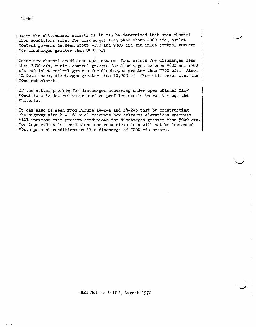
Under the old channel conditions it can be determined tha t open channel flow conditions ex i s t for discharges l e s s than about 4000 c f s , ou t le t control governs between about 4000 and 9Q00 cfs and i n l e t control governs for discharges greater than 9000 c fs .
Under new channel conditions open channel flow ex is t s for d i sch rges l e s s than 3800 c fs , ou t le t control governs for discharges between 3800 and 7300 cfs and i n l e t control govehs f o r discharges greater than 7300 cfs. Also, i n both cases, discharges greater than 10,200 cfs flow w i l l occur over the road embankment.
If the actual p rof i le for discharges occurring under open channel flow conditions i s desired water surface prof i les should be run through the Culverts.
It can also be seen from Figure 14-24a and 14-24b tha t by constructing the highway with 8 - 1 6 ' x 8' concrete box culverts elevations upstream w i l l increase over present conditions for discharges greater than 5000 c f s , fo r improved out le t conditions upstream elevations w i l l not be increased above present conditions u n t i l a discharge of 7200 cfs occurs.
NEH Notice 4-102, August 1972

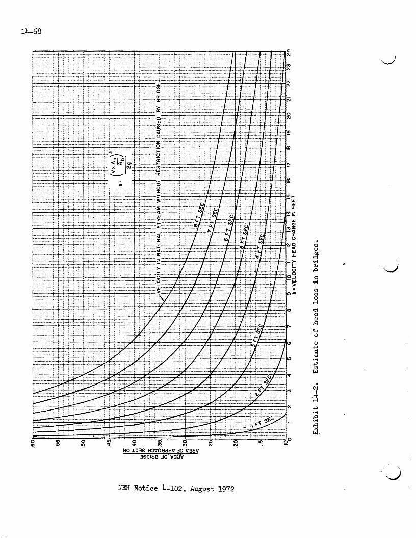
NEII Notice 4-102, August 1972
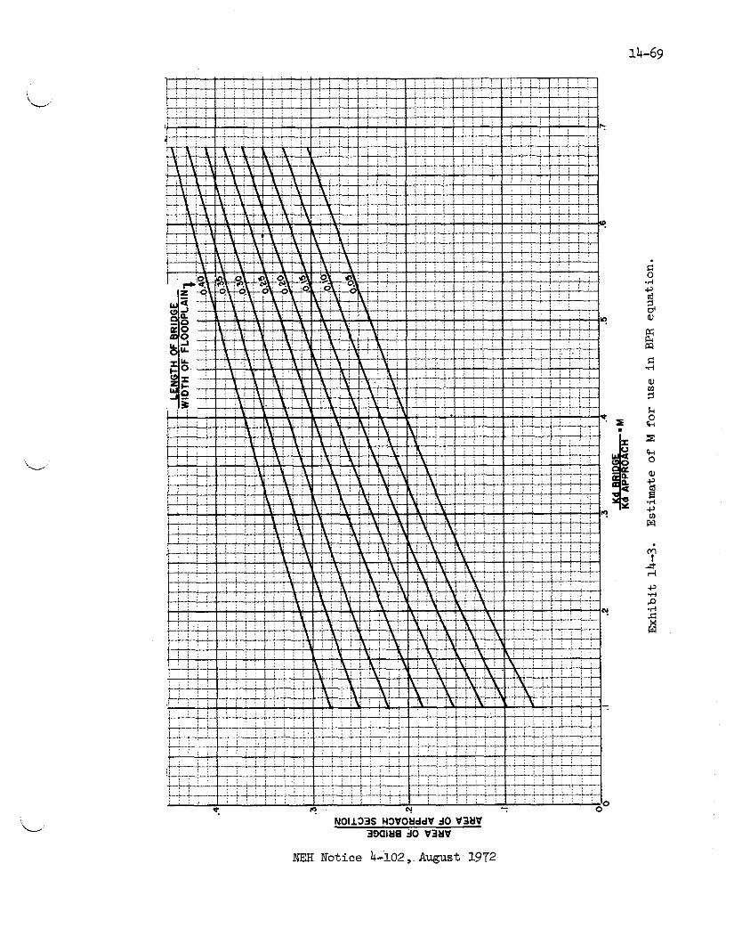
NEH Notice 4-102, August 1972

Exhibit 14-4. BPR base curve f o r bridges ( K ~ ) .

Exhibit 14-5. Incremental backwater coefficient for the more common types of columns, piers and p i l e bents.
NEH Notice 4-102, August 1972

Exhibit 14-6. Headwater c2epth for box culverts with i n l e t control.
NM Notice 4-102, August 1972
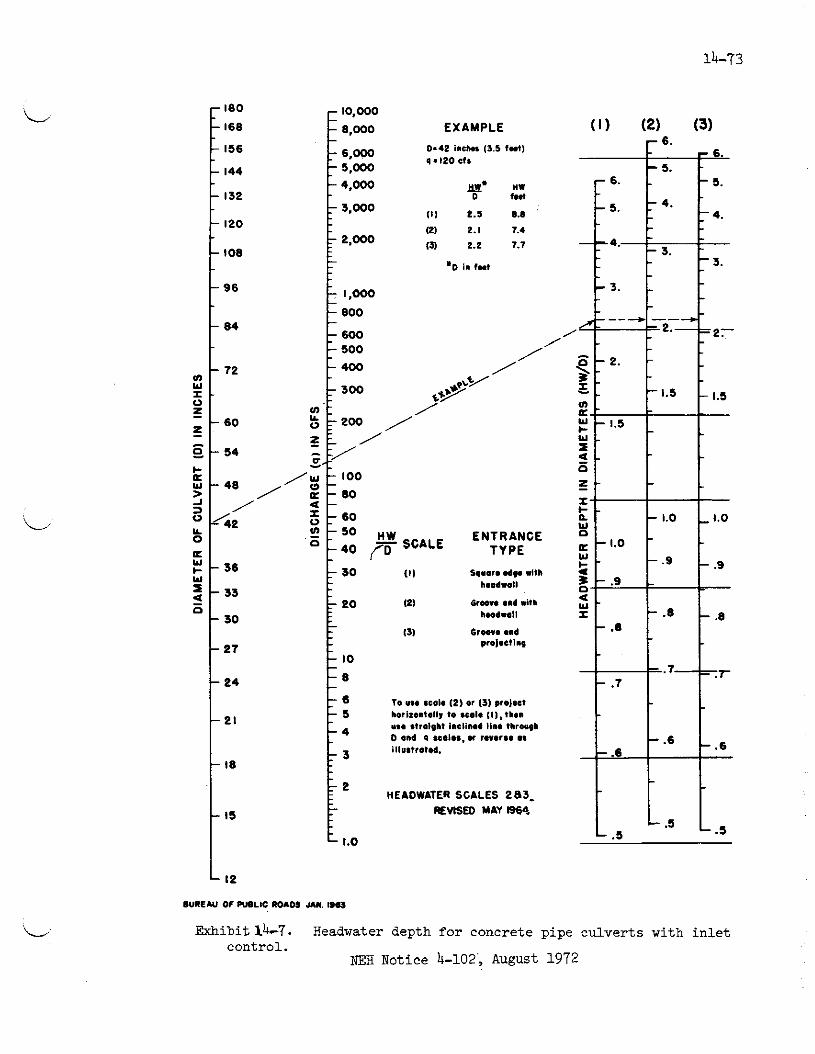
10.000 EXAMPLE
- 1,- - - 800 - - 600 - 500 - -00
/ / -
: 300 - m : / %:2@J / p E / - :/ Or
,/i \ I00
a - 80 4 - 3 :SO m - s o 0 1 4o SCALE
ENTRANCE TYPE
7
L I2
W R E N O f PWLIC ROADS JAN.
HEADWATER SCALES 283- REVISED MAY I964
Exhibit 14-7. Headwater depth f o r concrete pipe culver ts w i t h i n l e t control.
NEH Notice 4-102', August 1972

EXAMPLE' si.: 76.. 4k 0 .NO el,
E ( I ) P.8 11.2 (2) 2.2 0.8
1000 13) 1.3 9.Z
n & 1 coo z -80 - - 0 - 4 0 w ' 0 - 5 0 e - U - 40 2 -
0 :
- lo - - 0 - - 6 - 5 - 4
7 3 .
HV& ENTRANCE SCALE TYPE
Exhibit 14-8. Headwater depth for oval concrete pipe culver ts long axis horizontal with i n l e t control.
NM Notice 4-102, August 1972

EXAMPLE
0.36 Inoh. 13.0 fnt) q.66 C l l
HW SCALE ENTRANCE D TYPE
Exhibit 14-9. Headwater depth for C. M. pipe culverts with i n l e t control.
NEH Notice 4-102, August 1972

3.000 EXAMPLE
six.: 36.. 22' 2.000 q. 20rl.
Exhibit 14-10. Headwater depth f o r C.M. pipe-arch cu lve r t s with i n l e t control .
NEH Iiotice 4-102, A w s t 1972

Exhibit 14-11. Head for concrete box culverts flowing full n = 0.012.
NEH Notice 4-102, August 1972

" slow so- : Y l l l E l G E D OUTLET CUVEWT FU1IING FULL "* . ". lo-LSo
-
I - . w - 2 w Y
- Z - - x - 3 - - 0 . 4 - W - 4 I
- 5
- 6
- - 8 - -10
-
L 20
Exhibit 14-12. Head for concrete pipe culverts flowing Ail1 n = 0.012.
NEH Notice 4-102, August 1972

Exhibit 14-13. Head for oval concrete pipe culverts long axis horizontal or vertical flowing full n = 0.012.
NM Notice 4-102, August 1972
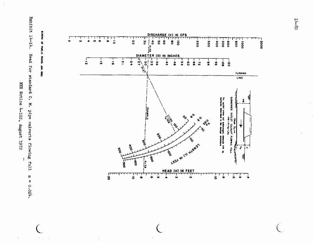
DISCHARGE ('4) IN CFS I ' I ' I ' I ' I I I I I ' " ' I " * ' N W L U O ) O - N
0 N
0 W + U O ) W - N
0 0 0 0 0 0 0 0 0 0 0 0 g ; 0
0 IE
HEAD (HI IN FEET
N 0
o m U L W N

UREAU OF M I C 80105 JAN. I963
W8YERtED OUILET CUVERT F M I N G FULL MW. whg-LS.
Exhibit 1b-15. Head f o r standard C. M. pipe-arch culverts flowing full n=0.024.
NEH Notice 4-102, August 1972

Exhibit 14-16. Critical depths-rectangular section.
NEH Notice 4-3-02, August 1972

DISCHARGE- 9 -CFS
BUREAU ff PUBLIC ROADS
J4N. 1964
Exhibit 14-17. Cr i t ica l depth. Circular pipe
NM Notice 4-102, August 1972

34
3.0
2.0
1.0
W W I&. I " 0 I
E 0 P 0 W
eo 40 60 eo 100 120 wo 180 zoo o DISCHARGE- q -CFS
2 o 7
k 0
6
5
4
3
2
I 0 1 0 0 200. 300 400 500 600 700 800 900 1000
DlSCHltRGE- q -CFS BUREAU W P ~ d ~ l t ROIDS
JAN. 1964
Exhibit 14-18. Critical depth. W a l concrete pipe. Long axis horizontal.
PJM Notice 4-102, Aug~st 1972
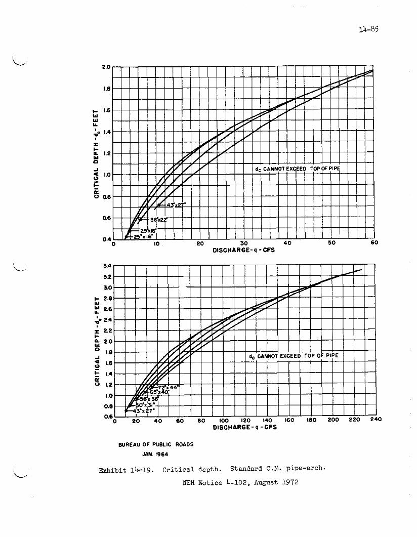
2.0
1.8
1.6 Y Y lb
2 1.4 x I- n 1.2 W a -I
1.0 0 'I 5 as
0.6
0.4 0 I0 20 30 40 50 60
DISCHARGE- q - CFS
3.4
s2
3 0
I- 2.8 Y 2 2.6
$ 2.4
1 2.2 I- : 2.0
1.8
a I 6 2 .
1.4 K 0 1.2
1.0
0.8
0.6 0 20 40 60 80 100 120 140 160 I80 200 220 240
DISCHARGE- q -CFS
BUREAU OF PUBLIC ROADS
JAN 1964
Exhibit 14-19. C r i t i c a l depth. Standard C.M. pipe-arch.
NEH Notice 4-102, August 1972

5
I- 4
w w Y
P I I-
ti s 0 J 4 0 C- a 0
2
I 0 I00 200 300 400 500 600
DISCHARGE- q -CFS
9
8
I- : 7 Y
.be 16 I- n W 0 J
5 4 0 C 4 a 0
3
2 0 200 400 600 800 1000 I200 1400 1600 1800 2000 2200 2400
DISCHARGE- q -CFS
BUREAU OF PUBLIC ROADS
JAN. 1964
Exhibit 1h-20. Cr i t i c a l depth. Structural p la te . C.M. pipe-arch.
iiEX Notice 4-102, August 1972

Exhibit 11;-21. Entrance loss coefrlcients.
v2 Coefficient ke t o apply t o velocity head - f o r determination of head
2g l o s s a t entrznce t o a structure, such as a culvert o r conduit, operat- ing f u l l o r p a r t l y full with control a t the out le t .
Entrance head lo s s & = k v2 z
.Pype of Structure and Iksign of Entrance - Pipe, Concrete
Coefficient ke
Projecting f roa f i l l , socket end (groove-end) . . . . . 0.2 Projecting from fill, sq. cut end . . . . . . . . . . . 0.5 Headwall o r headwall and w i n g w a l l s
Socket end of pipe (grooye-end) . . . . . . . . . . 0..2 Square-edge . . . . . . . . . . . . . . . . . . . . 0.5 Rounded (radius = 1 / 1 2 ~ ) . . . . . . . . . . . . . . 0.2
Mitered t o conform t o f i l l slope . . . . . . . . . . . . 0.7 ad-Sect ion conforming t o f i l l slope . . . . . . . . . . 0.5
Pipe, o r Pipe-Arch, Corrugated Metal
ProJecting from fill (no h e ~ d v a l l ) . . . . . . . . . . . 0.9 Headwall o r headwall and w i n g a l l s
Square-edge . . . . . . . . . . . . . . . . . . . . 0.5 Mitered t o conform t o f i l l slope . . . . . . . . . . . . 0.7 End-Section conforming t o f i l l slope . . . . . . . . . . 0.5
Box, Reinforced Concrete
Headwall parrillel to e m b a h e n t (no wingvdlls) Square-edged on 3 edges . . . . . . . . . . . . . . 0.5 Rounded on 3 edges t o radius of 1/12 bar re l a-ension . . . . . . . . . . . . . . . . . . . . . 0.2
W i i g h - a l l s a t 30' t o 75' t o bar re l Square-edged a t crown . . . . . . . . . . . . . . . 0.4 Crown edge roundetl t o radius of 1/12 bar re l dimension . . . . . . . . . . . . . . . . . . . . . 0.2
W i n p a l l s a t 10' t o 25' t o bar re l Square-edged a t crown . . . . . . . . . . . . . . . 0.5
Uirmgusl ls pa ra l l e l (extension of sides) Square-edged at crown . . . . . . . . . . . . . . . 0.7
NEH Notice 4-102, August 1972
