section 4: secondary ozone naaqs evaluation · standard (i.e., w126), we evaluated alternate...

S4-1

Section 4: Secondary Ozone NAAQS Evaluation

Synopsis

Exposure to ozone has been associated with a wide array of vegetation and ecosystem effects, including those that damage or impair the intended use of the plant or ecosystem. Such effects are considered adverse to the public welfare. Using a cumulative seasonal secondary standard (i.e., W126), we evaluated alternate standard levels at 7, 15, and 21 ppm-hours. EPA has not promulgated a distinct secondary NAAQS that is not identical to the primary NAAQS since the original SO2 regulation in 1970. Therefore, EPA has not previously conducted an analysis of the costs and benefits of attaining a secondary NAAQS, which is an exceptionally complex task. Complexities include determining which attainment year to analyze, whether to include emission reductions that occur as a result of implementing the primary NAAQS in the baseline for the secondary analysis, whether it is feasible to extrapolate beyond currently monitored counties, how to determine the amount of additional reductions needed to attain a secondary standard, whether nonattainment areas would include only areas that violate an air quality standard or also nearby areas that contribute to a violation, whether secondary standard nonattainment would require classification (as marginal, moderate, serious, etc), and whether the traditional nonattainment-area planning perspective would be successful for a secondary ozone standard. Because of these complexities as well as limited time and resources within the expedited schedule, we are limited in our ability to quantify the costs and benefits of attaining a separate secondary NAAQS for ozone for this proposal. However, we have incorporated a limited, qualitative assessment in this evaluation, including indicating which counties would have an additional burden to meet a secondary standard beyond the primary standard, and the qualitative benefits of reducing ozone exposure on forests, crops, and urban ornamentals. S4.1 Background

Exposure to ozone has been associated with a wide array of vegetation and ecosystem effects in the published literature (U.S. EPA, 2006). These effects include those that damage or impair the intended use of the plant or ecosystem. Such effects are considered adverse to the public welfare and can include reduced growth and/or biomass production in sensitive plant species, including forest trees, reduced crop yields, visible foliar injury, reduced plant vigor (e.g., increased susceptibility to harsh weather, disease, insect pest infestation, and competition), species composition shift, and changes in ecosystems and associated ecosystem services.

Vegetation effects research has shown that seasonal air quality indices that cumulate peak-weighted hourly ozone concentrations are the best candidates for relating exposure to plant

S4-2

growth effects (U.S. EPA, 2006). Based on this research, the Ozone Staff Paper (hereafter, “the Staff Paper”) concluded that the cumulative, seasonal index referred to as “W126” is the most appropriate index for relating vegetation response to ambient ozone exposures (U.S. EPA, 2007). Based on additional conclusions regarding appropriate diurnal and seasonal exposure windows, the Staff Paper recommended a cumulative seasonal secondary standard, expressed as an index of the annual sum of weighted hourly concentrations (using the W126 form), set at a level in the range of 7 to 21 ppm-hours. The index would be cumulated over the 12-hour daylight window (8:00 a.m. to 8:00 p.m.) during the consecutive 3-month period during the ozone season with the maximum index value (hereafter, referred to as the 12-hour, maximum 3-month W126). After reviewing the recommendations in the Staff Paper, EPA’s Clean Air Scientific Advisory committee (CASAC) agreed with the form of the secondary standard, but instead recommended a range of 7 to 15 ppm-hours (U.S. EPA-SAB, 2007).

S4.2 Air Quality Analysis

In this analysis, we considered the extent to which there is overlap between county-level air quality measured in terms of the 8-hour average form of the current secondary standard and that measured in terms of the 12-hour W126, alternative cumulative, seasonal form. These comparisons used 3-year averages, as well as using the 3-year average current 8-hour form and the annual W126 county-level air quality values using monitoring data collected from 2006 to 2008. These results are listed in Table S4-1, and the counties are mapped in Figures S4-1 through S4-3. When individual years are compared (e.g., using the annual W126 level) significant variability occurs between years in the degree of overlap between the numbers of counties meeting various levels of the 8-hour and W126 forms. Therefore, the degree of protection for vegetation provided by an 8-hour average form in terms of cumulative, seasonal exposures would not be expected to be consistent on a year-to-year basis.

S4-3

Table S4-1: Number of Counties Exceeding Various W126 Levels When Meeting Various Levels of

the 8-Hr Standard in 2006 to 2008*

Levels of 12-hr W126 (ppm-hrs)

8-Hour Level Met >21 >15 >7

0.075 ppm

3 (3 - 16)

27 (21 - 76)

250 (180 - 272)

0.070 ppm

1 (1 - 5)

9 (7 - 24)

84 (54 - 114)

0.065 ppm

1 (1 - 2)

4 (3 - 10)

29 (21 - 50)

0.060 ppm/0.055 ppm

1 (1 - 2)

4 (3 - 10)

25 (18 - 34)

* The top value in each box represents the number of counties meeting the 8-hour level based on 2006-2008 data but exceeding the W126 level based on a 3-year W126 average for the 2006-2008 period. The numbers in parentheses indicate the range in the number of counties that exceed the W126 level on an annual basis in one of the three years—2006, 2007, 2008– based on 1-year W126 values

. This range indicates significant interannual variability.

S4-4

Figure S4-1: Counties exceeding a W126 Level of 21ppm-hrs (based on 2006-2008 monitoring data)



Meets 0.055

ppm Meets 0.060

ppm Meets 0.065

ppm Meets 0.070

ppm Meets 0.075

ppm Exceeds

0.075 ppm Exceeds 21 ppm-hrs

(Figure 1) 1 county -- -- -- +2 counties (1 total) (1 total) (1 total) (1 total) (3 total)

Exceeds 15 ppm-hrs (Figure 2)

4 counties -- -- +5 counties +22 counties (4 total) (4 total) (4 total) (9 total) (27 total)

Exceeds 7 ppm-hrs (Figure 3)

25 counties -- +4 counties +55 counties +166 counties (25 total) (25 total) (29 total) (84 total) (250 total)

S4-5

In this analysis, we also projected the W126 levels in 2020 that would result from the modeled control strategy developed as part of the analysis of the primary standard, shown in Figure S4-4. The modeling methodology used to project W126 levels into the future utilizes the same approach as used to project design values of the primary standard, as described in EPA modeling guidance (U.S. EPA, 2007). Essentially, the relative response of the model between the 2020 modeled control strategy and a 2002 base case simulation was paired with ambient values of W126 consistent with the 2002 base. Additionally, EPA assessed the number of counties that are projected to attain the various primary standards in 2020 but would still exceed the various threshold W126 levels. These data are listed in Table S4- 2, and mapped in Figures S4-5 through S4-7. Because this projection approach is prefaced on ambient data, projections can only be made for counties with ozone monitoring data for the base period. As a result, Table S4-2 and the associated figures may not capture other, currently unmonitored, locations. Based on the current analysis, at all alternate standard levels evaluated in 2020, only one county would meet the primary standards but exceed 21 ppm-hours.

Table S4-2: Number of Counties Projected to Exceed Various W126 Levels While Meeting Various

Levels of the Primary Standard in the Control Strategy in 2020 a Levels of 12-hr W126 (ppm-hrs)

8-Hour Level Met > 21 > 15 > 7

0.075 ppm 1 11 125 0.070 ppm 1 7 93 0.065 ppm 0 3 43 0.060 ppm 0 1 10 0.055 ppm 0 0 2

a Does not include counties that do not meet the various standard alternatives in the modeled control strategy. As these projections are limited to with existing ozone monitoring data, there might be other non-monitored areas that would exceed the secondary standard while attaining the primary standard.

S4-6

Figure S4-4: Number of Counties Projected to Exceed [21/15/7] ppm-hrs in the Baseline and Modeled Control Strategy in 2020*

* These maps include additional counties beyond those shown in Table S4-2 or Figures S4-5 through S4-7 for two reasons. First, these maps include 45 counties that did not have complete monitoring data for the primary standard, which did not allow for a comparison with the secondary standard. Second, these maps include 21 counties that exceed a primary standard of 0.075 ppm after the modeled control strategy. Many of the counties projected to exceed a W126 level of 21 ppm-hrs are in the South Coast and San Joaquin areas of California, which are not required to attain the primary standards by 2020.

10 counties that exceed 21 ppm-hrs after the modeled control strategy in 2020

14 additional counties that exceed 15 ppm-hrs for a total of 24


551 counties that meet 7 ppm-hrs

10 counties that exceed 21 ppm-hrs in the baseline in 2020



509 counties that meet 7 ppm-hrs

S4-7

Figure S4-5: Counties exceeding a W126 Level of 21ppm-hrs while meeting various levels of the Primary Standard in the Control Strategy in 2020

Figure S4-6: Counties exceeding a W126 Level of 15ppm-hrs while meeting various levels of the

Primary Standard in the Control Strategy in 2020

Figure S4-7: Counties exceeding a W126 Level of 7ppm-hrs while meeting various levels of the

Primary Standard in the Control Strategy in 2020

Meets 0.055

ppm Meets 0.060

ppm Meets 0.065

ppm Meets 0.070

ppm Meets 0.075

ppm

Exceeds 21 ppm-hrs (Figure S4-5)

-- --

1 -- -- (1 total) (1 total)


1 county +2 counties +4 counties +4 counties -- (1 total) (3 total) (7 total) (11 total)


2 counties +8 counties +33 counties +50 counties +32 counties (2 total) (10 total) (43 total) (93 total) (125 total)

S4-8

As noted above, this analysis only projected W126 levels in 2020 where there are current ozone monitors. Due to the lack of more complete monitor coverage in many rural areas, this analysis might not be an accurate reflection of the situation in non-monitored, rural counties where important vegetation and ecosystems are located as well as areas of national public interest. This is an important consideration because: (1) the biological database stresses the importance of cumulative, seasonal exposures in determining plant response; (2) plants have not been specifically tested for the importance of daily maximum 8-hour ozone concentrations in relation to plant response; and (3) the effects of attainment of a 8-hour standard in upwind urban areas on rural air quality distributions cannot be characterized with confidence due to the lack of monitoring data in rural and remote areas (U.S. EPA, 2007). Many counties contain high elevation, rural or remote sites where ozone concentration distributions tend to be flatter. These areas may not reflect the typical urban and near-urban pattern of low morning and evening ozone concentrations with a high mid-day peak, but instead maintain relatively flat patterns with many concentrations in the mid-range (e.g., 0.05-0.09 ppm) for extended periods. Therefore, the potential for disconnect between 8-hour average and cumulative, seasonal forms is greater. Additional rural high elevation areas important for vegetation that are not currently monitored would likely experience similar ozone exposure patterns (U.S. EPA, 2007).

S4.3 Evaluation of Costs and Benefits of Attaining a Secondary Ozone NAAQS

The purpose of a secondary NAAQS is to protect the public welfare against the negative effects of criteria air pollutants from decreased visibility, damage to animals, crops, vegetation, and buildings. EPA has not promulgated a distinct secondary NAAQS that is not identical to the primary NAAQS since the original SO2 regulation in 1970. Therefore, EPA has not previously conducted an analysis of the costs and benefits of attaining a secondary NAAQS, which is an exceptionally complex task. First, it is unclear when an area would need to attain a secondary standard, which makes choosing an analysis year difficult. Whereas attainment dates for the primary NAAQS are explicitly designated in the CAA, the attainment dates for the secondary NAAQS are required “as expeditiously as practicable” after the nonattainment designation (42 USC §7502(a)(2)). As air quality improves over time, an area would not need as many emission reductions for a later analysis year as the area would need for a sooner analysis year. Therefore, the choice of an analysis year has a significant effect on the magnitude of the costs and benefits of attaining a secondary standard.

Second, it is unclear whether it is appropriate to include emission reductions that occur as

a result of implementing the primary NAAQS in the baseline for the secondary analysis. This is a critical decision, as it would either improperly ascribe the costs and benefits of the primary NAAQS to the secondary NAAQS or it would violate the requirements of OMB’s Circular A-4 to only include promulgated rules in the regulatory baseline.

S4-9

Third, the current monitoring network was not designed to adequately reflect W126 levels

in many areas of the county, especially the rural west. Therefore, it is difficult to extrapolate the concentrations beyond the currently monitored counties, and we would be unable to quantify the degree of nonattainment in many areas of the country that would be affected by the standard. Earlier this year, EPA proposed an expansion of the non-urban ozone monitoring network (74 FR 34525). If the regulation is finalized, three required non-urban monitors would be required in each State, beginning in 2012. Of those required monitors, at least one monitor was proposed to be located in areas of ecological value, such as National Parks, wilderness areas, or areas of sensitive national vegetation and ecosystems. We note, however, that even after the initial deployment of these additional monitors, it may prove challenging to completely characterize ozone concentrations in some locations that have not traditionally been areas of focus for ozone network deployment.

Fourth, as shown in Figure S4-4, a large number of counties are projected to not to meet

the various potential secondary standards in 2020 even after the substantial controls in the hypothetical RIA control scenario. Estimating the amount of additional reductions (extrapolated tons) needed to attain a secondary standard would require a better understanding of the relationship between emissions reductions and the W126 metric. Our long experience with the primary standard allows us to use simple impact ratios with some confidence in the extrapolated cost analysis for the primary standard. At present, it is not possible to reproduce a similar analysis for the secondary standard.

Fifth, EPA has not yet developed draft guidance for States to recommend boundaries of

nonattainment areas for a secondary ozone nonattainment area. The Clean Air Act (CAA) requires that nonattainment areas include not only areas that violate an air quality standard but also nearby areas that contribute to a violation. Many of the areas that would violate a secondary ozone standard without violating the primary ozone standard appear to be located in rural areas. Many of these areas lack significant sources of emissions of ozone precursors within the potential nonattainment area, so the cause of the violation is likely due to longer-range transport of ozone and precursors. Analyses of the origin of the contributing emissions in such areas is still incomplete, so it is unclear how large to make these nonattainment areas to afford the kind of protection to the sensitive species of vegetation that the standard is designed to protect while including the nearby sources that may be contributing to the violation and excluding contributing sources that are not “nearby.”

Sixth, EPA has not yet developed draft guidance to States on how they should develop their

secondary standard SIPs and anticipate for the implementation proposal setting forth an open-ended solicitation of comments on how that should be done, rather than propose specific

S4-10

guidance. One issue that must be addressed from a legal stand point is whether planning for nonattainment areas must be done under the more prescriptive subpart 2 requirements of the CAA, which would require classification (as marginal, moderate, serious, etc). The CAA language is unclear as to whether subpart 2 applies to nonattainment areas under a secondary standard (although it appears to be clear that the maximum statutory attainment dates in the classification table only apply to the “primary” standard). The agency has never faced this issue in the past for ozone, so there is no precedent and would have to be addressed in rulemaking.

Seventh, it does not appear that the traditional nonattainment-area planning perspective

would be very successful for addressing the violations based on the areas that currently violate the various options for a secondary ozone standard. Many of the potential nonattainment areas are in rural areas, many without significant sources of emissions of ozone precursors within the potential nonattainment area, and likely due to longer-range transport of ozone and precursors. An analysis of the origin of the contributing emissions in such areas is still incomplete, so it is unclear from a practical standpoint how SIPs would be developed. In some cases, multi-state plans might need to be developed to address the violations. This may even possibly entail EPA establishment under CAA section 176A of an interstate transport commission to address the problem.

Because of these complexities as well as limited time and resources within the expedited

schedule, we are limited in our ability to quantify the costs and benefits of attaining a separate secondary NAAQS for ozone for this proposal. However, we have incorporated a limited, qualitative assessment in this analysis, including indicating which counties would have an additional burden to meet a secondary standard beyond the primary standard, and the qualitative benefits of reducing ozone exposure on forests, crops, and urban ornamentals. S4.4 Benefits of Reducing Ozone Effects on Vegetation and Ecosystems1

Ozone causes discernible injury to a wide array of vegetation (U.S. EPA, 2006; Fox and

Mickler, 1996). In terms of forest productivity and ecosystem diversity, ozone may be the pollutant with the greatest potential for regional-scale forest impacts (U.S. EPA, 2006). Studies have demonstrated repeatedly that ozone concentrations commonly observed in polluted areas can have substantial impacts on plant function (De Steiguer et al., 1990; Pye, 1988).

When ozone is present in the air, it can enter the leaves of plants, where it can cause significant cellular damage. Like carbon dioxide (CO2) and other gaseous substances, ozone enters plant tissues primarily through the stomata in leaves in a process called “uptake” (Winner and

1 It is important to note that these vegetation benefits are contingent upon the secondary standard being the controlling standard. In other words, if the primary standard is controlling in all areas, there would not be any additional vegetation benefits beyond those due to the primary standard.

S4-11

Atkinson, 1986). Once sufficient levels of ozone (a highly reactive substance), or its reaction products, reaches the interior of plant cells, it can inhibit or damage essential cellular components and functions, including enzyme activities, lipids, and cellular membranes, disrupting the plant's osmotic (i.e., water) balance and energy utilization patterns (U.S. EPA, 2006; Tingey and Taylor, 1982). With fewer resources available, the plant reallocates existing resources away from root growth and storage, above ground growth or yield, and reproductive processes, toward leaf repair and maintenance, leading to reduced growth and/or reproduction. Studies have shown that plants stressed in these ways may exhibit a general loss of vigor, which can lead to secondary impacts that modify plants' responses to other environmental factors. Specifically, plants may become more sensitive to other air pollutants, or more susceptible to disease, pest infestation, harsh weather (e.g., drought, frost) and other environmental stresses, which can all produce a loss in plant vigor in ozone-sensitive species that over time may lead to premature plant death. Furthermore, there is evidence that ozone can interfere with the formation of mycorrhiza, essential symbiotic fungi associated with the roots of most terrestrial plants, by reducing the amount of carbon available for transfer from the host to the symbiont (U.S. EPA, 2006).

This ozone damage may or may not be accompanied by visible injury on leaves, and likewise, visible foliar injury may or may not be a symptom of the other types of plant damage described above. Foliar injury is usually the first visible sign of injury to plants from ozone exposure and indicates impaired physiological processes in the leaves (Grulke, 2003). When visible injury is present, it is commonly manifested as chlorotic or necrotic spots, and/or increased leaf senescence (accelerated leaf aging). Because ozone damage can consist of visible injury to leaves, it can also reduce the aesthetic value of ornamental vegetation and trees in urban landscapes, and negatively affects scenic vistas in protected natural areas. Ozone can produce both acute and chronic injury in sensitive species depending on the concentration level and the duration of the exposure. Ozone effects also tend to accumulate over the growing season of the plant, so that even lower concentrations experienced for a longer duration have the potential to create chronic stress on sensitive vegetation. Not all plants, however, are equally sensitive to ozone. Much of the variation in sensitivity between individual plants or whole species is related to the plant’s ability to regulate the extent of gas exchange via leaf stomata (e.g., avoidance of ozone uptake through closure of stomata) (U.S. EPA, 2006; Winner, 1994). After injuries have occurred, plants may be capable of repairing the damage to a limited extent (U.S. EPA, 2006). Because of the differing sensitivities among plants to ozone, ozone pollution can also exert a selective pressure that leads to changes in plant community composition. Given the range of plant sensitivities and the fact that numerous other environmental factors modify plant uptake and response to ozone, it is not possible to identify threshold values above which ozone is consistently toxic for all plants.

S4-12

Because plants are at the base of the food web in many ecosystems, changes to the plant community can affect associated organisms and ecosystems (including the suitability of habitats that support threatened or endangered species and below ground organisms living in the root zone). Ozone impacts at the community and ecosystem level vary widely depending upon numerous factors, including concentration and temporal variation of tropospheric ozone, species composition, soil properties and climatic factors (U.S. EPA, 2006). In most instances, responses to chronic or recurrent exposure in forested ecosystems are subtle and not observable for many years. These injuries can cause stand-level forest decline in sensitive ecosystems (U.S. EPA, 2006, McBride et al., 1985; Miller et al., 1982). It is not yet possible to predict ecosystem responses to ozone with much certainty; however, considerable knowledge of potential ecosystem responses has been acquired through long-term observations in highly damaged forests in the United States (U.S EPA, 2006). Ozone Effects on Forests

Air pollution can affect the environment and affect ecological systems, leading to changes in the ecological community and influencing the diversity, health, and vigor of individual species (U.S. EPA, 2006). Ozone has been shown in numerous studies to have a strong effect on the health of many plants, including a variety of commercial and ecologically important forest tree species throughout the United States (U.S. EPA, 2007).

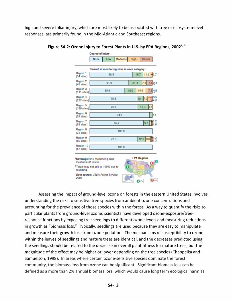
In the U.S., this data comes from the U.S. Department of Agriculture (USDA) Forest Service Forest Inventory and Analysis (FIA) program. As part of its Phase 3 program, formerly known as Forest Health Monitoring, FIA examines ozone injury to ozone-sensitive plant species at ground monitoring sites in forestland across the country (excluding woodlots and urban trees). FIA looks for damage on the foliage of ozone-sensitive forest plant species at each site that meets certain minimum criteria. Because ozone injury is cumulative over the course of the growing season, examinations are conducted in July and August, when ozone injury is typically highest. Monitoring of ozone injury to plants by the USDA Forest Service has expanded over the last 10 years from monitoring sites in 10 states in 1994 to nearly 1,000 monitoring sites in 41 states in 2002. The data underlying the indictor in Figure S4-2 are based on averages of all observations collected in 2002, the latest year for which data are publicly available at the time the study was conducted, and are broken down by U.S. EPA Regions. Ozone damage to forest plants is classified using a subjective five-category biosite index based on expert opinion, but designed to be equivalent from site to site. Ranges of biosite values translate to no injury, low or moderate foliar injury (visible foliar injury to highly sensitive or moderately sensitive plants, respectively), and high or severe foliar injury, which would be expected to result in tree-level or ecosystem-level responses, respectively (U.S. EPA, 2006; Coulston, 2004). The highest percentages of observed

S4-13

high and severe foliar injury, which are most likely to be associated with tree or ecosystem-level responses, are primarily found in the Mid-Atlantic and Southeast regions.

Figure S4-2: Ozone Injury to Forest Plants in U.S. by EPA Regions, 2002a, b

Assessing the impact of ground-level ozone on forests in the eastern United States involves understanding the risks to sensitive tree species from ambient ozone concentrations and accounting for the prevalence of those species within the forest. As a way to quantify the risks to particular plants from ground-level ozone, scientists have developed ozone-exposure/tree-response functions by exposing tree seedlings to different ozone levels and measuring reductions in growth as “biomass loss.” Typically, seedlings are used because they are easy to manipulate and measure their growth loss from ozone pollution. The mechanisms of susceptibility to ozone within the leaves of seedlings and mature trees are identical, and the decreases predicted using the seedlings should be related to the decrease in overall plant fitness for mature trees, but the magnitude of the effect may be higher or lower depending on the tree species (Chappelka and Samuelson, 1998). In areas where certain ozone-sensitive species dominate the forest community, the biomass loss from ozone can be significant. Significant biomass loss can be defined as a more than 2% annual biomass loss, which would cause long term ecological harm as

S4-14

the short-term negative effects on seedlings compound to affect long-term forest health (Heck, 1997).

Some of the common tree species in the United States that are sensitive to ozone are black cherry (Prunus serotina), tulip-poplar (Liriodendron tulipifera), and eastern white pine (Pinus strobus). Ozone-exposure/tree-response functions have been developed for each of these tree species, as well as for aspen (Populus tremuliodes), and ponderosa pine (Pinus ponderosa) (U.S. EPA, 2007). Other common tree species, such as oak (Quercus spp.) and hickory (Carya spp.), are not nearly as sensitive to ozone. Consequently, with knowledge of the distribution of sensitive species and the level of ozone at particular locations, it is possible to estimate a “biomass loss” for each species across their range. As shown in Figure S4-3, current ambient levels of ozone are associated with significant biomass loss across large geographic areas (U.S. EPA, 2009b). However, this information is unavailable for a future analysis year or incremental to a specified control strategy.

To estimate the biomass loss for forest ecosystems across the eastern United States, the

biomass loss for each of the seven tree species was calculated using the three-month, 12-hour W126 exposure metric at each location, along with each tree’s individual C-R functions. The W126 exposure metric was calculated using monitored ozone data from CASTNET and AQS sites, and a three-year average was used to mitigate the effect of variations in meteorological and soil moisture conditions. The biomass loss estimate for each species was then multiplied by its prevalence in the forest community using the U.S. Department of Agriculture (USDA) Forest Service IV index of tree abundance calculated from Forest Inventory and Analysis (FIA) measurements (Prasad, 2003). Sources of uncertainty include the ozone-exposure/plant-response functions, the tree abundance index, and other factors (e.g., soil moisture). Although these factors were not considered, they can affect ozone damage (Chappelka, 1998).

S4-15

Figure S4-3: Estimated Black Cherry, Yellow Poplar, Sugar Maple, Eastern White Pine, Virginia Pine, Red Maple, and Quaking Aspen Biomass Loss due to Current Ozone Exposure, 2006-2008

(U.S. EPA, 2009b)

Ozone damage to the plants including the trees and understory in a forest can affect the

ability of the forest to sustain suitable habitat for associated species particularly threatened and endangered species that have existence value – a nonuse ecosystem service - for the public. Similarly, damage to trees and the loss of biomass can affect the forest’s provisioning services in the form of timber for various commercial uses. In addition, ozone can cause discoloration of leaves and more rapid senescence (early shedding of leaves), which could negatively affect fall-color tourism because the fall foliage would be less available or less attractive. Beyond the aesthetic damage to fall color vistas, forests provide the public with many other recreational and educational services that may be impacted by reduced forest health including hiking, wildlife viewing (including bird watching), camping, picnicking, and hunting. Another potential effect of biomass loss in forests is the subsequent loss of climate regulation service in the form of reduced ability to sequester carbon.

Ozone Effects on Crops and Urban Ornamentals Laboratory and field experiments have also shown reductions in yields for agronomic crops exposed to ozone, including vegetables (e.g., lettuce) and field crops (e.g., cotton and wheat).

S4-16

Damage to crops from ozone exposures includes yield losses (i.e., in terms of weight, number, or size of the plant part that is harvested), as well as changes in crop quality (i.e., physical appearance, chemical composition, or the ability to withstand storage) (U.S. EPA, 2007). The most extensive field experiments, conducted under the National Crop Loss Assessment Network (NCLAN) examined 15 species and numerous cultivars. The NCLAN results show that “several economically important crop species are sensitive to ozone levels typical of those found in the United States” (U.S. EPA, 2006). In addition, economic studies have shown reduced economic benefits as a result of predicted reductions in crop yields, directly affecting the amount and quality of the provisioning service provided by the crops in question, associated with observed ozone levels (Kopp et al, 1985; Adams et al., 1986; Adams et al., 1989). According to the Ozone Staff Paper, there has been no evidence that crops are becoming more tolerant of ozone (U.S. EPA, 2007). Using the Agriculture Simulation Model (AGSIM) (Taylor, 1994) to calculate the agricultural benefits of reductions in ozone exposure, U.S. EPA estimated that meeting a W126 standard of 21 ppm-hr would produce monetized benefits of approximately $160 million to $300 million (inflated to 2006 dollars) (U.S. EPA, 2007). Urban ornamentals are an additional vegetation category likely to experience some degree of negative effects associated with exposure to ambient ozone levels. Because ozone causes visible foliar injury, the aesthetic value of ornamentals (such as petunia, geranium, and poinsettia) in urban landscapes would be reduced (U.S. EPA, 2007). Sensitive ornamental species would require more frequent replacement and/or increased maintenance (fertilizer or pesticide application) to maintain the desired appearance because of exposure to ambient ozone (U.S. EPA, 2007). In addition, many businesses rely on healthy-looking vegetation for their livelihoods (e.g., horticulturalists, landscapers, Christmas tree growers, farmers of leafy crops, etc.) and a variety of ornamental species have been listed as sensitive to ozone (Abt Associates, 1995). The ornamental landscaping industry is valued at more than $30 billion (inflated to 2006 dollars) annually, by both private property owners/tenants and by governmental units responsible for public areas (Abt Associates, 1995). Therefore, urban ornamentals represent a potentially large unquantified benefit category. This aesthetic damage may affect the enjoyment of urban parks by the public and homeowners’ enjoyment of their landscaping and gardening activities. In addition, homeowners may experience a reduction in home value or a home may linger on the market longer due to decreased aesthetic appeal. In the absence of adequate exposure-response functions and economic damage functions for the potential range of effects relevant to these types of vegetation, we cannot conduct a quantitative analysis to estimate these effects.

S4-17

Other ozone co-benefits In addition to the direct benefits on vegetation that the secondary ozone NAAQS is intended to produce, there are many other benefits from reducing ambient ozone concentrations.2 Controlling ozone concentrations is associated with significant human health benefits, including mortality and respiratory morbidity. 3 In addition, controlling ozone precursor pollutants (i.e., NOX) would reduce respiratory effects, reduce aquatic and terrestrial acidification, reduce excess aquatic and terrestrial nutrient enrichment, and improve visibility.4 Furthermore, NOX and VOCs are also precursors to PM2.5, which would lead to reductions in human health effects including mortality, respiratory morbidity, and cardiovascular morbidity.5

S4.5 References Abt Associates, Inc. 1995. Urban ornamental plants: sensitivity to ozone and potential economic

losses. U.S. EPA, Office of Air Quality Planning and Standards, Research Triangle Park. Under contract to RADIAN Corporation, contract no. 68-D3-0033, WA no. 6. pp. 9-10.

Adams, R. M., Glyer, J. D., Johnson, S. L., McCarl, B. A. 1989. A reassessment of the economic

effects of ozone on U.S. agriculture. Journal of the Air Pollution Control Association, 39, 960-968.

Adams, R. M., Hamilton, S. A., McCarl, B. A. 1986. The benefits of pollution control: the case of ozone and U.S. agriculture. American Journal of Agricultural Economics, 34, 3-19.

Chappelka, A.H., Samuelson, L.J. 1998. Ambient ozone effects on forest trees of the eastern

United States: a review. New Phytologist, 139, 91-108.

Coulston, J.W., Riitters, K.H., Smith, G.C. 2004. A preliminary assessment of the Montreal process indicators of air pollution for the United States. Environmental Monitoring and Assessment, 95, 57-74.

2 It is important to note that these health benefits are contingent upon the secondary standard being the controlling standard. In other words, if the primary standard is controlling in all areas, there would not be any additional health benefits beyond those due to the primary standard. 3 See the Chapter 6 of the 2008 RIA, the updated benefits analysis in Section 3 of this supplemental, and the Ozone Staff Paper (U.S. EPA, 2007) for additional information on the health effects of ozone. 4 See the Integrated Science Assessment for Oxides of Nitrogen: Health Criteria (U.S. EPA, 2008a) for more information on the health effects of NO2 and the Integrated Science Assessment for Oxides of Nitrogen and Sulfur - Ecological Criteria (U.S. EPA, 2008b) for more information on the ecological effects of NO2. 5 See Chapter 6 of the 2008 RIA, the updated benefits analysis in Section 3 of this supplemental, and the PM Integrated Science Assessment (U.S. EPA, 2009) for additional information on the health effects of fine particles.

S4-18

De Steiguer, J., Pye, J., Love, C. 1990. Air Pollution Damage to U.S. Forests. Journal of Forestry, 88(8), 17-22.

Fox, S., Mickler, R. A. (Eds.). 1996. Impact of Air Pollutants on Southern Pine Forests, Ecological

Studies. (Vol. 118, 513 pp.) New York: Springer-Verlag. Grulke, N.E. 2003. The physiological basis of ozone injury assessment attributes in Sierran

conifers. In A. Bytnerowicz, M.J. Arbaugh, & R. Alonso (Eds.), Ozone air pollution in the Sierra Nevada: Distribution and effects on forests. (pp. 55-81). New York, NY: Elsevier Science, Ltd.

Heck, W.W. &Cowling E.B. 1997. The need for a long term cumulative secondary ozone standard –

an ecological perspective. Environmental Management, January, 23-33.

Kopp, R. J., Vaughn, W. J., Hazilla, M., Carson, R. 1985. Implications of environmental policy for U.S. agriculture: the case of ambient ozone standards. Journal of Environmental Management, 20, 321-331.

McBride, J.R., Miller, P.R., Laven, R.D. 1985. Effects of oxidant air pollutants on forest succession

in the mixed conifer forest type of southern California. In: Air Pollutants Effects on Forest Ecosystems, Symposium Proceedings, St. P, 1985, p. 157-167.

Miller, P.R., O.C. Taylor, R.G. Wilhour. 1982. Oxidant air pollution effects on a western coniferous

forest ecosystem. Corvallis, OR: U.S. Environmental Protection Agency, Environmental Research Laboratory (EPA600-D-82-276).

Prasad, A.M. and Iverson, L.R. 2003. Little’s range and FIA importance value database for 135

eastern U.S. tree species. Northeastern Research Station, USDA Forest Service. Available on the Internet at http://www.fs.fed.us/ne/delaware/4153/global/littlefia/index.html

Pye, J.M. 1988. Impact of ozone on the growth and yield of trees: A review. Journal of

Environmental Quality, 17, 347-360. Smith, G., Coulston, J., Jepsen, E., Prichard, T. 2003. A national ozone biomonitoring program—

results from field surveys of ozone sensitive plants in Northeastern forests (1994-2000). Environmental Monitoring and Assessment, 87, 271-291.

Taylor R. 1994. Deterministic versus stochastic evaluation of the aggregate economic effects of

price support programs. Agricultural Systems 44: 461-473.

S4-19

Tingey, D.T., and Taylor, G.E. 1982 Variation in plant response to ozone: a conceptual model of physiological events. In M.H. Unsworth & D.P. Omrod (Eds.), Effects of Gaseous Air Pollution in Agriculture and Horticulture. (pp.113-138). London, UK: Butterworth Scientific.

U.S. Environmental Protection Agency (U.S. EPA). 1999. The Benefits and Costs of the Clean Air

Act, 1990-2010. Prepared for U.S. Congress by U.S. EPA, Office of Air and Radiation, Office of Policy Analysis and Review, Washington, DC, November; EPA report no. EPA410-R-99-001. Available on the Internet at http://www.epa.gov/oar/sect812/1990-2010/chap1130.pdf

U.S. Environmental Protection Agency (U.S. EPA). 2006. Air Quality Criteria for Ozone and Related

Photochemical Oxidants (Final). EPA/600/R-05/004aF-cF. Washington, DC: U.S. EPA. February. Available on the Internet at http://cfpub.epa.gov/ncea/CFM/recordisplay.cfm?deid=149923.

U.S. Environmental Protection Agency (U.S. EPA). 2007. Guidance on the Use of Models and Other

Analyses for Demonstrating Attainment of Air Quality Goals for Ozone, PM2.5, and Regional Haze. Office of Air Quality Planning and Standards. EPA-454/B-07-002. April. Available on the Internet at http://www.epa.gov/scram001/guidance/guide/final-03-pm-rh-guidance.pdf

U.S. Environmental Protection Agency (U.S. EPA). 2007. Review of the National Ambient Air

Quality Standards for Ozone: Policy assessment of scientific and technical information. Staff paper. Office of Air Quality Planning and Standards. EPA-452/R-07-007a. July. Available on the Internet at http://www.epa.gov/ttn/naaqs/standards/ozone/data/2007_07_ozone_staff_paper.pdf

U.S. Environmental Protection Agency (U.S. EPA). 2008a. Integrated Science Assessment for

Oxides of Nitrogen - Health Criteria (Final Report). National Center for Environmental Assessment, Research Triangle Park, NC. July. Available on the Internet at http://cfpub.epa.gov/ncea/cfm/recordisplay.cfm?deid=194645

U.S. Environmental Protection Agency (U.S. EPA). 2008b. Integrated Science Assessment for

Oxides of Nitrogen and Sulfur – Ecological Criteria National (Final Report). National Center for Environmental Assessment, Research Triangle Park, NC. EPA/600/R-08/139. December. Available on the Internet at http://cfpub.epa.gov/ncea/cfm/recordisplay.cfm?deid=201485

U.S. Environmental Protection Agency (U.S. EPA). 2009a. Integrated Science Assessment for

Particulate Matter (Second External Review Draft). National Center for Environmental Assessment, Research Triangle Park, NC. EPA/600/R-08/139B. July. Available on the Internet at http://cfint.rtpnc.epa.gov/ncea/prod/recordisplay.cfm?deid=210586

S4-20

U.S. Environmental Protection Agency (U.S. EPA). 2009b. The NOx Budget Trading Program: 2008

Environmental Results. Clean Air Markets Division. September. Available on the Internet at http://www.epa.gov/airmarkt/progress/NBP_3/NBP_2008_Environmental_Results.pdf

U.S. Environmental Protection Agency Science Advisory Board (U.S. EPA-SAB). 2007. Clean Air

Scientific Advisory Committee’s (CASAC) Review of the Agency’s Final Ozone Staff Paper. EPA-CASAC-07-002. Available on the Internet at http://yosemite.epa.gov/sab/sabproduct.nsf/FE915E916333D776852572AC007397B5/$File/casac-07-002.pdf

Winner, W.E. 1994. Mechanistic analysis of plant responses to air pollution. Ecological

Applications, 4(4), 651-661.

Winner, W.E., and C.J. Atkinson. 1986. Absorption of air pollution by plants, and consequences for growth. Trends in Ecology and Evolution 1:15-18.

section 4: secondary ozone naaqs evaluation · standard (i.e., w126), we evaluated alternate...

Documents