5.1 - 1Copyright © 2010, 2007, 2004 Pearson Education, Inc.

Section 5-2Random Variables

5.1 - 2Copyright © 2010, 2007, 2004 Pearson Education, Inc.

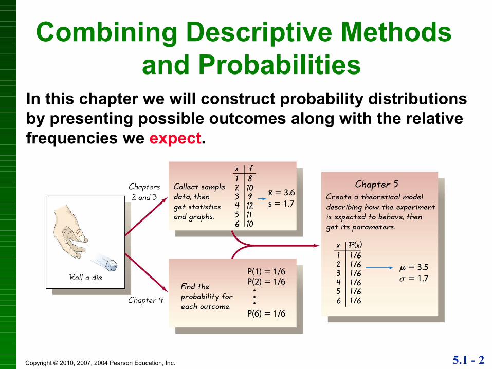
Combining Descriptive Methods and Probabilities

In this chapter we will construct probability distributions by presenting possible outcomes along with the relative frequencies we expect.

5.1 - 3Copyright © 2010, 2007, 2004 Pearson Education, Inc.

Random VariableProbability Distribution

Random variableIt is a variable (typically represented by X) that has a single numerical value, determined by chance, for each outcome of a procedure

Probability distributionIt gives the probability for each value of the random variable; often expressed in the format of a graph, table, or formula

5.1 - 4Copyright © 2010, 2007, 2004 Pearson Education, Inc.

Discrete and Continuous Random Variables

Discrete random variableeither a finite number of values or countable number of values, where “countable” refers to the fact that there might be infinitely many values, but they result from a counting process

Continuous random variableinfinitely many values, and those values can be associated with measurements on a continuous scale without gaps or interruptions →Chapter 6

5.1 - 5Copyright © 2010, 2007, 2004 Pearson Education, Inc.

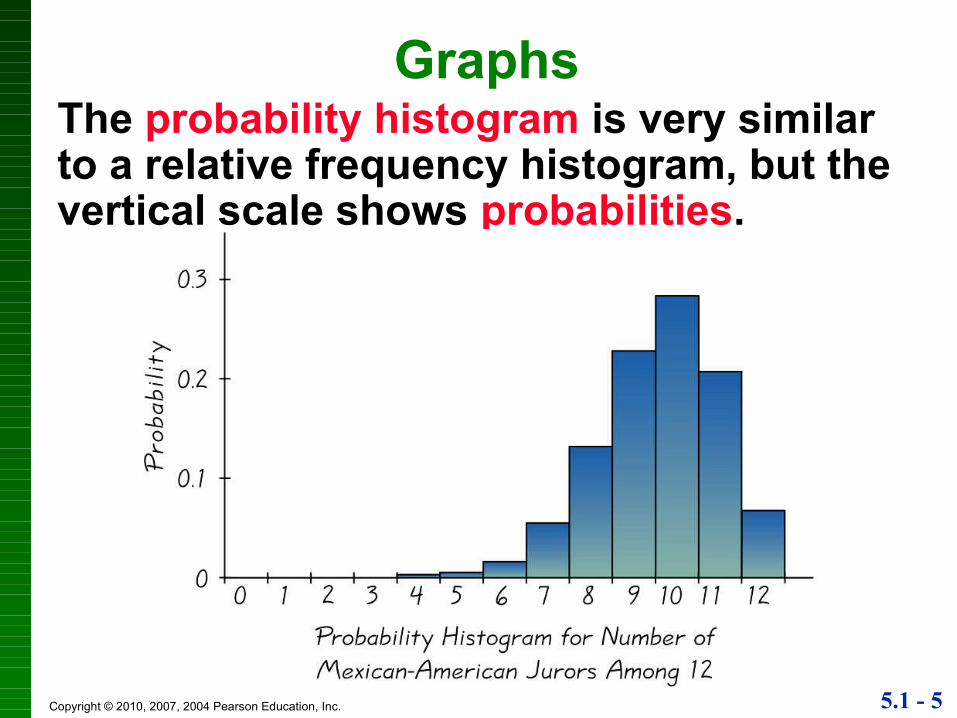
GraphsThe probability histogram is very similar to a relative frequency histogram, but the vertical scale shows probabilities.

5.1 - 6Copyright © 2010, 2007, 2004 Pearson Education, Inc.

Requirements for Probability Distribution

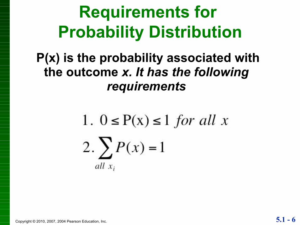
P(x) is the probability associated with the outcome x. It has the following

requirements

5.1 - 7Copyright © 2010, 2007, 2004 Pearson Education, Inc.

Expected Value

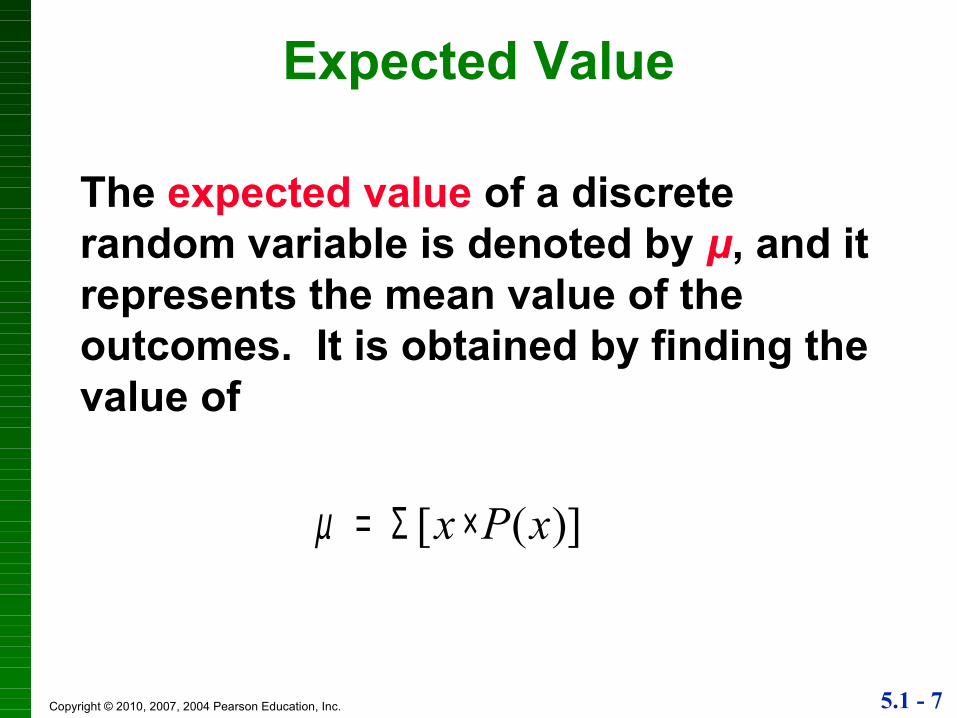
The expected value of a discrete random variable is denoted by μ, and it represents the mean value of the outcomes. It is obtained by finding the value of

[ ( )]x P xµ = Σ ×

5.1 - 8Copyright © 2010, 2007, 2004 Pearson Education, Inc.

Variance and Standard Deviation

The variance of a discrete random represents the variability of the outcomes. The square root of the variance is called the standard deviation.

2 2 2[( ( )]x P xσ µ= Σ × −

2 2[( ( )]x P xσ µ= Σ × −

2 2[( ) ( )]x P xσ µ= Σ − × Variance

Variance (shortcut)

Standard Deviation

5.1 - 9Copyright © 2010, 2007, 2004 Pearson Education, Inc.

Identifying Unusual ResultsProbabilities

Rare Event Rule for Inferential Statistics

If, under a given assumption (such as the assumption that a coin is fair), the probability of a particular observed event (such as “no more than one head in 10 tosses of a coin”) is extremely small, we conclude that the assumption is probably not correct.

5.1 - 10Copyright © 2010, 2007, 2004 Pearson Education, Inc.

Identifying Unusual ResultsProbabilities

Using Probabilities to Determine When Results Are Unusual Unusually high: x successes among n

trials is an unusually high number of successes if P(x or more) ≤ 0.05.

Unusually low: x successes among n trials is an unusually low number of successes if P(x or fewer) ≤ 0.05.

5.1 - 11Copyright © 2010, 2007, 2004 Pearson Education, Inc.

Identifying Unusual ResultsRange Rule of Thumb

According to the range rule of thumb, most values should lie within 2 standard deviations of the mean.We can therefore identify “unusual” values by determining if they lie outside these limits:

Maximum usual value =

Minimum usual value =

2µ σ+

2µ σ−

5.1 - 12Copyright © 2010, 2007, 2004 Pearson Education, Inc.

Section 5-3Binomial Probability

Distributions

5.1 - 13Copyright © 2010, 2007, 2004 Pearson Education, Inc.

Binomial ExperimentA binomial probability distribution results from a procedure that meets all the following requirements:1. The procedure has a fixed number of trials.2. The trials must be independent. (The outcome

of any individual trial doesn’t affect the probabilities in the other trials.)

3. Each trial must have all outcomes classified into two categories (commonly referred to as success and failure).

4. The probability of a success remains the same in all trials.

5.1 - 14Copyright © 2010, 2007, 2004 Pearson Education, Inc.

Notation for Binomial Probability Distributions

S and F (success and failure) denote the two possible categories of all outcomes; p and q will denote the probabilities of S and F, respectively, so

P(S) = p (p = probability of success)

P(F) = 1 – p = q (q = probability of failure)

5.1 - 15Copyright © 2010, 2007, 2004 Pearson Education, Inc.

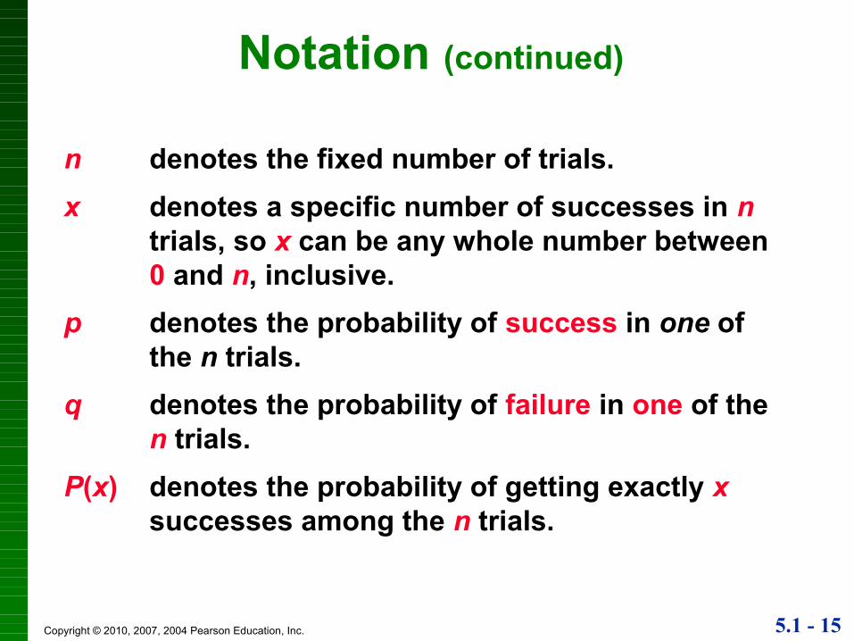
Notation (continued)

n denotes the fixed number of trials. x denotes a specific number of successes in n

trials, so x can be any whole number between 0 and n, inclusive.

p denotes the probability of success in one of the n trials.

q denotes the probability of failure in one of the n trials.

P(x) denotes the probability of getting exactly x successes among the n trials.

5.1 - 16Copyright © 2010, 2007, 2004 Pearson Education, Inc.

Method 1: Using the Binomial Probability Formula

where

n = number of trials

x = number of successes among n trials

p = probability of success in any one trial

q = probability of failure in any one trial (q = 1 – p)

)()1()!(!

!( xnx ppxnx

n ) successesxP −−−

=

5.1 - 17Copyright © 2010, 2007, 2004 Pearson Education, Inc.

Binomial Probability Formula

Number of outcomes with

exactly x successes

among n trials

The probability of x successes among n trials

for any one particular order

!( )( )! !

x n xnP x p qn x x

−= × ×−

5.1 - 18Copyright © 2010, 2007, 2004 Pearson Education, Inc.

Method 2: Using TechnologyExcel can all be used to find binomial probabilities.

=BINOMDIST(A1, 5, 0.75, 0)

5.1 - 19Copyright © 2010, 2007, 2004 Pearson Education, Inc.

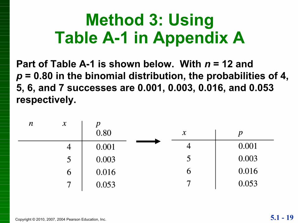
Method 3: UsingTable A-1 in Appendix A

Part of Table A-1 is shown below. With n = 12 and p = 0.80 in the binomial distribution, the probabilities of 4, 5, 6, and 7 successes are 0.001, 0.003, 0.016, and 0.053 respectively.

5.1 - 20Copyright © 2010, 2007, 2004 Pearson Education, Inc.

Section 5-4Mean, Variance, and Standard

Deviation for the Binomial Distribution

5.1 - 21Copyright © 2010, 2007, 2004 Pearson Education, Inc.

Binomial Distribution: Formulas

Where

n = number of fixed trials

p = probability of success in one of the n trials

q = probability of failure in one of the n trials

pnp

np

)1( −=

=

σ

µ

5.1 - 22Copyright © 2010, 2007, 2004 Pearson Education, Inc.

Interpretation of Results

Maximum usual values = Minimum usual values =

It is especially important to interpret results. The range rule of thumb suggests that values are unusual if they lie outside of these limits:

2µ σ+

2µ σ−