69

SECTION 6: CANOPY INSECTS

CANOPY ARTHROPODS AND BUTTERFLY SURVEY: PRELIMINARY REPORT

Allan D Watt1 and Paul Zborowski2

1Institute of Terrestrial Ecology, Edinburgh Research Station, Bush Estate, Penicuik, Midlothian EH26 0QB, Scotland, UK; 2PO Box 867, Kurunda, QLD 4872, Australia

6.1 Introduction: Arthropod diversity in tropical forests represents a concentration of biodiversity locally, regionally and globally. Arthropods carry out many significant ecosystem processes, notably decomposition, herbivory and pollination, and they also represent a food source for many vertebrate species. A few Lepidoptera are even a direct source of income in parts of Indonesia and elsewhere. Forest clearance, whether partial or complete, represents a major threat to arthropod diversity. The size of this threat is, however, unknown, as are the consequences for ecosystem 'health'. Theoretical predictions of species extinctions as a result of forest clearance are no substitute for direct measurement of biodiversity. Among the many problems with theoretical predictions based on supposed species-area relationships is the assumption that areas, once cleared of forest, are no longer suitable for any species. This is clearly untrue - secondary forest, plantations of rubber and other tree species and other types of land use all have the potential to contain many arthropods and other species. We are clearly correct in assuming that some forms of land use have lower levels of biodiversity than intact forest, but few studies have actually measured the effect of land-use change on biodiversity. The main problem with actually measuring biodiversity (and the attraction of theoretical approaches) is that biodiversity is impossible to measure in its entirety. Rapid biodiversity assessment methods have therefore been developed to allow comparisons of biodiversity in different places, or the same place at different times, by sampling a subset of biodiversity in a statistically rigorous way in as short a time as possible. The lowland forests of Sumatra have been logged and cleared to such an extent that very little intact forest remains. Clearance has resulted in a range of land uses including secondary forest, rubber plantations and Imperata grassland. The effect on biodiversity of such dramatic changes in land use is not known, and there is an urgent need to develop a rational strategy for the conservation of biodiversity. This strategy might entail the protection of remaining fragments of intact forest or the promotion of alternative land uses which are both productive and rich in biodiversity. Such a strategy requires a much better understanding of the variation in biodiversity in the mosaic of land uses in lowland Sumatra. As part of an overall programme to carry out a rapid biodiversity assessment in the Jambi Province of Sumatra, assessment of arthropod diversity was measured in several ways. This report describes canopy arthropod and butterfly surveys. Separate reports describe termite diversity assessment (Jones et al. 1988), light trapping and general insect survey. The aim of this part of the project was to assess the impact of logging and other land use changes on the diversity of arthropods in central Sumatra. Canopy arthropods were surveyed because previous studies indicate that arthropod diversity reaches a maximum in the canopies of tropical forest trees. However, few studies have compared the diversity of arthropods in the canopies of intact forest and plantation trees. Butterfly surveys were carried to provide a comparison of insect diversity in all sites -- several land-use types surveyed had no tree canopy.

70

The following land use types were surveyed: • Intact forest • Logged forest • Secondary forest • Jungle rubber • Rubber plantation • Paraserianthes plantation • Cassava fields • Chromolaena fallow • Imperata grassland

Full site descriptions are given by Gillison et al. (this report). 6.2 Aims and objectives: The aim of this project was to assess the impact of logging and other land use changes on the diversity of arthropods in central Sumatra and so provide baseline data for biodiversity assessment based on arthropod diversity. The objectives of this project were:

• To assess the abundance and diversity of the canopy arthropod community of selected land-use types.

• To assess the abundance and diversity of the butterfly community of selected land-use types.

6.3 Personnel: Allan D Watt - Institute of Terrestrial Ecology, Scotland, UK Paul Zborowski - Kuranda, Australia C Noor Rohmah - CIFOR, Indonesia 6.4 Methods: 6.4.1 Review of existing methods: 6.4.1.1 Introduction: A wide range of methods is used to assess the diversity of insects in tropical forests and other habitats. These include canopy fogging and butterfly transects; the two methods used here and discussed below. Other methods include a) general collecting, b) ground quadrat or transect sampling (as used to estimate termite and ant diversity (Jones et al.1988)), c) light trapping, and d) Malaise and flight interception trapping. These methods are discussed at length elsewhere and will not be described in detail here. It is worth pointing out that some methods are more suitable for collection of specimens for taxonomic work, and other methods are more suitable for biodiversity assessment. The key requirement for the latter is comparability. Many methods do not provide data that are comparable or are only comparable after analytical methods, which are not designed for biodiversity assessment (such as rarefaction). Broadly speaking, techniques which employ standardised sampling across transects or grids are the best methods and general collecting over non-standardised time periods are the worst. Trapping techniques should also be avoided where possible (at least in rapid surveys) because unless the

71

traps are used under the same environmental conditions (e.g. cloud cover and moonlight for light trapping), the results will not be comparable. Additional problems exist for 'passive' traps, such as Malaise traps, whose catches are affected by the degree to which they are located in open (e.g. grassland) or closed habitats (e.g. intact forest). This is a problem which may not be overcome, and results may be obtained which reflect the movement of insects within and through plots, rather than the diversity of insects within them. 6.4.1.2 Canopy arthropods: The sampling or canopy arthropods has only been made possible through the development of canopy fogging methods. A full review of canopy sampling is given by Stork, Adis and Didham (1995). The techniques as applied in this project are outlined below. 6.4.1.3 Butterfly sampling: A number of different approaches can be used to sample butterflies, including trapping and netting, but perhaps the most significant development in butterfly survey has been the use of 'butterfly walks' (Pollard and Yates 1993). This method was originally developed for European species and has proved useful in quantifying temporal and spatial trends in the abundance and diversity of species in the UK and elsewhere (e.g. Pollard, Moss and Yates 1995). It has now also been adapted for use in tropical forests (e.g. Hill et al. 1995, Watt et al. 1997, Lawton et al. 1998, Stork et al. in prep.). 6.4.2 Field methods used on this survey: 6.4.2.1 Plot locations: Two plots were chosen in each land-use type, apart from Chromolaena fallow and secondary forest (where single plots were surveyed). The plots in intact forest, logged forest and Paraserianthes plantation were distinct enough spatially to be regarded as replicates for the arthropod survey, but the rubber plantation, jungle rubber, Cassava and Imperata plots were situated very close to each other and should be regarded as 'psuedo-replicates'. The data from these plots have not been combined for the purposes of this report, but this problem is discussed below. 6.4.2.2 Canopy fogging: Canopy fogging was done at all 11 plots with tree canopies, i.e. the forest and plantation plots. A 'King' fogger [specifications available] was used to fog the canopy with a pyrethroid-based insecticide diluted with diesel. In each plot, apart from the jungle rubber plots, 25 1m2 collecting trays were suspended on ropes strung between trees. In each of the jungle rubber plots, 20 trays were used. The collecting trays were placed within, or close to, the 4×50 m transects used for the plant surveys (Gillison et al. 1988). Approximately two trays were placed under each tree so that about twelve trees were fogged in each plot. A collecting bottle was attached to each tray with approximately 2 cm of 70% alcohol. A pre-printed label was placed in each collecting bottle identifying the location of each sample. One hour after fogging, the trays were washed down with 70% alcohol and the collecting bottles (and trays) were removed. The arthropod samples were then cleaned, transferred to glass tubes and sorted as described below.

72

6.4.2.3 Butterfly transects: Butterfly transects were done in all plots, i.e. those with and without tree canopies. Two butterfly transects were sampled in each plot, so that each of the two available recorders could work independently without disturbance. Each transect comprised about half the ‘plant’ transects plus another 25m. The observers walked up and down their transect for 30 minutes and then moved to the other transect. Thus each plot was surveyed for two person-hours. The observers attempted to catch any butterfly flying close to them. Captured butterflies were placed in paper envelopes on which were written the date, time, plot number and recorder. Butterfly abundance in each plot was measured by additionally recording the number of butterflies seen and not caught. All butterflies were identified to family level in the field. Captured butterflies were removed for sorting to morpho-species. 6.4.3 Analysis: 6.4.3.1 Canopy fogging: Canopy fogging was used to assess the abundance of arthropods in different orders and the diversity of ants, spiders and beetles. Thus, during the field survey ants, beetles and spiders were removed from each sample, the samples were fully sorted to order, and the abundance of each group recorded. The aim of post-field survey work is to: 1. Sort the ants, beetles and spiders to morpho-species. 2. Sort all samples to order. For this report, preliminary analyses on the data were carried out as described in the results section. After sorting to morpho-species, further analyses were being carried out, including estimation of species richness (Colwell and Coddington and Coddington 1994) and comparison of the species composition of different sites (Krebs 1989). 6.4.3.2 Butterfly transects: It was concluded that there were insufficient individual butterflies caught, as a result of the time available for surveying butterflies, to allow comparisons of species richness and composition. Analysis of butterfly abundance, including the abundance of different families of butterflies was carried out. 6.4.4 Data storage and access: At present copies of all data are held by the consultants and CIFOR. Long-term arrangements for data storage and access will be made during early 1998. (Annex III, Table 8,9,10) 6.5 Preliminary results: 6.5.1 Canopy arthropod abundance: Total arthropod abundance The mean number of arthropods varied from about 20 to 290 arthropods m-2 (Figure 6.1). Arthropods were most abundant in one of the jungle rubber plots (BS11) and least abundant in

73

one of the Paraserianthes plots (BS6). Note that Figure 6.1 and subsequent figures show mean abundances and standard errors. Abundance of different arthropod groups Table 6.1 shows the average number of arthropods in each of the groups sorted to order (or family). Note that all the data discussed below are from partial sorting, apart from the ants, beetles and spiders, and must be considered to be preliminary. The most abundant groups were the ants and the termites, on average 32 and 21 m-2 , respectively. Together these two groups made up 67% of the total number of arthropods sampled. The next most abundant groups were the Coleoptera, Diptera, Hemiptera, Thysanoptera, and spiders (Araneae). Together these group, plus the ants and termites, made up 85% of the total number of arthropods. Psocoptera, Hymenoptera (other than ants), Collembola and several other groups made up the remaining 15%. Each group is considered separately below. Ants Not surprisingly, the pattern of abundance of ants in different plots was very similar to the pattern of abundance of total arthropods (Figure 6.2). Ants were notably abundant in the jungle rubber plots (BS11 in particular), one of the intact forest plots (BS1), and the secondary forest plot. Ants were notably few in numbers in the rubber plantation plots. Termites Termites were the most patchily distributed group across the different plots (Figure 6.3). They were only recorded in four plots and abundant in only two of those: one of the intact forests plots (BS2), and one of the logged forest plots (BS5).

Table 6.1 The mean and percentage abundance of different arthropod groups recorded from

canopy fogging at Pasir Mayang area, Jambi, Sumatra Nov. 1997.

Order Mean Percentage Ants 31.7 32.7 Termites 20.7 21.3 Coleoptera 8.3 8.6 Diptera 6.4 6.6 Hemiptera 5.5 5.7 Thysanoptera 5.2 5.4 Spiders 4.6 4.7 Psocoptera 4.4 4.5 Hymenoptera 3.5 3.6 Collembola 2.7 2.8 Lepidoptera 1.5 1.6 Acari 0.9 0.9 Orthoptera 0.8 0.8 Blatodea 0.5 0.6 Neuroptera 0.1 0.1 Total 97.0 100.0

74

Coleoptera Coleoptera were most abundant in the jungle rubber plots and one of the rubber plantation plots (Figure 6.4). Elsewhere, they were more-or-less equally abundant. Diptera Diptera were most abundant in the rubber plantation plots, the jungle rubber plots, one of the logged forest plots (BS5) and one of the Paraserianthes plots (BS7) (Figure 6.5). Hemiptera Hemiptera were more abundant in the logged and secondary forest plots, the jungle rubber plots and one of the Paraserianthes plots (BS7) than elsewhere (Figure 6.6). Thysanoptera Thysanoptera were particularly abundant in the jungle rubber plots and one of the logged forest plots (BS4) (Figure 6.7). Spiders Spiders were most abundant in one of the jungle rubber plots (BS11) and more or less evenly abundant elsewhere (Figure 6.8). Psocoptera Psocoptera were most abundant in one of the jungle rubber plots and least abundant in one of the Paraserianthes plots (BS7) (Figure 6.9). Hymenoptera Hymenoptera other than ants were notably abundant in one of the jungle rubber plots (BS11) and notably few in number in one of the Paraserianthes plots (BS6) and one of the intact forest plots (BS2) (Figure 6.10). Collembola Collembola were most abundant in the forest plots, recorded in low numbers in the jungle rubber and rubber plantation plots and absents from the Paraserianthes plots (Figure 6.11). Lepidoptera Lepidoptera were notably abundant in only one plot, the BS8 Paraserianthes plots (Figure 6.12). Acari Acari were more abundant in the secondary forest plot and one of the logged plots (BS4) than elsewhere (Figure 6.13). Orthoptera Orthoptera were uncommon in all plots, particularly the rubber plantation plots, and were not recorded in the Paraserianthes plots (Figure 6.14). Blattodea Small numbers of Blattodea were recorded but they were most abundant in the secondary forest plot and one of the jungle rubber plots (BS11) and not recorded in the Paraserianthes plots (Figure 6.15).

75

Neuroptera Very few Neuroptera were recorded in the survey, none at all in the jungle rubber and Paraserianthes plots (Figure 6.16). 6.5.2 Butterfly transects: 6.5.2.1 Total butterflies: The total number of butterflies caught or seen in an hour ranged from almost 50 in one of the rubber plantation plots to less than one in the Imperata grassland plots (Figure 6.17). Butterflies were particularly uncommon in the Imperata and Cassava plots and in one of intact forest plots (BS2), and most abundant in the jungle rubber, Chromolaena, one of the logged forest plots (BS4) and one of the rubber plantation plots (BS9). Figure 6.18 shows the numbers of butterflies seen; that is, it excludes the relatively small numbers of butterflies caught. It is included to show the variation between different sampling periods. The number of butterflies recorded in each family is described below. Papilionidae The greatest numbers of papilionids were recorded in the jungle rubber plots and one of the rubber plantation plots (BS9), and none were recorded in the Cassava and Imperata plots (Figure 6.19). Pieridae Large numbers of pierids were recorded in one of the rubber plantation plots (BS9), intermediate numbers were recorded in the jungle rubber plots and one of the logged forest plots (BS4), and few or none were recorded elsewhere (Figure 6.20). Nymphalidae Nyphalids were more abundant in the jungle rubber plots and the Chromolaena plot than elsewhere (Figure 6.21). Lycaenidae Lycaenids were more abundant in the jungle rubber, rubber plantation and one of the logged forest sites than elsewhere and notably absent from the Cassava, Imperata and one of the intact forest plots (BS2) (Figure 6.22). 6.6 Discussion: 6.6.1 Preliminary results: 6.6.1.1 Canopy fogging: It must be emphasised that the above results are preliminary, subject to amendment after the final order sorting and include no species diversity information. The following tentative observations should, however be highlighted as a basis for subsequent discussion. • Eleven plots were surveyed, producing a total of 22,700 arthropods, an average of 97m-2. • The most abundant groups were ants and termites. • The abundance and composition of arthropod taxa was affected by land use as follows:

• total arthropod abundance and the abundance of ants, Coleoptera, spiders, Hemiptera, Thysanoptera, Hymenoptera (other than ants) and Blattodea was greatest in the jungle

76

rubber plots; however, these plots contained relatively low numbers of Collembola, Acari and Neuroptera;

• the abundance of arthropods in the intact forest plots was surprisingly low but these plots, like all ‘forest’ plots, contained relatively high numbers of Collembola;

• arthropod numbers in the logged and secondary plots were greater than or similar to those found in the intact forest plots;

• total arthropod numbers were lowest in the plantation plots; the rubber plantation plots had particularly low numbers of ants, Collembola, Orthoptera and Blattodea and the Paraserianthes plots contained no Collembola, Orthoptera, Blattodea and Neuroptera.

In discussing these results, their unique nature must be borne in mind: no other study of the effects of land use on arthropod diversity has included such a range of land uses. Thus we can compare the results of this study with surveys of intact and disturbed forest elsewhere, but we cannot compare the jungle rubber and plantation plots with studies elsewhere, because this is the first time this has been attempted. Nevertheless:

• The mean total number of arthropods recorded in this survey is in line with that recorded elsewhere (e.g. Watt et al. (1997a) in Cameroon).

• The numbers of ants and other taxa accord with other studies, but the number of termites is markedly higher than found elsewhere.

• This study is similar to a few others (e.g. Eggleton et al. 1996, Watt et al. 1997ab, Lawton et al. 1998) in finding that the replacement of intact forest with other land uses tends to result in a decrease in the abundance of several groups of arthropods.

• This survey suggests that some land-use alternatives to intact forest, such as jungle rubber, may be rich in arthropods.

Differences in arthropod abundance do not necessarily lead to parallel differences in arthropod diversity so it must again be emphasised that these comments are tentative. 6.6.1.2 Butterfly survey: The butterfly survey suffered from being too rapid. Because of the priority given to canopy sampling in as many plots as possible, we were only able to spend a maximum of two person hours in each plot. This meant that the numbers of butterflies caught were too small to permit analysis, and we have relied instead on the numbers seen during the transect walks. Even these data are not as useful as they would have been if we had been able to spend about twice as long in each plot. There is also the concern that the numbers of butterflies were particularly low because of the recent drought. It would, therefore, be wrong to conclude too much from this survey. However the following tentative conclusions may be made:

• Butterfly abundance in most families was notably high in the jungle rubber plots. • The total number of butterflies in one of the rubber plantation plots was higher than

elsewhere, mainly due to the particularly high number of pierids recorded there. • Numbers of butterflies in one the intact forest plots was particularly low (lower than in

any of the other forest or plantation plots).

77

• The number of butterflies, particularly nymphalids, in the Chromolaena plot was surprisingly high. However, the proximity of this very small plot to the jungle rubber plots should be noted - these plots also had similar numbers of nymphalids.

• Very small numbers of butterflies were recorded in the Cassava and Imperata plots. 6.6.2 Review of methods: 6.6.2.1 Canopy fogging: Eleven sites were fogged and the material collected partially sorted in ten days (excluding time spent travelling and organising). Excluding sorting time (travel etc.), each plot took six whole days (or approximately 30 person days, comprising twelve person days of the consultant’s time, six person days from technical support staff and twelve person days from labourers). A total of about ten person days were spent partially sorting arthropods during and immediately after the survey. It is critically important that fogging surveys produce comparable data. This can only be guaranteed by the selection of representative plots and complete coverage of the canopy of each plot by the insecticide fog. We consider that all the plots chosen were representative of the land-use types in the survey area. We also consider that some plot types were more affected than others by the recent exceptional dry season. In particular, the intact forest plots and the Paraserianthes plots had much less canopy foliage than the rubber (jungle and plantation) plots. Most of the plot ‘pairs’ within each land use provided adequate replicates. However, the jungle rubber plots and the rubber plantation plots may have been too close to be considered true replicates for arthropod survey. The finding that there was marked variability in the abundance of arthropods in these plots demonstrates how spatially variable arthropod communities are in forests and plantations. 6.6.2.2 Butterfly survey: As mentioned above, insufficient time was given to the butterfly survey because of other priorities. Two (person) hours were spent collecting and recording the numbers of butterflies present in each plot. Surprisingly, this led to relatively little variation within the numbers of butterflies seen - note the errors in Figure 6.18. A relatively small increase in the amount of time spent recording butterfly abundance would have yielded much more useful data. Considerably more time would have been needed to collect useful data on species composition. The recent drought is likely to have reduced the number of butterflies in the area and this factor, plus the small amount of time spent surveying butterflies, means that we have probably considerably underestimated the abundance and diversity of butterflies in the study area. The comments above regarding replication apply to the butterfly survey as well. For example, many individual butterflies were seen flying from one plot to another in the rubber plantation. Plot size is likely to have affected the results in at least one case: the surprisingly numbers of butterflies recorded in the relatively small Chromolaena plot may have been dispersing from the nearby jungle rubber plots. 6.6.3 Relevance of study at regional and global levels: As mentioned above, no previous study has investigated the effects of such a range of land uses on arthropod diversity. It is therefore unique regionally and one of a very few similar studies globally (Eggleton et al., 1996; Watt et al., 1997; Lawton et al,. 1998).

78

6.6.4 Relevance to Rapid Biodiversity Assessment: This survey is relevant to Rapid Biodiverity Assessment (RBA) first, because arthropods comprise the largest component of terrestrial biodiversity. Second, the techniques employed fulfilled the criterion of 'rapid' because of the short time spent collecting samples in the field. Third, both methods were designed to produce comparable results. 6.6.5 Need for further surveys in this and other regions: Generally, many more surveys such as this are needed to assess the impact of land use change on biodiversity. These surveys should include as many land-use types as possible. For example, a similar survey in many other parts of Sumatra should include oil palm (not yet widely planted in the part of Jambi where this survey was conducted). Specifically, surveys such as this should be repeated where there is significant seasonal variation in the abundance of the taxa being considered or where particular conditions prevail. It is likely, for example, that this survey was affected by the severe drought which preceded it. 6.7 Conclusions: Tentative conclusions are presented above at the start of the Discussion section. The main conclusions are summarised below:

• This study is similar to a few others in finding that the replacement of intact forest with other land uses tends to result in a decrease in the abundance of several groups of canopy arthropods.

• However, this survey suggests that some land use alternatives to intact forest, such as jungle rubber, may be rich in canopy arthropods.

• The butterfly survey was of limited value apart from demonstrating that arthropod abundance and diversity in Cassava and Imperata was considerably poorer than in all other land use types.

6.8 Recommendations: It is recommended that:

• Further studies such as this are carried out to assess the impact of land use change on biodiversity.

• Such studies should use RBA techniques because it is more important to survey many land-use types adequately than a few sites in unnecessary detail.

• More research is therefore needed to establish suitable RBA techniques, particularly standard techniques for particular taxa.

• RBA projects should follow the multi-taxa approach adopted here (Gillison et al. 1998), so that as much biodiversity as possible is sampled without any assumptions being made about 'indicator' taxa, and so that relationships between the diversity of different taxa can be better understood and, perhaps, lead to the development of reliable biodiversity indicators.

79

6.9 References1

Colwell, R. K., and J. A. Coddington. (1994). Estimating terrestrial biodiversity through

extrapolation. Philosophical Transactions of the Royal Society of London Series B-Biological Sciences 345:101-118.

Eggleton, P., D. E. Bignell, W. A. Sands, N. A. Mawdsley, J. H. Lawton, and N. C. Bignell. (1996). The diversity, abundance and biomass of termites under differing levels of disturbance in the Mbalmayo Forest Reserve, southern Cameroon. Philosophical Transactions of the Royal Society of London Series B-Biological Sciences 351:51-68.

Gillison, A.N. (1988). A Plant Functional Attribute Proforma for Dynamic Vegetation Studies and Natural Resource Surveys. Tech. Mem. 88/3, CSIRO Div. Water Resources, Canberra.

Hill, J. K., K. C. Hamer, L. A. Lace, and W. M. T. Banham. (1995). Effects of selective logging on tropical forest butterflies on Buru, Indonesia. Journal Applied Ecology 32:754-760.

Krebs, C. J. (1989). Ecological Methodology, 1st Edition. Harper Collins, New York. Lawton, J. H., D. E. Bignell, B. Bolton, G. F. Bloemers, P. Eggleton, P. M. Hammond, M.

Hodda, R. D. Holt, T. B. Larsen, N. A. Mawdsley, N. E. Stork, D. S. Srivastava, and A. D. Watt. (1998). Biodiversity inventories, indicator taxa and effects of habitat modification in tropical forest. Nature 391:72-76.

Pollard, E., and T. J. Yates. (1993). Monitoring Butterflies for Ecology and Conservation. Chapman and Hall, London.

Pollard, E., D. Moss, and T. J. Yates. (1995). Population trends of common british butterflies at monitored sites. Journal Applied Ecology 32:9-16.

Stork, N., J. Adis, and R. K. Didham, editors. (1995). Canopy Arthropods. Chapman and Hall, London.

Watt, A. D., N. E. Stork, P. Eggleton, D. Srivastava, B. Bolton, T. B. Larsen, and M. J. D. Brendell. 1997a. Impact of forest loss and regeneration on insect abundance and diversity. Pp. 274-286 in A. D. Watt, N. E. Stork and M. D. Hunter, (eds.) Forests and Insects. Chapman and Hall, London.

Watt, A. D., N. E. Stork, C. McBeath, and G. L. Lawson. 1997b. Impact of forest management on insect abundance and damage in a lowland tropical forest in southern Cameroon. Journal Applied Ecology 34:985-998.

1References to other reports in this series to be inserted.

80

Intact, BS1

Intact, BS2

Logged, BS5

Logged, BS4

Secondary, BS3

Jungle rubber, BS10

Jungle rubber BS11

Rubber plant., BS8

Rubber plant., BS9

Paraserianthes, BS6

Paraserianthes, BS7

0

20

40

60

80

100

120

140

160

180

200

Num

ber p

er m

2

Ants

Intact, BS1

Intact, BS2

Logged, BS5

Logged, BS4

Secondary, BS3

Jungle rubber, BS10

Jungle rubber BS11

Rubber plant., BS8

Rubber plant., BS9

Paraserianthes, BS6

Paraserianthes, BS7

0

50

100

150

200

250

300

350

Num

ber p

er m

2Total arthropods

Figure 1 (above) and 2 (below): mean abundance of total arthropods and ants, respectively, assessed by canopy fogging in the Pasir Mayang area, Jambi, Sumatra, November 1997.

Figures 6.1. & 6.2

81

Intact, BS1

Intact, BS2

Logged, BS5

Logged, BS4

Secondary, BS3

Jungle rubber, BS10

Jungle rubber BS11

Rubber plant., BS8

Rubber plant., BS9

Paraserianthes, BS6

Paraserianthes, BS7

1

10

100

1000

Num

ber p

er m

2

Termites

Intact, BS1

Intact, BS2

Logged, BS5

Logged, BS4

Secondary, BS3

Jungle rubber, BS10

Jungle rubber BS11

Rubber plant., BS8

Rubber plant., BS9

Paraserianthes, BS6

Paraserianthes, BS7

0

5

10

15

20

25

30

35

Num

ber p

er m

2

Coleoptera

Figure 3 (above) and 4 (below): mean abundance of termites and Coleoptera, respectively, assessed by canopy fogging in the Pasir Mayang areJambi, Sumatra, November 1997.

Figures 6.3 & 6.4

82

Intact, BS1

Intact, BS2

Logged, BS5

Logged, BS4

Secondary, BS3

Jungle rubber, BS10

Jungle rubber BS11

Rubber plant., BS8

Rubber plant., BS9

Paraserianthes, BS6

Paraserianthes, BS7

0

2

4

6

8

10

12

14

16

Num

ber p

er m

2

Diptera

Intact, BS1

Intact, BS2

Logged, BS5

Logged, BS4

Secondary, BS3

Jungle rubber, BS10

Jungle rubber BS11

Rubber plant., BS8

Rubber plant., BS9

Paraserianthes, BS6

Paraserianthes, BS7

0

2

4

6

8

10

12

14

Num

ber p

er m

2

Hemiptera

Figure 5 (above) and 6 (below): mean abundance of Diptera and Hemiptera, respectively, assessed by canopy fogging in the Pasir Mayang areJambi, Sumatra, November 1997.

Figures 6.5 & 6.6

83

Intact, BS1

Intact, BS2

Logged, BS5

Logged, BS4

Secondary, BS3

Jungle rubber, BS10

Jungle rubber BS11

Rubber plant., B

S8

Rubber plant., B

S9

Paraserianthes, BS6

Paraserianthes, BS7

0

5

10

15

20

25

Num

ber p

er m

2

Thysanoptera

Intact, BS1

Intact, BS2

Logged, BS5

Logged, BS4

Secondary, BS3

Jungle rubber, B

S10

Jungle rubber B

S11

Rubber plant., B

S8

Rubber plant., BS9

Paraserianthes, BS6

Paraserianthes, BS7

Average0

2

4

6

8

10

12

14

16

Num

ber p

er m

2

Spiders

Figure 7 (above) and 8 (below): mean abundance of Thysanoptera and spiders, respectively, assessed by canopy fogging in the Pasir Mayang area, Jambi, Sumatra, November 1997.

Figures 6.7 & 6.8

84

Intact, BS1

Intact, BS2

Logged, BS5

Logged, BS4

Secondary, BS3

Jungle rubber, BS10

Jungle rubber BS11

Rubber plant., BS8

Rubber plant., BS9

Paraserianthes, BS6

Paraserianthes, BS7

0

2

4

6

8

10

12

14

Num

ber p

er m

2

Psocoptera

Intact, BS1

Intact, BS2

Logged, BS5

Logged, BS4

Secondary, BS3

Jungle rubber, BS10

Jungle rubber BS11

Rubber plant., BS8

Rubber plant., BS9

Paraserianthes, BS6

Paraserianthes, BS7

1

2

3

4

5

6

7

8

9

10

11

Num

ber p

er m

2

Hymenoptera

Figure 9 (above) and 10 (below): mean abundance of Psocoptera and Hymenoptera, respectively, assessed by canopy fogging in the Pasir Mayang area, Jambi, Sumatra, November 1997.

Figures 6.9 & 6.10

85

Intact, BS1

Intact, BS2

Logged, BS5

Logged, BS4

Secondary, BS3

Jungle rubber, BS10

Jungle rubber BS11

Rubber plant., BS8

Rubber plant., BS9

Paraserianthes, BS6

Paraserianthes, BS7

Intact, BS1

Intact, BS2

Logged, BS5

Logged, BS4

Secondary, BS3

Jungle rubber, BS10

Jungle rubber BS11

Rubber plant., BS8

Rubber plant., BS9

Paraserianthes, BS6

Paraserianthes, BS7

0

1

2

3

4

5

6

7

8

9

10

Num

ber p

er m

2

Collembola

Intact, BS1

Intact, BS2

Logged, BS5

Logged, BS4

Secondary, BS3

Jungle rubber, BS10

Jungle rubber BS11

Rubber plant., BS8

Rubber plant., BS9

Paraserianthes, BS6

Paraserianthes, BS7

Intact, BS1

Intact, BS2

Logged, BS5

Logged, BS4

Secondary, BS3

Jungle rubber, BS10

Jungle rubber BS11

Rubber plant., BS8

Rubber plant., BS9

Paraserianthes, BS6

Paraserianthes, BS7

0

1

2

3

4

5

6

7

Num

ber p

er m

2

Lepidoptera

Figure 11 (above) and 12 (below): mean abundance of Collembola and Lepidoptera, respectively, assessed by canopy fogging in the Pasir Mayang area, Jambi, Sumatra, November 1997.

Figures 6.11 & 6.12

86

Intact, BS1

Intact, BS2

Logged, BS5

Logged, BS4

Secondary, BS3

Jungle rubber, BS10

Jungle rubber BS11

Rubber plant., BS8

Rubber plant., BS9

Paraserianthes, BS6

Paraserianthes, BS7

Intact, BS1

Intact, BS2

Logged, BS5

Logged, BS4

Secondary, BS3

Jungle rubber, BS10

Jungle rubber BS11

Rubber plant., BS8

Rubber plant., BS9

Paraserianthes, BS6

Paraserianthes, BS7

0

0.5

1

1.5

2

2.5

3

3.5

4

Num

ber p

er m

2

Acari

Intact, BS1

Intact, BS2

Logged, BS5

Logged, BS4

Secondary, BS3

Jungle rubber, BS10

Jungle rubber BS11

Rubber plant., BS8

Rubber plant., BS9

Paraserianthes, BS6

Paraserianthes, BS7

Intact, BS1

Intact, BS2

Logged, BS5

Logged, BS4

Secondary, BS3

Jungle rubber, BS10

Jungle rubber BS11

Rubber plant., BS8

Rubber plant., BS9

Paraserianthes, BS6

Paraserianthes, BS7

0

0.5

1

1.5

2

2.5

3

Num

ber p

er m

2

Orthoptera

Figure 13 (above) and 14 (below): mean abundance of Acari and Orthoptera, respectively, assessed by canopy fogging in the Pasir Mayang area, Jambi, Sumatra, November 1997.

Figures 6.13 & 6.14

87

Intact, BS1

Intact, BS2

Logged, BS5

Logged, BS4

Secondary, BS3

Jungle rubber, BS10

Jungle rubber BS11

Rubber plant., BS8

Rubber plant., BS9

Paraserianthes, BS6

Paraserianthes, BS7

0

0.2

0.4

0.6

0.8

1

Num

ber p

er m

2

Neuroptera

Intact, BS1

Intact, BS2

Logged, BS5

Logged, BS4

Secondary, BS3

Jungle rubber, BS10

Jungle rubber BS11

Rubber plant., BS8

Rubber plant., BS9

Paraserianthes, BS6

Paraserianthes, BS7

Intact, BS1

Intact, BS2

Logged, BS5

Logged, BS4

Secondary, BS3

Jungle rubber, BS10

Jungle rubber BS11

Rubber plant., BS8

Rubber plant., BS9

Paraserianthes, BS6

Paraserianthes, BS7

0

0.5

1

1.5

2

2.5

3

3.5

Num

ber p

er m

2

Blattodea

Figure 15 (above) and 16 (below): mean abundance of Blatodea and Neuroptera, respectively, assessed by canopy fogging in the Pasir Mayang area, Jambi, Sumatra, November 1997.

Figures 6.15 & 6.17

88

Intact, BS1

Intact, BS2

Logged, BS5

Logged, BS4

Secondary, BS3

Jungle rubber, BS10

Jungle rubber BS11

Rubber plant., BS8

Rubber plant., BS9

Paraserianthes, BS6

Paraserianthes, BS7

Chromolaena, BS16

Cassava, BS14

Cassava, BS15

Impirata, BS12

Impirata, BS130

5

10

15

20

25

30

35

40

45

50

Num

ber p

er h

our

Total butterflies

Figure 17 (above) and 18 (below): mean abundance of butterflies seen and caught and seen only, respectively, assessed by transect counts in the Pasir Mayang area, Jambi, Sumatra, November 1997.

Intact, BS1

Intact, BS2

Logged, BS5

Logged, BS4

Secondary, BS3

Jungle rubber, BS10

Jungle rubber BS11

Rubber plant., BS8

Rubber plant., BS9

Paraserianthes, BS6

Paraserianthes, BS7

Chromolaena, BS16

Cassava, BS14

Cassava, BS15

Impirata, BS12

Impirata, BS13

Intact, BS1

Intact, BS2

Logged, BS5

Logged, BS4

Secondary, BS3

Jungle rubber, BS10

Jungle rubber BS11

Rubber plant., BS8

Rubber plant., BS9

Paraserianthes, BS6

Paraserianthes, BS7

Chromolaena, BS16

Cassava, BS14

Cassava, BS15

Impirata, BS12

Impirata, BS130

5

10

15

20

25

30

35

40

45

50

Num

ber p

er h

our

Total butterflies seen

Figures 6.17 & 6.18

89

Papilionids

Intact, BS1

Intact, BS2

Logged, BS5

Logged, BS4

Secondary, BS3

Jungle rubber, BS10

Jungle rubber BS11

Rubber plant., BS8

Rubber plant., BS9

Paraserianthes, BS6

Paraserianthes, BS7

Chromolaena, BS16

Cassava, BS14

Cassava, BS15

Impirata, BS12

Impirata, BS130

1

2

3

4

5

6

Num

ber p

er h

our

Intact, BS1

Intact, BS2

Logged, BS5

Logged, BS4

Secondary, BS3

Jungle rubber, BS10

Jungle rubber BS11

Rubber plant., BS8

Rubber plant., BS9

Paraserianthes, BS6

Paraserianthes, BS7

Chromolaena, BS16

Cassava, BS14

Cassava, BS15

Impirata, BS12

Impirata, BS130

5

10

15

20

25

30

35

Num

ber p

er h

our

Pierids

Figure 19 (above) and 20 (below): mean abundance of papilionids and pierids, respectively, assessed by transect counts in the Pasir Mayang area, Jambi, Sumatra, November 1997.

Figures 6.19 & 6.20

90

Intact, BS1

Intact, BS2

Logged, BS5

Logged, BS4

Secondary, BS3

Jungle rubber, BS10

Jungle rubber BS11

Rubber plant., BS8

Rubber plant., BS9

Paraserianthes, BS6

Paraserianthes, BS7

Chromolaena, BS16

Cassava, BS14

Cassava, BS15

Impirata, BS12

Impirata, BS130

5

10

15

20

25

Num

ber p

er h

our

Nymphalids

Figure 19 (above) and 20 (below): mean abundance of nymphalids and lycaenids, respectively, assessed by transect counts in the Pasir Mayang area, Jambi, Sumatra, November 1997.

Intact, BS1

Intact, BS2

Logged, BS5

Logged, BS4

Secondary, BS3

Jungle rubber, BS10

Jungle rubber BS11

Rubber plant., BS8

Rubber plant., BS9

Paraserianthes, BS6

Paraserianthes, BS7

Chromolaena, BS16

Cassava, BS14

Cassava, BS15

Impirata, BS12

Impirata, BS130

1

2

3

4

5

6

Num

ber p

er h

our

Intact, BS1

Intact, BS2

Logged, BS5

Logged, BS4

Secondary, BS3

Jungle rubber, BS10

Jungle rubber BS11

Rubber plant., BS8

Rubber plant., BS9

Paraserianthes, BS6

Paraserianthes, BS7

Chromolaena, BS16

Cassava, BS14

Cassava, BS15

Impirata, BS12

Impirata, BS130

1

2

3

4

5

6

Num

ber p

er h

our

0

1

2

3

4

5

6

Num

ber p

er h

our

0

1

2

3

4

5

6

Num

ber p

er h

our

Lycaenids

Figures 6.21 & 6.22

91

SECTION 7: SOIL MACROFAUNA

GROUND-DWELLING ANTS, TERMITES, OTHER MACROARTHROPODS AND

EARTHWORMS.

by D.E. Bignell1, E. Widodo1, F.X. Susilo2 and H. Suryo3 1Tropical Biology & Conservation Unit, University Malaysia Sabah, Kota Kinabalu, 2Lampung

University Faculty of Agriculture, Bandar Lampung, 3Gadjah Mada University Faculty of Forestry, Yogyakarta

7.1 Introduction: The Humid Forest Zones (HFZ) of the tropics cover about 8% of the Earth's land surface, of which about 20% occurs in SE Asia. The present forest is a mosaic of different types of land use: patches of logged-over forest in varying states of regrowth, secondary forest and fallow vegetation, some tree plantations including forms of agroforestry and significant remnants of primary vegetation, as well as degraded grasslands exhausted of almost all arable potential (Swift & Mutsaers, 1992; van Noordwijk et al., 1997). The dominant soils are acidic (oxisols and ultisols derived from low activity clays), commonly exhibiting Al toxicity, low cation-exchange capacity, low base saturation and low P availability. Consequently, they have low inherent fertility and, in many cases, low structural stability if soil organic matter is excessively depleted. The traditional food-production systems of the HFZ are those of shifting cultivation (slash and burn) and (increasingly) recurrent fallow rotation, with rice, plantain, cocoyam (Taro), maize, Cassava and groundnut as typical staples, the last two of these having relatively low fertility requirements. In recent years, socioeconomic factors (including changing world prices for cocoa, oil-palm, rubber latex and other cash crops), population growth, the restriction of urban employment opportunities and legal uncertainties over title to timber revenue, have led to an increase in the clearance of forest for food or cash-crop production and, concomitantly, an accelerated decline in the fertility of soils under cultivation as fallow periods have shortened (Woomer & Swift, 1994). Agricultural research for the HFZ has therefore been directed towards the improvement of sustainability, for example, by the conservation of soil organic matter and the provision of better mulching regimes. Added to this is the development of flexible mixed cropping systems, for example, the combination of marketable tree crops with field-planted staples, or mixtures of commercially valuable trees such as rubber and natural secondary regrowth (Scholes et al., 1994; van Noordwijk, 1997). Multistrata systems provide an opportunity for the simultaneous production of timber (and/or other tree crops) and food, with a sustained supply of organic matter and nutrients to soil and the stabilization of structure. The importance of macrofauna to the promotion of tropical soil fertility has been stressed in recent reviews (Fragoso et al.,1993; Lavelle et al.,1997; Garnier-Sillam & Harry, 1995; Nash and Whitford, 1995; Brussaard & Jumas,1996; Wood, 1996). The distribution, protection and stabilization of organic matter, the genesis of soil structure (macroaggregates), humification, the release of immobilized N and P, the improvement of drainage and aeration, and the increase in exchangeable cations have all been demonstrated in soils modified by termites and earthworms (e.g. Mulongoy & Bedoret, 1989; Lavelle et al.,1992; 1998). Soil ants and other macrofauna represent predators, herbivores (granivores) and bioturbators, bringing about important changes in the physical and chemical properties of soils, as well as dispersing plant propagules. Networks of galleries and chambers increase the porosity of the soil, increasing

92

drainage and aeration (Cherrett, 1989) and reducing bulk density (Baxter and Hole, 1967). Ant-plant communities are much more species-rich in the tropics than elsewhere; a pattern associated with habitat heterogeneity (Davidson and McKey, 1993; Folgarait, 1996). Depletion of termite abundance and diversity is now a well-established effect of forest clearance (Wood et al., 1982; Eggleton et al., 1995; 1996). Effects on earthworms also include the loss of typical forest species, but also possible invasion by exotic species, with adverse consequences for soil structure (Reddy & Dutta, 1984; Barros et al., 1996). Information on ants is limited, but Belshaw and Bolton (1994) found similar levels of leaf litter ant diversity in secondary forest, primary forest and cocoa plantations in Ghana. A more recent study in Cameroon by Watt et al. (1997), showed that moderate forest disturbance, for example, by enrichment planting after partial clearance, increased species numbers and overall ant abundance in both leaf-litter and canopy-dwelling ants. Complete clearance reduced abundance severely, although diversity was comparable to that in closed canopy forest. There is a general consensus that the conservation of indigenous invertebrate biodiversity should be an integral part of land-management strategies in the HFZ, if the goal of increased crop-yield sustainability (and concomitant forest conservation) is to be realized (e.g. Smith et al., 1993; Lavelle, 1996; Lavelle et al., 1998). The soil biota (and hence soils as a whole) respond to human-induced disturbance such as agricultural practices, deforestation, pollution and global environmental change with many negative consequences including loss of primary productivity, loss of cleansing potential for wastes and pollutants, disruption of global elemental cycles, feedbacks on greenhouse gas fluxes and erosion. At the same time, global food supply depends on intensive agriculture. As intensification proceeds, above-ground biodiversity is reduced, one consequence of which is that the biological regulation of soil processes is altered and often substituted by the use of mechanical tillage, chemical fertilizers and pesticides. This is assumed to reduce below-ground diversity as well, which, if accompanied by the extinction of species, may cause losses of function and reduce the ability of agricultural systems to withstand unexpected periods of stress and bring about undesirable effects. Scientists have begun to quantify the causal relationship between i) the composition, diversity and abundance of soil organisms, ii) sustained soil fertility, and iii) environmental effects such as greenhouse gas emission and soil carbon sequestration. Large numbers of farmers in the tropics have limited access to soil inputs (i.e. fertilizer and pesticides) but are nonetheless forced by circumstances to drastically reduce the complexity of their agroecosystems in an attempt to intensify production. An alternative solution is to intensify while at the same time retaining a greater degree of above-ground diversity. The maintenance of diversity of crops and other plants in cropping systems is widely accepted as a management practice which buffers farmers against short-term risk. Enhanced biodiversity and complexity above-ground contributes to the re-establishment or protection of the multiplicity of organisms below-ground able to carry out essential biological functions. This can be considered at both the field and the landscape level to enhance structural complexity and functional diversity, especially in degraded lands. In this paper, we report quantitative and qualitative sampling in 7 representative land uses in or close to the Pasir-Mayang Forest Reserve, Jambi Province, central Sumatra, using rapid assessment methods which enabled most sites to be examined in 1-2 days. Ants and other macrofauna were sampled qualitatively by the use of pitfall traps and quantitatively from standard soil monoliths.

93

7.2 Sites: The sites selected were chosen to have an approximately even spacing along a presumed disturbance gradient from pristine forest through to degraded grassland (Table 7.1). As a total of only 16 sites was available, not all land uses could be addressed, and no replication was attempted other than the within-site pseudo-replication inherent in transects and pitfall lines (see below). Sites were generally sampled last, in a planned sequence, after botanical, ornithological, soil and other site surveys had been completed and following the sampling of mammals, canopy arthropods and butterflies. Sampling was usually completed in 2 days, including dissection of monoliths. An intuitive grading of the sites, based on expected macrofaunal diversity, would be:

BS1 ---> BS3 ---> BS10 ---> BS8 ---> BS6 ---> BS14 ---> BS12 least disturbed most disturbed most diverse least diverse

The notional gradient used, reflecting disturbance history, disturbance intensity and vegetation is:

BS1---� BS3---� BS6---� BS8---�BS10 ---� BS12 ---� BS14

Table 7.1. Seven landuses selected for ant and other macrofaunal sampling in Pasir Mayang and

adjacent areas of central Sumatra.

Site coding

Dominant vegetation form General character GPS reference

BS 1 Intact rainforest A small area of pristine lowland forest on a moderately steep slope, well drained with closed stratified canopy and generally light understorey. Tree buttresses and stilts present.

01-04-47 S 102-06-02 E Pasir Mayang

BS 3 Secondary rainforest A ridge-top site contiguous with BS1 but logged-over with secondary regrowth on old log collection points and skid trails. Transects and pitfalls placed to run through secondary areas. Generally patchy canopy but of limited stratification. High liana/creeper burden.

01-04-43 S 102-05-55 E Pasir Mayang

94

Site coding

Dominant vegetation form General character GPS reference

BS 6 Young 3/4 yrs Paraserianthes plantation

A heavily disturbed site with line planted Sengon trees established after complete clearance. Canopy very open and the ground with a heavy load of dead wood.

01-05-59 S 102-06-43 E Pasir Mayang

BS 8 Rubber plantation A mature monospecific plantation in current production for latex, located on a gentle slope upper to ridge top. Canopy closure complete and herb/understorey layers very sparse. Large decaying tree trunks from previous forest clearance present with moderate dead wood load. About 15 yrs. old.

01-05-25 S 102-07-05 E Pasir Mayang

BS 10 Jungle rubber Mixture of old rubber trees still in production and secondary forest regrowth with high liana/creeper burden. About 25-30 yrs. old, at end of cycle ready for felling. Canopy closure ± complete and well stratified. Flat site, riverine.

01-10-12 S 102-06-50 E Pancuran Gading

BS 12 Imperata cylindrica Grassland: "alang-alang"

Large open ridge-top site devoid of trees with knee-high uniform stand of course grass. Little or no dead wood. Ground cracked and very hard.

01-36-05 S 102-21-22 E. Kuamang Kuning

BS 14 Cassava garden Open ridge-top site with line-planted Cassava, about 2 yrs old. Weeded to prevent growth of other vegetation. Ground very disturbed but little or no dead wood.

01-35-58 S 102-21-11 E Kuamang Kuning

An ordination of 16 sites, incorporating 9 land uses, based on 27 plant functional attributes and 3 canopy characters (height, cover and stem basal area) suggests the following sequence:

BS1 ---> BS3/BS10 ---> BS6 ---> BS8 ---> BS12 ---> BS14 most botanically diverse least botanically diverse (source A. Gillison, pers.comm.)

95

An expanded version of Table 1, incorporating botanical, soil physio-chemical data and additional site information is given as Annex III, Table 12.1. 7.3 Aims and objectives:

• To provide data on species richness, numerical density and biomass density for ground-

dwelling ants, with estimates of population variance for numerical density and biomass density, in 7 LUTs.

• To provide data on numerical density and biomass density of earthworms and termites, with estimates of population variance, in 7 land uses.

• To provide an estimate of species richness of earthworms. • To provide an estimate of taxonomic richness (to the best level of resolution possible)

for other macrofauna (in addition to earthworms, ants and termites). • To give pooled (i.e. overall) data for numerical density and biomass density for other

macrofauna. • To allocate basic functional attributes to macrofauna.

The objectives were developed to test the following hypotheses:

• Agricultural intensification results in a reduction of soil biodiversity, leading to a loss of

ecosystem services detrimental to sustained productivity. • Above-ground and below-ground biodiversity are interdependent across scales of

resolution from individual plant communities to the landscape. • Agricultural diversification (at several scales) promotes soil biodiversity and enhances

sustained productivity. • Sustainable agricultural production in tropical forest margins is significantly improved

by enhancement of soil biodiversity.

7.4 Methods: 7.4.1 Review of existing methods: General approaches to the sampling of invertebrate animals, and the advantages and disadvantages of particular methods, are descibed by Murphy (1962), Phillipson (1971) and Southwood (1978). Soils differ greatly in composition, particle size, structure, depth and compaction, and whether they are under trees, grassland or cultivation. Since the soil fauna is incorporated closely into the soil structure, the assessment of populations of these organisms is extremely difficult and laborious, and generally necessitates a wide range of specialized techniques if animals in the three major size categories (macrofauna, mesofauna and microfauna) are to be assessed (Edwards, 1991). The basic options are a) hand soil sifting and sorting (including litter layer dissection), b) trapping with or without baits, and c) extraction methods. In the last category are techniques based on flotation, which separates buoyant animals from the inert soil particles with water-based solutions (for example brine or sugar solutions) or organic solvents, or enables them to escape from the particle matrix by swimming (for example enchytraeids and nematodes in wet funnel methods), or dry heat extraction in which litter or soil samples suspended above funnels

96

are slowly dried, causing animals to migrate out of the litter into the funnels, from which they can be recovered, preserved and concentrated in alcohol (Bater, 1996). For ants, which are exceptionally mobile and respond rapidly to desiccation, a special modification of the extraction principle can be employed through the use of Winkler bags. These are narrow-mesh closed fabric bags forming a double-pyramid shape and enclosing suspended samples of soil or litter; the bags are hung up in a dry place for 6-8 days while the samples dry out naturally and any ants they contain are eventually captured in pots of alcohol fitted into the lower apex. However, extraction methods like this are generally slow and usually require some kind of laboratory base, so for rapid assessment focussed on the larger soil animals, it is normally sufficient to use just hand sorting; i.e. a measured quantity of soil or litter (usually delimited by a quadrat) is gradually crumbled over a sheet of plastic or other material and the invertebrates collected with forceps or pooter as they are released and stored in a suitable preservative (5% formalin for earthworms and gastropods; 70% alcohol for other invertebrates). Samples tend to accumulate faster than they can be sorted, so it is permissible to store samples in plastic bags (but out of direct sunlight) for up to 12 hours for later sorting. The efficiency of hand-sorting is generally high for animals which can be seen with the naked eye, as long as field assistants are adequately trained, but some authors have reported making allowances of up to 12% for lost or undiscovered specimens (e.g. Wood et al., 1982). Trapping methods can be used to exploit accidental encounter by invertebrates, but baiting is not usually employed for ants, as attractants may introduce bias by selecting for some species more than others. Pitfall traps, containers sunk into the soil flush with the soil surface, containing either a preservative or some other immobilizing fluid and with raised covers to prevent flooding by rain, are probably the most commonly used method of catching invertebrates (Bater, 1996). The main variations are in the size of container and the use, or otherwise, of guiding fins or other corralling devices to increase interception. The limitations of pitfall traps are largely in the interpretation of data, since the numbers of animals trapped are related both to overall numbers present and their activity, and so may not sample each population entirely. There is a tendency for such traps to accumulate ants, beetles, crickets, isopods, myriapods and spiders (all of which are active on the surface of the ground, particularly at night). The optimum period for capture is about 24 hours, after which traps are often disturbed by vertebtrates and birds. There are methods available to convert the numbers of invertebrates trapped to populations, usually based on physically delimiting sampling areas with some form of barrier or using mark-recapture techniques. 7.4.2 Functional classification of soil fauna: (after Lavelle, 1988; Anderson and Ingram, 1993). Soil invertebrates can be classified according to their feeding habits and distribution in the soil profile as follows: Epigeic species which live and feed on the soil surface. These may act as litter transformers or the predators of litter transformers, but do not actively redistribute plant material. Anecic species which remove litter from the soil surface through their feeding, redistributing it to other horizons or locations, accompanied by effects on soil structure and hydraulic properties.

97

Endogeic species which live entirely within the soil, feeding on organic matter and dead root materials, which are mixed with other components of the soil, creating mineral-humus complexes and influencing a large suite of soil properties. The quantification of these effects on soil processes requires detailed study, but a simple characterization of macrofauna can assist in assessing their role in different landuses and under various regimes of management (Table 7.2).

Table 7.2

Functional classification of common soil fauna Taxon Category Ants Epigeic and anecic Arachnids (esp. spiders) Epigeic Beetle adults Epigeic and endogeic Beetle larvae Epigeic Cockroaches Epigeic Centipedes Epigeic Cicada larvae Endogeic Crickets Epigeic Earthworms (pigmented) Epigeic and anecic Earthworms (unpigmented) Endogeic Millipedes Epigeic Slugs and snails Epigeic Wood-feeding termites Epigeic and anecic Soil-feeding termites Endogeic Fungus-growing termites Anecic Woodlice Epigeic

7.4.3 Sampling design: Sampling in each land use is based on a single quadrat of 40x5 m, which is compatible with concurrent botanical and other pedological sampling exercises (Gillison and Liswanti, this volume). The recommendation is for a minimum of 5 soil monoliths, each 25x25x30cm spaced along the mid-line of the transect at approximately 8m intervals, accompanied by at least 10 pitfalls (using 14cm diameter glass or plastic containers) arranged in a flanking line parallel to the transect or along its long edge. The choice of the starting point for the transect should be random, but its direction is normally determined by the line of best visual habitat homogeneity. 7.4.4 Procedure: Procedures follow Anderson and Ingram (1993) closely:

a. 5 sampling points (for monoliths) are located and marked within the transect.

b. 10 pitfall traps are fitted at roughly 4m intervals along one flank of the transect. The

traps are put in during the afternoon or early evening and emptied 24 hours later. Each trap contains a little water, with a few drops of detergent added, to immobilize specimens by drowning.

98

c. At each sampling point litter is removed from within a 25cm quadrat and hand-sorted at the site.

d. Isolate the monolith by cutting down with a spade a few centimetres outside the

quadrat and then digging a 20cm wide and 30cm deep trench around it. NB. In a variant of the method not adopted in Pasir Mayang, all invertebrates longer than 10cm excavated from the trench are collected; these will be mainly large millipedes and earthworms with very low population densities but representing an important biomass. Their abundance and biomass can be calulated on the basis of 0.42 m2 samples, i.e. the width of the block plus two trench widths, squared.

e. Divide the delimited monolith block into three layers, 0-10cm, 10-20cm and 20-

30cm. This can be done conveniently using a parang or machete held horizontally and grasped at both ends. Hand-sort each layer separately. If time is short or the light poor (sorting in closed canopy forest is usually difficult after about 3.30pm), bag the soil and remove to a laboratory. Ants can be extracted by gently brushing small (handful) quantities of soil through a course (5mm) sieve into a tray: the sieve retains the ants.

f. Record the number and fresh (preserved, after blotting) weight of all animals and

identify to at least the taxonomic and functional levels indicated in Table 7.2 (but preferably further). The presence and weight of termite fungus combs (if any) should also be noted.

7.4.5 Analysis: The following steps should be followed: i) Make a list of species, if possible grouped into subfamilies or families. Use generic names to generate alphabetical orders. Use the results from pitfall traps and monoliths to compile this list. Fully identified species should be listed with the full binomial and descriptive authority: e.g. Dorylus laevigatus Smith Morphospecies should be listed by number: e.g. Crematogaster sp. 1 Crematogaster sp. 2

......... etc. Species identified only to genus should be listed without numbers: e.g. Colobobsis sp. Incorporate the species list into a table showing the sites where each occurred. ii) Estimate abundance as numbers m-2 from each monolith (multiply the raw number per monolith by 16 (except earthworms and millipedes, see above), combining data for all species.

99

Calculate an arithmetical mean. To estimate the 95% confidence limits the primary data should be transformed as log10(x+1). If there are not too many zeros, this should roughly normalize the data and produce homogeneous variances from group to group. In difficult cases, a log-log transformation can be tried. Apply descriptive statistics to the transformed dataset, including 95% confidence limits, and back transform to obtain a geometric mean. Quote means for untransformed data, together with the geometric mean and confidence limits for log(x+1) transformed data. The transformed data can be used for histograms and site-to-site comparisons. Estimate biomass as g m-2 in a similar way. Use fresh weight or the mass of blotted preserved specimen, if possible. Avoid the use of dry weight because of the different oven temperatures used by different scientists and the variable water content of different types of organism. Where insect specimens in a range of sizes are available, an alternative method is to calibrate live biomass against head width in representative specimens covering the whole size range. The weight of unknowns can then be estimated from the curve. For log transformations of data, it is most convenient to work in (mg + 1), then back-transform and express as g. iii) Results should be presented as species/taxa lists, plus the standard histograms as illustrated below:

Figure 7.1. Graphical summaries of biodiversity data – some examples

100

Landuse systems

A B C D E

1000

2000

3000

0

10

20

30

Numerical density Biomass density

= geometric mean and 95%confidence limits, back-transformed

0

1

2

0

10

20

DIVERSITY

100

50

OTHERS

ANTS

EARTHWORMS

TERMITES

RELATIVE ABUNDANCE (for example):

EPIGEIC

ANECIC

ENDOGEIC

50

FUNCTIONAL GROUPABUNDANCE (for example):

100

iv) An overall quantitative synthesis of data for macrofauna can be attempted using the following matrix:

Table 7.3 Synthesis matrix for macrofauna

Region Landuse System A = natural

control site B C D E

e.g. Pasir Mayang x = 80 x = 67 x = 50 x = 95 x = 57 p = 0.1 p = 0.04 p = 0.11 p = 0.05 % = -16 % = -38 % = +19 % = -29

where, x = average of monoliths p = level of significance for a comparison with the control site by an appropriate

statistical test. % = percentage difference between the mean of each landuse and the control site, with

an indication (+/-) of the direction of change (increase or decrease). The control site is selected as the least disturbed local land use; in most cases this would be a tropical forest, preferably primary, or else old growth secondary or disturbed primary forest. Arrangement of sites in rank order to form a disturbance gradient may be somewhat arbitrary, especially if site histories are incompletely known, but disturbance intensity, management intensity and time since the imposition of disturbance are the usual criteria employed. Matrices can be prepared for the following data:

• total numerical density • total biomass density • earthworm numerical density • earthworm biomass density • earthworm species richness • termite numerical density • termite biomass density • termite species richness • ant numerical density • ant biomass density • ant species richness • all macroarthropod numerical density • all macroarthropod biomass density

v) A qualitative synthesis can be given by answering the following questions:

• what is the effect of each landuse system on biodiversity? • which groups change the most with disturbance and along the land use gradient? • what is the relationship between the functional group changes and the degree of

sustainability of each land use?

101

7.4.6 Data analysis: Carry out a non-parametric ANOVA (Kruskal-Wallis) on each dataset to see if there is a significant difference across the sites (or treatments). This can be followed by pairwise comparisons between sites using the Mann-Whitney U test. Parametric ANOVA can be performed on log transformed data. 7.5 Results: 7.5.1. Ants:

The total number of subfamilies sampled was 8: • Dorylinae: BS10 only • Formicinae: all sites • Myrmecinae: all sites • Ponerinae: all sites except BS14 • Leptanillidae: BS 8 only • Pseudomyrmicinae: BS 6 and BS 10 only • Cerapachyinae: BS 8 only • Dolichoderinae: BS 6, BS 10, BS 12 and BS 14 only

The species lists for each site are available in Annex III, Table 12.11 . Details of ant numerical density and biomass density by site and by stratum are given in Annex III, Table 12.2 and 12.3 , respectively. The following figures summarize ant diversity and abundance:

102

30

20

10

Figure 7.3. Ant abundance and biomass

Landuse systems

BS1 BS6 BS8 BS10 BS12

1000

7000

0

0.5

1.0

1.5

Numerical density Biomass density

= geometric mean and 95%confidence limits, back-transformed

500

BS3 BS14

Figure 7.2. Ant species richness

BS1 BS3 BS6 BS8 BS10 BS12 BS14

16 18

24

16

33

15

9

Abundance and biomass were totalled for each monolith and assessed by the non-parametric one-way Kruskal-Wallis ANOVA, using arithmetic data. Abundance and biomass did not vary significantly across the sites (p>0.05)). One-tailed pairwise comparisons of ant abundance between sites were, however, carried out by the Mann-Whitney test (Table 7.10). These generally showed significant differences between some of the richer sites (BS3, BS6, BS10) and those that were highly disturbed (BS12, BS14). BS3, BS6 and BS10 all had more ants than either BS12 or BS14 (p<0.025 in all comparisons). BS10 had more ants than BS 8 (p<0.025). All other site comparisons were non-significant (see Table 7.10 and Annex III, Table 12.10).

103

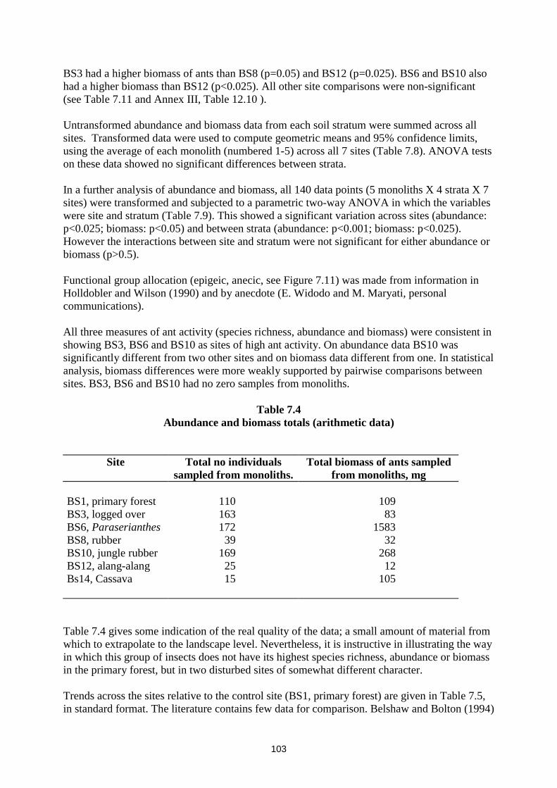
BS3 had a higher biomass of ants than BS8 (p=0.05) and BS12 (p=0.025). BS6 and BS10 also had a higher biomass than BS12 (p<0.025). All other site comparisons were non-significant (see Table 7.11 and Annex III, Table 12.10 ). Untransformed abundance and biomass data from each soil stratum were summed across all sites. Transformed data were used to compute geometric means and 95% confidence limits, using the average of each monolith (numbered 1-5) across all 7 sites (Table 7.8). ANOVA tests on these data showed no significant differences between strata. In a further analysis of abundance and biomass, all 140 data points (5 monoliths X 4 strata X 7 sites) were transformed and subjected to a parametric two-way ANOVA in which the variables were site and stratum (Table 7.9). This showed a significant variation across sites (abundance: p<0.025; biomass: p<0.05) and between strata (abundance: p<0.001; biomass: p<0.025). However the interactions between site and stratum were not significant for either abundance or biomass (p>0.5). Functional group allocation (epigeic, anecic, see Figure 7.11) was made from information in Holldobler and Wilson (1990) and by anecdote (E. Widodo and M. Maryati, personal communications). All three measures of ant activity (species richness, abundance and biomass) were consistent in showing BS3, BS6 and BS10 as sites of high ant activity. On abundance data BS10 was significantly different from two other sites and on biomass data different from one. In statistical analysis, biomass differences were more weakly supported by pairwise comparisons between sites. BS3, BS6 and BS10 had no zero samples from monoliths.

Table 7.4 Abundance and biomass totals (arithmetic data)

Site Total no individuals sampled from monoliths.

Total biomass of ants sampled from monoliths, mg

BS1, primary forest 110 109 BS3, logged over 163 83 BS6, Paraserianthes 172 1583 BS8, rubber 39 32 BS10, jungle rubber 169 268 BS12, alang-alang 25 12 Bs14, Cassava 15 105

Table 7.4 gives some indication of the real quality of the data; a small amount of material from which to extrapolate to the landscape level. Nevertheless, it is instructive in illustrating the way in which this group of insects does not have its highest species richness, abundance or biomass in the primary forest, but in two disturbed sites of somewhat different character. Trends across the sites relative to the control site (BS1, primary forest) are given in Table 7.5, in standard format. The literature contains few data for comparison. Belshaw and Bolton (1994)

104

give average litter-ant abundance across several woodland sites in Ghana as 117 m-2. Watt et al. (1997) examined a range of forest sites in Cameroon representing a disturbance gradient similar to that observed in Pasir Mayang, but give figures in the range 20-80 m-2. However, the lightly and heavily disturbed sites were towards the lower end of this range, while sites with intermediate disturbance yielded the higher abundances. Stork and Brendell (1993) give 3 g m-2 as the biomass of all non-social insects in the forest system of Seram, Indonesia.

Table 7.5 Trends across the sites relatives to the control sites (BS1)

Landuse System

Parameter Natural controlsite = BS1

BS1 BS6 BS8 BS10 BS12 BS14

Numerical density

Arithmetical average of monoliths, nos m-2

352 522 550 134 541 80 48

p value for comparison with control site (transformed data)

0 ns. ns. ns. ns. ns. ns.

% difference of means from control site

0 +48% +56% -62% +54% -77% -86%

Biomass density

Arithmetical average of monoliths, nos m-2

0.346 0.285 4.889 0.102 0.857 0.03 0.336

p value for comparison with control site (transformed data)

0 ns. ns. ns. ns. ns. ns.

% difference of means from control site

0 -18% +1400%

-71% +248%

-92% -1%

ns. = not significant (p > 0.05) 7.5.2. Termites: The species lists for each site are available in Section 8 of this report. Details of termite numerical density and biomass density by site and by stratum are given in Annex III, Table 12.4 and 12.5 , respectively. Figures 7.4 and 7.5 summarize termite diversity and abundance. Abundance and biomass were totalled for each monolith and assessed by the non-parametric one-way Kruskal-Wallis ANOVA, using arithmetic data. Abundance and biomass were found to vary significantly across the sites (Tables 7.9; p<0.025). One-tailed pairwise comparisons of ant abundance between sites were carried out by the Mann-Whitney test (Tables 7.10 and 7.11).

105

These generally showed significant differences between the richest site (intact rainforest, BS1) and others. In addition, sites BS3 and BS6 were significantly greater in abundance and biomass than site BS12 (the Imperata grassland; p varies between <0.05 and <0.005). There were no other significant differences between sites. Untransformed abundance and biomass data from each soil stratum were summed across all sites. Transformed data were used to compute geometric means and 95% confidence limits, using the average of each monolith (numbered 1-5) across all 7 sites (Table 7.8). ANOVA tests on these data showed that vertical biomass distribution varied significantly across the sites (Table 7.9; p<0.05). For both abundance and biomass, all 140 data points (5 monoliths X 4 strata X 7 sites) were transformed and subjected to a parametric two-way ANOVA in which the variables were site and stratum. This showed a significant variation across sites (p<0.001) and between strata (p<0.001). The interactions between site and stratum were significant for abundance (p<0.05) and biomass (p<0.01). Termites generally showed highest numerical and biomass densities in the top 10 cm of the soil. Functional group allocation (anecic, endogeic, see Figure 7.11) was made from knowledge of termite natural history (see Jones, 1999 in preparation). Generally, species nesting arboreally and feeding on the surface were designated anecic, those building epigeal nests and subterranean nests but feeding on the surface anecic, and those feeding within the soil endogeic, wherever the nesting site. The epigeic category was not recognized for termites. Overall, termite abundance and biomass were heavily reduced by forest disturbance. This confirms their status as sensitive indicators of forest quality (Eggleton et al., 1995; 1996; Watt et al. 1997). Diversity remained relatively high in two disturbed sites (BS3, logged over forest; BS10, jungle rubber), but this was not matched by a corresponding retention of abundance and biomass.

106

30

20

10

Figure 7.5. Termite abundance and biomass

Landuse systems

BS1 BS6 BS8 BS10 BS12

1000

3000

0

2.0

4.0

6.0

Numerical density Biomass density

= geometric mean and 95%confidence limits, back-transformed

500

BS3 BS14

Figure 7.4. Termite species richness

BS1 BS3 BS6 BS8 BS10 BS12 BS14

30

21

10

14

21

2 1

8.0

7.5.3. All macroarthropods: Macroarthropods other than ants and termites were recovered from monolith dissections and pitfall traps. These were predominantly Coleoptera, Diptera, Hemiptera, Dictyoptera Orthoptera, Isopoda, Myriapoda and Arachnida, including many juvenile forms. In most, cases identification was made at class and ordinal level only, more rarely to family, but abundance and biomass were determined as for ants and termites. To make use of the resulting data, they were added to those of ants and termites to make a composite dataset respresenting all macroarthropods. This is summarized in Figs. 7.6 and 7.7 below, with detailed information in Annex III, Table 12.6 and 12.7.

107

60

40

20

Figure 7.7. All macroarthropods abundance and biomass

Landuse systems

BS1 BS6 BS8 BS10 BS12

2000

6000

0

5

10

15

Numerical density Biomass density

= geometric mean and 95%confidence limits, back-transformed

1000

BS3 BS14

Figure 7.6. All macroarthropods taxonomic richness

BS1 BS3 BS6 BS8 BS10 BS12 BS14

5246

40 37

60

23

5

Diversity score = ant species + termite species + other groups at ordinal level or above(earthworms not included)

A crude diversity index for macroarthropods was obtained by summing ant and termite species richness, then adding other groups at the level of taxonomic resolution obtained. This shows a more even decline across the gradient, with the exception of BS10 (jungle rubber), which scored a higher diversity than any other site. However, it must be borne in mind that groups with inherent very high diversity, e.g. Coleoptera, Diptera, Arachnida, are almost certainly inaccurately represented (i.e. underestimated) by this method. Abundance and biomass were totalled for each monolith and assessed by the non-parametric one-way Kruskal-Wallis ANOVA, using arithmetic data. Abundance and biomass were found to vary significantly across the sites (Tables 7.9; abundance, p<0.005; biomass, p<0.025). One-tailed pairwise comparisons of ant abundance between sites were carried out by the Mann-Whitney test (Tables 7.10 and 7.11). For abundance, these generally showed significant differences between the richest site (intact rainforest, BS1) and others. In addition, sites BS6, BS8 and BS10 were significantly greater in abundance and biomass than heavily degraded sites

108

(BS12 and BS14; p varies <0.025 to <0.005,except BS6 vs BS14, which is not significant). For biomass, BS1 was significantly greater than BS3, BS12 and BS14. Biomass in BS12 and BS14 was also exceeded by that in BS10 and that in BS12 by BS6 and BS8. Untransformed abundance and biomass data from each soil stratum were summed across all sites. Transformed data were used to compute geometric means and 95% confidence limit,s using the average of each monolith (numbered 1-5) across all 7 sites (Table 7.8). ANOVA tests on these data showed that vertical abundance and biomass distribution varied significantly across the sites (Table 7.9; abundance, p<0.01; biomass, p<0.005). For both abundance and biomass, all 140 data points (5 monoliths X 4 strata X 7 sites) were transformed and subjected to a parametric two-way ANOVA in which the variables were site and stratum. This showed a significant variation across sites (p<0.001) and between strata (p<0.001). The interactions between site and stratum were not significant. The data are, of course, heavily influenced by ant and termite distributions, but for macroarthropods as a whole, the highest numerical and biomass densities were found in the top 10 cm of the soil. Functional group allocations for macroarthropods other than ants and termites (engineers, litter transformers, macropredators, see Figure 7.10 and epigeic, anecic, endogeic, see Figure 7.11) were made from knowledge of natural history and by reference to Anderson and Ingram (1993; Table 7.2). Animals which did not fit any of these categories, for example sap-feeders, were excluded from the subsequent analysis of functional group distribution across sites. Few, if any, published studies of soil macroarthropod communities are available for comparison with these data. The inclusion of data for arthropods other than ants and termites appears useful in providing some additional resolution between sites, not obtained from scrutiny of the ants and termites alone. This may be a consequence of the well-known patchiness of soil animal distributions, since individual groups may show very large variance between replicate samples in a single site,but a composite category of macroarthropods may show less overall variation. The category “macroarthropods”, however, disguises group to group turnovers which may characterize disturbance gradients. 7.5.4. Earthworms: Earthworms were recovered from monolith dissections, but were only rarely present in pitfall traps. Summary data on diversity, abundance and biomass are given in Figs. 7.8 and 7.9, with further details in Appendices 7.8 and 7.9. Overall earthworm diversity was low, with only a single morphospecies recognized from the forested BS1 and BS3 sites. However, very high abundance and biomass were associated with sites BS6 and BS10. Abundance and biomass were totalled for each monolith and assessed by the non-parametric one-way Kruskal-Wallis ANOVA, using arithmetic data. Abundance and biomass were found to vary significantly across the sites (Tables 7.9; p<0.005). One-tailed pairwise comparisons of ant abundance between sites were carried out by the Mann-Whitney test (Tables 7.10 and 7.11). For abundance, these showed significant differences between the richest site (jungle rubber, BS10; p<0.005) and all others. In addition, site BS6 was significantly greater than BS1, BS3, BS8 and BS12. BS14 (Cassava garden) was relatively abundant, exceeding BS1 and BS3 (p<0.025). For biomass, BS10 exceeded BS8 and BS12 (p variable <0.05 to <0.005), while BS6 exceeded BS1, BS3, BS8, BS12 and BS14. (p variable <0.05 to <0.005). This somewhat anomalous result reflects the large confidence interval associated with site BS10.

109

Untransformed abundance and biomass data from each soil stratum were summed across all sites. Transformed data were used to compute geometric means and 95% confidence limits, using the average of each monolith (numbered 1-5) across all 7 sites (Table 7.8). ANOVA tests on these data showed that vertical abundance and biomass distribution varied significantly across the sites (Table 7.9; p<0.001). For both abundance and biomass, all 140 data points (5 monoliths X 4 strata X 7 sites) were transformed and subjected to a parametric two-way ANOVA in which the variables were site and stratum. This showed a significant variation across sites (p<0.001.) and between strata (p<.001). The interactions between site and stratum were significant for both abundance (p<0.001) and biomass (p<0.001). Earthworms generally showed highest numerical and biomass demsities in the top 10 cm of the soil, with only a few specimens recovered below this level and none in the litter. Functional group allocation (epigeic, anecic, endogeic, see Figure 7.11) was made from pigmentation (see Lavelle, 1988 and Lavelle et al., 1997). Anecic and endogeic earthworms were considered engineers.

110

200

400

6

4

2

Figure 7.9. Earthworms abundance and biomass

Landuse systems

BS1 BS6 BS8 BS10 BS12

500

0 0

20

40

Numerical density

Biomass density

BS3 BS14

Figure 7.8. Earthworms taxonomic richness

BS1 BS3 BS6 BS8 BS10 BS12 BS14

= geometric mean and 95%confidence limits, back-transformed

60

1 1

4

2

5

3

5

Few data exist documenting the responses of tropical forest earthworms to disturbance gradients, but increases in population size and biomass following conversion of natural forest to plantation have been observed (Lavelle et al., 1997). The alternative explanation that disturbed sites have abundant dead wood and litter, thereby supporting increased earthworm populations, is not supported by measurements of the actual resources available at BS6 and BS10 (Annex III, Table 12.1 ). 7.6. Synthesis: Tables 7.6 and 7.7 summarize soil faunal abundance and biomass (respectively) across the 7 sites. Arithmetic totals (the sum of means of each group) are included for illustrative purposes, although it is not suggested that these totals are useful population parameters. It can be seen that the relative contributions of the groups to overall abundance and biomass is not the same in

111

all sites. Ants were the most abundant group in 5 sites (BS3, BS6, BS8, BS10 and BS12), but not at the extremes of the disturbance gradient, where termites (BS1) and earthworms (BS14) predominated. The rank order of macrofaunal abundance was BS1>BS6>BS10>BS3>BS8> BS14>BS12, broadly indicating that the more severe and the more recent disturbances reduced numbers. Earthworms had the highest biomass in 4 sites (in rank order BS10, BS6, BS14 and BS12), whereas termites made the greatest contribution in BS, and macroarthropods other than ants and termites in BS3 and BS8. The rank order of total biomass was BS10>BS6>BS1> BS14>BS8>BS3>BS12. Two disturbed sites, jungle rubber and Paraserianthes plantation, therefore, exceeded the intact rainforest in macrofaunal biomass, in both cases due to the development of large earthworm populations. The overall picture that emerges from these data is of the dominance of termites in intact primary rainforest, and their progressive replacement by other groups, especially ants and earthworms, in disturbed sites. BS12, the alang-alang grassland is clearly the most impoverished site by all measures. Table 7.8 summarizes the vertical distribution of the soil macrofauna across the 7 Jambi sites. Abundance and biomass are notably concentrated in the top 10 cm of the mineral soil, so that the particular effects of disturbance at this level, whether positive or negative, may be the primary factor determining the responses of soil animals. Sample sizes were considered too small to permit site by site comparisons of the vertical distribution of each group; however, the data are available for such an analysis (not shown). Two ways ANOVA after log transformation indicates a significant interaction between sites and strata for termites and earthworms (Table 7.9). Table 7.9 shows the results of all ANOVA tests carried out on the soil macrofaunal data. Post hoc pairwise comparisons of abundance and biomass between sites are shown in Tables 7.10 and 7.11, respectively. No widely accepted method of statistical testing exists for soil macrofaunal data, indeed such data are relatively rarely presented even with confidence limits or other indications of variance. Table 7.9 demonstrates a reasonable correspondence between the results of non-parametric and parametric analyses; however, ant abundance and biomass were not significantly different between sites or strata in one-way ANOVAs. Other groups differed overall between sites and strata in both abundance and biomass. Pairwise comparisons of macrofaunal abundance in sites by Mann-Whitney showed significant differences in 19 out of the 21 possible pairings. Termites were significantly different in 7 comparisons, ants in 7 (of which 1 was unique, i.e. not reflected by other groups), all macrofauna in 10 (of which 2 were unique) and earthworms in 13 (of which 4 were unique). This suggests that earthworm abundance and total macroarthropod abundance were more sensitive in discriminating between sites than ant or termite abundances alone. Pairwise comparisons of macrofaunal biomass showed significant differences in 18 of the possible 21 pairings. Termite biomass was significantly different in 7 comparisons (of which 2 were unique), ant biomass in 4 comparisons (of which 1 was unique), all macrofauna in 8 comparisons (of which 2 were unique) and earthworm biomass in 5 comparisons (of which 5 were unique). Total macroarthropod and earthworm biomass, therefore, were also more sensitive site discriminators than ant or termite biomass alone.

112

Table 7.6

Summary of abundance data for soil macrofauna across a forest disturbance gradient in Jambi Province, Central Sumatra. Numerical densities are given as nos. m-2, based on 5 monoliths per site, spaced along a 40 m transect. For geometric means, data are transformed as log10(x+1), then back-transformed.95% confidence limits (C.Ls.) are given for the geometric means.

Arithmetic total is the sum of means.

Abundance parameters BS 1 Primary forest

BS 3 Logged-over forest

BS 6 Paraserianthes tree plantation

BS 8 Hevea (rubber) plantation

BS 10 Jungle rubber

BS 12 Degraded Imperata grassland

BS 14 Cassava garden

Ants Arithmetic mean 352 522 550 134 541 80 48 Geometric mean 23 239 223 17 226 15 6 95% C.Ls. 1-1348 28-2004 24-2065 1-529 24-2123 1-833 1-131 Termites Arithmetic mean 2892 163 512 128 211 3 26 Geometric mean 971 65 47 11 25 2 10 95% C.Ls. 190-4966 12-364 1-1923 2-201 2-1107 0-8 0-124 All macroarthropods Arithmetic mean 3668 713 1312 397 830 86 160 Geometric mean 2455 331 630 346 512 30 148 95% C.Ls. 630-9120 86-788 184-2152 177-679 219-1202 2-429 86-253 Earthworms Arithmetic mean 3 6 195 35 576 26 102 Geometric mean 2 2 186 6 565 14 53 95% C.Ls. 1-8 1-14 116-297 1-123 428-743 2-103 12-228 Arithmetic total

3671

619

1507

432

1406

112

262

113

Table 7.7 Summary of biomass data for soil macrofauna across a forest disturbance gradient in Jambi Province, Central Sumatra. Biomass densities are given as g m-2, based on 5 monoliths per site, spaced along a 40 m transect. For geometric means,

data are transformed as log10(mg+1), then back-transformed. 95% confidence limits (C.Ls.) are given for the geometric means. Arithmetic total is the sum of means.

Biomass parameters BS 1

Primary forest

BS 3 Logged-over forest

BS 6 Paraserianthes tree plantation

BS 8 Hevea (rubber) plantation

BS 10 Jungle rubber

BS 12 Degraded Imperata grassland

BS 14 Cassava garden

Ants Arithmetic mean 0.35 0.29 4.89 0.10 0.86 0.03 0.34 Geometric mean 0.02 0.19 0.35 0.02 0.24 0.01 0.022 95% C.Ls. <0.01-1.43 0.05-0.72 0.01-9.86 <0.01-0.43 0.02-3.09 <0.01-0.16 <0.01-1.22 Termites Arithmetic mean 5.59 0.09 0.59 0.07 0.49 <0.01 0.02 Geometric mean 2.77 0.10 0.47 0.06 0.35 <0.01 0.02 95% C.Ls. 0.09-14.67 0.01-0.26 0.01-1.50 0-0.22 0-1.38 0-0.012 0-0.06 All macroarthropods Arithmetic mean 8.99 1.89 5.79 2.27 6.08 0.64 0.67 Geometric mean 5.08 1.82 2.13 1.55 3.99 0.44 0.66 95% C.Ls. 1.23-20.68 1.09-2.80 0.12-7.79 0.01-5.61 0.67-13.89 0.01-1.76 0.38-1.00 Earthworms Arithmetic mean 0.03 0.06 11.42 0.77 60.16 0.83 4.67 Geometric mean 0.01 0.06 8.40 0.53 33.59 0.12 2.79 95% C.Ls. <0.01-0.05 <0.01-0.09 2.21-26.49 <0.01-2.18 11.92-91.81 0.04-1.22 1.11-11.03 Arithmetic total

9.02

1.95

17.21

3.04

66.24

1.47

5.34

114

Table 7.8 Summary of vertical distribution of invertebrate soil macrofauna in a forest

disturbance gradient in Jambi province, Central Sumatra, with statistical analysis of transformed data by parametric analysis of variance (ANOVA). For geometric

means data are transformed as log10(x+1) for abundance and log10(mg+1) for biomass, then back-transformed. 95% confidence limits (C.Ls.) are given for the

geometric means. ns, not significant. Population parameter Litter

layer 0-10 cm

10-20 cm 20-30 cm

ANOVA between strata F(3,16) p

ABUNDANCE, nos m-2 Ants Geometric mean 52 136 24 4 2.39 ns 95% C.Ls. 20-134 81-230 8-68 2-75 Termites Geometric mean 15 80 44 4 2.30 ns 95% C.Ls. 3-64 43-148 24-78 1-50 All macroarthropods Geometric mean 184 343 77 38 5.60 <0.01 95% C.Ls. 143-237 153-767 52-119 14-111 Earthworms Geometric mean 0 82 1 0 36.47 <0.001 95% C.Ls. - 47-138 1-7 - BIOMASS, g m-2 Ants Geometric mean 0.04 0.21 0.03 0.04 1.28 ns 95% C.Ls. 0.01-0.12 0.05-0.92 0.01-0.12 0.01-0.12 Termites Geometric mean 0.06 0.43 0.06 0.03 3.94 <0.05 95% C.Ls. 0-0.14 0.11-1.45 0.03-0.11 0-0.08 All macroarthropods Geometric mean 1.12 1.17 0.23 0.18 8.45 <0.005 95% C.Ls. 0.62-1.97 0.57-2.28 0.12-0.34 0.09-0.32 Earthworms Geometric mean 0 9.67 0.04 0 489.9 <0.001 95% C.Ls. - 7.82-11.88 0-0.10 -

115

Table 7.9 Summary of parametric and non-parametric ANOVA on invertebrate soil marcofaunal abundance and biomass

from 4 horizon levels and 7 sites in a forest disturbance gradient. ns, not significant.

Population parameter One-way parametric ANOVA between sitesa

One-way parametric ANOVA between stratab

Two-way parametric ANOVAc Kruskal-Wallis non-parametric ANOVAd between sites

Between sites

Between strata Interaction of sites and strata

Ant abundance ns ns p<0.025 p<0.001 ns ns Ant biomass ns ns p<0.05 p<0.025 ns ns Termite abundance p<0.005 ns p<0.001 p<0.001 p<0.05 p<0.025 Termite biomass p<0.025 p<0.05 p<0.001 p<0.001 p<0.01 p<0.025 All macroarthropods abundance

p<0.005 p<0.01 p<0.001 p<0.001 ns p<0.005

All macroarthropods biomass

p<0.05 p<0.005 p>0.001 p<0.001 ns p<0.025

Earthworm abundance p<0.001 p<0.001 p<0.001 p<0.001 p<0.001 P<0.005 Earthworm biomass p<0.001 p<0.001 p<0.001 p<0.001 p<0.001 P<0.005

aall strata combined for each monolith and data log transformed. beach stratum averaged across 7 sites and data log transformed. cstrata treated as replicate samples in each site and data log transformed. duntransformed data.

116

Table 7.10 Matrix summary of differences between treatments (sites) for invertebrate soil macrofaunal abundance across a forest disturbance

gradient in Jambi Province, Central Sumatra. Groups are shown which are significantly different in pairwise comparisons of sites by one-tailed Mann-Whitney. * p<0.05; **p<0.025; ***p<0.005. Numbers in brackets indicate the site with the greater abundance.

BS1 BS3

Termites**(1) Macroarthropods**(3)

BS6

Earthworms***(6)

Earthworms***(6)

BS8

Termites**(1) Macroarthropods**(1)

-

Earthworms**(6)

BS10

Termites**(1) Macroarthropods**(1) Earthworms***(10)

Earthworms***(10)

Earthworms***(10)

Ants*(10) Earthworms***(10)

BS12

Termites***(1) Macroarthropods***(1) Earthworms*(12)

Ants*(3) Termites**(3)

Ants*(6) Termites*(6) Macroarthropods**(6) Earthworms***(6)

Macroarthropods**(8)

Ants*(10) Macroarthropods**(10) Earthworms***(10)

BS14

Termites***(1) Macroarthropods***(1) Earthworms**(14)

Ants*(3) Earthworms**(14)

Ants*(6)

Macroarthropods**(8)

Ants*(10) Macroarthropods***(10) Earthworms***(10)

-

BS1 BS3 BS6 BS8 BS10 BS12

117

Table 7.11 Matrix summary of differences between treatments (sites) for invertebrate soil macrofaunal biomass across a forest disturbance

gradient in Jambi Province, Central Sumatra. Groups are shown which are significantly different in pairwise comparisons of sites by one-tailed Mann-Whitney. * p<0.05; **p<0.025; ***p<0.005. Numbers in brackets indicate the site with the greater biomass.

BS1 BS3

Termites**(1) Macroarthropods*(1)

BS6

Earthworms***(6)

Earthworms***(6)

BS8

Termites***(1)

Ants*(3)

Earthworms***(6)

BS10

Termites*(1)

- - Earthworms***(10)

BS12

Termites***(1) Macroarthropods**(1)

Ants**(3) Termites***(3)

Ants*(6) Termites*(6) Macroarthropods*(6) Earthworms***(6)

Macroarthropods*(8)

Ants*(10) Macroarthropods*(10) Earthworms***(10)

BS14

Termites***(1) Macroarthropods***(1)

Macroarthropods**(3)

Earthworms*(6)

- Macroarthropods***(10) Earthworms**(10)

Earthworms*(14)

BS1 BS3 BS6 BS8 BS10 BS12

118

Figs. 7.10 and 7.11 represent attempts to examine the functional composition of the soil macrofauna across the seven sites, made on the basis of abundance data means. Unfortunately, we do not have biomass totals for macroarthropods other than ants and termites itemized by taxon, so it is not possible to make the same classifications based on biomass. In Figure 7.10 (Scheme 1) animals are allocated to one of three functional groups reflecting feeding and ingestion habits: engineers, litter transformers and macropredators. Unpigmented worms and termites were designated as engineers; pigmented earthworms, diplopods, crickets, woodlice and cockroaches as litter transformers; and the rest (including all ants) as macropredators. This is a fairly easy classification to make from the available data, but it does involve some over-simplification for certain groups (for example not all ants are predatory). Generic names were available for some earthworms recovered from monoliths, which assisted the allocation of specimens between the engineer and litter transformer category.

0

50

100

Engineers Litter transformers

BS1

Other, mostlymacropredators

BS3

(85)

(<1)

(15)

BS6

(79)

(3)

(19)

BS8

(48)

(<1)

(51)

BS10

(60)

(6)

(34)

BS12

(52)

(2)

(46)

BS14

(21)

(6)

(73)

(49)

(53)

Landuse systems

Figure 7.10. Proportion (by abundance) of macrofaunal functional groups 1

In this scheme there is no clear trend across the gradient, except that disturbed sites are relatively richer in macropredators and impoverished in engineers. In Figure 7.11 (Scheme 2), animals are allocated to one of three functional groups reflecting feeding habits and nesting/burrowing sites: epigeic (non-burrowing, living on the surface), anecic (burrowing but feeding on the surface) and endogeic (burrowing and feeding underground). Allocation is more difficult, as it requires making distinctions between different types of termites and ants, the two groups generally with the greatest abundance. Termites from the monoliths were not identified to species, so it is assumed that those found feeding in the litter are anecic and those feeding in the soil itself are endogeic. The epigeic category is not recognized for termites. For ants, all specimens were identified at least to genus level, and allocation of each to nesting type (above-ground or below-ground) was done anecdotally (by consulting experts) or from a literature search. Above-ground nesters are considered epigeic and below-ground nesters anecic. The endogeic category is not recognized in ants. For this scheme, Figure 7.11 clearly shows an

119

increase in the relative abundance of epigeic forms across the gradient, with the concomitant reduction of endogeics. Overall, disturbance diminishes the proportion of engineers and increases the proportion of epigeic invertebrates. Some amelioration of these trends is evident in the recovering forested sites BS6, BS8 and BS10.

0

50

100

Endogeics Anecics

BS1

Epigeics

BS3

(75)

(19)

(7)

BS6

(47)

(35)

(19)

BS8

(55)

(10)

(35)

BS10

(67)

(5)

(28)

BS12

(20)

(25)

(55)

BS14

(4)(4)

(92) (73)

(17)

Landuse systems

(10)

Figure 7.11. Proportion (by abundance) of macrofaunal functional groups 2.

7.7. Synopsis Figure 7.12 shows means for taxonomic diversity score (defined as in Figure 7.6, with the addition of the number of earthworm species and morphospecies), total abundance and total biomass of soil macrofauna across the seven sites (abundance and biomass presented as geometric means). The trend of diminishing diversity, ameliorated only for BS10, jungle rubber, is the most obvious feature. Surges of abundance and biomass are associated with sites BS6, Paraserianthes plantation and BS10, jungle rubber, reflecting large earthworm populations and/or an abundance of ants. A biomass mean of almost 40 g m-2 (geometric mean) is a feature of the jungle rubber site, and easily exceeds the biomass of any other site. Abundance is greatest in intact rainforest, reflecting the high numerical density of termites, and their reduction in other sites. 7.8 Discussion: 7.8.1 Methods and relevance to Rapid Biodiversity Assessment: The sampling methods represent the consensus of best practice agreed in 1997 by the Below-Ground Working Group of the Alternatives to Slash-and-Burn Project (ASB). As far as

120

possible, the sampling addresses groups which are known ecosystem engineers (termites, ants and earthworms) and litter transformers (millipedes, woodlice, some coleopterous larvae), rather than surrogate groups or so-called "indicators" with dubious predictive value (see Lawton et al., 1998). In the case of termites, ants and earthworms, the objective is to obtain resolution at species level, and thus contribute elements of true biodiversity to the dataset. The addition of pitfalls is a recent revision of ASB methodology and should assist the achievement of a more representative sampling of ants. Termite species richness is addressed through 100 x 2m qualitative transects (see report by Jones et al., section 8), which take account of the known spatial heterogeneity of termites in forest or forest-derived systems and help to mitigate the variability of data from shorter transects on groups with typically patchy distributions.

10

20

30

40

50 2500

2000

1500

1000

500

40

20

0

10

30

BS1 BS3 BS6 BS8

60

BS10 BS12 BS14

Figure 7.12. Biodiversity summary (earthworms included)

Landuse system Monolith dissection is still the only approach to the sampling of earthworms, and the disturbance involved is known to result in the escape of deep-burrowing species (James, 1996). The various other techniques of earthworm sampling available, for example chemical extraction, vibrational displacement and electrical shocking are considered too cumbersome or environmentally unacceptable for Rapid Biodiversity Assessment, but estimates based on cast frequency and density may have some potential (Hauser et al., 1997; Norgrove et al. 1998; Hauser and Asawalam, 1998). Dry heat extractions, for example, using Berlese, Tullgren or Kempson funnel systems, are suitable for a wide variety of macrofauna (including earthworms) and mesofauna, but are limited by the time required for drying (24-48 hours) and the relative bulkiness and lack of portability of the equipment required, and, thus are not suited for concurrent or sequential rapid assessments over a large geographical range. There is a notable learning-curve effect in the digging of soil monoliths, so that 5 pits can normally be completed

121

comfortably in one day, though sorting extends the time required for each landuse to two days. Similarly, the qualitative termite transect requires 20 man-hours of effort, which usually translates into two days of sampling per land use, including sorting and cleaning of specimens. Neither monoliths nor termite transects can be completed in heavy rain, so a two-day sampling period is really the minimum that can be allocated per land use. The wisdom of starting work early in the day, when light is generally good and downpours less frequent is self-evident. ASB recommends 10 monoliths per transect, but there must be some doubt whether this is a realistic target, since the sorting of the resulting soil samples is a rate-limiting step. It is normally satisfactory to have 2-4 people working on the monolith digging and sorting; a larger number adds to the disturbance of the site and may interfere with other sampling activities taking place concurrently. ASB has now standardized the size of monoliths at 25x25x30cm. 30cm is considered a satisfactory depth, as only a relatively small component of the macrofauna is assumed active below this level in tropical forest zones. However, it should be noted that the assumption will not necessarily be valid in savanna systems. Macrofauna are only one of five groups of soil organisms which ASB now recommends should be sampled for an adequate assessment of ecosystem function; the others are nematodes, nitrogen-fixing bacteria, mycorrhizal fungi and "decomposers" (i.e. microorganisms having a significant role in the nutrient cycling). Field sampling for these other groups is normally straightforward and rapid, consisting of coring and digging operations of various kinds, but subsequent extraction, cultivation, bioassay and strain-typing procedures impose severe constraints on technical and financial resources (Swift and Bignell, 1999). ASB recognizes that there will be variation in the degree of resolution of taxonomic identity and functional group allocation between the five major target groups of soil biota. This is not considered a problem as long as comparisons are made at the same level of resolution. Standard units have been agreed for expressing data at various levels and this report reflects those agreed for macrofaunas (basically by taxonomic group, functional group, abundance, biomass and biodiversity indices). In the latest (1997) revision of below-ground methods, ASB recommends new functional group classifications for the soil biota as a whole and for termites in particular:

Table 7.12 Functional Group Classifications for the Soil Biota and Termites

Soil biota Termites ecosystem engineers soil-feeders litter transformers wood-feeders macropredators wood/soil interface feeders micropredators grass-feeders microsymbionts lichen-feeders decomposers fungus-growers

Additional new functional group classifications are to be considered for taxa where the current classifications are considered unsatisfactory, especially earthworms and beetles. 7.8.2 Significance of results at regional and global level: The literature contains a few reports of tropical ant abundance and biomass (see above). The data obtained from Pasir Mayang are broadly in agreement with expectations. The study of soil

122

fauna on Mount Mulu (Sarawak) by Collins (1980) gave ant abundance in the lowland forest control site at 130 m elevation as 509 m-2 (cf. 352 in the present study) and ant biomass as 0.445 g m-2 (cf. 0.346 in the present study). Globally, estimates of termite abundance for savannas (>50 to <4000 m2) overlap with those for agricultural systems (>1500 to <6000 m2), secondary forests/plantations (>100 to <10,000 m2), and primary forests (>1000 to <7000 m2). The reliability of individual estimates depends on the rigour of the sampling protocols, but the highest numerical densities are clearly associated with tropical forests. Regional/habitat biomass estimates follow abundance estimates closely, and vary from less than 1 g fresh weight m-2 to a maximum value of 130 g in a near-primary site of the Mbalmayo Forest Reserve (Eggleton et al., 1996). Most site values, however, are less or much less than 10 g m-2, with the highest values in forest systems. Broadly, the numerical and biomass densities of termites are matched with species diversity. Relatively few studies have compared termite abundance and biomass with that of other soil invertebrates in the same systems, but the conclusions of Collins et al. (1984) are probably typical of tropical forests: ants and termites have greater abundance than all other macrofauna put together, and also greater biomass than other macrofauna, excepting earthworms in particularly favourable conditions such as base-rich or neutral soils with high organic content (see also Fogden, 1977; Collins, 1980;1989; Marsh and Wilson, 1981; Lavelle et al., 1997). Given these data, termites may constitute as much as 10% of all animal biomass in the tropics (Wilson, 1993), and as much as 95% of soil insect biomass (Watt et al., 1997). Estimated termite biomass in different biomes is given by Bignell et al. (1997). The relative biomass contribution of termites depends on where they are sampled, as the absolute biomass in African forests is considerably higher than in Asian forests (Table 7.1), declining on a rough longitudinal gradient to <1 g m-2 in rainforests in Australia and Papua New Guinea . Termite abundance, biomass and species richness are generally reduced when forest is cleared (Collins, 1980; Wood et al., 1982; Eggleton et al., 1995; 1996). However, in some cases temporary nutrient enrichment from cut and abandoned vegetation (Eggleton et al., 1995; 1996; 1997), as well as the availability of termite species from adjacent savannas to colonize disturbed areas (Wood et al., 1982; cf. Eggleton et al., 1996) may obscure overall diversity reductions, as true forest species are replaced with others (i.e. the so-called “trash species”). Less extreme disturbances, such as foraging and hunting by local people, selective logging, conversion to tree plantation, or small-scale subsistence agriculture or agroforestry produce smaller effects on abundance and biomass (and in some cases no effects), but there may be a turnover of species with a tendency for wood-feeding forms to replace soil-feeders. In addition, there may be a lag between the onset of moderate disturbance and noticeable changes in assemblage composition, as colonies can survive for a number of years after disturbance (Eggleton et al., 1996;1997). Feeding group shifts are probably mostly due to changes in canopy cover, with concomitant effects on soil humidity, but both organic C and total N in soils may be reduced along disturbance gradients (Eggleton et al., 1996). Lawton et al., (1998) calculated a modified form of Whittaker’s ß index of species turnover (the ß-2 index, see Harrison et al., 1992) for termites in five sites along a disturbance gradient in the Mbalmayo Forest Reserve ranging from near primary forest to an area completely cleared by bulldozer. This index varies from 0 (no turnover) to 100 (every site has a unique set of species). The value for termites was 28.8, lower than for beetles and canopy ants, but above butterflies, birds, litter ants and soil nematodes.

123

7.8.3 Needs for further work: Further sampling in sites at both the light and heavy end of the disturbance gradients would be helpful to confirm the apparent benefit to ants and earthworms conferred by intermediate levels of disturbance. Transects with 6, 8 and 10 monolith dissections should also be attempted to see whether slightly or substantially larger sample sizes assist the descriptive and hypothesis-testing statistics, and therefore provide better site-to-site resolution. 7.9 Summary: 7.9.1 Assessments of species richness, abundance and biomass: These were compared across of range of forest and forest-derived sites representing a disturbance gradient in or adjacent to the Pasir Mayang Forest Reserve, Jambi Province, Sumatra in November 1997. A combination of pitfall traps, dissected soil monoliths (to 30 cm depth) and transects of 100x2 m was used (variously) to assess species richness of ants, termites, other macroarthropods and earthworms; abundance and biomass of these groups were estimated from 5 monoliths (only) arranged along a 40 m transect. 7.9.2 Species richnes,abundance and biomass according to land-use type: Ants 57 species (Including some morphospecies) from 8 subfamilies were sampled overall, with the highest species richness (33) and taxonomic richness (6 subfamilies) associated with the jungle rubber site (BS10). Highest abundance (arithmetical mean 550 ants m-2) and highest biomass (arithmetical mean 4.889 g m-2) were recorded in the Paraserianthes tree plantation (BS6). Rubber plantation (BS8), alang-alang grassland (BS12) and Cassava garden (BS14) were generally poor sites for ants. Primary forest (BS1) and logged-over forest (BS3) were sites of intermediate species richness, abundance and biomass. Termites 48 species (including some morphospecies) from 5 subfamilies were sampled overall, with the highest species richness (30) associated with the intact rainforest (BS1), which also had the highest abundance (2892 m-2) and biomass (5.59 g m-2), Rubber plantation (BS8), alang-alang grssland (BS12) and Cassava garden (BS14) were generally poor sites for termites, with jungle rubber (BS10), logged-over forest (BS3) and Paraserianthes tree plantation intermediate for species richness, abundance and biomass. See section 8 of this report. Other macroarthropods Arthropods other than ants and termites were of some significance in abundance and biomass totals in several sites, notably intact forest (BS1), logged-over forest (BS3), rubber plantation (BS8) and Cassava garden (BS14).

124

Earthworms Earthworms had low diversity in Jambi sites, but were numerous and had high biomass in Paraserianthes tree plantation (BS6) and jungle rubber (BS10). In the latter site, numerical density was 576 m-2 and biomass density 60.16 g m-2 (both arithmetic means). 7.9.3 Variability in data collection: This was high. Transformation of data as log10 (x+1) and the use of non-parametric statistical analysis were considered essential, Many statistically significant differences were found between sites, with earthworms and all macroarthropods being better discriminators at intermediate levels of disturbance. Termites were significantly different between the richest and poorest sites. Abundance and biomass of ants did not differ significantly across the site gradient as a whole; however, it may still be concluded that ant activity and biodiversity are high in sites that are botanically diverse. 7.9.4 Surface concentrationl: Ants, termites and earthworms were concentrated in the top10 cm of the soil profile, more or less in all sites, to such an extent that sampling of litter and of the soil profile below 10 cm is probably unnecessary. The top 10 cm may, consequently, be a crucial zone for ecosystem processes mediated by the soil fauna, and the effects of disturbance on this layer probably determine the responses of the soil macrofauna as a whole. 7.9.5 Future studies: These should employ 6-10 monoliths per transect; however the logistical and manpower requirements of such intensive sampling are very demanding. 7.10 References: Anderson, J.M. and Ingram, J.S.I. (1993) Tropical Soil Biology and Fertility: a Handbook of

Methods . CAB International, Wallingford. Barros, M.E., Blanchart, E., Neves A, Desjardins, T., Chauvel, A. & Lavelle, P. (1996) Relaçao

entre a Macrofauna e a agregaçao do solo em tres sistemas na Amazonia central. In: Solo/Suelo, XII Congresso Latino Amicano de ciencia do solo. Aguas de Lindoia, S P, Brazil, 4-8 August 1996:

Bater, J.E. (1996) Micro- and Macro-Arthropods. pp 163-174 In G.S. Hall (Ed.) Methods for the Examination of Organismal Diversity in Soils and Sediments. CAB International, Wallingford.

Baxter, P.F. and Hole, H. (1967) Ant (Formica cinerea ) pedoturbation in a prairie soil. Soil Science Society of America Proceedings 31, 425-428.

Belshaw, R., and Bolton, B. (1994) A survey of the leaf-litter ant fauna in Ghana, West Africa (Hymenoptera: Formicidae). Journal of Hymenoptera Research 3, 5-16.

Bignell, D.E., Eggleton, P., Nunes, L. and Thomas, K.L. (1997) Termites as mediators of carbon fluxes in tropical forest: budgets for carbon dioxide and methane emissions. In A.D. Watt, N.E. Stork and M.D. Hunter, (Eds) Forests and Insects, pp. 109-133, Chapman and Hall, London.

Brussaard, L. & Jumas, N.G. (1996) Organisms and humus insoils. pp 329-359 In Piccolo,A. (Ed.) Humic Substances in Terrestrial Ecosystems. Amsterdam, Elsevier.

125

Collins, N.M. (1980) The distribution of soil fauna on the West Ridge of Gunung (Mount) Mulu, Sarawak. Oecologia (Berl.) 44, 263-275.

Collins, N.M. (1989) Termites. In Tropical Rain Forest Ecosystems In H. Lieth and M.J.A. Werger, (Eds.), pp. 455-471, Elsevier Science Publishers, B.V., Amsterdam.

Collins, N.M., Anderson, J.M. and Vallack, H.W. (1984) Studies on the soil invertebrates of lowland and montane rain forests in the Gunung Mulu National Park. Sarawak Museum Journal 30, 19-33.

Cherrett, J.M. (1989) Leaf-cutting ants: biogeographical, and ecological studies. In. Leith, H., and Werger, M.J. (Eds.) Ecosystems of the World: Tropical Rainforest Ecosystem . pp 473-488,Elsevier, New York.

Davidson, D.W. and McKey, D. (1993) The evolutionary ecology of symbiotic ant-plant relationships. Journal of Hymenoptera Research 2, 13-83.

Edwards, C.A. (1991) The assesment of populations of soil-inhabiting invertebrates. Agriculture, Ecosystem and Environment 34, 145-176.

Eggleton, P., Bignell, D.E., Sands, W.A., Waite, B., Wood, T.G. & Lawton, J.H. (1995) The diversity of termites (Isoptera) under differing levels of forest disturbance in the Mbalmayo Forest Reserve, Southern Cameroon. Journal of Tropical Ecology 11, 85-98.

Eggleton, P., Bignell, D.E., Sands, W.A., Mawdsley, N.A., Lawton, J.H., Wood, T.G. & Bignell, N.C. (1996) The diversity, abundance and biomass of termites under differing levels of disturbance in the Mbalmayo Forest Reserve, Southern Cameroon. Philosophical Transactions of the Royal Society of London, Series B. 351, 51-68.

Eggleton, P., Homathevi, R., Jeeva, D., Jones, D.T., Davies, R.G. and Maryati, M. (1997) The species richness of termite (Isoptera) in primary and regenerating lowland dipterocarp forest in Sabah, East Malaysia. Ecotropica 3, 119-128.

Fogden, M.P.L. (1977) A census of a bird community in tropical rain forest in Sarawak. Sarawak Museum Journal 24, 251-267.

Folgarait, P.J. (1996) Latitudinal variation in myrmecophytic Cecropia. Bulletin of the Ecological Society of America 77,143.

Fragoso, C., Barois, I., Gonzales, C., Arteaga, C. and Patron, J.C. (1993) Relationship between earthworms and soil organic matter levels in natural and managed ecosystems in the Mexican tropics. pp. 231-240 In Mulongoy K. & Mecchx R. (Eds.) Soil Organic Matter Dynamics and Sustainability of Tropical Agriculture. Chichester, UK. John Wiley and Sons.

Garnier-Sillam, E. & Harry, M. (1995) Distribution of humic compounds in mounds of some soil-feeding termite species of tropical rainforests: its influence on soil structure stability.Insectes Sociaux 42, 167-185.

Harrison, S., Ross, S.J. and Lawton, J.H. (1992) Beta diversity on geographic gradients in Britain. Journal of Animal Ecology 61, 151-158.

Hauser, S. and Asawalam, D.O. (1998). Effect of fallow type and cropping frequency upon quantity and composition of earthworm casts. Zeitschrift für Pflanzenernaehrung und Bodenkunde 161, 267-277.

Hauser, S., Vanlauwe, B., Asawalam, D.O. and Norgrove, L. (1997). Role of earthworms in graditional and improved low-input agricultural systems in West Africa. In Brussard, L. and Ferrera-Cerrato (Eds.). Soil ecology in sustainable agricultural systems. CRC Lewis, Boca Raton.

Holldobler, B. and Wilson, E.O. (1990). The Ants. Springer, Berlin 732 pp. James, S.W. (1996) Earthworms. pp 249-262 In G.S. Hall (Ed.) Methods for the Examination

of Organismal Diversity in Soils and Sediments . CAB International, Wallingford. Jones, D.T. (1999) The response of termites to landuse intensification in lowland Sumatra. In

preparation.

126

Lavelle, P. (1988) Earthworm activities and the soil system. Biology and Fertility of Soils 6, 237-251.

Lavelle, P. (1996) Diversity of soil fauna and ecosystem function. Biology International 33, 3-16.

Lavelle, P., Blanchard, E., Martin, A., Spain, A.V. & Martin, S. (1992) Impact of soil fauna on the properties of soils in the humid tropics. In Lal, R & Sanchez, P.A. (Eds.) Myths and Science of Soil of the Tropics. pp 157-185 Soil Science Society of America Special Publication 29, Madison, USA.

Lavelle, P., Lattaud, C., Trigo, D, Barois, L. (1994) Mutualism and biodiversity in soils. Plant and Soil 170, 23-33.

Lavelle, P., Bignell, D.E. and Lepage, M. (1997) Soil function in a changing world: the role of invertebrate ecosystem engineers. European Journal of Soil Biology 33, 159-193.

Lawton, J.H., Bignell, D.E., Bolton, B. et al., (1998) Biodiversity inventories, indicator taxa and effects of habitat modification in tropical forest. Nature (London) 391, 72-76.

Marsh, C.W. and Wilson, W.L. (1981) A Survey of Primates in Peninsular Malaysian Forests. Malaysian Primates research Programme. Universiti Kebangsaan Malaysia.

Mulongoy, K. & Bedoret, A. (1989) Properties of worm castes and surface soils under various plant covers in the humid tropics. Soil Biology and Biochemistry 21, 197-203.

Murphy, P.W. (Ed) (1962) Progress in Soil Zoology. Butterworths, London. Nash, M.H. & Whitford, W.G. (1995) Subterranean termites: regulators of soil organic matter

in the Chihuaharan desert. Biology and Fertility of Soils 19,15-18. Norgrove, L. Hauser, S. & Wiese, S.F. (1998). The effects of cropping density and species

upon surface casting by earthworms and implications for nutrient cycling in a tropical intercropping system. Pedobiologia 42, 267-277.

Phillipson, J .(Ed.) (1971) Methods for the Study of Productivity and Energy Flow in Soil Ecosystems . IBP Handbook No. 18. Blackwell Scientific, Oxford.

Reddy, M.V. & Dutta, M. (1984) Comparative study of some chemical properties of earthworm caste, termite mound and ant gallery materials in relation to the underlying soils of a tropical agroecosystem. Journal of Soil Biology and Ecology 4, 36-40.

Scholes, M.C., Swift, M.J., Heal, O.W., Sanchez, P.A., Ingram, J.S.I. & Dalal, R. (1994) Soil fertility research in reponse to the demand for sustainability. In Woomer, P.J. & Swift, M.J. (Eds), The Biological Management of Tropical Soil Fertility, pp 1-14, Chichester, UK. John Wiley and Sons.

Smith, F.D.M., May, R.M., Pellew, R., Johnson, T.H. & Walter, K.R. (1993) How much do we know about the current extinction rate? Trends in Ecology and Evolution 8, 375-378.

Southwood, T.R.E. (1978) Ecological Methods. Chapman and Hall, London. Stork, N.E. & Brendell, M.J.D. (1993). Arthropod abundance in lowland rain forest of Seram.

In: Edwards, I.D., MacDonald, A.A. and Proctor, J. (Eds.) The Natural History of Seram, Maluka, Indonesia. pp.115-130. Intercept, Andover.

Swift, M.J. and Bignell, D.E. (1999) Standard Methods for Assessment of Soil Biodiversity and Landuse Practice. Alternatives to Slash-and Burn, Nairobi, Kenya.

Swift, M.J. and Mutsaers, H.J.W. (1992) IITA Research for the Humid Forest Zone, 1993-1998 . Ibadan, Nigeria. International Institute of Tropical Agriculture.

Van Noordwijk, M., Murdiyarso, D., Hairiah, K. et al., (1997) Forest soils under alternatives to slash-and-burn agriculture. In Schulte, H. (Ed.) Forest Soils . (in press). Watt, A.D., Stork, N.E., Eggleton, P., Srivastava, D. &Bignell, D.E. (1997) Impact of forest

loss and regeneration on insect abundance and diversity. In: Watt, A.D., Stork, N.E. and Hunter M.D. (Eds.) Forests and Insects. pp. 271-284, Chapman and Hall, London.

Wilson, E.O. (1993) The Diversity of Life. Harvard University Press, Harvard.

127

Wood, T.G. (1996) The agricultural importance of termites in the tropics. Agricultural Zoology Reviews 7, 117-155.

Wood, T.G., Johnson, R.A., Bacchus, S., Shittu, M.O. & Anderson, J.M. (1982) Abundance and distribution of termites in a Riparian forest in the southern Guinea savanna vegetation zone of Nigeria. Biotropica 14, 25-39.

Woomer, P.L. & Swift, M.J. (Eds.) (1994) The Biological Management of Tropical Soil Fertility. Chichester, UK. John Wiley and Sons.