section chapter 6: inequality and development 1 inequality
TRANSCRIPT

Section Chapter 6: Inequality and Development
1 Inequality
1.1 Poverty vs Inequality
As opposed to poverty, inequality is not measured relative to a threshold (i.e. it does not require the
specification of a poverty line). It is more demanding in terms of data since it requires information on
the expenditure of the whole population, not just those below the poverty line. As with poverty, there
are a few different measures and tools that are commonly used to convey inequality: Lorenz curves,
Gini coefficients, income shares, and Kuznets ratios.
1.1.1 Lorenz curves
Analogous to the poverty profile, a Lorenz curve is a graphical representation of inequality. In order to
construct a Lorenz curve:
1. Rank individuals from poorest to richest;
2. Represent the cumulative percentage of the population on horizontal axis and cumulative per-
centage of expenditures on the vertical axis.
We can construct a Lorenz curve for income, as well as for other variables of interest such as land, educa-
tion and livestock. One useful feature of the Lorenz curves is that we can use them to compare equality
between two populations. If one curve is further away from the 45 degree line, we can unambiguously
say that inequality is higher. However, Lorenz curves can cross, in which case visual inspection may not
be enough so we need an indicator to asses inequality. In these notes, we’ll discuss the Gini coefficient
and Kuznets ratios.
1.1.2 Inequality indicators
1) Gini coefficient
G = AA+B
= 2nµcov(y, r), 0 ≤ G ≤ 1,
1

where A is the area between the 45 degree line and the Lorenz curve and B is the area between the Lorenz
curve and the outerbox, or n is the population, µis the average expenditures, y are the expenditures
of each household, and r is the ranking of households. The Gini coefficient is the most frequently used
measure of inequality and runs from 0 (complete equality) to 1 (maximum inequality). However, there
are a few inconveniences: (1) it is not additively decomposable among subgroups of the population
(though it is decomposable by income source), (2) it presents less information about the distribution
of income compared to the Lorenz curve, (3) two economies with different Lorenz curves can have the
same GINI coefficient.
2) Income shares and Kuznets ratios Income shares provide information such as the share of
income held by the richest 10% of the population (30% in the US and 45% in Brazil). Conversely, the
Kuznets ratios provide the ratio of percentage of total income held by the richest X% (say 20%) to
the income held by the poorest Y% (say 40%). The latter is a good indicator of what happens at the
extremes of income or expenditure distribution.
Example: Inequality in Guatemala
Example: US Metro Areas vs. Developing Countries
Source: http://www.theatlanticcities.com/
2

2 Interpreting Graphs
2.1 Impact of inequality on growth: causal channels
1. (+) ↑ Inequality ⇒ ↑aggregate savings ⇒ ↑aggregate investment ⇒↑growth
2. (+/-) In the presence of market failures, ↑ inequal distribution of assets/labor ⇒ ↑ / ↓efficiency
⇒ ↑ / ↓growth
3. (-) ↑ Inequality ⇒ ↑instability ⇒↑crime/destruction of assets ⇒↓growth
4. (-) ↑ Inequality ⇒ poorer median voter ⇒↑redistributive policies/taxes⇒↓savings/investment
⇒↓growth
3

2.1.1 Non-separability
If market are perfect, the separability theorem holds: asset ownership does not affect efficiency in
resource use. Who owns what affects the distribution of income but not the efficiency. In other words:
the size of the pie (the economy) is unaffected by how the pie is cut (income distribution). For example,
assuming no economies of scale, farm size does not affect yields.
However, if there are market failures, efficiency is affected by asset ownership (“non-separability”).
On the one hand, there may be market failures in the labor market when hired labor (which requires
search and supervision costs) is more expensive than self-employed labor (because people are the residual
claimant [the ones who keep any remaining profit] on their effort). On the other hand, capital and
insurance markets can be imperfect when capital and insurance are cheaper and more accessible to
wealthier individuals. Where such market failures exist, greater equality may lead to efficiency gains.
4
3 Exercises
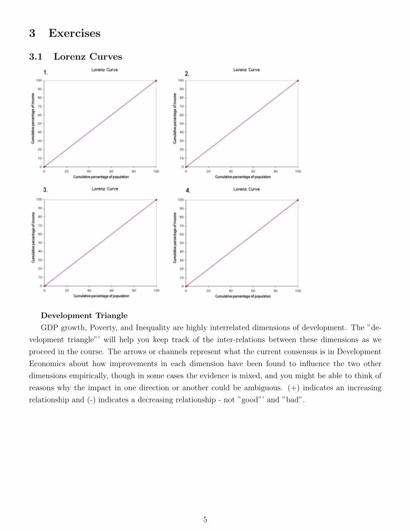
3.1 Lorenz Curves
Development Triangle
GDP growth, Poverty, and Inequality are highly interrelated dimensions of development. The ”de-
velopment triangle”’ will help you keep track of the inter-relations between these dimensions as we
proceed in the course. The arrows or channels represent what the current consensus is in Development
Economics about how improvements in each dimension have been found to influence the two other
dimensions empirically, though in some cases the evidence is mixed, and you might be able to think of
reasons why the impact in one direction or another could be ambiguous. (+) indicates an increasing
relationship and (-) indicates a decreasing relationship - not ”good”’ and ”bad”.
5

1. Growth⇒ Poverty (-): Growth generally reduces poverty, and pro-poor growth (for example, among
subsistence farmers) reduces poverty more. A cross country regression gives a elasticity of poverty
reduction with respect to growth of 2.38 (2.38% reduction in P0 with 1% growth). Note that growth
tends to be more effective in reducing poverty in the presence of a lower Gini coefficient (more equal).
2. Poverty ⇒ Growth (-): Poverty is thought to reduce growth, as poor households lack assets and/or
capital that would enable them to contribute to growth.
3. Growth⇒ Inequality (0/+): Overall, empirically we observe Kuznet’s “inverted-U” where very poor
and very rich countries tend to have lower inequality than middle-income coutnries, but there is no
clear overall causal relationship from growth to inequality (several papers have tried to establish causal
relations in one direction or another, but Banerjee and Duflo have shown problems with this whole
body of work), and the average elasticity of inquality with respect to growth is approximately zero in
cross-country regressions. In a few cases like China and Vietnam, however, rapid early growth is seen
to increase inequality, as a small portion of the population is able to take part in growth opportunities.
4. Inequality ⇒ Growth (?): This relationship is ambiguous, since there are several ways in which
inequality can influence growth, but the aggregate impact is thought to be probably (but not certainly)
negative. (See more below.)
5. Inequality ⇒ Poverty (+): In most cases, a reduction in inequality necessarily reduces poverty.
Inequality also slows the rate at which growth reduces poverty
6