section height determination methods of the isotopographic

CORRESPONDENCE Guldana D. Syzdykova [email protected]

© 2016 Syzdykova and Kurmankozhaev. Open Access terms of the Creative Commons Attribution 4.0 International License (http://creativecommons.org/licenses/by/4.0/) apply. The license permits unrestricted use, distribution, and reproduction in any medium, on the condition that users give exact credit to the original author(s) and the source, provide a link to the Creative Commons license, and indicate if they made any changes.

Introduction

Topographic and cartographic studies have begun effectively using

isogeometric analysis methods in the form of cartographic and spatial contour

lines, which have theoretical and practical advantages compared to one-

Section Height Determination Methods of the Isotopographic Surface in a Complex Terrain Relief

Guldana D. Syzdykovaa and Azimhan K. Kurmankozhaeva

aKazakh National Technical University named after K.I. Satpaev, Almaty, KAZAKHSTAN

ABSTRACT A new method for determining the vertical interval of isotopographic surfaces on rugged

terrain was developed. The method is based on the concept of determining the

differentiated size of the vertical interval using spatial-statistical properties inherent in

the modal characteristic, the degree of variability of apical heights and the chosen map

scale. It was found that the morphometric characteristics of the terrain are highly

informative, can serve as geoindicators, and have applied value; their calculation formulas

were provided. An analytical assessment of the determination of differentiated sizes of the

vertical interval was made. Its initial parameters are as follows: modal height, scale and

variability of apical heights. The vertical intervals are differentiated by dividing the

morphometric field of the terrain into two parts, the height in the contours whereof is

lower (hi < hmo) and higher (hi > hmo) than the modal height, respectively; the reasoning

behind the analytical assessment of the calculation of apical height variability and vertical

intervals, which takes into account the peculiarities of terrain formation, was given; the

main contour is drawn through the modal value of apical heights and then drawn through

other contour systems based on the calculated vertical interval values, differentiated by

the divided parts of the morphometric field.

KEYWORDS ARTICLE HISTORY Geodesy, vertical interval of the terrain,

isotopographic surface, morphometric fields, isogeometric analysis

Received 10 March 2016 Revised 20 April 2016

Accepted 28 April 2016

INTERNATIONAL JOURNAL OF ENVIRONMENTAL & SCIENCE EDUCATION

2016, VOL. 11, NO. 12, 5221-5236

OPEN ACCESS

5222 G. D. SYZDYKOVA AND A. K. KURMANKOZHAEV

dimensional analytical assessments (Blogov & Belopasov, 1974; Tomlin, 2013;

Manual of Surveying Instructions, 2009).

It is pertinent to point out that a contour line model (map, chart, etc.)

reflects the surface more effectively and to a greater extent, compared to a series

of inter-object lines, and gives ground for more hypotheses than a simple

numerical assessment of the match between the mathematical surface and its

real prototype (Triebel, Pfaff & Burgard, 2006). The depiction of the surface

terrain using contour lines is a mathematically reasonable technique that

graphically reflects the main forms of terrain and highlights their typical

morphometric peculiarities (Chung & Fabbri, 1999). The latter is achieved

primarily by choosing the optimal vertical interval, and drawing additional

contours and conditional figures (Song et al., 2008).

The effectiveness of different quantitative and qualitative maps, charts, and

other geometric models affects the reliability and quality of the results of

structural and geometric modeling of the spatial arrangement of mineral

resource signs and directly affect the assessment of mineral resource deposits

(Vallée & Sinclair, 1998). The international practice of assessing the resource

potential of minerals is based on the quality and reliability of mapping (CIM

Standards on Mineral Resources and Reserves – Definitions and Guidelines,

2000; Standards of Disclosure for Mineral Projects, 2000; Exploration Best

Practice Guidelines, 2000). With that, the main modeling parameter is the

vertical interval, i.e. the variation between the integral-valued marks of two

neighboring points of a graded projected line.

The vertical interval affects the quality, level of detail, clearness, cost, and

reliability of topographic maps and isogeometric charts. Moreover, it is an

important parameter in static geomodeling (Singer & Menzie, 2010).

Literature Review

In accordance with the current Manuals and Guidelines for topographic

surveys in CIS states, the drawing of standard vertical intervals of the terrain

mostly uses the classic formula that is derived from the basic morphometric

parameters of the terrain (Manual for Topographic Surveys at a Scale of 1:5000,

1:2000, 1:1000, 1:500, 1985; Fundamental Principles for Drawing and Updating

Topographic Maps at a scale of 1:10000, 1:25000, 1:50000, 1:100000, 1:200000,

1:500000, 1:1000000, 2005):

ℎ = 𝑎𝑡𝑔𝛽 (1)

where α is the distance between contour lines on the map (horizontal

equivalent); β is the slope of the terrain.

Equation (1) is used to determine the values of vertical intervals on

topographic maps, depending on the nature of the terrain, and to divide it into

plain terrain with a slope of β=0-2°, hilly terrain with a slope of β=2-4°, rugged

terrain with a slope of β=4-6°; mountainous or piedmont with a slope of β>6°.

The classic equation (1) is also used in its modified form when drawing

topographic maps and charts (Vilesov, 1973):

{ℎ =

𝑆

𝐾1000𝑐𝑡𝑔𝛽

ℎ =𝑆

1000𝛼𝑡𝑔𝛽

(2)

INTERNATIONAL JOURNAL OF ENVIRONMENTAL & SCIENCE EDUCATION 5223

where S is the scale of the chart; K is the number of contour lines on the

map, drawn on a section of a straight 1 mm line; α is the horizontal equivalent.

Table 1 shows the normal contour intervals (a=0.2 mm; k=1) for topographic

maps with a scale of 1:5000 – 1:100000, as well as the data on the vertical

interval provided by the Chief Directorate of Geodesy and Cartography (Manual

for Topographic Surveys at a scale of 1:5000, 1:2000, 1:1000, 1:500, 1985).

Table 1. Established sizes of the vertical interval Map scale Vertical interval, m 45%

1:5000 1 0.5-0.5 0.25-10.0

1:10000 2 2.5-2.5 0.25-10.0

1:25000 5 2.5-5.0-10.0 1.0-10.0

1:50000 10 100.0-20.0 10.0-20.0

1:100000 20 20.0-40.0 10.0-40.0

The second to last column shows the vertical interval on topographic maps

calculated at 𝓿=45°, while the last column – mostly on special maps. The data

show that the vertical interval values may be used to determine the vertical

interval on topographic maps, but cannot be used on special maps, since they are

used in engineering estimations. It is customary first to choose the vertical

interval that guarantees the accuracy of engineering estimations and then to set

the survey scale based on that.

Studies show that in the geometrization of quantitative indexes of deposits,

this classic equation is also used as a basic assessment of the contour interval in

the following form (Triebel, Pfaff & Burgard, 2006; Vilesov, 1973):

ℎ = 𝑖 ∙ ℓ (𝑖 =ℎ

ℓ), (3)

where i is the slope; ℓ is the horizontal equivalent.

It is worth noting that these classic equations take into account the

functional relation between the vertical interval and the slope and distance

between characteristic points (horizontal equivalent) of the terrain; thus, it

serves as a basis for assessing the vertical interval (Song et al., 2008). These

equations were obtained based on an analogue of a right triangle. However, such

straight lines are nonexistent on the real Earth’s surface, which means that

these equations cannot convey the actual morphometrics of the terrain. This fact

becomes obvious, considering the dynamic of changes in the slope and

elementary forms of terrain surface, which mostly determine the vertical

interval (Viduyev & Polischuk, 1973).

Scholars argue that unlike CIS states, which mostly use one vertical

interval, most countries set at least two vertical intervals for topographic maps

of the same scale (Blogov & Belopasov, 1974; Chung & Fabbri, 1999). However,

this does not imply that the optimal value of the vertical interval is achieved

simply by differentiating it. The determination of the vertical interval of the

terrain remains problematic due to the variety, different importance, and

number of factors that affects its accuracy. The promising differentiated

approach to determining the vertical interval for the topographic base requires

thorough substantiation; the conventional technique for choosing the interval

has several flaws that often cause accumulation and increase of labor costs. This

practice generally causes mismatches between the depicted and actual surface,


misperception of the level of detail and accuracy of the isotopographic maps, and

false conclusions and accumulation of suboptimal solutions.

Aim of the Study

The purpose of the study is to elaborate a method of determining the

vertical interval of isotopographic surfaces on rugged terrain.

Research questions

What are the essential requirements for differentiated sizes of the vertical

interval?

Method

The suggested method is based on the concept of determination of the

differentiated sizes of the vertical interval using the properties of the main

informative and geoindicator characteristics of apical heights, which take into

consideration the morphometric peculiarities of the terrain. The essence of the

method lies in substantiating the effective values of the vertical interval

according to structurally differentiated sections of the morphometric field of the

terrain, which reflect various sets of actual vertical interval values in this area.

It was taken into consideration that the terrain as a random field of heights

is a hidden topographic surface, which is revealed only in certain nodes with

random values across the area. Therein, an individual structural parameter may

be more hidden, which is caused by the “consistent” formation of the attribute’s

distribution structure; thus, it may serve as a natural and adequate

characteristic of the terrain attribute distribution.

The differentiation of the vertical interval is based on the concept of

geometrical division of the morphometric field of heights into separate structural

parts with different absolute values of apical heights, which are distinguished

with respect to the single modal value of the surface height. Thus, three main

optimized sizes of the vertical interval are distinguished, which are geometrized

through the modal, below-modal, and above-modal values of terrain heights. The

modal terrain height is used as a structural regulator that divides the

morphometric field into several structural sections with different absolute

values and degrees of variability of apical heights.

The area of differentiation of the vertical interval in the space of the

morphometric field of the terrain is written as follows:

{

ℎ1 ∊ 𝑄(ℎ𝑚0), 𝑆1 = ℎ𝑚𝑜

ℎ2 ∊ 𝑄(ℎ𝑖<ℎ𝑚0), 𝑆2 = ∑ ℎ2𝑖ℎ𝑚𝑜

ℎ𝑚𝑖𝑛

ℎ3 ∊ 𝑄(ℎ𝑖>ℎ𝑚0), 𝑆3 = ∑ ℎ3,𝑖ℎ𝑚𝑎𝑥

ℎ𝑚𝑜

(4)

where hmo, hmin, hmax are the modal, minimum, and maximum values of

apical heights; h1, h2, h3 are estimated effective values of the vertical interval set

on a case-by-case basis for three distinguished parts of the morphometric field of

the terrain; 𝑄(ℎ𝑚0), 𝑄(ℎ𝑖<ℎ𝑚0), 𝑄(ℎ𝑖>ℎ𝑚0) are geometric areas of distribution of

apical heights with ℎ𝑖 ≈ ℎ𝑚0, ℎ𝑖 < ℎ𝑚0, ℎ𝑖 > ℎ𝑚0; S1, S2, S3 is the sum of absolute

values of heights, respectively, for three distinguished parts of the morphometric

field of the terrain.


The nature of changes of hmo, hl, hh in the following conditions was

determined:

ℎ𝑙 − ℎ𝑚𝑜 ≈ ℎℎ − ℎ𝑚𝑜 was found in plains, including flat, lofty, billowy, and

hilly terrain;

ℎ𝑙 − ℎ𝑚𝑜 < 0, ℎℎ − ℎ𝑚𝑜 > 0 was found in hilly terrain, including large,

medium, and small hills;

ℎ𝑙 − ℎ𝑚𝑜 < 0, ℎℎ − ℎ𝑚𝑜 > 0 was found in mountainous terrain, including

high, medium, and low mountains.

In cases when the empirical distribution of terrain height is symmetrical –

ℎ𝑚𝑜 ≈ ℎ𝑎𝑣; in cases when the distribution of asymmetrical – ℎ𝑚𝑜 < ℎ𝑎𝑣.

Data, Analysis, and Results

The analytical framework of the assessment of the vertical interval in

accordance with the offered method is presented as a system of assessments in

the following form: 𝜑(ℎ0) = 𝑓(ℎ𝑚𝑜); 𝜑(ℎ𝑙) = 𝑓(ℎ𝑚𝑜𝛾𝑙 , М); 𝜑(ℎℎ) = 𝑓(ℎ𝑚𝑜𝛾ℎ, 𝑀)

{

ℎ𝑜 = ℎ𝑚𝑜

ℎ𝑙 = ℎ𝑚𝑜 − 𝛾𝑙 (М

1000)

ℎℎ = ℎ𝑚𝑜 + 𝛾ℎ (М

1000)

, (5)

where hmo is the modal value of apical heights; γl and γh are the indexes of

height variability, the values whereof are lower and higher, respectively, than

the modal height of the terrain, unit fractions; M is the denominator of the

numerical scale; hl is the sought vertical interval for areas, within the contours

of which the terrain height does not exceed the modal height (ℎ𝑙 < ℎ𝑚𝑜); ℎℎ𝑖 is

the sought vertical interval for areas, within the contours of which the terrain

height exceeds the modal height (ℎℎ > ℎ𝑚𝑜). In this case, apical heights mean

certain terrain points that are higher than the plain of the lower denudation

level.

The modal value is found with a histogram, through calculations or visually

from the observed characteristics of the distribution of terrain heights across the

area. With a sufficient amount of information, the empirical value of the mode is

found from a histogram or an ordered sample with the following equation:

𝑋𝑚𝑜 = 𝑥𝑜𝑙.𝑏. + ∆𝑥𝑅мо−𝑅мо−1

(𝑅мо−𝑅мо−1)+(𝑅мо−𝑅мо+1), (6)

where 𝑥𝑜𝑙.𝑏.is the lower boundary of the modal interval; RMO is the rate of the

modal interval; RMO-1 is the rate of the interval preceding the modal one; RMO+1 is

the rate of the interval that follows the modal one; Δx = h is the interval

variability.

The formulas of dependency between the mode and the arithmetic mean (х̅), the median (Me), and the dispersion (𝜎2) are as follows (Viduyev & Polischuk,

1973):

{𝐴 =

�̅�−𝑋𝑚𝑜

𝜎

𝑋𝑚𝑜 =𝑆(𝑆+1)

[(𝑆−1)2−𝜎𝑆|�̅�|]

(7)

where х̅ is the arithmetic mean; A is asymmetry; S is the sum of

observations; 𝜎2 is dispersion.

The Pearson correlation is a follows:


𝑋𝑚𝑜 = �̅� − 3(�̅� − 𝑀𝑒). (8)

The Kelly formula is as follows:

𝑋𝑚𝑜 = �̅� −х̅−𝑀𝑒

𝑐 , C is the constant (9)

The calculation formulas for the mode were drawn in accordance with the

theoretical distribution of probabilities (Kurmankozhaev, 2013):

with normal distribution, the mode equals the mean

𝑋𝑚𝑜 = �̅� ; (10)

with lognormal distribution

𝑋𝑚𝑜 =1

𝑛∑ 𝑙𝑔𝑋10−

𝜎2

𝑚 ; (11)

with gamma distribution

𝑋𝑚𝑜 = 𝛼 ∙ 𝛽𝜎х2

(𝛼+1) . (12)

Here 𝛼 = (Мх

𝜎х)2

− 1; 𝛽 =𝜎х2

Мх; Мх = 𝛽(𝛼 + 1), where α, β are theoretical

parameters of gamma distribution; Mx is the mean value:

with Pearson type V distribution

𝑋𝑚𝑜 =𝑉

𝑃, (13)

where V, P are the Pearson distribution parameters;

with probability-structural distribution

𝑋𝑚𝑜 = х̅ 𝑚 −𝑑2𝑡ℎ(𝑥2−𝑥0)−𝑑1𝑡ℎ(𝑥1−𝑥0)

𝑡ℎ(𝑥2−𝑥0)−𝑡ℎ(𝑥1−𝑥0) (14)

where 𝑋𝑚𝑜, 𝑥2, 𝑥1 are the modal, maximum, and minimum values of the

attribute; thx is the hyperbolic tangent; 𝑑2 = 𝑥2 − 𝑋𝑚𝑜, 𝑑1 = 𝑥1 − 𝑋𝑚𝑜.

The relation of the mode to the variability indexes (r=0.60-0.70) is also seen

from the statistical ensembles by the geomechanical attribute of durability

(N=115) of chromite minerals in the following form:

{

𝑋𝑚𝑜 = 1,482 exp(0.638𝜎) , 𝜂 = 0.61

𝑋𝑚𝑜 = 0.62 exp(0.601𝑑), 𝜂 = 0.49𝑋𝑚𝑜 = 0.81𝜎 + 0.04𝑑 − 0.78, 𝑅 = 0.76

, (15)

where 𝜎 is the standard deviation; d is the range; 𝜂, R is correlation

coefficients.

The main parameter of the model assessment that takes into account the

variability of terrain heights when differentiating the contour interval is the

structural indicator that reflects the peculiarities of the geometry of elementary

terrain surfaces through successive differences.

The new analytical assessment of the effect of variability and degree of

geometric ruggedness (curves) of the terrain surface on the vertical interval was

developed in the form of a dimensionless parameter (γ) that is expressed via

sums of successive differences of terrain heights. The geometric variability of

apical heights equals the sum of first-order successive absolute differences of

neighboring apical heights arriving at the unit of their length in the studied

morphometric field of the terrain:

𝛾𝑘 =1

𝐿∑ |∆′|𝑛𝑖=1 . (21)


For terrain surfaces with apical heights that are lower or higher than the

modal height, formula (20) acquires the following form:

{𝛾𝑙 =

1

𝐿𝑙∑ |∆′|𝑘1

𝛾ℎ =1

𝐿ℎ∑ |∆′|𝑛−𝑘𝑖=1

(22)

where γl, γh are coefficients that reflect the geometrical variability in the

parts of the terrain surface where ℎ𝑖 < ℎ𝑚𝑜 and ℎ𝑖 > ℎ𝑚𝑜, respectively; Ll, Lh are

mean parametrized lengths of the terrain surface in the parts where ℎ𝑖 <ℎ𝑚𝑜and ℎ𝑖 > ℎ𝑚𝑜, respectively; ∑ |∆′|𝑘

𝑖=1 , ∑ |∆′|𝑛−𝑘𝑖=1 is the sum of absolute first-order

successive differences of terrain heights in the parts where ℎ𝑖 < ℎ𝑚𝑜and ℎ𝑖 >ℎ𝑚𝑜, respectively; k, (n-k) are the numbers of first-order differences in the parts

the terrain where ℎ𝑖 < ℎ𝑚𝑜and ℎ𝑖 > ℎ𝑚𝑜; n is the total number of first-order

differences across the entire terrain surface.

The random location of apical heights is expressed through the mean value

of first-order successive differences as follows:

∆̅′=1

𝑛−1∑ |∆𝑖

′|𝑛𝑖=1 =

1

𝑛−1∑ |∆ℎ𝑖

′|𝑛𝑖 , (23)

where ∆𝑖′ is the absolute i value of first-order successive differences; ∆ℎ𝑖

′ is

the absolute value of first-order differences for terrain height excesses.

The mean value of first-order successive differences of apical heights, the

sizes whereof exceed the modal height (ℎ𝑖 > ℎ𝑚𝑜):

∆̅ℎ1=

1

𝑘−1∑ (𝐻𝑖

ℎ − 𝐻𝑖+1ℎ )′𝑘

𝑖=1 . (24)

The mean value of first-order successive differences of apical heights, the

sizes whereof do not exceed the modal height:

∆̅𝑙1=

1

𝑛−𝑘∑ (𝐻𝑗

𝑙 − 𝐻𝑗+1𝑙 )′𝑛−𝑘

𝑖=1 , (25)

where 𝐻𝑖ℎ, 𝐻𝑗

𝑙 are the sizes of apical heights when 𝐻𝑖ℎ > 𝐻𝑚𝑜 and 𝐻𝑗

𝑙 < 𝐻𝑚𝑜,

respectively.

The dependency between the recommended index of height variability (γi)

and terrain slope (β) results from their geometrical connection; it is expressed as

follows:

{𝛾𝐿 =

1

𝐿𝐿∑ 𝑙𝐿𝑖𝑡𝑔𝛽𝐿𝑖𝑘1

𝛾𝐻 =1

𝐿𝐻∑ 𝑙𝐻𝑖𝑡𝑔𝛽𝐻𝑖𝑛−𝑘1

, (26)

where 𝑙𝐿𝑖, 𝑙𝐻𝑖 is the distance between neighboring height values for the

lower (ℎ𝑖 < ℎ𝑚𝑜) and higher (ℎ𝑖 > ℎ𝑚𝑜) parts of the terrain surface, respectively.

The conclusion is that using the concept of modal characteristics (xmo) and

amplitude of location variability (γi) of terrain heights as the main spatial-

statistical parameters when creating a composite structure of the modal

assessment of the vertical interval is innovative and reasonable. The γ

parameters tells the presence of geometrical variability; if the amplitude

fluctuation of terrain heights is entirely random, then the value of this

coefficient 𝛾 ≈ 𝑚𝑎𝑥, i.e. shows the presence of variability, if vice versa, then 𝛾 ≈𝑚𝑖𝑛.

The results of the calculation of differentiated sizes of the vertical interval

in accordance with the developed method were obtained for comparative


analysis from three natural-experimental objects selected in different regions of

Kazakhstan. The first object is an area in the Jambyl Region, the data for which

were obtained from the results of a survey and a 1:500 chart. The terrain of the

object is plain; the variation coefficient of the elementary terrain surface height

does not exceed 40-42%; the mean height of elementary surfaces hme = 6.2 m; the

amplitude range of heights d = 28.2 m. The second object is an area in the

Glubokoye District, the data for which were obtained from the results of a

survey and a 1:1000 chart. The terrain of the object is hilly; the variation

coefficient of the elementary terrain surface height 𝑣 = 63%; the mean height of

elementary surfaces hme = 10.3 m; the amplitude range of heights d = 3.76 m.

The third object is an area in the Jualy District. The terrain of the object is

piedmont; the variation coefficient of the elementary terrain surface height is

72.5%; the mean height of elementary surfaces hme = 12.3 m; the amplitude

range of heights d = 57.2 m; the scale of the survey and topographic chart is

1:2000.

The technological order of the method execution includes three stages of

contour drawing. During the initial basic stage, the main contour is drawn on

the isosurface of the terrain. The main contour is drawn according to the modal

value of apical heights that covers at least 40-50% of all values of apical heights.

This is confirmed by the abovementioned facts, since statistical distributions of

terrain heights are described by an extremely asymmetrical radial distribution,

when about 50% of all sets of terrain height values are concentrated in the

modal value.

The high informative value, potential reliability of detection, and other

abovementioned properties of the apical height mode allow accepting the contour

that runs through its value as the main contour of the terrain isosurface.

Thus, the conventional theory that the main contours should run through

the typical points of the terrain acquires a more reasonable and substantial

meaning.

The values of apical heights that are close to the modal height should be

averaged to draw the main contour. To that end, the recommendation is to use a

mean arithmetic technique of the moving average according to the following

formula (Vilesov, 1973):

Ф = (𝑥𝑦) =1

𝑛∑ ℎ𝑖,𝑛𝑖=1 (27)

where n is the number of averaged groups of apical heights, the values

whereof are close to the modal height.

The modal value of terrain heights at the three natural-experimental

objects was found from the data of ordered samples of empirical distributions of

apical heights (Table 2). The ordered samples of height distribution in these

objects were taken with conventional techniques from the statistical ensembles

of actual values of apical heights (excesses), calculated based on topographic

surveys and charts of various scales (1:500, 1:1000, 1:2000).

The following stages of the method execution include the structural

differentiation, during which the developed analytical assessment is used to find

the sought vertical intervals in the distinguished parts of the morphometric

field, where the values of apical heights are lower (ℎ𝑖 < ℎ𝑚0) and higher (ℎ𝑖 <ℎ𝑚0) than their modal value, respectively. Contours are drawn along both parts


of the morphometric field according to the set vertical intervals with

conventional techniques.

Table 2. Collective results of the variation sets of empirical distributions of apical heights for the three natural-experimental objects № Plain-hilly terrain,

topographic survey at a scale of 1:500

Hilly terrain, topographic survey at a scale of

1:1000

Piedmont terrain, topographic survey at a

scale of 1:2000

Classes, m.

Mean, m.

Frequency, un.

fr.

Classes, m.

Mean, m.

Frequency, un.

fr.

Classes, m.

Mean, m.

Frequency, un.

fr.

1 0.1-0.6

0.3 34 0.1-0.5

0.25 17 0.1-0.5

0.25 16

2 0.6-1.2

0.9 31 0.5-1.0

0.75 13 0.5-1.0

0.75 15

3 1.2-1.8

1.5 22 1.0-1.5

1.25 10 1.0-1.5

1.25 5

4 1.8-2.4

2.1 21 1.5-2.0

1.75 11 1.5-2.0

1.75 6

5 2.4-3.0

2.7 10 2.0-2.5

2.25 5 2.0-2.5

2.25 2

6 3.0-3.6

3.3 6 2.5-3.0

2.75 2 2.5-3.0

2.75 5

7 3.6-4.2

3.9 3 3.0-3.5

3.25 3 3.0-3.5

3.25 2

8 4.2-4.8

4.5 2 3.5-40 3.75 2 3.5-4.0

3.75 1

N=129, ℎ𝑚𝑜=0,64 N=63, ℎ𝑚𝑜=0,50 N=52, ℎ𝑚𝑜=0,67

For the first object, the topographic chart is large-scale, while the terrain

category is plain; for the second object – the topographic chart is small-scale,

while the terrain category is hilly; for the third object, the topographic chart is

medium-scale, while the terrain category is medium-hilly piedmont. Therefore,

the degree of variability and fluctuation of the apical heights of elementary

terrain surfaces in these objects are different. The results of calculation of the

differentiated sizes of the vertical interval, conducted according to the modal

assessment for the three natural-experimental objects, are presented in Table 3.

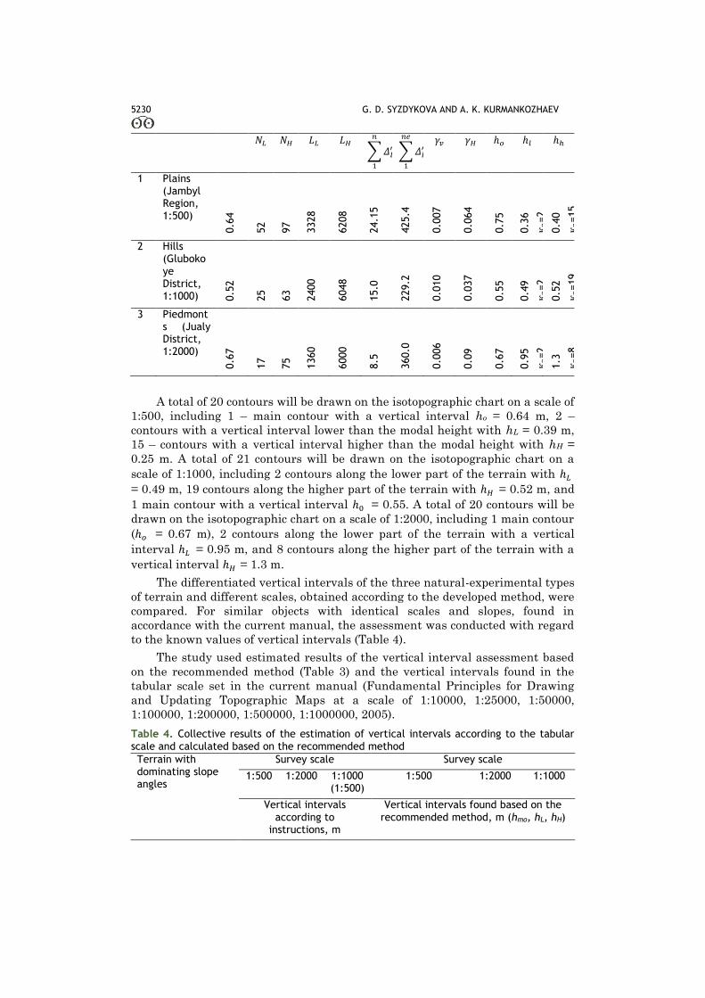
Table 3. Results of calculation of the vertical interval according to the recommended methods for areas with different scales and terrain

№ Objects and

scales

Modal value,

ℎ𝑚0, m

Number of

vertical interval

s for elemen

tary terrain surface

s

Lengths of design profiles for the terrain

surfaces, m

Sum of first-order difference

s, m.

Variability indexes of

terrain heights, un. fr.

Set vertical intervals, m.


𝑁𝐿 𝑁𝐻 𝐿𝐿 𝐿𝐻 ∑𝛥𝐿

′

𝑛

1

∑𝛥𝐻′

𝑛𝑒

1

𝛾𝑣 𝛾𝐻 ℎ𝑜 ℎ𝑙 ℎℎ

1 Plains (Jambyl Region, 1:500)

0.6

4

52

97

3328

6208

24.1

5

425.4

0.0

07

0.0

64

0.7

5

0.3

6

к2=2

0.4

0

к2=15

2 Hills (Glubokoye District, 1:1000) 0

.52

25

63

2400

6048

15.0

229.2

0.0

10

0.0

37

0.5

5

0.4

9

к2=2

0.5

2

к2=19

3 Piedmonts (Jualy District, 1:2000)

0.6

7

17

75

1360

6000

8.5

360.0

0.0

06

0.0

9

0.6

7

0.9

5

к2=2

1.3

к2=8

A total of 20 contours will be drawn on the isotopographic chart on a scale of

1:500, including 1 – main contour with a vertical interval ho = 0.64 m, 2 –

contours with a vertical interval lower than the modal height with hL = 0.39 m,

15 – contours with a vertical interval higher than the modal height with hH =

0.25 m. A total of 21 contours will be drawn on the isotopographic chart on a

scale of 1:1000, including 2 contours along the lower part of the terrain with ℎ𝐿

= 0.49 m, 19 contours along the higher part of the terrain with ℎ𝐻 = 0.52 m, and

1 main contour with a vertical interval ℎ0 = 0.55. A total of 20 contours will be

drawn on the isotopographic chart on a scale of 1:2000, including 1 main contour

(ℎ𝑜 = 0.67 m), 2 contours along the lower part of the terrain with a vertical

interval ℎ𝐿 = 0.95 m, and 8 contours along the higher part of the terrain with a

vertical interval ℎ𝐻 = 1.3 m.

The differentiated vertical intervals of the three natural-experimental types

of terrain and different scales, obtained according to the developed method, were

compared. For similar objects with identical scales and slopes, found in

accordance with the current manual, the assessment was conducted with regard

to the known values of vertical intervals (Table 4).

The study used estimated results of the vertical interval assessment based

on the recommended method (Table 3) and the vertical intervals found in the

tabular scale set in the current manual (Fundamental Principles for Drawing

and Updating Topographic Maps at a scale of 1:10000, 1:25000, 1:50000,

1:100000, 1:200000, 1:500000, 1:1000000, 2005).

Table 4. Collective results of the estimation of vertical intervals according to the tabular scale and calculated based on the recommended method Terrain with dominating slope angles

Survey scale Survey scale

1:500 1:2000 1:1000 (1:500)

1:500 1:2000 1:1000

Vertical intervals according to

instructions, m

Vertical intervals found based on the recommended method, m (hmo, hL, hH)


Plains with slope angles up to 2°

0.5 0.5 0.5 0.64; 0.40; 0.36

(1.0)

Hills with slope angles up to 4°

0.5 0.5 0.5

1.0

Rugged terrains with slope angles up to 6°

0.5 2.0 0.5 0.55; 0.49; 0.52

1.0 (1.0) 1.0

Mountainous and piedmont terrain with slope angles over 6°

1.0 2.0 1.0 0.67; 0.95; 1.3

2.0

The comparative assessment showed the following:

1) The differentiated values of vertical intervals, obtained with the

recommended method for plain (0.54 and 0.36; 0.40), rugged hilly (0.55; 0.49;

0.52), and piedmont (0.67; 0.95; 1.3) terrain do not exceed the intervals set by

the Federal Agency of Geodesy and Cartography of the Russian Federation

(Fundamental Principles for Drawing and Updating Topographic Maps at a

scale of 1:10000, 1:25000, 1:50000, 1:100000, 1:200000, 1:500000, 1:1000000,

2005) for large-scale topographic maps (0.5 ÷ 5.0 m) or the ones often used for

vertical interval maps (0.25 ÷ 10.0 m) set in accordance with manuals; however,

they differ significantly in different differentiated ranges.

2) Changes in the differentiated sizes of the vertical interval are inversely

proportional to the variability amplitude of apical heights (γL, γH), the high

values whereof correspond to small vertical intervals and vice versa.

3) The ratio of the distribution of modal height values in sets of values of

the natural-experimental objects ranged from 48 to 61%; smaller values of modal

height correspond to smaller values of apical height variability and smaller sizes

of the vertical interval, and vice versa; this directly proportional relation is

found in all three natural-experimental objects; these regularities do not

contradict the abovementioned analytical assessments of their interrelation.

4) The effect of the topographic base scale (1:500, 1:1000, 1:2000) on the

sizes of the vertical interval is proportional; it has varying significance,

depending on the variability of the terrain heights (γi).

Discussion and Conclusion

The elaboration of the theory of assessment of dependent observations is

related to successive differences and is widely used in practice. The squares of

first-order successive differences were used by Ye. I. Azbel (1976) to assess the

dispersion of a set of observations that has a regular constituent

𝜎1 = √1

2(𝑛−1)∑ (𝑥𝑖 − 𝑥𝑖+1)

2𝑛−1𝑖=1 . (16)

This formula was used by Yu.V. Linnik and A.P. Khusu (1958) to assess the

ruggedness of ground profile. In order to detect corrugations, they used the ratio

of the sum of squares of successive differences (∆′)2 to dispersion in the following

form:


𝑟 =1

2(𝑛−1)∑ (ℎ𝑖+1 − ℎ𝑖)

2/1

𝑛−1∑ (ℎ𝑖 − ℎ̅𝑐𝑝)

2𝑛𝑖=1

𝑛−1𝑖=1 . (17)

In order to assess the accuracy of the hypsometric chart, Popov B.I. used the

squares of the second-order successive differences in the following form

(Kamorny & Koscheva, 1981):

𝜎2 = √1

6(𝑛−1)∑ (𝑥𝑖 − 2𝑥𝑖+1 + 𝑥𝑖+1)

2𝑛−2𝑖=1 . (18)

Successive first- and second-order differences were used to assess the

geometry of the terrain surface as a random number in the form of a sum of

their squares (Neumyvakin, 1976). These differences are mostly used in the

following form:

𝜎𝑐𝑚 = √1

2(𝑛−1)∑ |∆𝑖

′|2𝑛

𝑖 , (19)

where ∆′ are the first-order differences of heights at i and (i+1) points; n is

the number of points (peaks).

V.M. Gudkov (1979) offers formulas expressed through sums of squares of

first-order differences to characterize the general smoothing of the (So) equation

of ore and rock contact in deposits at specific distances:

𝑆𝑜 =1

4𝑛∑ (ℎ𝑖 + ℎ𝑖+1)

2𝑛𝑖=1 . (20)

The above analytical assessments (equations 15-19) show that the first- and

second-order successive differences are suitable for assessing the variability of

attributes of a geometrical object; they reveal the nature of amplitude

fluctuations for set observation points. The absolute sum of first-order successive

differences in the terrain field assesses the sum of detected fluctuation

amplitudes and increases linearly with an increase in the amplitude. The choice

of the variability characteristic based on first-order successive differences when

differentiating vertical intervals in order to ensure the accuracy of the

assessment is reasonable.

Also can add that the vertical interval on modern topographic maps varies

significantly due to different types of terrain, the lack of standard requirements

to topographic maps, and the peculiarities of the development of cartography in

this or that country (Chentsov, 1956; Kneissl, 1957; Vermessungswesen, 1953).

In Italy, USA, and Canada, topographic maps of the same scale have at

least two vertical intervals, while in countries with different types of terrain,

such maps have 3-4 or more (Manual of Surveying Instructions: For the Survey

of the Public Lands of the United States, 2009; Manual of Instructions for the

Survey of Canada Lands, 1996). Even in small countries (Belgium, the

Netherlands), large-scale maps (1:20000, 1:25000) have two vertical intervals,

depending on the nature of the terrain in this or that area (de Leeuw, 2008). In

England, auxiliary or approximate contours are widely used for maps of the

same scale with a single accepted vertical interval; in Belgium, Denmark, and

some other countries, on 1:25000 maps and ones with a similar scale, regions

with a plain terrain have a vertical interval of 0.3-2.5.

Similar solutions are used in large-scale mapping of deposits and quarries

in India, Australia, Central and Southern African states (David, 1997; Dominy

et al., 1997). In different countries, 1:200000 (1:250000, 1:252440) maps have

different purposes, which is why the range of used vertical intervals is


considerable – from 7.6 to 305 m; 20 m and less – on topographic maps of plains

and moderately rugged regions (the Netherlands, France); 25-50 m – on maps of

countries with rugged and mountainous terrain; 60 m and more on

reconnaissance maps (underexplored regions of the USA, Canada) (Manual of

Surveying Instructions: For the Survey of the Public Lands of the United States,

2009; Manual of Instructions for the Survey of Canada Lands, 1996). The

techniques for determining the vertical interval used in Germany are somewhat

different – they use the classic equation of the geometric relation between

triangle sides to determine the normal interval (Chentsov, 1956).

To sum up, the newly developed method for determining the vertical

interval enables differentiating its sizes by discretely distinguished land plots,

which in turn provides for accurate and optimal parameters of topographic and

cartographic maps and charts.

The method contains analytical assessments of the determination of

differentiated sizes of the vertical interval, the structural initial parameters of

which are the main natural spatial-statistical characteristics of the

morphometric field of the Earth’s surface.

The concept of using the modal characteristic and amplitude variability of

terrain height location as the main spatial-statistical parameters is innovative

and applicable to the determination of the vertical interval. The main statistical-

geometric characteristic of the morphometric field is the modal height of the

terrain; it has high informative value (48-60%), unbiasedness during

assessment, real quantitative reliability, and special geometrical-statistical

properties that form the typical nonhomogeneous parts of the morphometric

field of the terrain. The spatial characteristics of the terrain morphometrics are

geometric elements (prolongation length, absolute sizes, amplitude variability,

and difference range) of the apical heights, which are structural components of

the developed analytical assessment of the height variability determination.

These structural components provide for an accurate and rational differentiation

of the vertical interval. This analytical assessment of the recommended method

that is part of the model structure reflects the degree of amplitude variability of

typical natural heights, depressions (ravines, etc.) and plains, with regard to the

selected scale and spatial length of location and changes in the values of terrain

heights.

The accuracy of isotopographic maps and charts, mathematical and

isogeometric charts, and reliability of their results when used according to the

developed method may be achieved by using differentiated sizes of vertical

intervals by drawing a contour system in the form of a single main contour along

the modal height across the parts of the morphometric field, the apical heights

whereof are lower and higher than the modal height; the most acceptable

accuracy characteristics of the reliability of the sought vertical interval that are

used in many studies are the mean squared error, random errors, interpolation

error when drawing contours, and the terrain generalization error.

Thus, the differentiated sizes of the vertical interval should meet the

following requirements:

- the vertical interval should be greater than the minimum horizontal

interval;


- the accuracy of estimation of the volume of earthwork and other

development and research works should not exceed the accuracy when using

accepted vertical intervals;

- the vertical interval should not exceed the error of determination of the

point marks on the depicted topographic function;

- the distance between the contours should ensure proper visualization and

legibility of the chart;

- the vertical interval of the topographic functions should comply with the

accuracy of the initial data and set boundaries;

- the selection of the toposurface section should be based on the

correspondence between the degree of certainty of the function and the accuracy

of the image;

- it is not necessary to use only a single calculation formula to assess the

vertical interval.

The comparative assessment of the recommended method was conducted by

calculating the differentiated sizes of the vertical interval and accuracy of its

determination in three natural-experimental areas of different scales and

terrain type. The results confirmed:

- the accuracy of estimated sizes of the vertical interval, differentiated in

accordance with the recommended method for isotopographic charts with scales

1:500, 1:1000, and 1:2000, and their comparability to the sizes of the vertical

interval found in the manuals and experience of cartographic works;

- the ability to increase the level of accuracy, detail, visualization, and

convenience of isotopographic maps and charts when using differentiated sizes

of the vertical interval determined in accordance with the recommended method.

It is worth noting that the creation of a rational analytical framework for

assessing the main morphometric parameters of the terrain not only increases

the effectiveness of topographic and cartographic products, but also is required

in a number of engineering fields that use information about terrain: in the

construction of roads, canals, telecommunication lines, in the design of aircraft

control systems, and other fields of engineering. Increasing the reliability of

toposurface mapping improves the quality of geomodeling, which in turn

improves the quality of assessment of mineral deposit resources.

Implications and Recommendations

The practical value is that the basic formulas for calculating the vertical

interval of the terrain and assessing the line that reflects the dependency of the

vertical interval on the slope and horizontal equivalent were suggested. The

further work on the research involves the examination of the proposed method

on several projects in order to reveal its advantages and disadvantages.

Disclosure statement

No potential conflict of interest was reported by the authors.

Notes on contributors

Guldana D. Syzdykova holds a PhD of Department of Mine Survey and Geodesy,

Kazakh National Technical University named after K.I. Satpaev, Almaty, Kazakhstan.


Azimhan K. Kurmankozhaev holds a Doctor of Science, Professor of Department

of Mine Survey and Geodesy, Kazakh National Technical University named after K.I.

Satpaev, Almaty, Kazakhstan.

References

Azbel, Ye. I. (1976). The Peculiarities of Studying the Statistical Structure of Variability of Ore

Quality in Deposits. Mine Survey and Geodesy, 3, 95-107.

Blogov, I. F. & Belopasov, A. A. (1974). On Topographic Survey Scales for Design and Construction.

Problems of Engineering Geodesy in Construction, 3, 17-20.

Chentsov, V. N. (1956). Vertical intervals on foreign topographic maps. Geodesy and Cartography, 3,

59-63.

Chung, C. J. & Fabbri, A. G. (1999). Probabilistic Prediction Models for Landslide Hazard Mapping.

Photogrammetric Engineering and Remote Sensing, 65(12), 1389-1399.

CIM Standards on Mineral Resources and Reserves – Definitions and Guidelines. (2000). Prepared

by the CIM Standing Committee on Reserve Definitions, October. CIM Bulletin, 93(1044), 53-

61

David, M. (1997). Geostatistical Ore Reserve Estimation. Amsterdam: Elsevier Scientific Publishing,

364 p.

de Leeuw, E. D. (2008). International Handbook of Survey Methodology. New York: Taylor & Francis,

558 p.

Dominy, S. C., Annels, A. E., Camm, G. S., Wheeler, P. & Barr, S. P. (1997). Geology in the Resource

and Reserve Estimation of Narrow Vein Deposits. Exploration and Mining Geology, 6, 317–

333.

Exploration Best Practice Guidelines. (2000). Prepared by the CIM Standing Committee on Reserve

Definitions. CIM Bulletin, 93(1044), 53-61.

Fundamental Principles for Drawing and Updating Topographic Maps at a scale of 1:10000, 1:25000,

1:50000, 1:100000, 1:200000, 1:500000, 1:1000000. (2005). GCIRR-02-006-05 Agency for Land

Resource Management of the Republic of Kazakhstan. Astana, Kazakshtan: Geodesic,

Cartographic Instructions, Regulations and Rules, 46 p.

Gudkov, V. M. (1979). Study of Variability and Distribution of the Main Attributes of Minerals: PhD

Abstract. Moscow, 32 p.

Kamorny, V. M. & Koscheva, A. I. (1981). Determining the Parameters and Assessing the Accuracy

and Location of Contours when Conducting a Topographic Survey of Continental Shelves.

Works of the Central Research Institute of Geodesy, Aerial Surveying and Cartography, 277, 22-

28.

Kneissl, J. E. (1957). Handbuch der Vermessungskunde. Wichmann Verlag, Heidelberg, 3, 53-60.

Kurmankozhaev, A. (2013). Theory of Regulation of Stabilization of Quality of ore Products During

Production. Asia-Pacific Congress for Computational Mechanics (APCOM 2013). Singapore,

December.

Liisclmer, H. (1953). Zeitschrift rur Vermessungswesen. Herausgeber und Verleger, 12(1903), 143-

154.

Linnik, Yu. V. & Khusu, A. P. (1958). Some Considerations Regarding Statistical Analysis of the

Surfaces of Ground Profile. Interchangeability and Measurement Equipment in Machine

Building. M.: Machine Building, 65-69.

Manual for Topographic Surveys at a scale of 1:5000, 1:2000, 1:1000, 1:500. (1985). Moscow: Nedra,

160 p.

Manual of Instructions for the Survey of Canada Lands. (1996). Natural Resources Canada

Geomatics Canada, 3(1), 445 p.

National Instrument 43-101 – Standards of Disclosure for Mineral Projects. (2000). Ontario

Securities Commission Bulletin 7815, 134-142.

Neumyvakin, Yu. K. (1976). Substantiation of the Accuracy of Topographic Surveys for Design.

Moscow: Nedra, 159 p.

Singer, D. A. & Menzie, W. D. (2010). Quantitative Mineral Resource Assessments. Oxford: Oxford

University Press, 219 p.


Song, J., Rubert, P., Zheng, A., & Vorburger, T. V. (2008). Topography Measurements for

Determining the Decay Factors in Surface Replication. Measurement Science and Technology,

19(8), 084005.

Tomlin, C. D. (2013). GIS and Cartographic Modeling, London: Esri Press, 324 p.

Triebel, R., Pfaff, P. & Burgard, W. (2006). Multi-level Surface Maps for Outdoor Terrain Mapping

and Loop Closing. In 2006 IEEE/RSJ International Conference on Intelligent Robots and

Systems, 2276-2282.

U.S. Department of the Interior. (2009). Manual of Surveying Instructions: For the Survey of the

Public Lands of the United States. Bureau of Land Management. Denver, CO: Government

Printing Office, 175 p.

Vallée, M. & Sinclair, A. J. (1998). Quality Assurance, Continuous Quality Improvement and

Standards in Mineral Resource Estimation. Exploration and Mining Geology, 7, 11-22.

Viduyev, N. G. & Polischuk, Yu. V. (1973). Vertical Interval and Topographic Map Scale.

Engineering Geodesy, 14, 131-137.

Vilesov, G. I. (1973). Deposit Geometrizing Techniques. Moscow: Nedra, 184 p.

section height determination methods of the isotopographic

Documents