sectoral vs. aggregate shocks: a structural factor
TRANSCRIPT
Sectoral vs. Aggregate Shocks: A Structural FactorAnalysis of Industrial Production
Andrew Foerster,Duke University
Pierre-Daniel Sarte,Federal Reserve Bank of Richmond
Mark W. Watson,Princeton University
March 2011
A. Foerster, P.-D. Sarte and M. W. Watson ()Sectoral vs. Aggregate Shocks March 2011 1 / 51

Observations and Motivating Questions
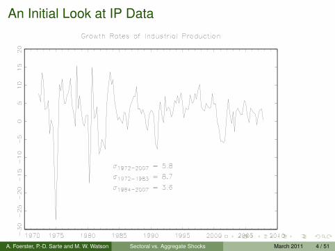
Month-to-month and quarter-to-quarter variations in IndustrialProduction (IP) are large
I std. dev. of monthly growth rates is 8 percentI std. dev. of quarterly growth rates is 6 percentI noticeably large fall in the volatility of IP after 1984
IP index is constructed as a weighted average of productionindices across a large number of sectors...
... apparently, much of the variability in individual sectors does not“average out”
A. Foerster, P.-D. Sarte and M. W. Watson ()Sectoral vs. Aggregate Shocks March 2011 2 / 51

An Initial Look at IP Data
A. Foerster, P.-D. Sarte and M. W. Watson ()Sectoral vs. Aggregate Shocks March 2011 3 / 51
An Initial Look at IP Data
A. Foerster, P.-D. Sarte and M. W. Watson ()Sectoral vs. Aggregate Shocks March 2011 4 / 51

Observations and Motivating Questions
Aggregate Shocks that affect all industrial sectors
Some sectors have very large weights in the aggregate index,Gabaix (2005)
Complementarities in production amplify and propagatesector-specific shocks
I input-output (IO) linkagesI aggregate activity spilloversI local activity spillovers
A. Foerster, P.-D. Sarte and M. W. Watson ()Sectoral vs. Aggregate Shocks March 2011 5 / 51
Approaches to analyzing sources of variations in thebusiness cycle
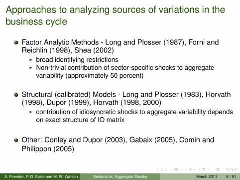
Factor Analytic Methods - Long and Plosser (1987), Forni andReichlin (1998), Shea (2002)
I broad identifying restrictionsI Non-trivial contribution of sector-specific shocks to aggregate
variability (approximately 50 percent)
Structural (calibrated) Models - Long and Plosser (1983), Horvath(1998), Dupor (1999), Horvath (1998, 2000)
I contribution of idiosyncratic shocks to aggregate variability dependson exact structure of IO matrix
Other: Conley and Dupor (2003), Gabaix (2005), Comin andPhilippon (2005)
A. Foerster, P.-D. Sarte and M. W. Watson ()Sectoral vs. Aggregate Shocks March 2011 6 / 51
Overview for this paper
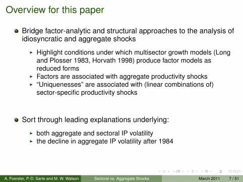
Bridge factor-analytic and structural approaches to the analysis ofidiosyncratic and aggregate shocks
I Highlight conditions under which multisector growth models (Longand Plosser 1983, Horvath 1998) produce factor models asreduced forms
I Factors are associated with aggregate productivity shocksI “Uniquenesses” are associated with (linear combinations of)
sector-specific productivity shocks
Sort through leading explanations underlying:
I both aggregate and sectoral IP volatilityI the decline in aggregate IP volatility after 1984
A. Foerster, P.-D. Sarte and M. W. Watson ()Sectoral vs. Aggregate Shocks March 2011 7 / 51
Overview for this paper
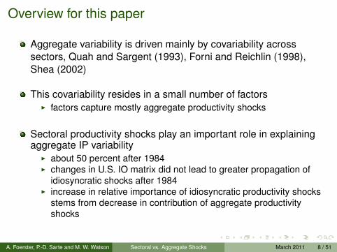
Aggregate variability is driven mainly by covariability acrosssectors, Quah and Sargent (1993), Forni and Reichlin (1998),Shea (2002)
This covariability resides in a small number of factorsI factors capture mostly aggregate productivity shocks
Sectoral productivity shocks play an important role in explainingaggregate IP variability
I about 50 percent after 1984I changes in U.S. IO matrix did not lead to greater propagation of
idiosyncratic shocks after 1984I increase in relative importance of idiosyncratic productivity shocks
stems from decrease in contribution of aggregate productivityshocks
A. Foerster, P.-D. Sarte and M. W. Watson ()Sectoral vs. Aggregate Shocks March 2011 8 / 51
Data
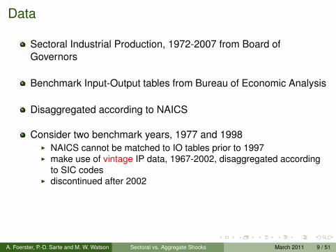
Sectoral Industrial Production, 1972-2007 from Board ofGovernors
Benchmark Input-Output tables from Bureau of Economic Analysis
Disaggregated according to NAICS
Consider two benchmark years, 1977 and 1998I NAICS cannot be matched to IO tables prior to 1997I make use of vintage IP data, 1967-2002, disaggregated according
to SIC codesI discontinued after 2002
A. Foerster, P.-D. Sarte and M. W. Watson ()Sectoral vs. Aggregate Shocks March 2011 9 / 51

Std. Dev. of Sectoral IP Growth Rates
A. Foerster, P.-D. Sarte and M. W. Watson ()Sectoral vs. Aggregate Shocks March 2011 10 / 51
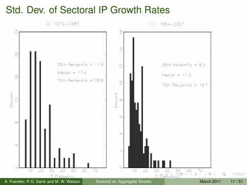
Std. Dev. of Sectoral IP Growth Rates
A. Foerster, P.-D. Sarte and M. W. Watson ()Sectoral vs. Aggregate Shocks March 2011 11 / 51

Average Pairwise Correlation of Sectoral IP Growth Rates
Monthly Growth Rates Quarterly Growth Rates72-07 72-83 84-07 72-07 72-83 84-070.08 0.13 0.05 0.19 0.27 0.11
A. Foerster, P.-D. Sarte and M. W. Watson ()Sectoral vs. Aggregate Shocks March 2011 12 / 51
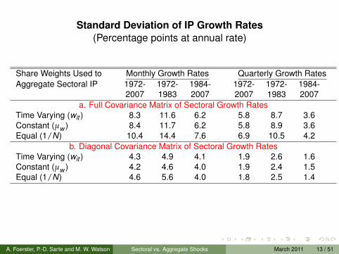
Standard Deviation of IP Growth Rates(Percentage points at annual rate)
Share Weights Used to Monthly Growth Rates Quarterly Growth RatesAggregate Sectoral IP 1972- 1972- 1984- 1972- 1972- 1984-
2007 1983 2007 2007 1983 2007a. Full Covariance Matrix of Sectoral Growth Rates
Time Varying (wit ) 8.3 11.6 6.2 5.8 8.7 3.6Constant (µw ) 8.4 11.7 6.2 5.8 8.9 3.6Equal (1/N) 10.4 14.4 7.6 6.9 10.5 4.2
b. Diagonal Covariance Matrix of Sectoral Growth RatesTime Varying (wit ) 4.3 4.9 4.1 1.9 2.6 1.6Constant (µw ) 4.2 4.6 4.0 1.9 2.4 1.5Equal (1/N) 4.6 5.6 4.0 1.8 2.5 1.4
A. Foerster, P.-D. Sarte and M. W. Watson ()Sectoral vs. Aggregate Shocks March 2011 13 / 51

Statistical Factor Analysis
Xt = ΛFt + ut
Xt is an N-dimensional vector of sectoral output growth rates, Ft isa set of r common factors, and ut is an Nx1 vector of idiosyncraticdisturbances that satisfy weak dependencePrinciple components of Xt are consistent estimators of Ft , Stockand Watson (2002)
ΣXX = ΛΣFF Λ′ + Σuu
Note: Λ and Ft are not separably identified (because ΛFt = Λ̃F̃twhere Λ̃ = ΛR and F̃t = R−1Ft for arbitrary kxk matrices R)
A. Foerster, P.-D. Sarte and M. W. Watson ()Sectoral vs. Aggregate Shocks March 2011 14 / 51

A Digression: Principle Components
The PC problem represents a way to capture the comovementacross these N categories of output changes in a convenient way
The PC problem transforms the X ’s into a new set of variablesthat...
I are pairwise uncorrelated,
I of which the first such variable has the maximum possible variance,the second the maximum possible variance among thoseuncorrelated with the first, etc...
A. Foerster, P.-D. Sarte and M. W. Watson ()Sectoral vs. Aggregate Shocks March 2011 15 / 51
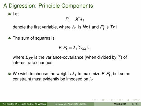
A Digression: Principle ComponentsLet
F ′1 = X ′λ1
denote the first variable, where Λ1 is Nx1 and F ′1 is Tx1
The sum of squares is
F1F ′1 = λ1′ΣXX λ1
where ΣXX is the variance-covariance (when divided by T ) ofinterest rate changes
We wish to choose the weights λ1 to maximize F1F ′1, but someconstraint must evidently be imposed on λ1
A. Foerster, P.-D. Sarte and M. W. Watson ()Sectoral vs. Aggregate Shocks March 2011 16 / 51

A Digression: Principle ComponentsThe PC problem is,
maxλ1
λ′1ΣXX λ1 + µ1(1− λ′1λ1)
The corresponding firs-order condition is,
2Σxx λ1 − 2µ1λ1 = 0.
orΣxx λ1 = µ1λ1.
Note that λ′1ΣXX λ1 = λ′1µ1λ1 = µ1. So choose the eigenvectorassociated with the largest eigenvalue of Σxx .
A. Foerster, P.-D. Sarte and M. W. Watson ()Sectoral vs. Aggregate Shocks March 2011 17 / 51

A Digression: Principle ComponentsDefine the next principle component of X as F ′2 = X ′λ2
The PC problem is
maxλ2
λ′2ΣXX λ2 + µ2(1− λ′2λ2) + φλ′2λ1.
The weights λ2 satisfy
Σxx λ2 = µ2λ2,
and, in particular, should be chosen as the eigenvector associatedwith the second largest eigenvalue of ΣXX .
A. Foerster, P.-D. Sarte and M. W. Watson ()Sectoral vs. Aggregate Shocks March 2011 18 / 51
A Digression: Principle Components
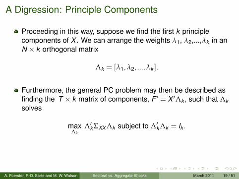
Proceeding in this way, suppose we find the first k principlecomponents of X . We can arrange the weights λ1, λ2,...,λk in anN × k orthogonal matrix
Λk = [λ1,λ2, ...,λk ].
Furthermore, the general PC problem may then be described asfinding the T × k matrix of components, F ′ = X ′Λk , such that Λksolves
maxΛk
Λ′k ΣXX Λk subject to Λ′k Λk = Ik .
A. Foerster, P.-D. Sarte and M. W. Watson ()Sectoral vs. Aggregate Shocks March 2011 19 / 51

A Digression: Principle ComponentsSolving the general PC problem is equivalent to solving
min{F1}T
t=1,...,{Fk}Tt=1,Λk
T−1T
∑t=1
(Xt −ΛkFt )′(Xt −ΛkFt ) s. t. Λ′k Λk = Ik
To see this, suppose Λk is known. Then,
Ft (Λk ) = (Λ′k Λk )−1ΛkXt
Now concentrate out Ft to get
minΛk
T−1T
∑t=1
X ′t [Ik −Λk (Λ′k Λk )Λk ]Xt s. t. Λ′k Λk = Ik
A. Foerster, P.-D. Sarte and M. W. Watson ()Sectoral vs. Aggregate Shocks March 2011 20 / 51
Statistical Factor Analysis
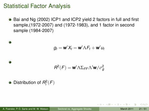
Bai and Ng (2002) ICP1 and ICP2 yield 2 factors in full and firstsample,(1972-2007) and (1972-1983), and 1 factor in secondsample (1984-2007)
gt = w′Xt = w′ΛFt + w′ut
R2(F ) = w′ΛΣFF Λ′w/σ2g
Distribution of R2i (F )
A. Foerster, P.-D. Sarte and M. W. Watson ()Sectoral vs. Aggregate Shocks March 2011 21 / 51

Statistical Factor AnalysisDecomposition of Variance from Statistical 2-Factor Model
Monthly Rates Quarterly Rates72-83 84-07 72-83 84-07
Std. Deviation of IP Growth RatesImplied by Factor Model 11.7 6.2 8.9 3.6
(with Constant Share Weights)R2(F ) 0.86 0.49 0.89 0.87
A. Foerster, P.-D. Sarte and M. W. Watson ()Sectoral vs. Aggregate Shocks March 2011 22 / 51

Factor Decomposition of Industrial Production (Monthly)
A. Foerster, P.-D. Sarte and M. W. Watson ()Sectoral vs. Aggregate Shocks March 2011 23 / 51
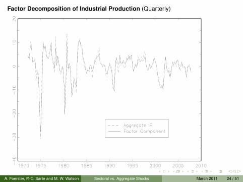
Factor Decomposition of Industrial Production (Quarterly)
A. Foerster, P.-D. Sarte and M. W. Watson ()Sectoral vs. Aggregate Shocks March 2011 24 / 51
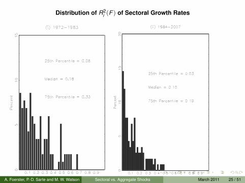
Distribution of R2i (F ) of Sectoral Growth Rates
A. Foerster, P.-D. Sarte and M. W. Watson ()Sectoral vs. Aggregate Shocks March 2011 25 / 51

Distribution of R2i (F ) of Sectoral Growth Rates
A. Foerster, P.-D. Sarte and M. W. Watson ()Sectoral vs. Aggregate Shocks March 2011 26 / 51
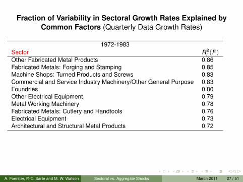
Fraction of Variability in Sectoral Growth Rates Explained byCommon Factors (Quarterly Data Growth Rates)
1972-1983Sector R2
i (F )Other Fabricated Metal Products 0.86Fabricated Metals: Forging and Stamping 0.85Machine Shops: Turned Products and Screws 0.83Commercial and Service Industry Machinery/Other General Purpose 0.83Foundries 0.80Other Electrical Equipment 0.79Metal Working Machinery 0.78Fabricated Metals: Cutlery and Handtools 0.76Electrical Equipment 0.73Architectural and Structural Metal Products 0.72
A. Foerster, P.-D. Sarte and M. W. Watson ()Sectoral vs. Aggregate Shocks March 2011 27 / 51

Fraction of Variability in Sectoral Growth Rates Explained byCommon Factors (Quarterly Data Growth Rates)
1984-2007Sector R2
i (F )Coating, Engraving, Heat Treating, and Allied Activities 0.68Plastic Products 0.67Commercial and Service Industry Machinery/Other General Purpose 0.65Fabricated Metals: Forging and Stamping 0.65Household and Institutional Furniture and Kitchen Cabinets 0.59Veneer, Plywood, and Engineered Wood Products 0.59Metal Working Machinery 0.52Foundries 0.52Millwork 0.51Other Fabricated Metal Products 0.50
A. Foerster, P.-D. Sarte and M. W. Watson ()Sectoral vs. Aggregate Shocks March 2011 28 / 51

Statistical Factor Analysis
Tracking real time movements in IP using only a subset M of theIP sectors
X̃t = sXt , where s is an M x N selection matrix
Weights, ψ, determined by projection of gt onto X̃t
ψ = (sΣXX s′)−1sΣXX w
Bulk of variation in IP explained by a small number of sectors
A. Foerster, P.-D. Sarte and M. W. Watson ()Sectoral vs. Aggregate Shocks March 2011 29 / 51

Information Content of IP Contained in Individual Sectors
Selected Sectors 1972-1983 1984-2000Ranked by R2
i (F ) Fraction of Explained IP Fraction of Explained IPTop 5 Sectors 85.0 75.4Top 10 Sectors 90.3 80.4Top 20 Sectors 97.9 86.4Top 30 Sectors 98.8 90.3
A. Foerster, P.-D. Sarte and M. W. Watson ()Sectoral vs. Aggregate Shocks March 2011 30 / 51
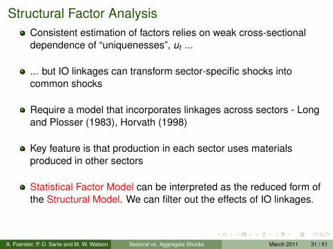
Structural Factor AnalysisConsistent estimation of factors relies on weak cross-sectionaldependence of “uniquenesses”, ut ...
... but IO linkages can transform sector-specific shocks intocommon shocks
Require a model that incorporates linkages across sectors - Longand Plosser (1983), Horvath (1998)
Key feature is that production in each sector uses materialsproduced in other sectors
Statistical Factor Model can be interpreted as the reduced form ofthe Structural Model. We can filter out the effects of IO linkages.
A. Foerster, P.-D. Sarte and M. W. Watson ()Sectoral vs. Aggregate Shocks March 2011 31 / 51
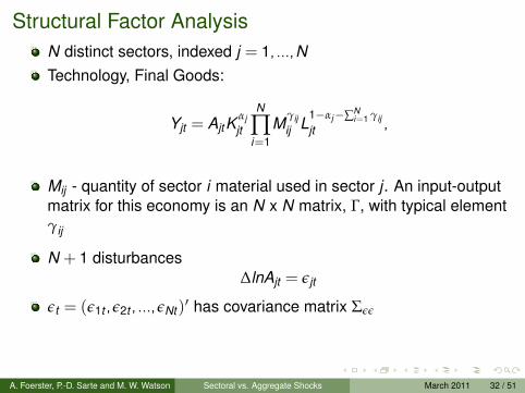
Structural Factor AnalysisN distinct sectors, indexed j = 1, ...,NTechnology, Final Goods:
Yjt = AjtKαjjt
N
∏i=1
Mγijij L
1−αj−∑Ni=1 γij
jt ,
Mij - quantity of sector i material used in sector j . An input-outputmatrix for this economy is an N x N matrix, Γ, with typical elementγij
N + 1 disturbances∆lnAjt = εjt
εt = (ε1t ,ε2t , ...,εNt )′ has covariance matrix Σεε
A. Foerster, P.-D. Sarte and M. W. Watson ()Sectoral vs. Aggregate Shocks March 2011 32 / 51

Structural Factor AnalysisTechnology: Investment Goods
Zjt =N
∏i=1
Qθijijt ,
N
∑i=1
θij = 1
Kjt+1 = Zjt + (1− δ)Kjt
Qij - quantity of sector i output used in sector j . A capital flowmatrix for this economy is an N x N matrix, Θ, with typical elementθij
A. Foerster, P.-D. Sarte and M. W. Watson ()Sectoral vs. Aggregate Shocks March 2011 33 / 51

Structural Factor Analysispreferences:
E∞
∑t=0
βtN
∑j=1
(C1−σ
jt
1− σ− ψLjt )
resource constraints:
Cjt +N
∑i=1
Mjit +N
∑i=1
Qjit = Yjt , j = 1, ...,N
Planner’s solution for sectoral output allocations,
Xt = ΦXt−1 + Πεt + Ξεt−1,
where Xt = (∆ ln(Y1t ),∆ ln(Y2t ), ..., ∆ ln(YNt ))′
Φ, Π, and Ξ are N ×N matrices that depend only on the modelparameters, αd , Γ, β, σ, ψ, and δ
A. Foerster, P.-D. Sarte and M. W. Watson ()Sectoral vs. Aggregate Shocks March 2011 34 / 51
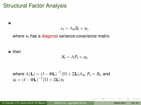
Structural Factor Analysis
εt = ΛsSt + vt ,
where vt has a diagonal variance-covariance matrix
thenXt = ΛFt + ut ,
where Λ(L) = (I −ΦL)−1(Π + ΞL)Λs, Ft = St , andut = (I −ΦL)−1(Π + ΞL)vt
A. Foerster, P.-D. Sarte and M. W. Watson ()Sectoral vs. Aggregate Shocks March 2011 35 / 51

Structural Factor Analysis
The structural model produces a an approximate factor model asa reduced form. Common factors are associated with aggregateshocks to sectoral productivity. “Uniquenesses” are linearcombinations of the sector-specific shocks.
To eliminate the propagation of sector-specifc shocks induced byIO linkages, filter the vector of sectoral output growth
εt = (Π + ΞL)−1(I −ΦL)Xt
A. Foerster, P.-D. Sarte and M. W. Watson ()Sectoral vs. Aggregate Shocks March 2011 36 / 51

Benchmark Calibration
β = 0.99, δ = 0.025, σ = 1 and ψ = 1
γij , θij , and αj obtained from IO and Capital Flow tables publishedby the BEA.
We consider two benchmark years for the IO tables, 1977 and1998
We choose two calibrations for Σεε, i) Σεε is diagonal, and ii) Σεε isrepresented by a factor model,
Σεε = ΛsΣSSΛ′s + Σvv
A. Foerster, P.-D. Sarte and M. W. Watson ()Sectoral vs. Aggregate Shocks March 2011 37 / 51

Sectoral Correlations and Volatility of IP Growth Rates Implied byStructural Model
Data Model with Model with 2 FactorsUncorrelated Shocks
Sample ρ̄ij σg ρ̄ij σg ρ̄ij σg R2(S)Period
1972-1983 0.27 8.8 0.05 5.1 0.26 9.5 0.811984-2007 0.11 3.6 0.04 3.1 0.10 4.1 0.50
A. Foerster, P.-D. Sarte and M. W. Watson ()Sectoral vs. Aggregate Shocks March 2011 38 / 51

Deconstructing the Empirical ResultsLong and Plosser (1983): Log preferences over consumption andleisure, materials delivered with a one period lag, no capital:Φ = Γ′, Π = I, Ξ = 0
Xt = Γ′Xt−1 + εt
Carvalho (2007): Same preferences, no capital:Φ = 0,Π = (I − Γ′)−1, Ξ = 0
Xt = (I − Γ′)−1εt
Horvath (1998), Dupor (1999): Log preferences overconsumption, no labor, sector-specific capital, full depreciationwithin the period Φ = (I − Γ′)−1αd , Π = (I − Γ′)−1, Ξ = 0
Xt = (I − Γ′)−1αdXt−1 + (I − Γ′)−1εt
A. Foerster, P.-D. Sarte and M. W. Watson ()Sectoral vs. Aggregate Shocks March 2011 39 / 51

Deconstructing the Empirical Results
Long and Plosser (1983):
ΣXX =∞
∑j=0
(Γ′)j ΣεεΓj
Carvalho (2007):
ΣXX = (I − Γ′)−1Σεε(I − Γ)−1
Horvath (1998), Dupor (1999):
ΣXX =∞
∑j=0
[(I − Γ′)−1αd
]j(I − Γ′)−1Σεε(I − Γ)−1
[αd (I − Γ)−1
]j
A. Foerster, P.-D. Sarte and M. W. Watson ()Sectoral vs. Aggregate Shocks March 2011 40 / 51

Deconstructing the Empirical Results
Dupor (1999) imposes 2 key restrictions on Horvath(1998)
I Γ has a unit eigenvector, so that Γl = κl , where l is the unit vectorand κ is a scalar
I all capital shares are equal, so that αd = αI, where α is a scalar
It is possible to derive simple expressions for the variance of theequally weighted aggregate growth rate,
gewt = N−1
N
∑i=1
xit
A. Foerster, P.-D. Sarte and M. W. Watson ()Sectoral vs. Aggregate Shocks March 2011 41 / 51
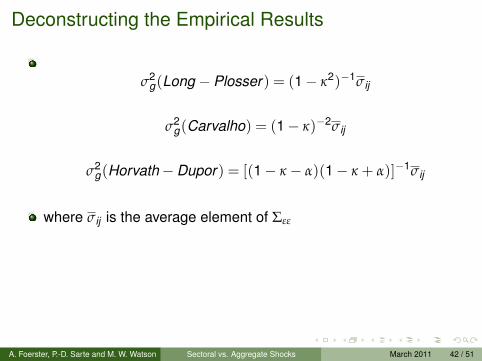
Deconstructing the Empirical Results
σ2g(Long − Plosser ) = (1− κ2)−1σij
σ2g(Carvalho) = (1− κ)−2σij
σ2g(Horvath−Dupor ) = [(1− κ − α)(1− κ + α)]−1σij
where σij is the average element of Σεε
A. Foerster, P.-D. Sarte and M. W. Watson ()Sectoral vs. Aggregate Shocks March 2011 42 / 51

Deconstructing the Empirical Results
The variance of aggregate growth is proportional to σij not only inHorvath-Dupor, but in all models
If sectoral shocks are uncorrelated, σij is their average variancedivided by N
In this case,lim
N→∞σij = 0 so that lim
N→∞σ2
g = 0
If a handful of sectors are subject to particularly large shocks,thiswill only affect aggregate variability through the average elementof Σεε
A. Foerster, P.-D. Sarte and M. W. Watson ()Sectoral vs. Aggregate Shocks March 2011 43 / 51

A. Foerster, P.-D. Sarte and M. W. Watson ()Sectoral vs. Aggregate Shocks March 2011 44 / 51

Selected Summary Statistics for Data and Various Models withUncorrelated Shocks (1972-2007 Sample Period)
ρ̄ij σg σg σgσ2
g
σ2g,Benchmark
(diag) (scaled)1 Data 0.19 5.80 1.85 5.80
2 Benchmark Model 0.04 3.87 1.88 3.82 1.00
3 Long-Plosser 0.01 2.66 2.07 2.38 0.394 Carvalho 0.04 3.15 1.64 3.56 0.875 Horvath-Dupor 0.06 3.76 1.81 3.84 1.01
6 Benchmark, Θ = I 0.02 3.86 2.43 2.94 0.597 Benchmark, δ = I 0.06 3.74 1.72 4.04 1.12
8 Long-Plosser, Γ average 0.01 1.61 1.39 2.15 0.329 Carvalho, Γ average 0.04 2.60 1.53 3.15 0.6810 Horvath-Dupor, Γ average, αd = αI 0.05 2.89 1.58 3.40 0.7911 Benchmark, Γ average, αd = αI 0.05 3.30 1.71 3.57 0.87
12 Benchmark, Σεε = σ2I 0.04 5.72 2.99 3.55 0.86
A. Foerster, P.-D. Sarte and M. W. Watson ()Sectoral vs. Aggregate Shocks March 2011 45 / 51

Selected Summary Statistics with Different Levels of SectoralAggregation
1972-1983 1984-2007ρ̄ij R2(S) ρ̄ij R2(S)
Data Model with Data Model withDiagonal Σεε Diagonal Σεε
2-Digit Level 0.38 0.09 0.76 0.22 0.07 0.53(26 Sectors)
3-Digit Level 0.29 0.05 0.85 0.13 0.05 0.53(88 Sectors)
4-Digit Level 0.27 0.05 0.81 0.11 0.04 0.50(117 Sectors)
A. Foerster, P.-D. Sarte and M. W. Watson ()Sectoral vs. Aggregate Shocks March 2011 46 / 51

Comparing Results (Model with Θ = I) Sectoral Correlations andVolatility of IP Growth Rates Implied by Structural Model
Sample Γ Data Model with Structural Model Reduced FormPeriod Uncorrelated with 2 Factors Model with 2
Shocks Factorsρ̄ij σg ρ̄ij σg R2(S) R2(S)
1972- Γ1997 0.27 8.8 0.02 3.7 0.88 0.8919831984- Γ1997 0.11 3.6 0.02 2.2 0.69 0.8720071967- Γ1977 0.21 8.5 0.03 4.0 0.83 0.8519831984- Γ1977 0.10 3.9 0.02 2.4 0.73 0.942002
A. Foerster, P.-D. Sarte and M. W. Watson ()Sectoral vs. Aggregate Shocks March 2011 47 / 51

Fraction of Variability of IP Explained by SectorSpecific Shocks
Rank Sector FractionA. 1972-1983 SIC (Θ = I)
1 Basic Steel and Mill Products 0.0642 Coal Mining 0.0343 Motor Vehicles, Trucks, and Buses 0.0084 Utilities 0.0075 Oil and Gas Extraction 0.0056 Copper Ores 0.0047 Iron and Other Ores 0.0038 Petroleum Refining and Miscellaneous 0.0039 Motor Vehicle Parts 0.004
10 Eelctronic Components 0.002
A. Foerster, P.-D. Sarte and M. W. Watson ()Sectoral vs. Aggregate Shocks March 2011 48 / 51

Fraction of Variability of IP Explained by SectorSpecific Shocks
B. 1984-2007 NAICS (Θ = I)1 Iron and Steel Products 0.0422 Electric Power Generation, Transmission and Distribution 0.0363 Semiconductors and Other electronic Components 0.0264 Oil and Gas Extraction 0.0175 Automobiles and Light Duty Motor Vehicles 0.0176 Organic Chemicles 0.0177 Aerospace Products and Parts 0.0158 Motor Vehicle Parts 0.0139 Natural Gas Distribution 0.01210 Support Activities for Mining 0.011
A. Foerster, P.-D. Sarte and M. W. Watson ()Sectoral vs. Aggregate Shocks March 2011 49 / 51
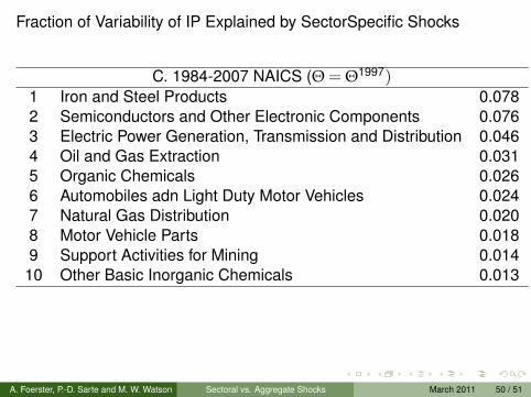
Fraction of Variability of IP Explained by SectorSpecific Shocks
C. 1984-2007 NAICS (Θ = Θ1997)1 Iron and Steel Products 0.0782 Semiconductors and Other Electronic Components 0.0763 Electric Power Generation, Transmission and Distribution 0.0464 Oil and Gas Extraction 0.0315 Organic Chemicals 0.0266 Automobiles adn Light Duty Motor Vehicles 0.0247 Natural Gas Distribution 0.0208 Motor Vehicle Parts 0.0189 Support Activities for Mining 0.01410 Other Basic Inorganic Chemicals 0.013
A. Foerster, P.-D. Sarte and M. W. Watson ()Sectoral vs. Aggregate Shocks March 2011 50 / 51

Conclusions
Neither time variation in sectoral shares of IP, nor their distribution,are important factors in explaining aggregate IP variability
Aggregate shocks largely explain variations in IP prior to 1984,and a decrease in the volatility of these shocks explain the declinein IP volatility after 1984
Relative importance of sector-specific shocks has more thandoubled over the “Great Moderation” period, from 20 percent tofully 50 percent
Changes in the structure of the input-output matrix between 1977and 1998 do not suggest a greater propagation of sectoral shocks
Analysis highlights the conditions under which multisector growthmodels first studied by Long and Plosser (1983) admit anapproximate factor representation as a reduced form
A. Foerster, P.-D. Sarte and M. W. Watson ()Sectoral vs. Aggregate Shocks March 2011 51 / 51