Contents lists available at ScienceDirect

Speech Communication

journal homepage: www.elsevier.com/locate/specom

SEDA: A tunable Q-factor wavelet-based noise reduction algorithm formulti-talker babble

Roozbeh Soleymania,b,*, Ivan W. Selesnicka, David M. Landsbergerb

a Department of Electrical and Computer Engineering, Tandon School of Engineering, New York University, 2 Metrotech Center, Brooklyn, NY 11201, USAbDepartment of Otolaryngology, New York University School of Medicine, 550 1st Avenue, STE NBV 5E5, New York, NY 10016, USA

A B S T R A C T

We introduce a new wavelet-based algorithm to enhance the quality of speech corrupted by multi-talker babblenoise. The algorithm comprises three stages: The first stage classifies short frames of the noisy speech as speech-dominated or noise-dominated. We design this classifier specifically for multi-talker babble noise. The secondstage performs preliminary de-nosing of noisy speech frames using oversampled wavelet transforms and parallelgroup thresholding. The final stage performs further denoising by attenuating residual high frequency compo-nents in the signal produced by the second stage. A significant improvement in intelligibility and quality wasobserved in evaluation tests of the algorithm with cochlear implant users.

1. Introduction

Although cochlear implants (CIs) have been highly successful atproviding speech understanding in optimal listening situations to theprofoundly deaf (e.g. Friedland et al., 2010), the performance of CIusers is severely impacted by the presence of background noise (e.g.Fetterman and Domico, 2002; Muller-Deile et al., 1995). Therefore,signal processing to remove background noise can be highly beneficialfor CI users (e.g. Dawson et al., 2011). One type of noise that has aparticularly significant effect on CI user speech understanding is “multi-talker babble” which consists of many people talking simultaneously inthe background (e.g. Sperry et al., 1997). However, multi-talker babbleis one of the most frequently encountered noises that CI users face.Hence, attenuating the speech from competing talkers is expected toprovide speech perception benefits for CI users.

Multi-talker babble is an example of a non-stationary noise. Unlikestationary signals (e.g., white noise), in a non-stationary signal, statis-tical parameters like mean, variance and autocovariance change overtime. Hence it is generally more challenging to predict or model thebehavior of a non-stationary signal over time. Although many real-timesingle-channel noise removal methods have been proposed for CI de-vices, fewer of these methods have provided benefits in non-stationarynoises such as multi-talker babble. Spectral similarities between multi-talker babble and target speech (caused by the fact that both the targetspeech and noise are comprised of speech signals) as well as the non-stationary nature of multi-talker babble make it difficult to differentiateand separate multi-talker babble from the target speech.

Yang and Fu (2005) proposed using pause detection and spectralsubtraction for noise reduction and tested the algorithm with sevenpost-lingually deafened CI users. While a significant effect of the algo-rithm was detected with speech-shaped noise, no significant effect ofthe algorithm was detected with 6 talker babble. Another noise re-duction method for CI users is to reduce the gain of the envelope ofnoise-dominated frequency channels (Bentler and Chiou, 2006). Thismethod has been commercially implemented (e.g. ClearVoice) butHolden et al. (2013) was unable to detect a significant benefit usingClearVoice with multi-talker babble.

Mauger et al. (2012) introduced an optimized noise reductionmethod by increasing the temporal smoothing of the signal to noiseratio estimate and using a more aggressive gain function. This methodwas tested in real-time on 12 CI users and significant improvement wasfound in 4 and 20 talker babble.

Goehring et al. (2016) used auditory features extracted from thenoisy speech and a neural network classifier to find and retain thefrequency channels which have higher signal to noise ratio and at-tenuate the channels with lower signal to noise ratio. Two versions ofthe algorithm (i.e., speaker-dependent and speaker-independent) weretested on 14 cochlear implant users for three different noise types in-cluding 20 talker babble. Significant improvement was achieved inmulti-talker babble specifically with the speaker-dependent algorithm.However, no significant improvement was observed in multi-talkerbabble with the speaker-independent algorithm (see Table 1).

Sigmoidal-shaped compression functions have been shown to beeffective for speech understanding against a background of multi-talker

https://doi.org/10.1016/j.specom.2017.11.004Received 24 April 2017; Received in revised form 16 October 2017; Accepted 8 November 2017

⁎ Corresponding author.E-mail address: rs4462@nyu.edu (R. Soleymani).

Speech Communication 96 (2018) 102–115

Available online 09 November 20170167-6393/ © 2017 Elsevier B.V. All rights reserved.

T

babble with 20 background talkers (Hu et al., 2007; Kasturi and Loizou,2007) by attenuating channels with a low signal-to-noise ratio (SNR).However, the perceptual and statistical properties of multi-talkerbabble depend on the number of talkers (Krishnamurthy andHansen, 2009). The more talkers present in a background noise, themore the properties of the noise resemble stationary noise. The per-formance of the sigmoidal-shaped compression functions for multi-talker babble with smaller number of talkers is not clear.

Toledo et al. (2003) observed speech intelligibility improvement formulti-talker babble in four cochlear implant users. Their method isbased on envelope subtraction and estimates the noise envelope using aminimum tracking technique (See Table 1).

Wavelet-based denoising algorithms have also been introduced forcochlear implant devices. Ye et al. (2013) proposed shrinkage andthresholding in conjunction with a critically-sampled dual-tree complexwavelet transform. While significant improvement was observed inspeech-weighted noise, no significant benefit was observed for multi-talker babble. This is expected, because the algorithm was designed forand trained with speech weighted noise.

Many other single-channel denoising methods have been proposedfor cochlear implant devices (e.g. Loizou et al., 2005; Healy et al., 2013,and Chung et al., 2004). However, only a subset of these single-channeldenoising methods have been evaluated with multi-talker babble noise.For those algorithms, which have been evaluated with multi-talkerbabble, the testing conditions, sentence corpuses, languages and typesof babble noise vary across studies and therefore it is difficult to com-pare the effectiveness across algorithms. It is worth noting that mostalgorithms provided statistically significant improvements only for highSNRs. For reference, the results and testing conditions for some of thesedenoising algorithms are summarized in Table 1.

In this paper, we propose and evaluate a front-end babble noisereduction algorithm. Although the algorithm is not necessarily specificfor CI users, we evaluate performance of the algorithm with CI usersbecause they stand to benefit greatly from noise reduction for positiveSNRs where we expect the algorithm to perform best.

2. Algorithm

The babble noise reduction problem can be summarized as

∑= +=

Y S Si

n

i1 (1)

where Y is the noisy signal, S is the target speech and S1 to Sn areindividual background talkers which collectively form the multi-talkerbabble. For developing the algorithm, we made the following assump-tions:

1. Target speech and background babble both consist of human speech.This makes it difficult to distinguish the target speech from thebackground babble.

2. Babble, which comprises of multiple independent speech signals, is

likely to have a different level of information disorder or uncertaintythan a single talker. Features such as entropy, which measure theunpredictability of information content of a signal might be helpfulto differentiate target speech from the babble.

3. Target speech is louder (i.e., has greater amplitude variance) thaneach individual background speaker, i.e.:

> ∀ ≤ ≤σ σ i n1 .S S2 2

i (2)

Consequently, in a noisy speech frame, samples originating from thetarget speech are more likely to have a larger amplitude than sam-ples originating from the babble. Hence, thresholding (which can beused to separate large-amplitude samples from the small-amplitudesamples) can potentially solve the babble problem. Note that (2)does not imply that the energy of the target speech is necessarilygreater than the total energy of the multi-talker babble. In fact, it ispossible that the Signal to Noise Ratio (SNR) is negative while (2)still holds.

However, a simple temporal or spectral thresholding cannot ade-quately solve such a complex problem as separating one talker from ababble background. There are two reasons for the ineffectiveness ofsimple temporal/spectral thresholding for babble reduction: First,babble and speech are highly overlapping in time and frequency.Second, some target speech coefficients in the time or frequency do-main are inevitably smaller than the threshold level and will be atte-nuated or set to zero by the thresholding. Moreover, in practice thenoise level is unknown and this makes it difficult to estimate a suitablethreshold level. In the following sections, we propose a solution to theseproblems by designing a classifier to estimate the noise level and ap-plying adaptive group thresholding in an oversampled wavelet domainto minimize the overlapping and distortion problems.

In our proposed algorithm, SEDA (Speech Enhancement usingDynamic thresholding Approach), every incoming frame of the noisyspeech will go through the following three steps: (1) classification, (2)denoising, and (3) enhancement. The classification stage classifies theincoming noisy frames as being either speech-dominated or noise-dominated. The denoising stage performs adaptive group thresholdingin a wavelet domain to attenuate components which primarily originatefrom babble. The threshold levels in the denoising stage are adjusted inreal-time based on the results of the classification stage. Finally, in theenhancement stage, a low pass filter is applied to the noise-dominatedframes to eliminate high frequency artifacts resulting from the de-noising stage (see Fig. 1).

2.1. Classification

The proposed classifier categorizes relatively short frames of theinput signal (consisting of the combination of target speech and thebackground multi-talker babble) as being either noise-dominated orspeech-dominated based on the frame's Signal-to-Noise-Ratio (SNR). Incontrast to overall SNR which is estimated over the entire length of the

Table 1Summary of results and testing conditions for previous studies investigating denoising of multi-talker babble. Note that the improvement observed was not significant for four of the ninetests. The non-significant improvements are indicated with “(n.s.)”.

Method Babble type / Source Mean improvement Comments

Yang and Fu (2005) 6 Talker /Unknown 7.75 % (n.s.) 7 Subjects in 0, 3, 6 and 9 dB SNRsHu et al. (2007) 20 Talker / AUDITEC CD 10–25% 9 Subjects 5 dB SNR, 5 Subjects 10 dB SNRKasturi and Loizou (2007) 20 Talker / AUDITEC CD ∼ 11% 9 Subjects in 5 and 10 dB SNRsYe et al. (2013) 20 Talker / Unknown ∼ 0.39 dB SRT (n.s.) 9 Subjects, SRT testMauger et al. (2012) 4 - 20 Talker / Unknown 5–7% 12 Subjects, SNR(50%) and SNR(50%)-1dBToledo et al. (2003) Unknown / AUDITEC CD ∼ 8% (n.s.) 4 Subjects in 5 dB SNRDawson et al. (2011) Cocktail Party / Field Recording 0.87–1.09 dB SRT 13 Subjects, SRT testGoehring et al. (2016) 20 Talker / AUDITEC S.L. 0.4 dB SRT (n.s.) 14 Subjects, SRT test, speaker-independent

2 dB SRT 14 Subjects, SRT test, speaker-dependent

R. Soleymani et al. Speech Communication 96 (2018) 102–115

103

signal, the local SNR is estimated over relatively short frames of thenoisy signal. In the example illustrated in Fig. 2, the short frames are100ms in duration. This figure shows the values of the local SNR in 10seconds of noisy speech (i.e., 100 non-overlapping frames) corrupted by10 talker babble with an overall SNR of 6 dB. Frames with a positiveSNR are considered to be speech-dominated while frames with negativeSNRs are considered to be noise-dominated. However, to avoid classi-fying frames with negligible SNR difference into different classes, anarrow buffer zone is defined between −1 dB and +1 dB SNR. Frameswith SNRs within this buffer can be correctly classified as either speech-dominated or noise-dominated. A database of 2100 sentences, including720 male speaker and 720 female speaker IEEE standard sentences(IEEE Subcommittee, 1969), 260 male speaker HINT sentences(Nilsson et al., 1994) and 400 male speaker SPIN sentences(Bilger et al., 1984) was used to create babble and speech samples.

To create each babble sample, the number and gender of talkerswere randomly selected. The number of talkers varied from 5 to 10. Theframe duration was selected to be 128ms. As a result, the frame lengthvaries as a function of sampling rate.

2.1.1. Feature selectionFour features sensitive to changes of SNR in short frames of target

speech mixed with multi-talker babble noise, were selected. Forevery incoming noisy speech frame Fi, a feature vectorF = f f f f[ , , , ]i i i i i

(1) (2) (3) (4) is formed. Our selected features are as fol-lows:

Entropy fi(1): To compute this feature, we compute the entropy of

each frame using its histogram as follows:

∑ ∑= − = − ⎛⎝

⎞⎠= =

f P k log P k h kL

log h kL

( ) ( ( )) ( ) ( )i

k

N

k

N(1)

110

110

(3)

where h is the amplitude histogram of Fi, P(k) is the probability of thekth bin, N is the number of bins and L is the frame's length. Because L isa constant, to avoid extra computation we simplify (3) and calculate the

feature as: = − ∑ =f h k log h k( ) ( ( ))i kN(1)

1 10 . The value of this feature in-creases with increasing frame SNR.

Post-thresholding to pre-thresholding RMS (Root Mean Square)ratio fi

(2): The value of this RMS ratio increases with increasing frameSNR. To compute this feature, first we set a threshold level τ(Fi ):

=τ FL

F( ) 1 Ki i 1 (4)

where ‖Fi‖1 is the l1 norm of the frame Fi. Then we find Fith by hard

thresholding Fi with threshold level τ(Fi). Finally, we calculate the ratioof the RMS values of Fi

th and Fi.

=frms Frms F

( )( )i

ith

i

(2)

(5)

Envelope Variance fi(3): The variance of the frame's envelope in-

creases with the frame's SNR. To obtain this feature, we first computethe frame's envelope ei as follows:

∑= +=−

e nL

F k nh w k( ) 1 ( ) ( )iw

k Li

2w

Lw2

(6)

where, Lw is the window length, w is the window and h is the hop size.Here we use non-overlapping rectangular windows with h= Lw. Thenwe find the normalized envelope ei :

=e n e ne

( ) ( )max( )i

i

i (7)

and finally, we calculate the envelope variance:

∑= = −=

fN

e n μvar(e ) 1 ( ( ) )iw

N

i i(3)

in 1

2w

(8)

where, Nw is the total number of windows in a frame and= ∑ =μ e n( )i N

Ni

1n 1w

w .

Envelope Mean-Crossing fi(4): The envelope mean-crossing de-

creases with increasing frame's SNR. To extract this feature first wecompute the envelope ei using (6). Then we calculate the envelopemean-crossing as follows:

∑= − − − −=

( ) ( )fN

μ μ12

sign e (k) sign e (k 1)iw

N(4)

k 2i e i e

w

i i(9)

where: ei and μei are the normalized envelope and its mean respectivelyand sign(x) is defined as:

=⎧⎨⎩

>− <

=

xxx

sign(x)1, 0

1, 00, 0

2.1.2. Feature optimizationFor each of the previously discussed features, the quality can be

estimated using a Fischer score (Tang and Liu, 2014; Gu et al.,2012;Duda, 2001):

12

3

Fig. 1. SEDA overall block diagram.

0 20 40 60 80 100

-20

-10

0

10

20

SN

R (d

B)

Frame NumberFig. 2. Local SNR for noisy speech sample with overall SNR=6. Frame dura-tion= 100 ms.

R. Soleymani et al. Speech Communication 96 (2018) 102–115

104

=∑ −

∑=

=

Sn μ μ

n σ

( )jN

j j

jN

j j

12

12

c

c(10)

where Nc is the number of classes (i.e., =N 2c ), μj is the mean of thefeature in class j, μ is the overall mean of the feature, σj is the varianceof the feature in class j, and nj is the number of samples in class j. Tooptimize the quality of features, (10) was numerically maximized foreach feature and the suitable values for feature parameters were se-lected. Table 2 shows the selected values for parameters which de-termine the quality of each feature.

2.1.3. Weighted PCA (Principle component analysis)To reduce the correlation (redundancy) between the features, we

use PCA to generate a new smaller set of uncorrelated features.Assuming F is the feature matrix and NF is the total number of noisyspeech frames, we can write:F F F F= [ , . .. ]N1 2 F . First we findF 0 byremoving the mean of features as follows:

F F= − M0 (11)

whereM is the mean matrix of features. The goal is to find the trans-formation matrix T, such that:

F F= Td 0 (12)

where,F d is the de-correlated feature matrix. The covariance matrix C0

of F 0 can be obtained as follows:

F F=CN1 .T

0 0 0 (13)

Using (12) and (13) we can write (Shlens, 2003; Bishop, 2007; Bello,2016):

F F F F F F= = = ⎡⎣

⎤⎦

=CN N

T T TN

T TC T1 1 [ ][ ] 1d d d

T T T T T0 0 0 0 0

(14)

where, Cd is a diagonal rank-ordered covariance matrix of uncorrelatedfeature matrix F d. In order to diagonalize the symmetric matrix of C0

we compute the orthogonal matrix of its eigenvectors. Assuming r is therank of covariance matrix C0, the eigenvectors of C0 and their asso-ciated eigenvalues can be written as: {v1, ⋯v v, }r2 and { ⋯λ λ λ, , r1 2 }such that: =v λ vC i i i0 . Now we define: = v v vV [ . . . ]r1 2 and using(14) we have (Shlens, 2003; Bishop, 2007; Bello, 2016):

= ⇒ =C V C V T VdT T

0 (15)

The transform matrix T is a matrix whose rows are the eigenvectorsof the covariance matrix C0. Having T, we can de-correlate the originalfeature vector F0 using Eq. (12). Because we have four original features,in the case of r < 4 we select − r4 arbitrary orthonormal vectors andcomplete the V. These orthonormal vectors do not change the resultbecause they are associated with zero variance features (Shlens, 2003).To take the quality of each feature into account we give a relativeweight to each feature based on its Fischer quality score. The weightedcovariance matrix C0 will be obtained as (Yue and Tomoyasu, 2004):

F F= =⎡

⎣

⎢⎢⎢

⎤

⎦

⎥⎥⎥

CN

W W

SS

SS

1 W and

0 0 00 0 00 0 00 0 0

T T0 0 0

1

2

3

4 (16)

where, W is the weighting matrix and S1–S4 are the average Fischerscores of the four original features. After completing this stage, we havefour new de-correlated features which are ranked based on their var-iances. We selected the first two features with the highest Fischer score(see Fig. 3).

2.1.4. Training with GMMTo train the classifier, we use the two dimensional Gaussian Mixture

Model (GMM) where each class is modeled as the sum of a n Gaussiandistributions as follows: (Reynolds, 2009):

F N F

F F

∑

∑

=

= −

=

=

− − −−{ }

G μ w C w μ C

wπ C

e

( , , ) ( , )

(2 )

di

n

i d i i

i

ni

i

μ C μ

1

1

12 [ ] [ ]

dd i

Ti d i

2

1

(17)

where F d is a two-dimensional de-correlated feature matrix usingweighted PCA and wi, μi and Ci are the weight factor, mean and cov-ariance of the ith Gaussian distribution respectively. We also shouldhave ∑ == w 1i

ni1 .

The probability of a data sample k with a feature vector F d(k)belonging to a Gaussian j can be calculated as (Bishop, 2007; Bello,2016):

N F

N F=

∑ =p

w k μ C

w k μ C

( ( ) , )

( ( ) , )jk j d j j

in

i d i i1 (18)

In order to train our model, we use the iterative Expectation-Maximization (EM) algorithm (Bishop, 2007, Reynolds et al., 2000;Reynolds, 2009; Bello, 2016). In order to fit a Gaussian to each clusterwe should maximize the following logarithmic function (Bishop, 2007;Bello, 2016):

F N F∑ ∑= ⎧⎨⎩

⎫⎬⎭= =

p μ C w w k μ Clog{ ( , , )} log ( ( ) , )dk

N

i

n

i d i i1 1

F

(19)

where NF is the number of data samples (i.e., the number of audioframes).

We first initialize wi, μi, Ci and calculate pik, then update wi, μi, Ci

using the calculated values of pik (Bishop, 2007; Bello, 2016):

Table 2Selected values for feature parameters by numerically maximizing Fischer score. Valuesare selected for frame duration of 128 ms and sampling rate of 16,000 samples persecond. B is the bin width in histogram, M is the long term maximum amplitude of thenoisy signal (constant), K is the threshold coefficient in Eq. (4) and Lw is the windowlength in Eq. (6).

Feature Parameter Selected value

fi(1) �∈B 0.05Mfi(2) �∈K 3fi(3), fi(4) �∈Lw 50

−3 −2 −1 0 1 2 3 4−3

−2

−1

0

1

2

3

4

Decorrelated Feature1

Dec

orre

late

d F

eatu

re2

Speech Dominated

Noise Dominated

Fig. 3. Scatter plot of de-correlated features 1 and 2 computed over 25,000 randomlygenerated noisy speech frames corrupted with multi-talker babble with random SNR andnumber of talkers (Between 5–10). Blue dots represent the noise-dominated frames andred dots represent the speech-dominated frames. Frame duration = 128 ms, Samplingrate= 16,000 samples per second.

R. Soleymani et al. Speech Communication 96 (2018) 102–115

105

F

F F

=∑

∑=

∑

=∑ − −

∑

μp k

pω

pN

Cp k μ k μ

p

( )

( ( ) )( ( ) )

inew k i

k

k ik i

new k ik

F

inew k i

kd i

newd i

new T

k ik

d

(20)

We repeat the above stages until the convergence of (19). We cantrain our classifier with only one Gaussian for each class to avoid heavycomputation. By increasing the number of Gaussians the classifier ac-curacy will slightly increase (See Fig. 4). In the final algorithm, aclassifier with only one Gaussian for each class was trained.

2.1.5. Classification using MAP (Maximum a posteriori estimation)After the classifier is trained, we find the probability of each test

feature set F d belonging to a class X by (Duda, 2001; Bello, 2016):

Fargmax P class P class[ ( ) ( )]X d X X (21)

X ∈ { S, N} S: Speech-Dominated N: Noise-Dominated.

F N F∑==

P class w μ Cwhere ( ) ( , ).d Xi

n

i d i i1 (22)

μi, Ci and wi are also available from the GMM training process.The values of P(classN) and P(classS) change as a function of the

overall (long term) SNR and can be obtained during training by com-puting the number of each class occurrence divided by the total datasamples in training data for each overall SNR. If the overall SNRchanges very quickly (i.e., fast varying noisy condition) we can assume

= =class P class( ) ( ) 0.5N S . In most of the cases the general noise leveldoes not change quickly (i.e., slow varying overall SNR). In this situa-tion we can estimate more accurate values for P(classN) and P(classS) byroughly estimating the overall SNR. To estimate the overall SNR wesuggest a very simple classifier which classifies the long frames of thenoisy speech (i.e., four seconds long) into one of the 6 classes listed inTable 3 and choose the P(classN) accordingly.

The overall SNR classifier uses only two of the features mentionedearlier in this section (RMS ratio and envelope mean crossing) calcu-lated over the long frames of the noisy speech without de-correlatingthe features with PCA. We use GMM with a single Gaussian per class fortraining the overall SNR classifier (see Fig. 5). Note that the in-dependent accuracy of the overall SNR classifier is not a concern.However, this classifier works as a component of the SEDA classifier

and its accuracy will affect the accuracy of SEDA classifier. The SEDAclassifier's accuracy is measured in the next section. P(classN) and P(classS) should be continuously updated based on the estimated overallSNR and the frequency of overall SNR detection update depends on ourassumption of how fast the noisy environment varies. In this work weupdated P(classN) and P(classS) once every four seconds.

2.1.6. Performance evaluationThe performance of the classifier was evaluated using two-fold cross

validation (Kohavi, 1995). First, the classifier was trained with noisyspeech samples randomly created from half of the sentence database(with random number and gender of talkers). Then the resulting clas-sifier was evaluated using test samples created from the second half ofthe sentence data base. Subsequently, the following accuracy metricswere computed:

=+

=+

=++ −P C

C fR C

C fF P R

P R2

N(23)

where C, +f and −f are correct, false positive and false negative de-tection, respectively. Then we swapped the testing and training data-bases and repeated the same process and obtained new values for ac-curacy metrics. Finally, we averaged the resulting two values for eachaccuracy metric as per two-fold cross validation method (Powers 2011;Swets 1988; Bello, 2016).

Fig. 6 shows the calculated F accuracy metric for a classifier trainedwith a single Gaussian for each class. The same result was achieved bytesting the classifier with 10-talker babble extracted from the AzBiotesting material which consists of 5 male and 5 female speakers (Rolandet al., 2016).

−3 −2 −1 0 1 2 3 4−3

−2

−1

0

1

2

3

4

5

Decorrelated Feature 1

Dec

orre

late

d F

eatu

re 2

−2 0 2 4−3

−2

−1

0

1

2

3

4

5

Decorrelated Feature 1

Dec

orre

late

d F

eatu

re 2

G3

G2

G1G1

G2

G3

G1

G1

Noise Dominated

Speech DominatedSpeech Dominated

Noise Dominated

Fig. 4. GMM plots using EM method with only one Gaussian per class (left) and three Gaussians per class (right). computed over 10 h (281,250 frames) of randomly generated noisyspeech frames corrupted with multi-talker babble with random SNR and number of talkers (between 5–10). Frame duration=128 ms, Sampling rate= 16,000 samples per second.

Table 3Selected values for P(classN) for various overall SNR classes. Note that

= −class P class( ) 1 ( )S N .

Overall SNR P(classN)

SNR<−1.5 dB 0.8171−1.5 dB < SNR < 1.5 dB 0.65991.5 dB < SNR < 4.5 dB 0.49074.5 dB < SNR < 7.5 dB 0.36457.5 dB < SNR < 10.5 dB 0.2695SNR>10.5 dB 0.1941

R. Soleymani et al. Speech Communication 96 (2018) 102–115

106

To train the final SEDA classifier, we used half of the sentence database to create multi-talker babble samples. We used the other half tocreate multi-talker babble for the listening test described in Section 3.As was done for the classifier evaluation, we randomized the numberand gender of talkers to train the final classifier. IEEE standard sen-tences with male speakers were used to create the target speech for thelistening test (see Section 3). Hence for training the final SEDA classifierwe did not use IEEE sentences with male speaker as target speech.

2.2. Denoising

Sparsification using an oversampled wavelet transform is an effec-tive way to minimize the overlapping between signal and noise coef-ficients. However, sparsification is an iterative process which oftencannot be implemented in real-time algorithms due to its high com-putational requirements. Moreover, human speech cannot be efficientlysparsified in most wavelet domains unless we implement additionalmeasures (e.g., Morphological Component Analysis; MCA) (Selesnick,2010; Selesnick, 2011a). The representation of the clean speech sam-ples in an oversampled Tunable Q-factor Wavelet Transform (TQWT;Selesnick, 2011b) exhibits some degree of group sparsity which doesnot exist in babble samples. SEDA takes advantage of this property(among others) to denoise the speech samples which are corrupted bymulti-talker babble.

Note that increasing the oversampling rate of a wavelet transformwill increase number of samples and consequently the required

computation by the same factor. Hence using a conventional filter bankin which each output channel has the same sampling frequency as theinput signal has the disadvantage of increasing the computational costsin real-time applications. TQWT provides the ability to optimize theoversampling rate. A TQWT is defined by three parameters which canbe adjusted independently: Q-factor, the redundancy, and the numberof levels (Fig. 7). The Q-factor is a measure of the oscillatory behaviorof a pulse; it is defined in terms of the spectrum of the pulse as the ratioof its center frequency to its bandwidth. The redundancy is the over-sampling rate of the wavelet transform and is always greater than 1. Bychanging these parameters, we can obtain different representations ofthe signal in the wavelet domain. We use this property later in thispaper in parallel denoising technique. Another advantage of the TQWTis in its spectral properties, namely the frequency responses of its sub-bands, are consistent with the human auditory system. The distributionof the center frequencies of the sub-bands and the shape of the fre-quency responses of the TQWT resemble Mel-scale and Gammatonefilter banks that are designed to reflect the human auditory system(Fig. 7).

2.2.1. Adaptive group thresholdingWe propose an adaptive group thresholding of the TQWT domain

coefficients of the noisy speech, based on the following strategies:

1. For each sub-band i in the TQWT domain, the threshold level shouldbe just enough to remove most of the babble noise with minimum

0 100 200 300

0.1

0.2

0.3

0.4

0.5

Envelope Mean−Crossing Rate (Per Second)

Bef

ore

/ afte

r th

resh

oldi

ng r

atio

G1 (SNR<−1.5dB)

G3 (1.5 dB< SNR < 4.5dB)

G4 (4.5 dB< SNR < 7.5dB)

G6 (SNR > 10.5dB)

G2 (−1.5 dB< SNR < 1.5dB)

G5 (7.5 dB< SNR < 10.5dB)

Fig. 5. GMM plots using EM method with only one Gaussian perclass for overall SNR classifier. Computed over 50,000 longframes of randomly generated noisy speech corrupted with multi-talker babble with random SNR and number of talkers (between5–10). Long Frames Duration= 4 s, Sampling rate=16,000samples per second.

−3 0 3 6 9 12 150.8

0.85

0.9

0.95

1

SNR (dB)

Cla

ssifi

er F

Met

ric

10 Talker Babble (5 Female, 5 Male)6 Talker Babble (3 Female, 3 Male)4 Talker Babble (2 Female, 2 Male)

Fig. 6. Accuracy metric (F) of SEDA classifier measured over1 h of noisy speech corrupted with multi-talker babble foreach overall SNR and babble type using two-fold cross vali-dation method.

R. Soleymani et al. Speech Communication 96 (2018) 102–115

107

0 0.1 0.2 0.3 0.4 0.50

0.2

0.4

0.6

0.8

1

FREQUENCY RESPONSES: Q = 2.00, R = 3.00

NORMALIZED FREQUENCY (HERTZ)

0 50 100 150 200 250 300 350 400 450 500

14

13

12

11

10

9

8

7

6

5

4

3

2

1

TIME (SAMPLES)

DN

AB

BU

S

WAVELETS: SUBBANDS 1 THROUGH 14. Q = 2.00, r = 3.00

0 0.5 1 1.5 2 2.5 3 3.5 4 4.5 5

14

13

12

11

10

9

8

7

6

5

4

3

2

1

TQWT SUBBANDS OF A CLEAN SPEECH SAMPLE DURATION=5 SEC. Q = 2.00, r = 3.00, Levels = 13

TIME (SECONDS)

DN

AB

BU

S

Fig. 7. Frequency response (top left) sub-band wavelets (bottom left) and sub-band coefficients (right) of a TQWT with = = =Q r J2, 3, 13.

S N S N N S N N S. . . . .

Previous Signal Blocks Current Signal Block. . .

. . .

. . .

. . .

. . .

N

. . .

. . .

. . .

( )

(25)

N: Noise Dominated. S: Speech Dominated.

( ) ( ) ( ) ( ) ( )

( )

( )

( ) ( )

( )

( )

( )

( )

( )

( )

( )

( )

( )

( )

( )

( )

( )

( )

(26)

Fig. 8. Block diagram of average noise level updating process.

R. Soleymani et al. Speech Communication 96 (2018) 102–115

108

distortion of the target speech. Hence for a given sub-band i we needto know the noise level in order to select the appropriate thresholdlevel. If the current noisy speech frame is speech-dominated, weestimate the noise level based on the average noise level in the samesub-band over the last few noise-dominated frames.

2. For every frame, we divide each TQWT sub-band into multipleshorter segments (i.e., coefficient-group) where each coefficient-group consists of a few coefficients (SEDA works with 16 coefficientsper coefficient-group). Hard and soft thresholding will be used al-ternatively for different coefficient-groups.For a real-valued signal x, hard and soft thresholding with thresholdlevel T are defined with HT(x) and ST(x) as follows:

= ⎧⎨⎩

≤> =

⎧⎨⎩

+ < −− ≤ ≤

− >H x x T

x x T S xx T x T

T x Tx T x T

( ) 0,, ( )

,0,

,T T

(24)

Hard thresholding will be used for coefficient-groups with small l1norm value. This will remove many small coefficients originatingfrom the noise source. Recall that target speech is louder than anyindividual background talker and has some degree of group sparsityin TQWT domain, therefore low amplitude coefficients scatteredacross the sub-band without forming a distinct group of coefficients,are more likely to originate from the babble source. A milder softthresholding (with a smaller threshold level) will be used for coef-ficient-groups with large l1 norm. This will prevent distortion whena mixture of large and small coefficients coming from target speechare concentrated in a group/cluster (see Fig. 8). Using an aggressivehard thresholding in these cases would eliminate the smaller coef-ficients and would lead to distortion.

3. General thresholding aggressiveness (level) for each frame is alsodetermined based on the result of the classification. A more ag-gressive thresholding is used for noise-dominated frames whereas aless aggressive thresholding is used for speech-dominated frames.Details are given in following sub-sections.

Updating the threshold levelAs previously mentioned, threshold levels in each sub-band depend

on the average noise level over the last few noise-dominated frames. Toupdate the noise level estimation for every incoming frame we definean array μ as follows:

∑=⎡

⎣

⎢⎢⎢

⎤

⎦

⎥⎥⎥

=

= … =

+=

+

μ

μμ

μμ

Mw

w w w w φ F

..where: 1 and

{ , , , } ( )

J

ik

ik

k k kJ

kn

k

1

2

11

M( )

1

( )1( )

2( )

1( ) ( ) (25)

where μi is the estimated noise level for sub-band i, obtained by aver-aging l1norm of that sub-band over the last M noise-dominated frames,Fn

k( ) is the kth frame in the last M noise-dominated frames and wik( ) is its

ith sub-band in TQWT domain and J is the total number of levels inTQWT (denoted with φ).

We estimate the current noise level at each sub-band of the TQWTby averaging the noise level in that sub-band over the last M noise-dominated frames. If the ambient noise is relatively steady, the averagenoise level in TQWT sub-bands does not change quickly. Conversely,the noise level in sub-bands changes quickly in response to relativelyfast varying and non-stationary noise such as multi-talker babble. As weincrease the number of talkers in babble, the noise level in TQWT sub-bands becomes steadier. To keep up with the fast variation of thebabble noise in TQWT sub-bands, a relatively small value for M(e.g.,M≤ 5) is preferred. Choosing large values for M would decreasethe sensitivity of the algorithm to the transient variations of the babblelevel in TQWT sub-bands. In our implementation, M is set to 5 as our

experiments suggest that this value provides a relatively accurate noiselevel estimation for a wide range of multi-talker babble conditions.However, further investigation is required to determine the optimalvalue of M.

In the event that a new noise-dominated frame +FnM( 1) is detected,

we update each element of array μ as follows:

=− + +

μM μ w

M( 1)

inew i

oldi

M( 1)1

(26)

This updating process is shown in Fig. 8.

ThresholdingThe previous steps produce an updated array of estimated noise

levels for all sub-bands. Using this array, we implement the adaptivegroup thresholding for each sub-band as follows: Denoting by F an in-coming frame of the noisy speech, we write:

= = … +w φ F w w w w( ) where { , , , }J1 2 1

As discussed above, each TQWT sub-band i will be divided into nicoefficient-groups as follows:

= …w c c c{ , , , }i n1 2 i

where, c1to cni are coefficient-groups of wi. For each coefficient-group ckof sub-band wi we define rk

i( ) as:

=r n cw

.ki

ik

i

( ) 1

1 (27)

Using rki( ) we classify each coefficient-group as either high-amplitude

or low-amplitude, and apply hard and soft thresholding to low and highamplitude coefficient-groups respectively, as follows:

= ⎧⎨⎩

≤

>= =c

H c r γ

S c r γT

ρτμL

T T( ),

( ),, , ϵk

T k ki

T k ki

i

i

( )

( ) 1 2 11

2 (28)

where μi is the updated average noise level of the sub-band i over thelast M noise-dominated frames, Li is the length of sub-band i, τ controlsthe thresholding aggressiveness based on the frame's class (we selected

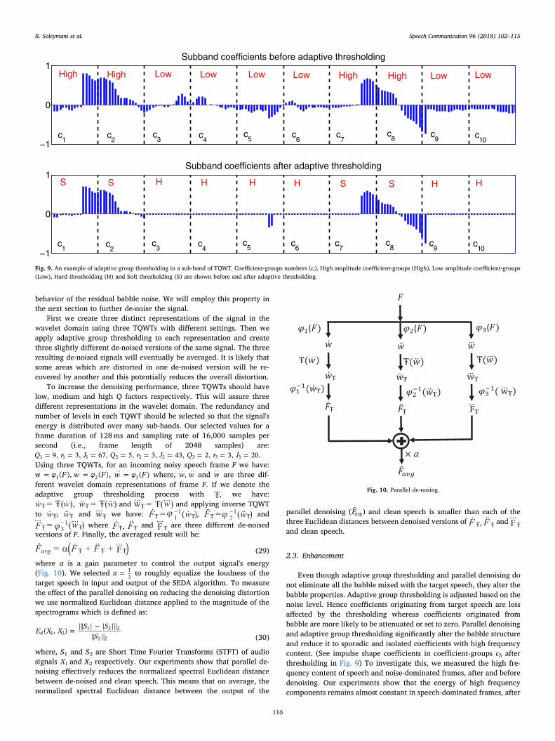
=τ 1 for speech-dominated frames and =τ 1.5 for noise-dominatedframes), ϵ is a reduction factor for soft thresholding which should al-ways be smaller than 1 (we selected =ϵ 0.3), γ should always be greaterthan 1 (we selected =γ 5) and ρ determines our desired overall de-noising aggressiveness which mainly depends on the overall SNR. Ourexperiments with various values for ρ shows that in noisier situations(i.e., lower SNR) where the target speech is not sufficiently strongerthan the background noise, we should select slightly smaller values for ρto avoid target speech distortion. Conversely, in higher SNRs we canselect slightly larger values for ρ which maximizes the noise reductionwithout major distortion of the target speech. As a part of the SEDAclassifier, we roughly classified the overall SNR into one of the six SNRranges listed in Table 2 as discussed in Section 2.1.5. The main purposeof that classification was to estimate the values of P(classN) and P(classS)for maximum a posteriori estimation. In addition to MAP estimation,we use this estimated SNR range to select the value of ρ in the denoisingstage (we selected =ρ 2 for overall SNR<4.5, =ρ 3 for 4.5< overallSNR<10.5 and =ρ 3.5 for overall SNR>10.5). Note that the selectedvalues for SEDA parameters are tuned for multi-talker babble noise withnumber of talkers between 4–20 and we used the same values for SEDAparameters during the listening tests described in Section 3. Fig. 9shows that soft thresholding preserves the shape of the clusters (bykeeping smaller coefficients) in speech originated high amplitudecoefficient-groups c1, c2, c7 and c8.

2.2.2. Parallel denoisingAdaptive group thresholding usually inflicts some distortion to the

original speech. We propose a parallel denoising approach to recoverthe distorted parts of the speech. Parallel denoising also changes the

R. Soleymani et al. Speech Communication 96 (2018) 102–115

109

behavior of the residual babble noise. We will employ this property inthe next section to further de-noise the signal.

First we create three distinct representations of the signal in thewavelet domain using three TQWTs with different settings. Then weapply adaptive group thresholding to each representation and createthree slightly different de-noised versions of the same signal. The threeresulting de-noised signals will eventually be averaged. It is likely thatsome areas which are distorted in one de-noised version will be re-covered by another and this potentially reduces the overall distortion.

To increase the denoising performance, three TQWTs should havelow, medium and high Q factors respectively. This will assure threedifferent representations in the wavelet domain. The redundancy andnumber of levels in each TQWT should be selected so that the signal'senergy is distributed over many sub-bands. Our selected values for aframe duration of 128ms and sampling rate of 16,000 samples persecond (i.e., frame length of 2048 samples) are:

= = = = = = = = =Q r J Q r J Q r J9, 3, 67, 5, 3, 43, 2, 3, 201 1 1 2 2 2 3 3 3 .Using three TQWTs, for an incoming noisy speech frame F we have:

= =w φ F w φ F( ), ( ).

1..

2 , =w φ F( )...

3 where, w w,. ..

and w...

are three dif-ferent wavelet domain representations of frame F. If we denote theadaptive group thresholding process with , we have:

and and applying inverse TQWTto , and we have: , and

where and are three different de-noisedversions of F. Finally, the averaged result will be:

(29)

where α is a gain parameter to control the output signal's energy(Fig. 10). We selected =α 1

3 to roughly equalize the loudness of thetarget speech in input and output of the SEDA algorithm. To measurethe effect of the parallel denoising on reducing the denoising distortionwe use normalized Euclidean distance applied to the magnitude of thespectrograms which is defined as:

= −E X X S SS

( , )d 1 21 2 2

2 2 (30)

where, S1 and S2 are Short Time Fourier Transforms (STFT) of audiosignals X1 and X2 respectively. Our experiments show that parallel de-noising effectively reduces the normalized spectral Euclidean distancebetween de-noised and clean speech. This means that on average, thenormalized spectral Euclidean distance between the output of the

parallel denoising (Favg) and clean speech is smaller than each of thethree Euclidean distances between denoised versions of andand clean speech.

2.3. Enhancement

Even though adaptive group thresholding and parallel denoising donot eliminate all the babble mixed with the target speech, they alter thebabble properties. Adaptive group thresholding is adjusted based on thenoise level. Hence coefficients originating from target speech are lessaffected by the thresholding whereas coefficients originated frombabble are more likely to be attenuated or set to zero. Parallel denoisingand adaptive group thresholding significantly alter the babble structureand reduce it to sporadic and isolated coefficients with high frequencycontent. (See impulse shape coefficients in coefficient-groups c5 afterthresholding in Fig. 9) To investigate this, we measured the high fre-quency content of speech and noise-dominated frames, after and beforedenoising. Our experiments show that the energy of high frequencycomponents remains almost constant in speech-dominated frames, after

−1

0

1Subband coefficients before adaptive thresholding

−1

0

1Subband coefficients after adaptive thresholding

c3 c

4c

5 c6

c7

c8 c

9 c10

c10

c9

c8c

7c

6c

5c4

c3c

2

c1

c2

c1

S S H H H H S S H H

LowLowHighHighLowLowLowLowHighHigh

Fig. 9. An example of adaptive group thresholding in a sub-band of TQWT. Coefficient-groups numbers (ci), High amplitude coefficient-groups (High), Low amplitude coefficient-groups(Low), Hard thresholding (H) and Soft thresholding (S) are shown before and after adaptive thresholding.

( )

( ) ( )

Ŧ( ) Ŧ( ) Ŧ()

Ŧ Ŧ wŦ

( Ŧ) ( Ŧ) ( wŦ)

Ŧ Ŧ FŦ

×

Fig. 10. Parallel de-nosing.

R. Soleymani et al. Speech Communication 96 (2018) 102–115

110

and before parallel denoising whereas it drastically increases in noise-dominated frames. To exploit the above mentioned property, afterparallel denoising we apply a suitable low-pass filter only to the noise-dominated frames to remove the high frequency residual componentsresulting from the previous denoising steps and further enhance thespeech quality. In SEDA we used a 6th order Butterworth low pass filterwith cut-off frequency of 4000 Hz.

3. Methods

The effect of SEDA on speech intelligibility and sound quality wasevaluated for cochlear implant users. IEEE sentences were presentedagainst randomly generated multi-talker background noise at SNRsbetween 0 and 9 dB with and without SEDA processing. In the firstexperiment, subjects were asked to repeat as much of each sentence asthey could understand. In the second experiment, subjects were askedto rate the sound quality of each sentence.

3.1. Subjects

Seven post-lingually deafened CI subjects were tested. None of thesubjects had usable residual hearing in either ear without amplification.Nevertheless, all subjects who used hearing aids in daily life wore foamearplugs during the experiment. Specific subject demographics aregiven in Table 4.

All subjects provided informed consent in accordance with theInstitutional Review Board at the New York University LangoneMedical Center. For all subjects, intelligibility in quiet was measured asa reference and its average was 63.6%.

3.2. IEEE Sentences in Noise Intelligibility

IEEE standard sentences (IEEE Subcommittee, 1969) with andwithout processing at SNRs of 0, 3, 6, and 9 dB were used to evaluateSEDA. As a baseline, understanding of IEEE sentences in quiet were alsoevaluated. The noise used for testing was the 10-talker (5 male and 5female speakers) babble randomly created from a database of 2100sentences (excluding the sentences which were used for training theclassifier) as described in Section 2.1.6. For each of the eight speech innoise conditions (processed and unprocessed at four different SNRs), 4sentence lists were randomly selected (without replacement) from 72male speaker IEEE standard sentence lists. An additional 2 sentence listswere also randomly selected to evaluate speech in quiet performance(i.e. with no background talkers or SEDA processing) for all subjects.The resulting 34 lists of sentences (340 sentences total) were presentedin a random order to the subject. Before starting the experiment, thesubject practiced the test using a randomly selected sentence list where

each of the sentences was presented in a different condition. Speechmaterial was played in free field in a double-walled sound booth at 65dBa. Subjects were instructed to face the loudspeaker and were posi-tioned approximately 1 m from the loudspeaker. Speech understandingwas performed using i-STAR software (TigerSpeech Technology andEmily Fu Foundation, 2015). Subjects listened using their clinical set-tings of their cochlear implant. If applicable, subjects were instructed toremove their hearing aid devices during the test and wear a foamearplug. Subjects were instructed to repeat as much of the sentence asthey could. Each sentence was presented only once. For each subject,the randomization process was repeated and new sentence lists wereassigned. Subjects’ responses were recorded and the percent correct ofall words (combined key and non-key) for each condition was calcu-lated by i-STAR. Note that i-STAR software works with databases of pre-processed audio samples. To simulate the real-time condition, we usedthe SEDA algorithm which receives and processes the noisy signal frameby frame without knowledge of the entire signal. The resulting denoisedsamples were saved for use by i-STAR for the listening test.

3.3. Sound quality rating

After evaluating each subject's understanding of IEEE sentences, thesound quality of the IEEE sentences in noise (with and without SEDAprocessing) was measured using the MUSHRA (MUltiple Stimuli withHidden Reference and Anchor) scaling test. The open sourceMUSHRAM interface (Vincent, 2005) was used to conduct the experi-ment. Subjects were presented with a reference sound, which wasspeech in quiet, and were told that the quality of this sound should berated as 100 on a scale from 0 to 100. Subjects were also presented with10 other variations of the sentence and were asked to scale the soundquality of the speech in each of those variations along the same scale.The variations consisted of the 8 speech in noise conditions previouslyevaluated for intelligibility (i.e. SNRs of 0, 3, 6, and 9 dB with andwithout SEDA processing), an unlabeled repetition of the reference(speech in quiet) and a sample with only the background babble noiseused as an anchor. Subjects were allowed to listen to each sample asmany times as desired and similarly were also able to replay the re-ference stimulus as desired to facilitate the comparison of the soundqualities. Responses for each variation were entered by the subjectusing a slider in the interface. When the subject was satisfied with his/her rating of all of the samples, he/she would press a button to save allof the values and proceed to the next set of sentences. The interfaceused is presented in Fig. 11. The process was repeated for 5 differentsentences for each subject. The sentences used were randomly selectedfor each subject from the 720 male speaker IEEE standard sentences.Speech material was played in free field in a double-walled sound boothat 65 dBa. Subjects were instructed to face the loudspeaker and were

Table 4Subject information.

Subject Age Sex Etiology Ear Implantation Year Type of implant Strategy / noise reduction

M107 61 M Unknown Left 2013 MED-EL Concert - Flex 28 FS4Right N/A N/A (Hearing Aid)a N/A

N103 60 F Genetic Left N/A N/A (Hearing Aid)a N/ARight 2008 Cochlear CI24RE (CA) ACE

C106 39 M Unknown Left N/A N/A (Hearing Aid)a N/ARight 2010 Advanced Bionics HiRes90K / HiFocus 1J HiRes-S with Fidelity 120 / ClearVoice

C114 70 F Meniere's Autoimmune Left N/A N/A (Hearing Aid)a N/ARight 2014 Advanced Bionics HiRes90K / HiFocus MS HiRes-Optima-S / ClearVoice

C118 45 F Ushers Left 2010 Advanced Bionics HiRes90K / HiFocus 1J HiRes-P with Fidelity 120 / ClearVoiceRight N/A N/A (Hearing Aid)a N/A

N102 64 F Lyme Disease and head trauma Left N/A N/A (Hearing Aid)a N/ARight 2013 Cochlear Freedom CI24RE CA ACE

C101 71 M Unknown Left N/A N/A (Hearing Aid)a N/ARight 2012 Advanced Bionics HiRes90K / HiFocus 1J HiRes-P with Fidelity 120 / ClearVoice

a Subjects were instructed to remove their hearing aid devices and insert a foam earplug during the test.

R. Soleymani et al. Speech Communication 96 (2018) 102–115

111

positioned approximately 1 m from the loudspeaker. Because subjectC118’s vision was insufficient to use the MUSHRAM interface, she wasinstructed to scale the sounds orally.

4. Results

4.1. Speech in noise intelligibility

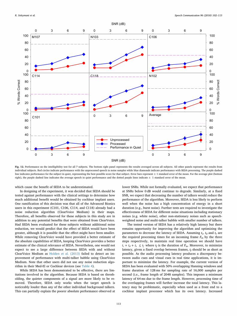
The percent of words correct for each condition is presented foreach subject in Fig. 12. As the test results show, the performance gen-erally increases as a function of SNR.

Furthermore, performance with SEDA noise reduction was higherfor all subjects at all SNRs except for C101 at 0 dB SNR, where wordrecognition was 0 for both processed and processed samples. There was,however, a great deal of variability in the magnitude of the improve-ment from SEDA noise reduction across subjects and SNRs. The averageimprovement for 0, 3, 6, and 9 dB SNR were 7.19, 11.23, 17.19, and15.96 percentage points respectively (bottom-right panel of Fig. 12). Arepeated measures two-way ANOVA detects main effects of noise re-duction [F(1,6)=31.242, p< .001] and signal to noise ratio [F(3,18)=21.090, p< .001]. Additionally, the interaction between signal to noiseratio and noise reduction is significant [F(3,18)= 10.564, p< .001].Post-hoc one-sample t-tests detected that the improvements were sig-nificant at each SNR (SNR 0 dB: t(6)= 4.605, p= .00367; SNR 3 dB: t(6)= 3.579, p= .0117; SNR 6 dB: t(6)= 5.816, p= .00113; SNR 9 dB:t(6)= 6.384, p= .000695). All four post-hoc t-tests remain significantafter Type I error correction using Rom's method (Rom, 1990) whichdetermines that if the p-value for all comparisons is below the criticalalpha, then all comparisons are considered significant. Nevertheless,there is still room for improvement with the SEDA noise reduction al-gorithm. The ideal performance for a noise reduction algorithm wouldbe to produce performance equivalent to performance in quiet (as if theall of the noise were removed without inflicting any distortion to theoriginal speech). However, even at the highest SNR tested (9 dB SNR),performance was significantly below that of performance in quiet [t(6)=11.664, p= .0000239] which is indicated by the purple dashed linesin Fig. 12.

4.2. Sound quality

Sound quality ratings for each condition are shown for each subjectin Fig. 13. As the test results show, the sound quality generally increasesas a function of SNR. Furthermore, sound quality with SEDA noise re-duction was higher for all subjects. The average increase in MUSHRAscores for 0, 3, 6, and 9 dB SNR were 12.46, 11.02, 23.55, and 28.95(bottom-right panel of Fig. 13). A repeated measures two-way ANOVAdetects main effects of noise reduction [F(1,6)= 200.070, p< .001]and signal to noise ratio [F(3,18)= 36.195, p< .001]. Additionally, asignificant interaction between noise reduction and signal to noise ratiowas detected [F(3,18)= 3.189, p=.049]. After Type I error correctionusing Rom's method (Rom, 1990), post-hoc one-sample t-tests detecteda significant improvement in sound quality at SNRs of 6 dB (t(6)=7.089, p= .000395) and 9 dB (t(6)=6.176, p= .000828). However,improvements in sound quality approached but failed to reach sig-nificance for SNR 0 dB (t(6)= 2.289, p= .0621) and SNR 3 dB (t(6)=2.932, p= .0262) after Type I error correction.

5. Discussion

Considering the particularly difficult nature of the babble noisereduction for CI devices and limited number of previous works in thisfield, babble noise reduction is a worthwhile area for CI research. SEDAis an effort to address the babble problem for cochlear implant users. Itprovides intelligibility and sound quality benefits for CI users in babblenoise environments by employing a new approach. SEDA uses a clas-sifier which is specifically tuned for multi-talker babble. It also employsa new wavelet-based approach combined with parallel denoising formulti-talker babble noise reduction in cochlear implant devices.

The evaluation of SEDA suggests that it can improve both the in-telligibility and sound quality of speech in the presence of multi-talkerbabble for CI listeners. Although post-hoc tests showed an improvementin intelligibility at all SNRs, after Type I error control, significant im-provements in sound quality were only detected for SNRs of 6 and 9 dB.Although SEDA was effective at 0 dB SNR, the improvements in in-telligibility and sound quality increased with larger SNRs. The smallerobserved improvements in intelligibility at lower SNRs are expected tobe partially caused by floor effects at lower SNRs (e.g. C101 and C114)

Fig. 11. Capture of the user interface for the MUSHRA experiment.

R. Soleymani et al. Speech Communication 96 (2018) 102–115

112

which cause the benefit of SEDA to be underestimated.In designing of the experiment, it was decided that SEDA should be

tested against performance with the clinical settings to determine howmuch additional benefit would be obtained by cochlear implant users.One ramification of this decision was that all of the Advanced Bionicsusers in this experiment (C101, C106, C114, and C118) already had anoise reduction algorithm (ClearVoice Medium) in their maps.Therefore, all benefits observed for these subjects in this study are inaddition to any potential benefits that were obtained from ClearVoice.Had SEDA been evaluated for these subjects without additional noisereduction, we would predict that the effect of SEDA would have beengreater, although it is possible that the effect might have been smaller.While removing ClearVoice would have provided a better estimate ofthe absolute capabilities of SEDA, keeping ClearVoice provides a betterestimate of the clinical relevance of SEDA. Nevertheless, one would notexpect to see a large difference between SEDA with and withoutClearVoice Medium as Holden et al. (2013) failed to detect an im-provement of performance with multi-talker babble using ClearVoiceMedium. Note that other users did not use any noise reduction algo-rithm in their Med-El or Cochlear devices (see Table 4).

While SEDA has been demonstrated to be effective, there are lim-itations involved in the algorithm. Because SEDA is based on thresh-olding, the quieter components of a signal are more likely to be re-moved. Therefore, SEDA only works when the target speech isnoticeably louder than any of the other individual background talkers.This can partially explain the poorer absolute performance observed at

lower SNRs. While not formally evaluated, we expect that performanceat SNRs below 0 dB would continue to degrade. Similarly, at a fixedSNR, we expect that decreasing the number of talkers would reduce theperformance of the algorithm. Moreover, SEDA is less likely to performwell when the noise has a high concentration of energy in a shortduration (e.g., burst noise). Further tests are required to investigate theeffectiveness of SEDA for different noise situations including stationarynoises (e.g. white noise), other non-stationary noises such as speech-weighted noise and multi-talker babble with smaller number of talkers.

The tested version of SEDA has a relatively high latency but thereremains opportunity for improving the algorithm and optimizing theparameters to decrease the latency of SEDA. Assuming tc, td and te arethe required processing times for an incoming frame Fin by the threesteps respectively, to maintain real time operation we should have

+ + ≤t t t tc d e f where tf is the duration of Fin. Moreover, to minimizelatency, given a fixed overlap between frames, tf should be as short aspossible. As the audio processing latency produces a discrepancy be-tween audio cues and visual cues in real time applications, it is im-portant to minimize the latency. For example, the current version ofSEDA has been evaluated with 50% overlapping Hanning windows andframe duration of 128ms for sampling rate of 16,000 samples persecond (i.e., frame length of 2048 samples). This imposes a minimumlatency of 64ms due to the frame length. However, processing time ofthe overlapping frames will further increase the total latency. This la-tency may be problematic, especially when used as a front end to acochlear implant processor which has its own latency. Increased

M107

0 3 6 9

0

20

40

60

80

100 N103

SNR (dB)

0 3 6 9

C106

0 3 6 9

0

20

40

60

80

100

C114

% W

ords

Cor

rect

0

20

40

60

80

100

UnprocessedProcessedPerformance in Quiet

C118

SNR (dB)

0 3 6 9

N102

% W

ords

Cor

rect

0

20

40

60

80

100

C101

0 3 6 9

0

20

40

60

80

100 Average

0 3 6 9

0

20

40

60

80

100

Fig. 12. Performance on the intelligibility test for all 7 subjects. The bottom right panel represents the results averaged across all subjects. All other panels represent the results fromindividual subjects. Red circles indicate performance with the unprocessed speech in noise samples while blue diamonds indicate performance with SEDA processing. The purple dashedline indicates performance for the subject in quiet, representing the best possible score for that subject. Error bars represent± 1 standard error of the mean. For the average plot (bottomright), the purple dashed line indicates the average speech in quiet performance and the dotted purple lines indicate± 1 standard error of the mean.

R. Soleymani et al. Speech Communication 96 (2018) 102–115

113

latencies can cause a disassociation between visual and auditory stimuli(e.g. Stevenson et al., 2012). The frame length could be reduced to asmaller number of samples to reduce latency. However, the effects ofshorter frame lengths on performance have yet to be evaluated. Foroptimal results with a shorter time window, the SEDA classifier wouldneed to be re-optimized accordingly. Note that a smaller number ofTQWT levels (sub-bands) should be selected for shorter frames whileother TQWT parameters (Q factors and redundancy) could remain un-changed.

Using different frame lengths for the classifier and denoising stagesalso can potentially reduce the latency of SEDA. In the present im-plementation, the frame length limitation is mainly due to the SEDAclassifier as the effectiveness of features degrades rapidly with shorterframes. However, the denoising stage can be implemented using ashorter frame length and might be less susceptible to the shortening offrame length than the classifier. Because the frame length used fordenoising stage determines the SEDA latency, using shorter frames fordenoising and longer frames for classifier would reduce the SEDA la-tency. However, further investigation is required to evaluate the effectof reducing the frame length in the denoising stage on performance.Note that having different frame lengths for classifier and denoisingstages requires modification of the SEDA algorithm.

Performance of the SEDA classifier might be enhanced for shorterframes by using additional features which are sensitive to the level ofbabble in speech, have a relatively low computational cost, and performwell for short frames of the noisy speech. For example, kurtosis-based

features, as used in Hazrati et al. (2013), might be beneficial for a futureversion of the SEDA classifier.

The evaluation of SEDA is promising for CI users, especially in thecontext of previous work. Nevertheless, because of differences in sub-ject population, difficulty of varying sentence corpuses, language, andtesting methods, it is inappropriate to directly compare results of SEDAwith other noise reduction algorithms. Further research in which eachof the above factors are controlled is needed if a direct comparisonbetween noise reduction algorithms is to be made.

The implementation of SEDA evaluated in the present manuscriptwas implemented on a Windows computer in a sound booth. However,for SEDA to be beneficial to cochlear implant users in their daily life,SEDA needs to be implemented on a smaller platform. Ideally, SEDAwould be implemented directly into the sound processor. An alternativewould be to use a smartphone as an external pre-processor to clean upthe signal using SEDA and stream the signal into the sound processor.

Acknowledgments

We appreciate the efforts of all of subjects who provided their va-luable time. The authors also thank Natalia Stupak for coordinating thetests. Support for this research was provided by the National Institutesof Health/National Institute on Deafness and Other CommunicationDisorders (R01 DC012152; PI: Landsberger) as well as an NYU School ofMedicine Applied Research Support Fund internal grant.

M107

0 3 6 9

0

20

40

60

80

100 N103

SNR (dB)

0 3 6 9

C106

0 3 6 9

0

20

40

60

80

100

C114

MU

SH

RA

Sou

nd Q

ualit

y S

core

0

20

40

60

80

100

UnprocessedProcessed

C118

SNR (dB)

0 3 6 9

N102

MU

SH

RA

Sou

nd Q

ualit

y S

core

0

20

40

60

80

100

C101

0 3 6 9

0

20

40

60

80

100 Average

0 3 6 9

0

20

40

60

80

100

Fig. 13. Performance on the MUSHRA sound quality test for all 7 subjects. The bottom right panel represents the results averaged across all subjects. All other panels represent the resultsfrom individual subjects. Red circles indicate performance with the unprocessed speech in noise samples while blue diamonds indicate performance with SEDA processing. Error barsrepresent± 1 standard error of the mean.

R. Soleymani et al. Speech Communication 96 (2018) 102–115

114

References

Bello J.P. Spring 2016. EL9173 selected topics in signal processing: audio content analysis[Online] http://www.nyu.edu/classes/bello/ACA.html.

Bentler, R., Chiou, L.K., 2006. Digital noise reduction: an overview. Trends Amplification10, 67–82.

Bilger, R.C., Nuetzel, J.M., Rabinowitz, W.M., Rzeczkowski, C., 1984. Standardization of atest of speech perception in noise. J. Speech Hear Res. 27, 32–48.

Bishop, C.M., 2007. Pattern Recognition and Machine Learning. Springer.Chung, K., Zeng, F.G., Waltzman, S., 2004. Utilizing advanced hearing aid technologies as

pre-processors to enhance cochlear implant performance. Cochlear Implants Int. 5(Suppl 1), 192–195.

Dawson, P.W., Mauger, S.J., Hersbach, A.A., 2011. Clinical evaluation of signal-to-noiseratio-based noise reduction in Nucleus(R) cochlear implant recipients. Ear Hear 32,382–390.

Duda, R.O., Hart, P.E., Stork, D.G., 2001. Pattern Classification, 2nd ed. Wiley, New York.Fetterman, B.L., Domico, E.H., 2002. Speech recognition in background noise of cochlear

implant patients. Otolaryngol. Head Neck Surg. 126, 257–263.Friedland, D.R., Runge-Samuelson, C., Baig, H., Jensen, J., 2010. Case-control analysis of

cochlear implant performance in elderly patients. Arch. Otolaryngol. Head NeckSurg. 136, 432–438.

Goehring, T., Bonler, F., Monaghan, J.J.M., van Dijk, B., Zarowski, A., Bleeck, S., 2016.Speech enhancement based on neural networks improves speech intelligibility innoise for cochlear implant users. Hearing Res. 344, 183–194.

Gu Q., Li Z., Han J. 2012. Generalized Fisher Score for feature selection. arXiv preprintarXiv:1202.3725.

Hazrati, O., Lee, J., Loizou, P.C., 2013. Blind binary masking for reverberation suppres-sion in cochlear implants. J. Acoust. Soc. Am. 133, 1607–1614.

Healy, E.W., Yoho, S.E., Wang, Y., Wang, D., 2013. An algorithm to improve speech re-cognition in noise for hearing-impaired listeners. J. Acoust. Soc. Am. 134,3029–3038.

Holden, L.K., Brenner, C., Reeder, R.M., Firszt, J.B., 2013. Postlingual adult performancein noise with HiRes 120 and clearvoice low, medium, and high. Cochlear ImplantsInt. 14, 276–286.

Hu, Y., Loizou, P.C., Li, N., Kasturi, K., 2007. Use of a sigmoidal-shaped function for noiseattenuation in cochlear implants. J. Acoust. Soc. Am. 122 EL128-34.

IEEE Recommended Practice for Speech Quality Measurements, in IEEE No 297-1969, pp.1–24, June 11 1969 doi:10.1109/IEEESTD.1969.7405210.

Kasturi, K., Loizou, P.C., 2007. Use of S-shaped input-output functions for noise sup-pression in cochlear implants. Ear Hear 28, 402–411.

Kohavi, R., 1995. A study of cross-validation and bootstrap for accuracy estimation andmodel selection. In: Proceedings of the 14th International Joint Conference OnArtificial Intelligence. Montreal, Quebec, Canada. 2. Morgan Kaufmann PublishersInc., pp. 1137–1143.

Krishnamurthy, N., Hansen, J.H.L., 2009. Babble noise: modeling, analysis, and appli-cations. IEEE Trans. Audio, Speech, Lang. Process. 17, 1394–1407.

Loizou, P.C., Lobo, A., Hu, Y., 2005. Subspace algorithms for noise reduction in cochlearimplants. J. Acoust. Soc. Am. 118, 2791–2793.

Mauger, S.J., Arora, K., Dawson, P.W., 2012. Cochlear implant optimized noise reduction.J. Neural Eng. 9, 065007.

Muller-Deile, J., Schmidt, B.J., Rudert, H., 1995. Effects of noise on speech discriminationin cochlear implant patients. Ann. Otol. Rhinol. Laryngol. Suppl. 166, 303–306.

Nilsson, M., Soli, S.D., Sullivan, J.A., 1994. Development of the hearing in noise test forthe measurement of speech reception thresholds in quiet and in noise. J. Acoust. Soc.Am. 95, 1085–1099.

Powers, D.M.W., 2011. Evaluation: from precision, recall and F-measure to ROC, in-formedness, markedness & correlation. J. Mach. Learn. Technol. 2, 37–63.

Reynolds, D., 2009. Gaussian Mixture Models. In: Li, S.Z., Jain, A. (Eds.), Encyclopedia ofBiometrics. Springer US, pp. 659–663.

Reynolds, D.A., Quatieri, T.F., Dunn, R.B., 2000. Speaker verification using adaptedgaussian mixture models. Digit. Signal Process. 10, 19–41.

Roland Jr., J.T., Gantz, B.J., Waltzman, S.B., Parkinson, A.J., Multicenter Clinical Trial,G., 2016. United States multicenter clinical trial of the cochlear nucleus hybrid im-plant system. Laryngoscope 126, 175–181.

Rom, D.M., 1990. A sequentially rejective test procedure based on a modified Bonferroniinequality. Biometrika 77, 663–665. http://dx.doi.org/10.1093/biomet/77.3.663.

Selesnick, I.W., 2010. A new sparsity-enabled signal separation method based on signalresonance. In: 2010 IEEE International Conference on Acoustics, Speech and SignalProcessing, pp. 4150–4153.

Selesnick I.W. 2011a. Sparse signal representations using the tunable Q-factor wavelettransform, Vol. 8138. pp. 81381U-81381U-15.

Selesnick, I.W., 2011b. Wavelet transform with tunable Q-factor. IEEE Trans. SignalProcess. 59, 3560–3575.

Shlens J. 2003. A tutorial on principal component analysis.Sperry, J.L., Wiley, T.L., Chial, M.R., 1997. Word recognition performance in various

background competitors. J. Am. Acad. Audiol. 8, 71–80.Stevenson, R.A., Zemtsov, R.K., Wallace, M.T., 2012. Individual differences in the mul-

tisensory temporal binding window predict susceptibility to audiovisual illusions. J.Exp. Psychol. Hum. Percept. Perform. 38, 1517–1529.

Swets, J.A., 1988. Measuring the accuracy of diagnostic systems. Science 240,1285–1293.

Tang, J., Aleyani, S., Liu, H., 2014. Feature Selection for Classification: A Review, DataClassification: Algorithms and Applications. CRC Press.

TigerSpeech Technology and Emily Fu Foundation. 2015. Internet-based speech testing,Assessment, & Recognition [Online] http://istar.emilyfufoundation.org/.

Toledo, F., Loizou, P., Lobo, A., 2003. Subspace and envelope subtraction algorithms fornoise reduction in cochlear implants, engineering in medicine and biology society,2003. In: Proceedings of the 25th Annual International Conference of the IEEE. Vol.3. pp. 2002–2005 Vol. 3.

Vincent E. 2005. MUSHRAM: a MATLAB interface for MUSHRA listening tests [Online]https://members.loria.fr/EVincent/software-and-data/ (verified August 2nd, 2016).

Yang, L.P., Fu, Q.J., 2005. Spectral subtraction-based speech enhancement for cochlearimplant patients in background noise. J. Acoust. Soc. Am. 117, 1001–1004.

Ye, H., Deng, G., Mauger, S.J., Hersbach, A.A., Dawson, P.W., Heasman, J.M., 2013. Awavelet-based noise reduction algorithm and its clinical evaluation in cochlear im-plants. PLoS One 8, e75662.

Yue, H.H., Tomoyasu, M., 2004. Weighted principal component analysis and its appli-cations to improve FDC performance, Decision and Control, 2004. In: CDC. 43rd IEEEConference on. Vol. 4. pp. 4262–4267 Vol. 4.

R. Soleymani et al. Speech Communication 96 (2018) 102–115

115