sediment plume modelling...sediment plume modelling appendix b model-measurement comparisons 97...
TRANSCRIPT

Sediment Plume Modelling Prepared for Trans-Tasman Resources Ltd
October 2015

© All rights reserved. This publication may not be reproduced or copied in any form without the permission of the copyright owner(s). Such permission is only to be given in accordance with the terms of the client’s contract with NIWA. This copyright extends to all forms of copying and any storage of material in any kind of information retrieval system.
Whilst NIWA has used all reasonable endeavours to ensure that the information contained in this document is accurate, NIWA does not give any express or implied warranty as to the completeness of the information contained herein, or that it will be suitable for any purpose(s) other than those specifically contemplated during the Project or agreed by NIWA and the Client.
Prepared by: Mark Hadfield Helen Macdonald
For any information regarding this report please contact:
Mark Hadfield Marine Physics Modeller Marine Physics +64-4-386 0363 [email protected]
National Institute of Water & Atmospheric Research Ltd
Private Bag 14901
Kilbirnie
Wellington 6241
Phone +64 4 386 0300
NIWA CLIENT REPORT No: WLG2015-22 Report date: October 2015 NIWA Project: TTR16301
Quality Assurance Statement
Dr Graham Rickard Reviewed by:
P Allen Formatting checked by:
Dr Alison MacDiarmid Approved for release by:

Sediment Plume Modelling
Contents
Executive summary ............................................................................................................. 8
1 Introduction ............................................................................................................ 10
1.1 Oceanographic conditions ...................................................................................... 11
2 Model setup ............................................................................................................ 14
2.1 Nested grids ............................................................................................................ 14
2.2 Outer (Cook Strait) model ....................................................................................... 14
2.3 Inner (sediment) model .......................................................................................... 18
2.4 Sediment model setup ............................................................................................ 19
2.5 River inputs ............................................................................................................. 22
2.6 Sediment model setup ............................................................................................ 25
2.7 Sediment properties and release parameters ........................................................ 25
2.8 Background sediments ........................................................................................... 25
2.9 Mining-derived sediments ...................................................................................... 26
3 Hydrodynamic model evaluation .............................................................................. 30
3.1 Field measurements ............................................................................................... 30
3.2 Tidal current comparison ........................................................................................ 30
3.3 Sub-tidal current comparison ................................................................................. 33
4 Sediment model evaluation ..................................................................................... 38
4.1 Surface SSC comparison with in situ measurements .............................................. 38
4.2 Surface SSC comparison with remote-sensed data ................................................ 41
4.3 Near-bottom SSC comparison with in situ ABS data .............................................. 44
5 Sediment model results ........................................................................................... 47
5.1 Suspended source at mining location A ................................................................. 47
5.2 Suspended source at mining location B .................................................................. 70
5.3 Patch source............................................................................................................ 87
6 Acknowledgements ................................................................................................. 91
7 References ............................................................................................................... 92
Appendix A The ROMS vertical grid ..................................................................... 96

Sediment Plume Modelling
Appendix B Model-measurement comparisons ................................................... 97
Appendix C Comparison with March 2014 model results ................................... 106
Tables
Table 2-1: Rivers represented in the inner model, with mean freshwater and sediment input rates from WRENZ. 22
Table 2-2: Background sediment parameters. 26
Table 2-3: Suspended source sediment parameters. 27
Table 2-4: Summary of changes in discharge rates for the finer mining-derived sediments. 27
Table 2-5: Patch sediment parameters. 29
Table 3-1: ADCP data availability from the field measurements. 30
Table A-1: Inner model layer thicknesses. 96
Table B-1: Comparison of Mtidal ellipse parameters. 99
Table B-2: Mid-depth sub-tidal velocity comparison. 103
Table B-3: Near-surface subtidal velocity comparison. 104
Table B-4: Near-bottom subtidal velocity comparison. 105
Figures
Figure 1-1: Location map. 11
Figure 1-2: Peak velocity of the net tidal current 12
Figure 1-3: Spatial distribution of mean wave energy flux. 13
Figure 1-4: Wind rose from measurements at Hawera over a period of 8 years (January 2004 to July 2012). 13
Figure 2-1: ROMS model domains. 15
Figure 2-2: Surface circulation around New Zealand. 16
Figure 2-3: Time-averaged, depth-average velocity from the Cook Strait model. 18
Figure 2-4: Time-averaged, depth-average velocity from the inner (sediment) model. 18
Figure 2-5: Bottom boundary layer & sediment bed time series at instrument site 7. 21
Figure 2-6: Daily average SSC vs flow for Whanganui River. 23
Figure 2-7: Near-bottom speeds (m s−1) on the inner model domain. 24
Figure 3-1: M2 tidal velocity comparison (ADCP Site 7 Deployment 2). 31
Figure 3-2: M2 tidal current profile comparison (ADCP Site 7 Deployment 2). 32
Figure 3-3: Tidal velocity comparison for S2, N2 and K1 (ADCP Site 7 Deployment 2). 33
Figure 3-4: Sub-tidal velocity comparison (ADCP Site 7 Deployment 2). 35
Figure 3-5: Comparison of detiding methods (ADCP Site 7 Deployment 2). 36
Figure 4-1: SSC time series at near-shore site 11 (Whanganui). 39
Figure 4-2: SSC time series at near-shore site 12 (Kai Iwi). 39
Figure 4-3: SSC time series at near-shore site 13 (Waitotara River). 39
Figure 4-4: SSC time series at near-shore site 14 (Patea). 40
Figure 4-5: SSC time series at near-shore site 15 (Manawapou). 40

Sediment Plume Modelling
Figure 4-6: SSC time series at near-shore site 16 (Ohawe). 40
Figure 4-7: Modelled and observed 5th percentile surface concentration of background sediment. 42
Figure 4-8: Modelled and observed median (50th percentile) surface concentration of background sediment. 43
Figure 4-9: Modelled and observed 95th percentile surface concentration of background sediment. 43
Figure 4-10: Time series of near-bottom sand concentration at instrument site 6. 45
Figure 4-11: Time series of near-bottom sand concentration at instrument site 7. 45
Figure 4-12: Time series of near-bottom sand concentration at instrument site 8. 45
Figure 4-13: Time series of near-bottom sand concentration at instrument site 10. 46
Figure 5-1: Surface plume Case 1 (suspended source at location A). 48
Figure 5-2: Vertical structure of the plume in Case 1 (suspended source at location A). 49
Figure 5-3: Surface plume and vertical transect for Case 2 (suspended source at location A). 50
Figure 5-4: Surface plume and vertical transect for Case 3 (suspended source at location A). 51
Figure 5-5: Surface plume and vertical transect for Case 4 (suspended source at location A). 52
Figure 5-6: Surface plume and vertical transect for Case 5 (suspended source at location A). 53
Figure 5-7: Surface plume and vertical transect for Case 6 (suspended source at location A). 54
Figure 5-8: Median near-surface concentration of suspended sediment from mining at source location A. 57
Figure 5-9: 99th percentile near-surface concentration of suspended sediment from mining (50 Mt/a) at source location A. 58
Figure 5-10: Median near-bottom concentration of suspended sediment from mining (50 Mt/a) at source location A. 59
Figure 5-11: 99th percentile near-bottom concentration of suspended sediment from mining (50 Mt/a) at source location A. 60
Figure 5-12: Near-source statistics of mining derived sediment concentration from mining source A. 61
Figure 5-13: Median summer (December–February) near-surface concentration of suspended sediment from mining (50 Mt/a) at source location A. 63
Figure 5-14: Median winter (July–August) near-surface concentration of suspended sediment from mining (50 Mt/a) at source location A. 64
Figure 5-15: Maximum 5-day increment in sediment bed thickness for suspended sediment from mining source A. 66
Figure 5-16: Maximum 365-day increment in sediment bed thickness for suspended sediment from mining source A. 67
Figure 5-17: Near-source maximum increment of mining derived sediment, source A. 68
Figure 5-18: 2-year increment in sediment bed thickness for suspended sediment from mining source A. 69
Figure 5-19: Surface plume and vertical transect for Case 1 (suspended source at location B). 71
Sediment Plume Modelling
Figure 5-20: Surface plume and vertical transect for Case 2 (suspended source at location B). 72
Figure 5-21: Surface plume and vertical transect for Case 3 (suspended source at location B). 73
Figure 5-22: Surface plume and vertical transect for Case 4 (suspended source at location B). 74
Figure 5-23: Surface plume and vertical transect for Case 5 (suspended source at location B). 75
Figure 5-24: Surface plume and vertical transect for case61 (suspended source at location B). 76
Figure 5-25: Median near-surface concentration of suspended sediment from mining at source location B. 78
Figure 5-26: 99th percentile near-surface concentration of suspended sediment from mining at source location B. 79
Figure 5-27: Median near-bottom concentration of suspended sediment from mining at source location B. 80
Figure 5-28: 99th percentile near-bottom concentration of suspended sediment from mining at source location B. 81
Figure 5-29: Near-source statistics of mining derived sediment concentration from mining source B. 82
Figure 5-30: Maximum 5-day increment in sediment bed thickness for suspended sediment from mining source B. 84
Figure 5-31: Maximum 365-day increment in sediment bed thickness for suspended sediment from mining source B. 85
Figure 5-32: Near-source maximum increment of mining derived sediment, source B. 86
Figure 5-33: Thickness of fine sediment from the patch source. 88
Figure 5-34: 99th percentile of near-surface SSC of fine sediments from the patch. 89
Figure 5-35: 99th percentile of near-bottom SSC of fine sediments from the patch. 90
Figure A-1: ROMS vertical grid schematic. 96
Figure B-1: Tidal ellipse comparison (all ADCP deployments). 97
Figure B-2: Tidal profile comparison (all ADCP deployments). 98
Figure B-3: Sub-tidal variance ellipse comparison (all ADCP deployments). 100
Figure B-4: Sub-tidal along-axis velocity comparison (all ADCP deployments). 101
Figure B-5: Sub-tidal across-axis velocity comparison (all ADCP deployments). 102
Figure C-1: Comparison of median near-surface SSC due to mining at source location A. 106
Figure C-2: Comparison of 99th percentile near-surface SSC due to mining at source location A. 107
Figure C-3: Comparison of median near-bottom SSC due to mining at source location A. 108
Figure C-4: Comparison of 99th percentile near-bottom SSC due to mining at source location A. 109
Figure C-5: Comparison of median near-surface SSC due to mining at source location B. 110
Figure C-6: Comparison of 99th percentile near-surface SSC due to mining at source location B. 111
Sediment Plume Modelling
Figure C-7: Comparison of median near-bottom SSC due to mining at source location B. 112
Figure C-8: Comparison of 99th percentile near-bottom SSC due to mining at source location B. 113
Figure C-9: Maximum 5-day increment in sediment bed thickness for suspended sediment due to mining at source location A. 114
Figure C-10: Maximum 365-day increment in sediment bed thickness for suspended sediment due to mining at source location A. 115
Figure C-11:: Maximum 5-day increment in sediment bed thickness for suspended sediment due to mining at source location B. 116
Figure C-12: Maximum 365-day increment in sediment bed thickness for suspended sediment due to mining at source location B. 117

8 Sediment Plume Modelling
Executive summary Trans-Tasman Resources Ltd (TTR) proposes to extract titanomagnetite sand (ironsand) from an area
in South Taranaki Bight. NIWA was commissioned by TTR to investigate potential environmental
impacts of the proposed extraction operation. The operation will result in suspended-sediment
plumes and sediment deposition on the seabed. It is recognised that this will have an impact on the
ocean environment.
Following the refusal of consent for an earlier application in June 2014, TTR re-assessed their
scientific case as background for a second application. A detailed review and a subsequent test
program by HR Wallingford Ltd (HRW) has allowed for more accurate modelling of the plume by
addressing the following aspects:
Flocculation: The original plume model neglected flocculation, a process in which fine
sediment particles combine into fast-sinking aggregates, called flocs;
Sediment settling rates: The extent to which the fine suspended sediment would settle
to the bottom and be trapped in the matrix of discharged sand has been reviewed by
HR Wallingford and is predicted to occur to a greater extent than assumed previously.
Sediment resuspension: The HR Wallingford tests found that the shear stress required
for resuspension of freshly deposited material was in the range 0.2–0.3 Pa rather than
the 0.1 Pa (minimum value) assumed by NIWA.
The output of sediment from the ironsand extraction operation is represented with two sources:
The suspended source, representing fine sediment (grain size < 63 µm) introduced into
suspension via two discharge streams: the overflow from the hydro-cyclone
dewatering system and the de-ored sand discharge;
The patch source, an area of 3 × 2 km representing one year’s discharge of de-ored
sand, including trapped fine material.
Of these, the suspended source has by far the greater impact in terms of the extent and magnitude
of the concentrations in the sediment plume.
Two source locations are considered, at the inner end (A) and the outer end (B) of the project area.
These two points represent the limits of inshore and offshore mining locations within the proposed
project area.
The suspended source was introduced in a simulation of 1000 days duration, with the source
operating for the final 800 days (with 20% down-time) and statistics calculated over the final two
years. The analysis of suspended sediment concentrations (SSC) focussed on the median and 99th
percentile, comparing values for background sediments, mining-derived sediments and the
combination of the two.
Plumes from the suspended source generally extend to the east-southeast as a result of the
prevailing winds and residual currents. Occasionally the plume will pool around the mining areas or
move towards the west or south in response to changed wind patterns which affect the prevailing
currents. The envelope of the area predicted to be impacted by the plume over the course of the
simulated release has been established. The plume envelope from the inshore source, location A,
shows that the plume influences the coast between Patea and Whanganui with very low

Sediment Plume Modelling 9
concentrations, substantially (around 100 times) less than the naturally occurring background
concentrations, following the coast towards Kapiti. The highest surface concentrations associated
with the plume occur at the source location and are 1.45 mg/L (median) and 8.2 mg/L (99th
percentile). At 20 km downstream from the source the surface concentrations reduce to 0.35 mg/L
(median) and 2.8 mg/L (99th percentile). The plume envelope for the offshore source location B is
located further offshore but follows a similar path to the east-southeast, with the concentrations
being significantly lower than for source location A. In both cases the plume of mining-derived
sediment contributes noticeably to the total SSC within a few kilometres of the source but is
insignificant relative to the background SSC near the coast.
An analysis of mining-derived and background SSCs for the suspended source at location A in
summer (December–February) and winter (July–August) indicates that both mining-derived and
background concentrations are lower in summer than winter. The net effect is that the mining-
derived plume is somewhat more pronounced relative to the background in summer than in winter.
Deposition from the suspended source has been characterised by two statistics, the maximum 5-day
deposition (i.e. the maximum amount of material predicted to accumulate over any 5-day interval)
and the maximum 365-day deposition. As defined by these statistics, the deposition footprint of
mining-derived sediment is widespread but at very low values of 0.01–0.05 mm, i.e. one-tenth the
thickness of a human hair (typically 0.1 mm). The deposition of mining derived sediment would only
be able to be distinguished from the background within a few kilometres of the source.
With the patch source, fine sediments trapped in the pit are eroded, transported and deposited, but
only at a low rate, forming a deposition footprint (> 0.01 mm) that extends up to 10 km from the
patch boundary after two years. Suspended sediment concentrations in the associated plume are
small relative to background SSCs.
10 Sediment Plume Modelling
1 Introduction Trans-Tasman Resources Ltd (TTR) proposes to extract titanomagnetite sand (ironsand) from an area
in South Taranaki Bight (Figure 1-1). The plan defines a project area in a roughly triangular region at
20–40 m depth off the South Taranaki coast near Patea. On hydrographic charts parts of this area are
labelled Whenuakura Spur, Graham Bank, Patea Banks and The Rolling Ground. Here the area as a
whole will be called the Patea Shoals.
As input to the Environmental Impact Assessment (EIA) for the proposal NIWA was commissioned by
TTR to investigate the potential impacts of the proposed extraction operation. The set of sediment
plume model results presented to the Decision Making Committee (as revised in March 2014) will be
called the March 2014 configuration.
Following the refusal of consent by the Decision Making Committee in June 2014, TTR re-assessed
their scientific case as background for a second application. One issue that arose was the need to
provide more certainty and accuracy in the sediment plume modelling studies and the interpretation
of these results. In July 2014 HR Wallingford undertook a structured review of the NIWA sediment
plume modelling work which included a detailed assessment of the assumptions and inputs.
The March 2014 NIWA plume modelling assumed that the material discharged into the sea would
remain in its particulate (unflocculated) form. The HR Wallingford tests indicated that most of the
fine sediment in the tailings would exist in the environment in flocculated form and would therefore
settle from the upper part of the water column more quickly than assumed in the NIWA sediment
plume modelling. The HR Wallingford tests also found that the shear stress for resuspension of
freshly deposited material was in the range 0.2–0.3 Pa rather than the 0.1 Pa (minimum value) as
assumed by NIWA. HR Wallingford also addressed the trapping of mining-derived fine sediment in
the matrix of coarser tailings in the mining pit, using a high resolution 3D flow and sediment
transport model.
The present report presents a more accurate sediment plume model incorporating the confirmed
sediment settling parameters and source rates from the HR Wallingford work (HR Wallingford 2015).

Sediment Plume Modelling 11
Figure 1-1: Location map. The proposed mining area is shaded red. The solid black rectangle outlines the inner model domain (Cape Egmont to Kapiti) on which the sediment model was set up, as described in Section 2. The orange line indicates the boundary of the territorial sea. Also shown are the towns and villages and the mouths of the principal rivers along the Taranaki and Manawatu coasts. Stars indicate named offshore oil/gas production platforms.
1.1 Oceanographic conditions
The movement of sediments in the vicinity of the proposed mining area is heavily influenced by
physical conditions. This section briefly describes the background physical conditions that influence
water and sediment movement. More detailed descriptions can be found in earlier reports
(MacDiarmid et al. 2010; MacDonald et al. 2012).
Tidal currents are typically strong in this area, due to the difference in tidal phase between the
western and eastern ends of Greater Cook Strait Figure 1-2 shows tidal velocities from the NIWA tidal
model (Goring 2001; Goring et al. 1997; Walters et al. 2001). The tidal flow amplitude exceeds 1 m/s
in Cook Strait Narrows. Over Patea Shoals the tidal flows are around 0.4 m/s and are largely parallel
to the shore.

12 Sediment Plume Modelling
Figure 1-2: Peak velocity of the net tidal current The maximum speed is shown by the colour scale, while maximum and minimum velocity vectors are shown by the longer and shorter of the crossed arrows, respectively. Figure from MacDiarmid et al. 2010.
The wave energy flux across the 50 m isobath from a 20 year hindcast (Gorman et al. 2003a, Gorman
et al. 2003b) is shown in Figure 1-3. The prevailing wave swell direction tends to be from the south-
west; as such, the wave energy flux is typically higher in the north-west part of the domain than the
more sheltered south-east. The wave energy fluxes are not normal to the coastline in the domain,
with the shore-parallel flux typically toward the south-east along the northerly part of the shoreline,
while the flux has a northerly component along the eastern shoreline. This flux influences the
distribution of sediment. The significant wave height statistics from the hindcast show that the north
of the region has a mean peak at around 1.5 m, but that heights in excess of 8 m also arise, especially
in the winter months during storm events. In the relatively sheltered eastern part of the domain, the
mean heights are around 1 m, and the maximum wave heights are generally less than 6 m or so.
Wave periods are typically in the range 10–14 s.
A wind rose for 8 years of observations at Hawera between January 2004 and July 2012 is shown in
Figure 1-4. Winds are predominantly from the north, southeast and west. The mean wind speed is
5.3 m/s and the maximum over the period was 21.1 m/s on 15 February 2004.

Sediment Plume Modelling 13
Figure 1-3: Spatial distribution of mean wave energy flux. This is the distribution of the flux along the 50 m isobath averaged over the full 20-year hindcast record. The colour scale shows the mean of the magnitude of the energy flux, while the arrows show the vector averaged flux. Figure from MacDiarmid et al. 2010.
Figure 1-4: Wind rose from measurements at Hawera over a period of 8 years (January 2004 to July 2012). Meteorological convention is used in expressing the direction that the wind blows from. Figure from MacDonald et al. 2012.

14 Sediment Plume Modelling
2 Model setup
2.1 Nested grids
Sediment plume behaviour was predicted using a modelling system comprising a set of nested
domains. The outer domain covered Greater Cook Strait (Figure 2-1). Two different inner domains
were defined and used in different simulations, a larger domain extending from Cape Egmont to just
north of Kapiti Island and another covering a smaller area over Patea Shoals. The model was ROMS
(Haidvogel et al. 2008), a widely accepted ocean/coastal model with optional embedded models of
suspended-sediment and sediment-bed processes (Warner et al. 2008). In all cases the inner domain
is the one on which sediment processes are simulated.
In the model nesting procedure, the outer domain model provides time-varying lateral boundary
data (temperature, salinity, velocity, sea-surface height) for the inner domain models. The
simulations are carried out separately, with output fields from the outer model saved to files and
later post-processed to provide boundary-data files on the inner grid. This process is called one-way,
off-line nesting.
The model grids are shown in Figure 2-1.The outer grid covers Greater Cook Strait at 2 km resolution.
The inner grids have been implemented at two different resolutions: 1 km and 500 m. The model
runs described in this report were carried out on the 1 km grids, with the 500 m grids used in the
past to investigate the sensitivity of the model results to the grid resolution.
The bathymetry for the model grids was constructed using several different datasets, combined and
gridded with the GMT mapping tools1. The primary dataset was a bathymetry on a 100 m grid
generated by NIWA (A. Pallentin and R. Gorman, pers. comm. 13 June 2013) and incorporating data
from Patea Shoals surveys conducted by TTR and NIWA. This dataset was supplemented with several
lower-resolution regional datasets, namely coastline data, land elevation data, continental shelf
bathymetric contour data and the GEBCO2 gridded ocean bathymetry.
2.2 Outer (Cook Strait) model
The Cook Strait model requires lateral boundary data to generate a realistic flow from west to east
through Cook Strait, with the inflowing water having realistic temperature and salinity. The east-west
flow is called the D’Urville Current (“DC” in Figure 2-2) and is a robust feature of ocean models. It is
driven by the difference in density (and consequently mean sea level) between Tasman Sea and
Pacific Ocean waters.
1 http://gmt.soest.hawaii.edu/ 2 http://www.gebco.net/

Sediment Plume Modelling 15
a)
b
Figure 2-1: ROMS model domains. a) Outer (Cook Strait) and inner (Cape Egmont to Kapiti; Patea Shoals) domains; b) Inner (Cape Egmont to Kapiti) domain with bathymetry (coloured surface), coastline (yellow), 22.2 km territorial limit (thin white line), project area (thick white line), ADCP sites (dark blue) as described in Section 3.1, river locations (blue) and towns (black).
For the present work two different sources of boundary data for the outer model were tested. One
was an application of ROMS to the New Zealand EEZ. The other was a global ocean analysis and
prediction system operated by the US Naval Research Laboratory, using the HYCOM3 ocean model.
(The specific dataset used here is called Glba08.) The HYCOM system provides daily snapshots of the
three-dimensional state of the global ocean on a 1/12° grid; at NIWA we have archived a subset of
this data around New Zealand. The tests indicated that estimates of currents, plume dispersion and
transport in Cook Strait were not sensitive to the source of boundary data. All the simulations
described in this model use HYCOM.
3 http://hycom.org/

16 Sediment Plume Modelling
Figure 2-2: Surface circulation around New Zealand. Excerpt from “Ocean Circulation New Zealand” (Carter et al. 1998).
Model times are expressed in days relative to a reference time of 00:00 UTC on 1 January 2005. The
model was initialised at 2000 days and run to 3000 days. Analyses of statistical quantities (means,
percentiles) in the remainder of this report are generally based on the last 730 days of the simulation
(21 March 2011 to 20 March 2013), allowing the first 270 days of the simulation for the model to
approach equilibrium. (However, note that different aspects of the model approach equilibrium at
different rates. Currents adjust within days to weeks, and temperature and salinity within months,
but deposited sediments move slowly through the system and do not reach equilibrium within a
period of several years.)
In both models the heat flux through the sea surface was calculated using data (6-hourly averages)
from a global atmospheric analysis system called the NCEP Reanalysis (Kalnay et al. 1996), with a
heat flux correction term that causes the model sea surface temperature (SST) to be nudged towards
observed SST (the NOAA Optimum Interpolation 1/4° daily SST dataset, Reynolds et al. 2007). The
heat flux correction prevents the modelled SST from departing too far from reality due to any biases
in the surface fluxes, but has a negligible effect on day-to-day variability. The surface stress was
calculated from 3-hourly winds from the NZLAM 12 km regional atmospheric model4. The standard
formula relating wind speed to surface stress involves a wind-speed-dependent term called the drag
coefficient. For the present work this was calculated by the method of Smith (1988), however a
comparison of preliminary model results with measurements indicated that wind-driven variability in
4 NZLAM is part of the NIWA Ecoconnect environmental forecasting system: http://EcoConnect.niwa.co.nz/
Sediment Plume Modelling 17
the model was generally too low. The drag coefficient was therefore multiplied by a factor that was
adjusted to optimise agreement: the final value chosen was 1.4. A similar adjustment has been found
to be necessary in previous coastal modelling exercises around New Zealand by us (Hadfield and
Zeldis 2012) and others (e.g. P. McComb pers. comm.). The need for this adjustment may indicate
that the NZLAM wind speeds are biased low and/or that the Smith (1988) drag coefficient formula
gives results that are too low for the wind and wave conditions in coastal areas.
The purpose of the Cook Strait model is to support a reasonably accurate description of the
bathymetry of Cook Strait and, with it, the paths of currents through the strait.
To illustrate this point Figure 2-3 shows depth-average velocity vectors averaged over two years of a
Cook Strait model run and Figure 2-4 shows similar data from the inner model. A continuous current
can be seen entering Cook Strait from the south along the Kahurangi coast, then crossing the strait at
its shallower, western end. The path of the current then follows the 50–100 m depth band to the
South Taranaki coast, skirting the Patea Shoals. From there it follows the coast south past Manawatu,
Horowhenua and Kapiti, through the Narrows and then northward along the Wairarapa coast. The
existence of this current system has been known for several decades, but the details of its spatial
pattern and temporal variability were not previously well described. An accurate representation of
this current and its variability is important because it is expected to have a major influence on
sediment plumes from the proposed ironsand extraction operation.

18 Sediment Plume Modelling
Figure 2-3: Time-averaged, depth-average velocity from the Cook Strait model. Velocity vectors are averaged over 730 days and shown at every 4th grid point. Depth contours are at 50, 100, 250, 500, 1000 and 2000 m.
Figure 2-4: Time-averaged, depth-average velocity from the inner (sediment) model. Velocity vectors are averaged over 730 days and shown at every 4th grid point. Depth contours are at 10, 25, 50, 75 and 100 m.
2.3 Inner (sediment) model
The inner model of the Cape Egmont to Kapiti domain was used to generate the majority of the
results in this report. It was forced at the lateral boundaries by data from the Cook Strait model at an
interval of 3 hours. The inner model had similar surface forcing and dynamics to the Cook Strait
model, but with the addition of several processes:
Sediment Plume Modelling 19
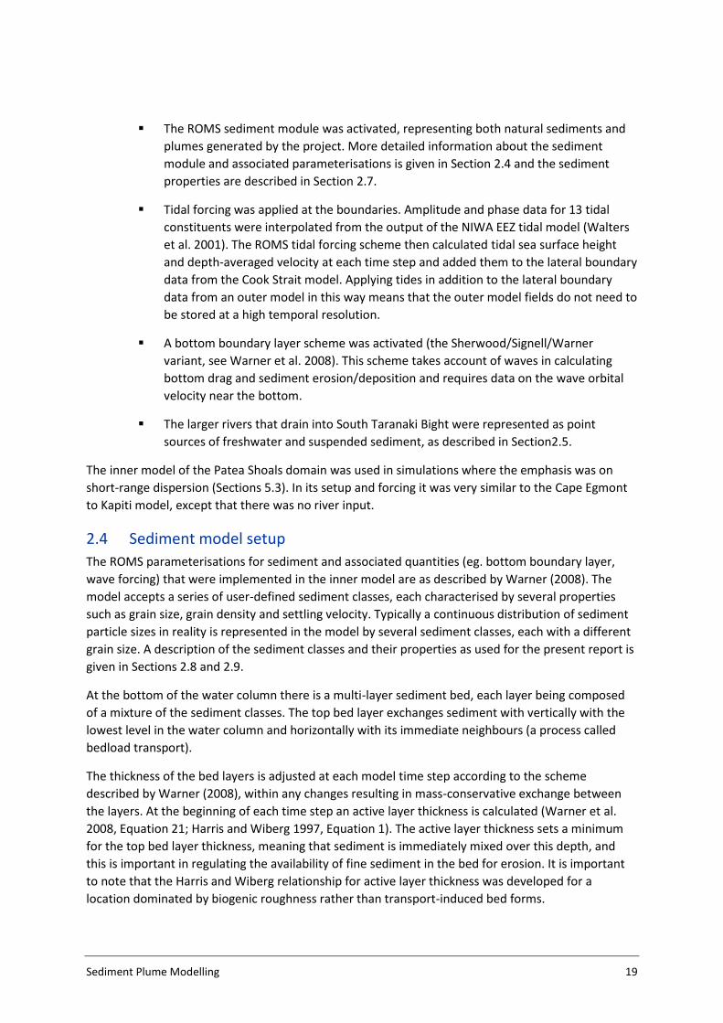
The ROMS sediment module was activated, representing both natural sediments and
plumes generated by the project. More detailed information about the sediment
module and associated parameterisations is given in Section 2.4 and the sediment
properties are described in Section 2.7.
Tidal forcing was applied at the boundaries. Amplitude and phase data for 13 tidal
constituents were interpolated from the output of the NIWA EEZ tidal model (Walters
et al. 2001). The ROMS tidal forcing scheme then calculated tidal sea surface height
and depth-averaged velocity at each time step and added them to the lateral boundary
data from the Cook Strait model. Applying tides in addition to the lateral boundary
data from an outer model in this way means that the outer model fields do not need to
be stored at a high temporal resolution.
A bottom boundary layer scheme was activated (the Sherwood/Signell/Warner
variant, see Warner et al. 2008). This scheme takes account of waves in calculating
bottom drag and sediment erosion/deposition and requires data on the wave orbital
velocity near the bottom.
The larger rivers that drain into South Taranaki Bight were represented as point
sources of freshwater and suspended sediment, as described in Section2.5.
The inner model of the Patea Shoals domain was used in simulations where the emphasis was on
short-range dispersion (Sections 5.3). In its setup and forcing it was very similar to the Cape Egmont
to Kapiti model, except that there was no river input.
2.4 Sediment model setup
The ROMS parameterisations for sediment and associated quantities (eg. bottom boundary layer,
wave forcing) that were implemented in the inner model are as described by Warner (2008). The
model accepts a series of user-defined sediment classes, each characterised by several properties
such as grain size, grain density and settling velocity. Typically a continuous distribution of sediment
particle sizes in reality is represented in the model by several sediment classes, each with a different
grain size. A description of the sediment classes and their properties as used for the present report is
given in Sections 2.8 and 2.9.
At the bottom of the water column there is a multi-layer sediment bed, each layer being composed
of a mixture of the sediment classes. The top bed layer exchanges sediment with vertically with the
lowest level in the water column and horizontally with its immediate neighbours (a process called
bedload transport).
The thickness of the bed layers is adjusted at each model time step according to the scheme
described by Warner (2008), within any changes resulting in mass-conservative exchange between
the layers. At the beginning of each time step an active layer thickness is calculated (Warner et al.
2008, Equation 21; Harris and Wiberg 1997, Equation 1). The active layer thickness sets a minimum
for the top bed layer thickness, meaning that sediment is immediately mixed over this depth, and
this is important in regulating the availability of fine sediment in the bed for erosion. It is important
to note that the Harris and Wiberg relationship for active layer thickness was developed for a
location dominated by biogenic roughness rather than transport-induced bed forms.

20 Sediment Plume Modelling
For the simulations described below the total sediment bed thickness was set initially to 1 m, with
eight layers. Initial layer thickness was 0.125 m, but this adjusts after the first time step. Incidentally,
the ROMS model optionally allows for the depth at the base of the water column to be adjusted as
the total sediment bed thickness changes, but this facility was turned off for the present simulations.
Vertical exchange of sediment between the top bed layer and the water column is the sum of two
terms (Warner 2008, Equation 22). The first is deposition: it occurs continuously and is calculated
separately for each sediment class as the product of the near-bottom concentration and the settling
velocity. The second is erosion (Warner 2008, Equation 23; Ariathurai and Arulanandan 1978): it
occurs only when the bottom stress exceeds a critical value, user-specified for each class.
Bedload transport (Warner et al. 2008 Section 3.4) is optionally calculated with the Soulsby and
Damgaard (2005) formulation. This process has been included in only one of the simulations
described below (the patch source simulation, Section 5.3) where it results in a modest increase,
around 20%, in the rate at which medium sands are transported out of the patch area, relative to a
simulation with bedload transport excluded.
Bottom stress is calculated with the Sherwood, Signell and Warner bottom boundary layer
formulation (Warner et al. 2008, Section 3.7). This requires data on the height, period and direction
of surface wind waves. Two sources were considered: the NZWAVE wave forecasting model5 and
dedicated runs of the SWAN wave model (R. Gorman, pers. comm). Another choice to be made in the
model setup was the bottom roughness formulation. A bottom roughness length is calculated from
the median grain density of the sediment bed (Warner et al. 2008, Equation 44). This changes as the
composition of the sediment bed evolves but for the simulations below it was typically ~0.4 mm.
Additional terms account for sediment bedload transport (Warner et al. 2008, Equation 45) and for
bedform ripples (Warner et al. 2008, Equation 46). The roughness length associated with bedload
transport was negligible in these simulations. The bedform roughness length varied in space and time
but was generally largest at around 20–30 m depth, where it was 0.5–2.5 mm. All these terms can be
enabled or disabled in the ROMS code. As part of the calibration process, several simulations were
carried out with different combinations of forcings and processes, the calibration target in this case
being measured SSC data (Section 4). The model configuration finally selected used NZWAVE wave
data and neglected the bedform roughness length. The main problem with the latter was that, when
it was included, the model was not able to reproduce the isolated spikes that are seen by the ABS in
near-bottom SSC (Section 4.3).
Figure 2-5 presents several time series relevant to erosion and deposition processes. The location is
in a water depth of 31 m depth on outer Patea Shoals and appears elsewhere in this report as mining
site A. It is characterised by strong tidal currents, moderately large wave amplitudes and complex
bedforms (Section 4.3 this report; MacDonald et al. 2012, Figure 3-56). It is one of 24 locations in the
model where hourly data have been saved to allow evaluation of short-timescale phenomena like
tides.
5 NZWAVE is part of the NIWA Ecoconnect environmental forecasting system: http://EcoConnect.niwa.co.nz/

Sediment Plume Modelling 21
a)
b)
c)
Figure 2-5: Bottom boundary layer & sediment bed time series at instrument site 7. a) Near-bottom current speed; b) bottom wave orbital speed; c) sediment bed active layer thickness.
Panel a shows the near-bottom current speed. Values are generally less than 0.4 m/s, with occasional
excursions as high as 0.75 m/s. Panel b shows the near-bottom wave orbital velocity, calculated
within ROMS from NZWAVE wane height and period data. The wave orbital velocity is frequently
higher than the current speed (note the different vertical scale) with several excursions above 1 m/s.
This indicates that waves will frequently be more effective in lifting sediment from the seabed than

22 Sediment Plume Modelling
currents. Panel c shows the active layer thickness calculated by ROMS. It is generally less than
10 mm, but occasionally exceeds 40 mm, with all the peaks coinciding with wave events. The figure
suggests that erosion of bottom sediments here (and in shallower water) tends to occur in occasional
high-wave events and that in the model these mix the upper sediment bed at this location to a depth
of at least 40 mm.
2.5 River inputs
Data for some 40 rivers were extracted from the NIWA Water Resources Explorer (WRENZ) website6
(Hicks et al. 2011) and 11 were selected for inclusion in the model based on their mean flow rate and
sediment input rate (Table 2-1). The rivers that were selected comprised the ten with the highest
flow rate, plus the Tangahoe River, which ranks 13th for flow but 9th for sediment input.
The model was supplied with a time series of daily-average flow rate and sediment input for each
river. The flow rate was estimated from gauging station data collected by NIWA, Taranaki Regional
Council and Horizons Regional Council. The gauging station data was available for all rivers except the
Tangahoe, for which the WRENZ mean flow was used throughout. Where the gauging station was
well upstream from the coast, the data were scaled by the ratio between the catchment area above
the gauging station and the total catchment area. For several rivers, data were not available after
Dec 2012; these gaps, plus a few short gaps elsewhere in the record, were filled with the WRENZ
mean flow.
Table 2-1: Rivers represented in the inner model, with mean freshwater and sediment input rates from WRENZ.
Name Flow rate (m3/s)
Sediment rate (kg/s)
Whanganui River 229.0 149.03
Manawatu River 129.5 118.46
Rangitikei River 76.4 35.04
Whangaehu River 47.2 21.82
Patea River 30.4 9.85
Waitotara River 23.3 15.08
Otaki River 30.1 5.46
Whenuakura River 9.9 8.75
Kaupokonui Stream 8.6 0.31
Turakina River 8.4 9.54
Tangahoe 4.2 1.39
Total 593 373
For the Whanganui River, a time series of SSC was available up to December 2012 from Horizons
Regional Council. A relationship between SSC and flow was established from the data before this
time (Figure 2-6) and used to fill the remainder of the SSC time series. (No filling of the flow time
series was required, as a complete flow dataset was available.)
6 http://wrenz.niwa.co.nz
Sediment Plume Modelling 23
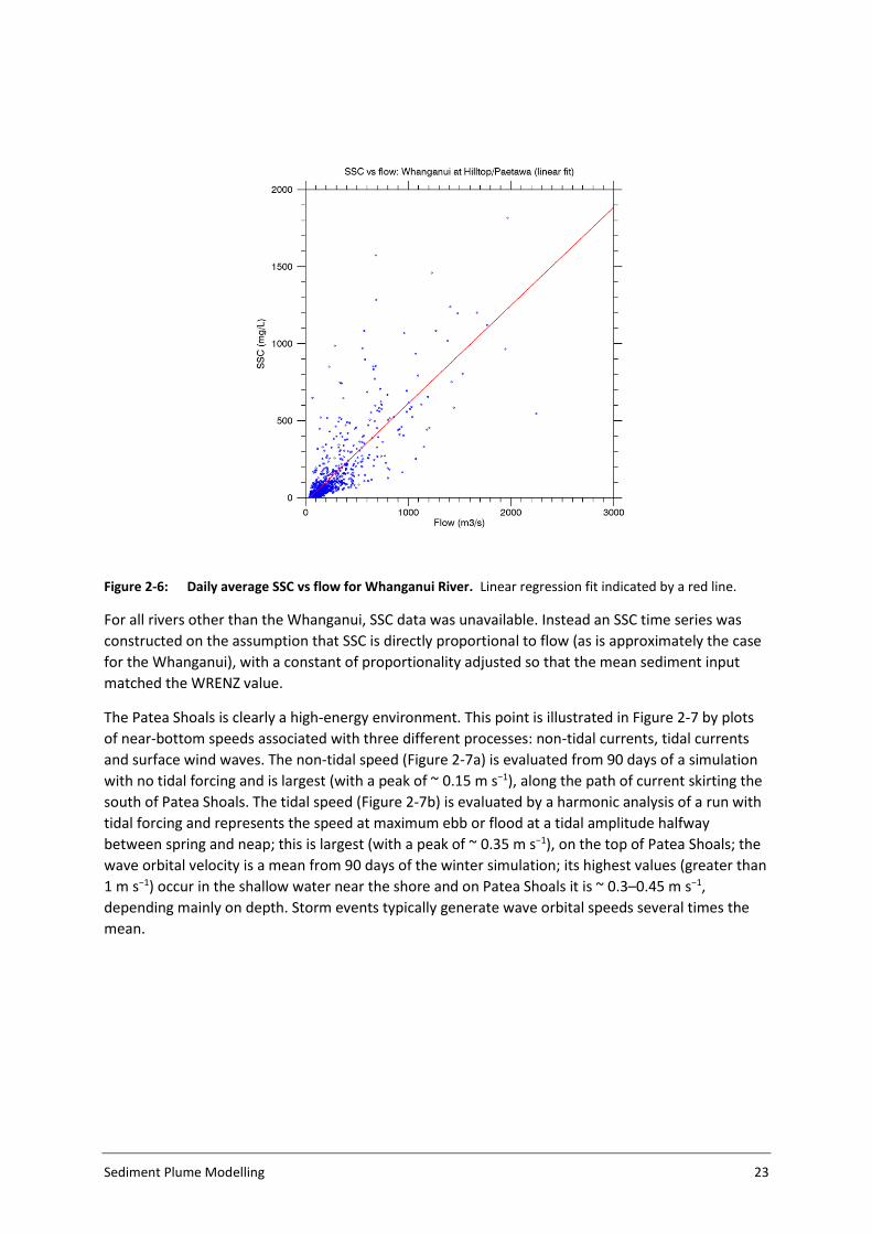
Figure 2-6: Daily average SSC vs flow for Whanganui River. Linear regression fit indicated by a red line.
For all rivers other than the Whanganui, SSC data was unavailable. Instead an SSC time series was
constructed on the assumption that SSC is directly proportional to flow (as is approximately the case
for the Whanganui), with a constant of proportionality adjusted so that the mean sediment input
matched the WRENZ value.
The Patea Shoals is clearly a high-energy environment. This point is illustrated in Figure 2-7 by plots
of near-bottom speeds associated with three different processes: non-tidal currents, tidal currents
and surface wind waves. The non-tidal speed (Figure 2-7a) is evaluated from 90 days of a simulation
with no tidal forcing and is largest (with a peak of ~ 0.15 m s−1), along the path of current skirting the
south of Patea Shoals. The tidal speed (Figure 2-7b) is evaluated by a harmonic analysis of a run with
tidal forcing and represents the speed at maximum ebb or flood at a tidal amplitude halfway
between spring and neap; this is largest (with a peak of ~ 0.35 m s−1), on the top of Patea Shoals; the
wave orbital velocity is a mean from 90 days of the winter simulation; its highest values (greater than
1 m s−1) occur in the shallow water near the shore and on Patea Shoals it is ~ 0.3–0.45 m s−1,
depending mainly on depth. Storm events typically generate wave orbital speeds several times the
mean.

24 Sediment Plume Modelling
Figure 2-7: Near-bottom speeds (m s−1) on the Cape Egmont to Kapiti inner model domain. (a) Mean non-tidal speed. (b) Maximum tidal speed (semi-major axis) of the main lunar semi-diurnal constituent, M2. (c) Mean bottom wave orbital speed.

Sediment Plume Modelling 25
2.6 Sediment model setup
Sediment calculations were carried out on the two inner domains (which were used for different
purposes), each nested within a larger-scale Greater Cook Strait model (Figure 2-1). Here we use
Greater Cook Strait to refer to the waters between the Tasman Sea (to the west) and the Pacific
Ocean (to the east). Cook Strait itself is shown in Figure 1-1, being the narrowest stretch of water
between the North and South Islands of New Zealand.
2.7 Sediment properties and release parameters
The sediment scheme in the ROMS modelling system requires the modeller to define a set of
sediment classes and, for each one, to specify several properties, notably: median grain size; grain
density; porosity (when in the sediment bed); settling velocity (when in suspension); critical bed
shear stress for erosion and deposition; and a rate parameter used in the formula relating erosion
rate to bed shear stress. The number of sediment classes is unlimited, but the computational
expense increases for each additional class.
The results presented in this report were produced with the ROMS sediment model on one of the
inner domains. The following sub-sections describe the different sediment classes
2.8 Background sediments
The base simulation represents background sediment processes using 7 sediment classes:
The river-derived sediments that are injected by the rivers. There are two classes: a
coarse silt (16–63 µm) and a fine silt/clay (< 16 µm).
The seabed-derived sediments comprise the seabed at the beginning of the simulation.
They range from a coarse sand (500–1000 µm) to a fine silt (4–16 µm).
There were two reasons for introducing the background sediments:
Primarily, to support a realistic interaction between the mining-derived sediment
plumes and the seabed;
Secondarily, to produce estimates of background suspended sediment concentrations
that are approximately correct and can be compared with predictions of sediment
concentrations resulting from the ironsand extraction operation.
The seabed is initially populated with a combination of coarse sand (500–1000 µm, 20%), fine–
medium sand (128–500 µm, 72%), very fine sand (63–128 µm, 6%), coarse silt (16–63 µm, 1.5%) and
fine silt (4–16 µm, 0.5%). The proportions were initially based on seabed particle size distribution
(PSD) data from the extraction area, and the fine sediment fractions were then adjusted so that the
model produces surface SSCs of approximately the correct magnitude in the near-shore area
(Sections 4.2 and 4.1). The seabed composition was assumed to be uniform over the model domain.
For the present calculations, the background sediment parameters differed from those used in the
March 2014 calculation in two ways:
The minimum critical stress was increased from 0.1 to 0.2 Pa. in line with the HR
Wallingford findings.

26 Sediment Plume Modelling
We abandoned the imposition of a minimum settling velocity of 0.1 mm/s to
accurately represent flocculation for background sediments. While the process of
flocculation does tend to increase the settling velocity of the bulk of fine sediments,
the laboratory results suggest that it leaves a residual level of very slow-settling
material. Therefore the minimum settling velocity for both riverine and seabed
background sediments was reduced from 0.1 mm/s to 0.01 mm/s.
The background sediment parameters are listed in Table 2-2, with changes from the March 2014
configuration highlighted in a bold font. Other properties required by ROMS include an erosion rate
parameter (2 × 10⁻⁴ kg m−2 s−1 for all classes) and a porosity (0.4 for all classes).
Table 2-2: Background sediment parameters. Values that differ from the March 2014 configuration are shown in a bold font.
Label Source Nominal size range
(µm)
Settling velocity (mm/s)
Critical stress (Pa)
Fraction initially present
in seabed
sand_01 River 16–63 0.63 0.200
sand_02 River 4–16 0.01 0.200
sand_03 Seabed 500–1000 103 0.431 20%
sand_04 Seabed 128–500 38 0.219 72%
sand_05 Seabed 63–128 6.3 0.200 6%
sand_06 Seabed 16–63 0.76 0.200 1.5%
sand_07 Seabed 4–16 0.01 0.200 0.5%
Note that we also considered using a non-zero external concentration (~0.1–0.5 mg/L) for the finest
seabed class (sand_07) to provide an input of fine sediment from outside the model domain. This
was intended to offset the tendency of the model to underestimate the mean SSC south of Patea
Shoals in comparison with remote sensed data (Section 4.2). After subsequent discussions with Dr
Matt Pinkerton it was decided to represent this material by an adjustment in the optical post-
processing of the model output (Pinkerton 2015c) and the external concentration was set to zero.
The model of background sediment processes was initialised at 2000 days (relative to a reference
time of 00:00 UTC on 1 January 2005) and run to 3000 days, with statistical analyses based on the
last 730 days of the simulation. The sediment bed adjusts within the first 100–200 days after
initialisation as the finer classes are stripped out of the uppermost bed layer in high-energy areas like
Patea Shoals but remain in low-energy areas. A slower adjustment process occurs throughout the
duration of the simulation as seabed material continues to be eroded from the high-energy areas
and deposited in the low-energy areas.
2.9 Mining-derived sediments
Two main sediment streams from the ironsand extraction are considered: the hydro-cyclone
overflow discharge and the de-ored sand discharge. The hydro-cyclone overflow results from
dewatering of the de-ored sand before it is pumped to the bottom. It is a discharge of mostly fine
sediment with a large flow (8.8 m3/s) of water. The de-ored sand discharge involves de-watered, de-
ored sand being released from a pipe with a view to depositing it as compactly as possible, usually
into a pit that has been excavated earlier. The de-ored sand is predominantly fine–medium sand
(125–500 µm) with some finer material. Both discharges are no more than 4 m or so above the

Sediment Plume Modelling 27
bottom and in the current proposal are released close to each other, with a view to maximising the
trapping of fine sediment in the pit with the coarser sands.
These combined sediment stream is represented in the model by two different mechanisms, treated
in different simulations. The first, the suspended source, is a continuous source of fine suspended
sediment. The second, the patch source, is a 3 × 2 km rectangular patch of sand representing the
area filled by one year’s mining and containing all the material that has not been released in the
suspended source. The set-up of the simulations that implement these two sources is described
further below.
2.9.1 Suspended source
The suspended-source sediment parameters in the current simulations are based on laboratory and
model results outlined in the HRW report (HRW 2015). The resulting classification is presented in
Table 2-3.
Table 2-3: Suspended source sediment parameters. The discharge rate is for a plant throughput of 50 Mt/a. Values that differ from the March 2014 configuration are shown in a bold font.
The movement from a grain-size-based classification (March 2014) to a settling-velocity-based
classification has not changed the settling velocity of the finest sediment classes, which remain at
0.1 mm/s and 0.01 mm/s. These are the sediment types that are most readily mixed to the surface
and they are the most optically active, so they are the sediment types that are most important in
determining the near-surface SSC and optical effects. The changes in the discharge rates for these
sediment classes are summarised in Table 2-4.
Table 2-4: Summary of changes in discharge rates for the finer mining-derived sediments. .
Another difference from the March 2014 simulations is the depth at which the tailings discharge is
introduced into the model. For the March 2014 simulations this release height was assumed to be

28 Sediment Plume Modelling
15 m below the surface, based on the plant design information that was available when the
simulations were originally set up (in June/July 2013). Since then it has become clear that:
The discharge point for the tailings will be lower than originally indicated, nominally
about 4–6 m above the bottom.
Subsequent to the discharge the plume will descend to the bottom and form a bottom-
attached plume of a few metres thickness (Hadfield 2014c).
2.9.2 Patch source
Of the fine sediments (< 63 μm) that are released with the tailings, a fraction will settle to the bottom
in the mining pit and then be buried with the de-ored sand. This fraction, which depends strongly on
settling velocity, was quantified by HR Wallingford (2015) and taken into account in setting the
suspended source discharge rates (Section 2.9.1). The trapped fine sediment is then available for
resuspension at a rate controlled by the erosion of the sand and the concentration of the fine
sediment in the sand matrix.
To model this process we consider a rectangular patch representing one year’s worth of ironsand
extraction and populate this patch with material that reflects the composition of the combined
hydro-cyclone and de-ored sand discharge streams, minus all the material that was released in the
suspended source.
The area of this source is calculated as follows: Assuming a volume extraction rate of 1.195 m3/s at
full operation (mass extraction rate 8000 tonne/h with a bulk density of 1860 kg/m3) and an up-time
of 80%, the annual volume extracted is 30.15 × 10⁶ m3. At a mean mined depth of 5 m, this indicates
that an area of 6.05 km2 would be mined in one year. This area is represented in the model as a
3 × 2 km rectangular patch centred on the mining site, which is taken to be mining site A.
The patch source was implemented in the inner model on the Patea Shoals domain. The sediment
model included the five seabed sediment classes, but not the riverine sediment classes (as the major
rivers are outside this domain and are not important for the predominantly short-range, near-bottom
transport involved). In addition there were three “patch” sediment classes representing the trapped
fine sediment. The model was initialised at 2000 days with seabed sediments filling the domain, then
at 2200 days the seabed in the 3 × 2 km patch area was repopulated with a mixture of the three
coarsest seabed sediment classes and the three patch classes. The simulation was continued to
3000 days.
The composition to which the patch was set at 2200 days (Table 2-5) was calculated from the same
discharge rate data for fine sediments (including flocculated fine sediments) as was used in deriving
the suspended source parameters (Table 2-3) but this time considering the fraction trapped on the
bottom rather than the fraction remaining in suspension. The total rate at which fine sediment is
discharged and trapped in the pit is 71 kg/s and this material mixes with the de-ored sand, which is
discharged at 1910 kg/s. The trapped fine sediment (classes sand_06 to sand_08) therefore
comprises 3.7% of the patch. For simplicity, the remainder of the patch is assumed to be composed
of the three coarsest classes in the original seabed, with the proportions adjusted slightly to ensure
the total is 100%.

Sediment Plume Modelling 29
Table 2-5: Patch sediment parameters. The initial mass fraction column specifies the seabed composition at the start of the simulation. The patch mass fraction column specifies the seabed composition imposed inside the 3 × 2 km patch at 2200 days.
30 Sediment Plume Modelling
3 Hydrodynamic model evaluation
3.1 Field measurements
A programme of field measurements was carried out in the area from Patea Shoals to Whanganui,
involving instrument deployments at several sites for three periods between September 2011 and
July 2012. The programme is described in detail in a dedicated report (MacDonald et al. 2012). The
data that are most relevant for the sediment plume modelling are:
Vertical velocity profiles from acoustic Doppler current profilers (ADCPs) at five sites,
shown in Figure 2-1b.
Profiles of temperature and salinity from moored sensors at several sites.
Measurements of suspended sediment from optical and acoustic backscatter sensors
(OBS and ABS).
Below, in the present section, modelled velocities are compared with the ADCP measurements. In
Section 4 modelled near-bottom suspended sediment (sand) concentrations are compared with ABS
data to give an approximate check on the model’s representation of bed resuspension processes.
The times and locations at which ADCP data are available are listed in Table 3-1.
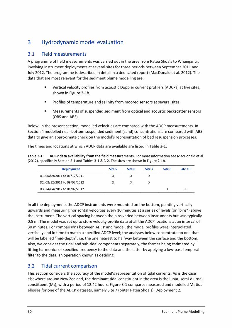
Table 3-1: ADCP data availability from the field measurements. For more information see MacDonald et al. (2012), specifically Section 3.1 and Tables 3-1 & 3-2. The sites are shown in Figure 2-1b.
Deployment Site 5 Site 6 Site 7 Site 8 Site 10
D1, 06/09/2011 to 01/12/2011 X X X
D2, 08/12/2011 to 09/02/2012 X X X
D3, 24/04/2012 to 01/07/2012 X X
In all the deployments the ADCP instruments were mounted on the bottom, pointing vertically
upwards and measuring horizontal velocities every 10 minutes at a series of levels (or “bins”) above
the instrument. The vertical spacing between the bins varied between instruments but was typically
0.5 m. The model was set up to store velocity profile data at all the ADCP locations at an interval of
30 minutes. For comparisons between ADCP and model, the model profiles were interpolated
vertically and in time to match a specified ADCP level; the analyses below concentrate on one that
will be labelled “mid-depth”, i.e. the one nearest to halfway between the surface and the bottom.
Also, we consider the tidal and sub-tidal components separately, the former being estimated by
fitting harmonics of specified frequency to the data and the latter by applying a low-pass temporal
filter to the data, an operation known as detiding.
3.2 Tidal current comparison
This section considers the accuracy of the model’s representation of tidal currents. As is the case
elsewhere around New Zealand, the dominant tidal constituent in the area is the lunar, semi-diurnal
constituent (M2), with a period of 12.42 hours. Figure 3-1 compares measured and modelled M2 tidal
ellipses for one of the ADCP datasets, namely Site 7 (outer Patea Shoals), Deployment 2.
Sediment Plume Modelling 31
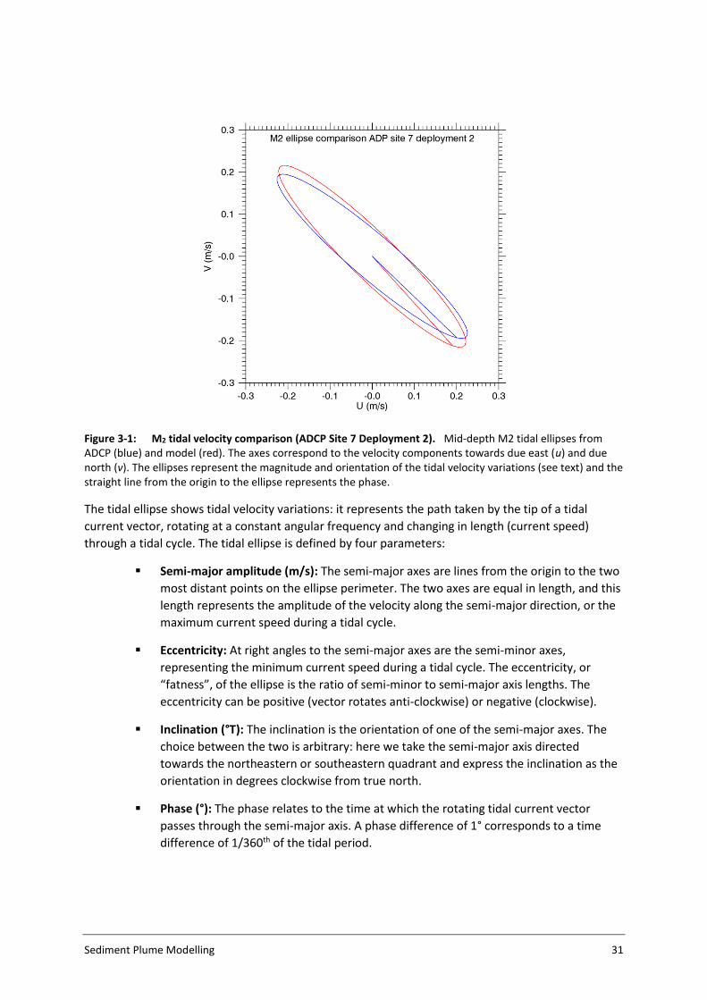
Figure 3-1: M2 tidal velocity comparison (ADCP Site 7 Deployment 2). Mid-depth M2 tidal ellipses from ADCP (blue) and model (red). The axes correspond to the velocity components towards due east (u) and due north (v). The ellipses represent the magnitude and orientation of the tidal velocity variations (see text) and the straight line from the origin to the ellipse represents the phase.
The tidal ellipse shows tidal velocity variations: it represents the path taken by the tip of a tidal
current vector, rotating at a constant angular frequency and changing in length (current speed)
through a tidal cycle. The tidal ellipse is defined by four parameters:
Semi-major amplitude (m/s): The semi-major axes are lines from the origin to the two
most distant points on the ellipse perimeter. The two axes are equal in length, and this
length represents the amplitude of the velocity along the semi-major direction, or the
maximum current speed during a tidal cycle.
Eccentricity: At right angles to the semi-major axes are the semi-minor axes,
representing the minimum current speed during a tidal cycle. The eccentricity, or
“fatness”, of the ellipse is the ratio of semi-minor to semi-major axis lengths. The
eccentricity can be positive (vector rotates anti-clockwise) or negative (clockwise).
Inclination (°T): The inclination is the orientation of one of the semi-major axes. The
choice between the two is arbitrary: here we take the semi-major axis directed
towards the northeastern or southeastern quadrant and express the inclination as the
orientation in degrees clockwise from true north.
Phase (°): The phase relates to the time at which the rotating tidal current vector
passes through the semi-major axis. A phase difference of 1° corresponds to a time
difference of 1/360th of the tidal period.

32 Sediment Plume Modelling
The tidal ellipses shown in Figure 3-1 clearly match reasonably well in magnitude and orientation.
Similar ellipses for the other ADCP deployments are shown in Appendix B, Figure B-1. Overall
agreement is very good. The semi-major amplitudes agree to within ±6%; the eccentricities agree
within ±0.04, the inclinations within ±8°, and the phases within ±2.4° (5.0 minutes). This is a very
good match.
The tidal current amplitude normally decreases towards the bottom due to friction. Figure 3-2
compares measured and modelled vertical profiles of the M2 semi-major amplitude for the same
ADCP dataset as Figure 3-1. The agreement in the middle and upper water column is very good (as
was evident from Figure 3-1). Measured and modelled amplitudes both decrease towards the
bottom, as expected. The lowest level at which data are available from the ADCP instrument at this
site is 2.05 m above the bottom: here the modelled amplitude exceeds the measured amplitude by
10%. Similar profiles for the other ADCP deployments are shown in Figure B-2. Agreement is
generally good, with a tendency for modelled amplitude to exceed measured amplitude by a modest
amount in the lowest few metres. This may indicate that the effective bottom roughness is
somewhat lower in the model than in reality.
Figure 3-2: M2 tidal current profile comparison (ADCP Site 7 Deployment 2). Semi-major amplitude of the M2 tide versus height above the bottom from ADCP (blue) and model (red).
The M2 constituent dominates the tidal velocity but several smaller-amplitude constituents also
contribute. The larger ones in this area are S2 (12 hours), N2 (12.66 hours), and K1 (23.93 hours), for
which mid-depth tidal ellipses are compared in Figure 3-3. Note the different velocity scale in this
figure relative to Figure 3-1. Agreement is good, though not as close as for M2. The largest mismatch
evident in these graphs is a difference of 31°, or 2.1 hours, in the phase of the K1 constituent. This
difference probably results from a bias in the lateral boundary data taken from the EEZ tidal model,
which is known to have significant errors for this constituent in this region (Stanton et al. 2001).

Sediment Plume Modelling 33
Figure 3-3: Tidal velocity comparison for S2, N2 and K1 (ADCP Site 7 Deployment 2). Mid-depth tidal ellipses from ADCP (blue) and model (red).
3.3 Sub-tidal current comparison
A comparison of sub-tidal currents is shown in Figure 3-4. The upper panel in this figure shows a
scatter plot of velocities, with the ellipse in this case being a variance ellipse, a conventional
representation of the magnitudes of variability in velocity data. A variance ellipse can be
characterised by its semi-major axis (in this context called a principal axis), eccentricity and
inclination, like a tidal ellipse. However a variance ellipse does not have a phase (since it says nothing
about the timing of the variability) and its eccentricity has no sign (since it says nothing about the
rotation of velocity vectors). Also, the centres of the variance ellipses in Figure 3-4 are offset from
the origin by an amount representing the mean current over the period of the deployment. The
lower two panels in the figure indicate how well the fluctuations in sub-tidal velocity match up in
time. The centre panel shows fluctuations along the principal axis of maximum variability (this being
a compromise between the principal axes of the observed and modelled variance ellipses) and the
bottom panel shows fluctuations perpendicular to this axis.

34 Sediment Plume Modelling
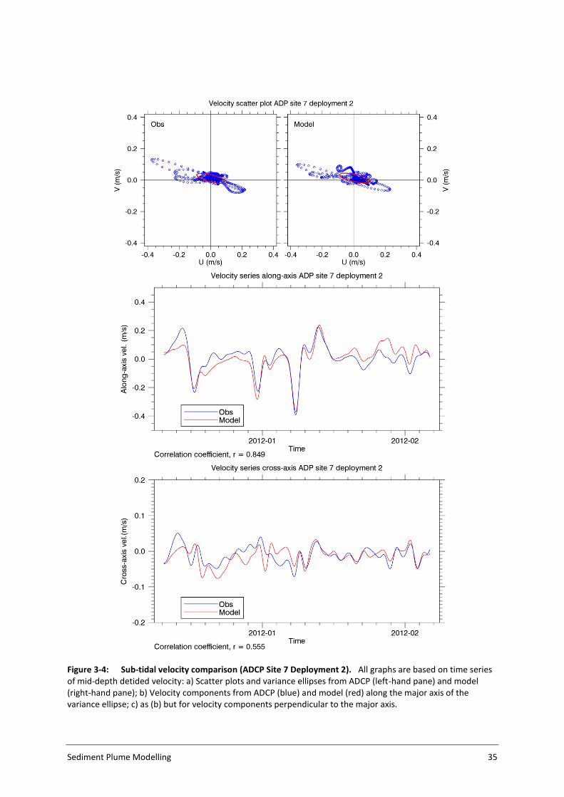
Figure 3-4 indicates good agreement between model and measurements for the ADCP deployment in
question. The variance ellipses have a similar shape and orientation, there is a high correlation (r =
0.849) between measured and modelled fluctuations along the principal axis and a somewhat lower
correlation (r = 0.555) perpendicular to this. The mean current (the offset of the centre of the ellipse)
is small relative to the dimensions of the ellipse but appears to be directed to the east in both cases.
On a technical matter, the time series in Figure 3-4 are quite smooth, as a result of the application of
a low-pass filter in detiding the data. (The filter is the 51G113 filter from Thompson, 1983, applied to
hourly values; see Figure 2 of that article for the filter’s frequency response.) To investigate the effect
of this smoothing, the model-measurement comparison has been repeated with an alternative
method, namely, removal of the tides by analysing a set of several tidal constituents (3 semi-diurnal
and 2 diurnal) from the data and then constructing and subtracting the tidal time series. A
comparison of the results of the two methods (Figure 3-5, along with other output not shown)
indicates that the latter method of detiding does leave more high-frequency information in the data,
but for the purposes of comparison between model and measurements, both methods give similar
results, as long as the model and measurement time series are detided in the same way.
Sediment Plume Modelling 35
Figure 3-4: Sub-tidal velocity comparison (ADCP Site 7 Deployment 2). All graphs are based on time series of mid-depth detided velocity: a) Scatter plots and variance ellipses from ADCP (left-hand pane) and model (right-hand pane); b) Velocity components from ADCP (blue) and model (red) along the major axis of the variance ellipse; c) as (b) but for velocity components perpendicular to the major axis.

36 Sediment Plume Modelling
Figure 3-5: Comparison of detiding methods (ADCP Site 7 Deployment 2). The along-axis time series comparison of Figure 3-4 detided with the 51G113 low-pass filter (upper panel) and tidal analysis and removal (lower panel).
A comprehensive set of comparisons for the mid-depth sub-tidal currents is presented in Appendix B.
Variance ellipses are compared in Figure B-3, along-axis time series in Figure B-4 and across-axis time
series in Figure B-5; the numeric values are tabulated in Table B-2. In assessing the degree of
agreement between the measured and modelled mean currents, one should remember that in
several cases the mean currents are small relative to the variability. Both measurements and model
indicate a mean flow directed towards east-southeast (90–110°) at all locations except Site 7, where
the mean current is directed to the northeast (35–75°). Modelled and measured directions agree to
within ±10°, with a couple of exceptions where the magnitude of the mean measured current is very
small. Modelled and measured magnitudes agree to within ±0.03 m/s, with the exception of Site 8
Deployment 3, where the modelled magnitude (0.09 m/s) is 1.5 times the measured magnitude
(0.06 m/s). Comparing measured and modelled values of semi-major axis length, the model under-
predicts this quantity by ~35% at the Site 5, ~30% at Site 6, and 0–12% at the other sites. The
eccentricity and inclination of the variance ellipse are very close for all deployments (eccentricity
within ±0.09, inclination within ±7°). When a comparison is made between measured and modelled
velocity components, along and across the principal axis, the correlation is high for the along-axis
components in all cases (r = 0.85–0.93) and lower for the across-axis component. For Site 5 the cross-
axis correlations are small, however the low eccentricity of the variance ellipses at this site implies
Sediment Plume Modelling 37
that the across-axis currents are very weak; at the other sites the cross-axis correlations are larger
(r = 0.55–0.84).
The same set of comparisons has been done for sub-tidal currents 5 m below the surface and at the
lowest ADCP level. Near the surface Table B-3, the overall pattern of the comparison is similar to the
mid-depth comparison. The currents (in terms of mean magnitude and semi-major amplitude) are
generally somewhat stronger near the surface and temporal correlations slightly higher. The ratio
between modelled and measured semi-major amplitude is higher, and is now around 1.1 at the outer
sites (7–10). Near the bottom (Table B-4) the same differences are seen in reverse. Compared to the
mid-depth, currents are somewhat weaker, temporal correlations slightly lower, and the model
tends to under-predict the semi-major amplitude a little more. For two datasets (Site 6, Deployment
2 and Site 7, Deployment 2) the modelled and measured mean directions differ greatly by 169° and
84°, respectively, but in both cases the mean current (0.01 m/s) is small relative to the variability
(semi-major amplitude 0.05–0.08 m/s).
The degree of agreement here between the modelled and the measured velocities is as good as, or
better than, that achieved in other modelling exercises on the New Zealand continental shelf (e.g.
Hadfield and Zeldis 2012). The major reservation relates to the wind-driven variability: a relatively
large factor (1.4) has been applied to the wind stresses, and with this factor the model
underestimates the variability (semi-major axis amplitude) at the sites closest to the coast (Sites 5
and 6). The most likely explanation is that the surface wind data from the NZLAM atmospheric model
do not fully capture the channelling and acceleration of winds through Greater Cook Strait. However
confirmation of this explanation would require data from a higher-resolution atmospheric model.
The implications of the model underestimating the wind-driven variability near the coast on
sediment transport are not entirely clear, but it is likely that the model will underestimate the extent
to which river plumes will be spread along the coast.
38 Sediment Plume Modelling
4 Sediment model evaluation
4.1 Surface SSC comparison with in situ measurements
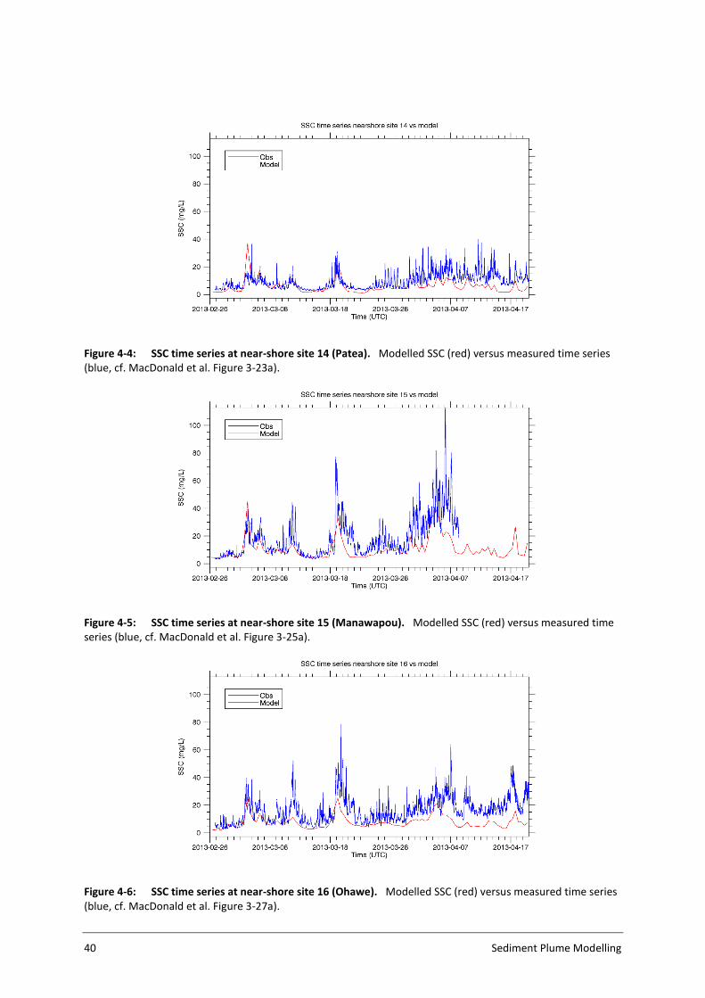
Comparisons between the observed SSC data and modelled SSC at the same locations and times
(Figure 4-1 to Figure 4-6) typically show a good correspondence between the two datasets in terms
of the timing of the peaks in SSC. Note that the observed data often show a strong tidal variation, but
these are not represented by the model output which is based on 12-hour averages. There is a
tendency evident for the model to underestimate SSC by a factor of up to two. For a highly variable
quantity like SSC this represents good agreement. The exception is at site 11 (Figure 4-1) which is
6 km east of the Whanganui River mouth. Here the model does not reproduce the observed increase
in SSC after 17 April: the measured SSC increases to around 50 mg/L whereas the modelled SSC
remains at 5 mg/L. Whanganui River flow data around this time indicate an increase in flow on 16
April. Animations of model SSC show the model produces a river plume with surface SSC of 20 mg/L,
but this does not extend to the measurement site. So the performance of the background SSC model
in high Whanganui River flow conditions remains unverified close to the river mouth.

Sediment Plume Modelling 39
Figure 4-1: SSC time series at near-shore site 11 (Whanganui). Modelled SSC (red) versus measured time series.
Figure 4-2: SSC time series at near-shore site 12 (Kai Iwi). Modelled SSC (red) versus measured time series (blue, cf. MacDonald et al. Figure 3-19a).
Figure 4-3: SSC time series at near-shore site 13 (Waitotara River). Modelled SSC (red) versus measured time series (blue, cf. MacDonald et al. Figure 3-21a).
40 Sediment Plume Modelling
Figure 4-4: SSC time series at near-shore site 14 (Patea). Modelled SSC (red) versus measured time series (blue, cf. MacDonald et al. Figure 3-23a).
Figure 4-5: SSC time series at near-shore site 15 (Manawapou). Modelled SSC (red) versus measured time series (blue, cf. MacDonald et al. Figure 3-25a).
Figure 4-6: SSC time series at near-shore site 16 (Ohawe). Modelled SSC (red) versus measured time series (blue, cf. MacDonald et al. Figure 3-27a).

Sediment Plume Modelling 41
4.2 Surface SSC comparison with remote-sensed data
Remote sensing provides a basis for evaluating the background sediments. Three figures below
compare statistics of modelled near-surface, background SSC with a remote-sensed product called
total suspended solids (TSS), which was derived from satellite estimates of backscatter at 488 nm.
Backscatter was derived from the NASA ocean colour satellite sensor, MODIS-Aqua, using
measurements between 2002 and 2008. Data were processed using the Quasi-Analytical Algorithm
with local modification for the SMD derived from in situ bio-optical measurements (Pinkerton & Gall
2015). TSS includes the inorganic suspended sediment modelled here, but also phytoplankton and
suspended organic matter. Offshore, TSS is expected to exceed SSC, but near the shore the two
quantities should be approximately equal as inorganic sediment dominates.
Figure 4-7 shows a comparison for the 5th percentile (i.e. the value which exceeds 5% of the
measured or modelled data) evaluated at each grid point. The colour scale runs from 0.1 mg/L
(below which is shaded white) to 1000 mg/L (above which is shaded yellow). The same colour scale
with the same data range is used for all plots of SSC in this report. Figure 4-8 shows the 50th
percentile, or median, and Figure 4-9 the 95th percentile. In all cases there is a band of elevated
concentrations near the coast in both the model and remote-sensed estimates. The width of this
band is of the order of 5–20 km—depending on the particular percentile and the definition of
“elevated”—and the band tends to be widest over the relatively shallow water of the Patea Shoals.
At the coast between Hawera and Whanganui the modelled and remote-sensed concentrations
agree reasonably well. Approximate values are:
5th percentile: modelled = 2 mg/L and remote-sensed ~ 2 mg/L (but highly variable);
50th percentile: modelled = 10–15 mg/L and remote-sensed = 10–20 mg/L;
95th percentile: modelled = 40–60 mg/L, but > 100 mg/L at Whanganui River mouth
and remote-sensed = 40–60 mg/L.
In the region near the bottom of the figures and well outside the 22.2 km territorial limit,
approximate values are:
5th percentile: modelled < 0.001 mg/L and remote-sensed ~ 0.1 mg/L;
50th percentile: modelled ~ 0.001 mg/L and remote-sensed = 0.2–0.5 mg/L;
95th percentile: modelled ~ 0.01 mg/L and remote-sensed ~ 1 mg/L.
In other words, modelled SSC offshore is much lower than remote-sensed TSS. There are two likely
reasons for this:
As noted above, TSS includes organic components that are not included in the
modelled SSC;
Satellite images show that visible sediment plumes often extend from the southern
side of Greater Cook Strait, apparently associated with sediment input from the South
Island coast and rivers. However, the SMD receives no input of sediment from outside
its domain.

42 Sediment Plume Modelling
At the shoreward side of the Project Area, values are:
5th percentile: modelled = 0.01 mg/L and remote-sensed ~ 0.1 mg/L;
50th percentile: modelled = 0.3–0.4 mg/L and remote-sensed = 0.5 mg/L;
95th percentile: modelled 3 mg/L and remote-sensed ~ 3 mg/L.
So agreement is good, for the upper percentiles at least. At the seaward side of the proposed mining
area and further offshore, modelled concentrations are lower than the remote sensing estimate.
In the zone between the coast and the 22.2 km territorial limit, the modelled concentration contours
are generally further from the coast then the remote-sensed contours. This is particularly true over
Patea Shoals. In this region the comparison indicates that the model SSC overestimates remote-
sensed TSS by a factor in the vicinity of around two.
a)
b)
Figure 4-7: Modelled and observed 5th percentile surface concentration of background sediment. a) Model background SSC; b) remote-sensed TSS. Black lines indicate the project area and the 22.2 km territorial limit.
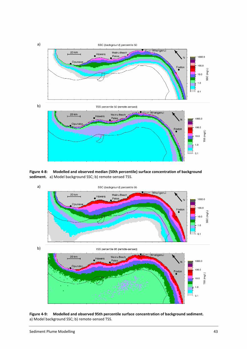
Sediment Plume Modelling 43
a)
b)
Figure 4-8: Modelled and observed median (50th percentile) surface concentration of background sediment. a) Model background SSC; b) remote-sensed TSS.
a)
b)
Figure 4-9: Modelled and observed 95th percentile surface concentration of background sediment. a) Model background SSC; b) remote-sensed TSS.

44 Sediment Plume Modelling
4.3 Near-bottom SSC comparison with in situ ABS data
This section presents a comparison of modelled near-bottom sand (> 63 µm) concentrations with
ABS data from instrument sites 6, 7, 8 and 10 on Patea Shoals (Figure 4-10 to Figure 4-13). In the
Oceanographic Measurements report the ABS data are presented in terms of a quantity called Cref,
the concentration at a reference level (MacDonald et al. 2012, Figures 3-45, 3-55, 3-57 and 3-58). For
comparison with the model they were converted to average concentrations over the lowest 1 m of
the water column (Iain MacDonald, pers. comm.), which more closely matches what the model
calculates.
The model produces a series of discrete resuspension events, which matches what the ABS observes.
However the model does not reproduce the large difference in observed SSC between site 7 (where
observed SSC reaches 500 mg/L on occasion and is generally under-predicted by the model), site 6
(where observed SSC exceeds 100 mg/L on only one occasion and is generally over-predicted by the
model) and the deeper sites, 8 and 10, where observed SSC is less than 20 mg/L and is over-predicted
by the model). The modelled near-bottom sand concentration generally peaks at around 100 mg/L at
the shallow sites and 60–80 mg/L at the deeper sites.
The large difference in sand concentration measured by the ABS between the shallower sites, 6 and
7, was noted by MacDonald et al. (2012) and attributed to the complex bedforms around Site 7 (their
Figure 3-56). They quote Green and Black (1999) who show that, given the same wave forcing,
differences in bed form geometry can give rise to concentration differences of a factor of 20.
Meanwhile at the deeper sites, biostabilisation by polychaete tube worms may be an important
factor stabilising the bed (Beaumont et al. 2013).
Our conclusion from the comparison is that the sediment model does not reproduce the wide range
of variation in susceptibility to sand resuspension between different locations on Patea Shoals, and
furthermore could not do so without a lot of tuning to local conditions. The formulation of
resuspension is likely to overestimate resuspension in some places and underestimate it in others.

Sediment Plume Modelling 45
Figure 4-10: Time series of near-bottom sand concentration at instrument site 6. Modelled sand concentration (red) versus estimate from ABS measurements.
Figure 4-11: Time series of near-bottom sand concentration at instrument site 7. Modelled sand concentration (red) versus estimate from ABS measurements.
Figure 4-12: Time series of near-bottom sand concentration at instrument site 8. Modelled sand concentration (red) versus estimate from ABS measurements.

46 Sediment Plume Modelling
Figure 4-13: Time series of near-bottom sand concentration at instrument site 10. Modelled sand concentration (red) versus estimate from ABS measurements.

Sediment Plume Modelling 47
5 Sediment model results This section presents results from the present sediment model configuration. In Appendix C, these
results are compared with results from the March 2014 configuration of the model, as presented to
the Decision Making Committee for the previous application.
5.1 Suspended source at mining location A
5.1.1 Selected cases
From the model output we prepared animations of the surface SSC plume generated by the
suspended source at mining location A. These animations show a rather mobile plume that clearly
responds to wind-driven fluctuations in the currents. In its most common configuration the plume
extends east-southeast from the source location. The present section shows 6 examples (Figure 5-1
to Figure 5-7) of the surface plume, along with vertical transects through the plume at various
locations. Each example occurred under different atmospheric forcing and the resultant plume varies
between case studies.
Winds for the region exhibit a tri-modal distribution where winds from the north, southeast and west
are the dominant modes. The cases-shown here are chosen primarily to reflect this. Case 1 occurs
near the beginning of the mining release of sediments and shows an early evolution of the plume.
Case 2 is chosen to provide an example of the plume under westerly winds. Case 3 is chosen as an
example when wind and wave forcing were minimal. Case 4 is chosen as it has northerly wind
forcing. Case 5 is chosen as it has southeasterly wind forcing. Case 6 is chosen because the plume
exhibited different behaviour to Case 5, even though wind forcing is similar.
Figure 5-1 and Figure 5-2 (Case 1) show the evolution of the plume near the initiation of mining. The
ocean currents in this region over this period tend to carry the mining plume towards the shore
before directing it along the coastline. In the vertical this plume becomes mixed throughout the
water column.
Figure 5-3 shows the SSC for Case 2. Here the winds were to be westerly for the 2 days leading up to
the image shown, and the wave amplitude was relatively large over this period. The resultant plume
is well mixed throughout the water column and stretches some way to the east and out along the
coastline.
Figure 5-4 shows the SSC for Case 3. The winds are weak and tend to be unidirectional, and the wave
forcing is also weak. In this scenario the plume stays near the mining site and sediment
concentrations are higher than in cases 1 and 2 (slightly under 10 mg/L as opposed to less than
5 mg/l).
Figure 5-5 shows the SSC for Case 4. In the 2 days prior the wind was northerly and the wave height
moderate. The plume is seen to spread along the shore in a similar manner to cases 1 and 2. In this
example the near-surface SSC concentrations are smaller away from the source location. Away from
the source, cases 1 and 2 had near-surface concentrations around 1 mg/L whereas, in Case 4, these
concentrations are just over 0.1 mg/L.
Figure 5-6 shows the SSC for Case 5. In the 2 days prior the winds were southeasterly and the wave
height was moderate. The plume is directed to the west and southwest away from the mining site.
The vertical structure shows the mining plume well mixed in shallow depths (approx. 30–40 m) but as
the plume moves offshore it does not mix further down.

48 Sediment Plume Modelling
Figure 5-7 shows the SSC for Case 6. This, like Case 5, has southeasterly winds in the lead up to the
snapshot. The plume behaves differently from Case 5 as it moves eastward and is well mixed
throughout the water column.
a)
b)
c)
Figure 5-1: Surface plume Case 1 (suspended source at location A). The evolution of the near-surface SSC derived from mining sediments near the initial time of mining. Concentrations are shown for 17 Jan 2011 (panel a), 18 Jan 2011 (panel b) and the 19 Jan 2011 (panel c). The vertical bar in the lower left corner shows significant wave height. The arrow shows the surface stress. The sun icon indicates that the plant is assumed to be operating at this time. The location of the vertical transect in Figure 5-2 is indicated as a thick black line.

Sediment Plume Modelling 49
a)
b)
c)
Figure 5-2: Vertical structure of the plume in Case 1 (suspended source at location A). The evolution of the vertical structure of the mining-derived SSC near the initial time of mining. The transect is taken through a line as indicated in Figure 5-1. Concentrations are shown for 17 Jan 2011 (panel a), 18 Jan 2011 (panel b) and 19 Jan 2011 (panel c).

50 Sediment Plume Modelling
a)
b)
Figure 5-3: Surface plume and vertical transect for Case 2 (suspended source at location A). The near-surface mining derived SSC (panel a) and a vertical transect through the plume (panel b). The location of the vertical transect is indicated in panel a as a thick black line. The day shown is 14 September 2011. In the top panel the vertical bar in the lower left corner shows significant wave height. The arrow shows the surface stress. The sun icon indicates that the plant is assumed to be operating at this time.

Sediment Plume Modelling 51
a)
b)
Figure 5-4: Surface plume and vertical transect for Case 3 (suspended source at location A). The near-surface mining derived SSC (panel a) and a vertical transect through the plume (panel b). The location of the vertical transect is indicated in panel a as a thick black line. The day shown is the 22 September 2011. In the top panel the vertical bar in the lower left corner shows significant wave height. The arrow shows the surface stress. The sun icon indicates that the plant is assumed to be operating at this time.

52 Sediment Plume Modelling
a)
b)
Figure 5-5: Surface plume and vertical transect for Case 4 (suspended source at location A). The near-surface mining derived SSC (panel a) and a vertical transect through the plume (panel b). The location of the vertical transect is indicated in panel a as a thick black line. The day shown is the 2 October 2011. In the top panel the vertical bar in the lower left corner shows significant wave height. The arrow shows the surface stress. The sun icon indicates that the plant is assumed to be operating at this time.
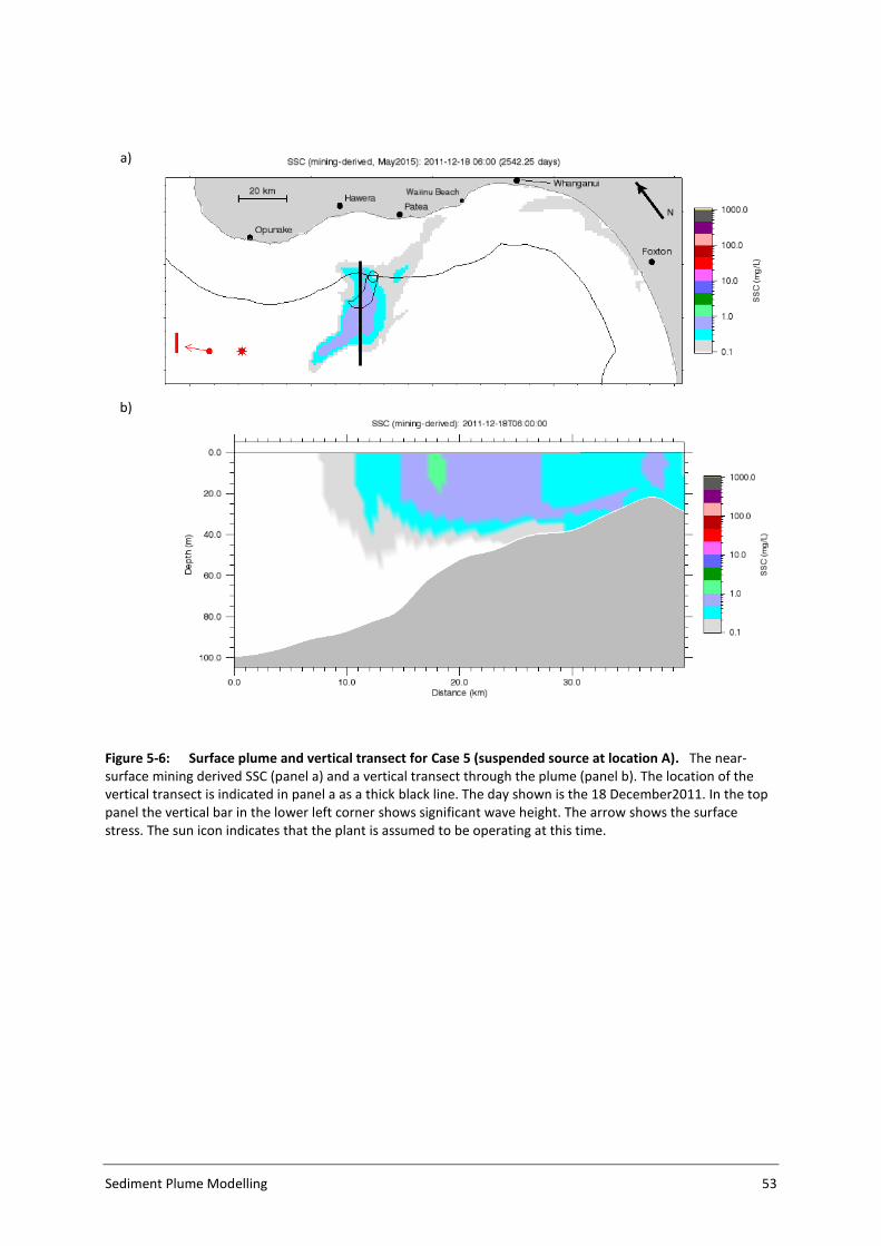
Sediment Plume Modelling 53
a)
b)
Figure 5-6: Surface plume and vertical transect for Case 5 (suspended source at location A). The near-surface mining derived SSC (panel a) and a vertical transect through the plume (panel b). The location of the vertical transect is indicated in panel a as a thick black line. The day shown is the 18 December2011. In the top panel the vertical bar in the lower left corner shows significant wave height. The arrow shows the surface stress. The sun icon indicates that the plant is assumed to be operating at this time.

54 Sediment Plume Modelling
a)
b)
Figure 5-7: Surface plume and vertical transect for Case 6 (suspended source at location A). The near-surface mining derived SSC (panel a) and a vertical transect through the plume (panel b). The location of the vertical transect is indicated in panel a as a thick black line. The day shown is the 25 July 2012. In the top panel the vertical bar in the lower left corner shows significant wave height. The arrow shows the surface stress. The sun icon indicates that the plant is assumed to be operating at this time.
5.1.2 SSC statistics
The figures in this section show maps of median and 99th percentile SSC in the model layers next to
the surface (labelled “surface” or “near-surface” SSC) and the bottom (labelled “bottom” or “near-
bottom” SSC) for the suspended source at mining location A. Figure 5-8 shows the median, near-
surface SSC. Panel a shows background SSC, from the simulation with background sediments only;
panels b and c both show results from a simulation with background and mining-derived sediments,
the former showing mining-derived sediments only and the latter the total sediment concentration.
The median, near-surface, background SSC (Figure 5-8a) was shown and discussed previously (Figure
4-8a). There is a strip of elevated values adjacent to the coast, and this strip is wider over the Patea
Shoals than it is further to the southeast. The highest values are in excess of 20 mg/L (magenta) and
occur near the mouths of the Manawatu and Whanganui Rivers. At the coast between Hawera and
Patea the SSC is typically 10–20 mg/L. At the inshore end of the Project Area the median, near-
surface, background SSC is 0.4 mg/L (light blue) and at the offshore end it is ~0.05 mg/L (white).

Sediment Plume Modelling 55
However note that from the discussion in Section 4.2 we expect that the model will underestimate
background SSC offshore and we know that it neglects suspended organic matter that will also affect
the water’s optical properties.
The map of median mining-derived SSC (Figure 5-8b) indicates that the sediment plume frequently
extends to the east-southeast from the source location towards the coast at Whanganui. The highest
values occur around the source; there is a region extending some 10 km from the source with values
between 0.5 and 1 mg/L (light purple). At 20 km downstream from the source the median SSC is
0.35 mg/L. There is an extensive area that reaches the coast with median SSC above 0.1 mg/L (light
grey). However at the shore the modelled background concentrations (panel a) exceed the mining-
derived concentrations (panel b) by approximately two orders of magnitude.
Figure 5-8 is at too large a spatial scale to clearly show SSC statistics within a few kilometres of the
source. Figure 5-12 shows an expanded view of the statistics of mining-derived SSC around the
source; from panel a we can see that the highest median, near-surface SSC in the mining plume is
1.45 mg/L.
Returning to Figure 5-8, we can compare the maps of median background SSC (panel a) and
background plus mining-derived SSC (panel c). The 1 mg/L threshold (light purple-light green) moves
some 6 km outwards over Patea Shoals to encompass the inner end of the Project Area. On a wider
scale, the transition zone that occurs in the background simulation between higher near-shore values
and lower off-shore values steps outwards perceptibly along the coast between Hawera and
Whanganui with the addition of the mining sediments.
Figure 5-9 is similar to Figure 5-8 but shows the 99th percentile near-surface SSC rather than the
median. For background sediments (panel a) this varies from a minimum of ~ 0.1 mg/L (white)
offshore from Manawatu and Horowhenua up to ~ 100 mg/L near the coast, with maxima > 200 mg/L
around the Manawatu and Whanganui Rivers. At the inshore end of the project area the 99th
percentile background SSC is 5–10 mg/L (blue) and at the offshore end it is ~ 2 mg/L.
The mining-derived SSC (panel b) shows an extensive plume with the 99th percentile between 2 and
5 mg/L (dark green) up to 30 km southeast of the source. At 20 km downstream from the source the
99th percentile SSC is 2.8 mg/L. Values at the coast southward from Patea to Whanganui are
between 1 and 2 mg/L (light green), but as with the median these are well below the natural 99th
percentile values next to the coast.
A comparison of the background plus mining derived SSCs (panel c) with the background SSCs
(panel a) shows very minor differences.
Figure 5-12b shows the expanded view of the 99th percentile mining-derived SSC around the source.
There is an irregular strip ~ 7 km long around the source where the values exceeds 5 mg/L (blue) and
the highest value is 8.25 mg/L.
Figure 5-10 shows the median, near-bottom SSC. The background value (Figure 5-10a) is typically
greater than the median, near-surface background SSC (Figure 5-8a) by a factor of 10 or more. The
highest values are in excess of 200 mg/L (magenta) and occur near the mouth of the Whanganui
River and also near Hawera. At the coast between Hawera and Patea the SSC is typically 100–
200 mg/L (salmon). At the inshore end of the Project Area the median, near-surface, background SSC
is 6 mg/L (blue) and at the offshore end it is 1.5 mg/L (light green).

56 Sediment Plume Modelling
The median, near-bottom mining-derived SSC (Figure 5-10b) shows a similar pattern to the
corresponding near-surface plot (Figure 5-8b) but with concentrations generally higher by a factor of
two. The median, mining-derived SSC is not as bottom-intensified as the median, background SSC.
There is a region extending some 20 km from the source with values between 0.5 and 1 mg/L (light
purple). There is an extensive area that reaches the coast with median SSC above 0.2 mg/L (light
blue). Near the source (Figure 5-12c) there is a pronounced peak at the source location with a
median value of 14 mg/L (whereas the median surface plume [Figure 5-12a] lacks such a peak).
Comparing background plus mining-derived SSC (panel c) and the background sediment (panel a) the
differences are very small at more than 2–3 km of the source.
Figure 5-11 shows the 99th percentile near-bottom SSC. For the background SSC (Figure 5-11a) this
statistic is 2–5 mg/L (dark green) offshore and > 500 mg/L (dark grey) along the coast, with peaks
above 1000 mg/L at the Whanganui River and along the coast near Hawera. For the mining-derived
SSC (Figure 5-11b) the plume resembles the surface 99th percentile plume (Figure 5-9b) but with
generally higher concentrations. There is an extensive area between 1 and 2 mg/L (light green)
reaching the coast from Patea to Foxton and southward along the Kapiti Coast. The highest coastal
values occur around Whanganui and are around 6–7 mg/L (blue). Near the source (Figure 5-12d) the
highest value occurs at the source location and is 45 mg/L.
There is very little difference between the background-only and background plus mining-derived
maps (panels a and c).

Sediment Plume Modelling 57
a)
b)
c)
Figure 5-8: Median near-surface concentration of suspended sediment from mining at source location A. a) Background SSC; b) mining-derived SSC; c) background plus mining-derived SSC. An open circle of 2 km radius in panels b and c indicates the source location.
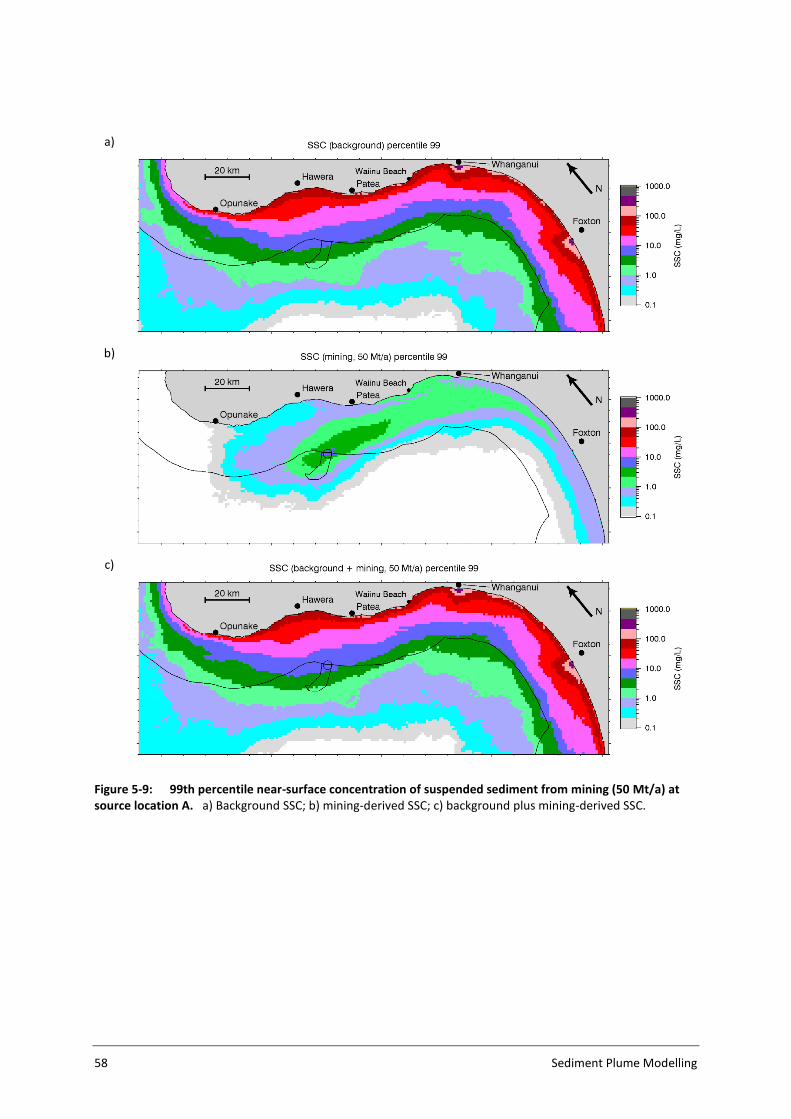
58 Sediment Plume Modelling
a)
b)
c)
Figure 5-9: 99th percentile near-surface concentration of suspended sediment from mining (50 Mt/a) at source location A. a) Background SSC; b) mining-derived SSC; c) background plus mining-derived SSC.

Sediment Plume Modelling 59
a)
b)
c)
Figure 5-10: Median near-bottom concentration of suspended sediment from mining (50 Mt/a) at source location A. a) Background SSC; b) mining-derived SSC; c) background plus mining-derived SSC.

60 Sediment Plume Modelling
a)
b)
c)
Figure 5-11: 99th percentile near-bottom concentration of suspended sediment from mining (50 Mt/a) at source location A. a) Background SSC; b) mining-derived SSC; c) background plus mining-derived SSC.

Sediment Plume Modelling 61
a)
b)
c)
d)
Figure 5-12: Near-source statistics of mining derived sediment concentration from mining source A. a) Near-surface median; b) near-surface 99th percentile; c) near-bottom median; d) near-bottom 99th percentile. A circle of 2 km radius is drawn along with a small circle indicating the centre of the source grid cell.

62 Sediment Plume Modelling
5.1.3 SSC seasonal effects
Figure 5-13 and Figure 5-14 present a three-way comparison (background; mining; background plus
mining) for median, near surface SSC but for the three summer months (December to February,
Figure 5-13), and the three winter months (June to August, Figure 5-14). They indicate that the
modelled background concentrations have a significant seasonal variation, e.g. halfway between
source location A and Patea we have 0.5–1 mg/L (light purple) in summer and 2–5 mg/L (dark green)
in winter. There is also a significant seasonal variation in mining-derived SSC, by a factor of 2–3. As a
result, the plume is somewhat more conspicuous above the background levels in summer than
winter. Even in summer, however, the mining-derived plume has no perceptible effect at the shore.

Sediment Plume Modelling 63
a)
b)
c)
Figure 5-13: Median summer (December–February) near-surface concentration of suspended sediment from mining (50 Mt/a) at source location A. a) Background SSC; b) mining-derived SSC; c) background plus mining-derived SSC.

64 Sediment Plume Modelling
a)
b)
c)
Figure 5-14: Median winter (July–August) near-surface concentration of suspended sediment from mining (50 Mt/a) at source location A. a) Background SSC; b) mining-derived SSC; c) background plus mining-derived SSC.
5.1.4 Deposition
The figures in this section show rates of sediment deposition associated with the suspended
sediment source at location A. Deposition is characterised by two statistics, the maximum 5-day
deposition (i.e. the maximum increment in thickness over any 5-day interval) and the maximum 365-
day deposition. All are evaluated over the last two years of the simulation. For each of these
deposition statistics, the increment is calculated at each grid cell separately, so that the time at
which the maximum increment is found will generally be different for each grid cell.

Sediment Plume Modelling 65
Figure 5-15 shows the maximum 5-day deposition. The organisation of this figure is similar to that
established for the SSC figures in the previous section, i.e. panel a is for background sediment in a
simulation with background sediments, panel b is for mining-derived sediments in a simulation with
both background and mining-derived sediment, and panel c is for both background and mining-
derived sediments in the same simulation as panel b. Panels a and c relate to changes in the total
thickness of the sediment bed, expressed in millimetres. For panel b, we are considering only a
subset of the sediment classes in the bed: in this case an equivalent thickness is calculated by taking
the total mass of these sediment classes in kg/m2, divided by the in situ bulk density. The latter is
equal to the grain density (3100 kg/m3 for the mining-derived sediments) divided by (1-porosity).
With the assumed porosity of 0.4, the bulk density is 1860 kg/m3.
The colour scale in the deposition figures is logarithmic and covers the range 0.01 mm to 100 mm.
Note that the lower end of this scale (0.01 mm = 10 μm) is equal to the diameter of a single fine silt
particle and is one-tenth the diameter of a typical human hair.
Background 5-day deposition values (Figure 5-15a) are typically 0.2–2 mm (dark green to magenta)
inside the territorial limit and 0.01–0.2 mm (light grey to light green) further offshore. Near the coast
they exceed 2 mm in places.
The mining-derived 5-day deposition figure (Figure 5-15b) shows an extensive plume with very low
thicknesses, between 0.01 and 0.05 mm (light grey and light blue). The highest value occurs at the
source (Figure 5-17a) and is 0.6 mm. Note that this relates not to material that is deposited in the pit
(and maybe subsequently buried) but to material that is deposited on the surrounding seabed.
The background plus mining figure (Figure 5-15c) is indistinguishable from the background only figure
(Figure 5-15a) except (when the figure is magnified) in the 1 km grid cell around the source.
Figure 5-16 shows the maximum 365-day deposition. For the background sediments (panel a) there is
an area shaded white on and south of the Patea Shoals and another 15–30 km offshore near Foxton.
Over most of these areas the maximum 365-day deposition is negative, which cannot be represented
on a logarithmic scale. The negative values occur because the seabed in this area undergoes net
erosion (up to a few mm) over the course of the model run. Nevertheless the mining-derived, 365-
day deposition (Figure 5-16b) appears to be largely unaffected by the long-term erosion and
deposition trends in the background model and shows a very similar pattern to the 5-day deposition,
with somewhat larger values, typically around twice as large. The highest value occurs at the source
(Figure 5-17b) and is 1.0 mm.
Again, the background plus mining figure (Figure 5-16c) is indistinguishable from the background only
figure (Figure 5-16a) except near the source.
Figure 5-18 shows the 2-year deposition of material. The locations of high deposition over the course
of the simulation have similar patterns to the 5-day and the 365-day maximum depositions. Similarly,
the background plus mining is almost indistinguishable from the background.
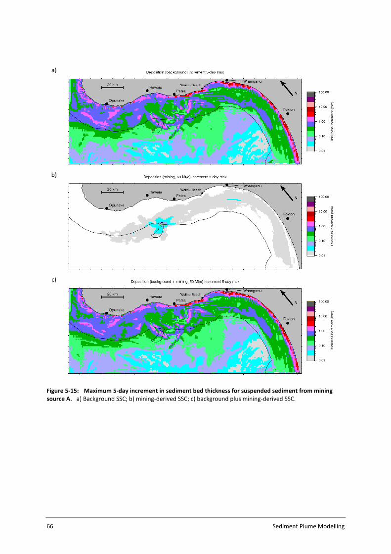
66 Sediment Plume Modelling
a)
b)
c)
Figure 5-15: Maximum 5-day increment in sediment bed thickness for suspended sediment from mining source A. a) Background SSC; b) mining-derived SSC; c) background plus mining-derived SSC.

Sediment Plume Modelling 67
a)
b)
c)
Figure 5-16: Maximum 365-day increment in sediment bed thickness for suspended sediment from mining source A. a) Background SSC; b) mining-derived SSC; c) background plus mining-derived SSC.

68 Sediment Plume Modelling
a)
b)
Figure 5-17: Near-source maximum increment of mining derived sediment, source A. a) 5-day increment; b) 365-day increment.

Sediment Plume Modelling 69
a)
b)
c)
Figure 5-18: 2-year increment in sediment bed thickness for suspended sediment from mining source A. a) Background SSC; b) mining-derived SSC; c) background plus mining-derived SSC.

70 Sediment Plume Modelling
5.2 Suspended source at mining location B
5.2.1 Selected cases
Analysis of the simulations for the suspended source at mining location B follows the pattern for
location A. The present section shows the plume of mining-derived sediment (Figure 5-19 to Figure
5-24) for the same 6 cases as Section 5.1.1. In Case 1 (Figure 5-19) sediments released from location
B do not travel southeast along the shoreline as they do with location A. For the remaining cases the
surface expression of the mining plume released from location B extends in a similar shape and
direction as the equivalent mining plume released from location A: the plume in Cases 2 (Figure 5-20)
and 4 (Figure 5-22) extends to the southeast along the shoreline; the plume in Case 3 (Figure 5-21)
pools near the release site; the plume in Case 5 (Figure 5-23) extends offshore; and in Case 6 (Figure
5-24) it extends to the east.
In the vertical, for most of the cases, the sediment plume is well mixed throughout the water column
(in a similar manner to sediments released from location A). The exception to this is Case 5 where the
plume resides in the water column between 20 and 60 m.

Sediment Plume Modelling 71
a)
b)
Figure 5-19: Surface plume and vertical transect for Case 1 (suspended source at location B). The near-surface mining derived SSC (panel a) and a vertical transect through the plume (panel b). The location of the vertical transect is indicated in panel a as a thick black line. The day shown is the 19 January 2011. In the top panel the vertical bar in the lower left corner shows significant wave height. The arrow shows the surface stress. The sun icon indicates that the plant is assumed to be operating at this time.

72 Sediment Plume Modelling
a)
b)
Figure 5-20: Surface plume and vertical transect for Case 2 (suspended source at location B). The near-surface mining derived SSC (panel a) and a vertical transect through the plume (panel b). The location of the vertical transect is indicated in panel a as a thick black line. The day shown is 14 September 2011. In the top panel the vertical bar in the lower left corner shows significant wave height. The arrow shows the surface stress. The sun icon indicates that the plant is assumed to be operating at this time.

Sediment Plume Modelling 73
a)
b)
Figure 5-21: Surface plume and vertical transect for Case 3 (suspended source at location B). The near-surface mining derived SSC (panel a) and a vertical transect through the plume (panel b). The location of the vertical transect is indicated in panel a as a thick black line. The day shown is the 22 September 2011. In the top panel the vertical bar in the lower left corner shows significant wave height. The arrow shows the surface stress. The sun icon indicates that the plant is assumed to be operating at this time.

74 Sediment Plume Modelling
a)
b)
Figure 5-22: Surface plume and vertical transect for Case 4 (suspended source at location B). The near-surface mining derived SSC (panel a) and a vertical transect through the plume (panel b). The location of the vertical transect is indicated in panel a as a thick black line. The day shown is the 2 October 2011. In the top panel the vertical bar in the lower left corner shows significant wave height. The arrow shows the surface stress. The sun icon indicates that the plant is assumed to be operating at this time.

Sediment Plume Modelling 75
a)
b)
Figure 5-23: Surface plume and vertical transect for Case 5 (suspended source at location B). The near-surface mining derived SSC (panel a) and a vertical transect through the plume (panel b). The location of the vertical transect is indicated in panel a as a thick black line. The day shown is the 18 December 2011. In the top panel the vertical bar in the lower left corner shows significant wave height. The arrow shows the surface stress. The sun icon indicates that the plant is assumed to be operating at this time.

76 Sediment Plume Modelling
a)
b)
Figure 5-24: Surface plume and vertical transect for case61 (suspended source at location B). The near-surface mining derived SSC (panel a) and a vertical transect through the plume (panel b). The location of the vertical transect is indicated in panel a as a thick black line. The day shown is the 25 July 2012. In the top panel the vertical bar in the lower left corner shows significant wave height. The arrow shows the surface stress. The sun icon indicates that the plant is assumed to be operating at this time.
5.2.2 SSC statistics
The following five figures (Figure 5-25 to Figure 5-29) are similar to the corresponding figures (Figure
5-8 to Figure 5-12) in Section 5.1.2 but for mining location B.
In Figure 5-25, showing median, near-surface SSC, panel a (background sediments) is identical to
Figure 5-8a. Panel b (mining-derived sediments) can be compared with Figure 5-8a and shows a
similar plume extending to the east-southeast, but displaced further offshore and with much lower
concentrations. For source B, the 0.1 mg/L contour (the white to light grey transition) extends some
40 km downstream and does not reach the coastline as it did for source A.
Comparing maps of median background SSC (Figure 5-25a) and background plus mining-derived SSC
(Figure 5-25c) shows a perceptible difference, with the light blue to light purple boundary (0.5 mg/L)
extending some 15 km further offshore in panel c to encompass the source location.
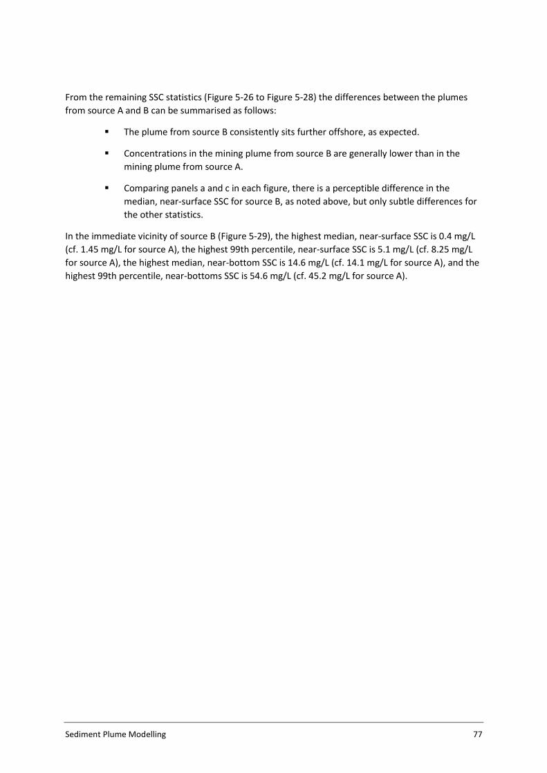
Sediment Plume Modelling 77
From the remaining SSC statistics (Figure 5-26 to Figure 5-28) the differences between the plumes
from source A and B can be summarised as follows:
The plume from source B consistently sits further offshore, as expected.
Concentrations in the mining plume from source B are generally lower than in the
mining plume from source A.
Comparing panels a and c in each figure, there is a perceptible difference in the
median, near-surface SSC for source B, as noted above, but only subtle differences for
the other statistics.
In the immediate vicinity of source B (Figure 5-29), the highest median, near-surface SSC is 0.4 mg/L
(cf. 1.45 mg/L for source A), the highest 99th percentile, near-surface SSC is 5.1 mg/L (cf. 8.25 mg/L
for source A), the highest median, near-bottom SSC is 14.6 mg/L (cf. 14.1 mg/L for source A), and the
highest 99th percentile, near-bottoms SSC is 54.6 mg/L (cf. 45.2 mg/L for source A).
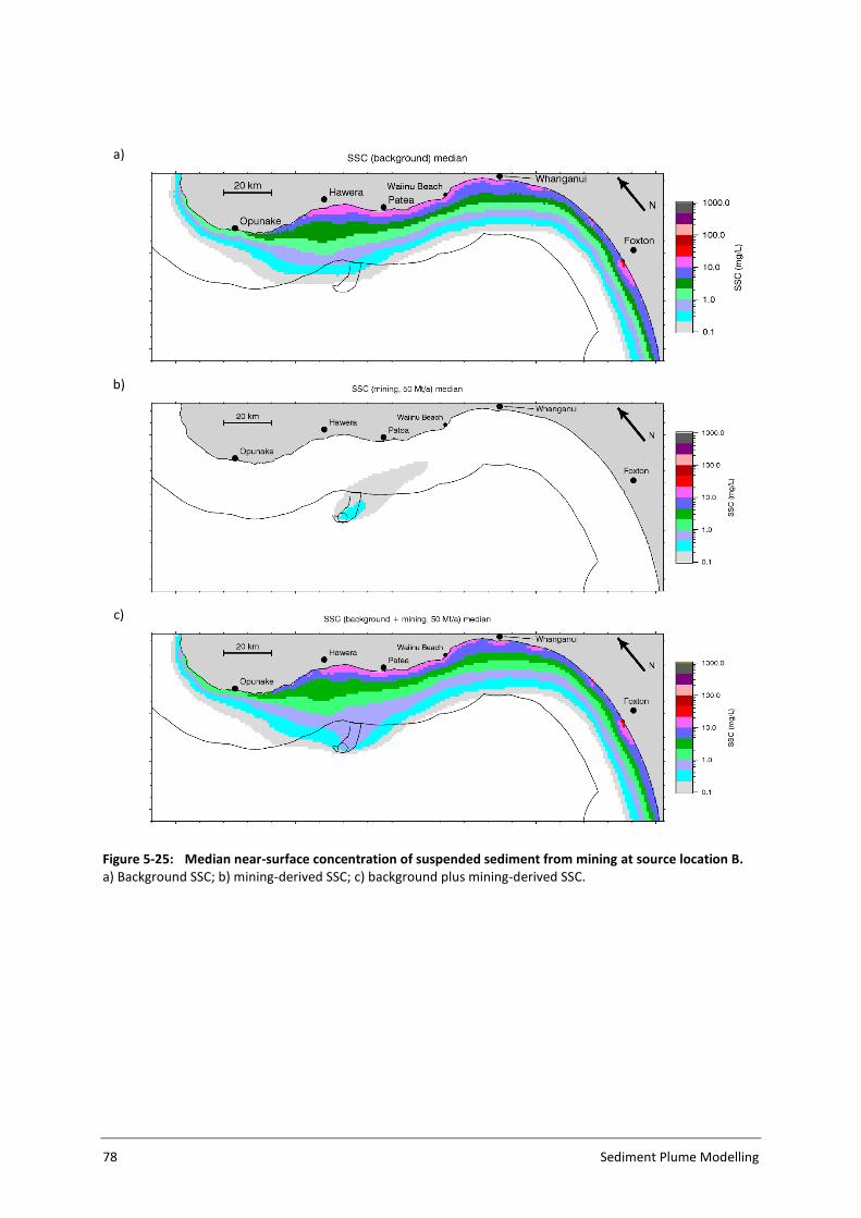
78 Sediment Plume Modelling
a)
b)
c)
Figure 5-25: Median near-surface concentration of suspended sediment from mining at source location B. a) Background SSC; b) mining-derived SSC; c) background plus mining-derived SSC.
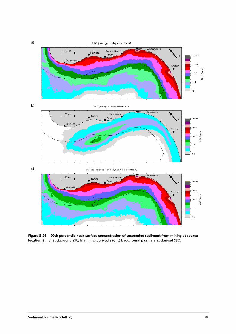
Sediment Plume Modelling 79
a)
b)
c)
Figure 5-26: 99th percentile near-surface concentration of suspended sediment from mining at source location B. a) Background SSC; b) mining-derived SSC; c) background plus mining-derived SSC.

80 Sediment Plume Modelling
a)
b)
c)
Figure 5-27: Median near-bottom concentration of suspended sediment from mining at source location B. a) Background SSC; b) mining-derived SSC; c) background plus mining-derived SSC.

Sediment Plume Modelling 81
a)
b)
c)
Figure 5-28: 99th percentile near-bottom concentration of suspended sediment from mining at source location B. a) Background SSC; b) mining-derived SSC; c) background plus mining-derived SSC.

82 Sediment Plume Modelling
a)
b)
c)
d)
Figure 5-29: Near-source statistics of mining derived sediment concentration from mining source B. a) Near-surface median; b) near-surface 99th percentile; c) near-bottom median; d) near-bottom 99th percentile.

Sediment Plume Modelling 83
5.2.3 Deposition
The deposition figures for source B (Figure 5-30 to Figure 5-32) are similar to those shown for
source A (Figure 5-15 to Figure 5-17) and similar overall behaviour is evident:
The mining deposition footprint, as indicated by the maximum 5-day and 365-day
increments in sediment thickness (panel c), is extensive but at very low values, 0.01 to
0.1 mm.
The difference between the background-only (panel a) and background plus mining
(panel c) figures is very small, except within a kilometre or two of the source.
The highest 5-day and 365-day increments (Figure 5-32) for mining-derived sediment occur at the
source grid cell and are 0.7 mm and 1.4 mm, respectively, cf. 0.6 mm and 1.1 mm for source A.
84 Sediment Plume Modelling
a)
b)
c)
Figure 5-30: Maximum 5-day increment in sediment bed thickness for suspended sediment from mining source B. a) Background SSC; b) mining-derived SSC; c) background plus mining-derived SSC.
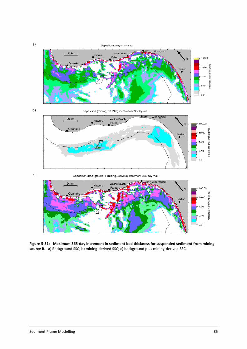
Sediment Plume Modelling 85
a)
b)
c)
Figure 5-31: Maximum 365-day increment in sediment bed thickness for suspended sediment from mining source B. a) Background SSC; b) mining-derived SSC; c) background plus mining-derived SSC.

86 Sediment Plume Modelling
a)
b)
Figure 5-32: Near-source maximum increment of mining derived sediment, source B. a) 5-day increment; b) 365-day increment.

Sediment Plume Modelling 87
5.3 Patch source
The patch source is a 3 × 2 km rectangular area representing one year’s worth of de-ored sand
deposited on the sea floor at mining location A. The patch is put in place at 2200 days and the
simulation continues for another 800 days (this being the length of simulation available). Due to
trapping of fine sediments in the tailings, the fine sediment concentration in the patch is somewhat
elevated relative to the surrounding seabed. In the patch simulation we follow the transport and
redeposition of this fine sediment.
Figure 5-33 shows the thickness of patch sediment immediately after placement, then after another
730 days. A black rectangle indicates the patch outline. The area inside the patch is maroon,
indicating a thickness between 20 and 50 mm; in fact it is 37 mm, this being the total equivalent
thickness of fine sediment in the seabed (which is arbitrarily assumed to be 1 m thick). Initially there
is no sediment outside the patch. After 730 days, patch material is found on the surrounding seabed
at thicknesses > 0.01 mm up to 10 km from the patch boundary, with a slight bias to the southeast,
and the maximum thickness outside the patch boundary is 1 mm (magenta).
Figure 5-34 shows the 99th percentile of the surface concentration of fine sediments from the patch
for 0–365 and 365–730 days after patch placement. In both periods there is a plume of very low
concentrations (< 0.2 mg/L) extending up to 10 km east-southeast of the patch.
Figure 5-35 shows similar graphs of the 99th percentile, near-bottom concentration. Over the patch
the value is 3.8 mg/L (dark green). Values exceeding 0.2 mg/L (light blue) occur up to 6 km east-
southeast of the patch boundaries. The plume is a little less extensive during the second year than
during the first. For comparison, the 99th percentile, near-bottom background SSC at this location
(Figure 5-11a) is over 100 mg/L.
It is probable that this simulation is underestimating the rate at which the patch sediment is eroded
and transported, because the model’s formulation of active layer thickness does not take account of
the complex bed forms in the area (and we believe that the model underestimates the rate at which
sand is suspended at this site, though it overestimates it at other sites (this report, Section 4.3).
However, even allowing for some underestimation by the model, there is no indication that erosion
from the patch of de-ored sand will produce plumes that are comparable to those produced by the
suspended source. This is because the fine material in the patch is distributed over the depth of the
mining pit and is released only slowly into suspension as the seabed in the patch is overturned or
eroded.

88 Sediment Plume Modelling
a)
b)
Figure 5-33: Thickness of fine sediment from the patch source. a) Snapshot immediately after initialisation. b) Snapshot after 730 days. A thick, black rectangle indicates the patch outline.

Sediment Plume Modelling 89
a)
b)
Figure 5-34: 99th percentile of near-surface SSC of fine sediments from the patch. a) 0–365 days after initialisation. b) 365–730 days after initialisation.

90 Sediment Plume Modelling
a)
b)
Figure 5-35: 99th percentile of near-bottom SSC of fine sediments from the patch. a) 0–365 days after initialisation. b) 365–730 days after initialisation.

Sediment Plume Modelling 91
6 Acknowledgements Thanks to NIWA colleagues Graham Rickard, Matt Pinkerton and Alison MacDiarmid for constructive
comments on this report and the work it describes. Thanks to HR Wallingford staff Mike Dearnaley
and Jeremy Spearman for contributing their expertise on sediment dynamics. Thanks to Peter
Gerring for his work on Figure 1-1.

92 Sediment Plume Modelling
7 References Booij, N.; Ris, R.C.; Holthuijsen, L.H. (1999). A third-generation wave model for coastal
regions 1. Model description and validation. Journal of Geophysical Research 104(C4):
7649–7666.
Carton, J.A.; Giese, B.S. (2008). A reanalysis of ocean climate using simple ocean data
assimilation (SODA). Monthly Weather Review 136(8): 2999-3017.
Carter, L., Garlick, R.D., Sutton, P.J.H., Chiswell, S.M., Oien, N.A., Stanton, B.R. (1998) Ocean
circulation New Zealand. NIWA Chart Miscellaneous Series No. 76.
Dean, R.G.; Dalrymple, R.A. (1991). Water Wave Mechanics for Engineers and Scientists.
ISBN 981-02-0420-5. World Scientific Publishing Co Pte. Ltd, 352 pp.
Goring, D. (2001). Computer models define tide variability. The Industrial Physicist 7(5): 14.
Goring, D.K.; Walters, R.A.; Bell, R.G. (1997). Modelling the propagation of tides around
New Zealand." Presented at the Pacific Coasts and Ports '97, Christchurch, New Zealand,
September 7-11, 1997.
Gorman, R.M.; Bryan, K.R.; Laing, A.K. (2003a). Wave hindcast for the New Zealand region:
deep water wave climate. New Zealand Journal of Marine and Freshwater Research
37(3): 589-612.
Gorman, R.M.; Bryan, K.R.; Laing, A.K. (2003b). Wave hindcast for the New Zealand region:
nearshore validation and coastal wave climate. New Zealand Journal of Marine and
Freshwater Research 37(3): 567–588.
HR Wallingford (2015). Support to Trans-Tasman Resources: Source Terms and Sediment
Properties for Plume Dispersion Modelling. DDM7316-RT004-01. 88 p.
Walters, R.A.; Goring, D.G.; Bell, R.G. (2001). Ocean tides around New Zealand. New
Zealand Journal of Marine and Freshwater Research 35: 567–579.
Hadfield, M.G. (2013). South Taranaki Bight Iron Sand Extraction Sediment Plume
Modelling: Phase 3 studies. NIWA Client Report WLG2013-36, 86 p.
http://www.epa.govt.nz/Publications/NIWA_sediment_plume_modelling_report.pdf
Hadfield, M.G. (2014a). Statement of Evidence of Mark Gregory Hadfield on behalf of Trans-
Tasman Resources Ltd, 56 p. http://www.epa.govt.nz/eez/EEZ000004/
EEZ000004_20_Mark%20Hadfield_(Sediment%20plume%20modelling).PDF
Hadfield, M.G. (2014b). South Taranaki Bight Sediment Plume Modelling: the Effect of
Revised Source Particle-Size Distributions, 11 p. http://www.epa.govt.nz/eez/
EEZ000004/EEZ000004_Hadfield%20-%20Revised%20Particle%20Size%20
Simulations%20-%2019%20March.pdf
Hadfield, M.G. (2014c). South Taranaki Bight Sediment Plume Modelling: Solute Dilution in
the Hydrocyclone Overflow Plume, 4 p. http://www.epa.govt.nz/eez/EEZ000004/
EEZ000004_Hadfield%20-%20Solute%20Dilution%20Report%20-%2020%20March.pdf
HR Wallingford (2015). Reference to be supplied by HRW.

Sediment Plume Modelling 93

94 Sediment Plume Modelling
Kalnay, E.; Kanamitsu, M.; Kistler, R.; Collins, W.; Deaven, D.; Gandin, L.; Iredell, M.; Saha,
S.; White, G.; Woollen, J.; Zhu, Y.; Leetmaa, A.; Reynolds, R.W.; Chelliah, M.; Ebisuzaki,
W.; Higgins, W.; Janowiak, J.; Mo, K.C.; Ropelewski, C.; Wang, J.; Jenne, R.; Joseph, D.
(1996). The NCEP/NCAR 40-Year Reanalysis Project. Bulletin of the American
Meteorological Society 77(3): 437–471. doi:10.1175/1520-
0477(1996)077<0437:TNYRP>2.0.CO;2
MacDiarmid, A.; Anderson, O.; Beaumont, J.; Gorman, R.; Hancock, N.; Julian, K.; Schwarz,
J.; Stevens, C.; Sturman, J.; Thompson, D.; Torres, L. (2010). South Taranaki Bight iron
sand mining baseline environmental study. NIWA client report WLG2010-46.
MacDonald, I.T., Budd, R., Bremner, D., Edhouse, S. (2012). South Taranaki Bight Iron Sand
Mining: Oceanographic measurements data report. NIWA Client Report, HAM2012-147:
109 pp.
MacDonald, I.T.; Gall, M.; Bremner, D. (2013). Nearshore Optical Water Quality in the South
Taranaki Bight. NIWA Client Report HAM2013-040, 88 p. http://www.epa.govt.nz/
Publications/Nearshore_Measurements_of_Optics_and_SSC_Final.pdf
Manning, A.J.; Baugh, J.V.; Soulsby, R.V.; Spearman, J.R.; Whitehouse, J.S. (2011). Cohesive
Sediment Flocculation and the Application to Settling Flux Modelling. In: Ginsberg, S.S.
(ed.). Sediment Transport, 27 pp. http://www.intechopen.com/books/sediment-
transport/cohesive-sediment-flocculation-and-the-application-to-settling-flux-modelling
Marchesiello, P.; McWilliams, J.C.; Shchepetkin, A.F. (2001). Open boundary conditions for
long-term integration of regional oceanic models. Ocean Modelling 3(1-2): 1-20.
doi:10.1016/S1463-5003(00)00013-5
Pinkerton, M.H. (2015a). Sinking rates and source rates in the revised hydrodynamic
modelling. Memo to HRW and TTR dated 19 February 2015. 8 p.
Pinkerton, M.H. (2015b). Sinking rates and source rates in the revised hydrodynamic
modelling. Memo to HRW and TTR dated 12 March 2015. 8 p.
Pinkerton, M.H.; M. Gall (2015). Optical effects of proposed iron-sand mining in the South
Taranaki Bight region. NIWA client report WLG2015-26 for Trans-Tasman Resources.
Project TTR15301.
Pinkerton, M.H., Schwartz, J.N., Gall, M., Beaumont, J. (2013) Satellite ocean-colour remote
sensing of the South Taranaki Bight from 2002 to 2012. NIWA Client Report WLG2013-
14. 79 pp. http://www.epa.govt.nz/eez/EEZ000004/EEZ000004_Satellite_ocean_-
colour_remote_sensing_of_the_South_Taranaki_Bight_from_2002_to_2012_NIWA_Oct
ober_2013.pdf
Rickard, G.J.; Hadfield, M.G.; Roberts, M.J. (2005). Development of a regional ocean model
for New Zealand. New Zealand Journal of Marine and Freshwater Research 39: 1171–
1191.
Stanton, B.R., Goring, D.G., Bell, R.G. (2001) Observed and modelled tidal currents in the
New Zealand region. New Zealand Journal of Marine and Freshwater Research, 35(2):
397–415. 10.1080/00288330.2001.9517010

Sediment Plume Modelling 95
Thompson, R.O.R.Y. (1983) Low-Pass Filters to Suppress Inertial and Tidal Frequencies.
Journal of Physical Oceanography, 13(6): 1077-1083. doi:10.1175/1520-
0485(1983)013<1077:LPFTSI>2.0.CO;2
Trans-Tasman Resources Ltd (2013). South Taranaki Bight Iron Sands Project Impact
Assessment Summary. 16 p. http://www.epa.govt.nz/Publications/TTR_Impact_
Assessment_Summary_FINAL_21_October.pdf
Walters, R.A.; Gillibrand, P.A.; Bell, R.G.; Lane, E.M. (2010). A study of tides and currents in
Cook Strait, New Zealand. Ocean Dynamics 60(6): 1559-1580.
Warner, J.C.; Sherwood, C.R.; Signell, R.P.; Harris, C.K.; Arango, H.G. (2008). Development of
a three-dimensional, regional, coupled wave, current, and sediment-transport model.
Computers & Geosciences 34(10): 1284–1306.

96 Sediment Plume Modelling
Appendix A The ROMS vertical grid There are several references throughout this report to surface and bottom (or near-surface and near-
bottom) values of quantities like suspended sediment concentration and horizontal velocity. These
refer to vertical averages over the model layers adjacent to the surface and the bottom, respectively.
The ROMS vertical grid layout is indicated in Figure A-1.
Figure A-1: ROMS vertical grid schematic. The blue lines represent the boundaries between layers in ROMS, using the same number of layers (20) and the same vertical stretching parameters as the inner model. The depth (black line) is and idealised depth profile.
The layers are distributed between the bottom and the surface (and follow the surface as it rises and
falls with the tide). The vertical spacing is reduced near the surface and the bottom, with adjustable
parameters controlling the degree of this reduction. The thickness of the near-surface and near-
bottom layers is therefore dependent on water depth. Sample values are shown in Table A-1.
Table A-1: Inner model layer thicknesses. Thickness of the near-surface and near-bottom layers, along with maximum layer thickness as a function of water depth for the inner model.
Water depth (m)
Near-surface layer thickness (m)
Maximum layer thickness
(m)
Near-bottom layer thickness (m)
10 0.27 0.63 0.40
20 0.39 1.36 0.74
30 0.46 2.10 1.07
40 0.53 2.85 1.38
50 0.58 3.61 1.70

Sediment Plume Modelling 97
Appendix B Model-measurement comparisons For information about measurement sites and deployments, see Figure 1-1 and Table 3-1.
Tidal velocity comparison
Figure B-1: Tidal ellipse comparison (all ADCP deployments). Mid-depth M2 ellipses from measurements (blue) and model (red). The ellipses represent the magnitude and orientation of the tidal velocity variations and the straight line from the origin to the ellipse represents the phase.
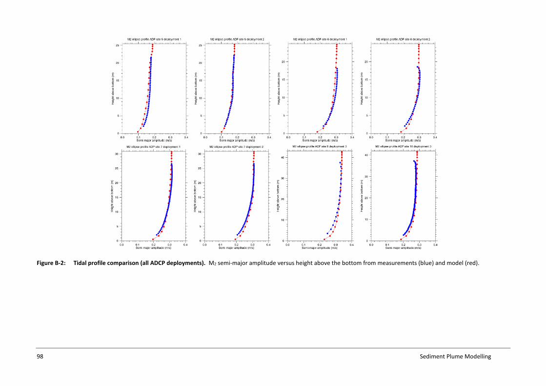
98 Sediment Plume Modelling
Figure B-2: Tidal profile comparison (all ADCP deployments). M2 semi-major amplitude versus height above the bottom from measurements (blue) and model (red).

Sediment Plume Modelling 99
Table B-1: Comparison of Mtidal ellipse parameters. Mid-depth M2 tidal ellipse parameters from ADCP measurements and model. Here “ratio” means model value divided by measured value and “diffce” means model value minus measured value.
ADCP Site/Deployment
Semi-major axis (m/s) Eccentricity Inclination (°T) Phase (°)
Meas. Model Ratio Meas. Model Diffce Meas. Model Diffce Meas. Model Diffce
Site 5 Deployment 1 0.17 0.16 0.94 0.02 -0.02 -0.04 113.5 120.9 7.4 210.3 211.1 0.8
Site 5 Deployment 2 0.17 0.17 0.98 0.02 0.00 -0.02 112.5 120.9 8.4 205.8 207.8 2.0
Site 6 Deployment 1 0.30 0.29 0.99 0.12 0.08 -0.04 129.1 132.4 3.3 198.6 196.2 -2.4
Site 6 Deployment 2 0.29 0.30 1.01 0.12 0.10 -0.01 130.4 132.7 2.3 197.3 197.3 0.0
Site 7 Deployment 1 0.30 0.30 0.98 0.16 0.15 -0.01 128.9 134.0 5.1 201.1 199.3 -1.8
Site 7 Deployment 2 0.30 0.30 1.02 0.18 0.18 -0.01 130.8 133.5 2.7 199.2 200.3 1.0
Site 8 Deployment 3 0.33 0.33 1.00 0.18 0.17 -0.01 133.4 132.2 -1.1 206.0 205.0 -1.0
Site 10 Deployment 3 0.27 0.28 1.02 0.17 0.15 -0.02 130.2 137.6 7.3 203.5 201.2 -2.2
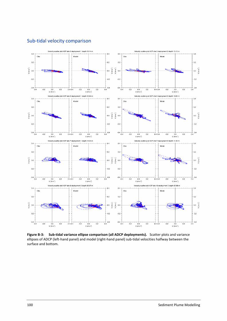
100 Sediment Plume Modelling
Sub-tidal velocity comparison
Figure B-3: Sub-tidal variance ellipse comparison (all ADCP deployments). Scatter plots and variance ellipses of ADCP (left-hand panel) and model (right-hand panel) sub-tidal velocities halfway between the surface and bottom.
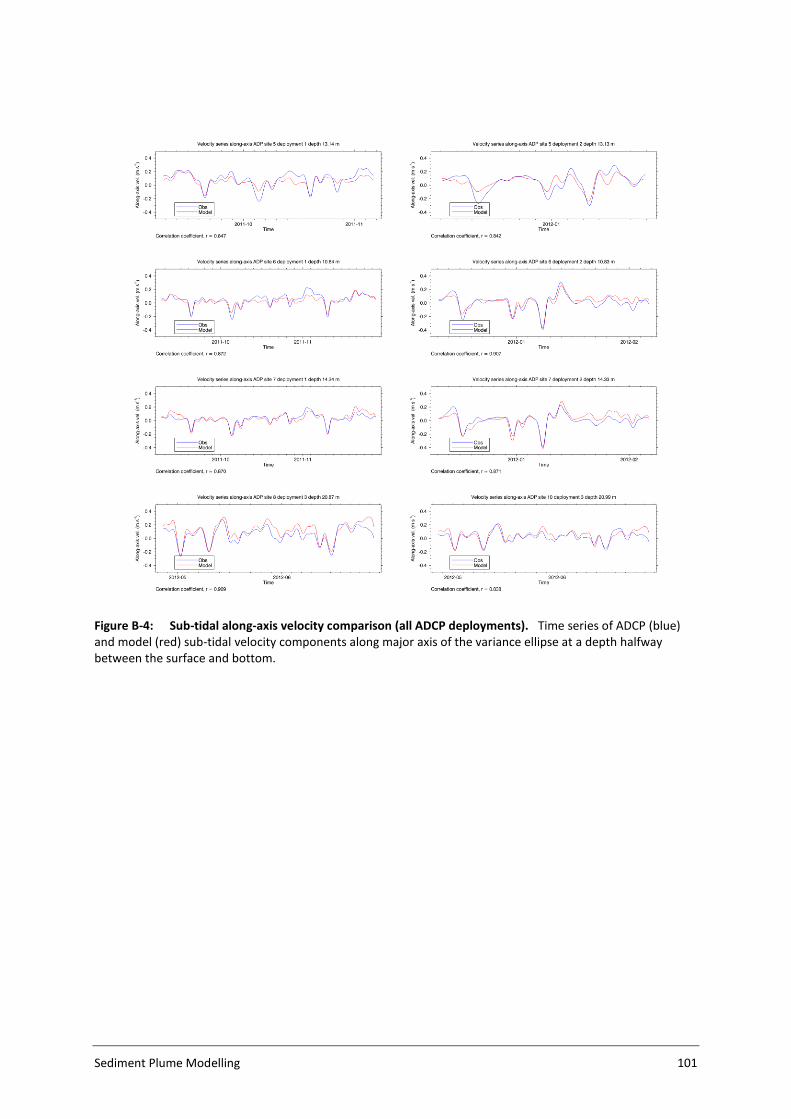
Sediment Plume Modelling 101
Figure B-4: Sub-tidal along-axis velocity comparison (all ADCP deployments). Time series of ADCP (blue) and model (red) sub-tidal velocity components along major axis of the variance ellipse at a depth halfway between the surface and bottom.

102 Sediment Plume Modelling
Figure B-5: Sub-tidal across-axis velocity comparison (all ADCP deployments). Time series of ADCP (blue) and model (red) sub-tidal velocity components perpendicular to the major axis of the variance ellipse at a depth halfway between the surface and bottom.

Sediment Plume Modelling 103
Table B-2: Mid-depth sub-tidal velocity comparison. Mid-depth sub-tidal mean and variance ellipse parameters from ADCP measurements and model, and temporal correlations between measured and modelled time series. Here “ratio” means model value divided by measured value and “diffce” means model value minus measured value
ADCP Site & Deployment
Mean magnitude (m/s)
Mean direction (°T)
Semi-major axis (m/s)
Eccentricity Inclination (°T)
Correlation
Meas. Model Diffce Meas. Model Diffce Meas. Model Ratio Meas. Model Diffce Meas. Model Diffce Along- axis
Across-axis
Site 5 Deployment 1 0.08 0.05 -0.03 97.5 103.2 5.7 0.11 0.06 0.60 0.09 0.15 0.06 95.9 100.5 4.5 0.90 0.38
Site 5 Deployment 2 0.04 0.04 0.00 93.5 103.3 9.8 0.13 0.09 0.68 0.1.0 0.17 0.07 97.0 103.8 6.9 0.93 -0.06
Site 6 Deployment 1 0.05 0.03 -0.02 105.1 104.3 -0.8 0.08 0.05 0.66 0.15 0.19 0.04 106.8 105.0 -1.8 0.88 0.56
Site 6 Deployment 2 0.01 0.02 0.01 108.0 97.0 -11.0 0.11 0.08 0.77 0.16 0.20 0.04 110.5 105.8 -4.7 0.89 0.55
Site 7 Deployment 1 0.03 0.03 0.00 69.1 67.1 -2.0 0.07 0.06 0.88 0.31 0.22 -0.09 95.0 94.3 -0.7 0.87 0.69
Site 7 Deployment 2 0.01 0.01 0.00 35.7 26.7 -8.9 0.10 0.10 1.00 0.22 0.24 0.01 104.0 102.6 -1.4 0.85 0.55
Site 8 Deployment 3 0.06 0.09 0.04 111.2 101.7 -9.5 0.11 0.1 0.93 0.26 0.22 -0.04 98.5 91.7 -6.8 0.92 0.84
Site 10 Deployment 3 0.02 0.03 0.01 111.8 97.5 -14.3 0.07 0.07 0.91 0.42 0.39 -0.04 98.7 96.8 -1.9 0.86 0.72

104 Sediment Plume Modelling
Table B-3: Near-surface subtidal velocity comparison. As Table B-2 but for an ADCP level 5 m below the surface.
ADCP Site & Deployment
Mean magnitude (m/s)
Mean direction (°T)
Semi-major axis (m/s)
Eccentricity Inclination (°T)
Correlation
Meas. Model Diffce Meas. Model Diffce Meas. Model Ratio Meas. Model Diffce Meas. Model Diffce Along- axis
Across-axis
Site 5 Deployment 1 0.12 0.1 -0.02 102.9 100.3 -2.6 0.12 0.09 0.72 0.13 0.16 0.03 96.3 100.0 3.6 0.92 0.43
Site 5 Deployment 2 0.07 0.08 0.01 110.2 107.6 -2.6 0.17 0.13 0.77 0.11 0.15 0.04 90.4 95.1 4.7 0.95 0.72
Site 6 Deployment 1 0.05 0.04 -0.01 111.1 106.3 -4.9 0.09 0.07 0.77 0.17 0.2 0.03 105.6 106.1 0.5 0.89 0.68
Site 6 Deployment 2 0.02 0.03 0.01 117 111.1 -5.9 0.12 0.10 0.88 0.17 0.25 0.07 110.6 106.4 -4.1 0.88 0.39
Site 7 Deployment 1 0.04 0.05 0.01 77.8 77.7 -0.1 0.08 0.08 1.08 0.35 0.25 -0.10 94.0 97.7 3.7 0.86 0.76
Site 7 Deployment 2 0.01 0.02 0.00 48.4 59.9 11.5 0.11 0.13 1.16 0.29 0.21 -0.08 104.3 103.4 -1.0 0.87 0.58
Site 8 Deployment 3 0.05 0.11 0.06 98.6 96.6 -2.0 0.12 0.13 1.10 0.29 0.28 -0.01 98.4 95.2 -3.1 0.94 0.89
Site 10 Deployment 3 0.03 0.05 0.02 106.7 83.3 -23.4 0.08 0.09 1.12 0.39 0.41 0.02 96.9 99.0 2.1 0.64 0.66

Sediment Plume Modelling 105
Table B-4: Near-bottom subtidal velocity comparison. As Table B-2 but for the lowest ADCP level.
ADCP Site & Deployment
Mean magnitude (m/s)
Mean direction (°T)
Semi-major axis (m/s)
Eccentricity Inclination (°T)
Correlation
Meas. Model Diffce Meas. Model Diffce Meas. Model Ratio Meas. Model Diffce Meas. Model Diffce Along- axis
Across-axis
Site 5 Deployment 1 0.05 0.02 -0.02 88.3 97.2 8.9 0.07 0.04 0.58 0.16 0.27 0.11 104.4 116.4 12.0 0.83 0.61
Site 5 Deployment 2 0.02 0.02 0.00 26.7 22.5 -4.2 0.08 0.05 0.61 0.17 0.22 0.05 117.5 127.6 10.1 0.89 0.88
Site 6 Deployment 1 0.03 0.02 -0.01 107.1 105.6 -1.5 0.06 0.04 0.56 0.15 0.28 0.13 108.8 103.9 -5.0 0.85 0.28
Site 6 Deployment 2 0.01 0.01 0.00 278.4 87.1 168.6 0.08 0.05 0.68 0.18 0.33 0.15 112.9 103 -9.9 0.90 0.42
Site 7 Deployment 1 0.02 0.02 0.00 69.0 62.1 -7.0 0.05 0.04 0.83 0.33 0.24 -0.08 99.2 93.1 -6.1 0.90 0.29
Site 7 Deployment 2 0.01 0.01 0.00 298.0 22.2 84.2 0.07 0.07 0.96 0.26 0.3 0.04 108.4 99.9 -8.6 0.88 0.33
Site 8 Deployment 3 0.04 0.07 0.03 126.2 108.9 -17.3 0.08 0.08 0.96 0.32 0.24 -0.08 102.2 92.0 -10.2 0.93 0.57
Site 10 Deployment 3 0.02 0.02 0.00 164.5 145.9 -18.6 0.06 0.04 0.74 0.5 0.52 0.02 123.8 101.3 -22.5 0.81 0.39

106 Sediment Plume Modelling
Appendix C Comparison with March 2014 model results a)
b)
Figure C-1: Comparison of median near-surface SSC due to mining at source location A. a) The March 2014 “Revised PSD” configuration; b) the present configuration.

Sediment Plume Modelling 107
a)
b)
Figure C-2: Comparison of 99th percentile near-surface SSC due to mining at source location A. a) The March 2014 “Revised PSD” configuration; b) the present configuration.

108 Sediment Plume Modelling
a)
b)
Figure C-3: Comparison of median near-bottom SSC due to mining at source location A. a) The March 2014 “Revised PSD” configuration; b) the present configuration.

Sediment Plume Modelling 109
a)
b)
Figure C-4: Comparison of 99th percentile near-bottom SSC due to mining at source location A. a) The March 2014 “Revised PSD” configuration; b) the present configuration.

110 Sediment Plume Modelling
a)
b)
Figure C-5: Comparison of median near-surface SSC due to mining at source location B. a) The March 2014 “Revised PSD” configuration; b) the present configuration.

Sediment Plume Modelling 111
a)
b)
Figure C-6: Comparison of 99th percentile near-surface SSC due to mining at source location B. a) The March 2014 “Revised PSD” configuration; b) the present configuration.

112 Sediment Plume Modelling
a)
b)
Figure C-7: Comparison of median near-bottom SSC due to mining at source location B. a) The March 2014 “Revised PSD” configuration; b) the present configuration.

Sediment Plume Modelling 113
a)
b)
Figure C-8: Comparison of 99th percentile near-bottom SSC due to mining at source location B. a) The March 2014 “Revised PSD” configuration; b) the present configuration.

114 Sediment Plume Modelling
a)
b)
Figure C-9: Maximum 5-day increment in sediment bed thickness for suspended sediment due to mining at source location A. a) The March 2014 “Revised PSD” configuration; b) the present configuration.

Sediment Plume Modelling 115
a)
b)
Figure C-10: Maximum 365-day increment in sediment bed thickness for suspended sediment due to mining at source location A. a) The March 2014 “Revised PSD” configuration; b) the present configuration.

116 Sediment Plume Modelling
a)
b)
Figure C-11:: Maximum 5-day increment in sediment bed thickness for suspended sediment due to mining at source location B. a) The March 2014 “Revised PSD” configuration; b) the present configuration.

Sediment Plume Modelling 117
a)
b)
Figure C-12: Maximum 365-day increment in sediment bed thickness for suspended sediment due to mining at source location B. a) The March 2014 “Revised PSD” configuration; b) the present configuration.