Sedimentation Effects on Triangular Short-CrestedFlow-Measurement Weirs

Fred L. Ogden, M.ASCE1; Jesse N. Creel2; Edward W. Kempema3; and Trey D. Crouch4

Abstract: Flow-measurement weirs in natural channels experience sedimentation. Removing accumulated sediment is often impractical,prohibitively expensive, or both. This paper describes the results of hundreds of laboratory experiments conducted over a 6-year period toquantify the effect of sedimentation on the discharge coefficients for short-crested 120° and 140° triangular weirs over a range of flows,channel slopes, and different measurement positions along and across the channel. Two weir crest geometries were tested. These included theU.S. Department of Agriculture, Agricultural Research Service (ARS) design, and a modified ARS-type weir crest intended to reduce thefrequency of plugging by floating debris called the Panama crest design. Two different weir crest thicknesses were tested in a hydraulicslaboratory in two different flumes, with and without horizontal planar sedimentation, to identify the effects of sedimentation on dischargecoefficients. Sediment transport was not considered. Results showed that in all cases sedimentation reduced the discharge coefficient by up to10%. Channel slope had a relatively minor effect provided that the channel slope was less than or equal to 2% with a horizontal planarbed above the weir. Depth measurement position was of minor importance provided that the measurement was made out of the region ofdrawdown near the weir. The findings reported in this paper extend the usefulness of short-crested triangular weirs to conditions where theupstream pool is filled with sediment to the weir invert. DOI: 10.1061/(ASCE)HE.1943-5584.0001528. © 2017 American Society of CivilEngineers.

Introduction

Weirs are generally of two types. The first type are constructedmidchannel, oriented perpendicular to the flow, and are calledmeasuring weirs (USBR 2001). The second type are oriented par-allel to the flow on the sides of channels and only allow water toflow out when the water in the main channel reaches a certainheight. Weirs of this second type are called side-channel weirs andare commonly used in storm drains and sewers. This study focusedon measuring weirs.

Weirs are classified by their profile normal to the flow and crestgeometry. Common weir profiles include rectangular, triangular,trapezoidal, logarithmic, and parabolic in the case of vertical road-way curves. There are three types of weir crests: sharp-edged,broad-crested, and short-crested. Sharp-edged weirs are generallymade of a thin metal plate with a machined knifelike edge at thepoint in contact with the flow. Sharp-edged weirs are difficult tomaintain in riverine settings because they are susceptible to damageby impacts by debris or ice. Broad-crested weirs are much thickerthan sharp-edged weirs, often made of concrete, with weir crestslong enough in the flow direction for the flow streamlines to

become straight and parallel over the crest. Short-crested weirs arealso frequently made of concrete and represent an intermediatecrest length that is short enough in the flow direction that stream-lines do not become parallel to the structure. In this paper, the termshort-crested is used as per this definition. However, the termsbroad-crested and short-crested have been used interchangeably(USBR 2001).

Agricultural Research Service-Type Triangular Weirs

This study was focused on triangular weirs of the AgriculturalResearch Service (ARS) variety with isosceles trapezoidal–shapedcrowns, albeit with variable crest geometry. Triangular weirs arealso called V-notch weirs. Fig. 1 shows the short-crested ARS-typeweir geometric variables and crest dimensions. The ARS recom-mendation for short-crested weir thickness is 0.41 m (16 in.)(Brakensiek et al. 1979). Unlike the knifelike crest of sharp-edgedweirs, the crowns of broad-crested and short-crested weirs can havedifferent shapes owing to their thickness. Triangular weirs can befurther classified by the angle of the V, which is shown as θ in Fig. 1.Triangular weir angles between 60° and 140° are most common.This study focused on 120° and 140° triangular short-crested weirswith isosceles trapezoidal crowns as shown in Section A-A in Fig. 1,because weirs of this geometry are commonly used in field settings.

With reference to Fig. 1, the theoretical equation for calculatingthe discharge, Q, over a triangular weir is

Q ¼ Cd8

15

ffiffiffiffiffi2g

ptan

�θ2

��hþ α

V2

2g

�5=2

ð1Þ

Eq. (1) can be solved for the discharge coefficient as

Cd ¼Q̄

815

ffiffiffiffiffi2g

ptanðθ

2ÞH̄5=2

total

ð2Þ

where Htotal ¼ hþ αV2=2g is the total head assuming that theinvert of the weir is at elevation z ¼ 0. The overbar symbol above

1Cline Distinguished Chair of Engineering, Environment, andNatural Resources, Dept. of Civil and Architectural Engineering, Univ. ofWyoming, Laramie, WY 82071 (corresponding author). E-mail: fogden@uwyo.edu

2Consulting Engineer, Englewood, CO 80110; formerly, GraduateStudent, Univ. of Wyoming, Laramie, WY 82071.

3Research Scientist, Dept. of Civil and Architectural Engineering,Univ. of Wyoming, Laramie, WY 82071.

4Ph.D. Candidate, Dept. of Environmental Engineering Sciences,Univ. of Florida, Gainesville, FL 32611; formerly, Graduate Student,Univ. of Wyoming, Laramie, WY 82071.

Note. This manuscript was submitted on May 25, 2016; approved onJanuary 25, 2017; published online on May 2, 2017. Discussion periodopen until October 2, 2017; separate discussions must be submitted forindividual papers. This paper is part of the Journal of Hydrologic Engi-neering, © ASCE, ISSN 1084-0699.

© ASCE 04017020-1 J. Hydrol. Eng.

J. Hydrol. Eng., 2017, 22(8): 04017020

Dow

nloa

ded

from

asc

elib

rary

.org

by

149.

15.1

61.1

51 o

n 10

/13/

17. C

opyr

ight

ASC

E. F

or p

erso

nal u

se o

nly;

all

righ

ts r

eser

ved.

the variables Q and Htotal indicate that those variables are the resultof repeat measurements, allowing minimization of the effects ofmeasurement errors of Q and Htotal on the dependent variable, Cd.Weirs in natural channels create local hydraulic control and providethe means to measure discharge through a water surface elevationmeasurement. The elevation of the weir invert, or low point of theV, is subtracted from the water surface elevation providing a statichead measurement h as shown in Fig. 1.

Effects of Sedimentation

Weirs around the world are filling with or are full of sediment. Theweir shown in Fig. 2 was constructed in Panama in 1979, is full ofsediment, and is currently being used in a study of land-use effectson tropical hydrology (Ogden et al. 2013). Note the near planarsediment accumulation to the height of the weir invert. This weiris inaccessible by equipment because it is more than 2 km from the

nearest road in a tropical forest. The objective of this study was toidentify discharge coefficients that account for horizontal planaraccumulations of sediment behind short-crested triangular weirs.

With reference to Fig. 1, the velocity head upstream from a tri-angular weir may be neglected when P, the vertical distance fromthe weir invert down to the bed of the channel on the upstream sideof the weir, is at least 60% of the design static head hmax. However,in natural channels that convey sediment, this condition is difficultto maintain. This is because the local control created by the pres-ence of the weir causes flow deceleration with a corresponding de-crease in sediment transport capacity. This results in sedimentdeposition in the pool upstream from the weir, decreasing P (Fig. 1)until P ¼ 0. Depending on the sediment size and transport rate,weirs can fill with sediment during a single event. Further depend-ing on site access and local conditions, routine removal of this ac-cumulated sediment may be prohibitively expensive or impossible.

Literature Review

Numerous sources discourage using triangular weirs when theapproach pool is filled with sediment up to the weir invert elevation.There are inconsistent recommendations regarding acceptablesediment accumulations. Guidance from the U.S. Bureau ofReclamation (2001) is that approach flow channels should be freeof deposited sediment. Bos (1989) recommends that the minimumdistance from the triangular weir invert to the channel bed, P inFig. 1, should be at least 46 cm. The USDA Natural ResourcesConservation Service (NRCS) (Brakensiek et al. 1979) recom-mends the channel upstream from short-crested triangular weirs benearly straight and level for a distance of 13 m, and that P ≥0.15 m. These conditions are unlikely to persist in natural channelswith sediment transport. Both the USDA NRCS (Brakensiek et al.1979) and the U.S. Bureau of Recommendation (2001) claim thatdeposition of material immediately upstream from the weir willcause flow measurement inaccuracies that are greatest at lowmeasuring heads. Yet another guidance document from the WorldMeteorological Organization requires P ≥ 0.45 m and h=P not toexceed 0.4 (WMO 1971).

Compared with rectangular weirs, triangular weirs require morehead for the same discharge. This means that triangular weirs moreaccurately measure low flows than rectangular weirs (Brakensieket al. 1979) and are therefore more suitable for use in researchwatersheds. Short-crested triangular weirs constructed of concretewere pioneered by the USDA in the 1930s and 1940s (Huff 1938,1941a, b, 1942; Harrold and Krimgold 1943; Ree and Gwinn 1959;Holtan et al. 1962; Gwinn et al. 1968). In streams where sedimenttransport is significant, other types of devices such as supercriticalflumes and drop-box weirs are recommended (Brakensiek et al.1979). However, short-crested triangular weirs are considerablyless expensive to construct.

The USDA ARS (Brakensiek et al. 1979) gives an empiricalequation involving two empirical constants C0 and C1 to calculateCd values for the ARS (m ¼ 8, Fig. 1) weir crest for nonsedimentedconditions insofar as those conditions can be identified

Cd ¼ C0þC1 log

�HT

�ð3Þ

Eq. (3) is applied piecewise over different ranges of HT−1. Thedischarge coefficients reported in Brakensiek et al. (1979) includethe constant 8=15

ffiffiffi2

p, which is equal to 0.7542, because those con-

stants that appear in the derivation of Eq. (1) are missing from theweir equation published in Brakensiek et al. (1979). Dividing thatconstant out to adapt for this difference, Table 1 gives values of the

Fig. 1. Short-crested ARS-style triangular weir geometry definitionsketch

Fig. 2. Fully sedimented forest catchment weir in Soberania NationalPark, Panama, provided the impetus for this study (weir location:9° 12′ 32″ N, 79° 46′ 46″ W) (image by Fred L. Ogden)

© ASCE 04017020-2 J. Hydrol. Eng.

J. Hydrol. Eng., 2017, 22(8): 04017020

Dow

nloa

ded

from

asc

elib

rary

.org

by

149.

15.1

61.1

51 o

n 10

/13/

17. C

opyr

ight

ASC

E. F

or p

erso

nal u

se o

nly;

all

righ

ts r

eser

ved.

constants C0 and C1 and their piecewise ranges of applicability in aform consistent with Eq. (1).

Discharge coefficients calculated using the constants in Table 1are for nonsedimented conditions. The effect of sedimentation onARS type (m ¼ 8) weirs was studied by Mefford (1979) usinga 1∶5-scale model. However, Mefford’s study was different thanthe present study in some key ways. Mefford’s study was per-formed in a large recirculating flume with live sediment transportthat in some tests had a sand dune upstream from the weir. In othertests by Mefford (1979), the sedimented bed was sloped, which ledto supercritical flow approaching the weir crest and a rooster tailforming as flow passed over the weir, similar to the observationsof Huff (1942) who attempted tests in steep channels using a1∶5-scale model. Mefford’s study results were partially summarizedby Saxton and Ruff (1976). As will be discussed in the resultssection, scale effects were observed in the 3∶16-scale model ofthe ARS weir crest. It is likely that a model at 1∶5-scale will besimilarly affected.

Objectives

Hudson (2004) discussed the problem of sediment depositionthat affects discharge measurements using weirs and offers the

following solutions: (1) clear sediment after each flood event;(2) prevent sediment from reaching the structure; (3) derive anew calibration to reflect the deposition; or (4) redesign or replacethe structure to allow sediment to pass. In many cases Solutions 1and 4 are not reasonable because of difficulty accessing weir loca-tions and expense. Sediment traps can be effective but they alsorequire expensive dredging. Because in some cases dredging ofaccumulated sediment behind triangular weirs is impossible, a sol-ution is needed. This study focused on Solution 3.

Laboratory and Apparatus

This study was performed in the Water Resources Laboratory at theUniversity of Wyoming in two different size flumes. A small flumewas used to test weirs with T ¼ 7.62 cm (T = thickness of weircrest in the flow direction, Fig. 1), while the large flume was usedto test weirs with T ¼ 20.3 cm. These two flumes are described inthe following sections.

Small Flume

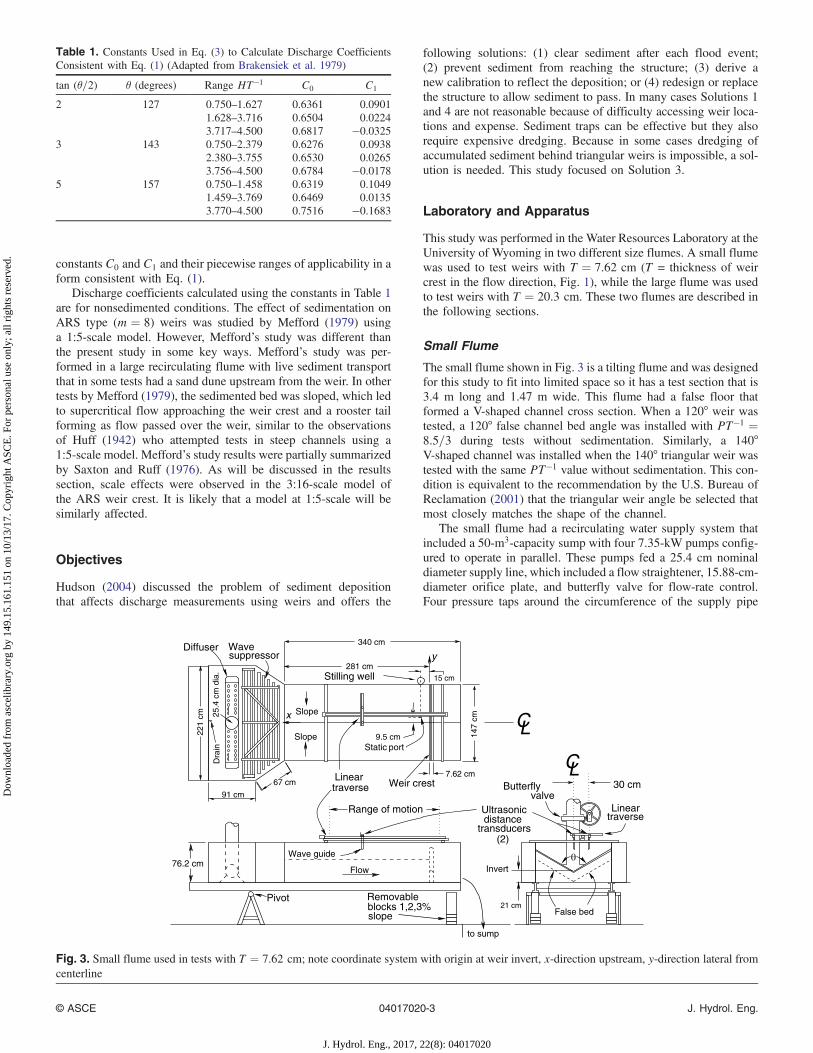
The small flume shown in Fig. 3 is a tilting flume and was designedfor this study to fit into limited space so it has a test section that is3.4 m long and 1.47 m wide. This flume had a false floor thatformed a V-shaped channel cross section. When a 120° weir wastested, a 120° false channel bed angle was installed with PT−1 ¼8.5=3 during tests without sedimentation. Similarly, a 140°V-shaped channel was installed when the 140° triangular weir wastested with the same PT−1 value without sedimentation. This con-dition is equivalent to the recommendation by the U.S. Bureau ofReclamation (2001) that the triangular weir angle be selected thatmost closely matches the shape of the channel.

The small flume had a recirculating water supply system thatincluded a 50-m3-capacity sump with four 7.35-kW pumps config-ured to operate in parallel. These pumps fed a 25.4 cm nominaldiameter supply line, which included a flow straightener, 15.88-cm-diameter orifice plate, and butterfly valve for flow-rate control.Four pressure taps around the circumference of the supply pipe

Table 1. Constants Used in Eq. (3) to Calculate Discharge CoefficientsConsistent with Eq. (1) (Adapted from Brakensiek et al. 1979)

tan (θ=2) θ (degrees) Range HT−1 C0 C1

2 127 0.750–1.627 0.6361 0.09011.628–3.716 0.6504 0.02243.717–4.500 0.6817 −0.0325

3 143 0.750–2.379 0.6276 0.09382.380–3.755 0.6530 0.02653.756–4.500 0.6784 −0.0178

5 157 0.750–1.458 0.6319 0.10491.459–3.769 0.6469 0.01353.770–4.500 0.7516 −0.1683

LC

LC221

cm

147

cm

340 cm

281 cm

25.4

cm

dia

.

91 cm

to sump

Dra

in

67 cm

76.2 cm

Slope

Slope

Ultrasonicdistance

transducers(2)

traverseLinear

Pivot

Weir crest

Removableblocks 1,2,3%slope

suppressorDiffuser Wave

Lineartraverse 30 cm

valveButterfly

Stilling well

9.5 cm

False bed

Flow

7.62 cm

portStatic

15 cm

21 cm

Invert

y

x

Wave guide

Range of motion

Fig. 3. Small flume used in tests with T ¼ 7.62 cm; note coordinate system with origin at weir invert, x-direction upstream, y-direction lateral fromcenterline

© ASCE 04017020-3 J. Hydrol. Eng.

J. Hydrol. Eng., 2017, 22(8): 04017020

Dow

nloa

ded

from

asc

elib

rary

.org

by

149.

15.1

61.1

51 o

n 10

/13/

17. C

opyr

ight

ASC

E. F

or p

erso

nal u

se o

nly;

all

righ

ts r

eser

ved.

upstream and downstream of the orifice plate were connected toa 2.3-m-tall differential water manometer. This orifice plate–manometer system was used to set flow rates at target values, andto validate operation of the weigh tank system. After overflowingthe weir, the water flowing in this flume spilled into a return troughin the laboratory floor where it traveled to the splitter box above aweigh tank system.

The splitter box contained two 25.4-cm-diameter computer-controlled pneumatically actuated butterfly valves. Below eachvalve was a Fairbanks-Morse (Fairbanks Scales, Kansas City,Missouri) 10,880-kg-capacity scale tank instrumented with a loadcell. Each scale tank was equipped with a floating grid cedarwave dampener, and a computer-controlled pneumatically operated25.4-cm-diameter butterfly valve to drain the tanks to the sump,which was located below the weigh tanks. The weigh tank flowmeasurement program was written in LabVIEW, and featuredadjustable fill, settling, and drain times.

The weigh tanks were calibrated twice during this study usinga smaller 350-kg-capacity electronic scale that was calibratedusing NIST-traceable standard weights by the Fairbanks-Morsecompany. On this smaller scale sat a tank with a volume of0.33 m3. Calibration of the large-scale tanks involved adding ap-proximately 300 kg of water in steps up to their maximum capacity.The R2 value between load cell output and weight of water in bothlarge weigh tanks was 0.999.

Weir crests were constructed of planed cedar and coated with athin uniform layer of room temperature vulcanization (RTV) sili-cone to help minimize surface tension effects and prevent absorp-tion of water. A hook gauge was affixed to the flume for manualmeasurements of water surface elevation and for establishing theno-flow initial water surface condition as described in the methodssection. Each test sequence of 17 discharges in the small flume took

a full day for one person, and included six to eight repeat measure-ments of the discharge using the weigh tank system to minimize theeffects of measurement errors.

Large Flume

The large flume shown in Fig. 4 was a recirculating flume 3.6 mwide with 13.6-m useable length between a wooden slat diffuser atthe inlet and the pump intake at the downstream end. Flowing waterwas supplied by a 36.8-kW recirculating pump with motor speedcontrol by a variable frequency drive. A 15.88-cm-diameter orificeplate installed in the 25.4-cm PVC pipe was connected to a 2.3-m-tall differential water manometer to provide flow measurementcapability. The distance between the pump and orifice plate wasmore than 40 pipe diameters. The orifice plate was calibrated usingthe laboratory weigh tank system, and is identical to the orificeplate used in the small flume. A butterfly valve immediately up-stream from the outlet diffuser allowed low-flow control and cre-ation of back pressure to prevent cavitation near the orifice plate.When the head drop across the orifice plate exceeded the 2.3-mmaximum provided by the differential water manometer, a U-tubedifferential mercury manometer with mercury traps was used thatcould measure 90-cm mercury head differential.

The large flume was constructed of wood framing and thewalls would slightly deform as the water level varied. This causedthe carriage that spanned the walls to move slightly. For this reason,the ultrasonic water level sensor was not mounted on the flume.Rather, it was mounted on an independently supported aluminumtruss that spanned the flume. This provided water surface eleva-tion readings that were immune from deformation of the flumewalls.

CL

Section B−B

120 cm

80 cm

Waveguide55.9 cm

False bed

Ultrasonicdistance sensorTruss

Section A−A

1.22 mDrain 112 cm

B

B

See Section B−B

North Elevation View

Plan View

N

Flow

Flow

Flow

Truss20.3 cm

T

1.22 m

1.22

m

3.6m

Pump

Intake

11 m5.35 m

3.66 m

T=20.3 cm

slope

Weir

Baf

fle

Diff

user

A

Butterflyvalve

Orifice

A

slope

slope Tru

ss

Fig. 4. Large recirculating test flume used in tests with T ¼ 20.3 cm

© ASCE 04017020-4 J. Hydrol. Eng.

J. Hydrol. Eng., 2017, 22(8): 04017020

Dow

nloa

ded

from

asc

elib

rary

.org

by

149.

15.1

61.1

51 o

n 10

/13/

17. C

opyr

ight

ASC

E. F

or p

erso

nal u

se o

nly;

all

righ

ts r

eser

ved.

Instrumentation and Measurements

Using data from the small-flume system, the accuracy of manualdifferential manometer readings was established by analyzing theagreement between measured and actual manometer differentialhead from 629 readings between 10 and 220 cm. Weigh tank–determined flow rates allowed calculation of the actual manometerdifferential head. This analysis showed that the mean error in read-ing the water differential manometer was −0.04% and the meanabsolute error was 1.2%. Flows that were too small to measure withthe orifice plate and differential manometer were measured bytaking repeated timed samples using a 19-L (5-gal.) bucket andweighing them. The time that the bucket was exposed to the flowwas timed using a stopwatch with 0.1-s precision. According to astudy comparing manual timing with electronic timing of 18.2-m

(20-yd) sprints by 21-year-old males, manual timing on average ledto −0.20 s difference with a standard deviation of 0.049 s (Ebbenet al. 2009). Timing a bucket filling versus timing of a sprinter aresimilar in that the person doing the manual timing must estimateboth a start and a running stop time. Assuming −0.20 s time meas-urement error with a stopwatch, this corresponds to −1.1% error inflow rate at 1 L s−1, and −12.5% at 10 L s−1 when using a 19-Lbucket. Six repeated measurements were made, and these repeatmeasurements reduced the flow uncertainty at 10 L s−1 to 5.1%.

Ultrasonic distance sensors were used to measure waterlevels. These were U-Gage (Banner Engineering, Minneapolis,Minnesota) model number T30UX1AQ8 sensors, fitted as permanufacturer recommendation with wave guides fabricated from24-cm lengths of 19-mm-diameter PVC pipe with ends cut at a 45°angle to avoid standing waves. These wave guides served to de-crease the dispersion of the ultrasonic signal and hence the diameterof the detection circle on the water surface. A LabVIEW programread the sensors at approximately 7 Hz. A total of 100 repeatdistance measurements were performed to allow statistical analysis.These sensors were used in both flumes. In the small flume, twosensors were installed on a computer-controlled traverse drivenby an MDrive (Schneider-Electric Motion USA, Marlborough,Connecticut) model MD14MRQ23C7 stepper motor. With refer-ence to Fig. 3, one sensor was installed over the centerline ofthe flume, and the second was installed 30 cm (4T) off-center.A LabVIEW computer program provided stepper motor control.

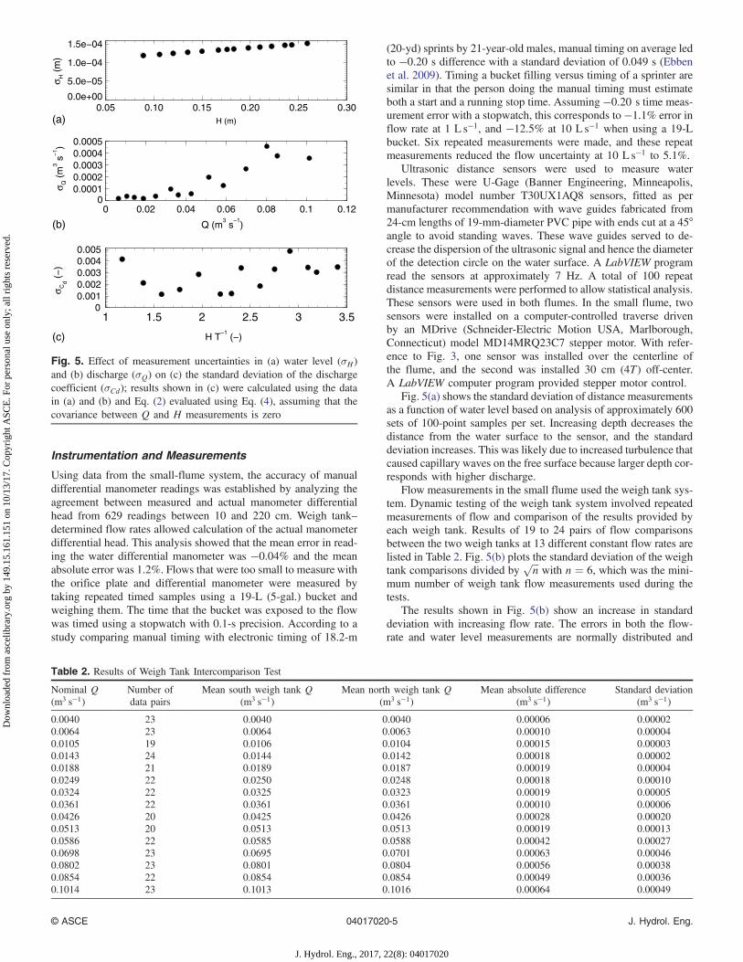
Fig. 5(a) shows the standard deviation of distance measurementsas a function of water level based on analysis of approximately 600sets of 100-point samples per set. Increasing depth decreases thedistance from the water surface to the sensor, and the standarddeviation increases. This was likely due to increased turbulence thatcaused capillary waves on the free surface because larger depth cor-responds with higher discharge.

Flow measurements in the small flume used the weigh tank sys-tem. Dynamic testing of the weigh tank system involved repeatedmeasurements of flow and comparison of the results provided byeach weigh tank. Results of 19 to 24 pairs of flow comparisonsbetween the two weigh tanks at 13 different constant flow rates arelisted in Table 2. Fig. 5(b) plots the standard deviation of the weightank comparisons divided by

ffiffiffin

pwith n ¼ 6, which was the mini-

mum number of weigh tank flow measurements used during thetests.

The results shown in Fig. 5(b) show an increase in standarddeviation with increasing flow rate. The errors in both the flow-rate and water level measurements are normally distributed and

(a)

(b)

(c)

Fig. 5. Effect of measurement uncertainties in (a) water level (σH)and (b) discharge (σQ) on (c) the standard deviation of the dischargecoefficient (σCd); results shown in (c) were calculated using the datain (a) and (b) and Eq. (2) evaluated using Eq. (4), assuming that thecovariance between Q and H measurements is zero

Table 2. Results of Weigh Tank Intercomparison Test

Nominal Q(m3 s−1)

Number ofdata pairs

Mean south weigh tank Q(m3 s−1)

Mean north weigh tank Q(m3 s−1)

Mean absolute difference(m3 s−1)

Standard deviation(m3 s−1)

0.0040 23 0.0040 0.0040 0.00006 0.000020.0064 23 0.0064 0.0063 0.00010 0.000040.0105 19 0.0106 0.0104 0.00015 0.000030.0143 24 0.0144 0.0142 0.00018 0.000020.0188 21 0.0189 0.0187 0.00019 0.000040.0249 22 0.0250 0.0248 0.00018 0.000100.0324 22 0.0325 0.0323 0.00019 0.000050.0361 22 0.0361 0.0361 0.00010 0.000060.0426 20 0.0425 0.0426 0.00028 0.000200.0513 20 0.0513 0.0513 0.00019 0.000130.0586 22 0.0585 0.0588 0.00042 0.000270.0698 23 0.0695 0.0701 0.00063 0.000460.0802 23 0.0801 0.0804 0.00056 0.000380.0854 22 0.0854 0.0854 0.00049 0.000360.1014 23 0.1013 0.1016 0.00064 0.00049

© ASCE 04017020-5 J. Hydrol. Eng.

J. Hydrol. Eng., 2017, 22(8): 04017020

Dow

nloa

ded

from

asc

elib

rary

.org

by

149.

15.1

61.1

51 o

n 10

/13/

17. C

opyr

ight

ASC

E. F

or p

erso

nal u

se o

nly;

all

righ

ts r

eser

ved.

uncorrelated, so the transmission of error method was used toapproximate the total measurement system variance (Montgomeryet al. 2007) using Eq. (4)

σ2ðCdÞ ¼�∂Cd

∂Q�2

σ2ðQÞ þ� ∂Cd

∂Htotal

�2

σ2ðHtotalÞ ð4Þ

In the case of triangular weirs, Eq. (1) was manipulated to pro-duce the partial derivative terms for use in Eq. (4). The use ofEq. (4) assumes that there is no covariance between the ultrasonicwater level sensors and the weigh tank system. Fig. 5(c) shows theresult of the measurement system errors on the calculated dischargecoefficients.

The results shown in Fig. 5(c) indicate that system measurementerrors are a relatively minor component of the uncertainty in theCd values. Other potential measurement error sources include theinitial nonflowing water surface elevation when the water surfaceis equal with the weir invert and the kinetic energy correctionfactor, α.

Methods

With reference to Fig. 1, variables manipulated in this study includechannel slope (So ¼ 0, 1, 2, 3%), sedimentation condition (P ¼0.6Hmax, P ¼ 0), crest shape (ARS: m ¼ 8, Panama: m ¼ 4), weirangle (θ ¼ 120°, 140°), depth measurement location along thechannel (2 ≤ xT−1 ≤ 18, where x is the along-stream distance fromthe weir face), and lateral location from weir centerline (yT−1 ¼ 0,yT−1 ¼ 4). To avoid scale effects at smaller values of normalizedflow depth HT−1, two weir thicknesses, T, were used in this study:20.32 and 7.62 cm in two different flumes.

Using the crest thickness T as a fundamental length variable inFroude similarity theory for free-surface flows, these different crestthicknesses can be considered different scales. Field values of T forthese short-crested weirs range from 20.32 to 43 cm. Therefore, therange of scales tested varied from 1∶1 in the case of the Panama weircrest where T ¼ 20.32 cm in the field, to 1∶5.64 in the case of theARS weir crest with field thickness 43 cm when tested in the labo-ratory with T ¼ 7.62 cm. The use of a scale as near as possibleto 1∶1 helps to avoid scale effects due to dissimilarities in theReynolds number and momentum flux and pressure forces in themodel and prototype that can affect the character of flow at the weircrest for short-crested weirs.

Determination of No-Flow Water Surface Elevation

Accurately establishing the water level datum that represents theweir invert elevation as read by the ultrasonic distance trans-ducer(s) is extremely important. Errors less than 1 mm cause largeerrors in discharge coefficient, particularly at lower values ofHT−1.These errors are plotted in Fig. 6 for the test conditions in the smallflume. Fig. 6 shows that a 1-mm error in the initial no-flow watersurface elevation causes from 2% to almost 6% error in calculatedCd depending on HT−1.

Relying on visual identification of the no-flow water surfaceelevation upon drain down is not reliable because of surface tensioneffects in the weir invert. At the start of each day’s testing, a sur-veying level was used to survey the invert elevation of the weirbeing tested using a mechanics rule graduated at 0.4 mm as a sur-veying rod. At close distance this mechanic’s rule could be read to aprecision of 0.2 mm. If this precision represents the standard errorof this effect on the discharge coefficient, then its portion of theerror budget is less than 0.5% over the range of HT−1 tested.

If present, pea gravel was scooped away from the areas wherethe ultrasonic sensors made measurements to a depth of 1 to 2 cmso that the pea gravel did not interfere with the ultrasonic sensorcalibration. The hook gauge was set to the same elevation as theweir invert by again surveying using the mechanics rule within0.2-mm precision as the survey rod. The flume was then filled withenough water to start flow over the weir. The water supply wasshut off, and the flume drained using a drain valve until the hookgauge point became exposed. The drain valve was closed immedi-ately to establish the no-flow water surface elevation that was usedto calibrate the ultrasonic distance transducer zero elevation datum.In the case of the small flume, the data acquisition program wasrun, which collected data representing no-flow initial water surfaceelevations from the computer control traverse at all 22 measure-ment locations.

A similar protocol was established in tests with the large flume.The no-flow initial condition was established by surveying the weirinvert elevation and using that observation to set a hook gauge.Water was added to establish flow over the weir and drained usinga drain valve until exposure of the tip of the hook gage. TheLabVIEW data acquisition program was run to collect 100 watersurface elevation points over an approximately 14-s period with7-Hz sampling frequency. The average of these points representedthe no-flow zero water surface datum. These data were useful fordetecting leaks in the large flume because filtered ultrasonic dis-tance transducer measurements can reveal extremely small changesO(10 μm) in the water surface elevation. Continuous change inwater surface elevation after closing the drain indicated a leak.

Standard Test Methodology

In general, tests involved increasing flows throughout the day. Thedifferential manometer was used to establish the flow rate. In testsin the small flume, the weigh tank program was run continuously,producing a new flow-rate measurement approximately every3 min. When the flow rate reached an equilibrium, the LabVIEWdata acquisition program was run, sampling the centerline and30-cm off-centerline ultrasonic distance sensors at 7 Hz, collecting100 data points at each position. The computer then commandedthe linear traverse to move 15 cm upstream, and repeat the 100distance measurements. Eleven positions spaced 15 cm apart alongthe length of the flume were sampled, resulting in a total of 22water level measurement locations. The output of a day’s testsincluded ASCII files containing 100 water level measurements

1 2 3H T

−1

0

2

4

6

Abs

olut

e er

ror

in c

alcu

late

d C

d (%

)

0.1 mm 0.2 mm 0.5 mm 1.0 mm

Fig. 6. Effect of initial Q ¼ 0 water surface elevation measurementerror on calculated discharge coefficient in percent, over a range ofmeasured water surface elevations in the small flumewith T ¼ 7.62 cm

© ASCE 04017020-6 J. Hydrol. Eng.

J. Hydrol. Eng., 2017, 22(8): 04017020

Dow

nloa

ded

from

asc

elib

rary

.org

by

149.

15.1

61.1

51 o

n 10

/13/

17. C

opyr

ight

ASC

E. F

or p

erso

nal u

se o

nly;

all

righ

ts r

eser

ved.

at 22 locations for each of the 17 discharges tested, including theno-flow set.

Because flow measurements in the large flume depended uponeither timed volumetric or orifice flow–differential manometermeasurements, the ultrasonic water level sensor was used to deter-mine steady state. The LabVIEW program continuously plottedwater level in an on-screen graph versus time. After an increasein flow rate, the water level was observed until it remained un-changed for at least 2 min. At that time, a LabVIEW program wasactivated to read the one ultrasonic distance sensor at 7-Hz fre-quency to collect 100 data points. Those data points were writtento a file. The differential manometer was read before and after therunning of the distance logging program. These two readings wereentered into the spreadsheet. If either the flow or the water surfaceelevation experienced a noticeable change, then the measurementwas repeated. In later tests, a hook gauge reading was taken beforeand after running the LabVIEW program as an independent checkof steady-state conditions.

Analysis of Water Surface Elevation Measurements

A computer program was written that performed several key dataprocessing functions. First, acting on the 100 repeat measurementsof water level, it performed outlier detection and normality testingusing the Shapiro and Wilk (1965) test, discarding extreme outliersto ensure data normality with p ¼ 0.05, then calculating the firstfour moments of the distribution. Occasionally some sequences of0.0 distance measurement occurred in the output due to latency andbuffer synchronization errors. In no case were fewer than 20 valuesused in computation of statistics, and most often fewer than 10 out-liers were removed. Second, this program used the no-flow waterlevel readings to calibrate the zero-head datum for each ultrasonicsensor position and each flow. This datum was subtracted fromwater level measurements during each flow to calculate the velocityand total head Htotal. Finally, the program calculated the dischargecoefficients, Cd, and wrote output files of Cd versus Q for eachmeasurement position, for velocity-head corrected (Htotal) and un-corrected (h) measurements.

Approach flow velocity profiles were not measured. Mefford(1979) performed multiple measurements of α in several differentchannel shapes above triangular short-crested weirs in a 2.44-m-wide flume. Chow (1959) recommended α values between 1.03and 1.36, while Brakensiek et al. (1979) assumed α ¼ 1.33.Because of similarities with Mefford’s experimental geometry

and flows, Mefford’s (1979) average measured value α ¼ 1.115was applied in the present study.

Repeatability of experiments was challenging because of errorssuch as those related to initial water surface elevation measure-ments or other unpredictable factors. Repeat experiments allowedquantification of the uncertainty of the Cd values. The number ofrepeat experiments varied from four to nine depending on test con-dition. The 95% confidence intervals (p ¼ 0.05) were computedusing the Student’s t distribution from the results of n independentCd measurements with standard deviation s as

C̄d � t0.05;n−1�

sffiffiffin

p�

ð5Þ

Simulation of Sedimentation

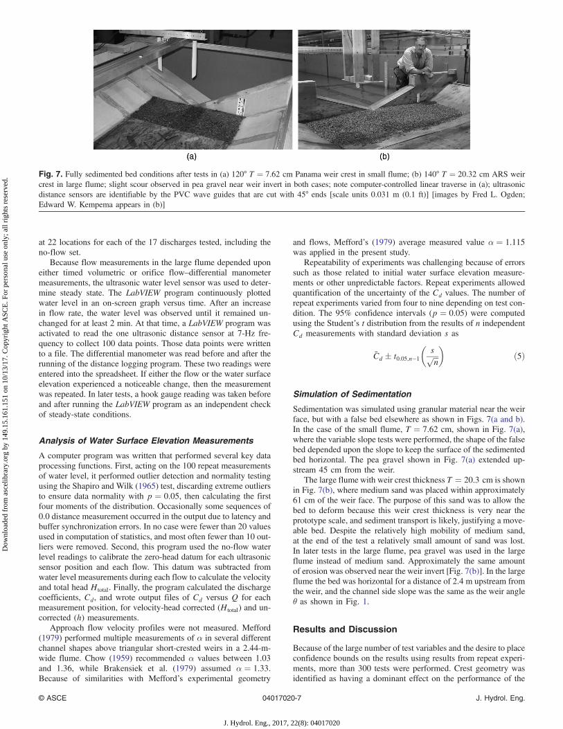
Sedimentation was simulated using granular material near the weirface, but with a false bed elsewhere as shown in Figs. 7(a and b).In the case of the small flume, T ¼ 7.62 cm, shown in Fig. 7(a),where the variable slope tests were performed, the shape of the falsebed depended upon the slope to keep the surface of the sedimentedbed horizontal. The pea gravel shown in Fig. 7(a) extended up-stream 45 cm from the weir.

The large flume with weir crest thickness T ¼ 20.3 cm is shownin Fig. 7(b), where medium sand was placed within approximately61 cm of the weir face. The purpose of this sand was to allow thebed to deform because this weir crest thickness is very near theprototype scale, and sediment transport is likely, justifying a move-able bed. Despite the relatively high mobility of medium sand,at the end of the test a relatively small amount of sand was lost.In later tests in the large flume, pea gravel was used in the largeflume instead of medium sand. Approximately the same amountof erosion was observed near the weir invert [Fig. 7(b)]. In the largeflume the bed was horizontal for a distance of 2.4 m upstream fromthe weir, and the channel side slope was the same as the weir angleθ as shown in Fig. 1.

Results and Discussion

Because of the large number of test variables and the desire to placeconfidence bounds on the results using results from repeat experi-ments, more than 300 tests were performed. Crest geometry wasidentified as having a dominant effect on the performance of the

Fig. 7. Fully sedimented bed conditions after tests in (a) 120° T ¼ 7.62 cm Panama weir crest in small flume; (b) 140° T ¼ 20.32 cm ARS weircrest in large flume; slight scour observed in pea gravel near weir invert in both cases; note computer-controlled linear traverse in (a); ultrasonicdistance sensors are identifiable by the PVC wave guides that are cut with 45° ends [scale units 0.031 m (0.1 ft)] [images by Fred L. Ogden;Edward W. Kempema appears in (b)]

© ASCE 04017020-7 J. Hydrol. Eng.

J. Hydrol. Eng., 2017, 22(8): 04017020

Dow

nloa

ded

from

asc

elib

rary

.org

by

149.

15.1

61.1

51 o

n 10

/13/

17. C

opyr

ight

ASC

E. F

or p

erso

nal u

se o

nly;

all

righ

ts r

eser

ved.

weirs. For this reason the results are presented separately for thetwo weir crest geometries tested. With reference to Fig. 1, the ARScrest has m ¼ 8, while the Panama crest has m ¼ 4.

ARS Weir Crest

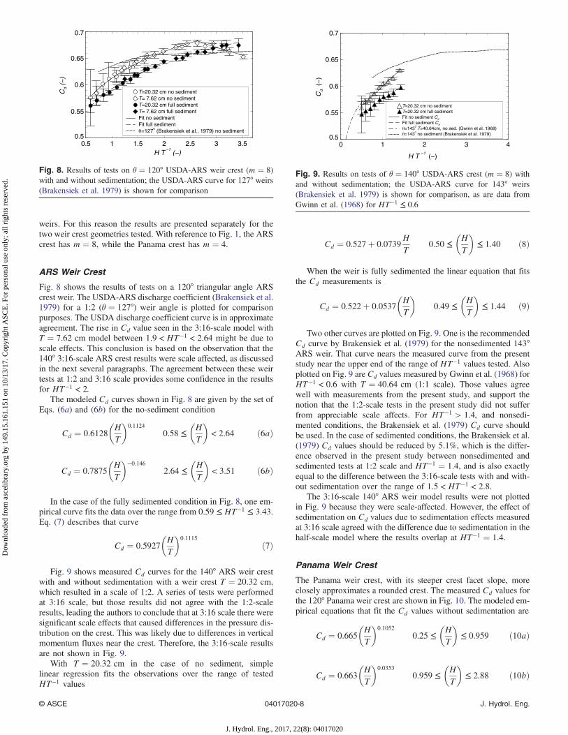
Fig. 8 shows the results of tests on a 120° triangular angle ARScrest weir. The USDA-ARS discharge coefficient (Brakensiek et al.1979) for a 1∶2 (θ ¼ 127°) weir angle is plotted for comparisonpurposes. The USDA discharge coefficient curve is in approximateagreement. The rise in Cd value seen in the 3∶16-scale model withT ¼ 7.62 cm model between 1.9 < HT−1 < 2.64 might be due toscale effects. This conclusion is based on the observation that the140° 3∶16-scale ARS crest results were scale affected, as discussedin the next several paragraphs. The agreement between these weirtests at 1∶2 and 3∶16 scale provides some confidence in the resultsfor HT−1 < 2.

The modeled Cd curves shown in Fig. 8 are given by the set ofEqs. (6a) and (6b) for the no-sediment condition

Cd ¼ 0.6128

�HT

�0.1124

0.58 ≤�HT

�< 2.64 ð6aÞ

Cd ¼ 0.7875

�HT

�−0.1462.64 ≤

�HT

�< 3.51 ð6bÞ

In the case of the fully sedimented condition in Fig. 8, one em-pirical curve fits the data over the range from 0.59 ≤ HT−1 ≤ 3.43.Eq. (7) describes that curve

Cd ¼ 0.5927

�HT

�0.1115

ð7Þ

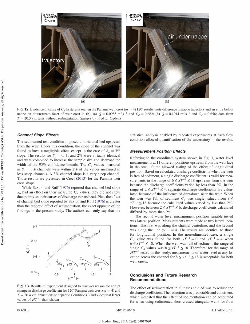
Fig. 9 shows measured Cd curves for the 140° ARS weir crestwith and without sedimentation with a weir crest T ¼ 20.32 cm,which resulted in a scale of 1∶2. A series of tests were performedat 3∶16 scale, but those results did not agree with the 1∶2-scaleresults, leading the authors to conclude that at 3∶16 scale there weresignificant scale effects that caused differences in the pressure dis-tribution on the crest. This was likely due to differences in verticalmomentum fluxes near the crest. Therefore, the 3∶16-scale resultsare not shown in Fig. 9.

With T ¼ 20.32 cm in the case of no sediment, simplelinear regression fits the observations over the range of testedHT−1 values

Cd ¼ 0.527þ 0.0739HT

0.50 ≤�HT

�≤ 1.40 ð8Þ

When the weir is fully sedimented the linear equation that fitsthe Cd measurements is

Cd ¼ 0.522þ 0.0537

�HT

�0.49 ≤

�HT

�≤ 1.44 ð9Þ

Two other curves are plotted on Fig. 9. One is the recommendedCd curve by Brakensiek et al. (1979) for the nonsedimented 143°ARS weir. That curve nears the measured curve from the presentstudy near the upper end of the range of HT−1 values tested. Alsoplotted on Fig. 9 are Cd values measured by Gwinn et al. (1968) forHT−1 < 0.6 with T ¼ 40.64 cm (1∶1 scale). Those values agreewell with measurements from the present study, and support thenotion that the 1∶2-scale tests in the present study did not sufferfrom appreciable scale affects. For HT−1 > 1.4, and nonsedi-mented conditions, the Brakensiek et al. (1979) Cd curve shouldbe used. In the case of sedimented conditions, the Brakensiek et al.(1979) Cd values should be reduced by 5.1%, which is the differ-ence observed in the present study between nonsedimented andsedimented tests at 1∶2 scale and HT−1 ¼ 1.4, and is also exactlyequal to the difference between the 3∶16-scale tests with and with-out sedimentation over the range of 1.5 < HT−1 < 2.8.

The 3∶16-scale 140° ARS weir model results were not plottedin Fig. 9 because they were scale-affected. However, the effect ofsedimentation on Cd values due to sedimentation effects measuredat 3∶16 scale agreed with the difference due to sedimentation in thehalf-scale model where the results overlap at HT−1 ¼ 1.4.

Panama Weir Crest

The Panama weir crest, with its steeper crest facet slope, moreclosely approximates a rounded crest. The measured Cd values forthe 120° Panama weir crest are shown in Fig. 10. The modeled em-pirical equations that fit the Cd values without sedimentation are

Cd ¼ 0.665

�HT

�0.1052

0.25 ≤�HT

�≤ 0.959 ð10aÞ

Cd ¼ 0.663

�HT

�0.0353

0.959 ≤�HT

�≤ 2.88 ð10bÞ

0.5 1 1.5 2 2.5 3 3.5H T

−1 (−)

0.5

0.55

0.6

0.65

0.7

Cd

(−)

T=20.32 cm no sedimentT= 7.62 cm no sedimentT=20.32 cm full sedimentT= 7.62 cm full sedimentFit no sedimentFit full sediment=127

o (Brakensiek et al., 1979) no sediment

Fig. 8. Results of tests on θ ¼ 120° USDA-ARS weir crest (m ¼ 8)with and without sedimentation; the USDA-ARS curve for 127° weirs(Brakensiek et al. 1979) is shown for comparison

0 1 2 3 4

H T −1

(−)

0.5

0.55

0.6

0.65

0.7

Cd

(−

)

T=20.32 cm no sedimentT=20.32 cm full sedimentFit no sediment Cd

Fit full sediment Cd

=1430 T=40.64cm, no sed. (Gwinn et al. 1968)=143o no sediment (Brakensiek et al. 1979)

Fig. 9. Results on tests of θ ¼ 140° USDA-ARS crest (m ¼ 8) withand without sedimentation; the USDA-ARS curve for 143° weirs(Brakensiek et al. 1979) is shown for comparison, as are data fromGwinn et al. (1968) for HT−1 ≤ 0.6

© ASCE 04017020-8 J. Hydrol. Eng.

J. Hydrol. Eng., 2017, 22(8): 04017020

Dow

nloa

ded

from

asc

elib

rary

.org

by

149.

15.1

61.1

51 o

n 10

/13/

17. C

opyr

ight

ASC

E. F

or p

erso

nal u

se o

nly;

all

righ

ts r

eser

ved.

Cd ¼ 0.707

�HT

�−0.02552.88 ≤

�HT

�≤ 3.43 ð10cÞ

When the 120° Panama weir is fully sedimented, the empiricalfit equations that fit the Cd measurements are

Cd ¼ 0.655

�HT

�0.0935

0.25 ≤�HT

�≤ 0.814 ð11aÞ

Cd ¼ 0.647

�HT

�0.0325

0.814 ≤�HT

�≤ 2.72 ð11bÞ

Cd ¼ 0.681

�HT

�−0.01952.72 ≤

�HT

�≤ 3.43 ð11cÞ

The Cd values shown in Fig. 10 exhibit a discontinuity nearHT−1 ¼ 1.3. This discontinuity is due to a change in flow regimeand is discussed subsequently.

Fig. 11 shows the measured Cd values for the 140° Panama weircrest. In the nonsedimented case, the Cd values are empirically fitby two power-law relations for the range of HT−1 values tested

Cd ¼ 0.612

�HT

�0.1159

0.72 ≤�HT

�≤ 2.253 ð12aÞ

Cd ¼ 0.674

�HT

�−0.00172.253 ≤

�HT

�≤ 2.87 ð12bÞ

The fully sedimented 140° Panama weir crest is fit by a singlepower-law equation over the range of HT−1 values tested

Cd ¼ 0.571

�HT

�0.1332

0.74 ≤�HT

�≤ 2.85 ð13Þ

Also plotted on Fig. 11 is the Cd relation suggested byBrakensiek et al. (1979) for the 143° ARS weir crest withoutsedimentation. Coincidentally, it agrees reasonably well with the140° Panama weir crest Cd values measured without sedimentation.

Crest-Shape Effects

In both the sedimented and nonsedimented cases, the 120° Panamaweir crest exhibited a sudden drop in discharge coefficient from0.682 to 0.658 when HT−1 reached and exceeded approximately

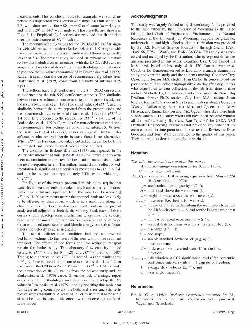
1.3. A series of measurements and observations involving smallincreases in discharge identified the cause of this sudden decreaseinCd in the case of increasing discharge. Repeat photography of thenappe showed differences in the trajectory and the aeration of thenappe occurring with a very small change in discharge as shownin Fig. 12.

Figs. 12(a and b) show two significant observed changes thatoccurred between Q ¼ 0.0985 m3 s−1 and Q ¼ 0.1014 m3 s−1.The first was that in Fig. 12(a), the nappe is in contact with thedownstream facet of the weir crest. In Fig. 12(b), there is evidenceof flow separation from the downsloping facet because air has in-vaded the space between that facet and the underside of the nappe.The second change observed is that the trajectory of the nappeis different. Comparing the trajectory of the nappe against thestructural timbers behind the nappe in Fig. 12(a) clearly showsthat the trajectory of the nappe is considerably steeper there thanin Fig. 12(b).

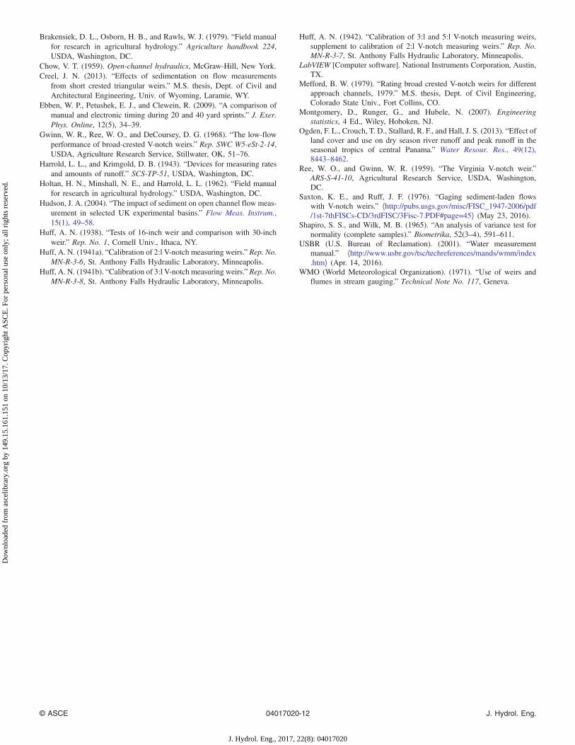
The effect of the condition shown in Fig. 12(a) is to create aregion of subatmospheric pressure on the downsloping facet of theweir crest. This allows the crest to have a slight siphon effect andacts to increase the discharge coefficient. The slight 0.0029 m3 s−1increase in flow corresponds to a sufficient increase in flow mo-mentum to allow the flow to separate from the downsloping crestfacet. The subsequent loss of suction results in a sudden decreasein Cd from 0.682 to 0.658, a decrease of 3.5%, as the data inFig. 13 show.

The geometry of the Panama and ARS weir crests offer threeopportunities for such transitions as shown on inset figures labeled1–4 on Fig. 13. There is a similar, albeit not as abrupt, decrease inCd seen in Fig. 8 for the 120° ARS weir for HT−1 slightly largerthan 2.5. This strong tendency to separate from the downslopingfacet of the weir crest creates a hysteresis in weir behavior, whichis undesirable. As shown in Fig. 13, the hysteresis occurs in theregion 1.1 < HT−1 < 1.4. As the results in Fig. 10 show, it is notparticularly pronounced compared with the remainder of the curve.When HT−1 > 1.4, this weir is well behaved with a near-constantCd value for both sedimented and nonsedimented conditions.

It is likely that the flow will transition from Condition 1 directlyto Condition 4 in the case of the ARS weir crest because of itsflatter crest design and more acute first facet angle (Fig. 12). Thatsaid, this transition was not seen in the T ¼ 7.62 cm tests of theARS weir crest that are not reported because of scale effects,and the failure to see this transition might be another scale effect.Furthermore, this transition was not seen in the T ¼ 20.32 cm tests,perhaps because of the limited flow rate in the apparatus.

0 0.5 1 1.5 2 2.5 3 3.5

H T −1

(−)

0.55

0.6

0.65

0.7

Cd

(−)

T=20.32 cm no sedimentT=7.62 cm no sedimentT=20.32 cm full sedimentT=7.62 cm full sedimentFit no sedimentFit full sediment

Fig. 10. Results of tests on θ ¼ 120° Panama weir crest (m ¼ 4) withand without sedimentation

0.5 1 1.5 2 2.5 3

H T −1

(−)

0.5

0.55

0.6

0.65

0.7

Cd

(−)

T= 7.62 cm no sedimentT= 7.62 cm full sedimentFit no sedimentFit full sediment=143

o no sediment (Brakensiek et al.1979)

Fig. 11. Results of tests on θ ¼ 140° Panama weir crest (m ¼ 4) withand without sedimentation; the USDA-ARS curve for 143° weirs(Brakensiek et al. 1979) is shown for comparison

© ASCE 04017020-9 J. Hydrol. Eng.

J. Hydrol. Eng., 2017, 22(8): 04017020

Dow

nloa

ded

from

asc

elib

rary

.org

by

149.

15.1

61.1

51 o

n 10

/13/

17. C

opyr

ight

ASC

E. F

or p

erso

nal u

se o

nly;

all

righ

ts r

eser

ved.

Channel Slope Effects

The sedimented test condition imposed a horizontal bed upstreamfrom the weir. Under this condition, the slope of the channel wasfound to have a negligible effect except in the case of So ¼ 3%

slope. The results for So ¼ 0, 1, and 2% were virtually identicaland were combined to increase the sample size and decrease thewidth of the 95% confidence bounds. The Cd values measuredin So ¼ 3% channels were within 2% of the values measured inless steep channels. A 3% channel slope is a very steep channel.Those results are presented in Creel (2013) for the Panama weircrest shape.

While Saxton and Ruff (1976) reported that channel bed slopeSo had an effect on their measured Cd values, they did not showdata points on their curves of discharge versus head. Plus, the effectof channel bed slope reported by Saxton and Ruff (1976) is greaterthan the reported effect of sedimentation, the exact opposite of thefindings in the present study. The authors can only say that the

statistical analysis enabled by repeated experiments at each flowcondition allowed quantification of the uncertainty in the results.

Measurement Position Effects

Referring to the coordinate system shown in Fig. 3, water levelmeasurements at 11 different positions upstream from the weir facein the small flume allowed testing of the effect of longitudinalposition. Based on calculated discharge coefficients when the weiris free of sediment, a single discharge coefficient is valid for mea-surements in the range of 6 ≤ xT−1 ≤ 18 upstream from the weirbecause the discharge coefficients varied by less than 2%. In therange of 2 ≤ xT−1 ≤ 4, separate discharge coefficients are calcu-lated because of the influence of drawdown near the weir. Whenthe weir was full of sediment Cd was single valued from 8 ≤xT−1 ≤ 18 because the calculated values varied by less than 2%.However, between 2 ≤ xT−1 ≤ 6, discharge coefficients calculateddiffered by more than 2%.

The second water level measurement position variable testedwas lateral position. Measurements were made at two lateral loca-tions. The first was along the channel centerline, and the secondwas along the line yT−1 ¼ 4. The results are identical to thosefor longitudinal position. In the nonsedimented case, a singleCd value was found for both yT−1 ¼ 0 and yT−1 ¼ 4 when6 ≤ xT−1 ≤ 18. When the weir was full of sediment the range ofsingle Cd values was 8 ≤ xT−1 ≤ 18. Therefore, for the range ofHT−1 tested in this study, measurements of water level at any lo-cation across the channel for 8 ≤ xT−1 ≤ 18 is acceptable for bothweir crests.

Conclusions and Future ResearchRecommendations

The effect of sedimentation in all cases studied was to reduce thedischarge coefficient. The reduction was predictable and consistent,which indicated that the effect of sedimentation can be accountedfor when using sedimented short-crested triangular weirs for flow

Fig. 12. Evidence of cause of Cd hysteresis seen in the Panama weir crest (m ¼ 4) 120° results; note difference in nappe trajectory and air entry belownappe on downstream facet of weir crest in (b): (a) Q ¼ 0.0985 m3 s−1 and Cd ¼ 0.682; (b) Q ¼ 0.1014 m3 s−1 and Cd ¼ 0.658; data fromT ¼ 20.3 cm tests without sedimentation (images by Fred L. Ogden)

0 0.5 1 1.5 2H T

−1 (−)

0.55

0.6

0.65

0.7

Cd

(−)

1 2 3 4

1

1

2

2

1

Fig. 13. Results of experiment designed to discover reason for abruptchange in discharge coefficient for 120° Panama weir crest (m ¼ 4) andT ¼ 20.4 cm; transitions to separate Conditions 3 and 4 occur at largervalues of HT−1 than shown

© ASCE 04017020-10 J. Hydrol. Eng.

J. Hydrol. Eng., 2017, 22(8): 04017020

Dow

nloa

ded

from

asc

elib

rary

.org

by

149.

15.1

61.1

51 o

n 10

/13/

17. C

opyr

ight

ASC

E. F

or p

erso

nal u

se o

nly;

all

righ

ts r

eser

ved.

measurements. This conclusion holds for triangular weirs in chan-nels with a trapezoidal cross section with slope less than or equal to2%, with short crest of the ARS (m ¼ 8) or Panama (m ¼ 4) type,and with 120° or 140° weir angle θ. Those results are shown inFigs. 8–11. Empirical Cd functions are provided that fit the dataover the tested range of HT−1 values.

The recommended Cd values for the USDA-ARS 143° triangu-lar weir without sedimentation (Brakensiek et al. 1979) agree withthe values measured in the present study with differences generallyless than 5%. The present study included an exhaustive literaturereview that included communications with the USDA-ARS, and nosingle report was found describing the methodology and data usedto produce the Cd values recommended in Brakensiek et al. (1979).Rather, it seems that the curves of recommended Cd values fromBrakensiek et al. (1979) come from a variety of internal ARSreports.

The authors have high confidence in the T ¼ 20.32 cm results,as evidenced by the thin 95% confidence intervals. The similaritybetween the nonsedimented curve reported in the present study andthe results by Gwinn et al. (1968) for small values ofHT−1, and thesimilarity between the curve reported from the present study andthe recommended curve by Brakensiek et al. (1979) for HT−1 >1.4 both lend credence to the results. For HT−1 > 1.4, use of theBrakensiek et al. (1979) Cd values for nonsedimented conditionsis recommended. For sedimented conditions, subtract 5.1% fromthe Brakensiek et al. (1979) Cd values as suggested by the scale-affected results reported herein because there is no alternative.When HT−1 is less than 1.4, values published herein for both thesedimented and nonsedimented cases should be used.

The assertion in Brakensiek et al. (1979) and repeated in theWater Measurement Manual (USBR 2001) that errors due to sedi-ment accumulation are greatest for low heads is not consistent withthe results reported herein. The authors found that the effect of sed-imentation is significant and persists in most cases to HT−1 > 3.4,and can be as great as approximately 10% over a wide rangeof HT−1.

Finally, use of the results presented in this study require thatwater level measurements be made at any location across the crosssection, at a distance upstream from the weir face between 8 ≤xT−1 ≤ 18. Measurements nearer the channel bank are less likelyto be affected by drawdown, which is at a maximum along thechannel centerline. Because discharge coefficients in the presentstudy are all adjusted to include the velocity head, users of thesecurves should develop some mechanism to estimate the velocityhead in their channel at the water surface measurement point basedon an estimated cross section and kinetic energy correction factor,unless the velocity head is negligible.

The tested sedimentation condition included a horizontalbed full of sediment to the invert of the weir with no live sedimenttransport. The effects of bed forms and live sediment transportremain for further study. The laboratory flow capacity limitedtesting to HT−1 < 3.5 for θ ¼ 120° and HT−1 < 3 for θ ¼ 140°.Testing to higher values of HT−1 is needed. As the results showin Fig. 9, there is a need to perform tests at scales of at least 1∶2 forthe case of the USDA-ARS 140° weir for HT−1 > 1.44 to verifythe intersection of the Cd values from the present study and theBrakensiek et al. (1979) curve. Given the lack of a single reportdescribing the methodology and data used to develop the Cd

values in Brakensiek et al. (1979), a study revisiting that topic nearfull scale using contemporary methods and error analysis tech-niques seems warranted. A scale of 1∶1 or as near to it as possibleshould be used because scale effects were observed in the 3∶16-scale model.

Acknowledgments

This study was largely funded using discretionary funds providedto the first author by the University of Wyoming as the ClineDistinguished Chair of Engineering, Environment, and NaturalResources at the University of Wyoming. Support for graduate,undergraduate, and high school student participation was providedby the U.S. National Science Foundation through Grants EAR-1045166, EPS-1135483, and EAR-1360384. This study was con-ceived and managed by the first author, who is responsible for theanalysis presented in this paper. Coauthor Jesse Creel earned hisM.S. thesis based on his study of the 120° Panama weir crest.Coauthor Ed Kempema served as laboratory manager during thisstudy and kept the study and the students moving. Coauthor TreyCrouch and former M.S. student Juan Carlos Briceno showed thepatience to reliably collect high-quality data day after day. Otherswho contributed to data collection in the lab from time to timeinclude Michelle Ogden, former postdoctoral associate Nawa RajPradhan, former Ph.D. student Guy Litt, M.S. student JasonRegina, former M.S. student Nels Frazier, undergraduates Cornelus“Casey” Valkenburg, Samantha Marquard-Ogden, and DrewHerrera, and Emma Erikson and Fritz Ogden when they were highschool students. This study would not have been possible withoutall their effort. Sherry Hunt and Ron Tejral of the USDA-ARSHydraulic Engineering Research Unit provided key historical lit-erature to aid in interpretation of past results. Reviewers DaveGoodrich and Tony Wahl contributed to the quality of this paper.Their attention to details is greatly appreciated.

Notation

The following symbols are used in this paper:A = kinetic energy correction factor (Chow 1959);Cd = discharge coefficient;

C0, C1 = constants in USDA rating equations from Manual 224(Brakensiek et al. 1979);

g = acceleration due to gravity (LT−2);H = total head above the weir invert (L);h = height of water above the weir invert (L);

hmax = maximum flow height for weir (L);m = divisor of T used in describing the weir crest shape; for

the ARS weir crestm ¼ 8, and for the Panama weir crestm ¼ 4;

n = number of repeat experiments (n ≥ 4);P = vertical distance from weir invert to stream bed (L);Q = discharge (L3T−1);So = bed slope;s = sample standard deviation of (n ≥ 4) Cd

measurements;T = thickness of short-crested weir (L) in the flow

direction;t0.05;n−1 = t distribution at 0.05 significance level (95th percentile

confidence interval) with n − 1 degrees of freedom;V = average flow velocity (LT−1); andΘ = weir angle (radians).

References

Bos, M. G., ed. (1989). Discharge measurement structures, 3rd Ed.,International Institute for Land Reclamation and Improvement,Wageningen, Netherlands.

© ASCE 04017020-11 J. Hydrol. Eng.

J. Hydrol. Eng., 2017, 22(8): 04017020

Dow

nloa

ded

from

asc

elib

rary

.org

by

149.

15.1

61.1

51 o

n 10

/13/

17. C

opyr

ight

ASC

E. F

or p

erso

nal u

se o

nly;

all

righ

ts r

eser

ved.

Brakensiek, D. L., Osborn, H. B., and Rawls, W. J. (1979). “Field manualfor research in agricultural hydrology.” Agriculture handbook 224,USDA, Washington, DC.

Chow, V. T. (1959). Open-channel hydraulics, McGraw-Hill, New York.Creel, J. N. (2013). “Effects of sedimentation on flow measurements

from short crested triangular weirs.” M.S. thesis, Dept. of Civil andArchitectural Engineering, Univ. of Wyoming, Laramie, WY.

Ebben, W. P., Petushek, E. J., and Clewein, R. (2009). “A comparison ofmanual and electronic timing during 20 and 40 yard sprints.” J. Exer.Phys. Online, 12(5), 34–39.

Gwinn, W. R., Ree, W. O., and DeCoursey, D. G. (1968). “The low-flowperformance of broad-crested V-notch weirs.” Rep. SWC W5-eSt-2-14,USDA, Agriculture Research Service, Stillwater, OK, 51–76.

Harrold, L. L., and Krimgold, D. B. (1943). “Devices for measuring ratesand amounts of runoff.” SCS-TP-51, USDA, Washington, DC.

Holtan, H. N., Minshall, N. E., and Harrold, L. L. (1962). “Field manualfor research in agricultural hydrology.” USDA, Washington, DC.

Hudson, J. A. (2004). “The impact of sediment on open channel flow meas-urement in selected UK experimental basins.” Flow Meas. Instrum.,15(1), 49–58.

Huff, A. N. (1938). “Tests of 16-inch weir and comparison with 30-inchweir.” Rep. No. 1, Cornell Univ., Ithaca, NY.

Huff, A. N. (1941a). “Calibration of 2:l V-notch measuring weirs.” Rep. No.MN-R-3-6, St. Anthony Falls Hydraulic Laboratory, Minneapolis.

Huff, A. N. (1941b). “Calibration of 3:l V-notch measuring weirs.” Rep. No.MN-R-3-8, St. Anthony Falls Hydraulic Laboratory, Minneapolis.

Huff, A. N. (1942). “Calibration of 3:l and 5:l V-notch measuring weirs,supplement to calibration of 2:l V-notch measuring weirs.” Rep. No.MN-R-3-7, St. Anthony Falls Hydraulic Laboratory, Minneapolis.

LabVIEW [Computer software]. National Instruments Corporation, Austin,TX.

Mefford, B. W. (1979). “Rating broad crested V-notch weirs for differentapproach channels, 1979.” M.S. thesis, Dept. of Civil Engineering,Colorado State Univ., Fort Collins, CO.

Montgomery, D., Runger, G., and Hubele, N. (2007). Engineeringstatistics, 4 Ed., Wiley, Hoboken, NJ.

Ogden, F. L., Crouch, T. D., Stallard, R. F., and Hall, J. S. (2013). “Effect ofland cover and use on dry season river runoff and peak runoff in theseasonal tropics of central Panama.” Water Resour. Res., 49(12),8443–8462.

Ree, W. O., and Gwinn, W. R. (1959). “The Virginia V-notch weir.”ARS-S-41-10, Agricultural Research Service, USDA, Washington,DC.

Saxton, K. E., and Ruff, J. F. (1976). “Gaging sediment-laden flowswith V-notch weirs.” ⟨http://pubs.usgs.gov/misc/FISC_1947-2006/pdf/1st-7thFISCs-CD/3rdFISC/3Fisc-7.PDF#page=45⟩ (May 23, 2016).

Shapiro, S. S., and Wilk, M. B. (1965). “An analysis of variance test fornormality (complete samples).” Biometrika, 52(3–4), 591–611.

USBR (U.S. Bureau of Reclamation). (2001). “Water measurementmanual.” ⟨http://www.usbr.gov/tsc/techreferences/mands/wmm/index.htm⟩ (Apr. 14, 2016).

WMO (World Meteorological Organization). (1971). “Use of weirs andflumes in stream gauging.” Technical Note No. 117, Geneva.

© ASCE 04017020-12 J. Hydrol. Eng.

J. Hydrol. Eng., 2017, 22(8): 04017020

Dow

nloa

ded

from

asc

elib

rary

.org

by

149.

15.1

61.1

51 o

n 10

/13/

17. C

opyr

ight

ASC

E. F

or p

erso

nal u

se o

nly;

all

righ

ts r

eser

ved.