Seg3D Tutorial

Seg3D 2.1 Documentation

Center for Integrative Biomedical ComputingScientific Computing & Imaging Institute

University of Utah

Seg3D software download:

http://software.sci.utah.edu

Center for Integrative Biomedical Computing:

http://www.sci.utah.edu/cibc

This project was supported by grants from the National Center for Research Resources(5P41RR012553-14) and the National Institute of General Medical Sciences

(8 P41 GM103545-14) from the National Institutes of Health.

Author(s):Jeroen Stinstra, Josh Blauer, Jess Tate, Brett Burton, Ahrash Poursaid

Contents

1 Overview 4

1.1 Software requirements . . . . . . . . . . . . . . . . . . . . . . . . . . . . . . . 4

1.1.1 Seg3D 2.1 . . . . . . . . . . . . . . . . . . . . . . . . . . . . . . . . . 4

1.1.2 Required Datasets . . . . . . . . . . . . . . . . . . . . . . . . . . . . . 4

2 Basic Orientation 5

2.1 Starting Seg3D . . . . . . . . . . . . . . . . . . . . . . . . . . . . . . . . . . . 5

2.2 Loading A Dataset . . . . . . . . . . . . . . . . . . . . . . . . . . . . . . . . . 6

2.3 Navigation . . . . . . . . . . . . . . . . . . . . . . . . . . . . . . . . . . . . . . 8

2.4 Changing Views . . . . . . . . . . . . . . . . . . . . . . . . . . . . . . . . . . 9

2.5 Loading a second dataset . . . . . . . . . . . . . . . . . . . . . . . . . . . . . 9

3 Simple Operator Based Segmentation Strategies 11

3.1 DEMRI Dataset . . . . . . . . . . . . . . . . . . . . . . . . . . . . . . . . . . 11

3.2 Label Masks . . . . . . . . . . . . . . . . . . . . . . . . . . . . . . . . . . . . . 12

3.3 Paint Tool . . . . . . . . . . . . . . . . . . . . . . . . . . . . . . . . . . . . . . 12

3.4 Polyline Tool . . . . . . . . . . . . . . . . . . . . . . . . . . . . . . . . . . . . 14

3.5 Logical Operators . . . . . . . . . . . . . . . . . . . . . . . . . . . . . . . . . . 14

3.6 Isosurface . . . . . . . . . . . . . . . . . . . . . . . . . . . . . . . . . . . . . . 14

3.7 Mask Data . . . . . . . . . . . . . . . . . . . . . . . . . . . . . . . . . . . . . 16

3.8 Saving . . . . . . . . . . . . . . . . . . . . . . . . . . . . . . . . . . . . . . . . 16

4 Filters and Threshold Tool 18

4.1 Loading Angiogram . . . . . . . . . . . . . . . . . . . . . . . . . . . . . . . . 19

4.2 Filtering data . . . . . . . . . . . . . . . . . . . . . . . . . . . . . . . . . . . . 19

4.3 Threshold Tool . . . . . . . . . . . . . . . . . . . . . . . . . . . . . . . . . . . 20

4.4 Otsu Threshold . . . . . . . . . . . . . . . . . . . . . . . . . . . . . . . . . . . 21

4.5 Canny Edge Detection Filter . . . . . . . . . . . . . . . . . . . . . . . . . . . 22

4.5.1 Canny Edge Detection With Mean Filter . . . . . . . . . . . . . . . . 23

5 Speedline Tool 25

5.1 Speedline Tool Segmentation . . . . . . . . . . . . . . . . . . . . . . . . . . . 25

6 Segmenting a Brain Dataset 28

6.1 Loading Datasets . . . . . . . . . . . . . . . . . . . . . . . . . . . . . . . . . . 28

6.2 Neighborhood Connected . . . . . . . . . . . . . . . . . . . . . . . . . . . . . 29

2

6.3 Filtering MRI Data . . . . . . . . . . . . . . . . . . . . . . . . . . . . . . . . . 306.4 Masking out Brain . . . . . . . . . . . . . . . . . . . . . . . . . . . . . . . . . 316.5 Thresholding Gray and White Matter . . . . . . . . . . . . . . . . . . . . . . 33

7 Conclusion 35

CONTENTS 3

Chapter 1

Overview

This tutorial describes step by step instructions to segment Ascending and Descending Aorta in car-diac MRI and describes the segmentation of skull, gray and white matter in a head dataset.

1.1 Software requirements

1.1.1 Seg3D 2.1

Seg3D is distributed as a binary download for Linux, Windows, and OS X. Please visit theSCI software portal to download the latest Seg3D binary. Any version of 2.0 or higher willdo.

1.1.2 Required Datasets

This tutorial uses two datasets. The first one is a set of two 3D scans, one is an anatomicalMRI of the atria and the second one is a delayed enhanced MR image of the same region.Both images have been registered. The second data is a brain data set that contains apreoperative MR image of the brain and a post surgery CT image of a pediatric patient.

The datasets are available in the SCIRunData zip files. Please visit SCIRun Data todownload the datasets. The datasets for this tutorial are inside the Seg3D directory. Thedirect linked to the zipped SCIRun Datasets can be found here.

4 Chapter 1

Chapter 2

Basic Orientation

Scope: Navigating in Seg3D

2.1 Starting Seg3D

When you start Seg3D, you will be greeted by the welcome screen (Figure 2.1). As you willsee, you have some options: you may load a recent project from the list (likely to be empty),open a project that you have saved on your machine, start a new project, take a quick lookat a single segmentation or image file, or you may quit Seg3D if you have changed yourmind.

Seg3D handles your data mainly in the form of projects which are similar to those usedin other applications. A project consists of a group of files and with this set up, Seg3D is ableto track and save your data that you are working on, the settings that you are using, andthe tools and filters that you are using. This is very useful, especially as your segmentations

Figure 2.1. Seg3D welcome screen

CHAPTER 2. BASIC ORIENTATION 5

Figure 2.2. Loading a volume

become larger and more complicated. For now, we will begin by starting a new project.Once you choose to open a new project, you will be asked to choose a name and locationfor the project. Test 1 will do for a name and the default location will be a directory thatwas created during installation called Seg3D-Projects. You can use this directory to storefuture projects.

2.2 Loading A Dataset

In order to get a good feel for the Seg3D program, one needs to load a dataset. Pleaseopen up the file menu and select the Import Layer From Single File... menu item asindicated in figure 2.2. This opens up a file browser. Browse to the Heart DataSet directoryand select this one to load the DEMRI.NRRD file.

The layer importer widget will then appear (figure 2.3). This widget is for distinguishinghow the data from the file is read and the widget is especially needed when loading previ-ously saved label masks. For this dataset, choose the only available option, which is DataVolume. This will load the file as a gray scale image volume.

Note: we converted the datasets for this demo into the NRRD dataset format as it doesnot contain any patient information. For more information on NRRD filetypes, refer to theNRRD Format. Seg3D reads DICOM files as well and any image file format supported bythe Insight ToolKit, as well as Matlab files. For additional supported filetypes, view thefiletype drop-down menu that appears while browsing to open a file. The browser decideswhich fileformat to use based on the extension of the file.

Once the file has loaded one can see the data being displayed in the 3 slice views and the

6 Chapter 2

Figure 2.3. Chose type of data to load

Figure 2.4. The main Seg3D window

3D viewer. The layout of the Seg3D program is highlighted in figure 2.4. On the top leftone has a tool menu that will show the options of the currently loaded tool and is currentlyempty. On the right one can see the layer menu. Each layer in Seg3D is a separate volumeand the order in the Layer Editor depicts the order in which datasets are being shown. Inthe center one has the three orthogonal views and one 3D viewer and to the lower left onecan browse the position of the active dataset and sample the value.

Some tools require data to be represented in a histogram, which would be shown in thetool menu. The histogram shows pixel intensities in a cross section of the image, and thedata from the histograms is used for image filtering. The data in the histogram can berepresented in either a logarithmic or a linear format, with the linear format showing linearvalues, which often results in more dramatic intensity gradients, and the logarithmic format

CHAPTER 2. BASIC ORIENTATION 7

Figure 2.5. The keyboard shortcuts as found in the help menu

showing an alternative, with lower intensities receiving a greater emphasis.

2.3 Navigation

Note: These operations are based on a setup that involves a three-button mouse. For otherconfigurations, see Keyboard Shortcuts in the Help menu (figure 2.5).

Brightness Move the mouse up and down while pressing left mouse button (only when avolume layer is selected).

Contrast Move the mouse left and right while pressing left mouse button (only when avolume layer is selected).

Pan Volume Press shift and move volume while clicking left mouse button (Volume viewonly).

Zoom Move the mouse up and down while pressing the right mouse button (Volume viewonly).

Rotate Move the mouse while pressing the middle mouse button in the 3D viewer (Volumeview only).

Move slice orthogonal slices Move the mouse while pressing the middle mouse buttonin the 2D view windows. This will change the location of the two colored lines, whichrepresent the location of the two other slice windows.

8 Chapter 2

Move slice depth Use the mouse wheel to move to the next slice. Or use the up anddown arrow keys, or the < and > keys, to navigate through a slice.

Painting In painting mode the mouse wheel is the size of the brush, hence to move throughslices use the up and down arrow keys, or the < and > key.

Plane visibility Press space to switch off viewing the image and space again to switch iton (all views, masks remain visible).

Navigate through the data and rotate the 3D image.

2.4 Changing Views

To alter the views that are displayed in the window. Press on the Red, Green, or Blue tabat the top of each Viewer to show a different viewer. By clicking on the labels one loopsthrough the four main modes of each window.

In the Views menu one can further specify the layout of the views. One can choosefrom:

Only one viewer Just showing one window.

One and One Two viewers side by side.

One and Two Make one big viewer and two smaller ones.

One and Three The default

Two by Two Four views of equal size.

Two and Three Make two viewers big and three smaller.

Three and Three Make six viewers.

There is also an option for a full screen mode which will fill the entire computer screenwith the Seg3D window. The top menu will pop down when the cursor is moved to the topof the screen.

2.5 Loading a second dataset

Open the Import Layer From Single File... menu once more and now load the An-gio.NRRD dataset by choosing Data Volume. After loading this dataset, two datasets arepresent in the menu on the right. You can see that because the data sets are in a differentgroup, i.e., they each have an orange header, the volumes are slightly different. By clickingon the i button for each volume you can see that the origins are slightly different. Youmay correct this using the Transform tool. With this tool you can change the origin ofone volume to match the other. The corrected volume will then join the other into a singlegroup. This step is not needed for the purposes of this tutorial, but tools and filters thatuse two layers as inputs cannot use layers of different groups.

Press on the eye to show which layer is visible. As volume layers are full data layers theycompletely clutter the underlying image. Switch on the visibility (using the eye) of both

CHAPTER 2. BASIC ORIENTATION 9

layers and toggle the visibility of the top most layer. The top most is the one found on topof the menu. The blue highlight set the selected layer. Select the top layer and press spaceand press space again (put the cursor in the Viewer Window). This option can be used toquickly view the difference between layers.

10 Chapter 2

Chapter 3

Simple Operator Based SegmentationStrategies

Scope: Paint Tool - Polyline Tool - Logical Operators - Creating Isosurfaces - Masking Data - SavingData - Morphological Filters

3.1 DEMRI Dataset

In this section we will use the paint and polyline tools to segment a simple structure, theaorta, from the DEMRI dataset. Delayed enhancement MRI (DEMRI) makes use of the

Figure 3.1. Painting the lumen of the descending aorta.

CHAPTER 3. SIMPLE OPERATOR BASED SEGMENTATION STRATEGIES 11

contrast enhancement that gadolinium (Gd) provides in MR imaging. In this scan Gd wasinjected via IV into the patient’s venous system. As the Gd washes through the system itenters and exits tissues at variable rates. In this case, 15 minutes after administration, theGd has washed into and out of most tissue. Enhanced tissues that continue to sequesterGd are assumed to have disrupted, or altered vascular perfusion. This method has be usedto detect cardiac ischemia, infarct, and scarring. This particular DEMRI dataset was usedto evaluate post-operative scarring in the left atrium. To get started, we will be looking atthe ascending and descending aorta.

3.2 Label Masks

Seg3D has two types of layers that can operated on by different tools and filters. These arevolume and label masks. Volumes are image data that has been loaded in, or produced byone of the filters. The DEMRI and Angio datasets loaded in the first section are volumes,and appear left aligned on the Layer Menu. If you select the + button below either of thesevolumes a new layer with the name ’Mask Layer’ appears indented above the volume. Thisis a label mask, and you may rename it anytime by clicking on the name of the layer. Thelabel mask displays the segmented regions of interest as a colored opaque layer. When usingany tool or feature it is important to know whether it operates on a volume, label mask, orboth.

3.3 Paint Tool

The paint and polyline tools allow the user to directly select regions of interest for segmen-tation. The paint tool presents as a circle icon of adjustable radius that can select regions ofinterest by holding down the left mouse button and moving the icon over the desired object.

Begin by selecting Paint Brush under Tools on the menu bar. When the circular iconappears, experiment with the tool by moving it over the three orthogonal image planes. Youwill notice that the icon is elliptical over the Coronal and Sagittal planes and is circular overthe Axial plane. Click on the i button under DEMRI on the Layer Menu and informationabout the volume will open. Next to Spacing is listed the voxel dimensions (0.62, 0.62,2.5). With respect to the Axial plane this means the slice thickness is nearly 4X the sizeof X-Y spacing. When using other features in Seg3D it is important to remember that theanisotropy of your data is preserved.

Prepare to segment by clicking on the + widget under DEMRI on the Layer Menu tocreate a label mask. Begin segmentation of the aorta by navigating the Paint icon over theDescending Aorta on the axial plane. Adjust the diameter of the tool with the scrollwheel, or by holding the right mouse button until it just fills the lumen of the aorta. Onceyou have positioned and sized the icon click the left mouse button. The circle icon shouldthen fill with the same color of the selected label mask. Proceed to the next few slicespainting the lumen of each one (Figure 3.1). Next, create a new label mask, and expandthe diameter of the Paint icon so it encircles the outer diameter, or superficial surface of theaorta. Now paint the superficial surface of the same slices. It is possible to erase paintingon the label mask by holding the right mouse button and moving the icon over the regionto be erased.

12 Chapter 3

Figure 3.2. Polyline for masking the lumen of the ascending aorta.

Figure 3.3. Polyline for masking the superficial surface of the ascending aorta.

CHAPTER 3. SIMPLE OPERATOR BASED SEGMENTATION STRATEGIES 13

3.4 Polyline Tool

The Polyline Tool may be better suited for segmentation of complex shapes. The polylinetool is operated by selecting points, with the left mouse button, around the perimeter ofthe region of interest. Each point added is connected to the point before it and to the firstpoint selected making a closed polygon. Both tools display the selected regions of interestin label masks.

Open the Polyline Tool under the Tools menu on the menu bar. Without changing thelabel mask, begin clicking points around the superficial surface of the Ascending Aorta(Figure 3.3). If you are not satisfied with the location of a point you can move it by movingyour cursor over the point, when the cursor turns into a had or a thicker cross, you may movethe point by left clicking on it and dragging it to the desired location. Or, you can simplydelete the point by right clicking on the point when when the cursor changes. The polylinetool will automatically try to place the point in the order that completes the smoothestshape, so when your are outlining a concave shape, make a convex shape, then add morepoints to make it concave. Once you have traced the superficial surface all the way aroundclick fill on the Tool Menu, or simply press F on the keyboard. The region surrounded bythe polyline should fill with the color of the selected label mask. Navigate to the next slice,and notice that the polyline does not disappear. If the polyline still matches the region ofinterest, simply hit F. To adjust the polyline hold shift cand left click on one point and dragto move the entire polyline, or move individual points as described before. If you want tostart over hit Clear Polyline button in the tool options on the left. It is also possible to eraseregions of the label mask with the Polyline tool by creating a polyline around the region tobe erased and selecting erase on the Tool Menu. After creating the superficial surface labelmasks hide the masks by clicking on the eye widget, select the lumen label mask, and usethe Polyline tool to create lumen masks on the Ascending Aorta (Figure 3.2).

3.5 Logical Operators

Once you have masked the lumen and superficial surface of both the ascending and de-scending aorta we can use logical operators to mask the real region of interest, the aortawall. Under Mask Filters on the menu bar, select Boolean Xor. Highlight either of the labelmasks. You will notice that the name of the highlighted filter will appear in the target layerfield. You can change this by unchecking the ‘Always use active layer’ option. Choose theother label mask in the Mask Layer option by selecting it from the list of eligible layers, orby holding down shift and clicking on the face color image of desired layer and dragging itto the option list. Click on the Run Filter button, this will create a new label mask thatonly covers the aorta wall (Figures 3.4). The resulting layer is shown in Figure 3.5. Noticethere is an option called Replace on the bottom of the tool menu. Most of the filters havethis option. It will replace the target layer with the result of the filter. This is very usefulwhen you do not need the unmodified layer after you run the filter.

3.6 Isosurface

To create a three dimensional isosurface of the Xor label mask, simple click the createisosurface icon (‘ISO ·’) for the layer. It may sometimes be necessary to delete an isosurface

14 Chapter 3

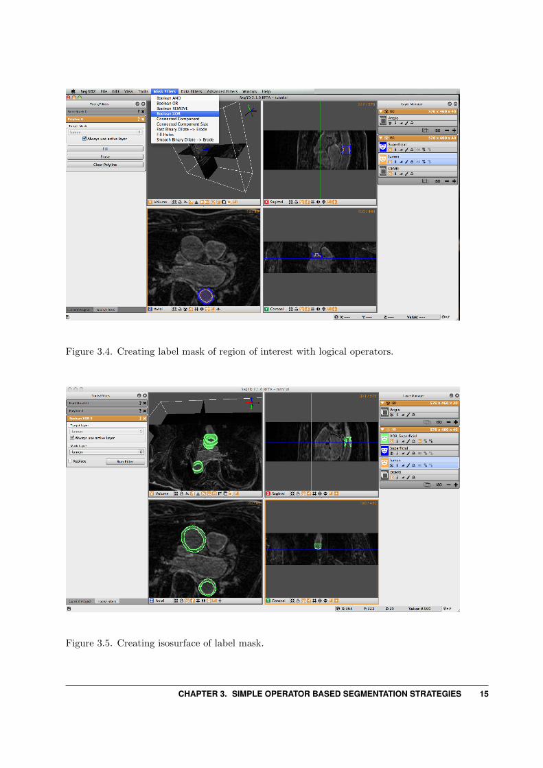
Figure 3.4. Creating label mask of region of interest with logical operators.

Figure 3.5. Creating isosurface of label mask.

CHAPTER 3. SIMPLE OPERATOR BASED SEGMENTATION STRATEGIES 15

Figure 3.6. Using label mask to extract data from volume.

that has already been created if you run a filter with the replace option (‘ISO ×’). OnceXor is the only layer highlighted, return to the Edit menu and select Isosurface CurrentLabel and click Start. Now the 3D View in the upper right corner should display the 3Disosurface (Figure 3.5). Navigate around the volume with the normal zoom and pan volumeshort keys. Holding the alt/option key and clicking (or middle click) on the volume willallow you to rotate the object. Experiment with the widgets in the bottom of the 3D viewerto turn on and off various elements of the display.

3.7 Mask Data

To extract the data covered by the label mask select the Mask Data option under theData Filters menu. Choose the label mask you want to use to extract data with and clickSet Label Mask in the Tools Menu. Select the Data layer you want to extract data from(DEMRI in this case), which should appear in the Target Layer field. Then choose the MaskLayer you wish to mask the data with (XOR Superficial) from the drop down menu or bydragging the layer to the field. Set the background value to the desired setting (min value),then click the Run Filter button. A new data layer will appear in the Layer Menu (calledMaskData DEMRI). This should show only the region of interest from the masked volume(Figure 3.6). You may need to toggle off the viewing of the mask layers to see the data.

3.8 Saving

At this point there are multiple options for saving the work that you have done. Underthe File menu are the options: Save Project, Save Project as ..., Export Segmentation, and

16 Chapter 3

Export Active Data Layer. There are hotkeys for these functions and many others thatcan be see by clicking the help menu then Keyboard Shortcuts. Save Project/Save Projectas ... will save the work that you done to this point in for later restoration. The ExportSegmentation option save the label masks that you have created. Export Active Data Layerwill save the image data selected in the Layer Menu. Individual mask and data layersmay be exported by right clicking on the layers and choosing Export Segmentation/Dataas... and then choosing the file type. As apparent, the export data types available are imagestacks (bitmap, png, tiff, dicom), matlab v7.3, and NRRD (see http://teem.sourceforge.net/nrrd/). The preferred data format for CIBC software is NRRD, and is required forusing BioMesh3D, a tetrahedral mesh generation software also developed by CIBC http:

//biomesh3d.com.

CHAPTER 3. SIMPLE OPERATOR BASED SEGMENTATION STRATEGIES 17

Chapter 4

Filters and Threshold Tool

Scope: Using Masks - Filtering Data

Figure 4.1. Angiogram

18 Chapter 4

Figure 4.2. Median and Gaussian filtered Angiogram

4.1 Loading Angiogram

The second cardiac dataset that is part of this example is the angiogram. For this part ofthe tutorial load the Angio.NRRD file. Use the Import Layer From Single File... menuin the File Menu to load this dataset. An example of this dataset is depicted in figure 4.1.

This dataset was previously registered to the DEMRI.NRRD dataset. As both datasetshave the sampling distance and coordinate system. One can use label mask from the DEMRIdataset in the Angio dataset and vice versa.

4.2 Filtering data

As we want to use the threshold tool on the Angiogram data to segment out the inner wallof the both ascending and descending aortas, the data noise in the MR image needs to besuppressed. In this example we use a Median Filter and Gaussian Blur to filter the data.

Open up the Median Filters from the Filters menu and select the Angio data layer asthe target. The radius indicates the number of the neighboring pixels that is used to derivethe median from. In this case the default setting of one will be sufficient. Run the filterand compare the results by pressing space to toggle on and off the selected layer, which inthis case should be the top most layer that was just generated if there are no mask layerspresent.

The second stage of filtering uses the Gaussian Blur from the Data Filters Menu.Again the default settings will do. Select the output from the median filter and run thisfilter. After filtering the data will look like the results depicted in figure 4.2.

CHAPTER 4. FILTERS AND THRESHOLD TOOL 19

Figure 4.3. Thresholding Angiogram while looking at DEMRI

4.3 Threshold Tool

To select the blood from the segmentation, use the Threshold Tool from the Tools menu.Once this tool has been opened, choose the filtered angio as the target and use the slidersto adjust the threshold values. In order to do this, switch off the visibility of both thefiltered Angio datasets as well as the original Angio dataset and make the DEMRI visible.This will allow you to interactively generate a segmentation of the blood using the DEMRIas a visual confirmation, and filtered angio data for the threshold. Once the segmentationlooks good press Create Threshold Layer in the Threshold Menu to generate the labellayer. (see figure 4.3) The threshold tool however segments both aortas and the left atrium.To select just one of the of the vessels, select the newly created label layer and then selectMask Data in the Data Filters Menu.

Now create a new layer by pressing on the + symbol in this layer. This will generate anew empty layer with the same dimensions. Now open up the Paint Brush in the ToolsMenu. Select the Mask Layer for theT

¯arget Layer in the Paint Brush Menu. Then under

Mask Constraint 1 select the Threshold Angio and start painting the Ascending Aorta.As a mask has been set the painting will be restricted to previously segmented blood. (seefigure 4.4)

Paint a couple of slices and then generate the isosurface of the vessel. Once you havecaptured the vessel to your satisfaction, you may export the segmentation as described inthe previous chapter.

20 Chapter 4

Figure 4.4. Painting a label while masking from another label

4.4 Otsu Threshold

Another thresholding tool available in the Data Filters menu is the Otsu Threshold. TheOtsu Threshold uses an image intensity histogram to determine adequate threshold levelsand segment the image based on the determined threshold levels. A demonstration of theOtsu Threshold will be done on the CT image that was taken on the 15 year old pediatricpatient.The file can be found in the SCIRun datasets (see section 1.1). We will be workingwith the CTbrain50.NRRD file found in the SCIRunData/Seg3D/Brain DataSet directory.

To use the Otsu Threshold, first select the Otsu Threshold tool from the Data Filtersmenu. The tools window will then show the information on the Otsu Threshold tool. Thetarget layer may be selected, and the number of thresholds can be selected, from zero to fourdifferent thresholding layers. Below the number of thresholds is the histogram representingthe intensities of the pixels of the image (figure 4.5). The menu box below the histogramallows the user to select whether they would like a logarithmic or a linear graph.

To use the Otsu Threshold tool on the brain CT image, select the tool and then choosethree as the number of thresholds. Select logarithmic for the display of the histogram, andrun the filter. The thresholded layers will appear in the layers view on the right. Thenumber of layers corresponds to the number of thresholds selected in the tool view. In thebrain data, the tool created different layers for dense matter like bone, other less densematter, and air (figure 4.6).

CHAPTER 4. FILTERS AND THRESHOLD TOOL 21

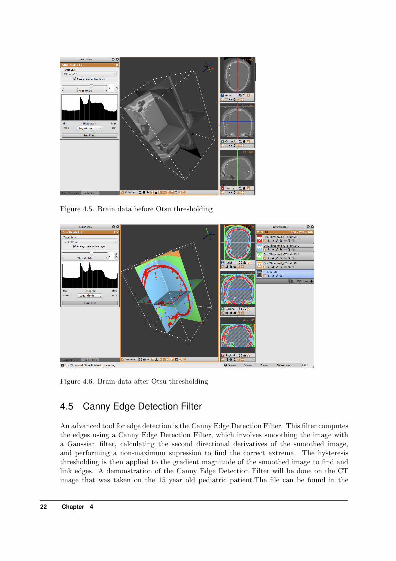
Figure 4.5. Brain data before Otsu thresholding

Figure 4.6. Brain data after Otsu thresholding

4.5 Canny Edge Detection Filter

An advanced tool for edge detection is the Canny Edge Detection Filter. This filter computesthe edges using a Canny Edge Detection Filter, which involves smoothing the image witha Gaussian filter, calculating the second directional derivatives of the smoothed image,and performing a non-maximum supression to find the correct extrema. The hysteresisthresholding is then applied to the gradient magnitude of the smoothed image to find andlink edges. A demonstration of the Canny Edge Detection Filter will be done on the CTimage that was taken on the 15 year old pediatric patient.The file can be found in the

22 Chapter 4

Figure 4.7. Brain data before Canny edge detection

SCIRun datasets (see section 1.1). We will be working with the CTbrain50.NRRD data file.To use the Canny edge detection filter on the volume, first select the Canny edge detec-

tion tool from the Advanced Filters menu. In the tools window, the Canny edge detectiontool will appear, allowing you to select the layer to run the filter on, as well as a distanceslider. The distance slider sets the variance for the Gaussian smoothing algorithm. Be-low, there is a slider to set the threshold for hysteresis thresholding to find and link edges.(figure 4.7).

The distance is the distance between edges, and the threshold is the pixel intensitythreshold for distinguishing edges. Select the distance as 4 and the threshold as 40. Whenthe layer, distance and threshold have been selected, run the filter to create a new layerwith the Canny edges displayed (figure 4.8). Note the detection of edges between densebone matter and less dense matter.

4.5.1 Canny Edge Detection With Mean Filter

The Canny edge detection filter may also be run by first applying a mean smoothing filterprior to applying the Canny edge detection filter.

The image in figure 4.9 had a mean filter applied to it with a radius of 6, followed by aCanny edge detection filter with a distance of 5 and a threshold of 30. Notice how smooththe image is prior to the application of the Canny filter.

CHAPTER 4. FILTERS AND THRESHOLD TOOL 23

Figure 4.8. Brain data after Canny edge detection

Figure 4.9. Canny edge detection with mean filter

24 Chapter 4

Chapter 5

Speedline Tool

Scope: Speedline Tool Segmentation

5.1 Speedline Tool Segmentation

In this example we will use the Speedline Tool (Also known as the Live Wire Tool) tosegment the Left Atrium. We start off with the Median Filtered Angiogram defined in theprevious chapter. This data will be the data on which we will using the speed tool.

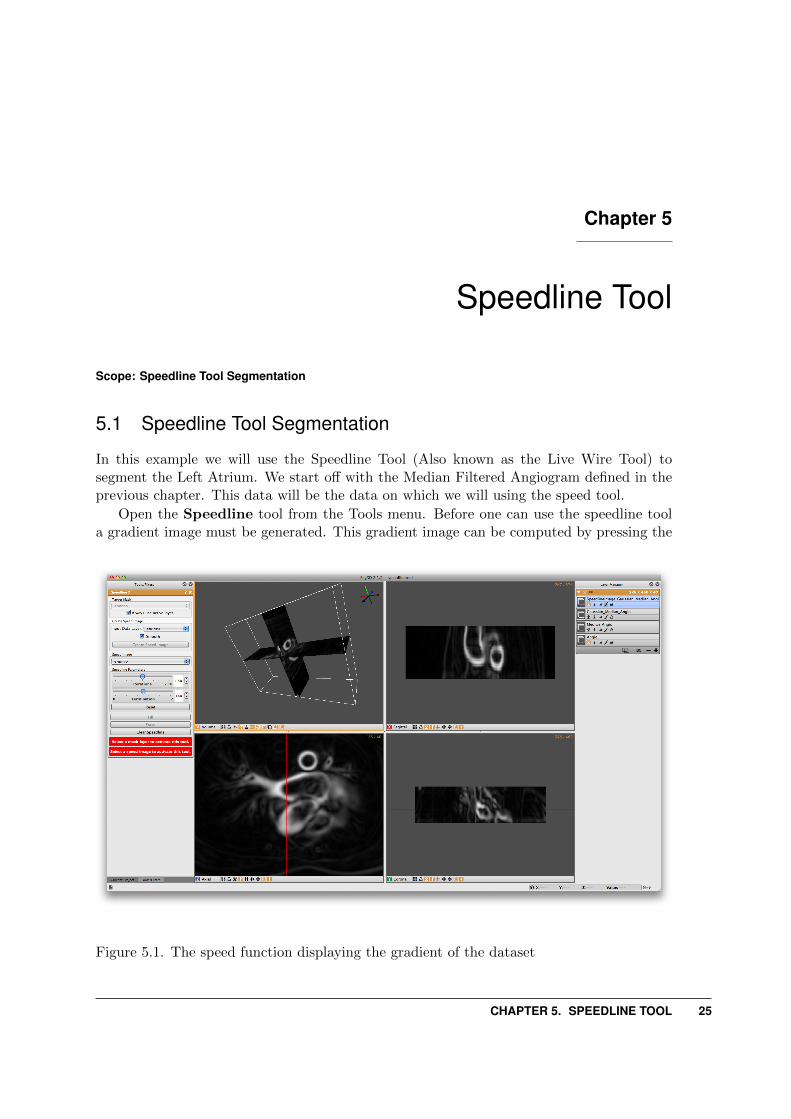
Open the Speedline tool from the Tools menu. Before one can use the speedline toola gradient image must be generated. This gradient image can be computed by pressing the

Figure 5.1. The speed function displaying the gradient of the dataset

CHAPTER 5. SPEEDLINE TOOL 25

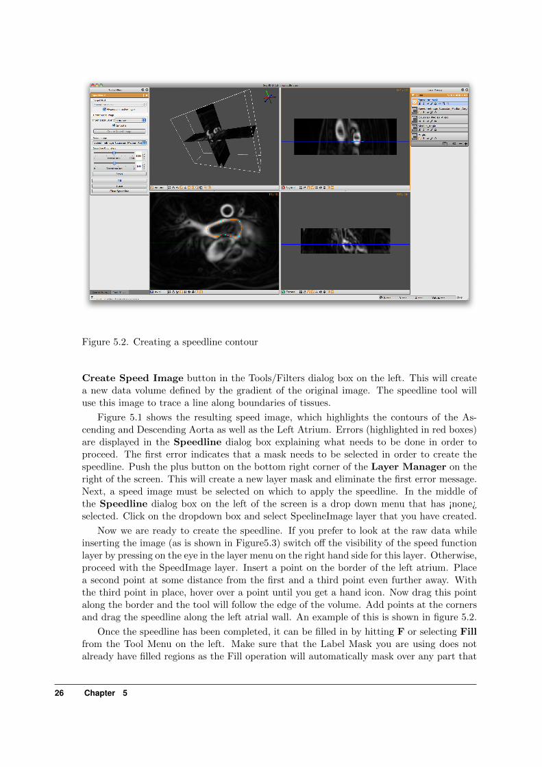
Figure 5.2. Creating a speedline contour

Create Speed Image button in the Tools/Filters dialog box on the left. This will createa new data volume defined by the gradient of the original image. The speedline tool willuse this image to trace a line along boundaries of tissues.

Figure 5.1 shows the resulting speed image, which highlights the contours of the As-cending and Descending Aorta as well as the Left Atrium. Errors (highlighted in red boxes)are displayed in the Speedline dialog box explaining what needs to be done in order toproceed. The first error indicates that a mask needs to be selected in order to create thespeedline. Push the plus button on the bottom right corner of the Layer Manager on theright of the screen. This will create a new layer mask and eliminate the first error message.Next, a speed image must be selected on which to apply the speedline. In the middle ofthe Speedline dialog box on the left of the screen is a drop down menu that has ¡none¿selected. Click on the dropdown box and select SpeelineImage layer that you have created.

Now we are ready to create the speedline. If you prefer to look at the raw data whileinserting the image (as is shown in Figure5.3) switch off the visibility of the speed functionlayer by pressing on the eye in the layer menu on the right hand side for this layer. Otherwise,proceed with the SpeedImage layer. Insert a point on the border of the left atrium. Placea second point at some distance from the first and a third point even further away. Withthe third point in place, hover over a point until you get a hand icon. Now drag this pointalong the border and the tool will follow the edge of the volume. Add points at the cornersand drag the speedline along the left atrial wall. An example of this is shown in figure 5.2.

Once the speedline has been completed, it can be filled in by hitting F or selecting Fillfrom the Tool Menu on the left. Make sure that the Label Mask you are using does notalready have filled regions as the Fill operation will automatically mask over any part that

26 Chapter 5

Figure 5.3. Filling in a speedline contour

is within the speedline.Now a segmentation is generated in one slice, proceed to the next slice by press < or >.

The speedtool will try to accommodate it’s shape to the new cross section. However, manualcorrections can be made by moving points around using the left or right mouse buttons anddragging point around, or by adding additional points by pressing the left mouse button inthe center of a segment. Press F again to fill in the segmentation. (see figure 5.3).

By doing this sequentially for many slices, one can quickly segment a section of a struc-ture. Once a portion of the structure has been segmented, press the ISO · button belowyour selected label mask in the Layer Manager window on the right to visualize the resultsin the 3D.

This concludes the cardiac part of this tutorial. The next chapter will highlight some ofthe tools using a head dataset.

CHAPTER 5. SPEEDLINE TOOL 27

Chapter 6

Segmenting a Brain Dataset

Scope: Neighborhood Connected - Thresholding using Points - Multiple Datasets -

6.1 Loading Datasets

This part of the tutorial deals with segmenting a head dataset. The data that will be usedis that of a 15 year old pediatric patient. This patient underwent surgery during whichelectrodes were implanted into the brain cavity. The image that we will be using are theMR image that was taken before the surgery and the CT image that was taken after. Notethat one can clearly see in the image where the electrodes were inserted.

Figure 6.1. Loading the brain dataset into Seg3D

28 Chapter 6

Figure 6.2. Selecting seed points for Neighborhood Connected filter

The final goal of this research is generate a patient specific model which can be used tofind focus of brain activity during a seizure. For this a full volumetric representation of thehead is needed. In this example we are extracting three tissues, namely the skull, the whitematter and the gray matter. The remaining scalp and CSF can be obtained similarly, butis outside the scope of this tutorial.

6.2 Neighborhood Connected

Browse the SCIRunData/Seg3D/Brain DataSet directory and load the following two files:CTbrain50.NRRD and MRI-brain50.NRRD. The first one is the post operative CT imageand the second one is the pre-surgery MR image. After loading the datasets the Seg3Dwindow should look like the one in figure 6.1.

Note that the data is not perfectly registered and that a part of the skull has been liftedto actually insert the electrode arrays.

To segment out the Skull we will be using the CT image. Select the CT image in theLayer Menu. Now from the Data Filters menu select the Neighborhood Connected filter.This filter needs seed points and finds every connected tissue of the same gray scale range.Hence placing seed points needs to be carefully. An example of this placement is given infigure 6.2.

Place the seed points with the left mouse button. While placing the seed points one canscroll to other slices. Each out of plain seed point will be shown less brightly. Place at least10 seed points or so and then run the filter on the CT image. Be sure to select that onebefore running the filter.

CHAPTER 6. SEGMENTING A BRAIN DATASET 29

Figure 6.3. Isosurfacing of Skull Segmentation

The result should look like the ones in figure 6.3. To help understanding the 3D natureof the data, select the newly created label layer and run the isosurface by clicking thecreate isosurface icon (‘ISO ·’) for the layer. This renders the isosurface of the currentsegmentation.

If parts of the skull are still missing, open up the Neighborhood Connected filteragain and add a few more seed points. Note that all the previous seed points are still thereto make it easier to add new points. To clear the seed points hit clear seed points in thefilter menu (if needed). To add additional regions just place seed points in those areas. Usethe isosurface rendering to check whether the skull is complete. Use the 3D view to seewhere the slices are and then put seed points where needed.

6.3 Filtering MRI Data

The MR data contents a good data set for segmenting the gray and white matter. HoweverMR images tend to have a bit of noise on them. Often running the data through the medianfilter will reduce the noise. Select the MR image in the Layer Menu and from the top menuselect the Median Filter from the Data Filters menu. Run this filter and compare it tothe previous MR image.

An easy way to do this is making all layers invisible, by clicking on the eye icons ofthe individual layers, and then make the original and the filtered MR image visible. Nowselect the top most image. Now the space bar will toggle between the two images. Navigatethrough the windows and look at the differences.

A second very useful filter for MR data is the Intensity Correction Filter from the

30 Chapter 6

Figure 6.4. Filtering the brain dataset

Advanced Filters menu. This filter takes a while to run but filters the intensity in the datathat have slight gradients due to the distance to the MR coils. The closer the image is to thelocation of the MR coil, the brighter the images generally are. This filter uses a polynomialmodel underneath to correct for this. We do this operation to make it easier to thresholdthe Gray and White Matter.

Apply this filter and again look at the differences. The resulting image is also given infigure 6.4.

6.4 Masking out Brain

To mask out brain, the easiest is to manually generate a mask and paint with a brush arough segmentation of the brain cavity. The goal of masking out the data is to be able tothreshold the white and gray matter inside the skull without picking up data from the scalp.

To jump start the process a segmentation is available in the dataset. This one wasgenerated by manually painting the slices. Load the label layer through the Import LayerFrom Single File... from the File menu. Choose the Brain.NRRD dataset. Then click onImport file as a Series of Masks: There are two of these options and either one is validbecause this data file has only one mask layer. After loading the dataset Seg3D should looklike the image depicted in figure 6.5.

Now use the Mask Data in the Data Filters menu to set the Brain segmentation asa mask. Select the MRI-brain50 for the Target Layer and Brain 1 for the Mask Layer.Then click on Run Filter. This will create an image where all the scalp and skull areremoved and only what is segmented is left as seen in figure 6.6. This mask will now be

CHAPTER 6. SEGMENTING A BRAIN DATASET 31

Figure 6.5. Load a pre-made rough segmentation of the brain

Figure 6.6. Mask brain data with hand painted segmentation

32 Chapter 6

Figure 6.7. Thresholding white matter using threshold range

used for segmenting the gray and white matter.

6.5 Thresholding Gray and White Matter

To segment the white matter, we select the Threshold Tool from the Tools menu. Beforeusing the tool make sure to turn off the Masking layer, by selecting ”The Eye” underneathBrain 1.

Now select the Masked Data Volume. With the Threshold Tool insert a few seedpoints in the white matter. The threshold tool will now segment all the points that arewithin the range of the seed points. Keep adding points until the white matter has beenmarked. (see figure 6.7). Once the segmentation is good enough press Create ThresholdLayer in the menu on the left and a new masking layer will be created.

Repeat the same procedure for the gray matter (see figure 6.8). Finally one can usethe boolean operators to subtract the white matter from the gray matter. Select BooleanAND in the Mask Filters menu. Select one of the masks as the Target Layer and theother as the Mask Layer and click on Run Filter.

CHAPTER 6. SEGMENTING A BRAIN DATASET 33

Figure 6.8. Thresholding grey matter using threshold range

34 Chapter 6

Chapter 7

Conclusion

This concludes the tutorial. Feel free to explore other structures in the head and make afull segmentation. Please explore the use of the other tools presented in this tutorial andincorporate them into your segmentation strategy if they are useful. Most of the tools andfilters not presented utilize a similar structure and are relatively self explanatory; try themout and use them in your project. Contact us at seg3d@sci.utah.edu with questions or bugreports and we will try to answer your questions.

CHAPTER 7. CONCLUSION 35