segmental concrete box girder bridge thermal analysis based...
TRANSCRIPT

SEGMENTAL CONCRETE BOX GIRDER BRIDGE THERMAL ANALYSIS BASED ON NEW TURKISH SOLAR ZONE MAP DEVELOPED TO ASSESS
TEMPERATURE GRADIENT LOADING
A THESIS SUBMITTED TO THE GRADUATE SCHOOL OF NATURAL AND APPLIED SCIENCES
OF MIDDLE EAST TECHNICAL UNIVERSITY
BY
ARZU İPEK YILMAZ
IN PARTIAL FULFILLMENT OF THE REQUIREMENTS FOR
THE DEGREE OF MASTER OF SCIENCE IN
CIVIL ENGINEERING
JANUARY 2015


Approval of the thesis:
SEGMENTAL CONCRETE BOX GIRDER BRIDGE THERMAL ANALYSIS BASED ON NEW TURKISH SOLAR ZONE MAP DEVELOPED TO ASSESS
TEMPERATURE GRADIENT LOADING
submitted by ARZU İPEK YILMAZ in partial fulfillment of the requirements for the degree of Master of Science in Civil Engineering Department, Middle East Technical University by, Prof. Dr.Gülbin Dural Ünver _________________ Dean, Graduate School of Natural and Applied Sciences Prof. Dr. Ahmet Cevdet Yalçıner _________________ Head of Department, Civil Engineering Assoc. Prof. Dr. Alp Caner _________________ Supervisor, Civil Engineering Dept., METU Examining Committee Members: Assoc. Prof. Dr.Ayşegül Askan Gündoğan _________________ Civil Engineering Dept., METU Assoc. Prof. Dr. Alp Caner _________________ Civil Engineering Dept., METU Assoc. Prof. Dr.Eray Baran _________________ Civil Engineering Dept., METU Assoc. Prof. Dr. Yalın Arıcı _________________ Civil Engineering Dept., METU Assist. Prof. Dr. Burcu Güneş _________________ Civil Engineering Dept., İTU
Date: ___30.01.2015_____

iv
I hereby declare that all information in this document has been obtained and presented in accordance with academic rules and ethical conduct. I also declare that, as required by these rules and conduct, I have fully cited and referenced all material and results that are not original to this work.
Name, Last Name : Arzu İpek Yılmaz Signature :

v
ABSTRACT
SEGMENTAL CONCRETE BOX GIRDER BRIDGE THERMAL ANALYSIS BASED ON NEW TURKISH SOLAR ZONE MAP DEVELOPED TO ASSESS
TEMPERATURE GRADIENT LOADING
Yılmaz, Arzu İpek
M.S., Department of Civil Engineering
Supervisor: Assoc. Prof. Dr. Alp Caner
January 2015, 128 pages
Solar radiation and daily temperature fluctuation originated non-linear temperature
distribution through the depth of the box girder bridge structures cause significant
stress development in addition to the ones caused by other load effects such as dead,
live and uniform temperature loading on concrete superstructure. Unfortunately, the
significance of hourly temperature gradient changes on segmental bridge design had
not been addressed in detail for Turkish bridge design mainly due to the lack of a
Turkish solar zone map and limited awareness of engineers on computation methods.
The aim of this study is to construct a new solar zone map for Turkey to assess the
magnitude of non-linear temperature gradient to be used in thermal analysis of
segmental concrete bridges and outline a comprehensive analysis method. In this
scope, temperature and solar radiation changes at sixteen Turkish cities representing
different geographies are evaluated to form the boundaries of solar zone regions on

vi
Turkish country map and obtain corresponding temperature gradient loading. It has
been found out that the solar zones defined for the bridges of United States of
America and Turkey results in slightly different thermal gradient loading. The new
findings on region based temperature gradient loading have been used in analysis of
a selected segmental concrete box girder bridge. The nonlinear temperature
distribution developed through the depth of the sample box girder type bridge caused
stresses as high as the ones generated by dead and live loads; that, especially for
negative gradient condition, the high tensile stresses imposes the requirement of
additional prestressing, in order to satisfy tensile stress limitation requirements and
avoid cracking of the section.
Keywords: thermal gradient, solar radiation, segmental bridges, box girder bridges,
design codes

vii
ÖZ
DİLİMSEL KUTU KESİTLİ ARD-ÇEKMELİ KÖPRÜ SICAKLIK ANALİZİ İÇİN YENİ TÜRKİYE SOLAR IŞINIM BÖLGELERİ HARİTASI
OLUŞTURULARAK DÜŞEY SICAKLIK DEĞİŞİMİ YÜKLEMESİNİN BELİRLENMESİ
Yılmaz, Arzu İpek
Yüksek Lisans, İnşaat Mühendisliği Bölümü
Tez Yöneticisi: Doç. Dr. Alp Caner
Ocak 2015, 128 sayfa Kutu kesitli köprülerde; güneş ışınımı ve gün içinde hava sıcaklığında meydana
gelen değişimlerden kaynaklı, köprü üstyapı derinliği doğrultusunda meydana gelen,
doğrusal olmayan sıcaklık değişimi, üstyapıda köprü ölü yüklerinin, hareketli
yüklerin ve uniform sıcaklık değişimlerinin yarattığı gerilmelere ek olarak kayda
değer miktarda ilave gerilmelerin oluşmasına yol açmaktadır. Ne yazık ki, saatlik
düşey sıcaklık değişimi Türkiye’de ard-çekmeli dilimsel köprü tasarımında; ülke için
oluşturulmuş solar ışınım haritasının bulunmaması ve tasarımcıların hesap
yöntemleri konusunda yeterince bilgi sahibi olmamasından dolayı yeterli ölçüde
dikkate alınmamaktadır. Bu çalışmanın amacı, Türkiye için yeni bir solar ışınım
haritasının oluşturulması ile düşey sıcaklık değişimi değerlerinin belirlenmesi ve
tasarımcılara dilimsel kutu kesitli köprü tasarımı için hesap aşamaları hakkında bilgi
verilmesidir. Bu doğrultuda Türkiye’den farklı coğrafi özelliklere sahip on altı
temsili şehir seçilmiş ve bu şehirlere ait sıcaklık ile solar ışınım değerleri elde
edilmiş; ve ardından, yapılan değerlendirmeler sonucunda solar ışınım bölgesi

viii
sınırları belirlenerek Türkiye iki ışınım bölgesine ayrılmıştır. Amerika Birleşik
Devletleri ve Türkiye’nin düşey sıcaklık değişimi yüklemeleri büyük oranda
benzeşmektedir. Elde edilen yükleme değerleri, temsili bir dilimsel kutu kesitli
köprünün analizinde kullanılmıştır ve doğrusal olmayan bu sıcaklık değişimi
dağılımlarının köprü derinliği boyunca oluşturduğu gerilmelerin, ölü yükler ve
hareketli yükler sebebiyle ortaya çıkan gerilmeler kadar yüksek olduğu görülmüştür.
Özellikle negatif düşey sıcaklık değişimi sebebiyle ortaya çıkan çekme
gerilmelerinin; şartnamelerin tasarımlarda izin verdikleri gerilme limitlerini
aşmaması ve betonda çatlamaya sebep olmaması istenildiğinden ekstra ard-çekme
ihtiyacı doğuracak mertebelerde olduğu görülmüştür.
Anahtar Kelimeler: düşey sıcaklık değişimi, solar ışınım, dilimsel köprüler, kutu
kesitli köprüler, tasarım kodları

ix
To my beloved grandmothers İpek Şahin and Arzu Yılmaz

x
ACKNOWLEDGEMENTS
I would like to thank my supervisor, Assoc. Prof. Dr. Alp Caner for his support,
guidance and opportunities he provided me. Receiving appreciation from him in
every step, gave me encouragement and energy to do be tter things throughout the
research.
I would also like to express my thanks to Assoc. Prof. Dr. Ayşegül Askan Gündoğan,
Assoc. Prof. Dr.Eray Baran, Assoc. Prof. Dr. Yalın Arıcı, and Assist. Prof. Dr. Burcu
Güneş for their comments, criticism, suggestions and contributions on this study. I
am also grateful to my all other instructors from both my graduate and undergraduate
years who helped me to get this place. M r. Bülent Aksoy from Turkish State
Meteorological Service is also acknowledged for his guidance at the beginning of
this study.
I owe thanks to Yüksel Domaniç Engineering, and every member of the company;
especially to Dr. Arman Domaniç for being so cheerful and motivating, and Fatih
Polat for his guidance. I am thankful to Dr. Bengi Atak, who not only taught me how
to design a bridge when I was newly graduated, but also is a real friend, and Nalan
Darende Şafak for always being thoughtful and caring. I thank my colleagues Ahmet
Fatih Koç and Berat Ertekin for both being very good friends, and providing me
consultancy whenever I need any help, and Gencay Küçük for making our working
room a happier place. I am indebted so much to Menekşe Canatan Yalçın for being
far beyond than just a workmate but a real angel accompanying me in every part of
my life.

xi
Gizem Mestav Sarıca and Müge Özgenoğlu, my beyond lovely thesis-sisters, made
everything easier and possible for me. It was a pleasure to study with them in any
place and any time. Besides academic support, their existence was just enough for
me to be inspired.
Doubtlessly, I thank Ceren Usalan and Naz Topkara Özcan for being with me
whenever I need and making me feel safe, comforted and cheerful. I feel very lucky
to have them in my life. If a friendship lasts longer than 7 years, it will last a lifetime.
I would like to thank Melis Aysun Ekici for being with me with her kind personality
and moral supports. I am thankful to my friends Özlem Temel, Feyza Soysal, Janset
Görgü Yaman, Ava Bagherpoor, Merve Aktaş, Pelin Ergen, Emine Altay, Sebil
Çetinkaya, Pınar Şirek, Dr. Ahmet Kuşyılmaz, Dr. Mustafa Can Yücel, Dr. Kaan
Kaatsız and Alper Özge Gür for their valuable friendship, being with me for my
undergraduate and graduate times, sharing good memories and adding happy
moments to my life.
I would like to express my sincere thanks for Utku Albostan and Cihat Çağın Yakar
for their valuable cooperation and helps during this thesis. Very special thanks to Ali
Bulut Üçüncü for coming up with solutions, being a rescuer and making me secure
every time.
Finally, I would like to express gratitude to my family, Şenel Yılmaz, Civan Ali
Yılmaz and Cansu Yılmaz who always supported, believed, loved, and encouraged
me.

xii
TABLE OF CONTENTS
ABSTRACT ................................................................................................................. v
ÖZ..............................................................................................................................vii
ACKNOWLEDGEMENTS ......................................................................................... x
TABLE OF CONTENTS ........................................................................................... xii
LIST OF TABLES ..................................................................................................... xv
LIST OF FIGURES .................................................................................................. xvii
LIST OF ABBREVIATIONS .................................................................................. xxii
CHAPTERS
1. INTRODUCTION ............................................................................................ 1
1.1 General ................................................................................................. 1
1.2 Aim and Scope ..................................................................................... 2
2. LITERATURE REVIEW ................................................................................. 5
2.1 Information about Box Girder Bridges ................................................ 5
2.2 Information about Segmental Bridge Construction ............................ 7
2.3 Segmental Box Girder Bridges in Turkey ............................................ 9
xiii
2.4 Theoretical Background about Temperature Effects on Bridge
Structures ........................................................................................... 11
2.4.1 Uniform Temperature Changes .............................................. 13
2.4.2 Thermal Gradients .................................................................. 14
2.5 Major Factors Effecting Vertical Temperature Differences in the
Depth of Girder: ................................................................................. 18
2.6 Structural Response of Bridges to Temperature Variations ............... 19
2.7 Previous Studies and Historical Development of Design Thermal
Gradients in Design Codes ................................................................. 28
2.8 Review of Formulas to Predict the Temperature Gradient in the
Literature ............................................................................................ 33
2.9 Current Design Practice ..................................................................... 34
2.9.1 Brief Information about AASHTO Codes ............................. 34
2.9.2 Corresponding Load Combinations of AASHTO Codes ....... 36
2.9.3 BS EN 1991-1-5:2003 Requirements .................................... 45
2.9.4 Technical Specifications for Highway Bridges of Turkey (Yol
Köprüleri için Teknik Şartname) (1982) Requirements: ....... 46
3. SOLAR ZONE MAP TO BE USED FOR THERMAL GRADIENT
LOADING OF TURKISH BRIDGES ........................................................... 47
3.1. Information about the Project............................................................. 47
3.2. Collection of Data .............................................................................. 48
3.3. Statistical Comparison of Suggested and Measured Values .............. 54
4. ANALYSIS FOR THERMAL GRADIENT ................................................. 59
4.1. Information about Analyzed Bridge Model ....................................... 59
4.2. Analysis to Obtain Design Gradient .................................................. 61
4.3. Analysis to Obtain Stresses and Forces and the Results .................... 74
4.4. Comparison of the Thermal Gradient Originated Resultant Forces and
Stresses with the Resultants of the Other Load Types ....................... 86

xiv
5. CONCLUSIONS AND FUTURE WORK .................................................... 97
REFERENCES ......................................................................................................... 101
APPENDICES
A. NUMERICAL HAND CALCULATION DESIGN EXAMPLE ................. 105
B. THE TEMPERATURE AND SOLAR RADIATION DATA FOR THE
ANALYZED CITIES ................................................................................... 113

xv
LIST OF TABLES TABLES
Table 2.1 Uniform Temperature Ranges According to AASHTO 2012 (in degrees
Celsius) ....................................................................................................................... 13
Table 2.2 Uniform Temperature Ranges according to Technical Specifications for
Highway Bridges of Turkey (in degrees Celsius) ...................................................... 14
Table 2.3 Positive Temperature Differentials (after AASHTO, 1999) ...................... 32
Table 2.4 Load Combinations and Load Factors (Adopted from the AASHTO LRFD
Specification(2012), Table 3.4.1-1) ........................................................................... 39
Table 2.5 Load Factors for Permanent Loads 𝛾𝛾 (AASHTO 2012) .......................... 41
Table 2.6 Load Factors for Permanent Loads Due to Superimposed Deformations, 𝛾𝛾
(AASHTO 2012) ........................................................................................................ 41
Table 3.1 The 22 Year Annual Monthly Averaged Normal Radiation (Kwh/m2/day)
Values for Grid Cells of Turkey ................................................................................ 55
Table 3.2 Comparison of Monthly Averaged Radiation Values ............................... 57
Table 4.1 Material Properties for the Analytical Computations ................................ 61
Table 4.2. Properties Of The Computer Used In Heat Transfer Analysis ................. 63
Table 4.4 Positive and Negative Temperature Gradient Values for the Analyzed
Cities .......................................................................................................................... 71
Table 4.5 Recommended Thermal Gradient Values for Positive and Negative
Gradients .................................................................................................................... 72
Table 4.6 Allowable compression and tension stresses for C35 concrete for thermal
gradient analysis of a segmental bridge top section according to AASHTO (2012) . 85
Table A.A.1 Positive Temperature Gradient Primary Force Calculations for Zone 1
.................................................................................................................................. 108
Table A.A.2 Negative Temperature Gradient Primary Force Calculations for Zone 1
.................................................................................................................................. 108
Table A.A.3 Necessary Positive Temperature Gradient, Primary and Secondary
Axial Load and Temperature Values to Calculate Secondary Thermal Effects ...... 111

xvi
Table A. A.4 Necessary Negative Temperature Gradient, Primary and Secondary
Axial Load and Temperature Values to Calculate Secondary Thermal Effects ...... 111

xvii
LIST OF FIGURES
FIGURES
Figure 1.1 Flowchart for the outline of the study......................................................... 4
Figure 2.1 Evolvement of box girder cross-section (Schlaich, 1982) .......................... 6
Figure 2.2 Common construction methods for segmental bridges (Schlaich, 1982) ... 8
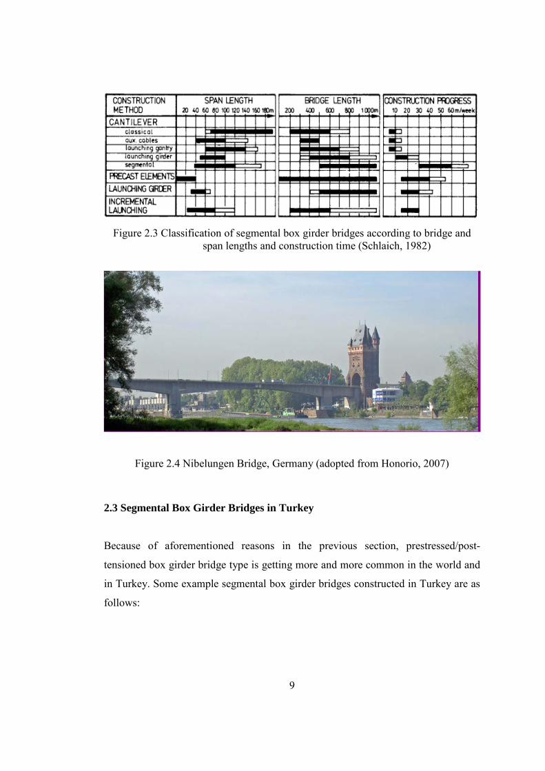
Figure 2.3 Classification of segmental box girder bridges according to bridge and
span lengths and construction time (Schlaich, 1982) ................................................... 9
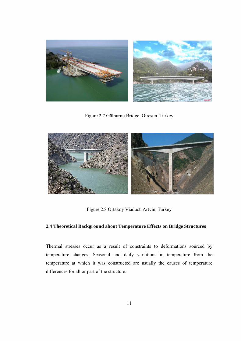
Figure 2.4 Nibelungen Bridge, Germany (adopted from Honorio, 2007) ................... 9
Figure 2.5 Kömürhan Bridge, Malatya-Elazığ Turkey .............................................. 10
Figure 2.6 Imrahor Viaduct, Ankara Turkey ............................................................. 10
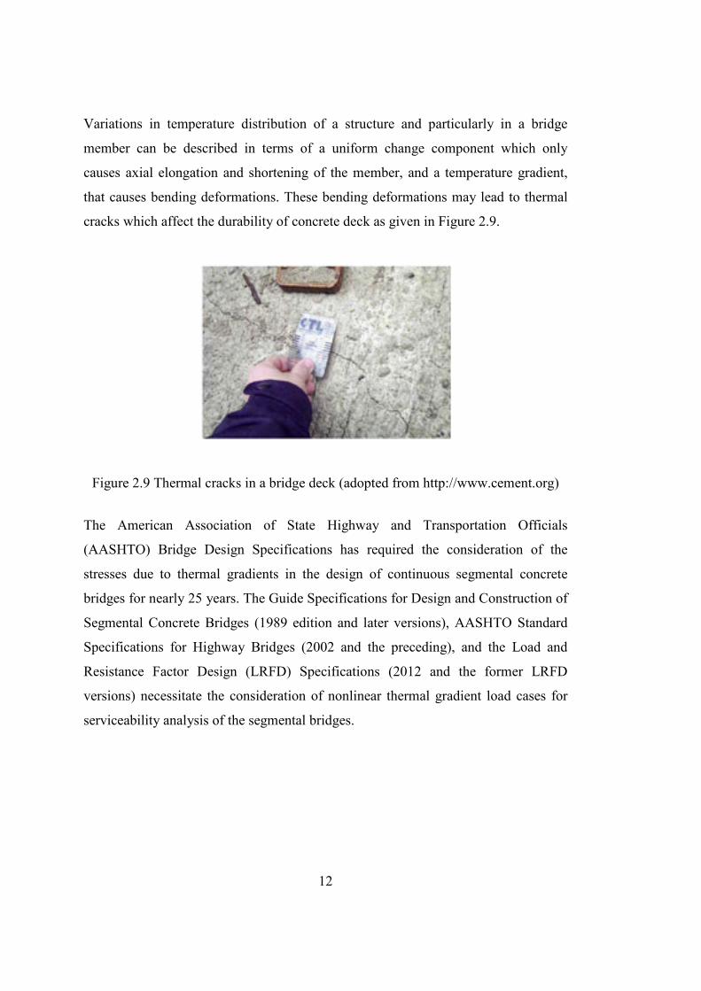
Figure 2.7 Gülburnu Bridge, Giresun, Turkey ........................................................... 11
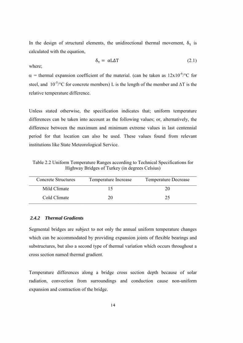
Figure 2.8 Ortaköy Viaduct, Artvin, Turkey .............................................................. 11
Figure 2.9 Thermal cracks in a bridge deck (adopted from http://www.cement.org) 12
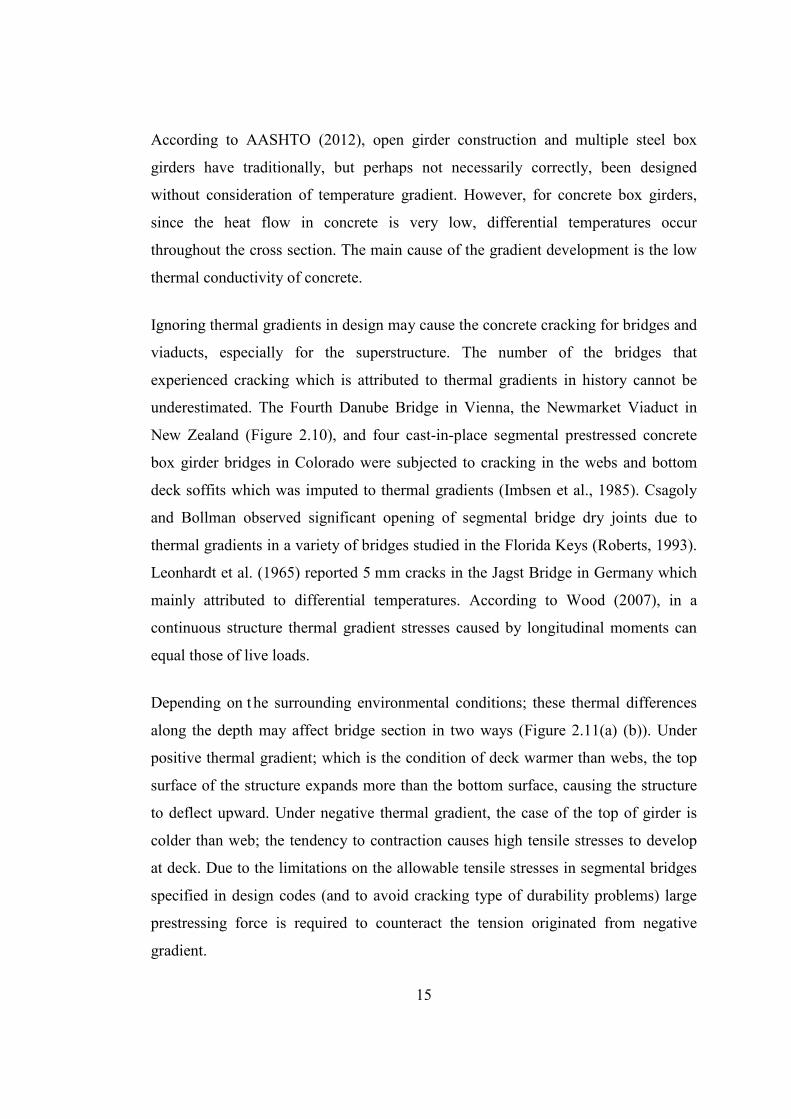
Figure 2.10 Replacement of Newmarket Viaduct with a more sustainable new
structure ...................................................................................................................... 16
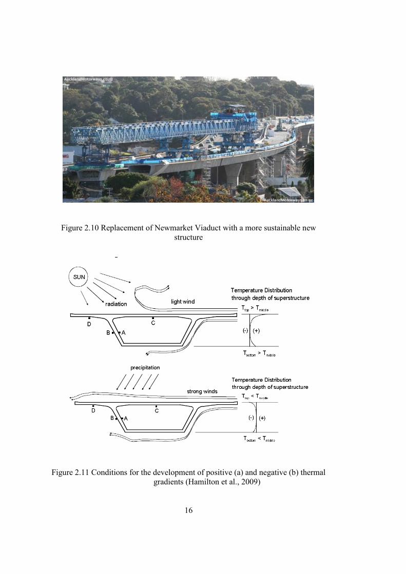
Figure 2.11 Conditions for the development of positive (a) and negative (b) thermal
gradients (Hamilton et al., 2009)................................................................................ 16
Figure 2.12 Factors affecting thermal gradient (Zhou et al., 2013) ........................... 18
Figure 2.13 Determinate beam subjected to linear gradient. (Roberts et al., 1993) ... 19
Figure 2.14 Directions showing the depth (y) and the width (z) of the structure ...... 20
Figure 2.15 Beams subjected to non-linear gradient (Roberts, 1993)........................ 22
Figure 2.16. Indeterminate beam subjected to non-linear gradient (Roberts, 1993).. 24
Figure 2.17 Stress components for indeterminate structures caused by vertical
thermal gradient ......................................................................................................... 26
Figure 2.18 Positive vertical temperature gradient in concrete and steel
superstructures (after AASHTO 1999). ..................................................................... 29
Figure 2.19 Solar radiation zones for the United States, AASHTO (the same from
1989 to 2012) ............................................................................................................. 30

xviii
Figure 2.20 Evolvement of positive and negative thermal gradients for Zone 3 (for
superstructure depths greater than 2ft, AASHTO 1989, 1994, 1999) ........................ 31
Figure 2.21 Temperature difference values for various concrete bridge deck types. 45
Figure 3.1. 16 representative cities selected for the thermal gradient analysis .......... 48
Figure 3.2Annual Monthly Averaged Direct Normal Radiation of Turkey
(kWh/m2/day) ............................................................................................................ 50
Figure 3.3 Annual Monthly Averaged Direct Normal Radiation of the U.S.A
(kWh/m2/day) ............................................................................................................ 51
Figure 3.4 Map of Turkey with latitude and longitudes and proposed solar radiation
zones ........................................................................................................................... 51
Figure 3.5 Map of the USA with latitude and longitudes and AASHTO solar
radiation zone map (AASHTO 1989a~AASHTO LRFD2010 Figure 3.12.3-1) ....... 51
Figure 3.6 Solar Radiation data for Ankara between Jan.2012-Dec.2012 ................. 52
Figure 3.7 Temperature data for Ankara between 01.01.2012-31.12.2012 ............... 52
Figure 3.8 Solar Radiation data for Istanbul between Jan.2012-Dec.2012 ................ 53
Figure 3.9 Temperature data for Istanbul between 01.01.2012-31.12.2012 .............. 53
Figure 4.1 Bridge girder cross section used in the analysis with its dimensions in mm
.................................................................................................................................... 60
Figure 4.2 Elevation view of the bridge (Adopted from Theryo, 2005) .................... 60
Figure 4.3 Finite element model of the girder and the line along which the readings
are taken ..................................................................................................................... 64
Figure 4.4 An example Panthalassa output visualization for 23.03.12, 2p.m.(GMT+2)
.................................................................................................................................... 64
Figure 4.5 Maximum measured positive gradients (a) and negative gradients (b) in
Ankara compared to recommended AASHTO Zone 1 and Turkey Zone 1. .............. 66
Figure 4.6 Maximum measured positive gradients (a) and negative gradients (b) in
İstanbul compared to recommended AASHTO Zone 2 and Turkey Zone 2. ............ 67
Figure 4.7 Maximum measured positive gradients for 16 city analyzed for Zone 1 (a)
and Zone 2 (b) compared to recommended AASHTO and Turkey Zone 1 and 2. .... 68
xix
Figure 4.8 T1 value for Ankara from Zone 1 for the day with highest positive
gradient 05.06.2012 (a) and for the day which the most severe negative gradient
occurs, 15.08.2012 (b) ................................................................................................ 69
Figure 4.9 T1 value for İstanbul from Zone 2 for the day with highest positive
gradient 14.07.2012 (a) and for the day which the lowest negative gradient occurs,
04.12.2012 (b) ............................................................................................................ 70
Figure 4.10 Recommended thermal gradient shapes and values for positive and
negative gradient ........................................................................................................ 73
Figure 4.11 3D model of the analyzed bridge, constructed in LARSA 4D ............... 74
Figure 4.12 Segment labels of the analyzed bridge model, (a) plan view, (b) elevation
view ............................................................................................................................ 75
Figure 4.13 Comparison of LRFD Design Example restraining moment values with
the analysis values for AASHTO Zone 3 positive gradient condition ....................... 76
Figure 4.14 Comparison of LRFD Design Example top stress and bottom stress
values with the analysis values for AASHTO Zone 3 ............................................... 77
Figure 4.15 Non-linear positive temperature gradient restraining moments for Zone 1
.................................................................................................................................... 78
Figure 4.16 Non-linear negative temperature gradient restraining moments for Zone
1 .................................................................................................................................. 78
Figure 4.17 Non-linear positive temperature gradient restraining moments for Zone 2
.................................................................................................................................... 79
Figure 4.18 Non-linear negative temperature gradient restraining moments for Zone
2 .................................................................................................................................. 79
Figure 4.19 Maximum stresses at support under positive gradient for Zone 1 ......... 80
Figure 4.20 Maximum stresses at support under negative gradient for Zone 1 ........ 80
Figure 4.21 Maximum stresses at support under positive gradient for Zone 2 ......... 80
Figure 4.22 Maximum stresses at support under negative gradient for Zone 2 ........ 81
Figure 4.23 Positive thermal gradient total stresses for proposed Zone 1 ................. 81
Figure 4.24 Negative thermal gradient total stresses for proposed Zone 1 ................ 82
Figure 4.25 Positive thermal gradient total stresses for proposed Zone 2 ................. 82
Figure 4.26 Negative thermal gradient total stresses for proposed Zone 2 ................ 83
xx
Figure 4.27 Top stress values for different concrete grades caused by positive
gradient of Zone 1 ...................................................................................................... 84
Figure 4.28 Bottom stress values for different concrete grades caused by positive
gradient of Zone 1 ...................................................................................................... 84
Figure 4.29 Positive and negative moment values for various truck loads ................ 87
Figure 4.30 Maximum and minimum truck stresses for mid-span ............................ 87
Figure 4.31 Maximum and minimum truck stresses for support ............................... 88
Figure 4.32 Zone 1 maximum compression and tension stresses for mid-span ......... 89
Figure 4.33 Zone 1 maximum compression and tension stresses for support............ 89
Figure 4.34 Zone 2 maximum compression and tension stresses for mid-span ......... 90
Figure 4.35 Zone 2 maximum compression and tension stresses for support............ 90
Figure 4.36 Compression stress proportions on the thermal gradient case included
load combinations for Zone 1 ..................................................................................... 91
Figure 4.37 Tension stress proportions on the thermal gradient case included load
combinations for Zone 1 ............................................................................................ 92
Figure 4.38 Compression stress proportions on the thermal gradient case included
load combinations for Zone 2 ..................................................................................... 93
Figure 4.39 Tension stress proportions on the thermal gradient case included load
combinations for Zone 2 ............................................................................................ 94
Figure A.1 Equivalent force and stress diagram for positive and negative gradient 106
Figure A.2 Equivalent I-section for the example box girder section ....................... 106
Figure A.3 Equivalent section dimensions and the applied gradient ....................... 107
Figure B.1 Solar radiation data for Adana between Jan.2012-Dec.2012 ................. 113
Figure B.2 Temperature data for Adana between Jan.2012-Dec.2012 .................... 113
Figure B.3 Solar radiation data for Ankara between Jan.2012-Dec.2012 ................ 114
Figure B.4 Temperature data for Ankara between Jan.2012-Dec.2012 ................... 114
Figure B.5 Solar radiation data for Antalya between Jan.2012-Dec.2012 ............... 115
Figure B.6 Temperature data for Antalya between Jan.2012-Dec.2012 .................. 115
Figure B.7 Solar radiation data for Bingöl between Jan.2012-Dec.2012 ................ 116
Figure B.8 Temperature data for Bingöl between Jan.2012-Dec.2012 .................... 116
Figure B.9 Solar radiation data for Bursa between Jan.2012-Dec.2012 .................. 117
xxi
Figure B.10 Temperature data for Bursa between Jan.2012-Dec.2012 ................... 117
Figure B.11 Solar radiation data for Çanakkale between Jan.2012-Dec.2012 ........ 118
Figure B.12 Temperature data for Çanakkale between Jan.2012-Dec.2012............ 118
Figure B.13 Solar radiation data for Edirne between Jan.2012-Dec.2012............... 119
Figure B.14 Temperature data for Edirne between Jan.2012-Dec.2012 .................. 119
Figure B.15 Solar radiation data for Erzurum between Jan.2012-Dec.2012 ........... 120
Figure B.16 Temperature data for Erzurum between Jan.2012-Dec.2012 .............. 120
Figure B.17 Solar radiation data for Gaziantep between Jan.2012-Dec.2012 ......... 121
Figure B.18 Temperature data for Gaziantep between Jan.2012-Dec.2012 ............ 121
Figure B.19 Solar radiation data for İstanbul between Jan.2012-Dec.2012 ............ 122
Figure B.20 Temperature data for İstanbul between Jan.2012-Dec.2012 ............... 122
Figure B.21 Solar radiation data for İzmir between Jan.2012-Dec.2012................. 123
Figure B.22 Temperature data for İzmir between Jan.2012-Dec.2012 .................... 123
Figure B.23 Solar radiation data for Kars between Jan.2012-Dec.2012 .................. 124
Figure B.24 Temperature data for Kars between Jan.2012-Dec.2012 ..................... 124
Figure B.25 Solar radiation data for Muğla between Jan.2012-Dec.2012 ............... 125
Figure B.26 Temperature data for Muğla between Jan.2012-Dec.2012 .................. 125
Figure B.27 Solar radiation data for Samsun between Jan.2012-Dec.2012 ............. 126
Figure B.28 Temperature data for Samsun between Jan.2012-Dec.2012 ................ 126
Figure B.29 Solar radiation data for Trabzon between Jan.2012-Dec.2012 ............ 127
Figure B.30 Temperature data for Trabzon between Jan.2012-Dec.2012 ............... 127
Figure B.31 Solar radiation data for Van between Jan.2012-Dec.2012................... 128
Figure B.32 Temperature data for Van between Jan.2012-Dec.2012 ..................... 128

xxii
LIST OF ABBREVIATIONS
AASHTO American Association of State Highway and Transportation Officials
AE Absolute error
ASBI American Segmental Bridge Institute
ASD Allowable stress design
ASHRAE American Society of Heating, Refrigerating and Air-Conditioning
Engineers
B Buoyancy
BL Blast loading
BR Vehicular braking force
CE Vehicular centrifugal force
CR Force effects due to creep
CT Vehicular collision force
CV Vessel collision force
DC Dead load of structural components and nonstructural attachments
DD Downdrag force
DL Structure dead load
DT Gradient Loading
DW Dead load of wearing surfaces and utilities
EE Earth Pressure
EH Horizontal earth pressure load
EL Miscellaneous locked-in force effects resulting from the construction
process, including jacking apart of cantilevers in segmental
construction
EQ Earthquake load

xxiii
ES Earth surcharge load
EV Vertical pressure from dead load of earth fill
FHWA Federal Highway Administration
FR Friction load
GDH General Directorate of Highways
GMPE Ground Motion Prediction Equation
IC Ice load
IM Vehicular dynamic load allowance
KAMAG Support Program for Research and Development Projects of Public
Institutions (in Turkish)
LFD Load Factor Design
LL Vehicular live load
LRFD Load and Resistance Factor Design
LS Live load surcharge
METU Middle East Technical University
MBE Mean bias error
MPE Mean percentage error
NASA National Aeronautics and Space Administration
NCHRP National Cooperative Highway Research Program
NOAA National Oceanic and Atmospheric Administration
PCI Prestressed Concrete Institute
PL Pedestrian live load
PTI Post Tensioning Institute
PS Secondary forces from post-tensioning
R Rib shortening
RMSE Root mean square error
RPE Relative percentage error
S Shrinkage
SDL Superimposed dead load

xxiv
SE Standard error
SE Force effect due to settlement
SF Stream flow pressure
SH Force effects due to shrinkage
SSE Surface Meteorology and Solar Energy
T Temperature loading in AASHTO Standard Specifications
T’ Temperature loading in AASHTO Guide Specifications for Design
and Construction of Segmental Concrete Bridges
T1 Temperature at the top of the section
T2 Temperature at 10 cm below the top of the section
T3 Temperature at the bottom of the section
TG Force effect due to temperature gradient
TU Force effect due to uniform temperature
TSMS Turkish State Meteorological Service
TÜBİTAK Scientific and Technological Research Council of Turkey (in Turkish)
WA Water load and stream pressure
WL Wind on live load
WS Wind load on structure
WSD Working stress design
1
CHAPTER 1
1.1 General
Segmental concrete box bridges are subject to not only the annual uniform
temperature changes -which can be accommodated by providing expansion joints,
flexible bearings or low lateral stiffness substructures-, but also a second type of
thermal variation which occurs throughout a cross section, named, thermal gradient
(or temperature gradient). Solar radiation induced temperature differences along the
depth of bridge cross section are mainly due to convection from surroundings. Also,
conduction of heat cause non-uniform expansion and contraction of a b ridge. The
thermal change through the depth may affect bridge section in two ways. Under
positive thermal gradient; which is the condition of deck is warmer than webs, the
top surface of the structure expands more than the bottom surface, causing the
structure to deflect upward, and under negative thermal gradient, the case of the top
of girder is colder than web, the tendency to contraction causes tensile stresses to
develop at deck which cause cracking type of problems.
Positive gradient gets higher when several days of cool weather is followed by
unclouded warm days with intense solar radiation and light winds. A maximum
negative gradient takes place when several days of warm weather is followed by a
severe cold weather and rain cooling the deck occurs. The cause of large gradients is
a result of low conductivity of concrete that the heat gain cannot be transferred
quickly to other parts of the cross section.
1. INTRODUCTION
2
In Germany, Austria, New Zealand, State of Colorado, and State of Florida
significant cracks are reported which are attributed to the thermal gradients.
In addition to the cracking and serviceability problems; since the thermal gradient
profile is nonlinear, compatibility stresses are also generated to satisfy plane sections
remain plane assumption of Bernoulli. Furthermore; boundary conditional restrains
cause axial and bending stresses to develop in the cross section. According to Wood
(2007), in a continuous structure thermal gradient stresses caused by longitudinal
moments can equal those of live loads.
The non-linear temperature difference through the depth of section causes huge
thermal stresses that additional prestressing requirement arises besides the ones for
dead and live load of box girder in order not to exceed mainly the allowable tensile
stress limitations.
1.2 Aim and Scope The main objective of this study is to construct a comprehensive solar radiation map
for Turkey using hourly solar radiation and temperature data to recommend vertical
design gradient values, especially for box girder bridges, which are subjected to high
compressive and tensile stress values that may result in exceedance of allowable
limits for concrete.
Since the nonlinear thermal gradients are considered only in serviceability checks; do
not affect the ultimate strength condition controls of a bridge, and after the condition
of crack development, the stress causing forces are relieved; it is argued by some
researchers that, designing for thermal stresses as high as those determined
analytically can produce overly-conservative and costly structures. In this study, it is
intended to investigate the role of thermal gradient loads on t he overall load
resultants of a bridge.

3
After the current Introduction Chapter, In Chapter 2, br ief information about box
girder bridges, segmental bridge design in the world and Turkey is given. After that,
the theoretical background about temperature effects including uniform temperature
and thermal gradient caused differences is given. The major causes of thermal
gradients and their effects on the structure, especially bridge superstructure are
examined. State of art of temperature gradient subject; historical development and
previous studies of other researchers across the world on this issue are summarized,
and suggested formulas in the literature to predict temperature gradients are
reviewed. Then, the provisions regarding to the thermal gradients in design codes of
the U.S., Europe and Turkey are summarized.
In Chapter 3, solar zone mapping of Turkey is done. AASHTO bridge specifications
recommends the use of thermal gradient loads in design since 1989 and in this
specification; the U.S. is divided into four zones per the country’s solar radiation
zones and some gradient values are given to be applied through the depth of the
girder. In this study, a similar map for Turkey is constructed to be used in design of
segmental bridges. In order to do this, temperature and solar radiation data of sixteen
cities from two recommended solar radiation zones of Turkey are collected and
processed to be applied to a box girder bridge section which is constructed in a finite
element analysis program to see the thermal differences through the depth of the
girder. Then, thermal gradient shapes and design gradient values are constituted
accordingly.
In chapter 4, suggested positive and negative thermal gradients are applied a bridge
model. The compressive and tensile stresses and bending moments developed in the
analyzed bridge superstructure are obtained to see the amount of additional
prestressing requirement. In the final step, the results are tabulated to be compared
with the loads caused by other design load cases to see the effect of vertical gradients
on the box girder bridge design. In the following figure, a flowchart of the study is
given.

4
Rev
iew
of L
itera
ture
Box
Gird
er
Brid
ges
Segm
enta
l B
ridge
sTe
mpe
ratu
re
Effe
cts
Uni
form
Te
mpe
ratu
reTh
erm
al
Gra
dien
tCau
ses o
f Te
mpe
ratu
re
Diff
eren
ces
Stru
ctur
al
Res
pons
eH
isto
rical
D
evel
opm
ent
Tem
pera
ture
G
radi
ent
Form
ulas
Cur
rent
D
esig
n Pr
actic
e
Sola
r Zon
e M
appi
ngInfo
rmat
ion
Abo
ut
AA
SHTO
AA
SHTO
Lo
ad
Com
bina
tions
Euro
code
R
equi
rem
ents
YK
İTŞ
Req
uire
men
ts
Pro
ject
In
form
atio
nD
ata
Col
lect
ion
Stat
istic
al
Com
paris
on
Ther
mal
Gra
dien
t Ana
ysis
Brid
ge M
odel
Ther
mal
Gra
dien
t Sh
ape
and
Val
ues
Res
ulta
nt S
tress
an
d M
omen
tsC
ompa
rison
of R
esul
ts
with
Oth
er L
oad
Type
s’
Figu
re 1
.1 F
low
char
t for
the
outli
ne o
f the
stud
y

5
CHAPTER 2
2. LITERATURE REVIEW
2.1 Information about Box Girder Bridges “When the history of our time is written, posterity will know us not by a cathedral or
temple, but by a bridge”
- Montgomery Shuyler (1877), writing about John Roebling’s Brooklyn Bridge
Dated from the ancient times, mankind has a general desire to make an astonishing
impact among the observers about the illustriousness and enormousness when
speaking about large scale constructions. Due to their size and importance, these
types of structures unequivocally create an impact and, in addition to their function
to serve securely and safely connection, the structures turn into a representative
monument of the place they were built.
The basic function of a bridge is to assist human by being to pass over geographical
obstacles, and as these obstacles kept getting bigger, distances get longer, man had
not only do find new ways of reaching the other side but also improved the
aesthetics and design of bridges.
For larger span lengths, dead load of the structure gains importance and in order to
reduce the dead load, removal of the not fully utilized parts of the section (material
near center of gravity contributes very little for flexure and hence can be removed)
led to cellular or box girder structures.
6
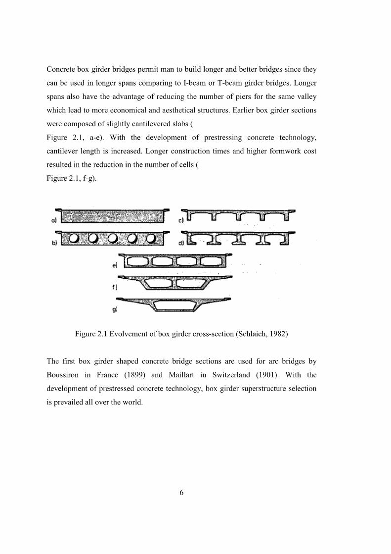
Concrete box girder bridges permit man to build longer and better bridges since they
can be used in longer spans comparing to I-beam or T-beam girder bridges. Longer
spans also have the advantage of reducing the number of piers for the same valley
which lead to more economical and aesthetical structures. Earlier box girder sections
were composed of slightly cantilevered slabs (
Figure 2.1, a-e). With the development of prestressing concrete technology,
cantilever length is increased. Longer construction times and higher formwork cost
resulted in the reduction in the number of cells (
Figure 2.1, f-g).
Figure 2.1 Evolvement of box girder cross-section (Schlaich, 1982) The first box girder shaped concrete bridge sections are used for arc bridges by
Boussiron in France (1899) and Maillart in Switzerland (1901). With the
development of prestressed concrete technology, box girder superstructure selection
is prevailed all over the world.

7
2.2 Information about Segmental Bridge Construction Segmental bridges are concrete box girder bridges whose adjacent deck sections are
constructed using repetitive elements that are progressively connected to form a
completed structure. Segmental construction was first used in China in the seventh
century for arch bridges. The technique was used in Europe much later, in the twelfth
century (Roberts, 1993).
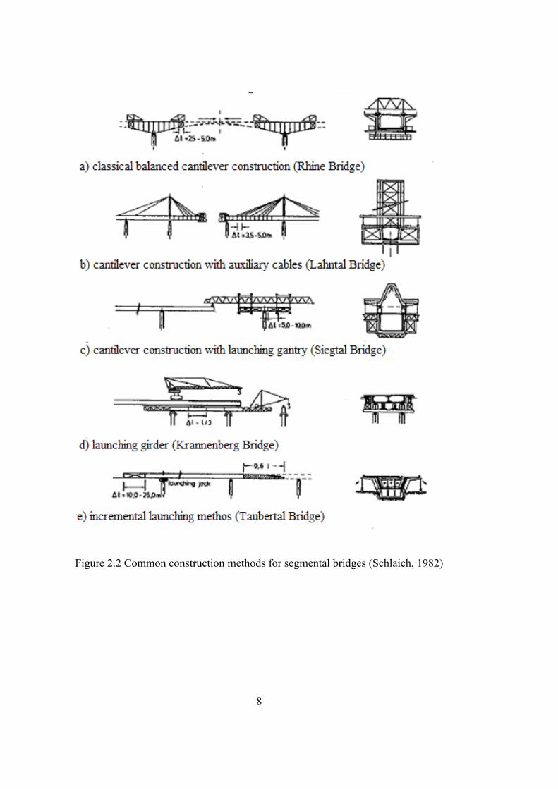
For segmental bridges the typical construction material is concrete. The common
methods that are used in segmental bridge construction and one example bridge that
has been built by that method are given schematically in Figure 2.2.
The span length, bridge length and construction process according to the selected
construction method for box girder bridge construction is tabulated by Schlaich et al.
(1982) is given in Figure 2.3. As seen in that chart, segmental, balanced cantilever
bridge construction is a fast way to build longer spans and the method is preferred
for a wide range of bridge length from 200 m to 1000 m.
In general, box girder bridges are constructed over stationary scaffolding. The most
common construction methods are the segmental balanced cantilever construction
and incremental launching method or cantilever method with launching gantry.
It was in the beginning of the 1950s that the cantilever method was realized to be
extremely useful for prestressed concrete bridge construction by a German engineer,
Ulrich Finsterwalder (1897 – 1988). His first construction was the Lahn Bridge,
1951; with a span of 62 m, but his knowledge in this particular subject resulted in the
construction of Nibelungen Bridge (Figure 2.4). This structure, with considerably
longer span lengths of 101.65 m, 114.2 m and 104.2 m captured worldwide attention
and became a mark for long span bridges, in prestressed concrete.
8
Figure 2.2 Common construction methods for segmental bridges (Schlaich, 1982)
9
Figure 2.3 Classification of segmental box girder bridges according to bridge and
span lengths and construction time (Schlaich, 1982)
Figure 2.4 Nibelungen Bridge, Germany (adopted from Honorio, 2007)
2.3 Segmental Box Girder Bridges in Turkey Because of aforementioned reasons in the previous section, prestressed/post-
tensioned box girder bridge type is getting more and more common in the world and
in Turkey. Some example segmental box girder bridges constructed in Turkey are as
follows:

10
• Malatya, Kömürhan Bridge (the one opened to service in 1986) with 76.5 m-
135 m- 76.5 m span lengths (Figure 2.5)
• Ankara, İmrahor Viaduct with 72 m - 4 x 115 m - 72 m. spans (Figure 2.6)
• Giresun, Gülburnu Bridge with 82.5 m-165 m. -82.5 m spans (Figure 2.7)
• Artvin, Ortaköy Viaduct with 78 m - 78 m spans (Figure 2.8)
Figure 2.5 Kömürhan Bridge, Malatya-Elazığ, Turkey
Figure 2.6 Imrahor Viaduct, Ankara, Turkey
11
Figure 2.7 Gülburnu Bridge, Giresun, Turkey
Figure 2.8 Ortaköy Viaduct, Artvin, Turkey 2.4 Theoretical Background about Temperature Effects on Bridge Structures
Thermal stresses occur as a result of constraints to deformations sourced by
temperature changes. Seasonal and daily variations in temperature from the
temperature at which it was constructed are usually the causes of temperature
differences for all or part of the structure.
12
Variations in temperature distribution of a structure and particularly in a bridge
member can be described in terms of a uniform change component which only
causes axial elongation and shortening of the member, and a temperature gradient,
that causes bending deformations. These bending deformations may lead to thermal
cracks which affect the durability of concrete deck as given in Figure 2.9.
Figure 2.9 Thermal cracks in a bridge deck (adopted from http://www.cement.org)
The American Association of State Highway and Transportation Officials
(AASHTO) Bridge Design Specifications has required the consideration of the
stresses due to thermal gradients in the design of continuous segmental concrete
bridges for nearly 25 years. The Guide Specifications for Design and Construction of
Segmental Concrete Bridges (1989 edition and later versions), AASHTO Standard
Specifications for Highway Bridges (2002 and the preceding), and the Load and
Resistance Factor Design (LRFD) Specifications (2012 and the former LRFD
versions) necessitate the consideration of nonlinear thermal gradient load cases for
serviceability analysis of the segmental bridges.

13
2.4.1 Uniform Temperature Changes The uniform temperature changes along the length of the bridge cause uniform
expansion or contraction of the unrestrained superstructure, which leads to the
development of axial forces if the structure is restrained against this deformation.
AASHTO (2012) considers the deformations due to uniform temperature change in
design of concrete deck bridges having concrete or steel girders. The temperature
range should be taken according to climate type of the location and the material used
according to Table 2.1 or selected according to the Tmax design Tmin design of the
contour maps of the country.
Table 2.1 Uniform Temperature Ranges According to AASHTO 2012 (in degrees
Celsius)
Climate Steel or Aluminum Concrete Wood
Moderate -17 to 49 -12 to 27 -12 to 24
Cold -34 to 49 -17 to 27 -17 to 24
Here, the number of freezing days is the main factor determining the climate type. If
the number of freezing days is less than 14 the climate is considered to be moderate
and freezing days are the days on which average temperature is less than 32°F (0°C).
According to Technical Specifications for Highway Bridges of Turkey (Yol
Köprüleri için Teknik Şartname in Turkish, 1973) thermal stresses and deformations
because of uniform temperature changes should be considered in design of highway
bridges. The decrease and increase amounts of surrounding air temperature is taken
into account according to predecided quantities during the construction of the
structure according to the region it will be build (Table 2.2).
14
In the design of structural elements, the unidirectional thermal movement, δτ is
calculated with the equation,
δτ = αL∆T (2.1) where;
α = thermal expansion coefficient of the material. (can be taken as 12x10-6/°C for
steel, and 10-5/°C for concrete members) L is the length of the member and ∆T is the
relative temperature difference.
Unless stated otherwise, the specification indicates that; uniform temperature
differences can be taken into account as the following values; or, alternatively, the
difference between the maximum and minimum extreme values in last centennial
period for that location can also be used. These values found from relevant
institutions like State Meteorological Service.
Table 2.2 Uniform Temperature Ranges according to Technical Specifications for Highway Bridges of Turkey (in degrees Celsius)
Concrete Structures Temperature Increase Temperature Decrease
Mild Climate 15 20
Cold Climate 20 25
2.4.2 Thermal Gradients Segmental bridges are subject to not only the annual uniform temperature changes
which can be accommodated by providing expansion joints of flexible bearings and
substructures, but also a second type of thermal variation which occurs throughout a
cross section named thermal gradient.
Temperature differences along a bridge cross section depth because of solar
radiation, convection from surroundings and conduction cause non-uniform
expansion and contraction of the bridge.
15
According to AASHTO (2012), open girder construction and multiple steel box
girders have traditionally, but perhaps not necessarily correctly, been designed
without consideration of temperature gradient. However, for concrete box girders,
since the heat flow in concrete is very low, differential temperatures occur
throughout the cross section. The main cause of the gradient development is the low
thermal conductivity of concrete.
Ignoring thermal gradients in design may cause the concrete cracking for bridges and
viaducts, especially for the superstructure. The number of the bridges that
experienced cracking which is attributed to thermal gradients in history cannot be
underestimated. The Fourth Danube Bridge in Vienna, the Newmarket Viaduct in
New Zealand (Figure 2.10), and four cast-in-place segmental prestressed concrete
box girder bridges in Colorado were subjected to cracking in the webs and bottom
deck soffits which was imputed to thermal gradients (Imbsen et al., 1985). Csagoly
and Bollman observed significant opening of segmental bridge dry joints due to
thermal gradients in a variety of bridges studied in the Florida Keys (Roberts, 1993).
Leonhardt et al. (1965) reported 5 mm cracks in the Jagst Bridge in Germany which
mainly attributed to differential temperatures. According to Wood (2007), in a
continuous structure thermal gradient stresses caused by longitudinal moments can
equal those of live loads.
Depending on t he surrounding environmental conditions; these thermal differences
along the depth may affect bridge section in two ways (Figure 2.11(a) (b)). Under
positive thermal gradient; which is the condition of deck warmer than webs, the top
surface of the structure expands more than the bottom surface, causing the structure
to deflect upward. Under negative thermal gradient, the case of the top of girder is
colder than web; the tendency to contraction causes high tensile stresses to develop
at deck. Due to the limitations on the allowable tensile stresses in segmental bridges
specified in design codes (and to avoid cracking type of durability problems) large
prestressing force is required to counteract the tension originated from negative
gradient.
16
Figure 2.10 Replacement of Newmarket Viaduct with a more sustainable new structure
Figure 2.11 Conditions for the development of positive (a) and negative (b) thermal gradients (Hamilton et al., 2009)
17
A linear temperature gradient causes uniform curvature in an unrestrained
superstructure. If the structure is restrained against curvature (for instance restraints
from vertical supports, bridge piers); then secondary moments develop as the result
of the linear gradient. Since the thermal gradient profile is accepted as nonlinear,
compatibility stresses are generated to satisfy the assumption of Bernoulli beam
theory that plane sections remain plane. Furthermore, boundary condition restrains
cause axial and bending stresses to develop in the cross section.
Positive gradient gets higher when several days of cool weather is followed by
unclouded warm days with intense solar radiation and light winds and conversely;
negative gradient takes place when several days of warm weather is followed by
severe cold weather and rain which cools the deck. The cause of large gradients is a
result of low conductivity of concrete that the heat gain cannot be transferred quickly
to other parts of the cross section.
Temperature gradients are calculated by finding the average web temperature (the
temperature that does not remarkably change through the depth) and using it as
baseline temperature and by subtracting it from the top and bottom temperatures.
The geometry of box-girder sections may also lead to the development of transverse
thermal gradients because of a similar reason with vertical gradients; temperature
differentials occur between parts of the section that are inside and outside the box. In
AASHTO (1999); analysis for the effects of transverse thermal gradients is generally
considered unnecessary except for relatively shallow bridges with thick webs and the
usage of a plus or minus 5.5 °C transverse temperature differential in such cases is
recommended in the specification.
The detailed literature review and code provisions about temperature gradients will
be given in the coming sections.

18
2.5 Major Factors Effecting Vertical Temperature Differences in the Depth of Girder:
The principal causes of vertical temperature differences in a girder can be
summarized into 3 titles: Climatological factors, geometrical and material properties.
Primary climatological factors; solar radiation, air temperature, and wind speed
depends on geographical parameters such as latitude, longitude, altitude and also
time. Geometric factors are the differences in cross-sectional geometry, overlay
thickness, and orientation of bridge. Finally the material properties are the thermal
conductivity, color, density, specific heat, and absorptivity of bridge deck
components. The most effective of the aforementioned factors for bridge decks are
the solar radiation and air temperature (Figure 2.12). Solar radiation is the
combination of the direct radiation which is the radiation traveling on a straight line
from the sun to the earth surface, and the diffuse radiation is the sunlight that has
been scattered by molecules and particles in the atmosphere and returns down to the
surface.
Figure 2.12 Factors affecting thermal gradient (Zhou et al., 2013)

19
Thermal gradients affect the structure in many hazardous ways. In the construction
stage, the bowing of match cast segments caused by the temperature gradient during
hydration of concrete leads to the development of gaps between two adjacent
elements and that may significantly reduce the durability and the load bearing
capacity of the structure.
2.6 Structural Response of Bridges to Temperature Variations
In structures that are externally statically determinate, for which all of the external
reaction component forces can be calculated using only static equilibrium like
simple-span bridges, there will be no temperature induced stresses. For instance, if
the structure is subjected to positive linear temperature gradient, it will elongate and
camber with an upward curve and these deformations occur without leading to the
external forces or resultant stresses (Figure 2.13), and these deformations can be
accommodated by providing bearings with adequate displacement and rotation
capacities. In some skew bridges, longitudinal expansion also causes lateral
displacement.
Figure 2.13 Determinate beam subjected to linear gradient. (Roberts et al., 1993)

20
If the statically determinant structure is subjected to a non-linear temperature
gradient; the main Euler-Bernoulli beam theory of “plane sections remain plane”
assumption is valid and the gradient causes self-equilibrating stress (Eigen stress)
development. Since there will be no shear deformation, stresses will develop because
of different strains over the section should be overcome to keep the planed form. To
determine the magnitude of self-equilibrating stresses, the following steps may be
carried.
First, the member should be assumed as a fixed member at both ends with a full
restraint of elongation and rotation like Figure 2.15 (a) and the compressive or tensile
temperature gradient stress, fRT, throughout the depth, “y” of the structure (Figure
2.14) should be found by Equation (2.2) assuming fully restrained structure:
Figure 2.14 Directions showing the depth (y) and the width (z) of the structure
𝑓𝑇𝑇(𝑦) = 𝐸 𝛼 𝑇𝑇(𝑦) (2.2)
Then the restraining force PR, and the restraining moment about the z axis MzR can
be found from the following formulas (noting that the restraining force is
compressive if the temperature gradient is positive and will be explained in detail in
following sections):
y
z

21
Axial force developed from the restraint:
𝑃𝑇 = ∫ 𝑓𝑇𝑇𝑏(𝑦) 𝑑𝑦𝑦 = ∫ 𝐸 𝛼 𝑇𝑇(𝑦)𝑏(𝑦) 𝑑𝑦𝑦 (2.3)
Moment developed from the restraint conditions:
𝑀𝑀𝑇 = ∫ 𝑃𝑇 𝑦 𝑑𝑦𝑦 = ∫ 𝐸 𝛼 𝑇𝑇(𝑦)𝑏(𝑦) 𝑦 𝑑𝑦𝑦 (2.4)
where:
y=distance from the center of gravity of the cross-section
TG(y) = temperature at depth y
b(y) = section width at depth y
E and α are the modulus of elasticity and coefficient of thermal expansion of the
structure material, respectively.
If the axial and rotational restrains P and M in Figure 2.15 (a) are removed for the
case of determinate beams as in Figure 2.15(b), the remaining stress (complete
internal stress state in statically determinate structures), fSE is the self-equilibrating
stresses, the strain distribution ε(y) and curvature (φ) of the structure can be
calculated by equations:
The self-equilibrating thermal stresses:
𝑓𝑆𝑆(𝑦) = f𝑇𝑇(𝑦) − 𝑃𝑅A− 𝑀𝑀𝑅 y
𝐼𝑧= Eα TG(y) − 𝑃𝑅
A− 𝑀𝑀𝑅 y
𝐼𝑧 (2.5)
The strain distribution ε(y):
𝜀(𝑦) = 1𝑆�𝑃𝑅A− 𝑀𝑀𝑅 y
𝐼𝑧� (2.6)

22
The curvature (φ):
𝜑(𝑦) = −𝑀𝑀𝑅 y𝑆𝐼𝑧
(2.7) where:
A = cross-section area
Iz = moment of inertia of the section about the concerned axis
Noting that the net force on section originated from self-equilibrating stresses is zero.
Figure 2.15 Beams subjected to non-linear gradient (Roberts, 1993)
23
The strain corresponding to self-equilibrating thermal stresses; 𝜀𝑠𝑠(𝑦) can be
calculated from equation:
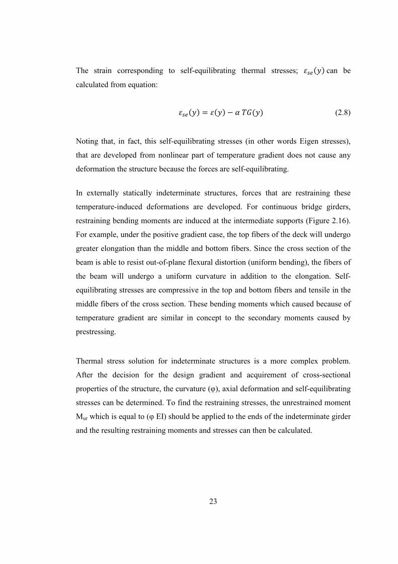
𝜀𝑠𝑠(𝑦) = 𝜀(𝑦) − 𝛼 𝑇𝑇(𝑦) (2.8)
Noting that, in fact, this self-equilibrating stresses (in other words Eigen stresses),
that are developed from nonlinear part of temperature gradient does not cause any
deformation the structure because the forces are self-equilibrating.
In externally statically indeterminate structures, forces that are restraining these
temperature-induced deformations are developed. For continuous bridge girders,
restraining bending moments are induced at the intermediate supports (Figure 2.16).
For example, under the positive gradient case, the top fibers of the deck will undergo
greater elongation than the middle and bottom fibers. Since the cross section of the
beam is able to resist out-of-plane flexural distortion (uniform bending), the fibers of
the beam will undergo a uniform curvature in addition to the elongation. Self-
equilibrating stresses are compressive in the top and bottom fibers and tensile in the
middle fibers of the cross section. These bending moments which caused because of
temperature gradient are similar in concept to the secondary moments caused by
prestressing.
Thermal stress solution for indeterminate structures is a more complex problem.
After the decision for the design gradient and acquirement of cross-sectional
properties of the structure, the curvature (φ), axial deformation and self-equilibrating
stresses can be determined. To find the restraining stresses, the unrestrained moment
Mur which is equal to (φ EI) should be applied to the ends of the indeterminate girder
and the resulting restraining moments and stresses can then be calculated.

24
Figure 2.16. Indeterminate beam subjected to non-linear gradient (Roberts, 1993)
The additional continuity stresses shall be found by performing a structural analysis
using the negative of the restraining axial force P and bending moment M given in
the Equations 2.3 and 2.4 given before.
25
The loads at the ends of the continuous structure are calculated by using structural
analysis software programs. Stresses computed from this structural analysis are then
superimposed on s tresses due to the primary restraining axial force and bending
moment to give continuity stresses. In an alternate way, the indeterminate structure
can be allowed to undergo continuity deformations due to the nonlinear gradient (that
can be obtained from Equation 2.8 given before.
By removing enough number of redundant supports to make the structure statically
determinate and the necessary reactions to implement that compatibility and
accompanying continuity stresses can then be determined by using relevant methods
(e.g. the flexibility method) afterwards. The total stress state in the continuous
structure due to the nonlinear thermal gradient is the sum of the self-equilibrating
stresses (determined previously with sectional analysis) and the continuity stresses
(Figure 2.17).
If the thermal differences are assumed to take place through the width as well as the
depth of the cross section (as mentioned before, this case could be critical in the
cases for relatively shallow bridges with thick webs), self-equilibrating thermal
stresses can be determined using Equation 2.9 through Equation 2.13, which are
two-dimensional versions of Equations 2.2 through where the directions of which y
and z axis represents were shown in Figure 2.14, previously.

26
Figure 2.17 Stress components for indeterminate structures caused by vertical thermal gradient
The vertical thermal stress assuming fully restrained structure:
𝑓𝑇𝑇(𝑀,𝑦) = (𝐸 𝛼 𝑇𝑇(𝑀,𝑦)) (2.9) Restraining axial force:
𝑃𝑇 = ∬ 𝜎𝑇𝑇(𝑦, 𝑀) 𝑑𝑀 𝑑𝑦𝑀𝑦 (2.10)
f(y) Np A
Mp yI
PrimaryStress
PrimaryStress
Ns A
Ms yI
TotalStress
ThermalComponent
AxialComponent
FlexuralComponent
Superpositionof Stresses

27
Restraining moment in z direction:
𝑀𝑀𝑇 = ∬ 𝑓𝑇𝑇(𝑦, 𝑀) 𝑦 𝑑𝑀 𝑑𝑦𝑀𝑦 (2.11)
Restraining moment in y direction:
𝑀𝑦𝑇 = ∬ 𝑓𝑇𝑇(𝑦, 𝑀) 𝑀 𝑑𝑀 𝑑𝑦𝑀𝑦 (2.12)
Self-equilibrating stress distribution:
𝑓𝑆𝑆(𝑀, 𝑦) = f𝑇𝑇(𝑀,𝑦) − 𝑃𝑅A− 𝑀𝑀𝑅 y
𝐼𝑧− 𝑀𝑦𝑅 𝑀
𝐼𝑦 (2.13)
where; Iz is the moment of inertia of section about the z axis, Iy is the moment of
inertia of the section about the y axis.
In addition to the aforementioned cases, another type of indeterminacy, internal
indeterminacy, which is the ability to calculate all of the external reaction component
forces and internal forces using only static equilibrium, also may occur over the cross
section. Because of nonlinear temperature distribution over the height of the girder,
thermally induced stresses will develop during curing and in service. However,
stresses due to external indeterminacy are unlikely to occur in curing phase because
the members are simply supported while curing.
A hand calculation is give in Appendix A. exemplifying the calculating procedure
for primary force and stresses for all of the interested solar radiation zones.
28
2.7 Previous Studies and Historical Development of Design Thermal Gradients in Design Codes
In 1967; German Code DIN 1072 (1967) was the first code to mention a differential
linear temperature distribution in the design of bridges by recommending a
temperature decreasing 5°C from upper surface to the soffit. New Zealand Code’s
recommendation (1970) considering a constant temperature in the top slab is
replaced by a highly nonlinear-sixth order curve in 1973; and once again changed
into the requirement to use a fifth order parabola for first 1200mm depth of girder
with a 57.6°F (32°C) temperature gradient in (Priestley, 1987). The first
recommendation to consider thermal gradient in segmental bridge design in the
United States was done by PCI-PTI (Prestressed Concrete Institute-Post Tensioning
Institute) in 1977 a s a constant gradient in top slab with 18°F (10°C) temperature
differential (PTI, 1977). After that Hoffman et al. (1980) made an experimental
study in Pennsylvania and proposed to use 36°F (20°C) differential, instead of PCI-
PTI’s 18°F (10°C) and; after them Elbadry et al. (1983) developed a finite element
computer program and in 1984 Cooke et al. did a similar study with prestressed
concrete bridges and reasonable agreement was found as cited by Shushkewich
(1998). In 1983 P otgieter et al. conducted a detailed study on nonlinear thermal
gradients in 26 l ocations of the United States and developed a finite difference
computer model which does heat flow analysis and predicted gradients for that
locations and they verified their results by comparing the data got from Kishwaukee
Bridge in Illinois. After that, Imbsen et al. (1985) improved Potgieter et al. (1983)’s
work and presented a comprehensive state-of-art report; “National Cooperative
Highway Research Program (NCHRP) Report 276” on thermal effects in concrete
bridges, which later formed the basis for AASHTO guide specifications regarding
thermal gradients.
Prior to AASHTO (1989c) former AASHTO Standard Specifications for Highway
Bridges were considering stresses, axial expansion and contraction only because of
uniform temperature changes and ignoring the probable stress distributions
29
throughout the depth of girder. In 1989 A ASHTO published their Guide
Specification, Thermal Effects in Concrete Bridge Superstructures (AASHTO
1989a), which was based on NCHRP Report 276. The AASHTO Guide Specification
for Design and Construction of Segmental Concrete Bridges (AASHTO 1989b)
required the consideration of thermal gradients in the design of all segmental bridges.
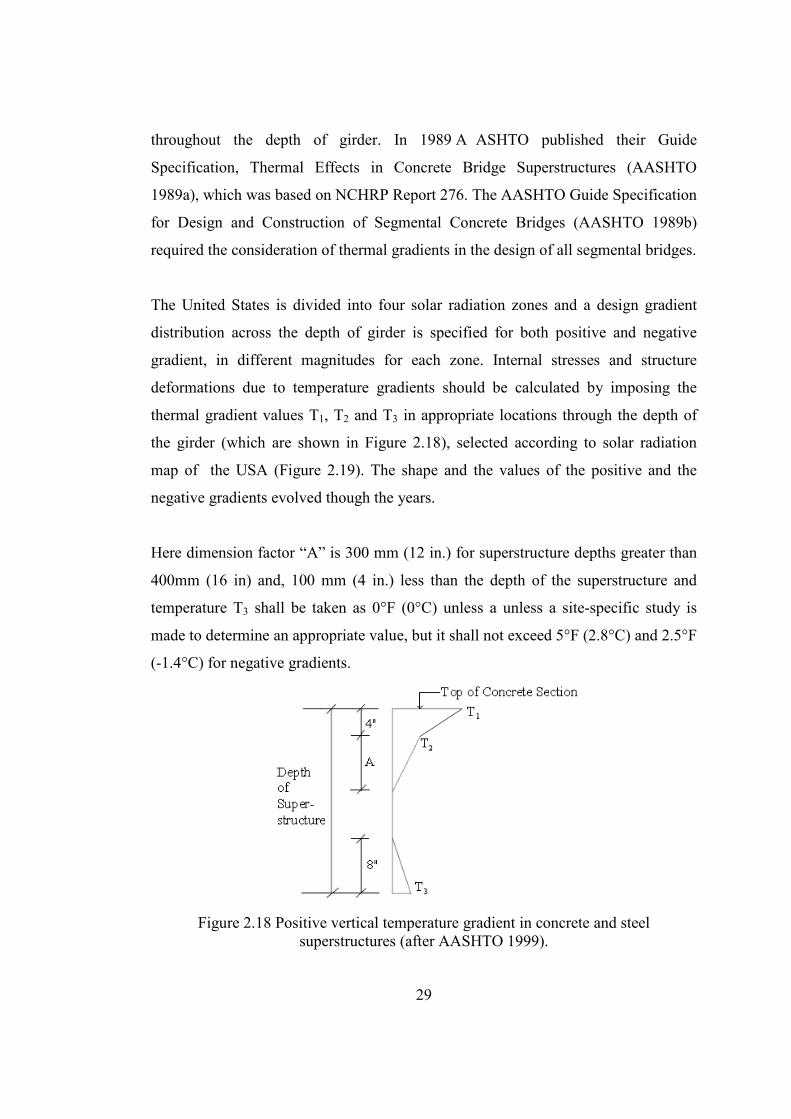
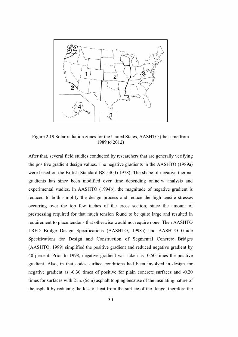
The United States is divided into four solar radiation zones and a design gradient
distribution across the depth of girder is specified for both positive and negative
gradient, in different magnitudes for each zone. Internal stresses and structure
deformations due to temperature gradients should be calculated by imposing the
thermal gradient values T1, T2 and T3 in appropriate locations through the depth of
the girder (which are shown in Figure 2.18), selected according to solar radiation
map of the USA (Figure 2.19). The shape and the values of the positive and the
negative gradients evolved though the years.
Here dimension factor “A” is 300 mm (12 in.) for superstructure depths greater than
400mm (16 in) and, 100 mm (4 in.) less than the depth of the superstructure and
temperature T3 shall be taken as 0°F (0°C) unless a unless a site-specific study is
made to determine an appropriate value, but it shall not exceed 5°F (2.8°C) and 2.5°F
(-1.4°C) for negative gradients.
Figure 2.18 Positive vertical temperature gradient in concrete and steel
superstructures (after AASHTO 1999).
30
Figure 2.19 Solar radiation zones for the United States, AASHTO (the same from 1989 to 2012)
After that, several field studies conducted by researchers that are generally verifying
the positive gradient design values. The negative gradients in the AASHTO (1989a)
were based on the British Standard BS 5400 (1978). The shape of negative thermal
gradients has since been modified over time depending on ne w analysis and
experimental studies. In AASHTO (1994b), the magnitude of negative gradient is
reduced to both simplify the design process and reduce the high tensile stresses
occurring over the top few inches of the cross section, since the amount of
prestressing required for that much tension found to be quite large and resulted in
requirement to place tendons that otherwise would not require none. Then AASHTO
LRFD Bridge Design Specifications (AASHTO, 1998a) and AASHTO Guide
Specifications for Design and Construction of Segmental Concrete Bridges
(AASHTO, 1999) simplified the positive gradient and reduced negative gradient by
40 percent. Prior to 1998, negative gradient was taken as -0.50 times the positive
gradient. Also, in that codes surface conditions had been involved in design for
negative gradient as -0.30 times of positive for plain concrete surfaces and -0.20
times for surfaces with 2 in. (5cm) asphalt topping because of the insulating nature of
the asphalt by reducing the loss of heat from the surface of the flange, therefore the
31
magnitude of thermal gradient. Moreover, prior to 1994, t hermal gradient shapes
were applicable only to superstructure depths greater than 2ft but from that on,
different superstructure depths are taken into account in design. Nonlinear thermal
gradient values which are given in Table 2.3 and the shapes of the gradients (Figure
2.18) are remained the identical after 1999 in other intermediary specifications and
also the same in latest 2012 LRFD Specifications (AASHTO, 2012).
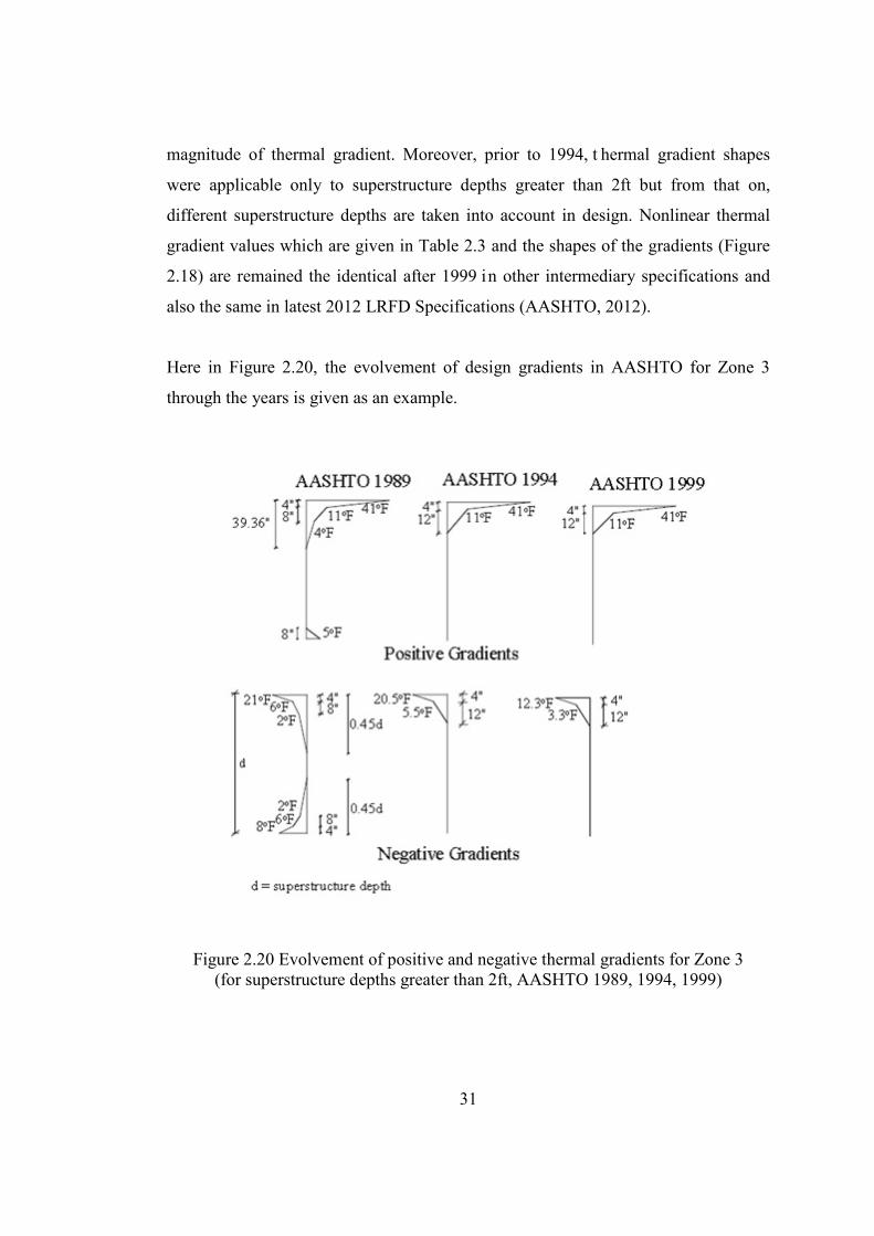
Here in Figure 2.20, the evolvement of design gradients in AASHTO for Zone 3
through the years is given as an example.
Figure 2.20 Evolvement of positive and negative thermal gradients for Zone 3 (for superstructure depths greater than 2ft, AASHTO 1989, 1994, 1999)

32
It is important to note that, in AASHTO LRFD (2012), it is stated that, the data in
Table 2.3 does not make a distinction with regard to presence or lack of asphalt
overlay for positive gradient; because, the field measurement studies of Spring
(1997) were not in conformity with each other regarding to the insulating or
contributing effect of asphalt on deck. Moreover, Roberts et al. (1993) observed the
average monitored maximum positive gradient for the no topping case is 30% less
than the value with the 2 inch (5 cm) asphalt topping for San Antonio “Y” project; in
contrast to the original analysis by Potgieter et al. (1983)’s confirmations (which
form the basis for AASHTO thermal gradients) with data from the Kishwaukee
Bridge which had an asphalt topping. Roberts et al. (1993)’s explanation to this is
that; the absorptive constant for bare concrete used in the analysis has a great impact
on the calculated gradient. Potgieter et al.’s used a high value for the absorptive
which assumed the concrete was smooth and dirty and dark colored from passing
traffic and pollution. Conversely, the concrete in the San Antonio “Y” project’ was
very light in color due to the white crushed limestone aggregate, and the surface is
roughened. Because of such possible differences in wearing coats, effect of
insulating materials above deck is ignored in AASHTO for design for positive
gradient.
Table 2.3 Positive Temperature Differentials (after AASHTO, 1999)
Zone T1 °C (°F) T2 °C (°F) 1 30 (54) 8 (14) 2 25 (46) 7 (12) 3 23 (41) 6 (11) 4 21 (38) 5 (9)
The negative gradient values are found by multiplying the values shown in Table 2.3
by -0.2 with the same shape as positive gradient for the decks with asphalt topping.
33
On the subject of thermal gradient design for segmental concrete bridges; AASHTO
LRFD (2012) is still allied to the some of the publications such as; Thermal Effects
in Concrete Bridge Superstructures (AASHTO, 1989a) and the Guide Specifications
for Design and Construction of Segmental Concrete Bridges (AASHTO, 1999),
which will be detailed in the following sections.
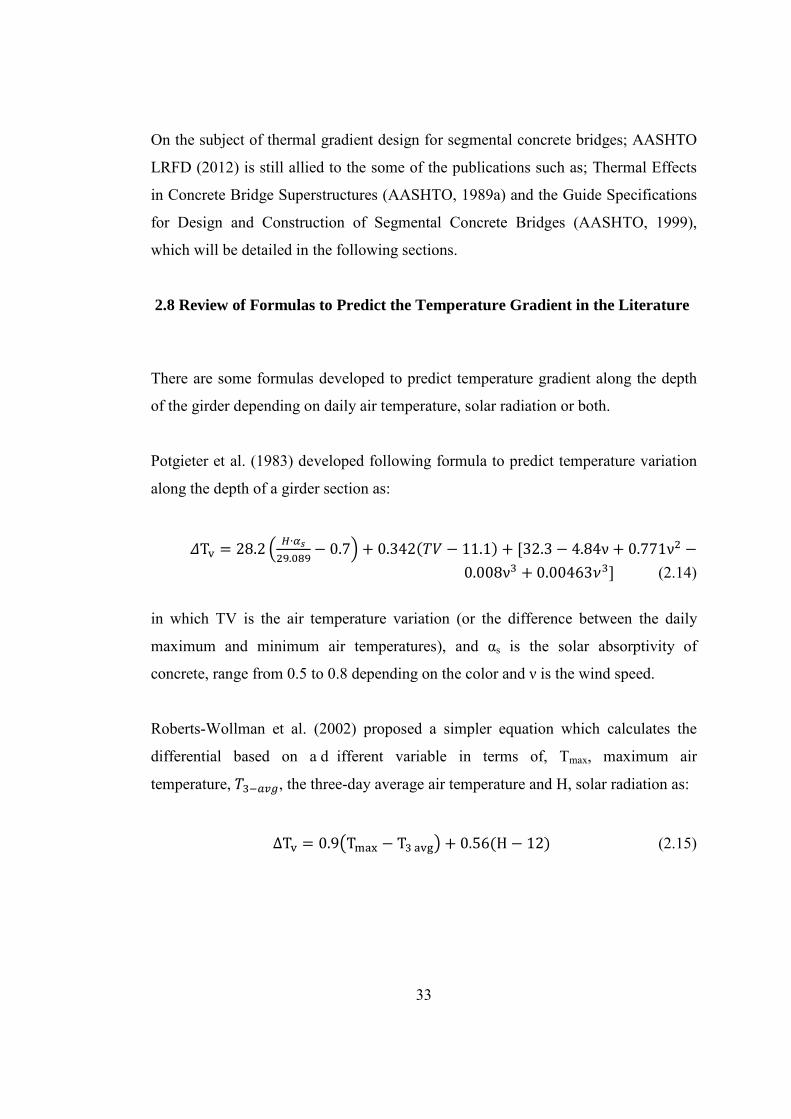
2.8 Review of Formulas to Predict the Temperature Gradient in the Literature
There are some formulas developed to predict temperature gradient along the depth
of the girder depending on daily air temperature, solar radiation or both.
Potgieter et al. (1983) developed following formula to predict temperature variation
along the depth of a girder section as:
𝛥Tv = 28.2 � 𝐻∙𝛼𝑠29.089
− 0.7� + 0.342(𝑇𝑇 − 11.1) + [32.3 − 4.84ν + 0.771ν2 −0.008ν3 + 0.00463𝜈3] (2.14)
in which TV is the air temperature variation (or the difference between the daily
maximum and minimum air temperatures), and αs is the solar absorptivity of
concrete, range from 0.5 to 0.8 depending on the color and ν is the wind speed.
Roberts-Wollman et al. (2002) proposed a simpler equation which calculates the
differential based on a d ifferent variable in terms of, Tmax, maximum air
temperature, 𝑇3−𝑎𝑎𝑎, the three-day average air temperature and H, solar radiation as:
ΔTv = 0.9�Tmax − T3 avg� + 0.56(H − 12) (2.15)
34
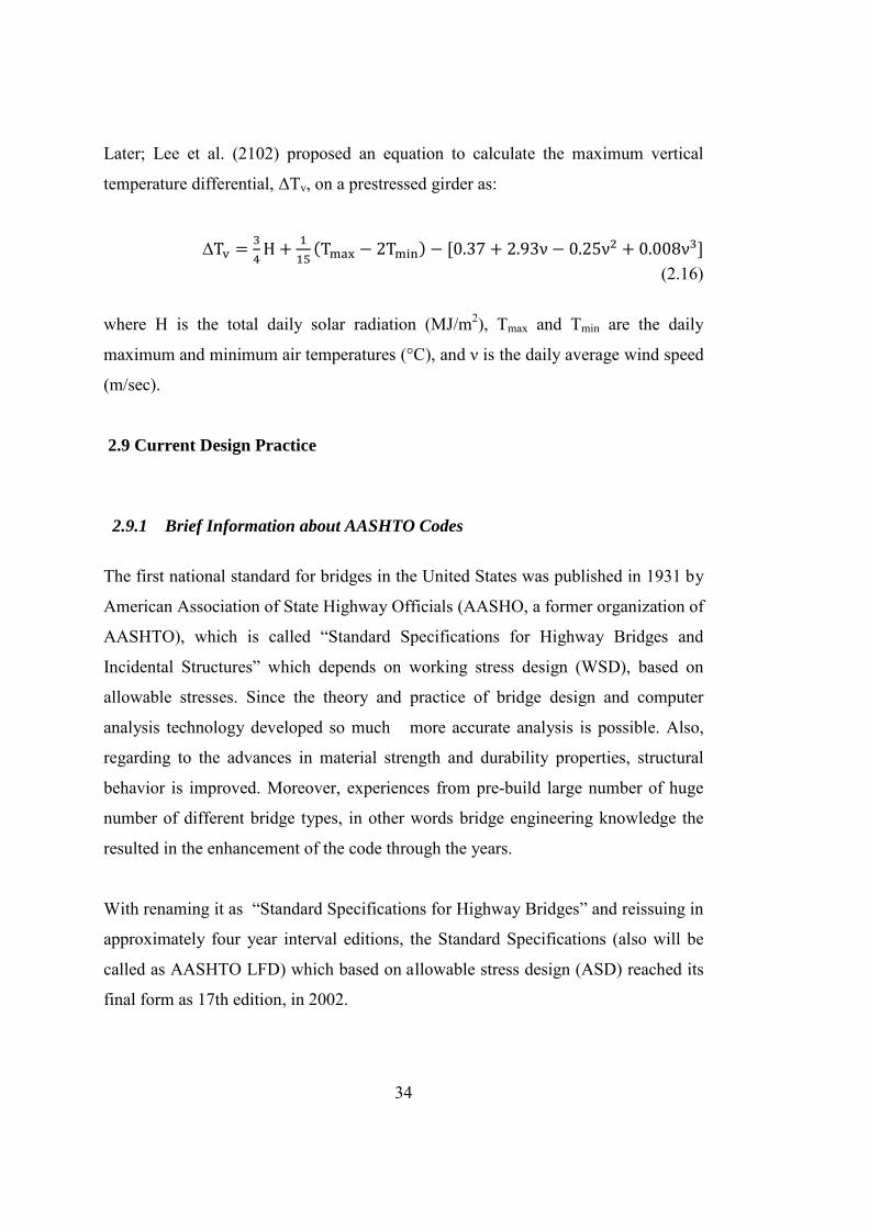
Later; Lee et al. (2102) proposed an equation to calculate the maximum vertical
temperature differential, ΔTv, on a prestressed girder as:
ΔTv = 34
H + 115
(Tmax − 2Tmin) − [0.37 + 2.93ν − 0.25ν2 + 0.008ν3] (2.16)
where H is the total daily solar radiation (MJ/m2), Tmax and Tmin are the daily
maximum and minimum air temperatures (°C), and ν is the daily average wind speed
(m/sec).
2.9 Current Design Practice
2.9.1 Brief Information about AASHTO Codes
The first national standard for bridges in the United States was published in 1931 by
American Association of State Highway Officials (AASHO, a former organization of
AASHTO), which is called “Standard Specifications for Highway Bridges and
Incidental Structures” which depends on working stress design (WSD), based on
allowable stresses. Since the theory and practice of bridge design and computer
analysis technology developed so much more accurate analysis is possible. Also,
regarding to the advances in material strength and durability properties, structural
behavior is improved. Moreover, experiences from pre-build large number of huge
number of different bridge types, in other words bridge engineering knowledge the
resulted in the enhancement of the code through the years.
With renaming it as “Standard Specifications for Highway Bridges” and reissuing in
approximately four year interval editions, the Standard Specifications (also will be
called as AASHTO LFD) which based on allowable stress design (ASD) reached its
final form as 17th edition, in 2002.

35
Extending to the recent times, the ASD specification started not to reverberate or
comprise the recently developing design philosophy, load-and-resistance factor
design (LRFD), which has been gaining importance and countenance in other areas
of structural engineering as well in the USA and in other parts of the world like
Canada and Europe.
In 1986, the Subcommittee submitted a request to the AASHTO Standing Committee
on Research to undertake an assessment of U.S. bridge design specifications, and this
task is done under the National Cooperative Highway Research Program (NCHRP),
an applied research program which is completed in 1987 aiming to review foreign
design specifications and codes, and to render recommendations based on t hese
investigations.
The main report which was a milestone of the acknowledgement of thermal gradient
in AASHTO Design Codes was the NCHRP Report 276 and the 1st edition of
AASHTO LRFD Specifications was published in 1994, the 2nd in 1998, the next in
2004, then 2007, 2010, 2012 and 2014.
After the publication of LRFD specifications; bridge design can be done according to
either of two standards to guide their designs; the long-time familiar AASHTO
Standard Specifications for Highway Bridges, and newly adopted AASHTO LRFD
Bridge Design Specifications, with its accompanying guidelines, AASHTO LRFD
Bridge Construction Specifications and AASHTO LRFD Movable Highway Bridge
Design Specifications. After 2007, the Federal Highway Administration (FHWA)
and the states have established a goal to integrate LRFD standards in all new bridge
designs.

36
Interim Specifications are usually published in the middle of the year, and revised
edition of this the specifications are generally published in at most every four years.
The Interim Specifications have the same status as AASHTO standards, and tentative
revisions are approved by at least two-thirds of the Subcommittee.
In Turkey, highway bridges are designed according to modified version of the
Standard Specifications for Highway Bridges (AASHTO LFD).
2.9.2 Corresponding Load Combinations of AASHTO Codes
Both uniform temperature and temperature gradient should be included in service
limit state load combinations. Temperature gradient may be reduced by 50% if live
load is present in service load combinations. Designers should be cautious in that for
uniform temperature load factor of 1.0 should be used when checking stresses, and
1.2 for structural deformations.
Temperature gradient may not be included in strength limit state load combinations,
while uniform temperature should. Two load factors are assigned to uniform
temperature in strength limit states like service limit states. A factor of 0.5 shall be
used for strength capacity calculations and 1.2 for structural deformations in strength
limit state calculations. Besides, it is not recommended to combine thermal gradient
with high wind forces.
In the subsequent topics, the AASHTO codes which are temperature gradient load
case will be briefly scrutinized.
37
2.9.2.1 AASHTO Standard Specifications for Highway Bridges Requirements:
AASHTO Standard Specification (2002) and prior Standard Specifications which is
widely used in bridge design does not consider thermal gradient loading for design of
bridges. Only uniform temperature changes are included in design load combinations
symbolized with T.
2.9.2.2 AASHTO Guide Specification for Highway Bridges (1989)
Requirements
This specification also only requires the consideration of thermal effects in any
bridge design by recommending to consider the stresses and movements caused by
only uniform temperature changes.
2.9.2.3 AASHTO Guide Specifications for Design and Construction of Segmental Concrete Bridges (1989) Requirements:
The temperature loading, T in the standard specification is redefined (symbolized by
T’ here) in the segmental specification as the sum of the original temperature loading
in Standard Specification, T, and thermal gradient loading (DT).
T’= T+ DT
The AASHTO Guide Specifications for Design and Construction of Segmental
Concrete Bridges (1989) ameliorates the AASHTO Guide Specifications for
Highway Bridges (1989) load cases by adding the following service load condition
which takes thermal gradient into consideration (The loads in below equations shown
in parentheses are the loads required by the AASHTO Segmental Specification and
the others are defined and required by the AASHTO Standard Specification):
(DL + SDL + EL) +EE + B +SF + R + S + (DT)

38
where
DL = structure dead load
B = buoyancy
SDL = superimposed dead load
SF = stream flow pressure
EL = Miscellaneous locked-in force effects resulting from the construction process,
including jacking apart of cantilevers in segmental construction
R = rib shortening
EE = earth pressure
S = shrinkage
Moreover, in this specification it is stated that, for load combinations that include full
live load with impact, DT can be reduced by 50 percent.
2.9.2.4 AASHTO LRFD Specification Requirements: (1994) The AASHTO LRFD divides load combinations into main categories according to
the limit s tate considered as Strength, Extreme Event, Service and Fatigue limit
states as shown in Table 2.4.
The temperature gradient effects of the 2012 edition of the AASHTO LRFD Bridge
Design Specifications are analyzed under the load combinations Strength I, Strength
II, Strength III, Strength V, Service I and Service III.
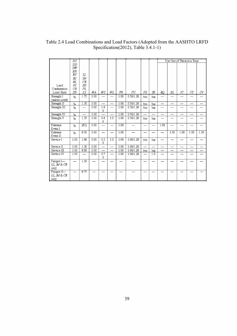
39
Table 2.4 Load Combinations and Load Factors (Adopted from the AASHTO LRFD Specification(2012), Table 3.4.1-1)

40
All permanent and transient load and force abbreviations which are stated in the table
are;
• Permanent Loads
CR = force effects due to creep
DD = downdrag force
DC = dead load of structural
components and nonstructural
attachments
DW = dead load of wearing surfaces
and utilities
EH = horizontal earth pressure load
EL = miscellaneous locked-in force
effects resulting from the construction
process, including jacking apart of
cantilevers in segmental construction
ES = earth surcharge load
EV = vertical pressure from dead load
of earth fill
PS = secondary forces from post-
tensioning
SH = force effects due to shrinkage
Transient Loads
BL = blast loading
BR = vehicular braking force
CE = vehicular centrifugal force
CT = vehicular collision force
CV = vessel collision force
EQ = earthquake load
FR = friction load
IC = ice load
IM = vehicular dynamic load
allowance
LL = vehicular live load
LS = live load surcharge
PL = pedestrian live load
SE = force effect due to settlement
TG = force effect due to temperature
gradient
TU = force effect due to uniform
temperature
WA = water load and stream pressure
WL = wind on live load
WS = wind load on structure
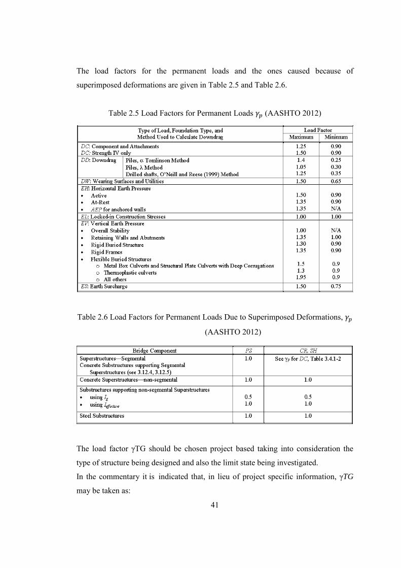
41
The load factors for the permanent loads and the ones caused because of
superimposed deformations are given in Table 2.5 and Table 2.6.
Table 2.5 Load Factors for Permanent Loads 𝛾𝑝 (AASHTO 2012)
Table 2.6 Load Factors for Permanent Loads Due to Superimposed Deformations, 𝛾𝑝
(AASHTO 2012)
The load factor γTG should be chosen project based taking into consideration the
type of structure being designed and also the limit state being investigated.
In the commentary it is indicated that, in lieu of project specific information, γTG
may be taken as:

42
• 0.0 at the strength and extreme event limit states,
• 1.0 at the service limit state when live load is not considered, and
• 0.50 at the service limit state when live load is considered.
In addition to the Table 2.4, for only segmentally constructed bridges, the following
combination also shall be investigated at the service limit state:
DC + DW + EH + EV + ES +WA+CR + SH +TG+ EL + PS
This load combination has no l ive load; hence, 100% of the temperature gradient
shall be included. In general, this load combination is the controlling equation for
segmental concrete bridge design where live load force effects are small in areas
such as the ones near the closure pours in the top of the box.
To sum up, in the scope of this study; thermal gradient included the load
combinations for segmental bridges considering the maximum load factors for
permanent loads and taking dead loads, live loads and thermal gradient load as main
variables are:
• Service I (with live load): 1.00DC+1.00DW+1.00(LL+IM)+0.50TG
• Service III (with live load): 1.00DC+1.00DW+0.80(LL+IM)+0.50TG
• Service I and III (without live load) and Service Comb. for Segmental
Bridges: 1.00DC+1.00DW+1.00TG
The stress limits for Concrete According to AASHTO LRFD (2012) Chapter 5.9.4, the stress limits for concrete
should be checked for both before the losses due to creep and shrinkage and for the
service loads after losses have occurred.

43
Temporary Stresses Before the Losses Due To Creep and Shrinkage (at the time
where prestress is applied):
• Compression Stresses:
AASHTO LRFD (2012) limits the compressive stresses including segmentally
constructed bridges, shall be 0.60 f’ci for all prestressed concrete components,
whereas AASHTO (2002) recommends the value 0.60 f’ci for pretensioned and 0.55
f’ci (MPa) for post-tensioned members, where f’ci is the compressive strength of
concrete at the time of initial prestress.
f’ci = 0.75 x fc
where f’c: compressive strength of concrete at 28 days
σall,c = 0.6 f’ci
• Tension Stresses
-For segmentally constructed bridges; longitudinal stresses through joints in the
precompressed tensile zone, for joints which does not have minimum necessary
bonded auxiliary reinforcement, tension is not allowed.
-For joints with minimum bonded auxiliary reinforcement through the joints, that
sufficiently carry the calculated tensile force at a stress of 0.5 fy (not to exceed 210
MPa); with internal tendons or external tendons, in longitudinal direction 0.63 �𝑓𝑐𝑐
tension stress is allowed.
-For transverse stresses, any type of joint may carry 0.25 �𝑓𝑐 (𝑀𝑃𝑀) tension stress.
44
Stresses at Service Limit State after Losses (for fully prestressed components):
• Compression Stresses:
Compression should be checked for Service-I Load Combination given in Table 2.4.
In segmentally constructed bridges due to the sum of effective prestress and
permanent loads, compressive stress must be less than 0.45 f’c.
σall,t = 0.45 f’c
• Tension Stresses:
For longitudinal service load combinations that involve traffic loading tension
stresses in members with bonded or unbounded prestressing tendons should be
investigated using load combination Service III specified in Table 2.4. F or
transverse analyses of box girder bridges load combination Service I should be
investigated which are involving traffic loadings.
For segmentally constructed bridges;
-Longitudinal stresses through joints in the pre-compressed tensile zone, for joints
which does not have minimum necessary bonded auxiliary reinforcement, tension is
not allowed. For joints with minimum bonded auxiliary reinforcement through the
joints, that sufficiently carry the calculated tensile force at a stress of 0.5 fy; with
internal tendons or external tendons, 0.25 �𝑓𝑐 (𝑀𝑃𝑀) tension stress is allowed.
-For transverse stresses, also the stress through joints may be 0.25 �𝑓𝑐 (𝑀𝑃𝑀) .
-For the stresses at web, in the depth of neutral axis 0.289�𝑓𝑐 (𝑀𝑃𝑀)
-For the other areas with bonded reinforcement, assuming the section is not cracked,
0.5 �fc (MPa) tension is allowed
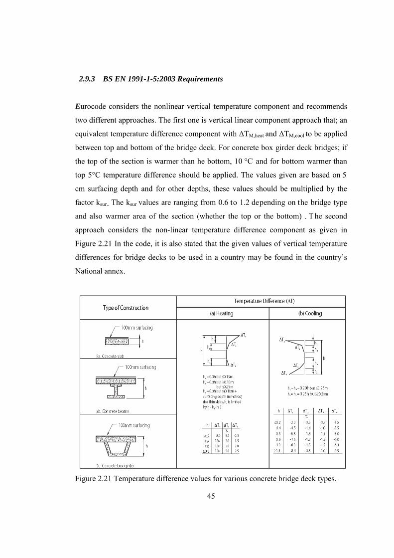
45
2.9.3 BS EN 1991-1-5:2003 Requirements
Eurocode considers the nonlinear vertical temperature component and recommends
two different approaches. The first one is vertical linear component approach that; an
equivalent temperature difference component with ΔTM,heat and ΔTM,cool to be applied
between top and bottom of the bridge deck. For concrete box girder deck bridges; if
the top of the section is warmer than he bottom, 10 °C and for bottom warmer than
top 5°C temperature difference should be applied. The values given are based on 5
cm surfacing depth and for other depths, these values should be multiplied by the
factor ksur.. The ksur values are ranging from 0.6 to 1.2 depending on the bridge type
and also warmer area of the section (whether the top or the bottom) . T he second
approach considers the non-linear temperature difference component as given in
Figure 2.21 In the code, it is also stated that the given values of vertical temperature
differences for bridge decks to be used in a country may be found in the country’s
National annex.
Figure 2.21 Temperature difference values for various concrete bridge deck types.

46
As seen in heating (top surface is warmer than web) condition, for bridge decks
deeper than 0.8m, the ΔT1 value is 13°C at most and for cooling condition; for
sections deeper than 1.5m, this value is minimum -8.4°C.
The values of Eurocode are found too small considering the analysis results of the
cities of Turkey, thus, the comparisons will be made with AASHTO instead of
Eurocode.
2.9.4 Technical Specifications for Highway Bridges of Turkey (Yol Köprüleri
için Teknik Şartname) (1982) Requirements: No requirement for thermal gradient through the depth of the structure. Only uniform
temperature effects are included (given in detail in Chapter 2.4.1)
Within the scope of a national project (TUBITAK, 110G093) a new bridge design
code for Turkey is being prepared by a large team of civil and earthquake engineers.
In this code, the use of a positive and negative thermal gradient is proposed.
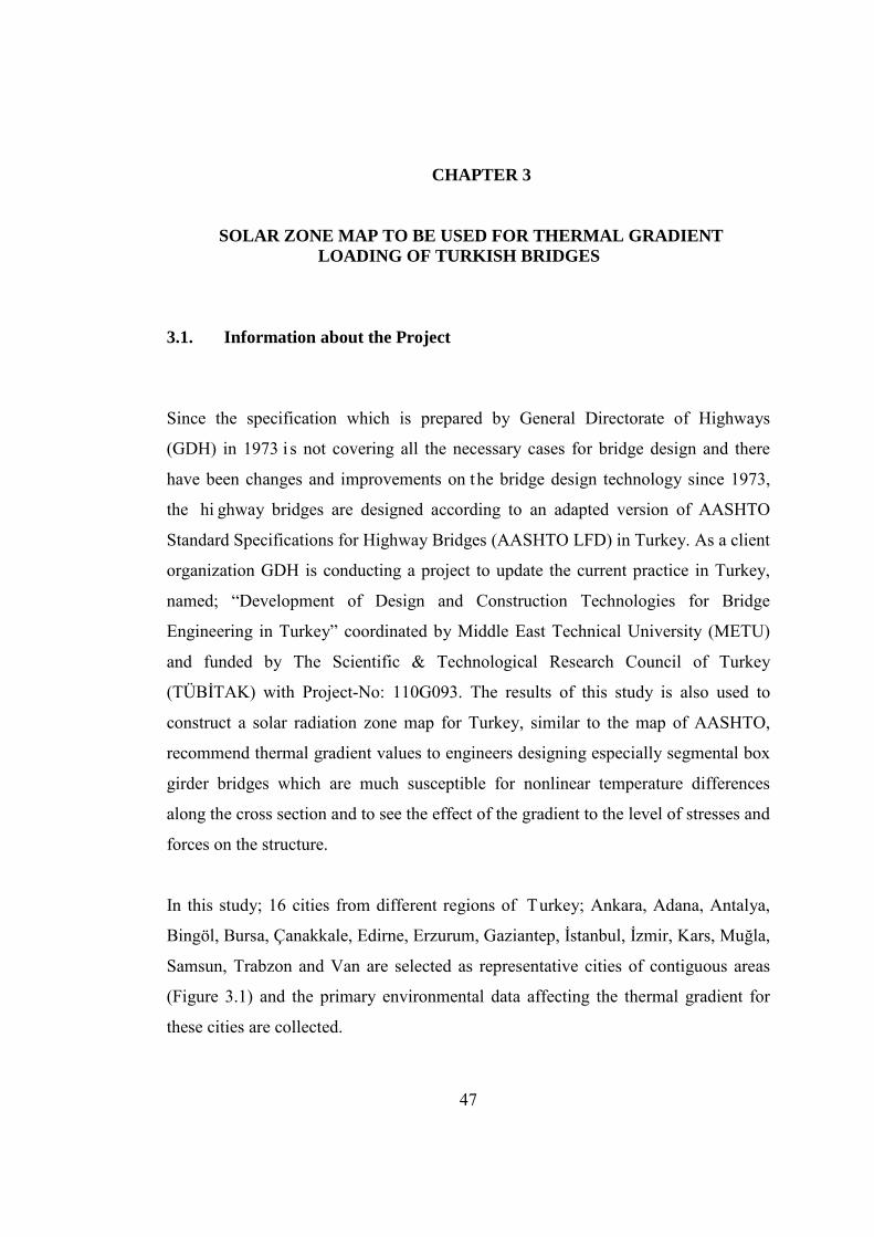
47
CHAPTER 3
3.1. Information about the Project
Since the specification which is prepared by General Directorate of Highways
(GDH) in 1973 i s not covering all the necessary cases for bridge design and there
have been changes and improvements on the bridge design technology since 1973,
the hi ghway bridges are designed according to an adapted version of AASHTO
Standard Specifications for Highway Bridges (AASHTO LFD) in Turkey. As a client
organization GDH is conducting a project to update the current practice in Turkey,
named; “Development of Design and Construction Technologies for Bridge
Engineering in Turkey” coordinated by Middle East Technical University (METU)
and funded by The Scientific & Technological Research Council of Turkey
(TÜBİTAK) with Project-No: 110G093. The results of this study is also used to
construct a solar radiation zone map for Turkey, similar to the map of AASHTO,
recommend thermal gradient values to engineers designing especially segmental box
girder bridges which are much susceptible for nonlinear temperature differences
along the cross section and to see the effect of the gradient to the level of stresses and
forces on the structure.
In this study; 16 cities from different regions of Turkey; Ankara, Adana, Antalya,
Bingöl, Bursa, Çanakkale, Edirne, Erzurum, Gaziantep, İstanbul, İzmir, Kars, Muğla,
Samsun, Trabzon and Van are selected as representative cities of contiguous areas
(Figure 3.1) and the primary environmental data affecting the thermal gradient for
these cities are collected.
3. SOLAR ZONE MAP TO BE USED FOR THERMAL GRADIENT LOADING OF TURKISH BRIDGES

48
Figure 3.1. 16 representative cities selected for the thermal gradient analysis
3.2. Collection of Data
Since the first step to construct a temperature map is to get irradiance values for
geographic regions in desired proximity, the solar radiation data for Turkey had to be
found. Solar radiation is obtained by ground measurement or satellite data.
In Turkey, Turkish State Meteorological Service (Meteoroloji Genel Müdürlüğü,
TSMS) is responsible for the measurement, collection, recording, qualifying and the
assessment of meteorological parameters. The institution is doing this by using
meteorological observations, numerical weather prediction models and remote
sensing products; and, does land, air and sea related meteorological forecasts to give
early warnings for severe meteorological events (which are temperature,
precipitation wind, pressure, snow amounts, waviness of seas, cloudiness and solar
radiation data).

49
Solar radiation observations have been made by TSMS to determine irradiance in
Turkey for a long period of time using ground measurements. These observations
mainly consist of solar insulation and sunshine duration type of data. Bright sunshine
duration data have been taken from Frans, Siap, or Muller sunshine recorders at 192
stations and the solar insulation data is also taken from Siap, Muller and Fuess
actinographs installed at 163 stations all over the country. The data, especially solar
insulation data, obtained from those instruments are not reliable due to the thermal
sensitivity of the mechanical components of the sensors. Aksoy (1997) evaluated
14964 daily solar insulation data in total, obtained from actinographs and find a high
error rate as 14.7% annual and 42.1% monthly averages.
In order to measure global and direct solar irradiation with fairly reliable,
modernized pyrheliometer and pyranometer network became operational in 5
stations in 1993 and this number is increased to 20 by 2003. However, the locations
of these instruments were not uniformly distributed to cover all climate types of the
country, and some of them were installed at unsuitable locations like the places
which cannot get direct sunlight. Moreover, some stations had software and
communication problems in data recording, and consequently, their data were not
available. A quality-control check to see the correlation of the solar irradiation and
bright sunshine hours was applied to the remaining eight stations and it has been
found that the results of three of these stations had completely different trends from
the general distribution. Therefore, after the elimination of these data, there are only
five ground stations’ data left for reliability analysis, taken for two years period,
from January 2004 t o December 2005. B ecause of these drawbacks, and lack of
necessary amount of reliable data amount, Aksoy (2011) suggested to use satellite
data taken from the Surface Meteorology and Solar Energy (SSE) dataset which are
taken by the National Aeronautics and Space Administration (NASA) website. The
global meteorological data is accessible on a 1 degree longitude by 1 degree latitude
equal-angle grid covering the entire globe (64,800 regions) from July 1983 to
December 2005. Turkey is covered with 85 grid cells of the SSE (26-45 east latitudes
and 36-42 north longitudes). In order to confirm the reliable use of NASA/SSE data

50
for the country, Aksoy (2011) compared the SSE data for the geographical
coordinates of Turkey with the data which is taken by ground stations. Aksoy found
a good correlation between pyranometer and pyrheliometer measured values and
SSE data with a mean relative error 4%.
In the scope of this study, comparing solar Radiation map of the USA and Turkey
constituted using the SSE data set, it is intended to subdivide Turkey into radiation
zones. 22-year solar radiation values for Turkey and the USA is taken for every 1
latitude and 1 longitude grid cell from the website (140 grid cell for Turkey and 1207
grid cell for the USA) and comparing the irradiation values of the USA zones with
the values for Turkey (Figure 3.2and Figure 3.3) a solar radiation zone map is
suggested for Turkey comprising the Zone 1 and Zone 2 of the USA (Figure 3.4 (a),
(b) and Figure 3.5 (a), (b)). In this division; Aegean Region, Central Anatolia
Region, Mediterranean Region, Eastern Anatolia Region and Southeastern Anatolia
Region belong to Zone 1 and Marmara Region and Black Sea Region belong to Zone
2.
Figure 3.2Annual Monthly Averaged Direct Normal Radiation of Turkey
(kWh/m2/day)

51
Figure 3.3 Annual Monthly Averaged Direct Normal Radiation of the U.S.A (kWh/m2/day)
Figure 3.4 Map of Turkey with latitude and longitudes and proposed solar radiation
zones
Figure 3.5 Map of the USA with latitude and longitudes and AASHTO solar
radiation zone map (AASHTO 1989a~AASHTO LRFD2010 Figure 3.12.3-1)
(a)
(a)
(b)
(b)

52
Radiation data for Turkey is taken from monthly averaged solar insulation incident
on a horizontal surface at 3-hourly intervals (in kW/m2) from the Surface
Meteorology and Solar Energy (SSE) satellite dataset of National Aeronautics and
Space Administration (NASA) (NASA, 2014). Hourly air temperature observation
data was available in National Climatic Data Center of National Oceanic and
Atmospheric Administration (NOAA) website. These data is than converted in an
appropriate form in order to be used as input in the analysis program. In Figures 3.6,
3.7, 3.8, and Figure 3.9, the year 2012’s solar radiation and temperature change
graph is given for two representative cities from different radiation zones, Ankara
and Istanbul. The data graphs for all analyzed cities are given in the Appendix B.
Figure 3.6 Solar Radiation data for Ankara between Jan.2012-Dec.2012
Figure 3.7 Temperature data for Ankara between 01.01.2012-31.12.2012

53
Figure 3.8 Solar Radiation data for Istanbul between Jan.2012-Dec.2012
Figure 3.9 Temperature data for Istanbul between 01.01.2012-31.12.2012

54
3.3. Statistical Comparison of Suggested and Measured Values
The 22 year Annual Monthly Averaged Normal Radiation (kWh/m2/day) values for
each grid cell, which are explained in detail in the previous chapter, are shown in
following table, Table 3.1
The suggested for values for each proposed solar radiation zones are named as the
“predicted value” and the satellite originated data taken from related sources as the
“observed value”
.
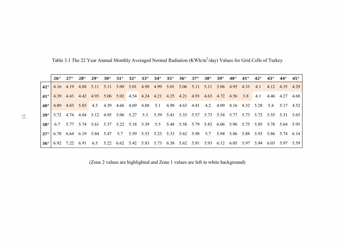
55
Table 3.1 The 22 Year Annual Monthly Averaged Normal Radiation (KWh/m2/day) Values for Grid Cells of Turkey
26° 27° 28° 29° 30° 31° 32° 33° 34° 35° 36° 37° 38° 39° 40° 41° 42° 43° 44° 45°
42° 4.16 4.19 4.88 5.11 5.11 5.09 5.01 4.98 4.99 5.01 5.06 5.11 5.11 5.06 4.95 4.33 4.1 4.12 4.35 4.29
41° 4.39 4.43 4.42 4.93 5.06 5.02 4.54 4.24 4.21 4.25 4.21 4.93 4.63 4.72 4.56 3.8 4.1 4.46 4.27 4.68
40° 4.89 4.83 5.03 4.5 4.39 4.66 4.69 4.88 5.1 4.98 4.63 4.41 4.2 4.09 4.16 4.32 5.28 5.4 5.17 4.52
39° 5.72 4.74 4.84 5.12 4.95 5.06 5.27 5.3 5.39 5.41 5.33 5.57 5.73 5.54 5.77 5.73 5.72 5.55 5.31 5.65
38° 6.7 5.77 5.74 5.61 5.37 5.22 5.18 5.39 5.5 5.48 5.58 5.79 5.82 6.06 5.96 5.75 5.85 5.78 5.64 5.95
37° 6.78 6.64 6.19 5.84 5.47 5.7 5.59 5.53 5.23 5.33 5.62 5.98 5.7 5.94 5.86 5.88 5.93 5.86 5.74 6.14
36° 6.92 7.22 6.91 6.5 5.22 6.62 5.42 5.83 5.73 6.38 5.62 5.91 5.93 6.12 6.05 5.97 5.94 6.03 5.97 5.59
(Zone 2 values are highlighted and Zone 1 values are left in white background)
55
.

56
The observed values are the averages of the SSE values for each zone, shown above;
and the predicted values are calculated as the average radiation amount in USA Solar
Radiation maps corresponding to thermal gradient zones in AASHTO which are
chosen as appropriate for the zones of Turkey.
The comparison of the averages of predicted radiation values of each zone with the
observed values are presented as in Table 3.2
In the table,
Absolute error, AE=|𝐻𝑖𝑖 − 𝐻𝑖𝛾|
Standard error, SE= 𝜎√𝑁
Relative percentage error, 𝑅𝑃𝐸 = 𝐻𝑜−𝐻𝑝�̅�
∗ 100
Mean percentage error, MPE=1𝑁∑ �
𝐻𝑖𝑜−𝐻𝑖𝑝𝐻𝑖𝑜
∗ 100�𝑁𝑐=1
Mean bias error, MBE=1𝑁∑ �𝐻𝑐𝑖 − 𝐻𝑐𝑝�𝑁𝑐=1
Root mean square error, 𝑅𝑀𝑅𝐸 = �1𝑁∑ �𝐻𝑐𝑝 − 𝐻𝑐𝑖�
2𝑁𝑐=1
Here Hio is the ith observed value, Hip is the ith predicted value, N is number of
observations and 𝜎2 is variance.
Mean percentage error can be defined as the deviation of anticipated monthly
average irradiation values from the observed ones. The MBE, expressed as either a
percentage or an absolute value, reveals whether a given model has a t endency to
under- or over-predict. MBE values closest to zero are desirable. The RMSE
indicates the level of dispersion that a model has, thus providing a term-by-term
comparison and show the departure between the predicted and observed values. The
lower RMSE values reflect a b etter model in terms of its absolute deviation.
According to Lingamguna et al. (2004) relative percentage error, RPE smaller than
25% is desired for a model to be acceptable.
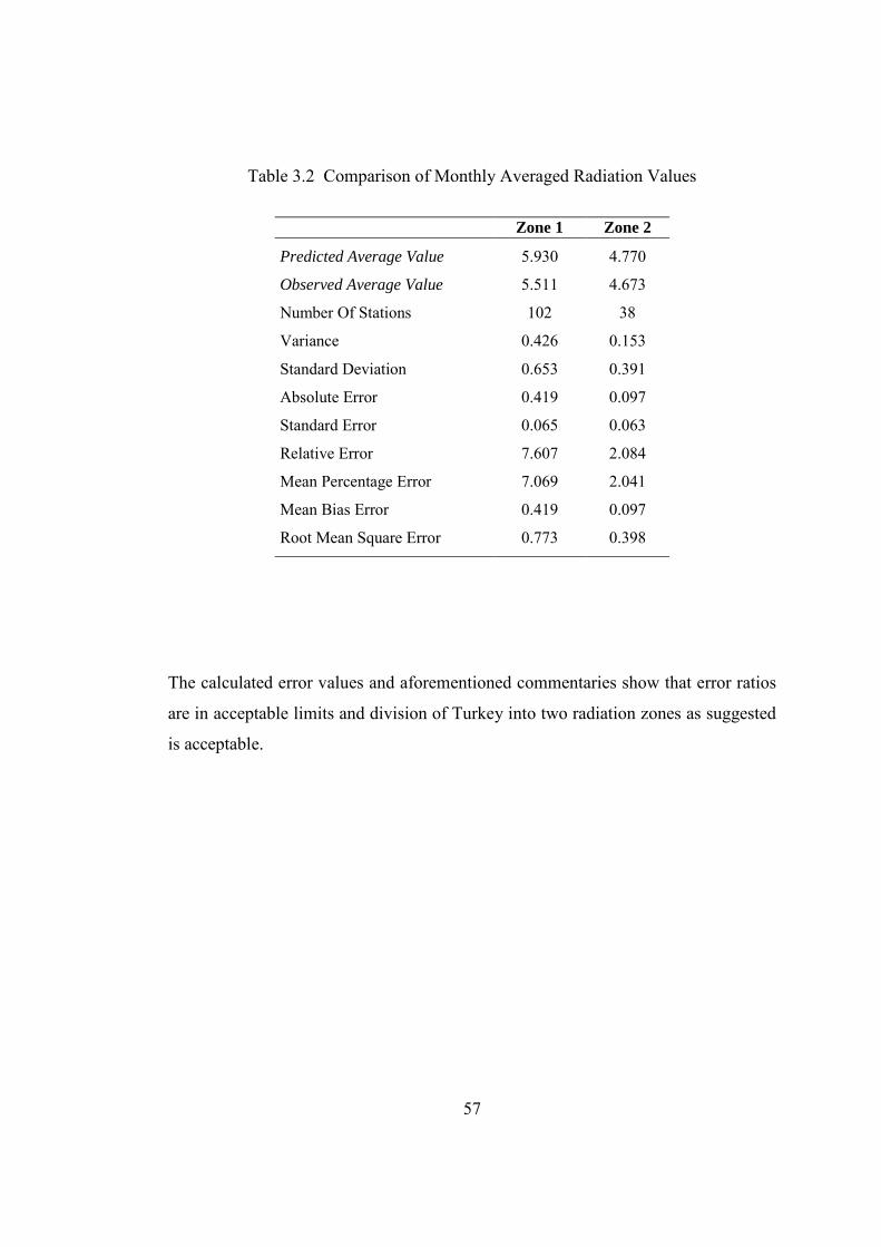
57
Table 3.2 Comparison of Monthly Averaged Radiation Values
Zone 1 Zone 2
Predicted Average Value 5.930 4.770
Observed Average Value 5.511 4.673
Number Of Stations 102 38
Variance 0.426 0.153
Standard Deviation 0.653 0.391
Absolute Error 0.419 0.097
Standard Error 0.065 0.063
Relative Error 7.607 2.084
Mean Percentage Error 7.069 2.041
Mean Bias Error 0.419 0.097
Root Mean Square Error 0.773 0.398
The calculated error values and aforementioned commentaries show that error ratios
are in acceptable limits and division of Turkey into two radiation zones as suggested
is acceptable.

58
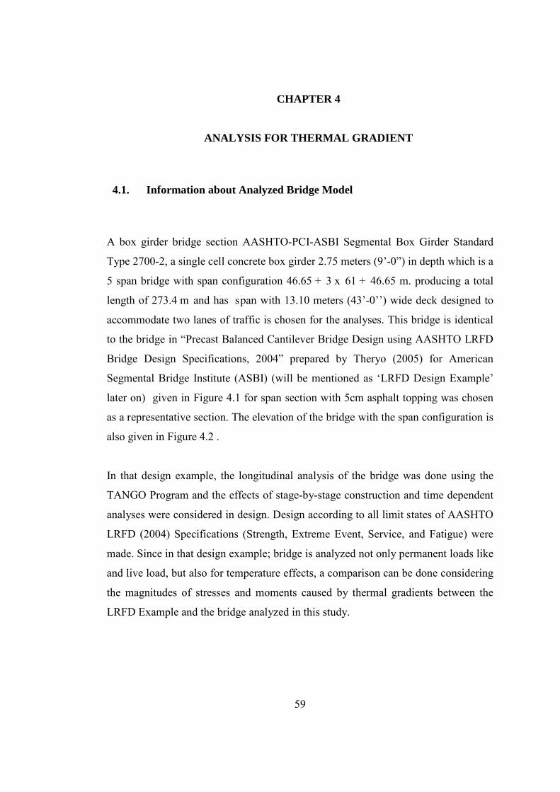
59
CHAPTER 4
4. ANALYSIS FOR THERMAL GRADIENT 4.1. Information about Analyzed Bridge Model
A box girder bridge section AASHTO-PCI-ASBI Segmental Box Girder Standard
Type 2700-2, a single cell concrete box girder 2.75 meters (9’-0”) in depth which is a
5 span bridge with span configuration 46.65 + 3 x 61 + 46.65 m. producing a total
length of 273.4 m and has span with 13.10 meters (43’-0’’) wide deck designed to
accommodate two lanes of traffic is chosen for the analyses. This bridge is identical
to the bridge in “Precast Balanced Cantilever Bridge Design using AASHTO LRFD
Bridge Design Specifications, 2004” prepared by Theryo (2005) for American
Segmental Bridge Institute (ASBI) (will be mentioned as ‘LRFD Design Example’
later on) given in Figure 4.1 for span section with 5cm asphalt topping was chosen
as a representative section. The elevation of the bridge with the span configuration is
also given in Figure 4.2 .
In that design example, the longitudinal analysis of the bridge was done using the
TANGO Program and the effects of stage-by-stage construction and time dependent
analyses were considered in design. Design according to all limit states of AASHTO
LRFD (2004) Specifications (Strength, Extreme Event, Service, and Fatigue) were
made. Since in that design example; bridge is analyzed not only permanent loads like
and live load, but also for temperature effects, a comparison can be done considering
the magnitudes of stresses and moments caused by thermal gradients between the
LRFD Example and the bridge analyzed in this study.

60
Figure 4.1 Bridge girder cross section used in the analysis with its dimensions in mm
Figure 4.2 Elevation view of the bridge (Adopted from Theryo, 2005)
In the aforementioned example, the bridge is analyzed with AASHTO 3rd solar zone
thermal gradient values. For the scope of this research, the cross section is modeled
in a two dimensional (2D) finite element heat transfer analyses program (Figure 4.3):
Panthalassa, developed by Albostan (2013) in Middle East Technical University
laboratories, and sensitivity analyses are were performed for the cross section.
1460150043020801080
230 R200
R410
1
2.5
480
890
230250
2500
10805470
35102290 (2) 3650 lanes = 7300
13100
2500
5000
2740
410
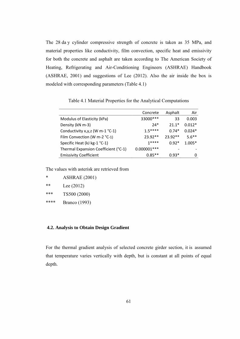
61
The 28 da y cylinder compressive strength of concrete is taken as 35 MPa, and
material properties like conductivity, film convection, specific heat and emissivity
for both the concrete and asphalt are taken according to The American Society of
Heating, Refrigerating and Air-Conditioning Engineers (ASHRAE) Handbook
(ASHRAE, 2001) and suggestions of Lee (2012). Also the air inside the box is
modeled with corresponding parameters (Table 4.1)
Table 4.1 Material Properties for the Analytical Computations
Concrete Asphalt Air Modulus of Elasticity (kPa) 33000*** 33 0.003 Density (kN m-3) 24* 21.1* 0.012* Conductivity x,y,z (W m-1 °C-1) 1.5**** 0.74* 0.024* Film Convection (W m-2 °C-1) 23.92** 23.92** 5.6** Specific Heat (kJ kg-1 °C-1) 1**** 0.92* 1.005* Thermal Expansion Coefficient (°C-1) 0.000001*** - - Emissivity Coefficient 0.85** 0.93* 0
The values with asterisk are retrieved from
* ASHRAE (2001)
** Lee (2012)
*** TS500 (2000)
**** Branco (1993)
4.2. Analysis to Obtain Design Gradient
For the thermal gradient analysis of selected concrete girder section, it is assumed
that temperature varies vertically with depth, but is constant at all points of equal
depth.
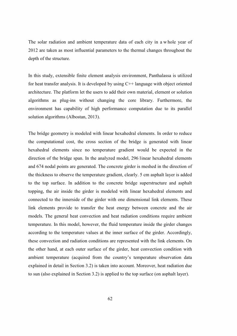
62
The solar radiation and ambient temperature data of each city in a w hole year of
2012 are taken as most influential parameters to the thermal changes throughout the
depth of the structure.
In this study, extensible finite element analysis environment, Panthalassa is utilized
for heat transfer analysis. It is developed by using C++ language with object oriented
architecture. The platform let the users to add their own material, element or solution
algorithms as plug-ins without changing the core library. Furthermore, the
environment has capability of high performance computation due to its parallel
solution algorithms (Albostan, 2013).
The bridge geometry is modeled with linear hexahedral elements. In order to reduce
the computational cost, the cross section of the bridge is generated with linear
hexahedral elements since no temperature gradient would be expected in the
direction of the bridge span. In the analyzed model, 296 linear hexahedral elements
and 674 nodal points are generated. The concrete girder is meshed in the direction of
the thickness to observe the temperature gradient, clearly. 5 cm asphalt layer is added
to the top surface. In addition to the concrete bridge superstructure and asphalt
topping, the air inside the girder is modeled with linear hexahedral elements and
connected to the innerside of the girder with one dimensional link elements. These
link elements provide to transfer the heat energy between concrete and the air
models. The general heat convection and heat radiation conditions require ambient
temperature. In this model, however, the fluid temperature inside the girder changes
according to the temperature values at the inner surface of the girder. Accordingly,
these convection and radiation conditions are represented with the link elements. On
the other hand, at each outer surface of the girder, heat convection condition with
ambient temperature (acquired from the country’s temperature observation data
explained in detail in Section 3.2) is taken into account. Moreover, heat radiation due
to sun (also explained in Section 3.2) is applied to the top surface (on asphalt layer).

63
Since heat radiation data obtained from the data source is as energy rate, it is defined
as surface flux on the asphalt layer. On the other hand, heat radiation between outer
air layer and outside surface of the girder is defined as heat radiation boundary
condition.
Transient heat transfer analyses are performed by utilizing high performance
computer. Analyses are made for the each city in order to give hourly temperature
results for the whole year 2012 f or each node of the section. A high performance
computer that has the properties presented in Table 4.2 is used in the analyses, and
with the provided computer, each analysis took approximately 8 hours (for the output
frequency mentioned in the following paragraph).
Table 4.2. Properties Of The Computer Used In Heat Transfer Analysis Processors Intel Xenon E5630 2.53 GHz
Number of Cores 8
RAM 24 GB
Operating System 64 bit
Readings are obtained for a line along one of the webs in vertical direction from the
topmost of the girder to the base (shown with the red line in Figure 4.3) and an
example visualization of an output for a selected time is given in Figure 4.4. The
initial temperature conditions are taken into account by starting the analysis with data
of the prior month, i.e. December 2011. Results are acquired in hourly intervals in
order not to omit the most critical gradient values. After the analysis the temperature
of each node in cross section is used to calculate the thermal gradient. The highest
positive gradient values tend to occur at 12 p.m. Greenwich Mean Time (2 p.m. for
GMT +2 and 3 p.m. for GMT +3 time zones) in July while negative gradient values
tend to occur at midnight times in December.

64
Figure 4.3 Finite element model of the girder and the line along which the readings are taken
Figure 4.4 An example Panthalassa output visualization for 23.03.12, 2p.m.(GMT+2)

65
The 5 most critical positive gradient values are plotted along the depth of the girder
for one example city from each proposed thermal zone, Ankara from Zone 1 a nd
Istanbul from Zone 2 drawn together in Figures 4.5 and 4.6 with the relevant
AASHTO Solar radiation zones and the zones which are recommended from their
means. (The decision criteria for the selection of proposed gradient values for Turkey
are explained in the following paragraphs). In the following graph, the highest
positive gradient values for each city analyzed are also plotted (Figure 4.7).
Generally T3 values, the temperature gradient values at the bottom of the section are
so small that, they may be ignored in the design. AASHTO (1999 and subsequent)
also allows omitting T3 in design unless a site-specific analysis is made.

66
Figure 4.5 Maximum measured positive gradients (a) and negative gradients (b) in Ankara compared to recommended AASHTO Zone 1 and Turkey Zone 1.
0
500
1000
1500
2000
2500
0 5 10 15 20 25 30 35
Dept
h (m
m)
Temperature (°C)
05.06.2012
14.07.2012
13.07.2012
03.07.2012
12.07.2012
AASHTO Zone 1
Turkey Zone 1
0
500
1000
1500
2000
2500
-7.5 -2.5 2.5
Dept
h (m
m)
Temperature (°C)
15.08.2012
05.10.2012
16.01.2012
20.04.2012
22.04.2012
AASHTO Zone 1
Turkey Zone 1
(a)
(b)

67
Figure 4.6 Maximum measured positive gradients (a) and negative gradients (b) in İstanbul compared to recommended AASHTO Zone 2 and Turkey Zone 2.
0
500
1000
1500
2000
2500
3000
0 5 10 15 20 25 30
Dept
h (m
m)
Temperature (°C)
14.07.2012
24.07.2012
09.07.2012
30.07.2012
15.07.2012
AASHTO Zone 2
Turkey Zone 2
0
500
1000
1500
2000
2500
3000
-7.5 -2.5 2.5 7.5
Dept
h (m
m)
Temperature (°C)
04.12.2012
26.01.2012
05.02.2014
14.12.2012
19.11.2012
AASHTO Zone 2
Turkey Zone 2
(a)
(b)

68
Figure 4.7 Maximum measured positive gradients for 16 city analyzed for Zone 1 (a) and Zone 2 (b) compared to recommended AASHTO and Turkey Zone 1 and 2.
The general tendency for the largest gradient values is similar for all of the analyzed
cities. The highest positive gradients of the days correspond to 3hours after mid-day
3p.m. as a result of the heat and radiation accumulation and the negative gradient
values are the most severe at the 3 a.m. in most days, just before the rise of the sun.
Figure 4.8 shows hourly changing gradient values for two example days for the most
severe positive and negative gradient days of Ankara from Zone 1, Figure 4.9 shows
the same daily changes for Istanbul from Zone 2.
0
500
1000
1500
2000
2500
0 5 10 15 20 25 30 35
Dept
h (m
m)
Temperature (°C)
Adana
Ankara
Antalya
Bingöl
Erzurum
Gaziantep
İzmir
Mugla
Kars
Van
AASHTO Zone 1
Turkey Zone 1
(a)
0
500
1000
1500
2000
2500
0 5 10 15 20 25 30 35
Dept
h (m
m)
Temperature (°C)
Bursa
Çanakkale
Edirne
İstanbul
Samsun
Trabzon
AASHTOZone 2
Turkey Zone2
(b)

69
Figure 4.8 T1 value for Ankara from Zone 1 for the day with highest positive
gradient 05.06.2012 (a) and for the day which the most severe negative gradient
occurs, 15.08.2012 (b)
0
5
10
15
20
25
30
1.00
2.00
3.00
4.00
5.00
6.00
7.00
8.00
9.00
10.0
011
.00
12.0
013
.00
14.0
015
.00
16.0
017
.00
18.0
019
.00
20.0
021
.00
22.0
023
.00
24.0
0
Gra
dien
t Val
ue, T
1 (°C
)
Hour
-4
-2
0
2
4
6
8
10
12
14
1.00
2.00
3.00
4.00
5.00
6.00
7.00
8.00
9.00
10.0
011
.00
12.0
013
.00
14.0
015
.00
16.0
017
.00
18.0
019
.00
20.0
021
.00
22.0
023
.00
24.0
0
Gra
dien
t Val
ue, T
1 (°C
)
Hour
(a)
(b)
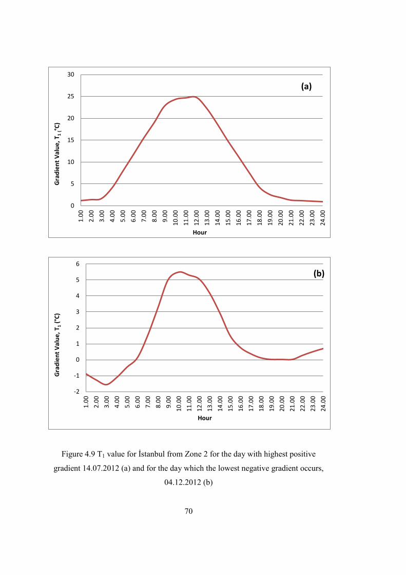
70
Figure 4.9 T1 value for İstanbul from Zone 2 for the day with highest positive
gradient 14.07.2012 (a) and for the day which the lowest negative gradient occurs,
04.12.2012 (b)
0
5
10
15
20
25
301.
002.
003.
004.
005.
006.
007.
008.
009.
0010
.00
11.0
012
.00
13.0
014
.00
15.0
016
.00
17.0
018
.00
19.0
020
.00
21.0
022
.00
23.0
024
.00
Gra
dien
t Val
ue, T
1 (°C
)
Hour
-2
-1
0
1
2
3
4
5
6
1.00
2.00
3.00
4.00
5.00
6.00
7.00
8.00
9.00
10.0
011
.00
12.0
013
.00
14.0
015
.00
16.0
017
.00
18.0
019
.00
20.0
021
.00
22.0
023
.00
24.0
0
Gra
dien
t Val
ue, T
1 (°C
)
Hour
(a)
(b)
71
In Table 4.3, the analyses results showing the maximum temperature differential
between top of concrete girder and average temperature of web for each city are
given. Since the T1 gradient values actually show the temperature difference of top
the deck from the average of webs, T2 as the difference between 10cm below the top
surface and the average of web and, T3 is the difference of the bottom of the girder
from the average of webs, to emphasize that these the values will be given with
“delta” units, and will be referred with Δ°C instead of °C units hereafter.
Table 4.3 Positive and Negative Temperature Gradient Values for the Analyzed Cities
Since the given values are the extreme values for each city; while recommending the
design gradient value, the average of the maximum temperature values of each zone
would be appropriate. According to given analysis results; a 27.3 °C positive
temperature difference for Zone 1 and 24.6 °C for Zone 2 is obtained for T1 as the
averages of the corresponding analyzed locations. Zone maximum extreme T1 values
are 29.5 Δ°C (Gaziantep) and 25.3 Δ °C (Edirne) for Zone 1 and Zone 2 respectively.
Average of the maximum of the gradient values 10cm below the surface, T2 are 5.0
and 6.2 Δ°C for Zone 1 and 2.
T1(max) T2(max) T1(max) T2(max) T1(avg) T2(avg) T1(avg) T2(avg)Adana 27.0 (49.1) 4.5 (8.2) -1.6 (-2.9) -9.8 (-17.8) 4.2 (7.6) 3.2 (5.8) -0.4 (-0.7) -1.7 (-3.1)Ankara 27.1 (49.3) 5.5 (10) -2.4 (-4.4) -4.9 (-8.9) 7.2 (13.1) 5.2 (9.5) -0.3 (-0.5) -1.2 (-2.2)Antalya 26.4 (48.0) 4.3 (7.8) -0.9 (-1.6) -11.1 (-20.2) 6.8 (12.4) 5.1 (9.3) -0.2 (-0.4) -1.2 (-2.2)Bingöl 28.8 (52.4) 6.8 (12.4) -0.8 (-1.5) -3.2 (-5.8) 4.2 (7.6) 3.1 (5.6) -0.2 (-0.4) -1 (-1.8)
Erzurum 24.5 (44.5) 4.6 (8.4) -6.3 (-11.5) -8.7 (-15.8) 3.8 (6.9) 5.2 (9.5) -0.6 (-1.1) -2.5 (-4.5)Gaziantep 29.5 (53.6) 4.5 (8.4) -1.5 (-2.7) -5.7 (-10.4) 4.3 (7.8) 3.1 (5.6) -0.3 (-0.5) -1.5 (-2.7)
İzmir 28.0 (50.9) 5.9 (10.7) -0.9 (-1.6) -7.2 (-13.1) 4.2 (7.6) 3.5 (6.4) -0.2 (-0.4) -1.5 (-2.7)Kars 26.8 (48.7) 3.3 (6.0) -5.7 (-10.4) -8.4 (-15.3) 3.3 (6) 4.1 (7.5) -0.6 (-1.1) -2 (-3.6)
Muğla 28.5 (51.8) 5.7 (10.4) -1.1 (-2.0) -7.9 (-14.4) 4.2 (7.6) 3.1 (5.6) -0.3 (-0.5) -1.3 (-2.4)Van 26.3 (47.8) 5.1 (9.3) -2.0 (-3.6) -3 (-5.5) 4.3 (7.8) 3.4 (6.2) -0.3 (-0.5) -1 (-1.8)
Bursa 24.9 (45.3) 4.4 (8.0) -2.0 (-3.6) -7.2 (-13.1) 3.1 (5.6) 3 (5.5) -0.3 (-0.5) -2.1 (-3.8)Çanakkale 26.1 (47.5) 9.5 (17.3) -1.1 (-2.0) -7.1 (-12.9) 3.3 (6) 3.1 (5.6) -0.2 (-0.4) -1.5 (-2.7)
Edirne 25.3 (47.5) 7.6 (13.8) -0.9 (-1.6) -6.4 (-11.6) 2.8 (5.1) 2.7 (4.9) -0.2 (-0.4) -1.6 (-2.9)İstanbul 24.7 (44.9) 6.2 (11.3) -1.5 (-2.7) -5.4 (-9.8) 2.7 (4.9) 2.5 (4.5) -0.2 (-0.4) -1.3 (-2.4)Samsun 23.1 (42.0) 3.4 (6.2) -1.1 (-2.0) -6.8 (-12.4) 3.3 (6) 3.1 (5.6) -0.3 (-0.5) -2 (-3.6)Trabzon 24.1 (43.8) 6.1 (11.1) -1.0 (-1.8) -4.7 (-8.5) 2.9 (5.3) 2.7 (4.9) -0.1 (-0.2) -1.8 (-3.3)
Positive Temperature Gradient, Δ°C
(
Negative Temperature
Gradient, Δ°C (Δ°F)
Zone 1
Zone 2
Zone City
Positive Temperature
Gradient, Δ°C (Δ°F)
Negative Temperature Gradient, Δ°C (Δ°F)
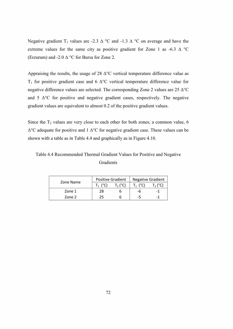
72
Negative gradient T1 values are -2.3 Δ °C and -1.3 Δ °C on average and have the
extreme values for the same city as positive gradient for Zone 1 as -6.3 Δ °C
(Erzurum) and -2.0 Δ °C for Bursa for Zone 2.
Appraising the results, the usage of 28 Δ°C vertical temperature difference value as
T1 for positive gradient case and 6 Δ°C vertical temperature difference value for
negative difference values are selected. The corresponding Zone 2 values are 25 Δ°C
and 5 Δ°C for positive and negative gradient cases, respectively. The negative
gradient values are equivalent to almost 0.2 of the positive gradient values.
Since the T2 values are very close to each other for both zones, a common value, 6
Δ°C adequate for positive and 1 Δ°C for negative gradient case. These values can be
shown with a table as in Table 4.4 and graphically as in Figure 4.10.
Table 4.4 Recommended Thermal Gradient Values for Positive and Negative
Gradients
Zone Name Positive Gradient Negative Gradient T1 (°C) T2 (°C) T1 (°C) T2 (°C)
Zone 1 28 6 -6 -1 Zone 2 25 6 -5 -1
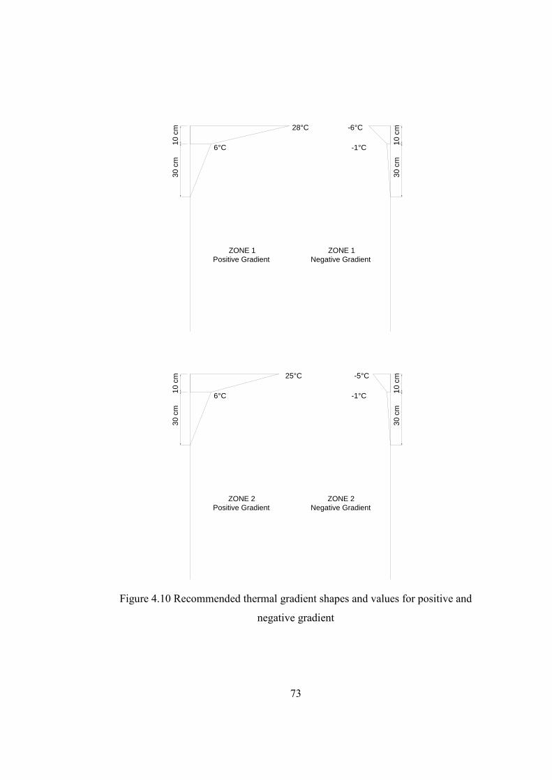
73
Figure 4.10 Recommended thermal gradient shapes and values for positive and
negative gradient
28°C
6°C10 c
m30
cm
-6°C
-1°C 10 c
m30
cm
25°C
6°C10 c
m30
cm
-5°C
-1°C 10 c
m30
cm
ZONE 1Positive Gradient
ZONE 1Negative Gradient
ZONE 2Positive Gradient
ZONE 2Negative Gradient
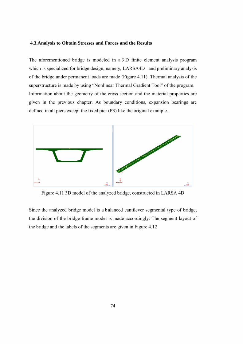
74
4.3.Analysis to Obtain Stresses and Forces and the Results The aforementioned bridge is modeled in a 3 D finite element analysis program
which is specialized for bridge design, namely, LARSA4D and preliminary analysis
of the bridge under permanent loads are made (Figure 4.11). Thermal analysis of the
superstructure is made by using “Nonlinear Thermal Gradient Tool” of the program.
Information about the geometry of the cross section and the material properties are
given in the previous chapter. As boundary conditions, expansion bearings are
defined in all piers except the fixed pier (P3) like the original example.
Figure 4.11 3D model of the analyzed bridge, constructed in LARSA 4D
Since the analyzed bridge model is a balanced cantilever segmental type of bridge,
the division of the bridge frame model is made accordingly. The segment layout of
the bridge and the labels of the segments are given in Figure 4.12
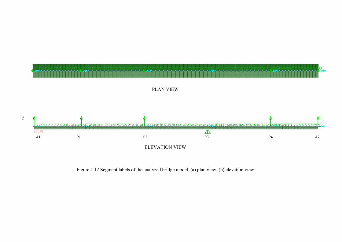
75
PLAN VIEW
ELEVATION VIEW
Figure 4.12 Segment labels of the analyzed bridge model, (a) plan view, (b) elevation view
A1 P1 P2 P3 P4 A2
75
.
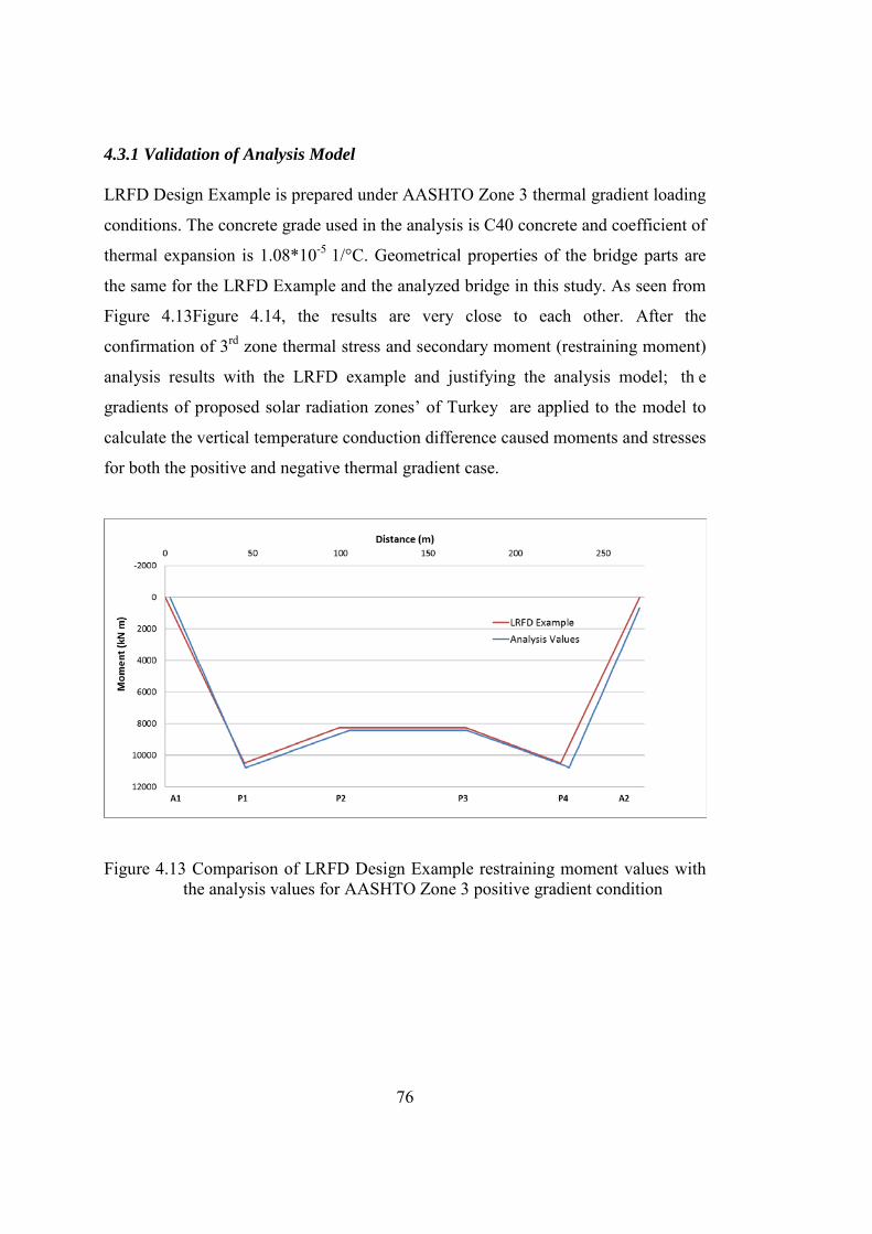
76
4.3.1 Validation of Analysis Model LRFD Design Example is prepared under AASHTO Zone 3 thermal gradient loading
conditions. The concrete grade used in the analysis is C40 concrete and coefficient of
thermal expansion is 1.08*10-5 1/°C. Geometrical properties of the bridge parts are
the same for the LRFD Example and the analyzed bridge in this study. As seen from
Figure 4.13Figure 4.14, the results are very close to each other. After the
confirmation of 3rd zone thermal stress and secondary moment (restraining moment)
analysis results with the LRFD example and justifying the analysis model; th e
gradients of proposed solar radiation zones’ of Turkey are applied to the model to
calculate the vertical temperature conduction difference caused moments and stresses
for both the positive and negative thermal gradient case.
Figure 4.13 Comparison of LRFD Design Example restraining moment values with the analysis values for AASHTO Zone 3 positive gradient condition
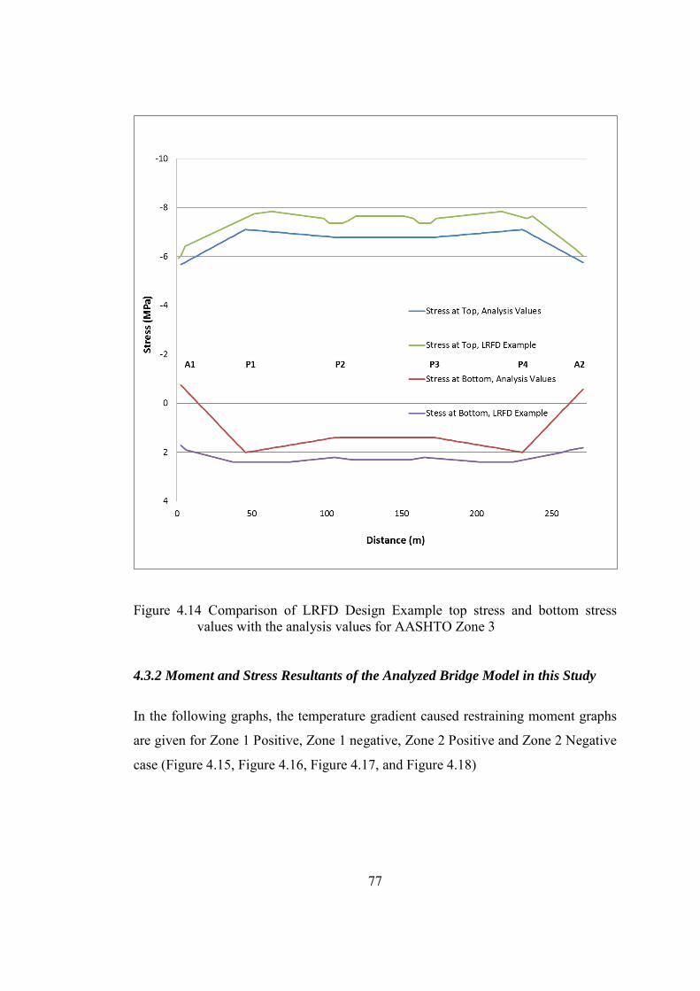
77
Figure 4.14 Comparison of LRFD Design Example top stress and bottom stress values with the analysis values for AASHTO Zone 3
4.3.2 Moment and Stress Resultants of the Analyzed Bridge Model in this Study
In the following graphs, the temperature gradient caused restraining moment graphs
are given for Zone 1 Positive, Zone 1 negative, Zone 2 Positive and Zone 2 Negative
case (Figure 4.15, Figure 4.16, Figure 4.17, and Figure 4.18)

78
Figure 4.15 Non-linear positive temperature gradient restraining moments for Zone 1
Figure 4.16 Non-linear negative temperature gradient restraining moments for Zone 1

79
Figure 4.17 Non-linear positive temperature gradient restraining moments for Zone 2
Figure 4.18 Non-linear negative temperature gradient restraining moments for Zone 2 The most critical thermal stress values are developed at the 17th and 65th segments
with similar results (the detailed segment layout was given in Figure 4.12 before).
The detailed cross section stresses for recommended Zone 1 pos itive, Zone 1
negative, Zone 2 positive and Zone 2 are given in the Figures 4.19, 4.20, 4.21, and
4.22 respectively (compression is shown in negative and tension is shown in positive
in all graphs).
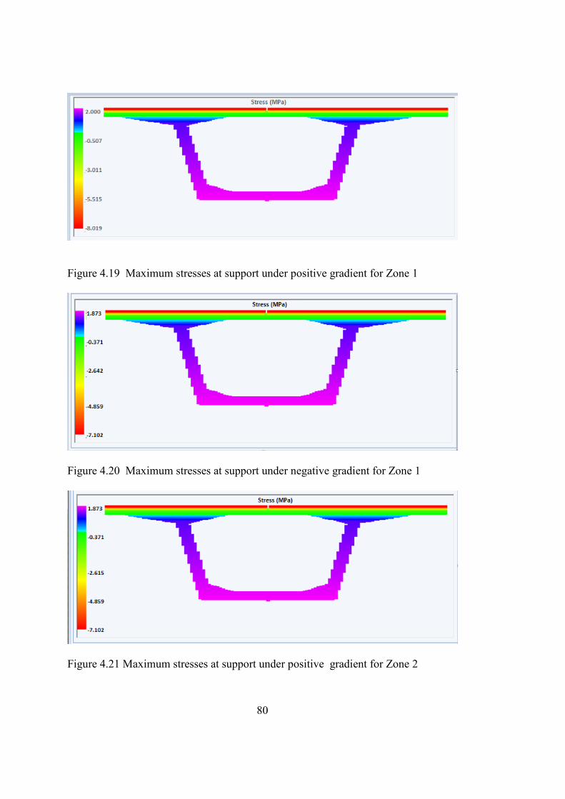
80
Figure 4.19 Maximum stresses at support under positive gradient for Zone 1
Figure 4.20 Maximum stresses at support under negative gradient for Zone 1
Figure 4.21 Maximum stresses at support under positive gradient for Zone 2
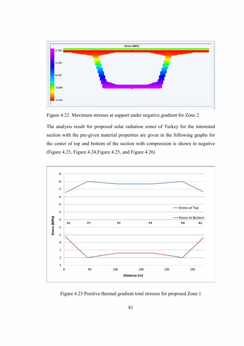
81
Figure 4.22 Maximum stresses at support under negative gradient for Zone 2 The analysis result for proposed solar radiation zones of Turkey for the interested
section with the pre-given material properties are given in the following graphs for
the center of top and bottom of the section with compression is shown in negative
(Figure 4.23, Figure 4.24,Figure 4.25, and Figure 4.26)
Figure 4.23 Positive thermal gradient total stresses for proposed Zone 1
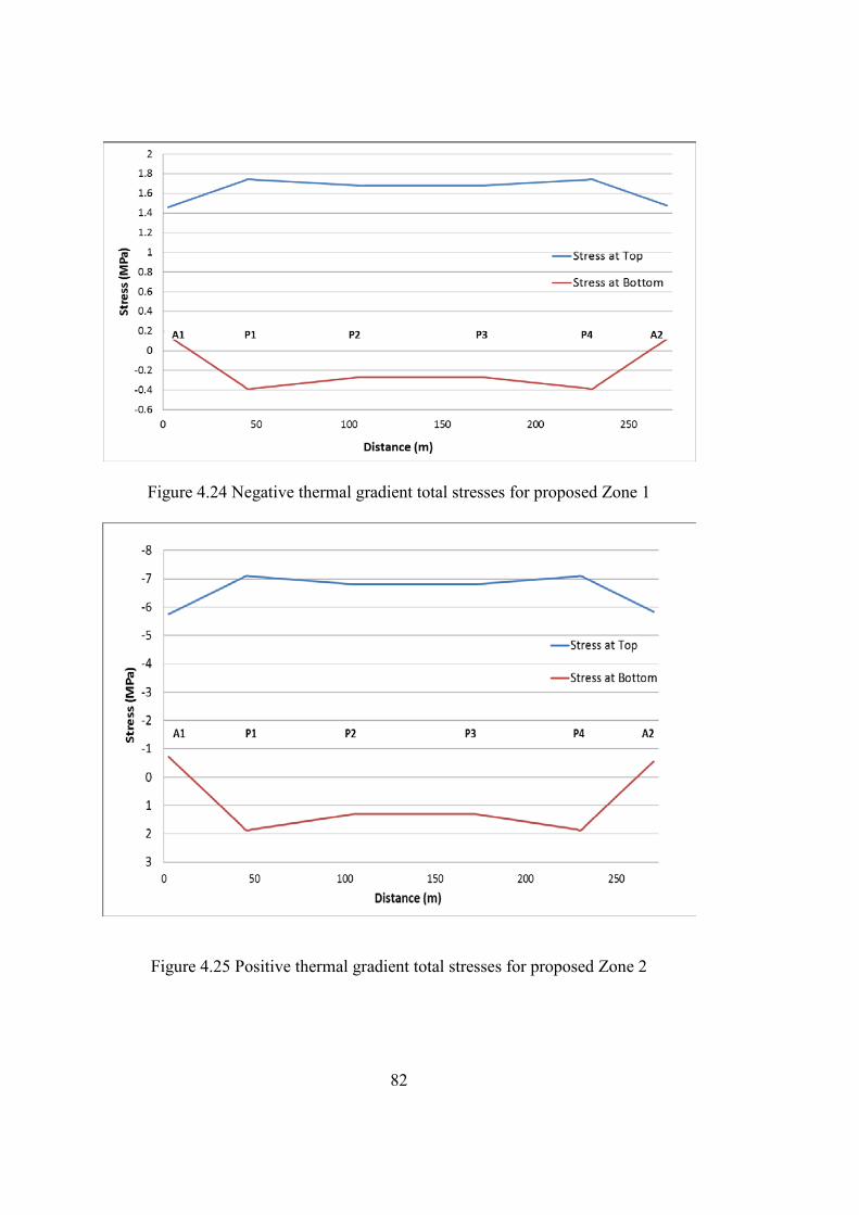
82
Figure 4.24 Negative thermal gradient total stresses for proposed Zone 1
Figure 4.25 Positive thermal gradient total stresses for proposed Zone 2

83
Figure 4.26 Negative thermal gradient total stresses for proposed Zone 2 In addition to C35, the same section is also analyzed for positive thermal gradient for
different concrete grades, C40 and C45 which are commonly used in post-tensioned
segmental bridges in order to see the effect of material grade to thermal gradient
originated stresses. The positive gradient analysis results for different kinds of
materials is shown in the following figures (Figure 4.27 and Figure 4.28)

84
Figure 4.27 Top stress values for different concrete grades caused by positive gradient of Zone 1
Figure 4.28 Bottom stress values for different concrete grades caused by positive
gradient of Zone 1

85
As can be seen from the above figures, the change in the concrete material grade
does not affect the highest stress values much. The stress values get higher as the
grade increases since the elasticity modulus is increasing.
As mentioned in the section 3.3.2 , according to AASHTO (2012), the allowable
stress limits for concrete is investigated for two time intervals of construction
schedule, temporary stresses before the losses due to creep and shrinkage before the
appliance of prestress and stresses at service limit state after prestress losses. The
maximum compression and tension limits for the analyzed segmental bridge
structure with the material used in the analysis, C35 concrete is tabulated in Table
4.5.
Table 4.5 Allowable compression and tension stresses for C35 concrete for thermal gradient analysis of a segmental bridge top section according to AASHTO (2012)
Time Interval Compressive
Stress (MPa)
Tension
Stress (MPa)
Before prestress 15.8 3.7
After prestress 15.8 1.5
As seen from Figure 4.19 and Figure 4.21, the highest compressive stresses for the
analyzed section are 8.0 and 7.0 M Pa for Zone 1 a nd Zone 2 r espectively. The
highest negative stress values are 2.0 and 1.9 MPa as can be seen from Figure 4.20
and Figure 4.22 The compressive stress values are all below the allowable
compression limits, whereas, the tensile stress limits for C35 are exceeded for Zone 1
negative gradient case and very close to the limit for Zone 2 negative gradient case.
The results show that, in addition to the one done for dead and live loads, additional
prestressing is necessary to overcome these temperature gradient originated stresses.
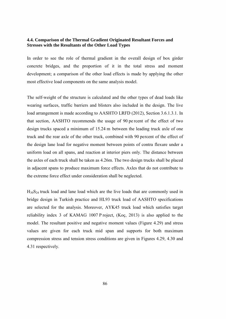
86
4.4. Comparison of the Thermal Gradient Originated Resultant Forces and Stresses with the Resultants of the Other Load Types
In order to see the role of thermal gradient in the overall design of box girder
concrete bridges, and the proportion of it in the total stress and moment
development; a comparison of the other load effects is made by applying the other
most effective load components on the same analysis model.
The self-weight of the structure is calculated and the other types of dead loads like
wearing surfaces, traffic barriers and blisters also included in the design. The live
load arrangement is made according to AASHTO LRFD (2012), Section 3.6.1.3.1. In
that section, AASHTO recommends the usage of 90 pe rcent of the effect of two
design trucks spaced a minimum of 15.24 m between the leading truck axle of one
truck and the rear axle of the other truck, combined with 90 percent of the effect of
the design lane load for negative moment between points of contra flexure under a
uniform load on all spans, and reaction at interior piers only. The distance between
the axles of each truck shall be taken as 4.26m. The two design trucks shall be placed
in adjacent spans to produce maximum force effects. Axles that do not contribute to
the extreme force effect under consideration shall be neglected.
H30S24 truck load and lane load which are the live loads that are commonly used in
bridge design in Turkish practice and HL93 truck load of AASHTO specifications
are selected for the analysis. Moreover, AYK45 truck load which satisfies target
reliability index 3 of KAMAG 1007 P roject, (Koç, 2013) is also applied to the
model. The resultant positive and negative moment values (Figure 4.29) and stress
values are given for each truck mid span and supports for both maximum
compression stress and tension stress conditions are given in Figures 4.29, 4.30 and
4.31 respectively.

87
Figure 4.29 Positive and negative moment values for various truck loads
Figure 4.30 Maximum and minimum truck stresses for mid-span
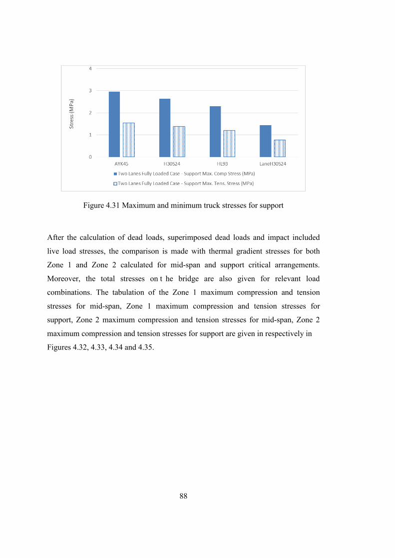
88
Figure 4.31 Maximum and minimum truck stresses for support
After the calculation of dead loads, superimposed dead loads and impact included
live load stresses, the comparison is made with thermal gradient stresses for both
Zone 1 and Zone 2 calculated for mid-span and support critical arrangements.
Moreover, the total stresses on t he bridge are also given for relevant load
combinations. The tabulation of the Zone 1 maximum compression and tension
stresses for mid-span, Zone 1 maximum compression and tension stresses for
support, Zone 2 maximum compression and tension stresses for mid-span, Zone 2
maximum compression and tension stresses for support are given in respectively in
Figures 4.32, 4.33, 4.34 and 4.35.
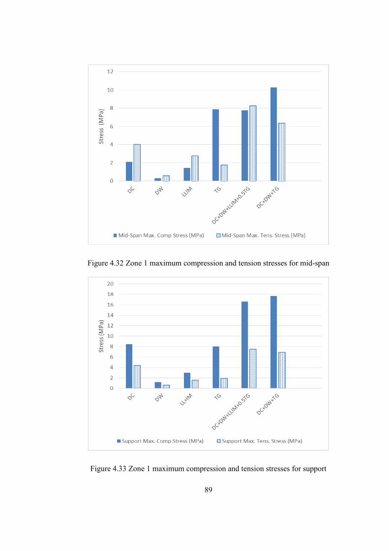
89
Figure 4.32 Zone 1 maximum compression and tension stresses for mid-span
Figure 4.33 Zone 1 maximum compression and tension stresses for support

90
Figure 4.34 Zone 2 maximum compression and tension stresses for mid-span
Figure 4.35 Zone 2 maximum compression and tension stresses for support
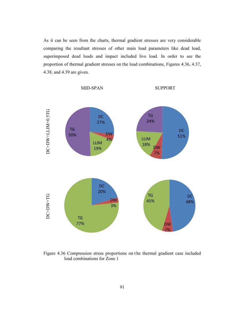
91
As it can be seen from the charts, thermal gradient stresses are very considerable
comparing the resultant stresses of other main load parameters like dead load,
superimposed dead loads and impact included live load. In order to see the
proportion of thermal gradient stresses on the load combinations, Figures 4.36, 4.37,
4.38, and 4.39 are given.
MID-SPAN SUPPORT
DC
+DW
+LLI
M+0
.5TG
DC
+DW
+TG
Figure 4.36 Compression stress proportions on t he thermal gradient case included load combinations for Zone 1
DC 27%
DW 4%
LLIM 19%
TG 50%
DC 51%
DW 7%
LLIM 18%
TG 24%
DC 20%
DW 3%
TG 77%
DC 48%
DW 7%
TG 45%

92
MID-SPAN SUPPORT
DC
+DW
+LLI
M+0
.5TG
DC
+DW
+TG
Figure 4.37 Tension stress proportions on t he thermal gradient case included load combinations for Zone 1
DC 49%
DW 7%
LLIM 33%
TG 11%
DC 58% DW
8%
LLIM 21%
TG 13%
DC 63%
DW 9%
TG 28%
DC 63%
DW 9%
TG 28%
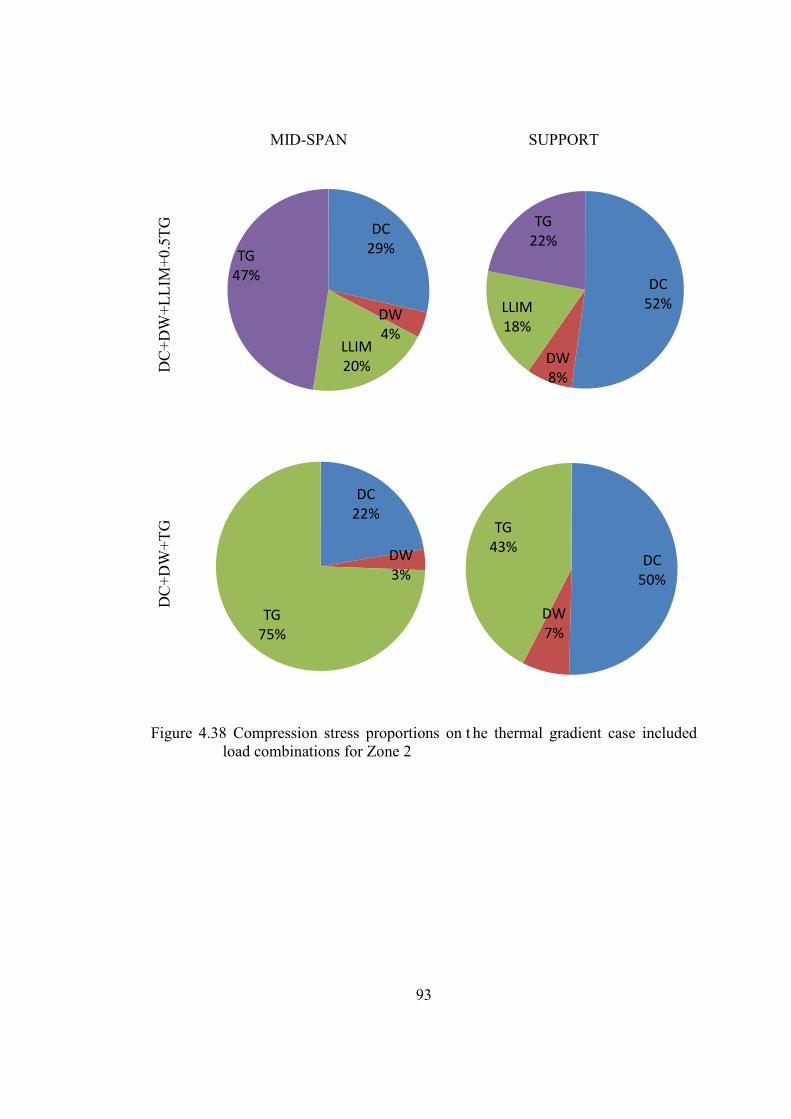
93
MID-SPAN SUPPORT D
C+D
W+L
LIM
+0.5
TG
DC
+DW
+TG
Figure 4.38 Compression stress proportions on t he thermal gradient case included load combinations for Zone 2
DC 29%
DW 4%
LLIM 20%
TG 47% DC
52%
DW 8%
LLIM 18%
TG 22%
DC 22%
DW 3%
TG 75%
DC 50%
DW 7%
TG 43%
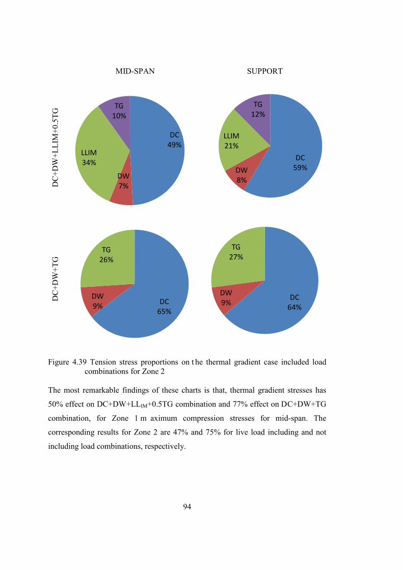
94
MID-SPAN SUPPORT
DC
+DW
+LLI
M+0
.5TG
DC
+DW
+TG
Figure 4.39 Tension stress proportions on t he thermal gradient case included load combinations for Zone 2
The most remarkable findings of these charts is that, thermal gradient stresses has
50% effect on DC+DW+LLIM+0.5TG combination and 77% effect on DC+DW+TG
combination, for Zone 1 m aximum compression stresses for mid-span. The
corresponding results for Zone 2 are 47% and 75% for live load including and not
including load combinations, respectively.
DC 49%
DW 7%
LLIM 34%
TG 10%
DC 59% DW
8%
LLIM 21%
TG 12%
DC 65%
DW 9%
TG 26%
DC 64%
DW 9%
TG 27%

95
Taking into consideration both span and support tensile stress results, for live load
including load combination; for both Zone 1 a nd Zone 2; thermal gradient has
10~13% role, whereas, for non-live load including load combination, that ratio is
26~28%.
As seen from the above charts, thermal gradient has an important role on especially
span stresses for compression stress condition. Gradient results are more critical for
mid-spans than the supports for compressive stresses. For live load including load
combination, thermal gradient results nearly doubles the live load effects.
Also for the combination that does not involve live load; thermal gradient load is far
by the most influencing load parameter for compressive case. For tensile stress case,
mid-span and support results are very close to each other

96

97
CHAPTER 5
5. CONCLUSIONS AND FUTURE WORK
In this study, a solar radiation map for Turkey is constructed and design gradient
shape is recommended for especially box girder bridge design. The corresponding
map and the values for temperature gradients are obtained by analyzing the primary
influencing data for selected 16 cities of the country from the two proposed solar
radiation zones, Zone 1 and Zone 2 for Turkey.
Main findings and conclusions of this study are as follows:
• Two different zones have been identified for Turkey to be used in thermal
gradient loading of concrete box bridges after detailed investigation of local
solar changes at different parts of the country.
• Correctness of analytical bridge model has been achieved through example
bridge results based on AASHTO 3rd Zone.
• At each proposed zone, investigation of thermal gradient induced stresses for
concrete box girder bridges resulted in comparable stresses at different parts
of the same zone based on local solar variations.
• The analyze result value to determine positive gradient T1 value for Zone 2 is
the same as the AASHTO recommendation, and the proposed value for Zone
1 is slightly below t he AASHTO value. Therefore; independent solar
radiation zones for Turkey is suggested and, usage of 28 Δ°C for Zone 1 and
25 Δ°C for Zone 2 for design of bridges for thermal gradient is
recommended.
• It is seen that the temperature difference 10 cm below the top surface,
namely T2 values can be taken as 6 Δ°C for both of the zones.

98
• After 40cm from the top of the section, the temperature values throughout
the depth does not change flagrantly that means the temperature gradient is
zero after 40 cm.
• Since the negative gradient values after the analysis is obtained are quite
smaller than AASHTO recommendations; it will be convenient to use -0.30
times of the positive gradient value for the bridges which have decks of
which top surfaces has asphalt topping less 5cm, and -0.20 times of positive
gradient for the decks which have higher insulating materials as current
AASHTO LRFD Code recommends.
• In this study it is verified that nonlinear temperature distribution developed
through the depth of box girder type bridges can cause bending moments as
high as the ones generated by dead and live loads. Moreover, in terms of
stresses, the obtained values are so high; that, especially for negative gradient
condition, the high tensile forces imposes the requirement of additional
prestressing in order to satisfy tensile stress limitation requirements and
avoid cracking of the section.
For future investigations, the following studies may be done to improve the subject:
• The proposed thermal gradients may be applied on different bridges having
different types of box girder bridges. This difference may be in the depth of
girder, span width and other dimensional properties. Also box girder bridges
having more than one cell may be analyzed.
• A substantial number of segmental box girder bridges have segments whose
girder depth is increasing from mid-span to the supports. In some bridges this
difference is more than two times. Therefore, a b ridge with a v arying
superstructure depth should also be investigated.

99
• A bridge analysis with not only temperature gradient loading, but also other
kinds of load cases like earthquake and wind resultant forces may also be
implemented to compare the effects for other important load factors
governing the bridge design.
• Transverse temperature stresses may also be investigated to find out the
temperature difference between the different webs of the girder and a
transverse temperature gradient may be suggested.

100

101
REFERENCES
Aksoy, B. (1997a). Estimated Monthly Average Global Radiation for Turkey and Its Comparison with Observation. Renewable Energy, 10, 625–633. Aksoy, B. (2011). Solar Radiation over Turkey and Its Analysis. International Journal Of Remote Sensing, 32(21), 6261-6272. Albostan, U. (2013). Implementation of Coupled Thermal and Structural Analysis Methods for Reinforced Concrete Structures (Master Thesis, Middle East Technical University) American Association of State Highway and Transportation Officials (AASHTO). (1989a). Guide Specifications for Design and Construction of Segmental Bridges, Washington, DC. American Association of State Highway and Transportation Officials (AASHTO). (1989b). Guide Specifications: Thermal Effects in Concrete Bridge Superstructures, Washington, DC. American Association of State Highway and Transportation Officials (AASHTO). (1989c). Standard Specifications for Highway Bridges, Washington, D.C. American Association of State Highway and Transportation Officials (AASHTO). (1994b). Interim Specifications for the Guide Specifications for Design and Construction of Segmental Bridges, Washington, DC. American Association of State Highway and Transportation Officials (AASHTO). (1998a). LRFD Bridge Design Specifications, Washington, D.C. American Association of State Highway and Transportation Officials (AASHTO). (1999). Guide Specifications for Design and Construction of Segmental Bridges, Washington, DC. American Association of State Highway and Transportation Officials (AASHTO). (2002). Standard Specifications for Highway Bridges, Washington, D.C. American Association of State Highway and Transportation Officials (AASHTO). (2012). LRFD Bridge Design Specifications, Washington, D.C. American Society of Heating, Refrigerating and Air-Conditioning Engineers (ASHRAE). (2001). ASHRAE Handbook, Atlanta.
102
Branco, F. A., & Mendes, P. A. (1993). Thermal Actions for Concrete Bridge Design. Journal of Structural Engineering, 119(8), 2313-2331. British Standards Institution (BSI). (1979). Steel, Concrete and Composite Bridges: Part 5: Code of Practice for Design of Composite Bridges. BS 5400, London. Cooke, N., Priestly, M. J. N., & Thurston, S. J. (1984). Analysis and Design of Partially Prestressed Concrete Bridges under Thermal Loading. Prestressed Concrete Institute Journal, 16(6), 338. Elbadry, M. M., & Ghali, A. (1983). Temperature Variations in Concrete Bridges. Journal of Structural Engineering, 109(10), 2355-2374. European Committee for Standardization (CEN). (2003). Eurocode 1: Actions on Structures Part 1-5: General Actions-Thermal Actions. The European Standard BS EN 1991-1-5:2003, Brussels. German Institute for Standardization (DIN). (1967). Strassen and Wegbrucken (Street and Road Bridges). DIN 1072, Ber1in and Koln. Hamilton, H. R., Consolazio, G. R. (2009) Validation of Stresses Caused by Thermal Gradients in Segmental Concrete Construction. Final Report, UF Project No. 00030906. University of Florida Department of Civil and Coastal Engineering. Hoffman, P.C., McClure, R.M., and West, H.H. (1980) Temperature Studies for an Experimental Bridge, Research Project 75-3 Interim Report, Pennsylvania State University. Honório J.D. (2007). Conceptual Design of Long-Span Cantilever Constructed Concrete Bridges (Master Thesis, Royal Institute of Technology (KTH), Sweden). Imbsen, R. A., Vandershaf, D. E., Schamber, R. A., and Nutt, R. V. (1985) Thermal Effects in Concrete Bridge Superstructures. NCHRP Program Report 276, Transportation Research Board, Washington D.C., 63-67. Koç, A. F. (2013). Calibration of Turkish LRFD Bridge Design Method for Slab on Steel Plate Girders. (Master Thesis, Middle East Technical University). Lee, J. H. (2011). Investigation of Extreme Environmental Conditions and Design Thermal Gradients During Construction for Prestressed Concrete Bridge Girders. Journal of Bridge Engineering, 17(3), 547-556.

103
Lee, J. H., & Kalkan, I. (2012). Analysis of Thermal Environmental Effects on Precast, Prestressed Concrete Bridge Girders: Temperature Differentials and Thermal Deformations. Advances in Structural Engineering, 15(3), 447-460. Leonhardt, F., Kolbe, G., Peter, J. (1965) Temperaturunterschiede Gefahrden Spannbetonbrilcke (Temperature Differences Endanger Prestressed Concrete Bridges), Beton und Stahlbetonbau, 60 (7): 231-244. Lingamgunta, C., & Veziroglu, T. N. (2004). A Universal Relationship for Estimating Clear Sky Insolation. Energy Conversion and Management, 45(1), 27-52. National Aeronautics and Space Administration (NASA). Surface Meteorology and Solar Energy: Data subset., http://eosweb.larc.nasa.gov., last visited in January 2014. National Climatic Data Center, National Oceanic and Atmospheric Administration (NOAA). Hourly/Sub-Hourly Observational Data., gis.ncdc.noaa.gov/map/viewer, last visited on January 2014. Post-Tensioning Institute (PTI) and Precast/Prestressed Concrete Institute. (1997). Precast Segmental Box Girder Bridge Manual, Arizona. Potgieter, I. C., & Gamble, W. L. (1983). Response of Highway Bridges to Nonlinear Temperature Distributions. University of Illinois Engineering Experiment Station. College of Engineering. University of Illinois at Urbana-Champaign. Priestley, M. N. (1978). Design of Concrete Bridges for Temperature Gradients. ACI Journal Proceedings, 75(5), 209-217. Roberts, C. L., Breen, J. E., and Kreger, M. E. (1993). Measurement based revisions for segmental bridge design criteria. Research Report, 1234-3F, Center for Transportation Research, Univ. of Texas at Austin. Roberts-Wollman, C. L., Breen, J. E., & Cawrse, J. (2002). Measurements of Thermal Gradients and Their Effects on Segmental Concrete Bridge. Journal of Bridge Engineering, 7(3), 166-174. Schlaich, J., & Scheef, H. (1982). Concrete Box-Girder Bridges (Vol. 1). International Association for Bridge and Structural Engineering, Zurich. Shushkewich, K. W. (1998). Design of Segmental Bridges for Thermal Gradient. PCI Journal, 43(4), 120-137. T.C. Bayındırlık Bakanlığı, Karayolları Genel Müdürlüğü. (1982). Yol Köprüleri için Teknik Şartname, Ankara.

104
The Scientific And Technological Research Council Of Turkey (TUBITAK) (2009-2014) KAMAG 1007, 110G093. Theryo, T.S. (2005). Precast Balanced Cantilever Bridge Design Using AASHTO LRFD Bridge Design Specifications.American Segmental Bridge Institute. Turkish Standards Institute, TS500 (2000). Requirements for Design and Construction of Reinforced Concrete Structures, Ankara. Wood, B. A. (1997). Thermal Gradients and Their Effects on Segmental Concrete Box Girder Bridges (Doctoral Dissertation, The University of Texas at Austin). http://www.cement.org/for-concrete-books-learning/concrete-technology/concrete-design-production/mass-concrete, last visited on December 2014.

105
APPENDIX A
A. NUMERICAL HAND CALCULATION DESIGN EXAMPLE
Thermal stresses are developed because of restraint to expansion and rotation from
the restraints coming from the section itself due to the need of section to stay plane
and the restraints resulting from the support conditions. Cross section cause stresses
that vary in the vertical direction whereas support conditions induce stresses that
change longitudinal direction.
Here is an example given for calculating the primary compressive thermal stresses
developed due to the positive gradient for the mid-span section in LRFD Design
Example (Figure 4.1). The total section depth is constant along the whole length of
the bridge. The only variable, the section bottom flange depth is changing from 23
cm to 46 cm from mid-span sections to the supports. Calculations are made for mid-
span sections since as Shushkewich (1998) indicates, Ttop and Tbot values have larger
values at midspan and smaller values at the support.
Secondary stresses are than can be calculated by a plane frame computer program
using the calculated equivalent temperature gradient values as inputs.
The primary stresses components are the superposition of the thermal stresses f(y),
axial stresses NP/A and the flexural stresses Mp y / I. Secondary stresses also cause
axial stresses Ns/A and additional moments Ms y/I. The total stress is the sum of
these components.
The thermal stress component may be considered as a tensile resultant force PR
applied with eccentricity etop from the top of girder. This resultant force is can be
thought as equal to a primary tensile axial force Np and primary bending moment in
negative direction, Mp, applied at ytop, the distance of taken as distance of the
neutral axis of the section with respect to the top. (Figure A.1)

106
Figure A.1 Equivalent force and stress diagram for positive and negative gradient Here, an example is given for the example bridge section that the necessary
information is given before, with the thermal gradient values suggested for Zone 1.
With the help of the section properties and following formulas the primary force and
moment effects can be calculated. In the following figure, the simplified equivalent
I-section for the example box girder section and the gradient that will be applied is
shown (Figure A.2 and Figure A.3)
Figure A.2 Equivalent I-section for the example box girder section
P
Np
Mp
y top
e top
y

107
Figure A.3 Equivalent section dimensions and the applied gradient
A=7.0856 x106 mm2
I=6.9597 x 1012 mm4
ytop = 0.9256 x103 mm
E= 33000 MPa (C35)
α= 10-5 1/°C
𝑓(𝑦) = 𝐸 𝛼 𝑇𝑇(𝑦) (A.1)
𝑃 = 𝐸 𝛼 ∑ 𝑇𝑇(𝑦)𝑏(𝑦) 𝑑𝑦𝑦 (A.2)
𝑀 = 𝐸 𝛼 ∑ 𝑇𝑇(𝑦)𝑏(𝑦) 𝑦 𝑑𝑦𝑦 (A.3)
If the section top stresses are calculated resulted from the positive and negative
gradient for the topmost fibers of the section for Zone 1, with Equation (A.1),
𝑓(𝑡𝑖𝛾)𝑝 = 𝐸 𝛼 𝑇𝑇(𝑡𝑖𝛾) =33000*0.00001*28 =9.24 MPa
𝑓(𝑡𝑖𝛾)𝑛 = 𝐸 𝛼 𝑇𝑇(𝑡𝑖𝛾) =33000*0.00001*6 =1.98 MPa
100130
170
260
1550
250
230
4160
800
1860
5000
28 C
y (mm)
z
6 C13100
b (mm) T ( C)
50
3.4 C1560

108
Then, resultant axial force P and bending moment M can be calculated by dividing
the section into subsections and summing the results as given in the Table A.A.1 and
Table A.A.2.
Table A.A.1 Positive Temperature Gradient Primary Force Calculations for Zone 1
Section E (MPa) α (1/°C) TG (°C) b (mm) t (mm) P (kN) y (mm) M (kN m) I 33000 0.00001 6 13100 100 2594 50 130
II 33000 0.0000100 11 13100 100 4755 33 157
III 33000 0.0000100 3.4 13100 130 1911 165 315
IV 33000 0.0000100 1.3 13100 130 731 143 105
V 33000 0.0000100 1.7 2860 170 273 287 78
Total 10264 785
Table A.A.2 Negative Temperature Gradient Primary Force Calculations for Zone 1
Section E (MPa) α (1/°C) TG (°C) b (mm) t (mm) P (kN) y (mm) M (kN m) I 33000 0.00001 -1 13100 100 -432 50 -22
II 33000 0.00001 -3.5 13100 100 -1513 33 -50
III 33000 0.00001 -0.6 13100 130 -337 165 -56
IV 33000 0.00001 -0.8 13100 130 -450 143 -64
V 33000 0.00001 -0.3 2860 170 -48 287 -14
Total -2780 -206
𝑒𝑡𝑖𝑝 = 𝑀/𝑃 (A.4)
Using (A.4) etop is calculated as 76.5 mm from the top for the positive gradient.
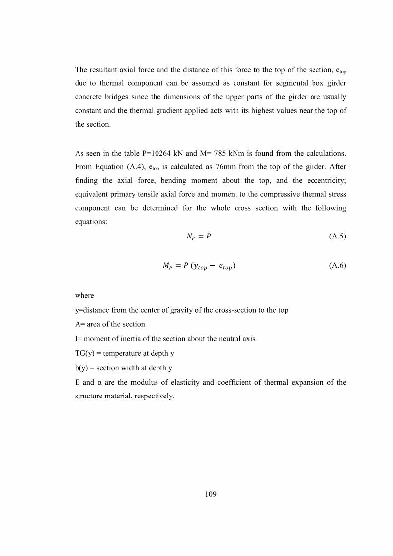
109
The resultant axial force and the distance of this force to the top of the section, etop
due to thermal component can be assumed as constant for segmental box girder
concrete bridges since the dimensions of the upper parts of the girder are usually
constant and the thermal gradient applied acts with its highest values near the top of
the section.
As seen in the table P=10264 kN and M= 785 kNm is found from the calculations.
From Equation (A.4), etop is calculated as 76mm from the top of the girder. After
finding the axial force, bending moment about the top, and the eccentricity;
equivalent primary tensile axial force and moment to the compressive thermal stress
component can be determined for the whole cross section with the following
equations:
𝑁𝑃 = 𝑃 (A.5)
𝑀𝑃 = 𝑃 (𝑦𝑡𝑖𝑝 − 𝑒𝑡𝑖𝑝) (A.6)
where
y=distance from the center of gravity of the cross-section to the top
A= area of the section
I= moment of inertia of the section about the neutral axis
TG(y) = temperature at depth y
b(y) = section width at depth y
E and α are the modulus of elasticity and coefficient of thermal expansion of the
structure material, respectively.
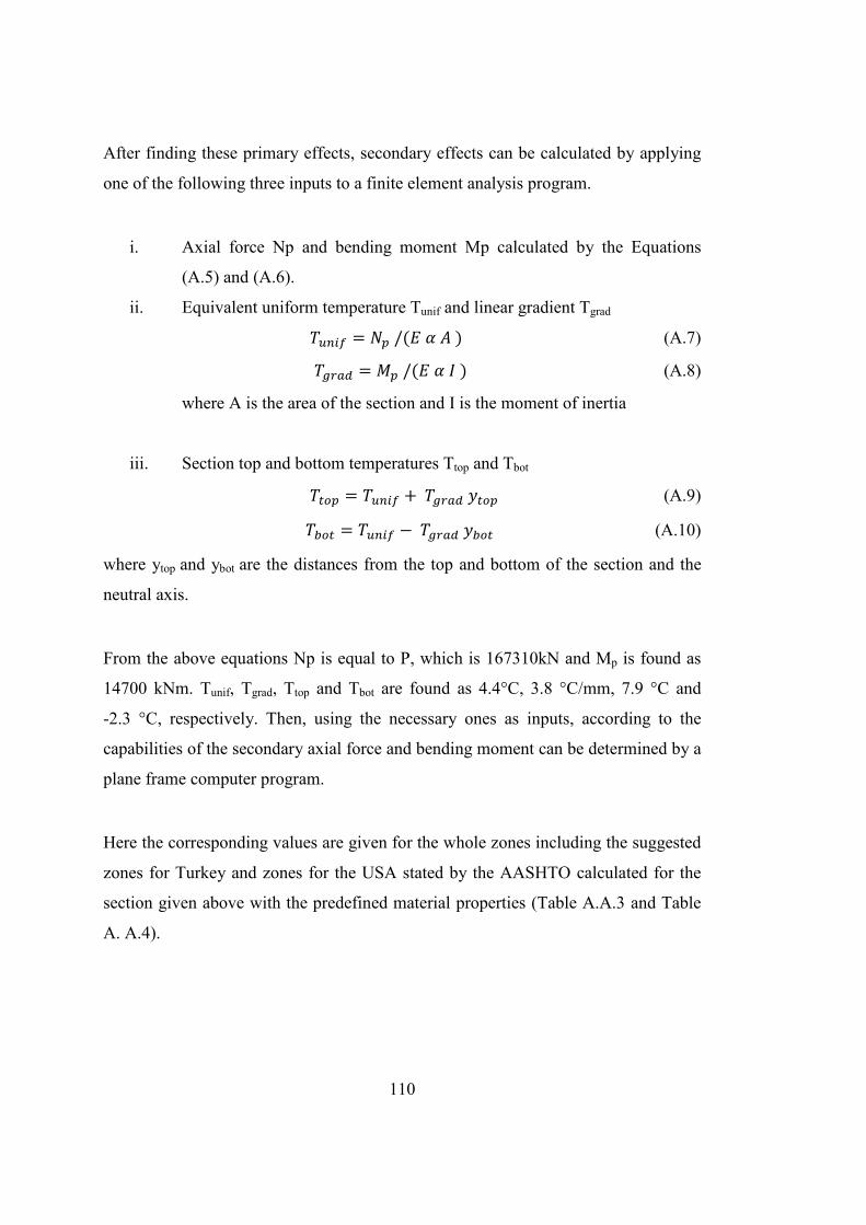
110
After finding these primary effects, secondary effects can be calculated by applying
one of the following three inputs to a finite element analysis program.
i. Axial force Np and bending moment Mp calculated by the Equations
(A.5) and (A.6).
ii. Equivalent uniform temperature Tunif and linear gradient Tgrad
𝑇𝑢𝑛𝑐𝑢 = 𝑁𝑝 /(𝐸 𝛼 𝐴 ) (A.7)
𝑇𝑎𝑔𝑎𝑔 = 𝑀𝑝 /(𝐸 𝛼 𝐼 ) (A.8)
where A is the area of the section and I is the moment of inertia
iii. Section top and bottom temperatures Ttop and Tbot
𝑇𝑡𝑖𝑝 = 𝑇𝑢𝑛𝑐𝑢 + 𝑇𝑎𝑔𝑎𝑔 𝑦𝑡𝑖𝑝 (A.9)
𝑇𝑏𝑖𝑡 = 𝑇𝑢𝑛𝑐𝑢 − 𝑇𝑎𝑔𝑎𝑔 𝑦𝑏𝑖𝑡 (A.10)
where ytop and ybot are the distances from the top and bottom of the section and the
neutral axis.
From the above equations Np is equal to P, which is 167310kN and Mp is found as
14700 kNm. Tunif, Tgrad, Ttop and Tbot are found as 4.4°C, 3.8 °C/mm, 7.9 °C and
-2.3 °C, respectively. Then, using the necessary ones as inputs, according to the
capabilities of the secondary axial force and bending moment can be determined by a
plane frame computer program.
Here the corresponding values are given for the whole zones including the suggested
zones for Turkey and zones for the USA stated by the AASHTO calculated for the
section given above with the predefined material properties (Table A.A.3 and Table
A. A.4).

111
Table A.A.3 Necessary Positive Temperature Gradient, Primary and Secondary Axial Load and Temperature Values to Calculate Secondary Thermal Effects
Zone Name T1 (°C)
T2 (°C) Pp (kN) Mp
(kNm) Tunif (°C)
Tgrad (m-1)
Ttop (°C)
Tbot (°C)
Turkey Recommended Zone 1 28 6 10264 8715 4.4 3.8 7.9 -2.3
Turkey Recommended Zone 2 25 6 9616 8137 4.1 3.5 7.4 -2.2
the USA Zone 1 30 8 11887 10032 5.1 4.4 9.1 -2.7 the USA Zone 2 25 7 10172 8580 4.4 3.7 7.8 -2.3 the USA Zone 3 23 6 9086 7664 3.9 3.3 7.0 -2.0 the USA Zone 4 21 5 8052 6812 3.4 3.0 6.2 -1.8
Table A. A.4 Necessary Negative Temperature Gradient, Primary and Secondary Axial Load and Temperature Values to Calculate Secondary Thermal Effects
Zone Name T1 (°C)
T2
(°C) Pp
(kN) Mp
(kNm) Tunif (°C)
Tgrad (m-1)
Ttop (°C)
Tbot (°C)
Turkey Recommended Zone 1 -6 -1 -2780 -2453 -1.3 -0.1 -1.4 -1.2
Turkey Recommended Zone 2 -5 -1 -2564 -2254 -1.2 -0.1 -1.3 -1.1
the USA Zone 1 -6 -2 -4171 -3638 -2.0 -0.2 -2.1 -1.9 the USA Zone 2 -5 -1 -2564 -2254 -1.2 -0.1 -1.3 -1.1 the USA Zone 3 -5 -1 -2564 -2254 -1.2 -0.1 -1.3 -1.1 the USA Zone 4 -4 -1 -2348 -2054 -1.1 -0.1 -1.2 -1.0
It is worthwhile to note that; the values calculated as Ttop and Tbottom are also get from
outputs of Larsa4D analysis and the same results are achieved.

112

113
APPENDIX B
B. THE TEMPERATURE AND SOLAR RADIATION DATA FOR THE ANALYZED CITIES
Figure B.1 Solar radiation data for Adana between Jan.2012-Dec.2012
Figure B.2 Temperature data for Adana between Jan.2012-Dec.2012

114
Figure B.3 Solar radiation data for Ankara between Jan.2012-Dec.2012
Figure B.4 Temperature data for Ankara between Jan.2012-Dec.2012

115
Figure B.5 Solar radiation data for Antalya between Jan.2012-Dec.2012
Figure B.6 Temperature data for Antalya between Jan.2012-Dec.2012
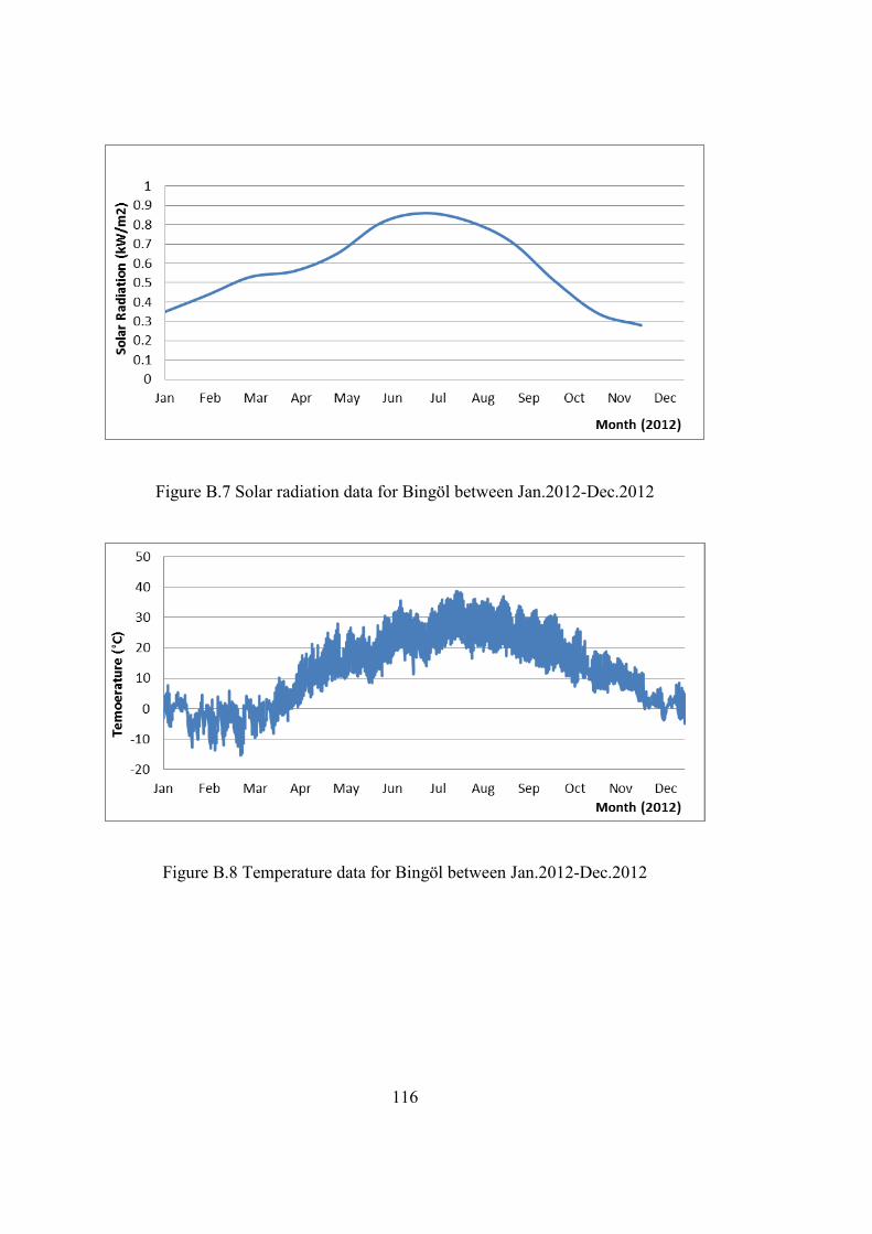
116
Figure B.7 Solar radiation data for Bingöl between Jan.2012-Dec.2012
Figure B.8 Temperature data for Bingöl between Jan.2012-Dec.2012
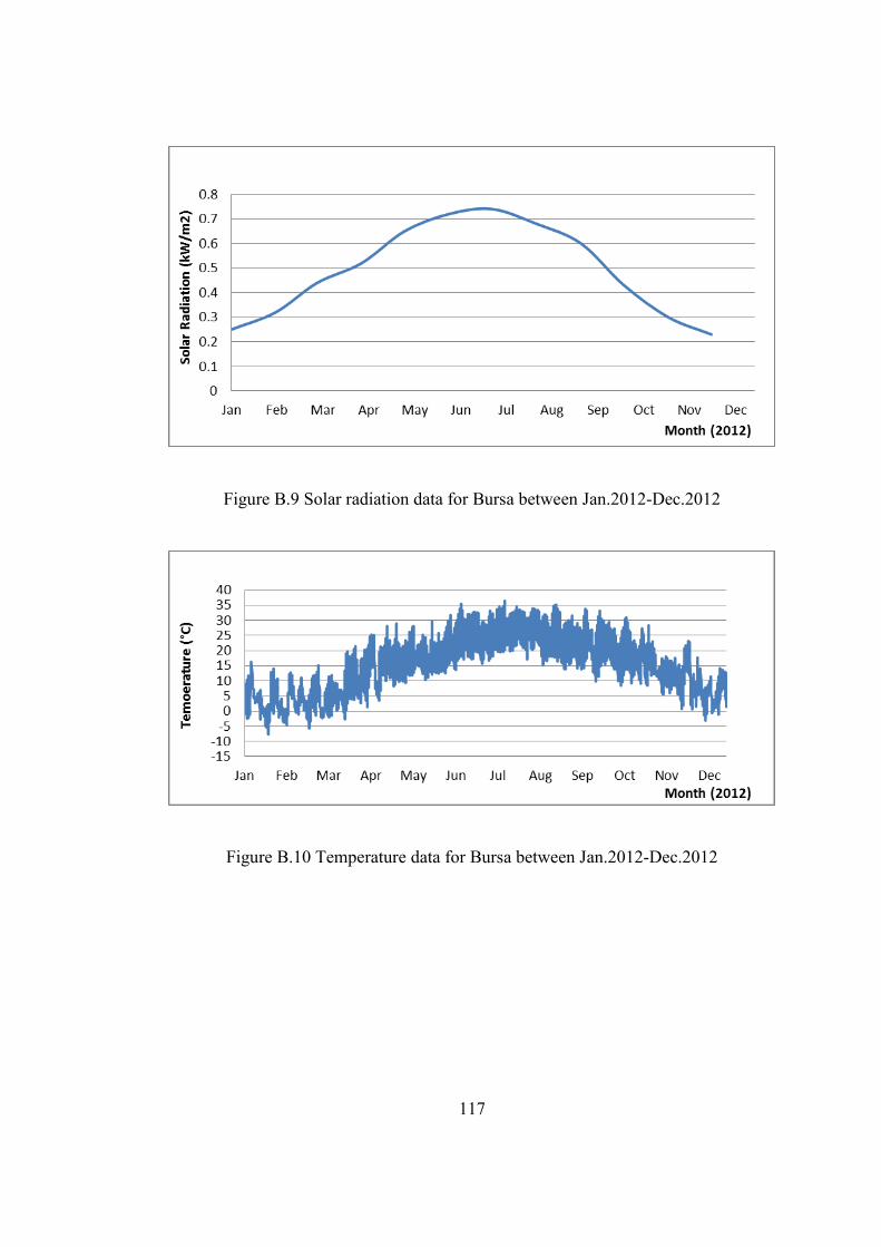
117
Figure B.9 Solar radiation data for Bursa between Jan.2012-Dec.2012
Figure B.10 Temperature data for Bursa between Jan.2012-Dec.2012

118
Figure B.11 Solar radiation data for Çanakkale between Jan.2012-Dec.2012
Figure B.12 Temperature data for Çanakkale between Jan.2012-Dec.2012

119
Figure B.13 Solar radiation data for Edirne between Jan.2012-Dec.2012
Figure B.14 Temperature data for Edirne between Jan.2012-Dec.2012
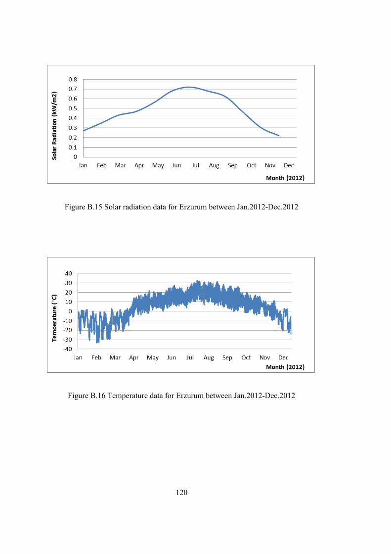
120
Figure B.15 Solar radiation data for Erzurum between Jan.2012-Dec.2012
Figure B.16 Temperature data for Erzurum between Jan.2012-Dec.2012
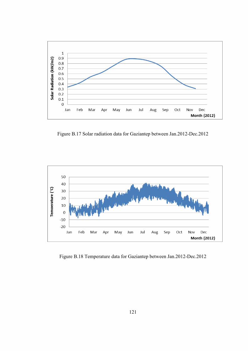
121
Figure B.17 Solar radiation data for Gaziantep between Jan.2012-Dec.2012
Figure B.18 Temperature data for Gaziantep between Jan.2012-Dec.2012
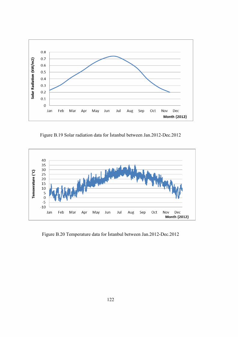
122
Figure B.19 Solar radiation data for İstanbul between Jan.2012-Dec.2012
Figure B.20 Temperature data for İstanbul between Jan.2012-Dec.2012
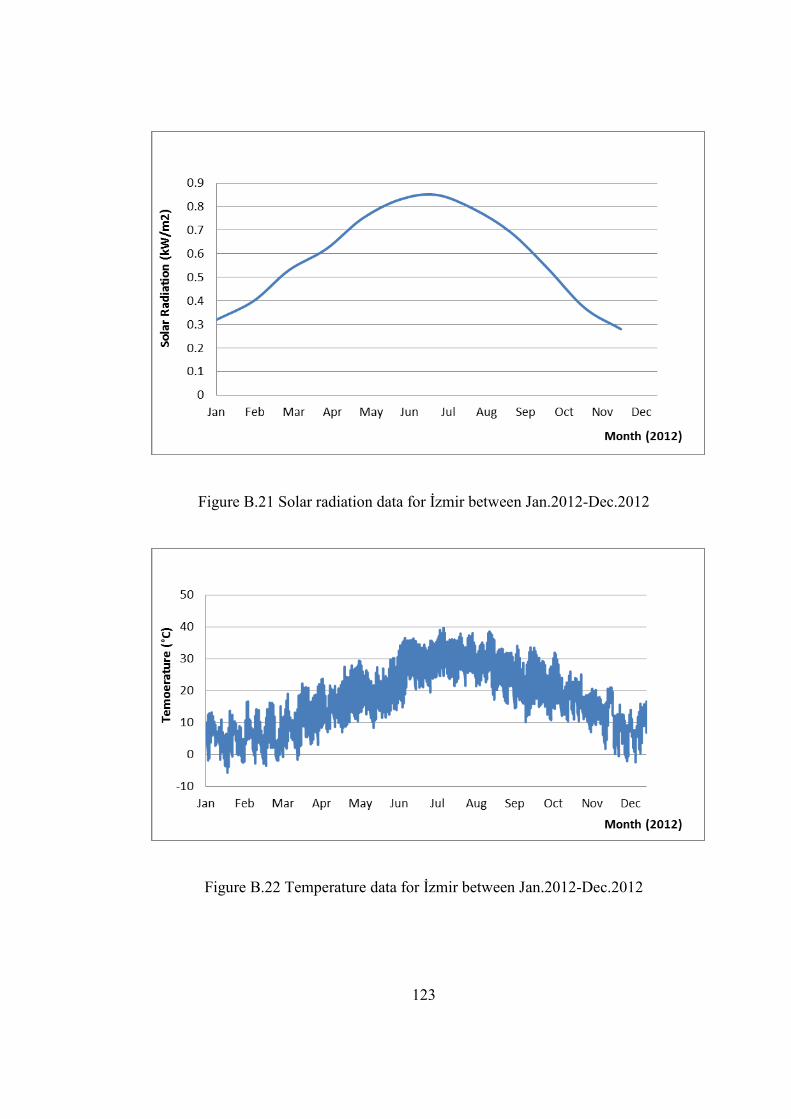
123
Figure B.21 Solar radiation data for İzmir between Jan.2012-Dec.2012
Figure B.22 Temperature data for İzmir between Jan.2012-Dec.2012
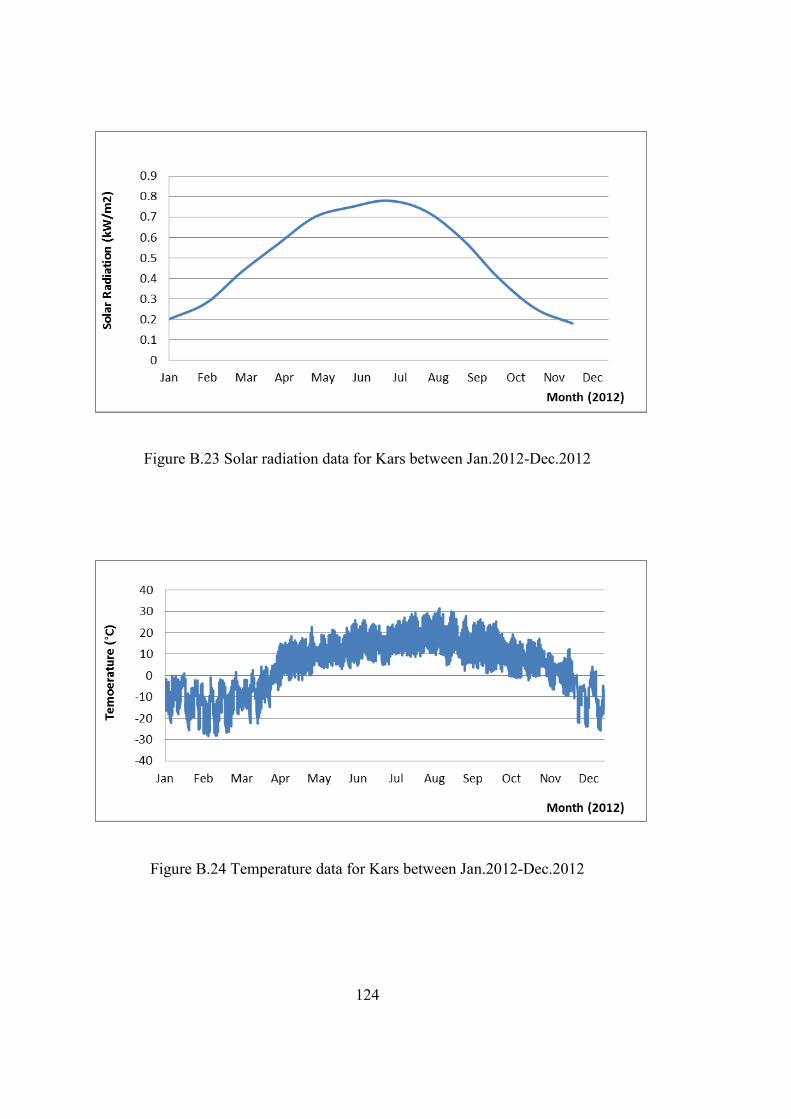
124
Figure B.23 Solar radiation data for Kars between Jan.2012-Dec.2012
Figure B.24 Temperature data for Kars between Jan.2012-Dec.2012

125
Figure B.25 Solar radiation data for Muğla between Jan.2012-Dec.2012
Figure B.26 Temperature data for Muğla between Jan.2012-Dec.2012
00.10.20.30.40.50.60.70.80.9
1
Jan Feb Mar Apr May Jun Jul Aug Sep Oct Nov Dec
Sola
r Rad
iatio
n (k
W/m
2)
Month (2012)
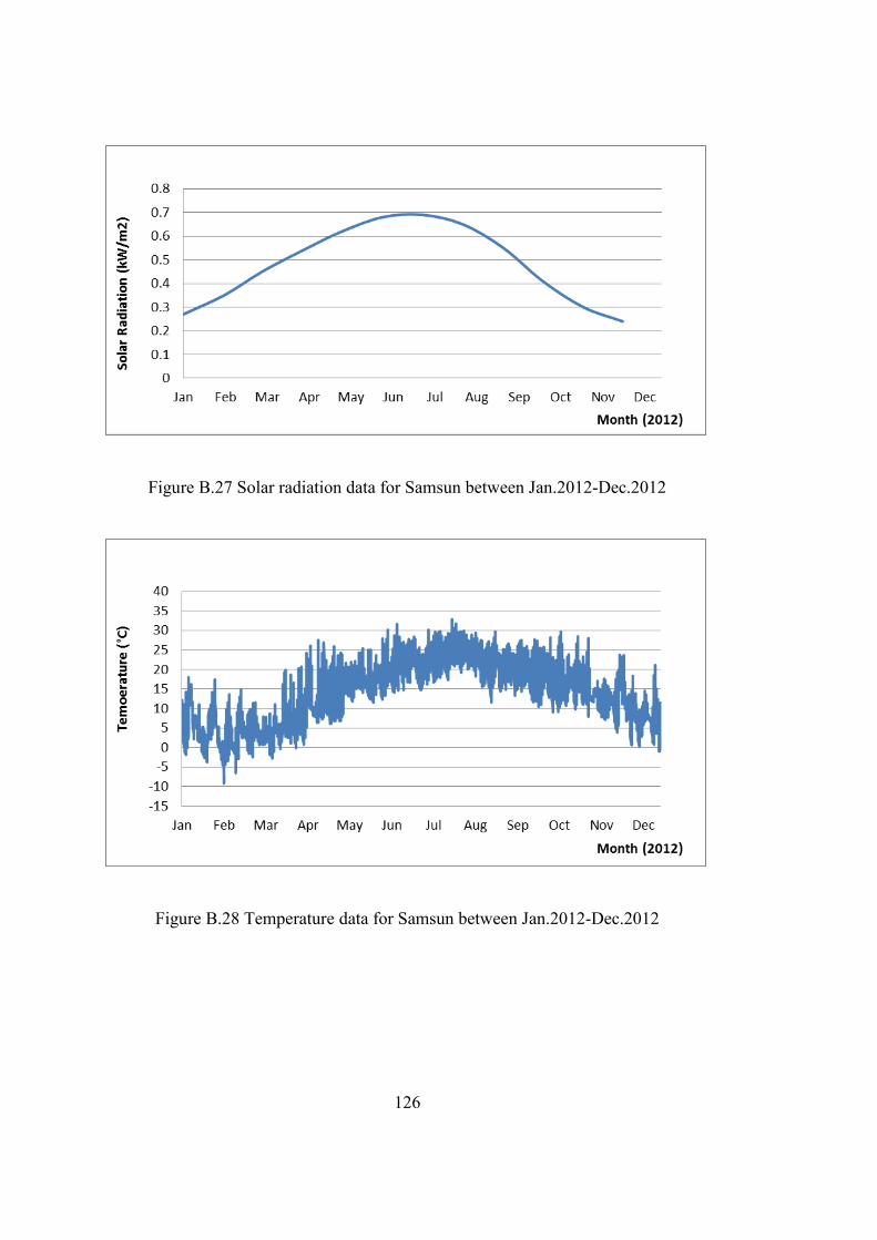
126
Figure B.27 Solar radiation data for Samsun between Jan.2012-Dec.2012
Figure B.28 Temperature data for Samsun between Jan.2012-Dec.2012
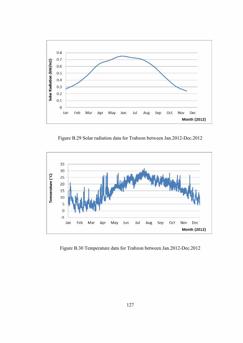
127
Figure B.29 Solar radiation data for Trabzon between Jan.2012-Dec.2012
Figure B.30 Temperature data for Trabzon between Jan.2012-Dec.2012
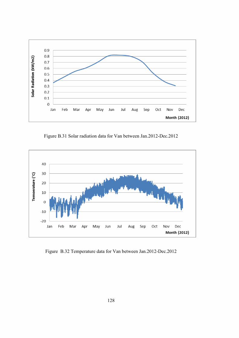
128
Figure B.31 Solar radiation data for Van between Jan.2012-Dec.2012
Figure B.32 Temperature data for Van between Jan.2012-Dec.2012