segmentation of abdominal organs from ct using a multi-level, hierarchical...
TRANSCRIPT

c o m p u t e r m e t h o d s a n d p r o g r a m s i n b i o m e d i c i n e 1 1 3 ( 2 0 1 4 ) 830–852
j o ur na l ho me pag e: www.int l .e lsev ierhea l th .com/ journa ls /cmpb
Segmentation of abdominal organs from CT usinga multi-level, hierarchical neural network strategy
M. Alper Selver ∗
Department of Electrical and Electronics Engineering, Dokuz Eylül University, Izmir 35160, Turkey
a r t i c l e i n f o
Article history:
Received 27 May 2013
Received in revised form
9 November 2013
Accepted 17 December 2013
Keywords:
Segmentation
Abdominal organ
CT
Hierarchical classification
a b s t r a c t
Precise measurements on abdominal organs are vital prior to the important clinical proce-
dures. Such measurements require accurate segmentation of these organs, which is a very
challenging task due to countless anatomical variations and technical difficulties. Although,
several features with various classifiers have been designed to overcome these challenges,
abdominal organ segmentation via classification is still an emerging field in order to reach
desired precision. Recent studies on multiple feature–classifier combinations show that hier-
archical systems outperform composite feature–single classifier models. In this study, how
hierarchical formations can translate to improved accuracy, when large size feature spaces
are involved, is explored for the problem of abdominal organ segmentation. As a result,
a semi-automatic, slice-by-slice segmentation method is developed using a novel multi-
level and hierarchical neural network (MHNN). MHNN is designed to collect complementary
information about organs at each level of the hierarchy via different feature–classifier com-
binations. Moreover, each level of MHNN receives residual data from the previous level.
The residual data is constructed to preserve zero false positive error until the last level of
the hierarchy, where only most challenging samples remain. The algorithm mimics analy-
sis behaviour of a radiologist by using the slice-by-slice iteration, which is supported with
adjacent slice similarity features. This enables adaptive determination of system parameters
and turns into the advantage of online training, which is done in parallel to the segmenta-
tion process. Proposed design can perform robust and accurate segmentation of abdominal
organs as validated by using diverse data sets with various challenges.
© 2013 Elsevier Ireland Ltd. All rights reserved.
segmentation is the most important step of the pipeline. How-
1. Introduction
Analysis (i.e. volume, size) and visualization of the abdom-inal organs (i.e. liver, spleen, right and left kidneys), tissues(i.e. lesions, tumors) and other structures in the abdomen (i.e.prostate [21], abdominal part of the aorta) are necessary and
important steps prior to several clinical procedures includingdiagnosis, therapy and surgery. Besides other modalities in usefor analysing abdominal region (such as MR [17] and PET [54]),∗ Tel.: +90 505 6487267.E-mail addresses: [email protected], [email protected]
0169-2607/$ – see front matter © 2013 Elsevier Ireland Ltd. All rights reshttp://dx.doi.org/10.1016/j.cmpb.2013.12.008
computed tomography-angiography (CTA) [27] is a widely usedradiographic technique. It has several advantages on bothclinical (i.e. allowing minimally invasive interventions) andtechnical (i.e. low radiation exposure, less acquisition time)sides [42]. For producing effective and clear visualizations ofabdominal organs and for obtaining precise measurements,
ever, two main issues, which are imposed by variations inhuman anatomy and image characteristics make the segmen-tation process extremely challenging.
erved.

c o m p u t e r m e t h o d s a n d p r o g r a m s i n b i o m e d i c i n e 1 1 3 ( 2 0 1 4 ) 830–852 831
Fig. 1 – Examples of abdominal CTA slices showing diversity and variations (a) very low contrast difference and unclearboundary between heart and liver; (b) unclear boundary due to partial volume effects between the right kidney and liver; (c)unclear boundary due to partial volume effects between left kidney and spleen; (d) contrast enhanced vascular tissuesinside liver parenchyma; (e) relatively less enhanced vessels compared to (d); and (f) multi-part liver, contrast enhancedk ey.
1
Uhwevbesvipsl
1
ItolipaHmd
a
idney tissues. Abbreviations: LK, left kidney; RK, right kidn
.1. Anatomical variations
nlike some relatively fixed organs in the body (i.e. brain), theuman anatomy in abdominal region shows great diversity,hich causes various changes in shape, size, orientation and
ven position of abdominal organs. This leads to countlessariations even in normal anatomy and prevents the use ofasic models. It is also not rare (e.g. 15% percent for liver Solert al. [48]) that patients have atypical organs (i.e. very unusualhape, texture, size, orientation or position). This diversity ofariations decreases the performance of several techniquesncluding [5], model (i.e. generalized cylinders as geometricrimitives [3], spatial [29], population-based geometric [50],tochastic [28] models) and atlas-based [56,41] analysis andimits their use to a subset of all cases.
.2. Technical difficulties
n CT imaging, rendering soft tissues have severe limita-ions due to their representation in a very narrow band ofverlapping Hounsfield (HU) value ranges [19]. This drawbackimits the performance of many techniques that are based onntensity (i.e. dynamical thresholding [31], gray level [55]), mor-hology [22] or their combination [2]). Moreover, the organsnd tissues can get very different values than their expectedU ranges in: (i) different patient data sets due to different
odality settings or (ii) different slices of the same data setue to injection of contrast media.Partial volume effects, patient movement, reconstruction
rtifacts and other external factors may cause blurred edges
and low contrast in the acquired images. Moreover, in CTA,the parenchyma of abdominal organs become inhomoge-neous due to the enhanced anatomical structures (i.e. vessels,tumors, lesions) (Fig. 1b–f), which become substructures thathave different textures. This prohibits the benefits of texturebased techniques [32], even when they are used in volumetricsense [35]. Thus, different processing techniques are requiredfor texture based approaches [14]. These inhomogeneities andblurring also limit emerging useful techniques that depend onthe homogeneity of gray levels and/or gradients in an image(i.e. level sets [43], region growing [52], fast marching [6], activecontours [26]).
There are also several studies that combine differentmethods to develop specific algorithms for abdominal organsegmentation [7,39,38,47,37]. These algorithms can be col-lected under the heading of rule-based techniques since theyincorporate some knowledge about anatomy and/or imagecharacteristics. Among those, especially for the liver, clini-cally promising results are reported in [23], which comparessuccessful algorithms using very detailed analysis. However,more research is still necessary until the abdominal organ seg-mentation problem can be considered largely solved, sinceeach limitation during segmentation can significantly reducethe correct measurement of quantitative parameters (i.e. vol-ume of an organ) [18].
Neural network (NN) based approaches are useful
alternatives in handling abdominal image segmentation.However, NN based segmentation procedures should bedesigned carefully in order to show enough and reliable per-formance. There are mainly two challenges that should be
s i n
832 c o m p u t e r m e t h o d s a n d p r o g r a mhandled properly in the field of abdominal image segmen-tation using NN. The first one is using preset parameters[2], which limits system performance due to wide ranges ofparameter values that differ significantly from data set to dataset. The second is the use of limited number of training datasets [1]. Naturally, supervised learning based NN models needa training set to train the NN. However, because of the diversevariations explained above, a huge number training sets arerequired to achieve acceptable performance.
For the use of NN based techniques for abdominal organsegmentation, several different features have been employed(i.e. spatial information [22], texture [14], intensity based [55]features). Each of these feature sets represents the abdominalorgans up to some level, but they all have their own drawbacks.For instance, intensity-based methods are successful in repre-senting homogeneous parenchyma, but have limitations dueto overlapping gray value ranges. On the other hand, texturesegmentation, which makes use of statistical textures anal-ysis to label regions based on their different textures, resultin a coarse and block-wise contour, leading to poor bound-ary accuracy. Boundary sensitive features can increase thisaccuracy, but they might skip inhomogeneities (due to con-trast media) in the parenchyma. As a result, it is obvious thata combination of features is needed to achieve a complete rep-resentation. Here, the critical point is the strategy of selectingthis combination, since no optimal way for it is found yet.
Therefore, an efficient strategy on combining features andclassifiers is required to overcome the challenges mentionedabove. Thus, in this study, the developed method is designedto:
• use multiple feature–classifier combinations in a multi-levelhierarchical scheme, where,– multi-level design provides each level to extract comple-
mentary information, which is typically from coarse (i.e.easier to classify) to detail (i.e. harder to classify),
– hierarchical design provides the use of residual data aftereach level (providing less data as levels proceed);
• adapt its parameters to the data and modify them accordingto the changes on it;
• use minimum user input (i.e. a single manually segmentedslice image for each organ) to perform supervised trainingin parallel to the segmentation process (i.e. not in advance).
The overall segmentation process developed in this studymainly depends on a 2-D classification task that is performediteratively for each slice of the data set. During the iterations,volumetric information is preserved by incorporating knowl-edge of previously segmented organs together with otherfeatures. For each slice image, classification is performed ina multi-level hierarchy in which, at each level, a differentfeature–classifier pair is employed to segment some part ofan organ. At the end, the results of all classifiers are combinedto obtain the segmentation result.
The rest of the paper is organized as follows: Section 2presents the related work and their comparisons with the pro-
posed approach. Section 3 introduces the data sets and organsof interest. Then, the novel multi-level, hierarchical radialbasis function network architecture is described in Section 4.Parameter determination methods for the proposed networkb i o m e d i c i n e 1 1 3 ( 2 0 1 4 ) 830–852
is discussed in Section 5. Section 6 presents applications andresults and finally, discussions and conclusions are given inSection 7.
2. Related work and motivation of thisstudy
As introduced in the previous section, accurate segmenta-tion of abdominal organs is a very difficult problem. Besidesthe availability of various known possibilities, the flexibilityof above listed parameters cannot be kept in strict bounds.Each new patient, thus each new data set, may have itsown and possibly unique challenges in addition to the com-mon problems. Therefore, the design and development ofa segmentation method for abdominal organs should bedone in a data-driven manner. As introduced in the pre-vious section, three important issues should be handledproperly.
2.1. Preset parameters
In abdominal organ segmentation problem, the ranges ofparameter values differ significantly from one data set toanother. These wide ranges decrease the efficiency of anymethod, when one utilizes a common parameter set (i.e. fixedthreshold value, predefined location) for all. Due to these highvariations in image characteristics, it is necessary to deter-mine the parameter values according to the data set that willbe segmented.
2.2. Training strategies
NN models that use supervised learning need training setsto adjust model weights. However, because of the diversevariations explained above, many training sets are needed toachieve acceptable performance. Unfortunately, it is not feasi-ble to construct a new training set and then train an NN eachtime a data set with different characteristics is introduced.As an alternative to these strategies, in which training isdone with a limited set of images [1], semi-automatic tech-niques that use some part of the data set to be segmentedas the training data, are proposed [2]. However, preparationof the training data by manually segmenting several slicesprior to the automated process is not practical from clinicalpoint of view. An alternative method is to use Hopfield NNwith unsupervised learning, where the segmentation proce-dure is formulated as a cost minimization problem [32]. Forimproving traditional design of Hopfield networks (i.e. archi-tectural limitations), contextual information is incorporatedin more advanced designs [9,36]. However, they could onlymake partial improvements over the traditional ones, sincethe results show that they fail at the regions where the graylevel of the desired region is too close to the adjacent tis-
sues.Due to these drawbacks of the training strategies, in thisstudy, the training procedure is performed in parallel to thesegmentation process.

i n b i
2
AtfHeotptTobfr
ibcf[wptiiaatb
3
3
TtCtD(oAtmmIists(ontdTt
c o m p u t e r m e t h o d s a n d p r o g r a m s
.3. Combining features
mong various features, one of the most important issues iso determine how to use them. In the simplest way, theseeatures can be lumped to construct a composite feature.owever, as shown in the literature [12,30] this has sev-ral disadvantages including computational complexity, cursef dimensionality, formation difficulty, increased processingime and redundancy. Moreover, the NN to process this com-osite feature essentially needs to be very complex andhis eventually results with reduced generalization capacity.herefore, in practice, a combination of features is needed tobtain a more complete representation. Since optimal com-ination and number of features is unknown, these diverseeatures are needed to be jointly used in order to achieveobust performance.
Therefore, a second approach, which is based on combin-ng multiple classifiers with diverse feature subset vectors, cane used. Of course, in this approach, the question of how toombine the classifiers has very drastic effects on system per-ormance. Among several methods that have been proposed24,8], no optimal strategy for combining multiple classifiers
ith diverse features is found yet. However, several studiesresent advantages of this second approach in many applica-ions including but not limited to speaker modeling [11] anddentification [13], handwriting recognition [53,49,25], qual-ty detection [45,44], volume visualization [46] hyper-spectralnalysis [33] and scene classification [16]. These successfulpplications, show that combining features and classifiers is aask that depends on the specific problem at hand, and shoulde handled with a data-driven strategy.
. Data sets and abdominal organs
.1. Liver transplantation donor database
he data sets used in this study were acquired after con-rast agent injection at portal phase using a Philips SecuraT with 2 detectors and a Philips Mx8000 CT with 16 detec-
ors, both equipped with the spiral CT option and located inokuz Eylül University Radiology Department. 20 data sets
CTA series), which were obtained by these scanners, consistf 12 bit DICOM images with a resolution of 512 × 512 per slice.ll of the 20 CTA series have 3–3.2 mm slice thickness and
his corresponds to a slice number around 90 (minimum 74,aximum 100 slices).Using spiral CT technique, respiratoryis-registrations between slices are reduced or eliminated.
ntra-slice pixel spacing of images are between 0.8 mm, whilenter-slice pixel spacing is between 3 and 3.2 mm. The dataets were retrospectively chosen to include different charac-eristics in terms of patient anatomy and acquisition. By doingo, the performance of the system in case of various challengesi.e. atypical anatomies, intensity changes due to the injectionf contrast media) can be tested. However, these data sets doot include any tumors and/or lesions for any organs, since
he aim of the study is to segment organs for transplantationonor candidates who are required to have healthy organs.he ground truth data is created based on manual segmenta-
ion using Philips IVM program, which is the current software
o m e d i c i n e 1 1 3 ( 2 0 1 4 ) 830–852 833
for evaluating volumes of transplantation donors in the clinic.The manual segmentation is performed by an expert radiolo-gist, who is experienced on pre-evaluation of transplantationdonors for more than 200 cases.
3.2. Sliver grand challenge database
Some of the image series employed in Sliver Grand Challenge[23] are also used in this study. These images were providedby several clinics, acquired from a variety of different CTscanners (i.e. 4, 16, and 64 detector rows) from different ven-dors. All of these data sets are also contrast enhanced in thevenous phase. Intra-slice pixel spacing of images are between0.55 and 0.8 mm, while inter-slice pixel spacing is from 1 to3 mm. Similar to donor database, the ground truth is generatedby radiological experts manually in transversal slice-by-slicefashion. The Sliver data sets are used for further evaluationof the MHNN algorithm in segmenting rotated images (i.e.protocols require patients to lie on their side thus the entireanatomy is rotated around an axis) and images with patholo-gies (i.e. tumors, metastasis and cysts of different sizes).
4. Multi-level, hierarchical neural networkstrategy
The developed multi-level, hierarchical NN (MHNN) designprovides a multi-step procedure for gathering all data thatbelong to an abdominal organ in a successive manner by asso-ciating different features and classifiers at each level of thehierarchy. Before describing the process, for the sake of clar-ity, level and hierarchy terms are defined and illustrated asfollows:
Level: A level is a sub-network, at which a single featureset-classifier combination is used to collect some part of thedesired information (i.e. partial information about an organ).This collected data should particularly correspond to the infor-mation which can be represented best by the feature set usedin that level (i.e. spatial features for location, texture featuresfor parenchyma, boundary features for organ borders)
Hierarchy: Basically, hierarchy is the successive use of thelevels. In MHNN, the levels are used in a cascaded manner,where the output of a level determines the input of the suc-ceeding one. The samples, which are classified at a level,are removed from the input sample space and the remaininginput samples are fed to the next level. Thus, each level (i.e.feature–classifier combination) is only responsible for the clas-sification of the data that can be correctly classified at thatlevel. And each feature space is used at a single level of clas-sification hierarchy. At the end, result of each level is mergedto construct the classification result.
Fig. 2 illustrates the general idea behind multi-level andhierarchy approaches, individually. Fig. 2a illustrates a featurespace (or the original data space) in which samples from fourdifferent classes are represented with different colors (i.e. red,
green, yellow, blue). The rectangular samples in each class rep-resent the samples, which are easier to classify in that featurespace. The circular samples are the ones that are harder toclassify and the triangular ones are the hardest.
834 c o m p u t e r m e t h o d s a n d p r o g r a m s i n b i o m e d i c i n e 1 1 3 ( 2 0 1 4 ) 830–852
Fig. 2 – Illustration of general idea behind Multi-level (a–c), hierarchical (d–f) classification scheme (4 classes: yellow, red,green, blue). (a) Feature space 1: the rectangular samples are the easiest ones to classify, the circular ones are harder and thetriangular ones are the hardest to classify; (b) feature space 2: the circular samples are the easiest ones to classify, thetriangular ones are harder and the rectangular ones are the hardest to classify; (c) feature space 3: the triangular samplesare the easiest ones to classify, the rectangular ones are harder and the circular ones are the hardest to classify; (d) simpleclassifiers to discriminate easiest samples to classify; (e) classified samples at (d) are removed and new simple classifiersare used; (f) process goes on until all samples are classified. (For interpretation of the references to color in this figure
e.)
legend, the reader is referred to the web version of the articlMulti-level approach: As shown in Fig. 2b, and c, in differ-ent feature spaces, the hardest samples to classify in Fig. 2amay become easier to classify. In Fig. 2b, the circular samplesare the easiest ones to classify, the triangular ones are harderand the rectangular ones are hardest to classify. On the otherhand, in Fig. 2c, the triangular samples are the easiest ones toclassify, the rectangular ones are harder and the circular onesare hardest to classify. Thus, the multi-level approach aims touse each feature space as a level, where, only the easiest sam-ples to discriminate at that space are classified. The remainingsamples are rejected for processing at the succeeding levels.
Hierarchical approach: In a feature space like Fig. 2a, it isvery hard to design a robust classifier that can correctly clas-sify the four classes at once. This is due to the circular andtriangular samples which are harder to classify. The attemptto classify these samples together with rectangular ones atthe same time often results with a complex classifier and lossof generalization capability. Instead, in hierarchical approach,
classification is done step by step with simpler classifiers. Asshown in Fig. 2d, first the easiest samples to classify are clas-sified and then these samples are separated from the data.Next, the harder ones are classified (Fig. 2e) and the processgoes on until the hardest samples are processed (Fig. 2f) (Notethat Fig. 2d–f both illustrate the same feature space).
In MHNN, the above mentioned multi-level and hier-archical approaches are used together. Each level, li(x),(feature–classifier combination) extracts its own representa-tion from the data, which results with measurements thatare unique to that level (Fig. 3). The idea behind this designis that different levels potentially offer complementary informa-tion, which should be combined to yield the best performance.Therefore, determination of the number levels and the typeof feature–classifier combinations, which will be used in thatlevel, are critical in the design of MHNN. These parametersdepend on the specific task at hand [34], in our case, abdominalorgan segmentation.
Proposed model of combining levels is especially importantand advantageous for the applications that require integrationof different types of features. The case of abdominal organsegmentation is such an application, in which the problem
consists of classes which can not be completely separatedwith a single feature–classifier combination because of partialoverlapping of features. The reason behind this advantageousbehaviour of MHNN is the fact that the efficiency is increased
c o m p u t e r m e t h o d s a n d p r o g r a m s i n b i
Fig. 3 – Multi-level, hierarchical classification strategy forsegmenting organ n
ictsaapicd
e
y
ti
noa
synaptic weight of the Gaussian unit at ith level.
n multilevel-classifier combinations due to use of simplerlassifiers and features in combination with a reject option. Inhe proposed MHNN strategy, this reject option carries unclas-ified samples (called rejected samples, which do not fall intony class at that level of hierarchy) to the next level of the hier-rchy, where another feature space and classifier combinationrocesses them. Since different features carry complimentary
nformation, the unclassified data at different levels do notompletely overlap and therefore, the amount of unclassifiedata is reduced as the levels proceed.
The MHNN system shown in Fig. 3 can be expressed math-matically as follows:
(x) =⋃N
n=1Cn(x) (1)
where⋃
is the set union operation that is used to mergehe segmented N organs (C1(x), C2(x), . . ., CN(x)) into the samemage y(x).
Each segmented organ, Cn(x), is constructed by a combi-
ation of the outputs of the all levels of hierarchy for thatrgan. Thus, complete segmentation output for an organ isfunction of the outputs of all levels, which can be denoted
o m e d i c i n e 1 1 3 ( 2 0 1 4 ) 830–852 835
by Cn(x) = Cn(C1n(x), C2
n(x), . . ., CKn (x)), where K is the number of
levels used to segment organ n.The ith level, li(x), has output Ci
n(x) which carries to thesamples that are classified in that level. On the other hand,the samples rejected at that level is denoted by uci
n(x).At each level, the rejected samples are calculated by remov-
ing classified data from the rest as ucin(x) = li(x) − Ci
n(x) and ingeneral
ucni + 1(x) = on(x) −i∑
j=1
Cjn(x) (2)
where on(x) is the original data.The critical point of the proposed strategy is not to include
any false-positive errors at level outputs. Instead, it is allowedand preferred to have false-negatives in rejected data. The rea-son behind is the fact that false-negatives can correctly beclassified at succeeding levels but false-positives can not becorrected as levels proceed, since they were directly includedin the result. Thus, one major challenge of the proposedsystem is to obtain a solution, which does not contain anyfalse-positive samples, among several possible solutions untilthe last level of the hierarchy. In other words, the hierarchicalsystem aims to make no false-positive mistakes until the lastlevel, where only the samples which are hardest to classifyremain. This approach has the advantage of making all falseclassifications at the end of the hierarchy, in expense of usingmultiple levels of classifications.
To be able to protect feasibility of the algorithm in terms ofcomputation and processing time, this multi-level classifica-tion scheme should be implemented with simple, yet effectiveclassifiers providing no false positive errors. For instance,usual perceptron learning is not adequate for this linearlynon-separable problem since error criterion is to minimize thetotal error of classification without favouring any classes (i.e.excluding false positives) (Fig. 4b). To achieve this goal withsimple classifiers, the pocket algorithm [20] is chosen. Thisalgorithm has the advantage of finding the optimum separa-tion plane among the possible solutions by means of positivecorrect ratio for linearly non-separable problems. Therefore,the procedure used to simulate the first n − 1 levels of the hier-archy is based on the pocket algorithm (Fig. 4a). As seen inseparating hyperplanes of Fig. 4b, pocket algorithm tries tominimize more false positive errors compared to perceptronlearning.
Finally, for the last level of hierarchy of each organ, Cin(x)
can be defined as,
Cin(x) = wi,j . gi,j(x − ci,j; �i,j) (3)
where gi,n(·) represents the Gaussian representingorgan n at the ith level and is defined by gi,n( · ) =exp((x − ci,n)T · (1/�2
i,n) · (x − ci,n)). Here, {ci,n|ci,n � RD}
represents center of the Gaussian unit, {�i,n|�i,n � RD} denoteswidth of the Gaussian unit, and {wi,n|wi,n � R} denoting the
If there exist more than one organ at a slice, whose assignedGaussian units overlap, then Gaussian widths are shrankaccording to the density of samples at overlapping region.

836 c o m p u t e r m e t h o d s a n d p r o g r a m s i n b i o m e d i c i n e 1 1 3 ( 2 0 1 4 ) 830–852
Fig. 4 – (a) The pseudo-code for the pocket algorithm. (b) First vs. second principal components of a statistical texturefeature space where blue samples belong to liver, red to right kidney, green to left kidney and black to spleen). Thedifference of separation planes to classify liver from others: Perceptron learning tends to provide best accuracy (orangecoloured separating plane), while pocket algorithm minimizes the false positive error (magenta coloured separating plane).
end
(For interpretation of the references to color in this figure legK-means clustering is used to determine the amount of theoverlapping by selecting number of clusters equal to the num-ber of overlapping organs. After clustering is performed, thewidth of a Gaussian unit is re-calculated using the distancefrom the Gaussian center to the sample at the border of thecorresponding cluster, as given below.
�i,n = min(ci,nxb), ∀i, n. (4)
Here �i,n is the width of the Gaussian unit at the ith level andxb is a sample at the border. Since the Gaussian units used inMHNN are not necessarily circular, the width search can finddifferent values for dimensions x1, x2, . . ., xr−1 in a r dimen-sional feature space. Gaussian units are used at the last levelof the MHNN system. The adjustment of the weights (i.e. train-ing of the RBFN), which is done similar to the other supervisedclassifiers that are used at the preceding levels of MHNN, isexplained in detail at the next section.
5. Segmentation using MHNN
To simplify the explanation of the developed segmentationmethod, the following terms are defined:
Slice: A slice refers to a single CTA image.Data set: A data set is the series of slices acquired for a patientduring a single CTA acquisition.
, the reader is referred to the web version of the article.)
Initial organ: An initial organ (i.e. initial liver, initial kidney,initial spleen) is the set of pixels of an organ in a 2D slice,which are manually segmented by the expert.Initial slice: Initial slice of an organ (i.e. initial liver slice, ini-tial kidney slice, initial spleen slice) is the slice number of thecorresponding initial organ.
Each abdominal organ of interest (i.e. liver, kidneys, spleen)is segmented individually using MHNN. During the process,possible overlappings are eliminated as described in Sec-tion 5.3.4.
5.1. Overview and initialization
The semi-automatic segmentation procedure of an abdominalorgan consists of two steps: (1) Selection of the initial sliceand manual segmentation of initial organ by an expert. (2) Thesegmentation of the organ at the remaining slices one by onestarting from the initial slice.
The segmentation algorithm starts from the initial sliceand first runs through the end of the data set. Then, start-
ing from the initial slice again, it runs through the beginningof the data set to complete the segmentation process. Thus,after the segmentation of the initial images, organs at otherslices are segmented iteratively.
c o m p u t e r m e t h o d s a n d p r o g r a m s i n b i o m e d i c i n e 1 1 3 ( 2 0 1 4 ) 830–852 837
edur
5c
AfitiTft
ttftdtb
istf
bttcppt
5
Tsc
Fig. 5 – (a) Initial training of a classifier; (b) training proc
.2. Initial and automatic training of the supervisedlassifiers
s discussed in the introduction, supervised training with anite training set in advance can introduce significant limita-ions over system performance due to the countless variationsn abdominal anatomy, acquisition and other parameters.herefore, an automatic online training method is designed
or MHNN, which perform training iteratively and in parallelo segmentation.
In the proposed automatic online training method, the ini-ial training is done using the initial slice (i.e. slice N − 1) andhe initial organ (Fig. 5a). For initial training of the network,eatures are extracted from the initial slice and used as theraining inputs of the network. The initial organ is used as theesired output and each input pixel is classified as belongingo the organ region or lying outside the organ region (on theasis of the training input).
After initial training is finished, weights are updated andteration proceeds to the next slice (i.e. slice N) (Fig. 5b). At thistep, the features are extracted for slice N i.e. the current sliceo segment). By using these features and the weights obtainedrom the previous slice (i.e. slice N − 1), slice N is segmented.
After the segmentation of slice N, network is trained againy using the features extracted from slice N as the input andhe new segmented image as the desired output. After theraining and calculation of the weights, the algorithm pro-eeds with the next slice (i.e. slice N + 1) and this iterativerocedure continues until all images are processed. Using thereviously adjusted weights as the initial weights of the nextraining phase, the training time is reduced significantly [47].
.3. Iterative and hierarchical segmentation
o realize the hierarchical classification described in previousection, features and classifiers should be combined in an effi-ient way (in terms of time and computational complexity). As
e of classifier N, which will be used to segment slice N.
shown in recent studies [33,11,16,45,46,44], this efficiency canbe provided by arranging the classification hierarchy in sucha way that:
(i) samples that can be classified with simpler featuresshould be classified at the earlier levels of the hierarchicalclassification process,
(ii) samples that are harder to classify should be classifiedby using more complex feature–classifier combinationsat the succeeding levels of the hierarchy,
(iii) features that provide complementary information shouldbe used at different levels in order to obtain improvedperformance.
This approach is very beneficiary in two ways: First, com-plex feature–classifier combinations are used to classify asless number of samples as possible, since the simpler onesare classified at the earlier stages of the hierarchy. This leadsto reduced computational time. Second, complex classifierscan perform higher success rates, since they only deal withclassifying the challenging samples.
Several feature sets can be employed independently at dif-ferent levels of the hierarchy during classification. The criticalpoint in the employment is to use complimentary informationprovided by different feature sets in a cascaded-hierarchicalmanner.
Each MHNN used in the segmentation of a slice consistsof a fixed number (i.e. four in this study) of levels. At eachlevel, classifier makes a binary decision whether a pixel repre-sents an organ or not. The outputs of the classifiers at eachof the four levels construct the overall classification result,when combined in an appropriate way. If a single level isused, all the features should be lumped together which cause
computational complexity, curse of dimensionality, formationdifficulty, increased processing time and redundancy.As shown in Fig. 3, process starts with the complete orig-inal data (i.e. image slice). At the first level, first feature set

838 c o m p u t e r m e t h o d s a n d p r o g r a m s i n b i o m e d i c i n e 1 1 3 ( 2 0 1 4 ) 830–852
Fig. 6 – (a) Original CT image and (b) distance transform of all organs together. Distance transform applied to: (c) the liver, (d)the right kidney and (e) the spleen.
is extracted and classification is performed. The pixels thatare labelled as organ are collected and the rest of the data issent to the next level. Then, using this rejected data as theinput, second feature set is extracted. After the classificationprocess, the pixels that belong to the organ are collected againand the rest of the data is sent to the next level. Afterwards,the unclassified samples (rejected data) are fed into the nextlevel and this process continues until all of the samples areclassified.
In this study, starting from the complete image data, first,a feature set that represents intensity and spatial informa-tion of the pixels is extracted. Since, the most basic elementsthat represent an organ is its position and intensity, thisfeature set is used at the first level of the hierarchy. Then,at the second level, 6 statistical textural features are cal-culated for the rejected data of the first level. Next, at thethird level 21 spectral textural features are extracted forthe rejected data of the second level. After classification atthe third level, only the most challenging samples (pixels),which belong mostly to boundary, are rejected. These dataare sent to the fourth level, where boundary information isextracted.
It can be noticed that, each succeeding level aims classify-ing pixels that are smaller in number but harder in difficulty.In other words, the first level aims to classify coarse areaand position of an organ. The second and the third levels
aim to classify parenchyma, where most of pixels belongingto an organ stands. Finally, the fourth level aims defin-ing organ boundary, which is usually the hardest and themost important part of the problem. Further details of theFig. 7 – The effect of level 1 on the features space. First vs. secona slice extracted from: (a) original image slice; (b) output of level
green to left kidney and black to spleen). (For interpretation of threferred to the web version of the article.)
classification process and levels are described at the followingsubsections.
5.3.1. Level 1: spatial information and intensityIn a very broad sense, the locations and intensities (i.e. HUvalues) of abdominal organs in a CTA image differ from eachother. Thus, these two properties can provide a coarse infor-mation for segmentation. Together with the computationalsimplicity of the extraction of these features, spatial infor-mation and intensity are well suited for the first level of theclassification hierarchy.
Since CT images are usually closely consecutive from thetop slice to the bottom slice, the location of the same organbetween adjacent slices are quite similar. Therefore, the regionof previously segmented organ at adjacent slice provides agood basis for searching the possible region of the organ ofinterest. In order to exploit the spatial location of an organ,the distance transform feature is used. The distance transformprovides a metric that measures the separation of the pix-els in an image. The metric is calculated to measure the totalEuclidean distance along the horizontal, vertical, and diago-nal directions. In MHNN algorithm, the distance transform isused to obtain information about the coarse location of anorgan at the adjacent (preceding/succeeding) slice (Fig. 6a andb). Since the size of an organ and its location does not change
dramatically between adjacent slices, the distance transformof a segmented organ gives a broad but totally correct infor-mation about the location of the same organ at the adjacentslice (Fig. 6b–e).d principal components of spectral texture feature space of1 (i.e. blue samples belong to liver, red to right kidney,e references to color in this figure legend, the reader is
c o m p u t e r m e t h o d s a n d p r o g r a m s i n b i o m e d i c i n e 1 1 3 ( 2 0 1 4 ) 830–852 839
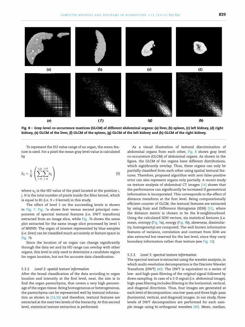
Fig. 8 – Gray-level co-occurrence matrices (GLCM) of different abdominal organs: (a) liver, (b) spleen, (c) left kidney, (d) rightk of t
tb
x
wji
ipepo(F
tof
5Alfiattel
idney, (e) GLCM of the liver, (f) GLCM of the spleen, (g) GLCM
To represent the HU value range of an organ, the mean fea-ure is used. For a pixel the mean gray level value is calculatedy
ij = 1N
⎛⎝
i+k∑i−k
j+k∑j−k
xij
⎞⎠ (5)
here xij is the HU value of the pixel located at the position i,. N is the total number of pixels inside the filter kernel, whichs equal to 81 (i.e. 9 × 9 kernel) in this study.
The effect of level 1 on the succeeding levels is shownn Fig. 7. Fig. 7a shows first versus second principal com-onents of spectral textural features (i.e. DWT transform)xtracted from an image slice, while Fig. 7b shows the samelot extracted for the same image slice processed by level 1f MHNN. The organ of interest represented by blue samples
i.e. liver) can be classified much accurately at feature space inig. 7b.
Since the location of an organ can change significantlyhrough the data set and its HU range can overlap with otherrgans, this level is only used to determine a candidate regionor organ location, but not for accurate data classification.
.3.2. Level 2: spatial texture informationfter the broad classification of the data according to organ
ocation and intensity at the first level, next, the aim is tond the organ parenchyma, that covers a very high percent-ge of the organ tissue. Being homogeneous or heterogeneous,
he parenchyma can be represented well by textural informa-ion as shown in [14,32] and therefore, textural features arextracted at the next two levels of the hierarchy. At this secondevel, statistical texture extraction is performed.he left kidney and (h) GLCM of the right kidney.
As a visual illustration of textural discrimination ofabdominal organs from each other, Fig. 8 shows gray levelco-occurrence (GLCM) of abdominal organs. As shown in thefigure, the GLCM of the organs have different distributions,which significantly overlap. Thus, these organs can only bepartially classified from each other using spatial textural fea-tures. Therefore, proposed algorithm with zero false-positiveerror can also represent organs only partially. A recent studyon texture analysis of abdominal CT images [14] shows thatthe performance can significantly be increased if geometricalinformation is incorporated. This corresponds to the effect ofdistance transform at the first level. Being computationallyefficient counter of GLCM, the textural features are extractedby using Sum and Difference Histograms (SDH) [51], wherethe distance metric is chosen to be the 8-neighbourhood.Using the calculated SDH vectors, six statistical features (i.e.mean, entropy (Fig. 9a), energy (Fig. 9b), skewness, dissimilar-ity, homogeneity) are computed. The well known informativefeatures of variance, correlation and contrast from SDH arealso extracted but reserved for the last level, since they carryboundary information rather than texture (see Fig. 10).
5.3.3. Level 3: spectral texture informationThe spectral texture is extracted using the wavelet analysis, inwhich multi-resolution decomposition is the Discrete WaveletTransform (DWT) [40]. The DWT is equivalent to a series oflow- and high-pass filtering of the original signal followed bydown sampling. In case of a 2-D signal (i.e. abdominal image),high-pass filtering includes filtering in the horizontal, vertical,and diagonal directions. Thus, four images are generated at
each level of decomposition: one low-pass and three high-pass(horizontal, vertical, and diagonal) images. In our study, threelevels of DWT decomposition are performed for each sam-ple image using bi-orthogonal wavelets [40]. Mean, median,
840 c o m p u t e r m e t h o d s a n d p r o g r a m s i n b i o m e d i c i n e 1 1 3 ( 2 0 1 4 ) 830–852
Fig. 9 – Sagittal analysis of an axial image series for volumetric analysis: (a) Pixels represented by entropy of sdh, (b) pixelsrepresented by energy of sdh, (c) pixels classified at the second level with spatial textures and (d) at the third level with
spectral textures.and variance of each level of decomposition are computed toobtain a feature vector for each sample.
Fig. 9 shows liver pixels collected by spatial and spectralfeatures on a sagittal image to illustrate their coverage in a vol-umetric sense. Fig. 9a and b shows entropy and energy featuresextracted from SDH, respectively, both of which can representparenchyma partially. Fig. 9c shows classified pixels at the sec-ond level, while Fig. 9d shows complementary textural dataclassified at the third level. The non-overlapping complemen-tary information represented by spatial and spectral texturefeatures is clearly visible.
5.3.4. Level 4: boundary informationIn abdominal CT images, distinct boundaries may not existbetween the neighbouring organs to enable edge detectionof organ boundaries. Furthermore, the boundaries may be
Fig. 10 – Application of boundary extractors to output of third levvariance of SDH, (d) Canny detector, (e) Laplacian detector and (f)
blurred and became ambiguous due to partial volume effects.These problems make the segmentation of the boundaries ofthe neighbouring organs a challenging task and therefore, thepixels belonging to the boundaries are usually the hardestsamples to classify. Hence, the boundary information is han-dled as the fourth and the last level of the hierarchy, wherethe samples belonging to the parenchyma are classified at thefirst three levels of the system. To perform boundary extrac-tion, two kinds of features are combined: (i) textural boundaryextractors, (ii) edge detectors. As mentioned in level 2, fea-tures of correlation (Fig. 10a), contrast (Fig. 10b) and variance(Fig. 10c) from SDH are used as boundary extraction fea-
tures. The advantage of these features is that they representboundaries as a set of connected components. But dependingon the feature used, they also represent outer and/or adja-cent boundaries as connected components. Although, thisel of MHNN: (a) correlation of SDH, (b) contrast of SDH, (c) correlation of SDH multiplied by Laplacian.

i n b i
dr
eatnneop
af4csrswafw
eFfc
5Fcctttwo
C
tdcewspsml
flisft
c o m p u t e r m e t h o d s a n d p r o g r a m s
rawback is reduced at level 1, the clarity of informationequires improvement on boundary representation.
The second extractor set, edge detection algorithms,ither simple (i.e. high pass filters) or complicated (i.e.nisotropic diffusion) use sharpening at some level to enhancehe boundary information, which deforms the homoge-eous parenchyma information. This can cause extraction ofon-boundary regions as boundary. This trade-off betweenxtracting boundary information in detail and preservingrgan parenchyma is resolved by classification of thearenchyma at the preceding levels of MHNN.
Moreover, boundary extraction should be performed with kernel that is sensitive to the effects of the distance trans-orm. For instance, considering an exemplary input of level
(Fig. 13), two well known edge detectors, Canny and Lapla-ian are compared. As shown in Fig. 10d and e, Canny is notensitive to distance transform effect, while Laplacian resulteflects adjacent boundary similarity in a much better way. Aimilar approach is used in [15] for hierarchical shape models,hich shows not only performance increase due to less vari-
tions exhibited by residual parts (compared to the variationsor the complete shape), but also these parts can be capturedith fewer training samples.
By combining edge detectors with textural boundaryxtractors, more informative descriptors can be obtainedig. 10f. In MHNN, such boundary features are used as theeatures of the last level, where RBFN networks perform finallassification task.
.3.5. Combining MHNN outputs and post-processingor combining outputs of the levels, a decision making pro-edure is used instead of simply merging the outputs of alllassifiers. The decision procedure relies on a predefined cri-erion, but it may also be determined according to data duringhe process. After all levels of the classification is completed,he results of each level are combined using the rule below,here ∩ indicates set intersection, and ∪ indicates set unionperations.
n(x) = (on(x) ∩ C1n(x)) ∩ (
⋃4
k=2Ck
n(x)) (6)
Since the first level result carries broad location informa-ion for the organ of interest, its intersection with the originalata remains organ’s coarse topology information. At the suc-eeding levels, parenchyma and boundary information arextracted and united. The intersection of these levels (i.e. 2–4)ith the coarse topology of corresponding organ results with
egmented organ data. Depending on the organ, some minorost-processing operations (i.e. hole filling, slight boundarymoothing) are applied to fine tune and obtain a concrete seg-ented region. Fig. 13 shows examples of the results of each
evel and their combination for liver.After combining the classification results of different levels
or an organ, a series of morphological operations and non-inear filtering techniques are used to refine the output. These
nclude removal of mis-segmented small objects, boundarymoothing, and multiple component identification (i.e. mostlyor liver). During this process, first, a median filter is appliedo remove the white spots appear at the background (falseo m e d i c i n e 1 1 3 ( 2 0 1 4 ) 830–852 841
positives) and black spots appear inside the organs (false neg-atives). Then, erosion operation is applied to eliminate thesmall unconnected objects that do not sit within the structur-ing element. Next, the skeleton of the previously segmentedliver is obtained using skeletonisation. Finally, by using binarymorphological image reconstruction, in which the skeletonis used as the marker image and MHNN output as the maskimage, the organ is identified. This post-processing strategy isdescribed in detail at [47].
6. Applications and results
In order to reflect the performance of the proposed system,two evaluation methods are performed. First, the classificationstrategy is evaluated (see Section 6.1) and then, the segmenta-tion algorithm performance is tested (see Section 6.2).
6.1. Evaluation of the classification strategy
The proposed MHNN strategy is compared to two techniques.The first one is the composite feature–single classifier (CFSC)approach and the second one is the Ascendant HierarchicalClustering (AHC) technique proposed by [4]. AHC decomposesa K-class classification problem into K − 1 binary classificationproblems by using distance measures to investigate the classgrouping in binary form at each level in the hierarchy. Themethod consists of two steps: first, AHC is applied over theclass centers, which can be determined by using the train-ing data, to obtain the hierarchical tree. In the second step,an SVM classifier is employed at each node of the tree andis trained with the elements of the two subsets of the node.AHC is adopted to the proposed segmentation scheme by cal-culating the centers of the four classes (organs) using thepreviously segmented image (i.e. training data). By this wayproposed multi-level hierarchy is compared to ascendant hier-archy using the same segmentation method.
The comparative simulations are performed in two ways.First, MHNN, CFSC and AHC algorithms are trained using theground-truth data. In other words, slice K is segmented usingthe distance transform and training features extracted fromground truth of slice K − 1. This corresponds to best possiblecase, since an organ in slice K is segmented using the best pos-sible previous segmentation result, which is the ground truthof that organ at slice K − 1 (i.e. initial organ). When appliedto all image slices in our data set, the classification resultsprovide the upper-bound of accuracy for the algorithms. Theseresults (Fig. 11) show that MHNN outperforms both CFSC andAHC approaches in terms of accuracy (CC), false negative rate(FN), false positive rate (FP), Selectivity (SE) and Specificity (SP).Moreover, the results also show that MHNN algorithm canperform up to 2.93%, 2.32%, 3.83%, 4.23% FP + FN percentagesfor RK, LK, S and L respectively. Although AHC’s performanceis very close to MHNN for the right and left kidneys, theirperformance differs for spleen and liver. This is a very high
performance compared to the results presented in the lit-erature and shows that the upper bound of MHNN systemperformance is good enough to discuss its use in actual itera-tive segmentation.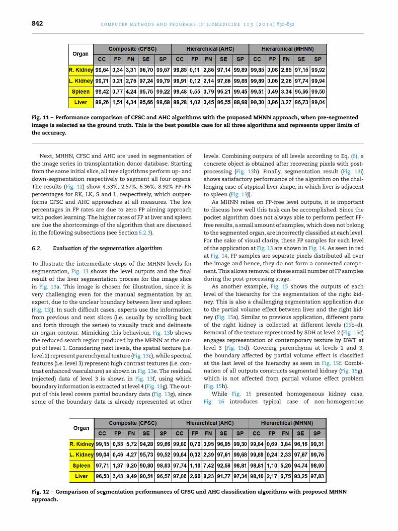
842 c o m p u t e r m e t h o d s a n d p r o g r a m s i n b i o m e d i c i n e 1 1 3 ( 2 0 1 4 ) 830–852
Fig. 11 – Performance comparison of CFSC and AHC algorithms with the proposed MHNN approach, when pre-segmentedimage is selected as the ground truth. This is the best possible case for all three algorithms and represents upper limits of
the accuracy.Next, MHHN, CFSC and AHC are used in segmentation ofthe image series in transplantation donor database. Startingfrom the same initial slice, all tree algorithms perform up- anddown-segmentation respectively to segment all four organs.The results (Fig. 12) show 4.53%, 2.57%, 6.36%, 8.92% FP+FNpercentages for RK, LK, S and L, respectively, which outper-forms CFSC and AHC approaches at all measures. The lowpercentages in FP rates are due to zero FP aiming approachwith pocket learning. The higher rates of FP at liver and spleenare due the shortcomings of the algorithm that are discussedin the following subsections (see Section 6.2.3).
6.2. Evaluation of the segmentation algorithm
To illustrate the intermediate steps of the MHNN levels forsegmentation, Fig. 13 shows the level outputs and the finalresult of the liver segmentation process for the image slicein Fig. 13a. This image is chosen for illustration, since it isvery challenging even for the manual segmentation by anexpert, due to the unclear boundary between liver and spleen(Fig. 13j). In such difficult cases, experts use the informationfrom previous and next slices (i.e. usually by scrolling backand forth through the series) to visually track and delineatean organ contour. Mimicking this behaviour, Fig. 13b showsthe reduced search region produced by the MHNN at the out-put of level 1. Considering next levels, the spatial texture (i.e.level 2) represent parenchymal texture (Fig. 13c), while spectralfeatures (i.e. level 3) represent high contrast textures (i.e. con-trast enhanced vasculature) as shown in Fig. 13e. The residual
(rejected) data of level 3 is shown in Fig. 13f, using whichboundary information is extracted at level 4 (Fig. 13g). The out-put of this level covers partial boundary data (Fig. 13g), sincesome of the boundary data is already represented at otherFig. 12 – Comparison of segmentation performances of CFSC andapproach.
levels. Combining outputs of all levels according to Eq. (6), aconcrete object is obtained after recovering pixels with post-processing (Fig. 13h). Finally, segmentation result (Fig. 13i)shows satisfactory performance of the algorithm on the chal-lenging case of atypical liver shape, in which liver is adjacentto spleen (Fig. 13j).
As MHNN relies on FP-free level outputs, it is importantto discuss how well this task can be accomplished. Since thepocket algorithm does not always able to perform perfect FP-free results, a small amount of samples, which does not belongto the segmented organ, are incorrectly classified at each level.For the sake of visual clarity, these FP samples for each levelof the application at Fig. 13 are shown in Fig. 14. As seen in redat Fig. 14, FP samples are separate pixels distributed all overthe image and hence, they do not form a connected compo-nent. This allows removal of these small number of FP samplesduring the post-processing stage.
As another example, Fig. 15 shows the outputs of eachlevel of the hierarchy for the segmentation of the right kid-ney. This is also a challenging segmentation application dueto the partial volume effect between liver and the right kid-ney (Fig. 15a). Similar to previous application, different partsof the right kidney is collected at different levels (15b–d).Removal of the texture represented by SDH at level 2 (Fig. 15c)engages representation of contemporary texture by DWT atlevel 3 (Fig. 15d). Covering parenchyma at levels 2 and 3,the boundary affected by partial volume effect is classifiedat the last level of the hierarchy as seen in Fig. 15f. Combi-nation of all outputs constructs segmented kidney (Fig. 15g),
which is not affected from partial volume effect problem(Fig. 15h).While Fig. 15 presented homogeneous kidney case,Fig. 16 introduces typical case of non-homogeneous
AHC classification algorithms with proposed MHNN

c o m p u t e r m e t h o d s a n d p r o g r a m s i n b i o m e d i c i n e 1 1 3 ( 2 0 1 4 ) 830–852 843
Fig. 13 – Segmentation of liver with MHNN strategy: (a) original image slice, (b) output of the first level after application ofdistance transform and mean features, which is also the input of the second level, (c) output of the second level (i.e.statistical texture), (d) residual data and input of the third level, (e) output of the third level (i.e. spectral texture), (f) residualdata and input of the fourth level, (g) output of the fourth level (i.e. boundary), (h) pixels recovered by post-processing, (i)segmentation result and (j) challenging liver–spleen boundary
k2ttmcw
icibaiwal
Foa
idney parenchyma. As shown in Fig. 16, outputs of level (Fig. 16b) and level 3 (Fig. 16c) represent complementaryextural information resulting complete segmentation whenhey are unified (Fig. 16e) according to (6). Similar to liver seg-
entation in Fig. 14, this example shows the robustness of thelassification strategy to heterogeneous organ parenchyma,hich usually occur at contrast enhanced studies.
A challenging case of spleen segmentation is presentedn Fig. 17. Homogeneous texture of spleen allows satisfactorylassification without using all levels of the hierarchy in major-ty of the cases. However, there exist two partial volume effectased challenges in this image; one with the left kidney (yellowrrow in Fig. 17b) and another with a similar tissue (red arrown Fig. 17b). The application of MHNN discriminates boundary
ith the left kidney at the second level of the hierarchy (yellowrrow in Fig. 17b), while the latter challenge is resolved at theast level of the hierarchy (red arrow in Fig. 17d). Thus, instead
ig. 14 – Samples classified as FP (a) at the output of the second
f the fourth level. (For interpretation of the references to color inrticle.)
of dealing with all challenging tasks at once, MHNN strategyhandles difficulties at its different levels effectively as shownin this application.
The applications introduced so far present the strongpoints of the MHNN. Following sections discuss further evalu-ation of the algorithm with additional metrics (Section 6.2.1),application of MHNN to Sliver data sets [23] (Section 6.2.2),shortcomings of the algorithm (Section 6.2.3), and its compu-tational performance (Section 6.2.4).
6.2.1. Evaluation on transplantation donor databaseIn this part of the evaluation, segmentation performance ismeasured using area error rate (AER) metric, which is shown
to be effective in the evaluation of liver from transplantationdonor data sets [47]. AER is defined as the area differencebetween the region segmented by the algorithm (RA) and theregion segmented manually (RM). Defining a Union Region (RU)level, (b) at the output of the third level and (c) at the output the text, the reader is referred to the web version of the

844 c o m p u t e r m e t h o d s a n d p r o g r a m s i n b i o m e d i c i n e 1 1 3 ( 2 0 1 4 ) 830–852
Fig. 15 – Segmentation of the right kidney with MHNN strategy: (a) output of the first level after application of distancetransform and mean features, (b) output of the second level (i.e. statistical texture), (c) residual data and input of the thirdlevel, (d) output of the third level (i.e. spectral texture), (e) residual data and input of the fourth level, (f) output of the fourthlevel (i.e. boundary information), (g) segmented kidney after combining of the outputs of all levels and post-processing, (g)segmented kidney and (h) contour of segmented kidney area drawn on the original image.
Fig. 16 – Segmentation of the right kidney with MHNN strategy: (a) distance transform of the original image, (b) output ofthe second level (i.e. statistical texture), (c) output of the third level (i.e. spectral texture), (d) output of the last level (i.e.boundary) and (e) segmented kidney with a small mis-segmented part (see Section 6.2.3).
Fig. 17 – Segmentation of spleen with MHNN strategy: (a) distance transform of the original image, (b) output of the secondlevel (partial volume effect with kidney is resolved by including overlapping part in segmentation result), (c) residual data,(d) rejected data at the third level (partial volume effect with unknown tissue is resolved by excluding the tissue fromsegmentation result) and (e) rejected overlapping tissue. (For interpretation of the references to color in the text, the readeris referred to the web version of the article.)

c o m p u t e r m e t h o d s a n d p r o g r a m s i n b i o m e d i c i n e 1 1 3 ( 2 0 1 4 ) 830–852 845
irect
ae
A
pebeidetea
(
(
scwtao
pukmAAT
Fig. 18 – Area error rate results of d
s RA ∪ RM and an Intersection Region (RI) as RA ∩ RM, AER isqual to:
ER(%) = RU − RI
RM× 100 (7)
Direct comparison of segmented and reference dataroduces an evaluation, which is very sensitive to differ-nces in between. For instance, even a single pixel differenceetween segmented and reference data may increase therror rate significantly although, no modification is neededn practice. As very well known, the reference data itself isependent to the expert and might vary slightly from onexpert to another. Therefore, the evaluation strategy shouldolerate these slight differences between segmented and ref-rence data. Considering the above mentioned issues, resultsre evaluated with two approaches:
1) Direct quantitative evaluation (DQE): AER is used directlyto evaluate the differences between segmented and refer-ence data.
2) Qualitative followed by quantitative evaluation (QQE): seg-mented images are first reviewed by the expert. Then, onlythe slices that need modification are evaluated with AER.
In general, the results show that the organs of interest areegmented with satisfactory performance, but we can con-lude that the right kidney and left kidney are segmentedith high performance. This is mainly because of their rela-
ively simpler shape and smaller size. On the other hand, livernd spleen has more AER due to their complex size shape andrientation.
Fig. 18 shows average DQE AER for each organ at eachatient data set. DQE evaluation presents average AER val-es of 8.14% for liver, 8.02% for spleen, 6.26% for the rightidney, and 5.97% for the left kidney. Being the biggest and
ost complicated among others, the liver has the highestER as expected. The difference between right and left kidneyER values is due to the difference of their adjacent organs.he right kidney is significantly close to liver and boundaryquantitative evaluation (DQE AER).
between them is very unclear especially at the slices, wherethe right kidney begins to appear. Although, spleen has a sim-ilar texture with liver, it is more compact in shape, smallerin size and its boundary is usually distant from the left kid-ney. Thus, the left kidney can be segmented more accuratelycompared to the right kidney.
The slice by slice average AER for 20 data sets for liveris shown in Fig. 19, which also presents a comparison with[47]. In [47], it was observed that AER values are higher dueto the unclear boundaries between hearth–liver (i.e. slices atthe beginning) and between the right kidney–liver (i.e. slicesat the end). The average DQE AER for all data set was calcu-lated as 12.15%. In this study, the performance is improvedsignificantly both in average (AER = 8.13%) and in the slices atthe beginning/end of the data sets. This improvement is dueto better segmentation of liver–kidney and heart–liver bound-aries by using the proposed method.
A comparison to the results of [23], where semi-automaticmethod finalists (i.e. the top 7 out of 9 contestants) had Vol-umetric Overlap Error (VOE) below 8.1%, is also performed.VOE is a similar metric to AER except the denominator is themanual segmentation in AER, while it is the union (i.e. theJaccard distance) in VOE. Moreover, AER provides a wider eval-uation range since VOE is limited between range 0 and 100 (0for perfect segmentation and 100, when there is no overlapat all between segmented and reference data). AER is also 0for perfect segmentation, however the worst case value is notlimited to 100. Therefore, VOE evaluation of liver results inthis study have an average value of 7.97%. This is a slightlybetter performance than Sliver context results in average [23].However, a direct comparison is not possible since Sliver con-text data include tumors, while the algorithm in this study isdesigned to segment healthy organs such as transplantationcandidates. Therefore, a more detailed comparison with Slivercontext is reported in the following subsection.
The slice by slice average AER for 20 data sets for spleen,
the right and left kidneys are shown in Fig. 20. Besides clin-ically acceptable performance of the algorithm, this figureshows a uniform AER distribution among slices, which refersthat these organs are segmented without mistakes even when
846 c o m p u t e r m e t h o d s a n d p r o g r a m s i n b i o m e d i c i n e 1 1 3 ( 2 0 1 4 ) 830–852
Fig. 19 – Average AER calculated for the slices, which have identical number, in all data sets for liver (i.e. the errorpercentage for the 40th slice represents the average AER of 40th slices in all data sets). Red lines show the results of thisstudy, while the blue ones show the results obtained at [47]. The increased performance of the MHNN is significant in theslices at the end, where liver and the right kidney commonly mis-segmented in [47]. (For interpretation of the references to
ersi
color in this figure legend, the reader is referred to the web vtheir adjacent organs appear/disappear among slices. This isan important advantage of the proposed design since manyalgorithms show reduced segmentation performance in theexistence of adjacent organs, especially at the slices whenthese adjacent organs begin to appear and/or disappear.
As mentioned above, AER is very sensitive to the pixeldifferences between automatically and manually segmentedimages. Although, a small number of pixel differencesbetween RA and RM regions are practically not important, they
Fig. 20 – Average AER calculated for the slices, which have identispleen.
on of the article.)
increase the AER significantly. Therefore, QQE is used, in whichexpert radiologist choose the slices that need further modifica-tion. Then, AER is calculated only for those slices. Fig. 21 showsthe average AER calculated for the slices that need modifica-tion for each patient data set by using the overall system. The
results show that the average AER is reduced significantly to7.17% in average with a minimum of 6.03% and a maximumof 9.91% for liver, 6.11% in average with a minimum of 5.15%and a maximum of 8.32% for spleen, 3.98% in average withcal number, in all data sets for left kidney, right kidney and

c o m p u t e r m e t h o d s a n d p r o g r a m s i n b i o m e d i c i n e 1 1 3 ( 2 0 1 4 ) 830–852 847
foll
akm
pmsivsApiit3ac
6Tstctmalaa3i5e
ffaa
Fig. 21 – Area error rate results of qualitative
minimum of 1.68% and a maximum of 5.07% for the rightidney and, 3.56% in average with a minimum of 1.21% and aaximum of 4.84% for the left kidney.The results also show that the proposed method has shown
romising performance at handling several difficulties. Theethod is especially useful when dealing with atypical size,
hape and orientation. This is because of the adjacent slicenformation provided by the distance transform of the pre-iously segmented slice. Pre-processing and post-processingteps are important in the improvement of the methodology.lthough, there is no application, where the algorithm com-letely fails, it is possible that it might fail if the organ of
nterest is wrongly segmented in a slice. The slice thicknesss also an important factor, since it can change the effect ofhe distance transform. In this study, slice thickness up to.2 mm is found to be fine and smaller values will increase theccuracy. On the other hand, values higher than 3.2 mm mightause problems to the limited adjacent slice information.
.2.2. Evaluation on Sliver Grand Challenge databasehe proposed algorithm has also been applied to the dataets provided in [23]. Sliver data sets consist of CT imageshat were enhanced with contrast agent and scanned in theentral venous phase. Various modalities are used for acquisi-ions including 4, 16 and 64 detector row scanners of different
anufacturers. Similar to transplantation donor data base,ll data sets were acquired in transversal direction and theiver boundaries at each image were manually delineated byn expert radiologist. The pixel spacing varied between 0.55nd 0.80 mm while the inter-slice distance varied from 1 to
mm. Since most of the Sliver data sets were pathologic andncluded tumors, metastasis and cysts in different sizes, only
of them, which do not have any pathologies, are used forvaluation.
Acquired with various modalities, the data sets obtained
or image series without tumors are segmented with high per-ormance using the proposed algorithm. The average resultsre 97.85%, 2.57%, 7.14%, 92.86%, and 97.43% for CC, FP, FN, SEnd SP percentages, respectively. The application of CFSC andowed by quantitative evaluation (QQE AER).
AHC to the same data sets result with performance metricsequal to 97.21%, 3.96%, 9.48%, 90.52%, 96.04% and 97.83%,2.93%, 8.84%, 91.16%, 97.07%, respectively. The performancecomparisons show the superior performance of MHNN overCSFC and AHC. It also shows the robustness of the proposedalgorithm to modality settings and validity of not needing atraining set prior to the application. As shown in Fig. 22, incase of healthy liver, proposed algorithm can segment liverprecisely.
In the data sets with tumors, it is observed that the seg-mented area generally includes the liver without includingthe tumor area (Fig. 23). This is an expected result sincethe proposed algorithm is designed to segment healthy liverparenchyma for the evaluation of transplantation donors, whoshould not have any tumors in their liver.
6.2.3. Pitfalls of the proposed systemFig. 24 demonstrates pitfalls of the proposed algorithm onSliver context data sets [23]. Separation of heart and liverbecomes extremely challenging, when heart begins to appearin a close vicinity of liver. Having the same gray level and tex-ture appearance with liver, proposed algorithm might fail todetermine the boundary between liver and heart (Fig. 24a).However, this error is reduced compared to previous study [47].A second pitfall that might occur (especially in case of liver)is due to sudden appearance of an organ in a slice becauseof its 3D curvature. Although, dissection of liver into multiplecomponents can be traced and recognized in majority of thecases (Fig. 22f–h), a counter example is given in Fig. 24b andc. Fig. 24b has liver as a single component, but the next slice(Fig. 24c) has liver with two components. This sudden occur-rence cause distance transform to fail on indicating candidateorgan region (Fig. 24f and g). One may overcome this drawbackby a careful selection of initial image and/or using additionalmanually segmented images.
Another shortcoming of the algorithm is presented inFig. 15 obtained from transplantation data sets. If a partial areaof an organ including its boundary is not classified at any lev-els, that part can not be reconstructed with post-processing.

848 c o m p u t e r m e t h o d s a n d p r o g r a m s i n b i o m e d i c i n e 1 1 3 ( 2 0 1 4 ) 830–852
he d
Fig. 22 – Segmentation results from tThis might result with under segmentation as seen in Fig. 15e,where a small part of the kidney is not segmented.
6.2.4. Evaluation of time and computational resources
The online training approach of the proposed system togetherwith extraction of several features and the use of variousclassifiers can result with high computational burden. How-ever, an efficient algorithmic approach to handle this burdenFig. 23 – Segmentation results from the data sets with tumors (i.the segmented area generally includes the liver and excludes the
ata sets 7 and 8 from Sliver context.
is used in this study. As discussed, during online training,a new set of weights (hyper-planes) for each image is cal-culated and the increased segmentation performance relieson this adjustment. To do this adjustment efficiently, at each
slice, weights of each network are initialized by the previouslyadjusted weights. In practice, a complete training procedure isonly done for the initial slice and the next training phases con-verge in a few iterations thanks to this initialization strategy.e. data sets 3 and 4). Starting with an healthy initial organ, tumor area.

c o m p u t e r m e t h o d s a n d p r o g r a m s i n b i o m e d i c i n e 1 1 3 ( 2 0 1 4 ) 830–852 849
Fig. 24 – Segmentation results and pitfalls from the data sets 5 and 6: (a) liver is segmented together with the hearth in (e); (b)liver has a single component that is successfully segmented in (f); (c) the very next slice image of (b) has multiple liver parts( nced
Mptttt4arbtetttt
7
Inmnotipsrcca
•
see arrow), which is not identified in (g); and (d) a non-enha
oreover, in majority of the cases at segmentation of sim-le shaped organs, the first two levels of hierarchy is enougho reach a satisfactory result in which algorithm stops if noraining samples are left for the third level. In the light ofhese computational strategies, Matlab based implementa-ion of the proposed strategy runs for 4–17 min (i.e. kidneys–8 min, spleen 6–13 min, liver 8–17 min) for each organ in
standard PC with 8 GB Ram and Pentium i7 processor andequires up to 2.15 GB of memory. On the other hand, it takesetween 45 and 90 min for an experienced user to segmenthese organs from 100 slices manually and it requires userxperience both on the abdominal organs and the softwarehat should have the necessary tools for manual segmenta-ion of the liver. In comparison with manual segmentation toolhat is currently in use, our algorithm is clinically feasible inerms of performance and more efficient in terms of time.
. Discussions and conclusions
n this study, a semi-automatic method to segment abdomi-al organs from CT series is established. The novelty of theethod follows from handling segmentation task as a combi-
ation of sub-classification tasks, each of which is a realizationf the original problem at a different feature space. Sincehe degree of representation of an organ at a feature spaces unknown, a hierarchical system is constructed to collectartial organ data with no false positive error at the corre-ponding space. Designing each level of the hierarchy to takeesidual output of the preceding level, proposed strategy aimsorrect classification of previously rejected samples at the suc-eeding levels. This novel strategy further introduces a robustnd adaptive segmentation method by:
segmenting the slices in a CTA series one by one itera-tively using each segmented image as the target in the(supervised) training of the succeeding classifiers. Exceptthe segmentation of the initial organ in a 2D slice image,
vessel (see arrow) cause a small over-segmentation in (h).
which is done manually by an expert, the design of the over-all classification system depends on the given CTA seriesonly and it is fully unsupervised even though supervisedclassifiers are used. Thus, the system do not require anygiven training set of CTA series. This prevents the gen-eralization errors originated from the dependence of theclassifiers’ performance on the training set.
• implementing hierarchical design instead of using a com-posite feature, that is formed by lumping diverse featurestogether in some way and is shown to cause curse ofdimensionality, formation difficulty, and redundancy dueto dependent components. Instead, the features are usedin a cascaded manner such that the pixels of an organ at aslice is classified by combining the classification results ofall levels of the hierarchy. At each level, different featuresare extracted in a successive manner such that each featureset is used ‘only’ for the subgroup of pixels that can be cor-rectly classified by that feature set. Here, ‘only’ condition issatisfied by using a simple classifier that does not allow anyfalse positive error (i.e. perceptron with pocket algorithm).After each level, correctly classified pixels are taken out ofthe image and a different (generally more complex) featureextraction method is used for the remaining pixels at thenext level.
• by using different feature sets, which carry complemen-tary information about the data in a cascaded manner. Thecomplementary information provided by the features incascaded hierarchy uses;– first, the distance transform and intensity information to
locate the organ broadly using three dimensional prop-erties which cannot be obtained by the set of slicesprocessed individually,
– second, statistical and third, spectral textural featuresrepresenting complementary parts of the parenchyma ofthe organs,
– finally, boundary information features for classifyingboundary pixels, which are usually the most challengingpixels to determine.
s i n
r
850 c o m p u t e r m e t h o d s a n d p r o g r a m
• by devoting different classifiers at different levels in a sys-tem that employ simpler classifiers at the first levels (i.e.perceptron with pocket algorithm). Then, more complexclassifiers (i.e. radial basis function network) are used at thesucceeding levels, where the number of pixels to processis reduced while they become harder to classify correctly.Dealing only with the most challenging samples, the clas-sifiers show high performance as opposed to the methodsavailable in the literature, which use a single classifier forthe whole set of slices.
• by initializing each classifier’s weights with the weights ofthe corresponding one at the previous slice, that providesincreased efficiency in terms of time and memory require-ments.
As shown in the results, this strategy brings capability ofdealing with the variations in abdominal organs with a highaccuracy. For qualifying robustness, the algorithm learns thedata set characteristics in parallel to segmentation process,and adapts its parameters to these characteristics. This strat-egy involves a segmentation method, which does not utilize acommon parameter set found and used in advance. Instead,the method is capable of adapting the parameter set to the par-ticular requirements of the each CT series or in other words,sensitive to all variations in a data set by adopting its param-eters due to the data set characteristics.
Moreover, the results prove that proposed multi-level fea-ture scheme has better performance than the use of lumpedfeature vector and shown to be very useful for abdominalorgan segmentation. This result is in agreement with whatis reported in [9,36,10] claiming that combining multiple clas-sifiers with diverse features yields improved performance inclassification problems.
It is also shown that several problems in abdominal organsegmentation can be addressed using MHNN including over-lapping HU value of adjacent organs, partial volume effects,atypical organ shapes and different modality settings. Themethod’s ability of adaptation to data set characteristicsincreases the tolerance capability of the system and makesit feasible for clinical use (i.e. in the existence of above men-tioned challenges).
From clinical point of view, one important advantage ofthe proposed method is that the complete acquisition of anorgan is not necessary for its segmentation. For instance, a CTAseries acquired for liver imaging may not contain the completeright kidney which still needs to be segmented for informa-tive imaging of the liver. Starting from the initial kidney, thedeveloped algorithm segments the slices iteratively and stopswhen the slices are finished. Thus, this property of the pro-posed system overcomes the clinical limitation of shape basedmodels.
Another advantage from clinical point of view is the possi-bility of direct integration of the developed system to existingmanual segmentation scheme. Since the results are generatediteratively in a slice-by-slice basis, user manipulation of theresults is possible. This allows expert modification, which is
actually a must for almost all algorithms designed for clinicaluse.In the data sets with tumors, it is observed that the tumorsare not included in classification result if the initial organ does
b i o m e d i c i n e 1 1 3 ( 2 0 1 4 ) 830–852
not include it. Otherwise, tumor area is segmented togetherwith the organ. This is due to the implementation of itera-tive adjacent similarity relations between the slices. The sameproperty also provides an important advantage in the segmen-tation of atypical shaped organs, which covers an importantpercentage of all cases (i.e. 15% for liver [48]).
Although, the number of modalities used in this study arenot enough to claim modality independence, the successfulresults obtained by modalities with very different technicalspecifications [23,47] also show that the proposed methoddoes not have significant dependence on image characteris-tics.
In the context of this study, four levels of hierarchy is usedwith four different groups of feature sets. The number of lev-els and extracted features can be increased or changed toobtain higher performance in future studies. Thus, the pro-posed method can be viewed as a kind of suboptimal solutionof the problem. Although an extensive experimentation proce-dure is carried out during the simulations; it is possible to useother features and classifiers as well as changing their order inthe process depending on the specific needs of the application.This sub-optimality should not be considered as a weakness ofthe proposed methodology. Instead, the method can be viewedas a basis strategy which has adjustable parameters (i.e. num-ber of levels, choose of feature–classifier combinations, orderof classifiers and utilized features) that can be determineddependent on the priorities (i.e., success rate, processing time)of the application at hand.
On the other hand, performing a detailed theoretical anal-ysis for extending the methodology to realize the joint use ofdifferent feature sets and classifiers in an optimal way couldbe noted as a challenging future study direction.
Acknowledgements
The author would like to thank Prof. Dr. Oguz Dicle, head ofDokuz Eylul University Radiology Department, for his con-tributions in creating the reference sets and evaluating thesegmentation results. This study is supported in part byprojects TUBITAK 112E032 and 104E178.
e f e r e n c e s
[1] S. Afaq Husain, E. Shigeru, Use of neural networks forfeature based recognition of liver region on ct images, in:Proceedings of the 2000 IEEE Signal Processing SocietyWorkshop. Neural Networks for Signal Processing X, 2000,2000.
[2] K.T. Bae, M.L. Giger, C.T. Chen, C.E. Kahn, Automaticsegmentation of liver structure in CT images, MedicalPhysics 20 (1993) 71–78.
[3] D. Ballard, U. Shani, R. Schudy, Anatomical models formedical images, in: Computer Software and ApplicationsConference, 1979. Proceedings. COMPSAC 79. The IEEEComputer Society’s Third International, 1979.
[4] K. Benabdeslem, Y. Bennani, Dendogram-based svm for
multi-class classification, Journal of Computing andInformation Technology 14 (2006) 283–289.[5] D. Broggio, A. Moignier, K.B. Brahim, A. Gardumi, N.Grandgirard, N. Pierrat, M. Chea, S. Derreumaux, A. Desbre,

i n b i
c o m p u t e r m e t h o d s a n d p r o g r a m sG. Boisserie, B. Aubert, J.J. Mazeron, D. Franck, Comparison oforgans’ shapes with geometric and zernike 3d moments,Computer Methods and Programs in Biomedicine 111 (2013)740–754.
[6] P. Campadelli, E. Casiraghi, S. Pratissoli, Fully automaticsegmentation of abdominal organs from ct images usingfast marching methods, in: 21st IEEE InternationalSymposium on Computer-Based Medical Systems, 2008.CBMS ’08, 2008, pp. 554–559.
[7] P. Campadelli, E. Casiraghi, S. Pratissoli, G. Lombardi,Automatic abdominal organ segmentation from ct images,Electronic Letters on Computer Vision and Image Analysis 8(2009) 1–14.
[8] J. Cao, M. Shridhar, M. Ahmadi, Proceedings of the ThirdInternational Conference on Document Analysis andRecognition, vol. 1, 1995, 1995, pp. 108–111.
[9] C.Y. Chang, P.C. Chung, Medical image segmentation using acontextual-constraint-based hopfield neural cube, Imageand Vision Computing 19 (2001) 669–678.
[10] K. Chen, A connectionist method for pattern classificationwith diverse features, Pattern Recognition Letters 19 (1998)545–558.
[11] K. Chen, On the use of different speech representations forspeaker modeling, IEEE Transactions on Systems, Man, andCybernetics, Part C: Applications and Reviews 35 (2005)301–314.
[12] K. Chen, H. Chi, A method of combining multipleprobabilistic classifiers through soft competition ondifferent feature sets, Neurocomputing 20 (1998) 227–252.
[13] K. Chen, L. Wang, H. Chi, Methods of combining multipleclassifiers with different features and their applications totext-independent speaker identification, InternationalJournal of Pattern Recognition and Artificial Intelligence 11(1997) 417–445.
[14] A. Ciurte, S. Nedevschi, Texture analysis within contrastenhanced abdominal ct images, in: IEEE 5th InternationalConference on Intelligent Computer Communication andProcessing, ICCP 2009, 2009, pp. 73–78.
[15] C. Davatzikos, X. Tao, D. Shen, Hierarchical active shapemodels, using the wavelet transform, IEEE Transactions onMedical Imaging 22 (2003) 414–423.
[16] D. Deng, J. Zhang, Combining multiple precision-boostedclassifiers for indoor–outdoor scene classification, in: ThirdInternational Conference on Information Technology andApplications, vol. 1, ICITA 2005, 2005, pp. 720–725.
[17] E. Dura, J. Domingo, G. Ayala, L. Mart-Bonmat, Evaluation ofthe registration of temporal series of contrast-enhancedperfusion magnetic resonance 3d images of the liver,Computer Methods and Programs in Biomedicine 108 (2012)932–945.
[18] F. Fischer, M. Selver, W. Hillen, C. Guzelis, Integratingsegmentation methods from different tools into avisualization program using an object-based plug-ininterface, IEEE Transactions on Information Technology inBiomedicine 14 (2010) 923–934.
[19] T.G. Flohr, S. Schaller, K. Stierstorfer, H. Bruder, B.M.Ohnesorge, U.J. Schoepf, Multi detector row CT systems andimage-reconstruction techniques1, Radiology 235 (2005)756–773 http://radiology.rsna.org/content/235/3/756.full.pdf+html
[20] S. Gallant, Perceptron-based learning algorithms., IEEETransactions on Neural Networks 1 (1990) 179–191.
[21] S. Ghose, A. Oliver, R. Mart, X. Llad, J.C. Vilanova, J. Freixenet,J. Mitra, D. Sidib, F. Meriaudeau, A survey of prostatesegmentation methodologies in ultrasound, magnetic
resonance and computed tomography images, ComputerMethods and Programs in Biomedicine 108 (2012)262–287.o m e d i c i n e 1 1 3 ( 2 0 1 4 ) 830–852 851
[22] L. Gu, T. Kaneko, Organs extraction using three-dimensionalmathematical morphology, in: 1998 Fourth InternationalConference on Signal Processing Proceedings, 1998. ICSP ’98,1998.
[23] T. Heimann, B. van Ginneken, M. Styner, Y. Arzhaeva, V.Aurich, C. Bauer, A. Beck, C. Becker, R. Beichel, G. Bekes, F.Bello, G. Binnig, H. Bischof, A. Bornik, P. Cashman, Y. Chi, A.Cordova, B. Dawant, M. Fidrich, J. Furst, D. Furukawa, L.Grenacher, J. Hornegger, D. Kainmuller, R. Kitney, H.Kobatake, H. Lamecker, T. Lange, J. Lee, B. Lennon, R. Li, S. Li,H.P. Meinzer, G. Nemeth, D. Raicu, A.M. Rau, E. van Rikxoort,M. Rousson, L. Rusko, K. Saddi, G. Schmidt, D. Seghers, A.Shimizu, P. Slagmolen, E. Sorantin, G. Soza, R. Susomboon, J.Waite, A. Wimmer, I. Wolf, Comparison and evaluation ofmethods for liver segmentation from ct datasets, IEEETransactions on Medical Imaging 28 (2009) 1251–1265.
[24] T.K. Ho, J.J. Hull, S.N. Srihari, Decision combination inmultiple classifier systems, IEEE Transactions on PatternAnalysis and Machine Intelligence 16 (1994) 66–75.
[25] Y.S. Huang, C.Y. Suen, A method of combining multipleexperts for the recognition of unconstrained handwrittennumerals, IEEE Transactions on Pattern Analysis andMachine Intelligence 17 (1995) 90–94.
[26] H. Jiang, Q. Cheng, Automatic 3d segmentation of ct imagesbased on active contour models, in: 11th IEEE InternationalConference on Computer-Aided Design and ComputerGraphics, 2009. CAD/Graphics’09, 2009, pp. 540–543.
[27] W.C. Johnson, R.H. Paley, J.J. Castronuovo, S.G. Gerzof Jr.,H.L.B.M. Vincent, R.D. Pugatch, W.C. Widrich, S.I. Cho, D.C.Nabseth, A.H. Robbins, Computed tomographic angiography,American Journal of Surgery 141 (1981) 434–440.
[28] N. Karssemeijer, A statistical method for automatic labelingof tissues in medical images, Machine Vision andApplications 3 (1990) 75–86,http://dx.doi.org/10.1007/BF01212192.
[29] N. Karssemeijer, L.J. van Erning, E. Eijkman, Recognition oforgans in ct-image sequences: a model guided approach,Computers and Biomedical Research 21 (1988) 434–448.
[30] J. Kittler, M. Hatef, R. Duin, J. Matas, On combiningclassifiers, IEEE Transactions on Pattern Analysis andMachine Intelligence 20 (1998) 226–239.
[31] M. Kobashi, L.G. Shapiro, Knowledge-based organidentification from ct images, Pattern Recognition 28 (1995)475–491.
[32] J. Koss, F. Newman, T. Johnson, D. Kirch, Abdominal organsegmentation using texture transforms and a hopfieldneural network, IEEE Transactions on Medical Imaging 18(1999) 640–648.
[33] S. Kumar, J. Ghosh, M.M. Crawford, Hierarchical fusion ofmultiple classifiers for hyperspectral data analysis, PatternAnalysis and Applications 5 (2002) 210–220,http://dx.doi.org/10.1007/s100440200019.
[34] L.I. Kuncheva, Combining Pattern Classifiers: Methods andAlgorithms, IEEE Transactions on Neural Networks 18 (3)(2007) 964.
[35] A. Kurani, D. Xu, J. Furst, D. Raicu, Co-occurrence matricesfor volumetric data (2004) 426–443.
[36] C.C. Lee, P.C. Chung, H.M. Tsai, Identifying multipleabdominal organs from ct image series using a multimodulecontextual neural network and spatial fuzzy rules, IEEETransactions on Information Technology in Biomedicine 7(2003) 208–217.
[37] C. Li, X. Wang, Y. Xia, S. Eberl, Y. Yin, D.D. Feng, Automatedpet-guided liver segmentation from low-contrast volumesusing probabilistic atlas, Computer Methods and Programs
in Biomedicine 107 (2012) 164–174.[38] M. Linguraru, R. Summers, Multi-organ automaticsegmentation in 4d contrast-enhanced abdominal ct, in: 5th

s i n
[56] Y. Zhou, J. Bai, Multiple abdominal organ segmentation: an
852 c o m p u t e r m e t h o d s a n d p r o g r a m
IEEE International Symposium on Biomedical Imaging: FromNano to Macro, 2008. ISBI 2008, 2008, pp. 45–48.
[39] M. Sakashita, T. Kitasaka, K. Mori, Y. Suenaga, Nawano, Amethod for extracting multi-organ from four-phasecontrasted ct images based on ct value distributionestimation using em-algorithm, Progress in BiomedicalOptics and Imaging 8 (2007) 1–12.
[40] S. Mallat, A Wavelet Tour of Signal Processing, APProfessional, London, 1997.
[41] H. Park, P. Bland, C. Meyer, Construction of an abdominalprobabilistic atlas and its application in segmentation, IEEETransactions on Medical Imaging 22 (2003) 483–492.
[42] G. Rubin, M. Shiau, A. Schmidt, D. Fleischmann, L. Logan, A.Leung, R. Jeffrey, S. Napel, Computed tomographicangiography: historical perspective and new state-of-the-artusing multi detector-row helical computed tomography,Journal of Computer Assisted Tomography 23 (1999) 83–90.
[43] P. Selfridge, M. Judith, M. Prewitt, C. Dyer, S. Ranade,Segmentation algorithms for abdominal computerizedtomography scans, in: Computer Software and ApplicationsConference, 1979. Proceedings. COMPSAC 79. The IEEEComputer Society’s Third International, 1979.
[44] M.A. Selver, O. Akay, F. Alim, S. Bardakcı, M. Ölmez, Anautomated industrial conveyor belt system using imageprocessing and hierarchical clustering for classifying marbleslabs, Robotics and Computer-Integrated Manufacturing 27(2011) 164–176.
[45] M.A. Selver, O. Akay, E. Ardali, A. Yavuz, O. Onal, G. Ozden,Cascaded and hierarchical neural networks for classifyingsurface images of marble slabs, IEEE Transactions onSystems, Man, and Cybernetics, Part C: Applications andReviews 39 (2009) 426–439.
[46] M.A. Selver, C. Guzelis, Semiautomatic transfer functioninitialization for abdominal visualization usingself-generating hierarchical radial basis function networks,IEEE Transactions on Visualization and Computer Graphics
15 (2009) 395–409.[47] M.A. Selver, A. Kocaoglu, G.K. Demir, H. Dogan, O. Dicle, C.Güzelis, Patient oriented and robust automatic liversegmentation for pre-evaluation of liver transplantation,
b i o m e d i c i n e 1 1 3 ( 2 0 1 4 ) 830–852
Computers in Biology and Medicine 38 (2008) 765–784.[48] L. Soler, H. Delingette, G. Malandain, J. Montagnat, N. Ayache,
J. Clement, C. Koehl, O. Dourthe, D. Mutter, J. Marescaux,Fully automatic anatomical, pathological, and functionalsegmentation from CT scans for hepatic surgery, in: K.M.Hanson (Ed.), Society of Photo-Optical InstrumentationEngineers (SPIE) Conference Series, 2000, pp. 246–255.
[49] C.Y. Suen, R. Legault, C. Nadal, M. Cheriet, L. Lam, Building anew generation of handwriting recognition systems, PatternRecognition Letters 14 (1993) 303–315.
[50] J.B. Terry, T.E. Weymouth, C.R. Meyer, Multiple organdefinition in ct using a bayesian approach for 3d modelfitting, in: In Vision Geometry IV, Proc. SPIE 2573, 1995, pp.244–251.
[51] M. Unser, Sum and difference histograms for textureclassification, IEEE Transactions on Pattern Analysis andMachine Intelligence 8 (1986) 118–125.
[52] J. Wu, S. Poehlman, M. Noseworthy, M. Kamath, Texturefeature based automated seeded region growing inabdominal MRI segmentation, in: International Conferenceon BioMedical Engineering and Informatics, 2008. BMEI2008, 2008, pp. 263–267.
[53] L. Xu, A. Krzyzak, C. Suen, Methods of combining multipleclassifiers and their applications to handwriting recognition,IEEE Transactions on Systems, Man, and Cybernetics 22(1992) 418–435.
[54] X. Yang, H.C. Yu, Y. Choi, W. Lee, B. Wang, J. Yang, H. Hwang,J.H. Kim, J. Song, B.H. Cho, H. You, A hybrid semi-automaticmethod for liver segmentation based on level-set methodsusing multiple seed points, Computer Methods andPrograms in Biomedicine 113 (2013) 69–79.
[55] S.W. Yoo, J.S. Cho, S.M. Noh, K.S. Shin, J.W. Park, Organsegmentation by comparing of gray value portion onabdominal ct image, in: 5th International Conference onSignal Processing Proceedings, 2000. WCCC-ICSP 2000, 2000.
atlas-based fuzzy connectedness approach, IEEETransactions on Information Technology in Biomedicine 11(2007) 348–352.