seismic design and evaluation guidelines for · pdf filebnl 52361 uc-406 uc-510 seismic design...

BNL 52361

UC-406UC-510

SEISMIC DESIGN AND EVALUATION GUIDELINES FORTHE DEPARTMENT OF ENERGY HIGH-LEVEL

WASTE STORAGE TANKS AND APPURTENANCES

K. Bandyopadhyay, A. Cornell, C. Costantino,R. Kennedy, C. Miller and A. Veletsos*

January 1993

ENGINEERING RESEARCH AND APPLICATIONS DIVISIONDEPARTMENT OF NUCLEAR ENERGY

BROOKHAVEN NATIONAL LABORATORY, ASSOCIATED UNIVERSITIES, INC.UPTON, NEW YORK 11973

Prepared for theOFFICE OF ENVIRONMENTAL RESTORATION AND WASTE MANAGEMENT

UNITED STATES DEPARTMENT OF ENERGYCONTRACT NO. DE-AC02-76CH00016

'Authors' names are listed in alphabetical order. MASTER

This report is printed on paper containing at least 50 percentrecycled materials, with 10 percent post consumer waste.

DISCLAIMER

This report was prepared as an account of work sponsored by an agency of the UnitedStates Government. Neither the United States Government nor any agency thereof,nor any of their employees, nor any of their contractors, subcontractors, or theiremployees, makes any warranty, express or implied, or assumes any legal liability orresponsibility for the accuracy, completeness, or usefulness of any information,apparatus, product, or process disclosed, or represents that its use would not infringeprivately owned rights. Reference herein to any specific commercial product, process,or service by trade name, trademark, manufacturer, or otherwise, does not necessarilyconstituteorimply its endorsement, recommendation, or favoring by the United StatesGovernment or any agency, contractor or subcontractor thereof. The views andopinions of authors expressed herein do not necessarily state or reflect those of theUnited States Government or any agency, contractor or subcontractor thereof.

Printed in the United States of AmericaAvailable from

National Technical Information ServiceU.S. Department of Commerce

5285 Port Royal RoadSpringfield, VA 22161

NTIS price codes:Printed Copy: A15; Microfiche Copy: A01

The DOE Tank Seismic Experts Panel that authored this

report consists of the following members in alphabetical order:

Kamal Bandyopadhyay

Allin Cornell

Carl Costantino

Robert Kennedy

Charles Miller

Anestis Veletsos

The work was directed by DOE Program Manager Dr. Howard

Eckert.

111

ABSTRACT

This document provides guidelines for the design and

evaluation of underground high-level waste storage tanks due to

seismic loads. Attempts were made to reflect the knowledge

acquired in the last two decades in the areas of defining the

ground motion and calculating hydrodynamic loads and dynamic

soil pressures for underground tank structures. The application

of the analysis approach is illustrated with an example.

The guidelines are developed for a specific design of

underground storage tanks, namely double-shell structures.

However, the methodology discussed is applicable for other types

of tank structures as well. The application of these and of

suitably adjusted versions of these concepts to other structural

types will be addressed in a future version of this document.

TABLE OF CONTENTS

Page No.

ABSTRACT V

TABLE OF CONTENTS vii

LIST OF TABLES xiii

LIST OF FIGURES xvi

ACKNOWLEDGEMENTS xviii

CHAPTER 1 - INTRODUCTION 1-1

1.1 BACKGROUND 1-11.2 TANK FARMS 1-11.3 OVERVIEW OF SEISMIC GUIDELINES 1-21.4 NOTATION 1-5

REFERENCES 1-7

CHAPTER 2 - CONSIDERATIONS IN DEVELOPMENT OF GUIDELINES . 2-1

2.1 INTRODUCTION • 2-12.2 TECHNICAL ISSUES 2-1

REFERENCES 2-6

CHAPTER 3 - SEISMIC CRITERIA 3-1

3.1 INTRODUCTION 3-13.2 FUNDAMENTAL CONCEPTS 3-23.3 DESIGN BASIS EARTHQUAKE GROUND MOTION 3-7

3.3.1 Probabilistic Definition of Ground Motion • . 3-73.3.2 Design Basis Earthquake Response Spectra . . 3-9

3.4 ANALYSIS OF SEISMIC DEMAND (RESPONSE) 3-133.5 DAMPING 3-153.6 MATERIAL STRENGTH PROPERTIES . . . . 3-163.7 CAPACITIES » 3-173.8 LOAD COMBINATIONS AND ACCEPTANCE CRITERIA 3-193.9 INELASTIC ENERGY ABSORPTION•FACTOR . . . 3-223.10 BASIC SEISMIC CRITERION AND GENERAL APPROACH TO

COMPLIANCE 3-27

vii

TABLE OF CONTENTS (Continued)

3.10.1 The Basic Seismic Criterion , 3-273.10.2 The General Approach to Compliance 3-28

3.11 BENCHMARKING DETERMINISTIC SEISMIC EVALUATION

PROCEDURE AGAINST BASIC SEISMIC CRITERION 3-29

REFERENCES 3-32

NOTATION , . 3-35CHAPTER 4 - EVALUATION OF HYDRODYNAMIC EFFECTS IN TANKS . 4-1

4.1 OBJECTIVES AND SCOPE 4-14.2 RESPONSES OF INTEREST AND MATERIAL OUTLINE 4-34.3 EFFECTS OF HORIZONTAL COMPONENT OF SHAKING 4-4

4.3.1 General 4-44.3.2 Hydrodynamic Wall Pressure 4-5

4.3.2.1 Natural Sloshing Frequencies . . . . 4-84.3.2.2 Fundamental Natural Frequency of

Tank-Liquid System 4-94.3.2.3 Maximum Values of Wall Pressures . . 4-124.3.2.4 Relative Magnitudes of Impulsive and

Convective Pressures 4-134.3.2.5 Response of Partially Filled Tanlcs . 4-14

4.3.3 Evaluation of Critical Effects 4-144.3.4 Total Hydrodynamic Force 4-164.3.5 Critical Tank Forces 4-17

4.3.5.1 Base Shear. 4-174.3.5.2 Bending Moments Across Normal Tank

Sections 4-18

4.3.6 Effects of Tank Inertia 4-224.3.7 Hydrodynmaic Forces Transmitted to Tank

Support 4-234.3.8 Modeling of Tank-Liquid System 4-26

4.4 EFFECTS OF ROCKING COMPONENT OF BASE MOTION . . . . 4-274.5 EFFECTS OF VERTICAL COMPONENT OF BASE MOTION . . . . 4-28

4.5.1 Hydrodynamic Effects 4-284.5.2 Effects of Tank Inertia 4-294.5.3 Combination With Other Effects 4-304.5.4 Modeling of Tank-Liquid System 4-31

viii


4.6 EFFECTS OF SOIL-STRUCTURE INTERACTION 4-31

4.7 SURFACE DISPLACEMENTS OF LIQUID 4-32

REFERENCES 4-34

NOTATION . 4-36

CHAPTER 5 - SEISMIC CAPACITY OF METAL FLAT-BOTTOMVERTICAL LIQUID STORAGE TANKS 5-1

5.1 INTRODUCTION 5-15.2 SLOSH HEIGHT CAPACITY 5-55.3 HOOP TENSION CAPACITY .5-65.4 MAXIMUM PERMISSIBLE AXIAL COMPRESSION OF TANK SHELL 5-73.5 MOMENT CAPACITY AWAY FROM TANK BASE 5-115.6 ANCHORAGE CAPACITY AT TANK BASE 5-115.7 BASE MOMENT CAPACITY OF FULLY ANCHORED TANKS . . . . 5-125.8 BASE MOMENT CAPACITY OF PARTIALLY ANCHORED OR

UNANCHORED TANKS . . . . . 5-125.9 PERMISSIBLE UPLIFT DISPLACEMENT 5-155.10 FLUID HOLD-DOWN FORCE 5-16

5.10.1 Anchored Tanks 5-165.10.2 Unanchored Tank ."•.... 5-20

5.11 BASE SHEAR CAPACITY 5-225.12 OTHER CAPACITY CHECKS .• 5-235.13 TOP SUPPORTED TANKS 5-24

REFERENCES 5-25

NOTATION 5-28

CHAPTER 6 - EVALUATION OF SOIL-VAULT INTERACTION . . . . 6-1

6.1 INTRODUCTION „ 6-16.2 SOIL PROPERTIES 6-36.3 FREE FIELD MOTION 6-46.4 VERTICAL SSI CALCULATIONS 6-66.5 HORIZONTAL SSI CALCULATIONS 6-7

6.5.1 CONDITIONS FOR NEGLECTING HORIZONTAL/ROCKINGSSI EFFECTS 6-7

6.5.2 CRITERIA FOR PERFORMING HORIZONTAL SSICALCULATIONS 6-9

IX


6.5.2.1 LUMPED PARAMETER MODEL USING TIMEHISTORY ANALYSIS 6-10

6.5.2.2 CONTINUUM MODEL USING TIME HISTORYANALYSIS 6-15

6.5.2.3 LUMPED PARAMETER MODEL USING A RESPONSESPECTRUM ANALYSIS 6-19

6.6 VAULT-VAULT INTERACTION 6-20

REFERENCES 6-21

NOTATION 6-22

CHAPTER 7 - CRITERIA FOR UNDERGROUND PIPING 7-1

7.1 INTRODUCTION 7-17.2 REQUIRED SEISMIC AND SOIL DATA 7-27.3 ANALYSIS LOADS AND CONDITIONS 7-37.4 ANALYSIS PROCEDURES 7-5

7.4.1 NORMAL OPERATING LOADS 7-57.4.2 EXTERNAL SOIL LOADINGS 7-57.4.3 TRANSIENT DIFFERENTIAL MOVEMENTS 7-67.4.4 PERMANENT DIFFERENTIAL MOVEMENTS 7-10

7.5 DESIGN RECOMMENDATIONS „ 7-11

7.5.1 CONCRETE CONDUIT REQUIREMENTS 7-127.5.2 STEEL PIPING OR CONDUIT COMPONENTS 7-13

REFERENCES 7-16

NOTATION 7-19

CHAPTER 8 - SEISMIC QUALIFICATION OF EQUIPMENT 8-1

8.1 GENERAL APPROACH 8-18.2 EXISTING STANDARDS 8-2

8.3 QUALIFICATION LEVEL 8-3

8.3.1 Justification for RRS Amplification Factor . 8-4

REFERENCES 8-5

NOTATION , . 8-6


APPENDIX A - DEDRIVATION OF REQUIRED LEVEL OF SEISMICDESIGN CONSERVATISM TO ACHIEVE A SPECIFIEDREDUCTION RATIO A-l

REFERENCES A-9

NOTATION A-10

APPENDIX B - VALIDATION OF BASIC SEISMIC DESIGN CRITERIA

OF APPENDIX A B-l

B.I CONCLUSION B-2

REFERENCE B-4NOTATION B-5

APPENDIX C - DEMONSTRATION THAT SEISMIC CRITERIA ACHIEVEDESIRED HAZARD TO RISK REDUCTION RATIO . . . C-l

C.I INTRODUCTION C-lC.2 SEISMIC DEMAND C-3C.3 NON-SEISMIC DEMAND C-3C.4 INELASTIC ENERGY ABSORPTION FACTOR . C-4C.5 CAPACITY C-5

C.5.1 LOW-DUCTILITY FAILURE MODES C-5C.5.2 DUCTILE FAILURE MODES C-6

C.6 COMPARISON OF FACTOR OF SAFETY OF SEISMIC CRITERIAWITH REQUIRED FACTOR OF SAFETY C-7

C.7 MINIMUM REQUIRED RATIO OF TRS TO RRS FOR EQUIPMENTQUALIFIED BY TEST C-8

REFERENCES C-ll

NOTATION C-12

APPENDIX D - GUIDANCE ON ESTIMATING THE INELASTIC ENERGYABSORPTION FACTOR F/i D-l

D.I INTRODUCTION • D-lD.2 COMPUTATION OF SYSTEM DUCTILITY D-4D.3 COMPUTATION OF INELASTIC ENERGY ABSORPTION FACTOR . D-5

REFERENCES D-7

NOTATION D-8


APPENDIX E - MEMBRANE SOLUTIONS FOR TOP-CONSTRAINED TANKS E-l

APPENDIX F - AN EXAMPLE FOR DETERMINATION OF SEISMICRESPONSE AND CAPACITY OF A FLAT BOTTOMVERTICAL LIQUID STORAGE TANK F-l

F.I INTRODUCTION . F-lF.2 SEISMIC RESPONSE F-2

F.2.1 Horizontal Impulsive Response . . . . . . . . F-3F.2.2 Horizontal Convective (Sloshing) Mode

Response F-6F.2.3 Vertical Liquid Mode Response . . . . . . . . F-8F.2.4 Combined Demand F-9

F.3 CAPACITY ASSESSMENTS F-10

F.3.1 Slosh Height Capacity F-llF.3.2 Hoop Tension Capacity F-12F.3.3 Maximum Permissible Axial Compression of

Tank Wall F-12F.3.4 Moment Capacity Away From Tank Base F-13F.3.5 Anchorage Capacity at Tank Base F-14F.3.6 Anchorage Requirement for Fully Anchored

Tank F-14F.3.7 Base Moment Capacity of Unanchored Tank . . . F-15F.3.8 Base Moment Capacity of Partially Anchored

Tank . F-17F.3.9 Base Shear Capacity F-19

REFERENCES F-21

NOTATION F-22

APPENDIX G - LUMPED PARAMETER SSI ANALYSES G-l

G.I INTRODUCTION G-lG.2 HORIZONTAL/ROCKING SSI COEFFICIENTS G-2G.3 VERTICAL SSI COEFFICIENTS G-5

REFERENCES G-7

NOTATION G-9

Xll

LIST OF TABLES

Table Page

3.1 Example DBE PGA Values Based Upon Figure 3.2Hazard Curves 3-37

3.2 Recommended Damping Values 3-383.3 Inelastic Energy Absorption Factors FK0 3-39

4.1 Values of Dimensionless Function c1\ij) inExpression for Impulsive Component of WallPressure - 4-41

4.2 Values of Factors in Expressions for Impulsiveand Convective Components of Hydrodynamic Effectsin Tanks 4-42

4.3 Values of Coefficients in Expressions forFundamental Impulsive Frequencies of Lateral andVertical Modes of Vibration of Roofless SteelTanks Filled with Water; t^/R = 0.001,pjpx = 0.127, J*t = 0.3 4-43

4.4 Values of Coefficient ac1 in Expression forConvective Component of Base Shear in Top-Constrained Tanks 4-44

4.5 Values of Dimensionless Function d^y) inExpression for Impulsive Component of BendingMoment Across Normal Sections for Cantilever Tanks . 4-45

4.6 Values of Dimensionless Function dci(ij) inExpression for Convective Component of BendingMoment Across Normal Sections for Cantilever Tanks . 4-46

4.7 Values of Dimensionless Function d^ij) inExpression for Impulsive Component of BendingMoment Across Normal Sections for Tanks withRoller at Top 4-47

4.8 Values of Dimensionless Function dc1(j?) inExpression for Convective Component of BendingMoment Across Normal Sections for Tanks withRoller at Top 4-48

4.9 Values of Dimensionless Function dt(rj) inExpression for Impulsive Component of BendingMoment Across Normal Sections for Tanks Hingedat Top 4-49

4.10 Values of Dimensionless Function dcl(?j) inExpression for Convective Component of BendingMoment Across Normal Sections for Tanks withHinged at Top 4-50

4.11 Effect of Poisson's Ratio of Tank Material onValues of Dimensionless Functions in Expressionfor Impulsive and Convective Components ofBending Moment Across Normal Sections for Tankswith H£/R = 0.75 and Roller Support at Top 4-51

xiii

LIST OF TABLES (Continued)

Table Page

5.1 Tank Parameters „ . 5-31

7.1 Seismic Coefficients for Estimating GroundStain . 7-20

7.2 Effective Friction Angle (<£a) in Degrees 7-207.3 Effective Adhesion (ca) for Cohesive Soils . . . . 7-21

A.I Typical Ground Motion Ratios and Hazard SlopeParameters A-ll

A.2a Maximum and Minimum Required Safety Factors FPRto Achieve a Risk Reduction Ratio of R,, = 20 forCapacities Cp Defined at Various FailureProbabilities and Various fA Values A-12

A.2b Maximum and Minimum Required Safety Factors FPRto Achieve a Risk Reduction Ratio of RH Equals10 for Capacities Cp Defined at VariousFailure Probabilities and Various fa Values . . . . A-13

A.2c Maximum and Minimum Required Safety FactorsFPR to Achieve a Risk Reduction Ratio ofRR = 5 for Capacities Cp Defined at VariousFailure Probabilities and Various fa Values . . . . A-14

A.2d Maximum and Minimum Required Safety FactorsFPR to Achieve a Risk Reduction Ratio ofRH = 2 for Capacities Cp Defined at VariousFailure Probabilities and Various fa Values . . . . A-15

A.3 DBE Factors, Factors of Safety, and SeismicLoad Factors Required to Achieve VariousRisk Reduction Ratios A-16

A.4 Required Factors of Safety, FPR, for VariousValues of R, AR, and /8 A-17

B.I Probabilities for Hazard Curves A and B fromFigure A.I B-6

B.2a Minimum Acceptable Failure Capacity andResulting Annual Probability of UnacceptablePerformance PF for Hazard Curve A B-7

B.2b Minimum Acceptable Failure Capacities andResulting Annual Probability of UnacceptablePerformance PF for Hazard Curve B B-8

B.3 Solution of Equation B.I for Hazard Curve B,PH = 1X10"

3, RR = 10, C50% = 0.376g, /3 = 0.40 . . . . B-9Hazard Slope Ratio AR in Excess of 2.25 B-9

C.I Estimated Factors of Conservatism andVariability C-14

C.2 Comparison of Achieved Safety Factor with RequiredSafety Factor for Low-Ductility Failure Mode . . . C-15

xiv

LIST OF TABLES (Continued)

Table Page

C.3 Comparison of Achieved Safety Factor withRequired Safety Factor for Ductile FailureMode C-16

D.I Elastic Response to Reference l.OgNUREG/CR-0098 Spectrum D-9

F.I Spectral Amplification Factors for HorizontalElastic Response F-27

F.2 Hydrostatic and Hydrodynamic Pressures atVarious Locations Above Base F-28

F.3 Base Moment Capacity for the Unanchored Tank . . . . F-29F.4 Base Moment Capacity for the Partially Anchored

Tank F-30

xv

LIST OF FIGURES

Figure Page

1.1 A Typical Single-Shell Tank 1-81.2 A Typical Double-Shell Tank 1-81.3 Tank with a Central Column 1-91.4 Tank with Concentric Columns 1-101.5 Tank with Concentric Columns and Other

Superstructures 1-111.6 Free Standing Tank 1-121.7 A Typical Bin Set 1-13

3.1 Typical Probabilistic Seismic Hazard Curve 3-403.2 Other Representative Probabilistic Hazard Curves . . 3-41

4.1 Systems Considered 4-524.2 Dimensionless Functions in Expressions for

Impulsive and Convective Components ofHydrodynamic Wall Pressure for Tanks withHj/R =0.75 4-53

4.3 Dimensionless Functions in Expressions forImpulsive and Fundamental Convective Componentsof Hydrodynamic Base Pressure for Tanks withHj/R =0.75 4-54

4.4 Heightwise Variations of Coefficients forBending Moments Across Normal Sections ofTanks with Different Conditions of Support atthe Top; H,/R =0.75 4-55

4.5 Forces Transmitted by Tank to SupportingVault 4-56

4.6 Modeling of Tank-Liquid System for ExplicitPurpose of Evaluating Total HydrodynamicForces Transmitted to Supporting Vault 4-57

5.1 Example Tank 5-325.2 Increase in Axial-Compressive Buckling-Stress

Coefficient of Cylinders Due to InternalPressure 5-33

5.3 Vertical Loading on Tank Wall at Base 5-345.4 Schematic Illustration of Anchor Tank Bottom

Behavior at Tensile Region of Tank Wall 5-355.5 Schematic Illustration of Unanchored Tank

Bottom Behavior at Tensile Region of TankWall 5-36

6.1 Model for Tank-Fluid System 6-24

A.I Typical Probabilistic Seismic Hazard Curves . . . . A-18

D.I Three Story Shear Wall Structure D-10

xvi

LIST OF FIGURES (Continued)

Figure Page

F.l Example Tank F-31F.2 Elastic Design Spectrum, Horizontal Motion F-32

G.I Lumped Parameter SSI Model G-llG.2 Amplification of Free Field Motion Resulting

from SSI Effects G-12

xvii

ACKNOWLEDGMENTS

The authors interacted with a number of individuals andorganizations in the course of preparing the guidelinespresented in this report. These interactions focused on thecharacterization of waste storage tanks, vaults and theircontents; the definition of the topics to be addressed in thereport; and the effect of the proposed criteria on the safetyevaluation of existing tanks and the design of new tanks. Theauthors gratefully acknowledge the support, technical assistanceand review comments received from this group. The following isa list of the major contributors:

John Tseng, DOE-EMJames Antizzo, DOE-EMHoward Eckert, DOE-EMJeffrey Kimball, DOE-DPKrishan Mutreja, DOE-DPJames Hill, DOE-EHDaniel Guzy, DOE-NSV- Gopinath, DOE-NELee Williams, DOE-IDSandor Silverman, DOE-IDRonald Rucker, DOE-OROMorris ReichSpencer BushEverett RodabaughNorman EdwardsWestinghouse Hanford Co.Westinghouse Savannah River Co.INEL/EG&G/WINCO and ConsultantsWest Valley Nuclear Services and ConsultantsMartin Marietta Energy SystemsDefense Nuclear Facilities Safety Board Staff andOutside Experts

The authors also thank Marjorie Chaloupka for her dedicatedrole in preparing this report.

xviii

CHAPTER 1

INTRODUCTION

1.1 BACKGROUND

A large number of high-level waste (HLW) storage tanks and bins

exist at various DOE facilities. These tanks and bins are

mostly underground and contain large quantities of

radionuclides. General guidelines, such as DOE Order 6430.1A

(Reference 1.1) and UCRL-15910 (Reference 1.2), are available to

perform seismic evaluations of DOE facilities. Specific

criteria are required, however, for application to the

underground HLW tanks. In addition, seismic analysis procedures

and acceptance criteria are needed for design of new tanks. This

report has been prepared in response to these needs, and

provides guidelines for seismic evaluation of existing tanks and

design of new ones.

1.2 TANK FARMS

The primary purpose of the HLW tanks is to store the waste for

a temporary period awaiting further processing and permanent

disposal. They contain liquid waste of various density and

viscosity levels. Suspended solid particles tend to settle

towards the bottom of the tank and, in many instances, develop

"sludge" or "saltcake" underneath the liquid supernatant.

Tanks are typically built in clusters and maintained .in an area

called a "tank farm." A tank farm contains a group of tanks

placed side-by-side in both directions and separated from each

other by a soil barrier of width 15-25 feet. The tank

structures are basically of two different designs: single-shell

and double-shell. A single-shell tank is a completely enclosed

cylindrical reinforced concrete structure lined with steel

plates along the wetted perimeter (Figure 1.1). A double-shell

structure consists of a completely enclosed steel tank within a

1-1

reinforced concrete tank or vault (Figure 1.2). The steel tank

contains the waste and the concrete vault retains the soil

pressure and may also act as a secondary confinement.

There are variations of these two basic designs. For example,

instead of a domed roof as shown in Figures 1.l and 1.2, some

tanks are designed with flat roofs supported by a single or a

group of concentric columns (Figures 1.3, 1.4 and 1.5). In one

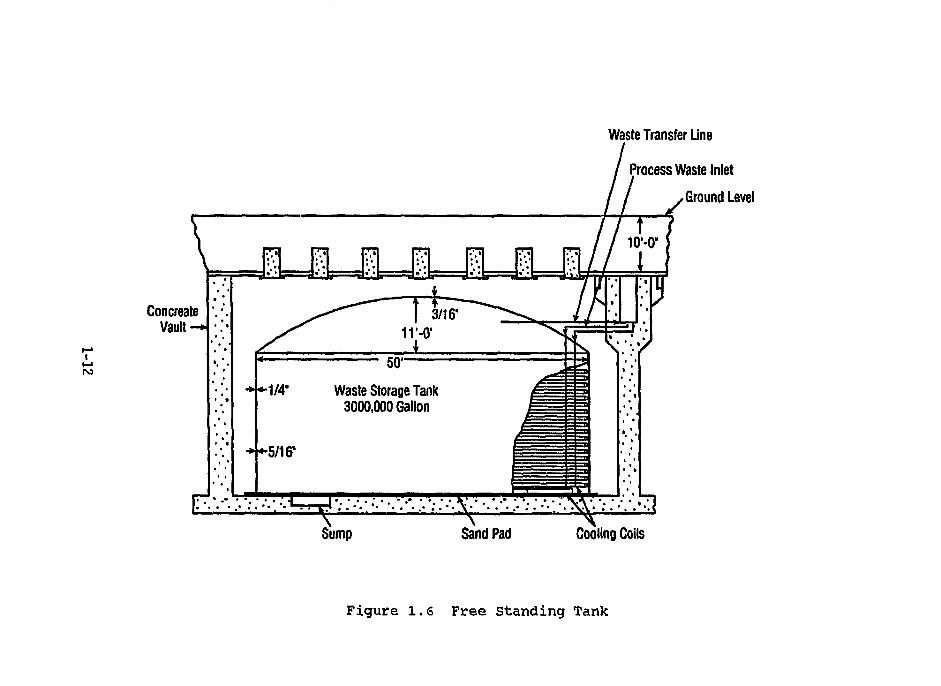
tank farm, the steel tanks containing wastes are free-standing

similar to above-ground tanks, and are enclosed by pre-cast or

cast-in-situ octagonal concrete vaults (Figure 1.6). The unique

details of all existing tanks are not necessarily illustrated in

these figures. Moreover, the design concept of future tanks may

be different. For example, in a new tank farm the primary tanks

may be built on a common footing enclosed by a large concrete

vault or can have a superstructure such as a weather enclosure.

In order to satisfy the confinement regulation, all new tanks

are expected to be designed as double-shell structures.

The entire tank structure is below the ground surface with a

soil cover up to 10 feet. Most tanks can contain approximately

one million gallons of waste. The tank diameter is in the range

of 75-80 feet and the maximum height of the iiquid waste is 30-

40 feet. There are a few smaller tanks. For example, there are

tanks with a capacity of 750,000, 300,000 or 55,000 gallons

each.

On the other hand, bin sets are used to store processed granular

waste such as calcined products. A bin set consists of a

cluster of long steel cylinders enclosed in a partially or

completely underground reinforced concrete cylindrical structure

(Figure 1.7).

1.3 OVERVIEW OF SEISMIC GUIDELINES

This report provides guidelines for treating earthquake loading

1-2

in the design and evaluation of HLW storage tanks. The

guidelines are applicable to the primary tank, secondary liner,

concrete vault, transfer piping and other components that are

required to maintain the confinement function of a tank farm.

Certain components are specifically addressed in this report and

general guidelines are provided for others. The guidelines

include a definition of the design basis earthquake ground

motion, simplified methods for determination of soil-structure

and liquid-structure interaction effects, analytical techniques

to compute the member forces, and the structural acceptance

criteria. The interpretation and use of the guidelines are

illustrated through an example included in this report.

The approach adopted for developing the guidelines is discussed

in Chapter 2. The guidelines are developed primarily for

double-shell tanks due to an immediate need for designing new

double-shell tanks. However, some of these guidelines are

generally applicable for single-shell tanks as well. Additional

work is required to address certain other aspects of the single-

shell tanks and various types of waste contents such as viscous

liquids and granular solid wastes. This report is expected to

be revised for inclusion of these additional criteria when they

become available.

The general criteria are described in Chapter 3. The seismic

criteria aim at achieving»a desired performance goal (e.g.,

confinement of HLW) expressed in probabilistic terms. This

performance goal is achieved by use of probabilistic seismic

hazard estimates in terms of a site-specific design response

spectrum. Thus, the design basis earthquake (DBE) ground motion

is determined by correlating probabilistic measures of the

performance goal and the seismic hazard. Once the DBE ground

motion is obtained, the remaining evaluations such as the

structural analysis and design are based on deterministic

methods. Acceptable material properties such as strength,

1-3

damping and inelastic energy absorption factors are also

discussed in Chapter 3. The appropriate load combinations and

the corresponding acceptance criteria are also described.

The criteria for evaluation of hydrodynaiaic effects in tanks are

described in Chapter 4. Simplified methods are presented for

both rigid and flexible tanks. Since for many of the double-

shell tanks the primary steel tank is supported at the top by

the concrete vault structure, formulation is provided for top-

constrained as well as free-standing tanks. Results are

applicable for wastes of various densities. However, it is

assumed that the waste is a non-viscous liquid (i.e., viscosity

same as water).

Chapter 5 provides an approach for determination of the seismic

capacity of flat-bottom vertical liquid storage tanks. Formulas

are presented for both anchored and unanchored tanks. Various

failure mechanisms of the tank components are considered. The

approach adopted for determination of the capacity requires

developing a nominal minimum ultimate strength capacity of the

tank and then applying appropriate strength reduction factors

that will provide factors of safety consistent with those

discussed in Chapter 3 and Appendix C.

The criteria for computation of soil pressure due to seismic

loads and in-vault response spectra that can be used to qualify

equipment are provided in Chapter 6. Simplified methods are

described for consideration of the soil-structure interaction

effect.

The above chapters concentrate on the tank structure.

Evaluation guidelines for underground transfer piping are

provided in Chapter 7. Guidelines for consideration of

potential for liquefaction are also included in this chapter.

Seismic qualification of equipment is discussed in Chapter 8.

1-4

The available qualification approaches are described and the

applicable standards are cited. The qualification level

required to satisfy the general seismic criteria presented in

Chapter 3 is also addressed.

The supporting technical information that was used in developing

the criteria is presented in the appendices. Appendix A expands

on the idea of the performance goal and demonstrates how a

desired goal can be achieved by using the basic seismic criteria

factors presented in Chapter 3. Two typical mean probabilistic

seismic hazard curves are used for illustration purposes.

Validation of the basic seismic design criteria presented in

Appendix A is demonstrated in Appendix B. Appendix C

demonstrates how the seismic criteria presented in this report

achieve a desired reduction of the ratio of the hazard frequency

and the seismic risk frequency. Results are presented for both

ductile and low-ductile failure modes. Appendix D includes

guidance on estimation of the inelastic energy absorption

factor. Appendix E provides formulations for tha membrane

solution of metal tanks constrained on top. The application of

the criteria in computation of the seismic response and tank

capacity is illustrated by considering an example in Appendix F.

Appendix G provides a set of coefficients that can be used for

soil-tank interaction analysis with the help of a lumped

parameter model.

1.4 NOTATION

A large number of symbols are used in the report to represent

various parameters. Attempts were made for being consistent

with notation used in national standards and codes and in common

literature. A set of general notation is used to denote major

parameters (such as force, moment, acceleration, etc.)- Certain

symbols represent more than one parameter; however, due to their

unique applications, they are expected to convey clear meanings.

The symbols used in various chapters either are made with

1-5

subscripts to the set of general notation and convey the same

general meaning or are completely new. In any event, the

symbols used in each chapter are separately listed and defined

in that chapter after the Reference Section and may not be

identical with symbols used in other chapters- This provides

the flexibility needed for consistency with commonly used

notation in a particular field of engineering, such as, seismic

hazards, fluid dynamics, soil mechanics and general structural

design. Certain minor symbols used for intermediate steps and

clearly defined in the text next to the equations are omitted

from the notation lists.

1-6

REFERENCES

1.1 DOE Order 6430.1A, "General Design Criteria", 1989.

1.2 "Design and Evaluation Guidelines for Department of Energy

Facilities Subjected to Natural Phenomena Hazards", UCRL-

15910, June 1990.

1-7

Concrete Dome

V8'-r.

ConcreteShell

45'-4"

Figure 1.1 A Typical Single-Shell Tank

Concrete Dome;; 7--0-.

55'-0" j^Steel Liner1

^Primary Tank2'-6" Annular Space

75"-0" Diameter

ConcreteShe"

. » . ' . • . . J . - .y i • J . y : • • • ! ' ! -r- • ••• ' • r-' •

Insulating Concrete

Figure 1.2 A Typical Double-Shell Tank

1-8

W 4'-0"Roof

r

33'-0"

wAir Space

. Cooling* Coils

Air Slots

2'-6"Wall Lr-R" Base Slab

85-0"

Secondary Liner •

Primary Liner-

6" Insulating Concrete

Figure 1.3 Tank with a Central Column

1-9

1'-10" Roof s9'-0"

V-10"Wall

24>-6l

12,2-0" O.D^Columns

*-21-6" Base Slab75'-0" •

\ "•Cover

VTank

SteelPan-

Figure 1.4 Tank with Concentric Columns

1-10

SeparationWith PVC

Water Stop

Upper Floor

ShieldStructure

/Removable/ Roof

Pre-EngineeredMetal Building

Soil Backfill

Reinforced Concrete

,/„>„„,,,

=£1

Pile Foundation

Figure 1.5 Tank with Concentric columns and Other Superstructures

ConcreateVault — I

•1/4"

50-

Waste Storage Tank3000,000 Gallon

Sump Sand Pad

Waste Transfer Une

Process Waste Inlet

s Ground Level

Cooling Coils

Figure 1.6 Free Standing Tank

Annular Steel Cylinders(51-0"1.D.,131-6"O.D.,681-0"H)

—Ground Level

Concrete Enclosure

Figure 1.7 A Typical Bin Set

1-13

CHAPTER 2

CONSIDERATIONS IN DEVELOPMENT OF GUIDELINES

2.1 INTRODUCTION

The principal philosophy that was considered in developing the

seismic design and evaluation criteria is to make maximum use of

the existing guidelines. DOE Order 6430.1A (Reference 2.1)

provides a set of general design criteria for the DOE

facilities. UCRL-15910 (Reference 2.2) provides specific

guidelines for design and evaluation of DOE facilities due to

earthquake and other natural phenomena such as wind and flood.

The graded approach adopted in UCRL-15910 is also used and

further expanded in this report for developing guidelines for

the tanks. Other analysis methods, design details and

acceptance criteria delineated in the UCRL document are used to

the extent they are applicable to the underground tanks. UCRL-

15910 is intended for general DOE facilities and not

specifically prepared for the tanks. Therefore, the next step

in the criteria development is to address the special features

of the underground tank and bin structures and identify the

technical issues that are not addressed by the existing

guidelines. The final step in the criteria development is to

address the technical issues that have been identified to be

unique for the underground tanks and combine the resolutions

with the existing guidelines. This chapter contains discussions

on the various criteria development steps as discussed above.

2.2 TECHNICAL ISSUES

Most of the technical issues that were considered for

development of the seismic guidelines are due to unique

structural and dynamic features of the underground tanks.

Although seismic evaluation techniques for aboveground tanks

have greatly advanced since the mid-1970's, and the design

2-1

criteria for these tanks are available, evaluation guidelines

for underground tanks are relatively scarce. There are

diversities of the tank designs in the DOE tank farms. For

example, some tanks are free-standing, some are partially

connected to the encasing concrete vaults and some use the

concrete vaults as a partial confinement barrier. In addition,

the waste contents in many tanks are not necessarily uniform and

not completely in the liquid state. Moreover, in many tanks the

waste products are believed to have settled forming layers near

the bottom. Therefore, the fluid-tank interaction methods

available for a dynamic analysis may not be directly applicable

to the HLW storage tanks. Furthermore, for certain tanks, crust

formation may not allow sloshing as assumed in standard

hydrodynamic load calculation methods. These special design

features and waste characteristics of the waste storage tanks

are not addressed in the existing literature.

The above issues were considered in developing the guidelines

presented in this report. The evaluation techniques for above-

ground tanks were extended and supplemented with specific design

considerations for the underground tanks. Some additional

technical issues were considered in this report for development

of the criteria since certain guidelines recommended in existing

documents such as UCRL-15910 would require updating to

incorporate lessons learned from recent studies in these areas.

These technical issues and the extent to which they are

addressed by the guidelines presented in this report are briefly

discussed in the following paragraphs. A further elaboration of

some of these issues is included in the subsequent chapters

where the guidelines are provided.

Site-Specific Hazard Curves - The current version of UCRL-15910

(Reference 2.1) recommends the use of site-specific hazard

curves for moderate and high hazard facilities, as does the DOE

"Interim Position" (Reference 2.3). However, UCRL-15910 permits

2-2

the use of the hazard estimates published in UCRL-53582

(Reference 2.4) for this purpose; but the guidelines presented

in this report require more recent hazard curves for HLW storage

tanks.

Soil Pressure - Since the tank structures are underground,

computation of the soil pressure on tank walls due to an

earthquake is an important element of the seismic evaluation.

Simplified methods were developed and are presented in this

report to determine the soil pressure including soil-structure

interaction effects. The simplified methods are based on lumped

parameter soil-structure-interaction models that have been used

extensively and successfully in seismic response analyses of

nuclear power plant facilities. However, the degree of

applicability of these models to the broad vaults of relatively

small height-to-radius ratios has not yet adequately been

assessed. Studies are currently underway to make this

assessment and, if necessary, to recommend appropriate

improvements.

Liquid Dynamic Loads - The pressure loads in cantilever tanks

due to water-type liquid can be determined by use of classical

solution techniques available in the literature. However, most

of the existing HLW steel tanks are unanchored at the base and

some are attached to the concrete enclosure on top. In order to

address such special characteristics, techniques were developed

for solution of top-constrained tanks and are described in the

report. The liquid wastes in most HLW storage tanks contain

suspended solids and, in many instances, become viscous or even

semi-solid materials if remain stored for a long time. The

density of the waste product typically varies over the depth as

a result of chemical reaction, crystallization and settling of

suspended solid particles. The formulation presented in this

report was derived for non-viscous uniform water-type liquids.

Viscous liquids are expected to manifest higher damping, and

2-3

produce lower sloshing and a greater liquid mass participating

in the impulsive mode. A sufficiently viscous liquid may even

transfer shear directly to the base. An analytical study

indicates that for liquids with viscosity up to 10,000

centipoise (cP)* the change in the liquid dynamic

characteristics is insignificant (Reference 2.5). The

applicability of the results to other waste characteristics will

be addressed by a future revision of this report.

Unanchored Tanks - As mentioned above, available classical

methods provide solution only of anchored tanks. The evaluation

of the seismic demand for unanchored tanks is considerably more

complex than for anchored systems, and the available methods of

analysis have not yet reached the levels of sophistication and

simplicity required for design applications. The seismic

response of the tank-liquid system in this document is computed

on the assumption that the tank is anchored at the base so that

it cannot slide or uplift. On the other hand, the seismic

capacity of the tank is evaluated for both anchored and

unanchored conditions, giving due regard to the nonlinear

resistance of the uplifting base. The combination of approaches

employed herein is believed to be sufficiently accurate for

design of both anchored and unanchored tanks and to lead to

conservative results.

Single-Shell Tanks - As described in Chapter 1, the concrete

enclosure of a single-shell tank retains the soil pressure as

well as contains the liquid waste. Thus, the concrete wall is

subjected to two opposing static pressure loads. However, in a

dynamic situation, the time phasing of these two pressure

components will determine whether they should be additive. This

aspect was not addressed in this report and requires further

*It is believed that a viscosity level of 10,000 cP represents an upper-boundvalue for the currently available liquids in many tank farms. The sludge atthe bottom of the tank, of course, can have a higher viscosity level andcould be considered as an elastic solid.

2-4

study. However, a design based on two separate considerations,

namely the soil pressure without the liquid pressure and the

liquid pressure without the soil pressure will be conservative.

This will be further discussed in a subsequent revision to this

report.

Granular Materials in Bins - Bins contain a granular material

obtained as a result of processing the liquid waste. This

material will produce dynamic pressure in a bin to some extent

similar to the hydrodynamic (impulsive) pressure in a tank.

However, a part of the inertia load of the bin content can be

transferred directly to the base. This aspect is not addressed

in this report and requires further study. However, in the

absence of a more refined set of criteria, the mass of the

entire quantity of the granular material can be conservatively

used to determine the dynamic pressure on the bin walls.

Underground Piping - Acceptance criteria for underground piping

are not explicitly discussed in current versions of available

piping codes. Procedures to evaluate stresses and strains

induced in underground piping and conduit from seismic effects

together with criteria to be used as a basis for acceptance are

presented in this report. Analysis procedures to be used to

assess both transient effects due to wave passage and support

point movements as well as long term permanent ground

displacements are considered in the evaluation. Modifications

to current procedures have been recommended to include seismic

effects within the criteria. Since stresses induced in

underground piping are considered as self-limiting by the

induced ground displacements, these modifications have been

based on consideration of seismic-induced stresses as secondary

and modifications to the acceptance criteria made to those

sections of the applicable codes treating these load types.

2-5

REFERENCES

2.1 DOE Order 6430.1A, "General Design Criteria," 1989.

2.2 "Design and Evaluation on Guidelines for Department of

Energy Facilities Subjected to Natural Phenomena Hazards,"

UCRL-15910, June 1990.

2.3 Interim Standard on "Use of Lawrence Livermore National

Laboratory and Electric Power Research Institute

Probabilistic Seismic Hazard Curves," Department of Energy

Seismic Working Group, Issued in March 1992.

2.4 Natural Phenomena Hazards Modeling Project: "Seismic

Hazards for Department of Energy Sites," UCRL-53582, Rev.

1, 1984.

2.5 "Effect of Viscosity on Seismic Response of Waste Storage

Tanks," Argonne National Laboratory Report ANL/RE-92/2,

June 1992.

2-6

CHAPTER 3

SEISMIC CRITERIA

3.1 INTRODUCTION

The objective of seismic design is to limit the likelihood of

unacceptable performance to a specified, low value. In this

document it is presumed that such a specified value (or, possibly,

suite of values for different components and structures) has been

provided to the seismic design team by those responsible for

overall project safety. This specified performance value depends

on factors such as the consequences of failure. Unfortunately,

future seismic ground motions, as well as structure and component

responses and capacities, are subject to varying degrees of

randomness and uncertainty, complicating the development of simple,

but accurate design procedures.

The engineering challenge is to achieve the performance goals,

i.e., the specified low probabilities of failure, in a practical,

cost-effective manner in the face of these multiple uncertainties.

This chapter provides the guidance to meet this objective

successfully.

After a discussion of the nature of the problem, Chapter 3 presents

a design or evaluation scheme that separates the problem into its

customary two phases: (1) the design basis earthquake ground

motion (DBE) and (2) the response and capacity criteria. The

former element is discussed in Section 3.3. Sections 3.4 to 3.9

present a set of practical response and capacity criteria that

together with the DBE defined in Section 3.3 will meet any

specified performance goal. Finally, Sections 3.10 and 3.11

(supported by Appendices A, B and C) present the basic criterion,

reasoning and analysis underlying these recommendations, as well as

permissible alternatives and generalizations that will achieve the

same performance goals. An application of these concepts and

3-1

generalizations will not only confirm the technical soundness of

the criteria and factors outlined in Sections 3.3 through 3.9, but

also lead to alternative analysis procedures that may prove more

effective in particular circumstances.

3.2 FUNDAMENTAL CONCEPTS

Elementary structural safety theory (e.g., Reference 3.1) as

practiced, for example, in seismic probabilistic risk assessments

(PRAs), requires that calculations of the failure probability for

a given design be conducted by a formal integration of the

probability distributions of the loads and capacities. This

probability can then be compared to the specified performance goal

to establish design adequacy. Such an integration will properly

reflect the uncertainties in both major elements of the problem.

Practical design demands simpler, more direct procedures, however.

The challenge in developing complete seismic criteria is to provide

that direct ("deterministic") analysis format while recognizing

both the probabilistic nature of the seismic hazard, as reflected

in the site's seismic hazard curve, and the documented variability

in dynamic responses, material properties, and structural

capacities. This challenge has been addressed with varying degrees

of success in the various available sets of seismic criteria.

Never before, however, have they been as explicitly developed as

they are in this document. The criteria below address directly the

following two major criteria-development difficulties: (1) the

seismic hazard curve varies significantly from site-to-site, both

in level and in shape, implying not only that the DBE- level must be

adjusted to the site, but also that any value of load factor (or

strength reduction factor) will imply different levels of risk

reduction at different sites; and (2) the total degree of

uncertainty in the capacity variable (associated with responses,

material strengths, and other factors) varies from location-to-

location (within a structure), from material-to-material, etc.

3-2

(This degree of uncertainty is commonly measured by a coefficient

of variation1 or similar dimensionless quantity.)

The procedure outlined in this chapter requires the specification

of two probability-related factors; together they will achieve the

specified performance goal, i.e., keep below PF, the allowable

(mean2) annual probability of unacceptable performance i.e., of

failure. The first factor is PH, the (mean) hazard or annual

probability of exceedance associated with a reference-level

earthquake3. The second is a risk or probability reduction factor,

RR to be associated with the acceptance criteria. The more

conservative these criteria the larger R,,. The values of PH and RBshould generally be selected such that:

PH= (Rs) iPF) (3-1}

This condition states in probabilistic terms, i.e., PF = PH/RR, the

obvious fact that the same safety can be achieved by many

combinations of design earthquake level and acceptance criteria,

provided that, when one is made less conservative, the other is

made appropriately more conservative in order to compensate.

1The coefficient of variation is defined as the standard deviation dividedby the mean. In seismic PRA analysis it is common to use, instead, the standarddeviation of the natural log of the variable, denoted p. For p less than about.0.3 the two coefficients are comparable in numerical value.

2As is common elsewhere (e.g., in the NRC Quantitative Safety Goals), weassume that the mean probability of failure will be specified. This implies thatthe uncertainty in this probability induced by currently limited data andprofessional knowledge (i.e., "epistemic uncertainty" as distinct from naturalrandomness or "aleatory" uncertainty) will be addressed by averaging over thatuncertainty. This uncertainty in seismic hazard curves is unusually large; itis captured in these criteria by using mean hazard curves. This mean is theaverage over the uncertainty in the hazard (probability) estimate. See Ref.3.13.

3We avoid here calling this earthquake level the Design Basis Earthquake,DBE, because, as will be seen in Section 3.3, while in some cases PH willdirectly define the DBE level, in others, an alternative, somewhat larger levelwill be necessary for the DBE level in order to achieve the performance goal.

3-3

It is presumed here, recall, that the seismic engineering team has

been given a value for PF, the performance goal. This value may

depend on the implications of the failure of the component, the

redundancy of the system, the marginal cost of strengthening the

component (versus another parallel component in the same system),

the remaining design life, etc. This performance goal ultimately

reflects the safety goals of the DOE (References 3.2 and 3.3).

The procedures in this document grant the flexibility of selecting

one or more pairs of values of PH and R,, to meet the goal, PF.

Typical values of RR considered are 5, 10, and 20. One advantage*,

of this flexibility is that the engineer can keep the same seismic

input level while consistently and easily adjusting the acceptance

criteria for components with different performance goals (within a

factor of 4, at least) . Alternatively, one can keep the same

criteria and adjust the earthquake.

Readers familiar with the DOE seismic criteria in the UCRL-15910

(Reference 3.4) will recognize this general format. In that

document performance goals (PF values) of 10"5 to 2X10"4 are

suggested for the more critical facilities. The document then

defines conservative seismic acceptance criteria aimed at achieving

risk reduction factors, RR, of about 5; 10, and 20. The users are

free to choose whichever set of criteria they wish. Reference 3.4

then recommends establishing the DBE by entering the seismic hazard

curves at an annual probability of exceedance of PH = (RR) (PF) . For

example, if the specified performance goal for a structure or

component is 10'5 and the selected set of acceptance criteria are

associated with an RR of 20, then the DBE should be that with an

annual probability of exceedance of 2X1CT4 (i.e., a mean return

period of 5000 years). The criteria in this document follow this

same philosophy. They supplement UCRL-15910 by providing criteria

and procedures for underground high-level waste storage tanks.

They also amplify UCRL-15910 by providing a more explicit, rigorous

basis for the specification- of the acceptance criteria and the

3-4

selection of the DBE; the development of this basis has

demonstrated the need to make certain refinements in the UCRL-15910

process. These developments insure, for example, that the

procedures are consistent over a broader range of hazard curve

shapes. It is expected that these improvements will be made in a

forthcoming revision of UCRL-15910.

Once the values of PH and RR have been established, the design or

evaluation of an existing component or structure follows

straightforward procedures. Section 3.3 details the selection of

the DBE earthquake consistent with PH (and, possibly RH, as will be

seen). .The seismic acceptance process may have one of various

forms. While more general processes are possible (see, Sections

3.10 and 3.11), the bulk of this chapter (Sections 3.4 to 3.9) is

dedicated to a conventional process based on deterministic factors4

and pseudo-linear analysis. One of these factors depends

explicitly on RR* While the procedure in Sections 3.4 and 3.9 has

been chosen because of its familiarity to those experienced in

seismic design..,and evaluation of commercial nuclear power plants

and other critical facilities, certain of the factors and details

have been adjusted by the authors to better approximate the

specified RR factors.

The primary steps in the procedure outlined in Sections 3.4 to 3.9

are:

A. Perform a linear e las t ic seismic response analysis for the DBE

ground motion to determine the elastic-computed seismic demand

Dse in accordance with Sections 3.4 and 3.5.

"By "deterministic" it is meant that for simplicity the specification of thevalues of the coefficients of variation and even, largely, particular percentilesis avoided. That this can be done without significant loss of generality oraccuracy is one of the facts demonstrated is this document, in appendices to becited.

3-5

B. Establish the code ultimate capacities Cc for all relevant

failure modes for each component being evaluated in accordance

with Sections 3.6 and 3.7.

C. For each failure mode of each component define the maximum

permissible inelastic energy absorption factor F^ by which the

elastic-computed seismic demand may exceed the code ultimate

capacity in accordance with Section 3.9.

D. Divide the elastic-computed seismic demand Dse by the

appropriate inelastic energy absorption factor FpD and multiply

by a seismic load factor Ls to define an inelastic-factored

seismic demand Dsi. This inelastic-factored seismic demand Dsl

is then combined with the "best-estimate" of the concurrent

non-seismic demands Dns to obtain a total inelastic-factored

demand Dti which must be less than the code ultimate capacity

Cc. This step is defined by Equation 3.4 through 3.6 of

Section 3.8.

The criteria presented are primarily based upon the judgment and

experience of the authors as being appropriate to roughly achieve

these seismic risk reductions. However, great rigor or

quantitative accuracy in achieving these seismic risk reduction

factors should not be implied. The factors merely served as target

goals in developing the criteria.

The seismic criteria presented herein are considered to be

sufficiently conservative to guard against damage from subsequent

aftershocks with ground motion less than the DBE.

Although it is envisioned that most users will prefer to follow the

deterministic pseudo-linear seismic evaluation procedure of

Sections 3.4 through 3.9 as outlined in the above four steps, a

more general basic seismic criterion and a general approach to

demonstrate compliance are presented in Section 3.10 in terms of an

acceptable probability of failure capacity. This basic seismic

3-6

criterion and alternate general approach to demonstrate compliance

are presented for two reasons:

1. To enable the user to define more sophisticated alternate

acceptance criteria than those presented in Sections 3.4

through 3.9 when the user has a sufficient basis to develop

and defend these alternate criteria.

2. To provide a basis upon which the seismic criteria of Section

3.4 through 3,9 were developed.

Lastly, Section 3.11, together with Appendix C, uses this basic

seismic criterion of Section 3.10 to benchmark the adequacy of the

factors used in the deterministic pseudo-linear seismic evaluation

procedure defined in Sections 3.4 through 3^9.

3.3 DESIGN BASIS EARTHQUAKE GROUND MOTION

3.3.1 Probabilistic Definition of Ground Motion

Given a seismic hazard curve for the site, such as the example in

Figure 3.1, it is straightforward to enter the curve at the value

PH (which equals RR PF) and read off the corresponding level of the

ground motion parameter [which is peak ground •acceleration (PGA) in

Figure 3.1]. For example, if PF is specified to be 10~5 and Rp is

selected to be 10, then PH is 10"4, and the DBE PGA is 0.3g at the

sites characterized by Figure 3.1. This is the same simple

procedure used in UCRL-15910.

It has been confirmed in the development of this document that this

procedure is adequate provided the shap& of the hazard curve is

close to that in Figure 3.1. In particular, the simple procedure

is adequate provided that in the range of interest, i.e., in the

10"4 to 10~5 range for high-level waste storage, the shape of the

curve is such that reduction in PH by an order of magnitude, e.g.,

10"4 to 10~5, leads to approximately a doubling of the ground motion

level.

3-7

An adjustment to the procedure is required, however, if this

approximate doubling does not characterize the site's hazard curve.

To make this modification a ground motion ratio, AB,- is introduced

as follows:

AR = .fatisr (3.2)aPH

in which aPH is the ground motion level at the exceedance frequency,

PH, at which the DBE is to be defined, and a0 1PH is the ground

motion level corresponding to a factor of ten reduction in this

annual exceedance frequency. For example, if it is recommended

that the DBE be defined at the 2X10"4 annual exceedance frequency,

AR is the ratio of ground motion at 2xlO~5 to that at 2X1CT4. For

Figure 3.1, AR = 0.5g/0.24g = 2.08, which is close to two.

This ratio AR may sometimes differ significantly from two. Figure

3.2 presents two representative probabilistic seismic hazard curves

expressed in terms of mean annual probability of exceedance versus

peak ground acceleration. Curve A represents a hazard estimate for

a western U.S. site. Curve B represents a typical hazard estimate

for an eastern (lower seismicity) site. For Curve A (the western

site), AR is 2.0 and 1.67 over the 10"3 to 10"4, and the 10~4 to 10"5

ranges, respectively. For curve B (the eastern site), AR is 2.31

and 2.13 over these same ranges. These results are typical. For

western U.S. (or higher seismicity) sites, the ratios for mean

hazard curves have been seen to range from about 2.0 to as low as

about 1.5 within the probability range from 10"3 to 10~5. For

eastern U.S. (or lower seismicity sites), the corresponding ARvalues usually range from about 2.0 to as high as about 3.75.

Furthermore, as seen in the examples, at any one site, AR is not

constant over probability ranges that differ by an order of

magnitude; AR reduces as the exceedance probability is lowered.

Because of this fact adjustments may have to be made for some

components whose PF and/or PH values differ.

3-8

As will be discussed in Section 3.10, AR ratios ranging from 1.5 to

3.75 can be accurately and slightly conservatively accommodated by

defining the DBE as the larger of aPH and faaPF, in which aPH and aPF

are the ground motion levels at the seismic hazard probability, PH,

and performance goal probability, PF, respectively, and in which fa

is an empirically derived adjustment factor defined as 0.45, 0.50,

and 0.55 for RR = 20, 10, and 5, respectively. Symbolically,

DBE > aPH (3.3a)

DBE > fa aPF (3.3b)

20105

0.450.500.55

It is expected that AR will virtually always lie within the range

of 1.5 to 3.75. However, even if An lies outside this range, the

larger of the results from Equations 3.3a and 3.3b should be used

to define the DBE ground motions.

Table 3.1 presents some example applications of Equations 3.3a and

3.3b for both the Curve A and Curve B probabilistic hazard curves

shown in Figure 3.2. For use in these examples, the following peak

ground accelerations (PGA) can be read from Figure 3.2:

ExceedanceProbability

1 x 10 3

2 x 10"1 x 104

1 x 105

PGA (g)

Curve A

0.300.500.601.00

Curve B

0.130.240.300.64

3.3.2 Design Basis Earthquake Response Spectra

The DBE ground motion at the site shall be defined in terms of

smooth and broad frequency content response spectra in the

3-9

horizontal and vertical directions defined at a specific control

point. In most cases, the control point should be on the free

ground surface. However, in some cases i t might be preferable

to define the DBE response spectra at some other locations. One

such case is when a soft (shear wave velocity less than 750

feet/second), shallow (depth less than 100 feet) soil layer at

the ground surface is underlain by much stiffer material. In

this case, the control point should be specified at the free

surface of an outcrop of this stiffer material. Wherever

specified, the breadth and amplification of the DBE response

spectra should be either consistent with or conservative for the

site soil profile, and facility embedment conditions.

Ideally, i t is desirable for the DBE response spectrum to be

defined by the mean uniform hazard response spectrum (UHS)

associated with the seismic hazard annual frequency of

exceedance specified in Section 3.2 above and Reference 3 • 4 over

the entire natural frequency range of interest (generally 0.5 to

40 Hz) . Currently, however, considerable controversy exists

concerning both the shape and amplitude of such mean UHS5.

First, many existing mean UHS shapes are not consistent with

response spectrum shapes derived from earthquake ground motion

recordings. The DBE response spectrum should be consistent in

shape with response spectrum shapes from ground motion recorded

5The UHS associated with using a specified mean hazard is not, precisely,the mean spectral velocity associated with a specified hazard. The distinctionis directly analogous to the difference between the regression of Y on X versusthat of X on Y. See any elementary statist ics text. Therefore we should perhapsuse the terms "mean" UHS, "mean" PGA, etc . , to denote the former values, i . e . ,those spectral or other values read from mean hazard curves. For simplicity,however, we shall drop the quotation marks. Incidentally, i t should beemphasized that mean here refers to averaging over uncertainty in the estimationof hazard/probability. These "mean" UHS are not to be confused with the meanspectrum given a specified magnitude and distance, or the mean spectrum given aspecified PGA. These two concepts, with counterparts such as median and 84percentile spectra, are very common in earthquake engineering; the means,medians, and 84-percentiles represent in these cases distribu'tions over repeatedevents or records, a variability included explicitly within the hazard analysis.

3-10

at similar sites for earthquakes with magnitudes and distances

similar to those which dominate the seismic hazard at the

specified annual frequency. Unless it can be demonstrated that

the mean UHS shape is consistent with the response spectrum

shapes obtained from appropriate ground motion records, mean UHS

should not be used.

Second, even for a specified ground motion parameter such as

peak ground acceleration (PGA) or peak ground velocity (PGV),

the estimate for a given mean hazard or exceedance probability,

PH, tends to be unstable between different predictors and tends

to be driven by extreme upper bound models. Mean ground motion

estimates should be used only when such estimates are stable.

Mean estimates outside the range of 1.3 to 1.7 times the median

estimate are likely to suffer from the above problems.

Because of these issues with regard to both mean estimates and

UHS, the Department of Energy has published a draft interim

position on the use of probabilistic seismic hazard estimates

(Reference 3.5). The following recommendations have been

adapted from Reference 3.5:

1. When a stable mean estimate of the PGA and PGV does not

exist, then a surrogate mean DBE PGA and PGV set at an

appropriate factor times their median estimates at the

appropriate seismic hazard annual frequency of exceedance

should be used. Reference 3.5 defines an approach which

may be used to obtain an acceptable median estimate from

existing eastern U.S. seismic hazard study results, and it

defines this surrogate median-to-mean factor.

2. The DBE response spectrum is then defined by a smooth,

deterministic, broad-frequency-content, median6 response

6The word median here refers to the median with respect to a suite ofrecords. See the previous footnote.

3-11

spectrum shape scaled so as to be anchored to the

surrogate mean DBE PGA and PGV values defined in Step 1.

Preferably, the median deterministic DBE response spectrum shape

should be site-specific and consistent with the expected

earthquake magnitudes, and distances, and the site soil profile

and embedment depths. Reference 3.5 provides an acceptable

approach for estimation of the earthquake magnitudes and

distances to be used in defining this median deterministic site-

specific response spectrum shape. When a site-specific response

spectrum shape is unavailable then a median standardized

spectral shape such as the spectral shape defined in NUREG/CR-

0098 (Reference 3.6) may be used so long as such a shape is

either reasonably consistent with or conservative for the site

conditions.

The median site-specific response spectrum shape may be derived

from any combination of the following:

a) the median response spectrum shape from a suite of actual

ground motion records associated with reasonably similar

magnitudes, distances, and site soil profiles.

b) regression equations defining median spectral

amplifications at various natural frequencies as a

function of the magnitude, distance, and soil profile.

c) band-width limited random vibration models benchmarked

against response spectra from actual ground motion records

associated with magnitudes, distances, and soil profiles

as sdmilar to the site as practical.

In some cases the mean DBE PGA and PGV may be associated with

different controlling earthquakes in which the PGA is controlled

by a lower magnitude local earthquake while the PGV is

controlled by a larger magnitude more distant earthquake. In

these cases it is preferable to develop separate DBE response

3-12

spectra for each of the two controlling earthquakes in lieu of

a single enveloped DBE response spectrum. This alternative is

particularly appropriate when site-specific spectra shapes are

used rather than a standardized spectral shape, and the site-

specific spectral shapes differ substantially for the two

controlling earthquakes. In this case, the local earthquake

spectral shape should be anchored to the mean DBE PGA, and the

more distant earthquake spectrum shape should be anchored to the

mean DBE PGV. Both spectra may then be used separately in the

seismic response analysis with the largest of the separately

computed responses being used to define the seismic demand. Of

course, alternately, the two DBE response spectra may be

enveloped by a single combined DBE response spectrum which is

used to define the seismic demand.

In addition, in order to define low frequency (below 1 Hz)

response or for the evaluation of underground piping, it may be

necessary to also define a mean DBE peak ground displacement

(PGD) . This PGD is likely to be controlled by a larger

magnitude earthquake at greater distance than the earthquake

which controlled the DBE PGV.

3.4 ANALYSIS OF SEISMIC DEMAND (RESPONSE)

It is anticipated that the seismic demand will generally be

estimated based upon linear response analyses. Sections 3.4

through 3.9 outline a set of acceptance criteria consistent with

this approach. (But see also Section 3.10.). DBE response

spectra arrived at in accordance with Section 3.3 should be used

as input to such analyses. Other than for the conservatism

specified in the DBE response spectra, the seismic response

analyses can be median centered (no intentional conservatism),

but with variation of some of the most uncertain parameters.

Seismic response analyses should be conducted in accordance with

the guidance contained in References 3.4 and 3.7 as amplified

upon and modified herein.

3-13

Best estimate structural models and material damping values

should be used. Best estimate material damping values are

provided in Section 3.5. However, a variation by approximately

plus/minus one standard deviation in both the natural frequency

of the structure model, and soil stiffness properties should be

incorporated into these analyses. In general, the structural

frequency uncertainty can be accommodated by use of a 30%

frequency uncertainty band either centered on the best estimate

frequency or skewed to the low frequency side when such skewness

is considered appropriate. Guidance on the appropriate

variation of soil stiffness properties is given in Section

3.3.1.7 of ASCE4.86 (Reference 3.7) and Section 3.7.2 of the

USNRC Standard Review Plan (Reference 3.8). The seismic demand,

Dse, should be obtained from the largest computed response within

these uncertainty bands. Great precision is unnecessary, and

this largest response can generally be estimated by considering

the following five cases:

1. Best estimate model (best estimate structural model

coupled with best estimate soil properties).

2. Best estimate model frequency shifted +15%.

3. Best estimate model frequency shifted -15%.

4. Best estimate structural model coupled with upper estimate

soil stiffness properties.

5. Best estimate structural model coupled with lower estimate

soil stiffness properties.

As noted above, it is sometimes preferable to skew the 30%

frequency uncertainty to the low frequency side and for these

situations, Cases 2 and 3 should be adjusted accordingly. Floor

spectra should be smooth (valleys filled in) envelopes from

these cases.

3-14

It is seldom necessary to analyze all five cases. When soil-

structure-interaction (SSI) effects are substantial, Cases 4 and

5 will lead to broader frequency shifting than will Cases 2 and

3 so that Cases 2 and 3 can be dropped. When SSI effects are

small, Cases 4 and 5 will be enveloped by Cases 2 and 3 and can

then be dropped.

3.5 DAMPING

Damping values recommended for dynamic analyses are presented in

Table 3.2 at three different response levels. These values may

be used unless lower damping values are specified in the

applicable construction code or standard specified by the

Department of Energy for the facility design. Response Level 3

corresponds to inelastic response where the elastically computed

total demand (seismic plus non-seismic) exceeds the capacity

limits defined herein (i.e., credit must be taken for the

inelastic energy absorption factor F M). When evaluating the

component, Response Level 3 damping may be used in elastic

response analyses independent of the state of response actually

reached, because such damping is expected to be reached prior to

component failure. When determining the input to subcomponents

mounted on a supporting structure, the damping value to be used

in elastic response analyses of the supporting structure to

define input to the subcomponent should be a function of the

response level reached in the majority of the seismic load

resisting elements of the supporting structure. Defining Dt as

the total elastic- computed demand (seismic Dse plus non-seismic

Dns) for the combined (three earthquake components) and enveloped

(frequency varied) results and Cc as the code strength capacity

(see Section 3.7) for the supporting structure, then the

appropriate Response Level damping can be estimated from the

following:

3-15

Response Level

3

2*

1*

Dt/Cc

> 1 .0

«0.5 to 1.0

< 0 . 5

•Consideration of these damping levels is required only inthe generation of floor or amplified response spectra tobe used as input to sub-components mounted on thesupporting structure.

The damping values presented in Table 3.2 are intended to be

best-estimate (median centered) damping values with no

intentional conservative bias for use in elastic response

analyses. Other damping values may be used when such values are

properly justified as best-estimate values. For example, in the

case of very high viscosity fluid, impulsive mode damping values

in excess of 4% are permissible for tanks.

Response Level 3 damping values are intended for use in elastic

response analyses coupled with the permissible inelastic energy

absorption factors F defined later. However, when a nonlinear

inelastic response analysis which explicitly incorporates the

hysteretic energy dissipation is performed, no higher than

Response Level 2 damping values should be used to avoid the

double-counting of this hysteretic energy dissipation which

would result from the use of Response Level 3 damping values.

3.6 MATERIAL STRENGTH PROPERTIES

For existing components, material strength properties should be

established at the 95% exceedance actual strength levels

associated with the time during the service life at which such

strengths are minimum. If strengths are expected to increase

during the service life, then the strength of an existing

component should be its value at the time the evaluation is

performed. If strengths are expected to degrade during the

3-16

service life, then strengths to be used in the evaluation should

be based upon estimated 95% exceedance strengths at the end of

the service life. Whenever possible, material strengths should

be based on 95% exceec'ance values estimated from tests of the

actual materials used at the facility. However, when such test

data are unavailable, then code minimum material strengths may

be used. If degradation is anticipated during the service life,

then these code minimum strengths should be further reduced to

account for such degradation (for example, long term thermal

effects on concrete). See Section 3.7 for additional discussion

on applicable code material strengths.

For new designs, material strength properties should be

established at the specified minimum value defined by the

applicable code or material standard. If degradation is

anticipated during the service life, then these code minimum

strengths should be further reduced to account for such

degradation.

3.7 CAPACITIES

In general, for load combinations which include the DBE loading,

capacities Cc to be used should be based upon code-specific

minimum ultimate or limit-state (e.g., yield or buckling)

capacity approaches coupled with material strength properties

specified in Section 3.6. For concrete, the ACI ultimate

strength approach with the appropriate capacity reduction

factor, 0, included as specified in either ACI318 (Reference

3.9) or ACI349 (Reference 3.10) should be used. For structural

steel, the AISC-LRFD (Reference 3.11) limit-state strength

approach with the appropriate capacity reduction factor, <p,

included is preferred. However, the AlSC-Plastic Design (Part

2, Reference 3.12 or Chapter N, Reference 3.13) maximum strength

approach may be used so long as the specified criteria are met.

The plastic design strengths can be taken as 1.7 times the

allowable stresses specified in Reference 3.12 or 3.13 unless

3-17

another factor is defined in the specified code. For ASME

Section III, Division 1 components, ASME Service Level D

(Reference 3.14) capacities should be used. In some cases,

functional failure modes may require lesser limits to be defined

(e.g., ASME Mechanical Equipment Performance Standard, Reference

3.15).

For existing facilities, in most cases, the capacity evaluation

equations should be based on the most current edition of the

appropriate code, particularly when the current edition is more

conservative than earlier editions. However, in some cases

(particularly with the ACI and ASME codes), current code

capacities may be more liberal than those specified at the time

the component was designed and fabricated, because fabrication

and material specification requirements have become more

stringent. In these later cases, current code capacities will

have to be reduced to account for the more relaxed fabrication

and material specifications that existed at the time of

fabrication. In all cases, when material strength properties

are based on code minimum material strengths, the code edition

enforced at the time the component was fabricated should be used

to define these code minimum material strengths.

If any material can be degraded during the service life, the

degraded material size and properties should be used for

estimation of the component capacity. For example, when

corrosion is likely during the service life, thicknesses should

be reduced by an appropriate corrosion allowance before

computing the code capacity.

A capacity approach acceptable for the seismic capacity

evaluation of unanchored and anchored flat-bottom liquid storage

tanks at the atmospheric pressure is presented in Chapter 5. It

is judged that for temperatures not exceeding 200°F, the thermal

effects need not be considered explicitly in such capacity

evaluations.

3-18

3.8 LOAD COMBINATIONS AND ACCEPTANCE CRITERIA

This section deals only with load combinations that include DBE

loadings. In many cases, other (non-seismic) load combinations

may control the design or evaluation of a component. These non-

seismic load combinations should be defined by other documents.

It is assumed herein that the DBE seismic demand, Dse, will be

computed by linear elastic analyses conducted in accordance with

the response criteria defined in Sections 3.3 through 3.5. This

elastic-computed seismic demand Dse should be modified by the

appropriate inelastic energy absorption factor FMD as defined in

Section 3.9 and by the appropriate seismic load factor Ls to

obtain an inelastic-factored seismic demand Dsl by:

D ~ (3.4)

The seismic load factor Ls is used to accommodate varying seismic

risk reduction factors RR and ranges as follows:

RR

20

10

5

1.15

1.00

0 .87(3.4a)

Note that this is the only factor that need be adjusted to

modify the acceptance criteria for different specified RR levels.

(Recall, however, that in some circumstances the DBE level may

be modified if RR changes; see Section 3.3.).

The total inelastic-factored demand Dti is then given by:

= Dn si (3-5)

where Dns represents the best-estimate of all non-seismic demands

expected to occur concurrently with the DBE. Equation 3.5

represents the DBE load-combinations equation. The seismic

3-19

capacity is adequate when the capacity Cc determined as defined

in Section 3.7 exceeds Dti, i.e.:

( 3 . 6 )

Equation 3.6 represents the seismic acceptance criterion

appropriate for the DBE.

No load factors are needed on Dns in Equation 3.5. The non-

seismic demand Dns should be defined at its best-estimate level

as opposed to an unlikely-to-exceed or conservative level. The

conservatism embodied in defining Cc, F^, and Dse are sufficient

to achieve the specified RH values without additional sources of

conservatism being required.

In some cases, such as a column under combined axial compression

and moment, the code capacity Cc is defined in terms of

interaction equations. Furthermore, the F^p for axial

compression defined in Section 3.9 is less than FpDM for flexure.

In this case, Equations 3.4 and 3.5 are separately entered to

establish the total inelastic demands Ptl and Mti for axial

compression and moment, respectively, i.e.:

Pti Pn. ' "ti *» ^ (3.7)r\iDP " rv.DM

The combination of Pti and Mti is entered into the code capacity

interaction equation to determine the adequacy of the seismic

design.

For ductile failure modes, non-seismic demands which are

relieved by small levels of inelastic distortion (such as

thermal and settlement stresses) do not have to be included in

Equation 3.5 for combination with the factored seismic inertial

force induced demand. However, for non-ductile failure modes,

3-20

these inelastic-relieved non-seismic stresses must still be

included. For example, if a wall capacity is controlled by

flexure, these inelastic-relieved non-seismic stresses do not

have to be added to the seismic demand D(1. However, if the wall

capacity is controlled by shear, they do have to be added. In

addition, seismic and non-seismic displacements and strains are

additive when checking displacement or strain criteria such as

for underground pipes (see Chapter 7).

As another example, many vertical cylindrical flat bottom high-

level waste storage tanks are restrained against longitudinal

(vertical) movement at both the top and bottom of the tank

walls. In many cases, the degree of longitudinal restraint is

uncertain and difficult to quantity. Therefore, the

longitudinal stresses set up in the tank walls are difficult to

determine, but can be bounded by the cases of full longitudinal

restraint and no longitudinal restraint. When fully restrained,

substantial longitudinal stresses occur in the tank walls due to

the following reasons:

1. Poisson's ratio induced longitudinal stresses resulting

from the circumferential (hoop) stresses induced by the

combination of hydrostatic and hydrodynamic fluid

pressures on the tank wall (See Chapter 4) . For all

practical problems, these Poisson's ratio induced

longitudinal stresses are tensile and are a small fraction

(about 30%) of the average peak hoop stress over the

height of the tank. They are easily relieved by a very

small amount of longitudinal straining in the cylindrical

shell or support relaxation.

2. Thermal expansion stresses. These longitudinal thermal

expansion stresses are compressive and may be large at

high temperatures. But, at metal temperatures not

exceeding 200°F the corresponding longitudinal compressive

strains are less than 0.15% and thus the stresses are

3-21

easily relieved by small amounts of inelastic straining or

bowing of the thin metal tank sidewalls.

In conclusion, for a ductile metal tank, both of the above two

longitudinal stresses are secondary and easily relieved by a

very small amount of nonlinear longitudinal straining (less than

0.15%). As such, neither of these computed elastic longitudinal

stress will reduce the seismic capacity of the tank, and neither

of them have to be combined with the primary seismic overturning

induced longitudinal stresses when defining Dti by Equation 3.5.

3.9 INELASTIC ENERGY ABSORPTION FACTOR

The inelastic energy absorption factor is defined as the amount

that the elastic-computed seismic demand may exceed the capacity

of a component without impairing the performance of the

component. Thus, the elastic-computed seismic demand Dse may be

factored by an inelastic energy absorption factor FpD as shown in

Equation 3.4 to obtain an inelastic factored seismic demand Dsi.

In order to achieve a ratio of the seismic hazard frequency to

the seismic risk frequency between 5 and 20, this inelastic

energy absorption factor FMD should be defined by:

F.D = F-5% (3.8)

where F ^ is the estimated inelastic energy absorption factor

associated with a permissible level of inelastic distortions

specified at about the 5% level, i.e., there is only a 5% chance

that F will be less than F^^.

It is always preferable to perform nonlinear analysis on the

structure or component being evaluated in order to estimate F ^

for use in Equation 3.8 to define F „. Some guidance on

estimating FM5% is given in Appendix D. However, such analyses

are often expensive and controversial. Therefore, a set of

standard values of F^ is provided in Table 3.3 for common

elements associated with underground high-level waste storage

tanks, and discussed in the remainder of this section.

3-22

Additional FM values are provided in Table 4.7 of Reference 3.4.

The FM values presented in Reference 3.4 for the Moderate Hazard

category may be used for Fv0. The FMD values presented in Table

3.3 or from Reference 3.4 may be used in lieu of performing

nonlinear analyses, so long as the following cautions are

observed.

The use of FpD values listed in Table 3.3 equal to 1.5 and

greater for concrete walls is conditional on extensive wall

cracking but stable wall behavior constituting acceptable wall

performance. If only minor wall cracking is acceptable, then Fp0

should be 1.0.

The FMD values listed in Table 3.3 for ductile failure modes

(i.e., greater than 1.0) assume that steel reinforcing bars,

metal tank shells and anchorage will remain ductile during the

component's entire service life. It is assumed that the metal

will retain at least a 6% uniaxial elongation strain capability

including the effects of welding. If this metal can become

embrittled at some time during the service life, F,,o values

should be 1.0.

In some cases reinforcement details in older facilities do not

satisfy the development length requirement of current codes

(References 3.9 and 3.10). In these instances the potential

exists for a ductile failure mode associated with yielding of

the reinforcement to become a more brittle mode associated with

bond failure. Data exist (Reference 3.16), however, indicating

that bond failure modes retain a reasonable amount of ductility

provided that the reinforcement is suitably confined within the

region of the potential bond failure. The confinement may be

provided by a cover of at least 2.5 bar diameters or by ties

(stirrups) spaced no further than 5 bar diameters apart. If

this confinement is provided a strength of the reinforcement

equal to the yield strength of the steel times the ratio of

actual to required development length may be used in the

3-23

capacity evaluations. In these cases the factor (F^) should be

limited to 1.0. If the confinement is not provided the

reinforcement should be omitted in the capacity evaluations.

The F^ values listed in Table 3.3 or from Reference 3.4 and the

acceptance criteria of Section 3.8 are based on the assumption

that the component will be removed from service after being

subject to ground motion in excess of the DBE response spectrum.

If a component is to remain in service after being subjected to

a DBE, particularly when stress corrosion cracking is a major

concern, FM0 should be 1.0 and either the seismic load factor Ls

in Equation 3.4 may have to be increased or the capacity Cc may

have to be reduced in order to maintain the seismic margin

defined in Section 3.10.

For low-ductility failure modes such as axial compression or

shear in concrete walls or columns and wall-to-diaphragm, wall-

to-column, or column-to-base connections, the F^ values listed

in Table 3.3 are 1.0. In most cases, such stringent limits can

be relaxed somewhat,as described below, because most components

also have a ductile failure mode which when reached is likely to

limit the demand in the low-ductility failure modes. Unless the

component has a seismic capacity in the ductile failure mode

significantly in excess of its required capacity, inelastic

distortions in this ductile failure mode will likely limit the

factored seismic Dsi in the low-ductility failure modes to levels

less than those given by Equation 3.4 with the FM0 values given

by Table 3.3. Since greater conservatism exists in code

capacities Cc for low-ductility failure modes than for ductile

failure modes, the failure will be controlled by the ductile

failure mode so long as the low-ductility failure mode code

capacity is at least equal to the ductile failure mode capacity.

Thus, for low-ductility failure modes, the factored seismic

demand Dsi can be limited to the lesser of the following:

1. Dsl given by Equation 3.4 using FM0 from Table 3.3, or

3-24

2. Dtl = Cc - Dns computed for the ductile failure mode, where

Cc is the ductile failure mode code capacity.

Therefore, for example, connections do not have to be designed

to have code capacities Cc greater than the code capacities Cc of

the members being connected, or the total factored demand Dtl

given by Equations 3.4 and 3.5 and Table 3.3, whichever is less.

Similarly, the code shear capacity of a wall does not have to

exceed the total shear load which can be supported by the wall

at the code flexural capacity of the wall. Finally, the

horizontal seismic-induced axial force in a moment frame column

can be limited to the axial force which can be transmitted to

the column when a full plastic hinge mechanism develops in the

frame where the plastic hinge capacities are defined by the code

ultimate flexural capacities.

When the dominant response frequency (generally the fundamental

frequency) of the component is greater than the frequency at

which the input spectral acceleration is maximum, the cautions

contained in Section 4.2.3 and illustrated in Figure 4-4 of

Reference 3.4 remain in effect. In this case, the factored

seismic demand Dsi may be computed from any of the following

three approaches:

1. The maximum spectral acceleration shall be used to compute

the elastic response of the dominant response mode in lieu

of the lesser input spectral acceleration corresponding to

the frequency of this mode. In this case, the FpD values

listed in Table 3.3 or Reference 3.1 may be used.

2. The lesser spectral acceleration corresponding to the

modal frequency of the dominant response mode may be used

together with FMD values of 1.0.

3. The spectral acceleration corresponding to the modal

frequency of the dominant response may be used together

3-25

with FM0 values based on F ^ computed from nonlinear

analyses in accordance with guidance given in Appendix D.

This approach is the most accurate and least conservative

approach, but requires more effort.

The DBE response spectra defined in accordance with Section 3.3

are elastic response spectra which may be directly used to

compute the elastic-computed seismic demand which is then

divided by F^ to obtain an inelastic-factored seismic demand.

However, some engineers prefer to reverse the order of these

steps by first dividing the elastic response spectra by F^ to

obtain inelastic response spectra which may be directly used to

compute the inelastic-factored seismic demand. This approach is

also permitted so long as it is performed consistent with the

use of F^ as described herein.

One way to obtain this consistency is to first multiply the

elastic DBE response spectra by the seismic load factor Ls

defined by Equation 3.4a to obtain the load-factored elastic DBE

response spectra. Next, at all frequencies equal or less than

the frequencies at which the input spectrum is maximum, these

load-factored elastic DBE response spectra are divided by F ^ to

obtain the inelastic-factored spectra. At all higher

frequencies, the inelastic-factored spectral accelerations are

defined by the lesser of either the load-factored elastic

spectral acceleration at that frequency, or the maximum load-

factored elastic spectral acceleration divided by F(l5%.

Alternately, frequency dependent Fv5H obtained in accordance with

the guidance given in Appendix D and appropriate references such

as References D.I through D.6 of Appendix D may be used at all

frequencies to obtain the inelastic-factored response spectra

from the load-factored elastic response spectra. This method

becomes more complicated when different failure modes with

differing Fv5H are present.

3-26

This completes the specification of a set of seismic criteria

that will satisfy the performance goal PF through first the

introduction of PH and RR, followed by the determination of the

DBE and acceptance criteria, as outlined in Sections 3.3 through

3.9.

3.10 THE BASIC SEISMIC CRITERION AND THE GENERAL APPROACH TO

COMPLIANCE

The basic seismic criterion and the more general approach to

compliance presented in this section are needed for only the

following reasons:

1. To enable the user to define more sophisticated alternate

acceptance criteria than those presented in Sections 3.4

through 3.9, when the user has a sufficient basis to

develop and defend these alternate criteria, and

2. To provide the quantitative basis (in conjunction with

Section 3.11) upon which the seismic criteria of Sections

3.4 through 3.9 were developed.

The application of the deterministic, pseudo-linear seismic

evaluation procedure defined in Sections 3.4 through 3.9 does

not require the use of any of the material presented in Sections

3.10 and 3.11.

3.10.1 The Basic Seismic Criterion

For probabilistic seismic hazard curves such as those shown in

Figures 3.1 and 3.2, it is demonstrated in Appendix A that risk

reduction factors RR of 20, 10 and 5 are closely obtained when:

C10% ;> 1.5LJDBE) (3*9)

In this, the basic seismic criterion. C10% represents the 10%

seismic input percentile level, i.e., the level at which a 10%

3-27

probability of failure is estimated, and L, depends on Rn as

follows:

RR

20

10

5

1.15

1.00

0.87

(3.9a)

Notice that this single "basic" criterion (Equation 3.9)

compares capacity and demand in ground motion terms, rather than

in force, stress, or deformation terms, as is implied in

Sections 3.4 to 3.9. The non-seismic demands are implicitly

included here within C10%.

Appendix A demonstrates that the basic seismic criterion defined

by Equation 3.9 (with Equation 3.9a) is appropriate for a wide

range of hazard curves with different shapes, i.e., with a wide

variation ot ground motion ratios AR (defined by Equation 3.2)

when the DBE ground motion is defined as the larger of the

values given by Equations 3.3a and 3.3b. This demonstration

covers the practical range of AR ratios from 1.5 to 3.75.

However, the basic criterion Equation 3.9 (with Equation 3.9a),

coupled with the DBE defined by Equations 3.3a and 3.3b, can be

extended beyond this range of AR values with generally increasing

conservatism.

Using numerical convolution of hazard and fragility curves,

Appendix B validates the applicability of Equation 3.9 (with

Equatin 3..9a) for several cases with the hazard curves given in

Figure 3.2.

3.10.2 The General Approach to Compliance

The most general approach to demonstrate compliance with the

3-28

above basic seismic criterion is as follows,

performance criterion PF and the preferred 1^:

Given the

20

10

5

Ls

1.15

1.00

0.87

Fe

1 . 7

1 . 5

1 . 3

1. Establish the DBE ground motion in accordance with the

guidance of Section 3.3.

2. Define a Scaled Design Basis Earthquake (SDBE) ground

motion by increasing the DBE ground motion by an

earthquake adjustment factor F. defined by:

SDBE = (Fe) (DBE) (3.10)

in which

F, = 1.5 L, (3.11)

where Ls is the appropriate seismic load factor from

Section 3.10.1 for the selected seismic risk reduction

factor RR. Thus, one obtains the following values of Fe:

(3.11a)

3. Perform sufficient linear analyses, nonlinear analyses,

testing, etc., to reasonably determine that for the

combination of the SDBE with the best-estimate of the

concurrent non-seismic loads there is less than about a

10% probability of unacceptable performance.

Any seismic evaluation approach which is consistent with the

above three steps is acceptable.

3.11 BENCHMARKING DETERMINISTIC SEISMIC EVALUATION PROCEDURES

AGAINST THE BASIC SEISMIC CRITERION

The basic criterion Equation 3.9 (with Equation 3.9a) defines

the necessary overall conservatism that must be input into any

seismic evaluation procedure in order to achieve the desired

performance goal probability PF. The DBE has a PH consistent

3-29

with PF and RH. Recall for the seismic hazard curve with the

shape of Figure 3.1,RR = PH/ PF (3.12)

The necessary overall conservatism to satisfy Equation 3.9 could

have been introduced into Steps A through D by any of a variety

of combinations of values or factors in the deterministic

pseudo-linear seismic evaluation procedure described in Section

3.1 and defined in detail in Sections 3.4 through 3.9. The

deterministic procedure defined in Section 3.4 through 3.9 was

chosen because it closely follows existing practices for the

seismic design of critical facilities.

In this approach, very little conservatism has been introduced

in the computation of the elastic-computed seismic demand

(Section 3.4). Best estimate structural models and material

damping are used. It has been found that introducing

conservatism into the elastic-computed demand analysis

introduces a highly variable factor of conservatism across the

entire spectrum of natural frequencies and locations within a

structure. This variation makes it difficult to achieve a

specified target risk reduction ratio, RR. Reasonable variation

in structure and soil stiffness properties are, however,

considered and the maximum computed seismic demand over this

uncertainty variation is used to represent the elastic-computed

seismic demand. It is estimated that enveloping the effects of

these stiffness variations results in less than a 25% chance of

the elastic-computed response being exceeded given the

occurrence of the DBE.

On the other hand, considerable conservatism has been introduced

in the specified capacity by using minimum code ultimate

capacities (including code specified strength reduction factors)

coupled with 95% exceedance or code specified material strengths

(Sections 3.6 and 3.7). For ductile failure modes, it is

expected that the specified capacities will have at least a 98%

probability of being exceeded by the actual capacities. For

3-30

brittle failure modes, code capacities contain even greater

conservatism; the code capacity typically being about half of

the median (or "best-estimate") capacity.

Also considerable conservatism is introduced in the specified

maximum permissible inelastic energy absorption factor by which

the elastic-computed seismic demand is divided to obtain the

inelastic-factored seismic demand (Section 3.9). The

permissible inelastic energy absorption factor F^ is

conservatively established at its value associated with

inelastic distortions corresponding to about a 5% failure

probability.

In addition, a seismic load factor Ls is introduced in Equation

3.4 used to define the inelastic-factored seismic demand so as

to accommodate a range of seismic risk reduction ratios ranging

from 20 to 5. The values of the seismic load factor Ls and the

required degree of conservatism for the permissible inelastic

energy absorption factor F^ were based upon the benchmarking

demonstration studies outlined in Appendix C. It is shown there

that, taken together, the procedures and values in Sections 3.4

to 3.9 manage to achieve the target Rn levels for the wide range

of response and capacity uncertainties that are encountered in

practice.

Therefore the procedures recommended in Chapter 3 have succeeded

in meeting the objectives of giving flexibility, simplicity, and

opportunities for adaption despite the complex and diverse

nature of the seismic safety problem.

3-31

REFERENCES

3.1 Melchers, R.E., "Structural Reliability, Analysis and

Prediction," Ellis, Horwood, Ltd., Chichester, England,

1987.

3.2 SEN-35-91, DOE Nuclear Safety Policy, September 9, 1991.

3.3 DOE Order 5480.NPH, Natural Phenomena Hazards Mitigation

for Department of Energy Facilities, (Draft) October 2,

1992.

3.4 Kennedy, R.P., et al., "Design and Evaluation Guidelines

for Department of Energy Facilities Subjected to Natural

Phenomena Hazards, UCRL-15910." Prepared for the Office

of Safety Appraisals, U.S. Department of Energy, June

1990.

3.5 Interim Standard on "Use of Lawrence Livermore National

Laboratory and Eleqtric Power Research Institute

Probabilistic Seismic Hazard Curves," Department of Energy

Seismic Working Group, Issued in March 1992.

3.6 Newmark, N.M. and Hall, W.J., "Development of Criteria for

Seismic Review of Selected Nuclear Power Plants,"

NUREG/CR-0098, U.S. Nuclear Regulatory Commission, May

1978.

3.7 "Seismic Analysis of Safety-Related Nuclear Structures and

Commentary on Standard for Seismic Analysis of Safety-

Related Nuclear Structures," Reference 4-86, American

Society of Civil Engineers (ASCE), September 1986.

3.8 "Standard Review Plan, NUREG-0800, Rev. 2," U.S. Nuclear

Regulatory Commission, August 1989.

3-32

3.9 American Concrete Institute, "Building Code Requirements

for Reinforced Concrete, ACI 318-89," Detroit, Michigan,

1989.

3.10 American Concrete Institute, "Code Requirements for

Nuclear Safety-Related Concrete Structures (ACI 349-85)

and Commentary - ACI 349R-85," Detroit, Michigan, 1985.

3.11 American Institute of Steel Construction, "Manual of Steel

Construction, Load & Resistance Factor Design," LRFD, 1st

Ed., Chicago, Illinois, 1986.

3.12 American National Standard, "Nuclear Facilities - Steel

Safety-Related Structures for Design, Fabrication and

Erection," ANSI/AISC N-690, 1984.


Construction," ASD, Ninth Ed., Chicago, Illinois, 1989.

3.14 American Society of Mechanical Engineers, "ASME Boiler &

Pressure Vessel Code - Nuclear Power Plant Components,

Section III Division-I," ASME, 1989.

3.15 "ASME Mechanical Equipment Performance Standard."

3.16 Eligehausen R., Popov, E.P. and Bertero, V.V., "Local Band

Stress-Slip Relationships of Deformed Bars under

Generalized Excitations," Report No. DCB/EERC-82/23,

University of California at Berkeley, October 1983.

3.17 "Seismic Design Guidelines for Essential Buildings, A

Supplement to Seismic Design for Buildings," Army TM5-809-

10.1, Navy NAVFAC P-355.1, Air Force ARM 88-3, Chapter

13.1, Departments of the Army, Navy and Air Force,

Washington, DC, February 1986.

3-33

3.18 Kennedy, R.P., etal., "Subsystem Response Review, Seismic

Safety Margin Research Program," NUREG/CR-1706, UCRL-

15216, October 1980.

3.19 "A Methodology for Assessment of Nuclear Power Plant

Seismic Margin, NP-6041, Rev. 1," Electric Power Research

Institute, June 1991.

3-34

NOTATION

AR ground motion slope ratio as defined by Equation 3.2

Cc capacity based on code formula or stresses

Cp% seismic capacity estimated at a failure probability of p%

DBE design basis earthquake, defined by Equation 3.3

Dns non-seismic demand

Dse seismic demand based on elastic analysis

Dsl seismic demand based on inelastic analysis

Dt total demand

Dti total seismic demand considering inelastic absorptionfactor (= Dse/FMD)

Fe earthquake adjustment factor

FM inelastic energy absorption factor

F^ inelastic absorption factor specified at a failureprobability level of p

Ls seismic load factor

Mns nonseismic moment

Mse seismic moment based on elastic analysis

Msl seismic moment based on inelastic analysis

PGA peak ground acceleration

PGD peak ground displacement

PGV peak ground velocity

PF annual probability of failure or unacceptable performance( i.e. performance goal)

PH the seismic hazard (i.e., annual frequency of exceedance)associated with a reference-level earthquake, in somecases the DBE.

Pns nonseismic axial load

3-35

Pse seismic axial load based on elastic analysis

Ptl total axial load based on inelastic analys.is

RR risk reduction factor, associated with a specific set ofresponse and capacity criteria

SDBE scaled design basis earthquake

/? composite logarithmic standard deviation

0 capacity reduction factor (e.g. as per ACI318)

3-36

Table 3,1 Example DBE PGA Values Based Upon Figure 3.2 HazardCurves

ExampleCase

I

II

Specified SeismicPerformance Goal,Risk ReductionFactor, and

Hazard ExceedanceProbability

PF = 1 x 10'5

RR - 20PH = 2 X 1 0

4

PF = 1 X 10-4

RR = 10PH = 1 X 10"

3

HazardCurve

A (Western)

B (Eastern)

A (Western)

B (Eastern)

DBEPGA

Level(g)

0.50

0.29

0.30

0.15

GoverningEquation

3.3a

3.3b

3.3a

3.3b

3-37

Table 3.2 Recommended Damping Values (Based on References 3.4,3.6, 3.7, 3.17, 3.18 and 3.19)

Type of Component

Welded and friction-bolted steel structures

Bearing-bolted steelstructures

Prestressed concretestructures (withoutcomplete loss ofprestress)

Reinforced concretestructures

Piping

Massive, low-stressedcomponents (pumps,motors, etc.)

Light, welded instrumentracks

Electrical cabinets

Liquid containing metaltanks:Impulsive mode

Sloshing mode

Damping (% of Critical)

ResponseLevel 1

2

4

2

4

3

2

2

3

2

0.50

ResponseLevel 2

4

7

5

7

5

3

3

4

3

0.5

ResponseLevel 3

7

10

7

10

5

-C)

-C)5(2)

4

0.5

(1) Should not be stressed to response level 3.

(2) May be used for anchorage and structural failuremodes which are accompanied by at least someinelastic response. Response Level 1 dampingvalues should be used for functional failuremodes such as relay chatter or relativedisplacement issues which may occur at a lowcabinet stress level..

3-38

Table 3.3 Inelastic Energy Absorption Factors (InelasticDemand/Capacity) FMD

Structural system

Concrete vault

Walls:

In-plane:

Flexure

Shear

Out-of-plane:

Flexure

Shear

Columns:

Axial Compression

Flexure

Shear

Connections

Metal Liquid-Storaae Tanks

Moment and Shear Capacity

Hoop Capacity

F|i0 ~ F|i5%

1.75

1.5

1.75

1.0

1.0

1-.5

1.0

1.0

1.25

1.5

3-39

I 1 I I I I J I -

1Q i i i i i t i l l0.2 0.4 0.6 0.8 1.0 1.2 1.4

PEAK GROUND ACCELERATION

Figure 3.1 Typical Probabilistic Seismic Hazard Curve

3-40

C O

io

10 "3 b "

10 -4

10 J —

10 -60.2 0.3 0.5 I

PEAK ACCELERATION (g)

Figure 3.2 Other Representative Probabilistic Hazard Curves

3-41

CHAPTER 4

EVALUATION OF HYDRODYNAMIC EFFECTS IN TANKS

4.1 OBJECTIVES AND SCOPE

The design guidelines in this chapter are for the evaluation of

the hydrodynamic pressures and forces and of the associated

liquid motions induced by earthquake ground motions in liquid-

storage tanks. The term hydrodynamic is used in a generalized

sense to represent the dynamic effects of any liquid.

The systems examined are shown in Figure 4.1. They are upright,

circular cylindrical tanks of radius R and height Ht which are

filled with liquid to a height He. The liquid is considered to

be of uniform mass density and free at its upper surface. The

tank wall is presumed to be clamped to a rigid moving base so

that no sliding or base uplifting may occur, and to be either

free or constrained at the top. The effects of both horizontal

and vertical components of ground shaking are examined.

Consideration also is given to the effects of a rocking

component of base motion. Whereas the cantilever system is

excited solely at the base, the top-constrained system is

presumed to be excited simultaneously and similarly at the base

and the top. Except where otherwise indicated, the liquid and

tank heights may be different.

The mass densities of the tank wall and liquid are denoted by pt

and pz, and the modulus of elasticity and Poisson's ratio for the

tank material are denoted by Et and ut, respectively. Points on

the tank wall are defined by the vertical distance z, measured

positive upward from the tank base, and by the circumferential

angle 6, which is measured counterclockwise from the direction

of the horizontal excitation. The accelerations of the

horizontal, vertical and rocking components of the base motion

4-1

at any time t are denoted by x(t), z(t) and, \j/(t), respectively,

and the absolute maximum values of these quantities are denoted

by x0, z0 and fo.

Two additional assumptions are embodied in the information

presented herein: (1) The tank wall is of uniform thickness,

ttw; and (2) the liquid is incompressible and inviscid. For

tanks of variable wall thickness, the non-uniform wall must be

replaced by one of constant thickness, as indicated in a later

section.

Exploratory studies of the hydrodynamic effects induced by

viscous liquids (References 4.4 and 4.6) suggest that, for the

viscosity values deemed to be appropriate for the materials

found in waste-storage tanks in DOE facilities, the effects are

practically the same as those induced by inviscid liquids.

Pending the outcome of additional studies which are currently in

progress, the information presented may, therefore, be consider-

ed to be valid for viscous liquids as well.

The evaluation of the seismic response of these systems does not

warrant the use of complex, computer-based finite-difference or

finite-element methods, and may be implemented reliably and

cost-efficiently by the procedures described herein. More

sophisticated methods and computer programs may naturally be

used, provided their reliability is confirmed by comparing their

predictions for representative cases with those deduced by the

procedures described here.

In the form presented herein, the design provisions are

applicable only to relatively broad tanks, for which the ratio

of liquid-height to tank-radius, H,/R, is less than unity. These

proportions are representative of those of waste-storage tanks

normally found in DOE facilities.

For background information on the subject matter covered in this

4-2

chapter, and for data on the response of tanks with values of

H4/R in excess of unity, the reader is referred to the references

listed at the end of the chapter.

4.2 RESPONSES OF INTEREST AND MATERIAL OUTLINE

A critical element in the analysis of the seismic response of

the tank-liquid system is the evaluation of the hydrodynamic

pressures exerted against the tank wall and base. Once these

pressures have been established, the corresponding forces and

stresses in the tank may be determined with relative ease.

Of special importance in the seismic design and safety evalua-

tion of tanks are the maximum values of the following forces:

The hoop forces in the tank wall;

The total hydrodynamic force exerted on the tank wall, and

the resulting end shears;

The resulting bending moments across sections normal to the

tank axis; these moments, in combination with the beam

theory, are used to evaluate the axial forces in the tank

wall; and

The forces and moments transmitted to the tank support.

Also of importance is the maximum vertical or sloshing motion of

the free liquid surface.

In the following sections, the hydrodynamic pressures and tank

forces are evaluated first for a horizontal component of ground

shaking, then for a possible rocking motion of the tank base,

and finally for a vertical motion of the ground. The sloshing

motion of the free liquid surface is examined at the end of the

chapter. The effects of dynamic coupling between the tank-

liquid system, the supporting vault, and the surrounding soil

are considered only briefly in this chapter; they are examined

4-3

in detail in Chapter 6.

4.3 EFFECTS OF HORIZONTAL COMPONENT OF SHAKING

4.3.1 General

The hydrodynamic effects induced by the horizontal component of

ground shaking may conveniently be expressed as the sum of two

components:

An impulsive component, which represents the effects of the

part of the liquid that may be considered to move in

synchronism with the tank wall as a rigidly attached mass;

and

A convective component, which represents the action of the

part of the liquid near the free surface that experiences

sloshing or rocking motion.

In mathematical terms, the impulsive component of the solution

satisfies the actual boundary conditions along the lateral and

bottom surfaces of the liquid and the condition of zero

hydrostatic pressure at the mean level of the free liquid

surface; accordingly, it does not account for the effects of the

surface waves associated with sloshing actions. The convective

component of the solution effectively corrects for the

difference between the actual boundary condition at the mean

liquid surface and the one considered in the development of the

impulsive solution,.

Because it is associated with motions of significantly lower

frequencies than the natural frequencies of the tank-liquid

system or the dominant frequencies of the excitation, the

convective part of the solution is practically unaffected by the

flexibility of the tank wall, and may be evaluated with

reasonable accuracy considering the tank to be rigid. By

contrast, the impulsive part of the solution is sensitive to the

4-4

tank wall flexibility, and this factor must be, and is, provided

for in the analysis.

4.3.2 Hydrodynamic Wall Pressures

The instantaneous value of the hydrodynamic pressure induced at

an arbitrary point of the tank wall, p = p(ij,0,t), may be

expressed as

in which r/ = z/Hf = the normalized vertical distance measured

from the base, positive upward; and pA and pc are, respectively,

the impulsive and convective components of the pressure. The

impulsive component may be expressed by the product of functions

of t\, 6 and t as

pi(t},d,t) = ci(7j)p/i?Ai(t)cos0 (4.2)

and the convective component may be expressed by the sum of the

products of such functions, as

N

pc(tl,e,t) = J^[Ccn(T))ptRAcn(t)]COSd (4.3)

in which N is a sufficiently large integer. In these expres-

sions, Ai(t) and Acn(t) are pseudoacceleration response functions

for single-degree-of-freedom oscillators defined in greater

detail later; ci(i)) is a dimensionless function of rj that defines

the axial or heightwise variation of the impulsive component of

the wall pressure; and ccn(rj) is a similar function that defines

the corresponding variation of the pressure associated with the

nth sloshing mode of vibration of the liquid. The latter

function is given by

coshUn(Ht/R)nl(4.4)

in which Xn represents the nth root of the first derivative of

4-5

the Bessel function of the first kind and first order. The first

three of these roots are

^=1.841 A2 = 5.331 k3 = 8.536 (4.5)

Note that, in addition to the position coordinate -c\, the func-

tions ccn(i7) depend on the liquid height to tank radius ratio,

Ut/R. The maximum values of these functions occur at the top,

ij = 1, are independent of H^/R, and add up to unity. The first

three maxima are

Ccl(l) = 0.837 cc2(l) = 0.073 CC3{1) = 0.028 (4.6)

With the functions ccn(ij) determined, the function c1(ij) for the

impulsive component of wall pressure may be determined from

= i-Ycnn(n) (4.7)

The values of ci(ri) for tanks of different proportions are listed

in Table 4.1. These values may also be determined approximately

from

c± (x\) =Di[cos-|»7-0.11cos-^77+0.04cos-^rj-0.02cos-^77+. . .1 (4.8)

in which Dt is a dimensionless function of H^/R, given in Column

2 of Table 4.2.

Equations 4.2 and 4.3 reveal that both components of the hydro-

dynamic wall pressure vary in the circumferential direction as

cos0. Therefore, their peak values at an arbitrary elevation

and time are attained along a diametral axis in the direction of

the excitation, and the zero values are attained along a normal

axis. Equations 4.4 and 4.7 further reveal that, whereas the

convective pressure components decrease from top to bottom, the

impulsive component increases from zero at the liquid surface to

a maximum at the base.

4-6

The distribution function cx(ij) for the impulsive component of

the hydrodynarcic wall pressure and the corresponding functions

for the first two convective components are shown in Figure 4.2

for tanks with H£/R=0.75. Also shown in Figure 4.3 are the

radial distributions of the corresponding pressures exerted on

the tank base. The latter pressures are defined by equations of

the same form as Equations 4.2 and 4.3, except that the dimen-

sionless distribution functions 0 (77) and ccn(rj) in these expres-

sions must be replaced by the functions ct{%) and ccn(£) , in which

£ is the normalized radial distance r/R.

Note should be taken of the fact that the pressures in Equation

4.1 through 4.3 are expressed in terms of the tank radius, R,

rather than the liquid height, Ht. Accordingly, in comparing

tanks of different proportions, their radii rather than their

heights must be considered to be the same.

Implicit in Equation 4.2 is the assumption that the distribution

(but not magnitude) of the impulsive component of the wall

pressure is independent of the tank wall flexibility and

identical to the distribution of the corresponding pressure in

a rigid tank of the same proportions. More precise analyses of

flexible tanks with both free and constrained top boundaries

(References 4.3, 4.5, 4.11 and 4.12) reveal that this is indeed

a valid approximation for the relatively broad tanks with values

of H,/R < 1 considered herein. While Equation 4.2 for the

impulsive effects is limited to such broad tanks, Equations 4.3

and 4.4 for the convective effects may be used for tanks of

arbitrary proportions.

The functions Ax(t) and Acn(t) in Equations 4.2 and 4.3 represent

the instantaneous pseudoaccelerations induced by the prescribed

base motion in viscously damped single-degree-of-freedom linear

systems of specified damping and natural frequencies.

Specifically, A^t) refers to a system the natural frequency of

which is equal to the fundamental frequency of the tank

4-7

vibrating along with the impulsive component of the liquid mass,

and Acn(t) refers to a system with a natural frequency equal to

the nth sloshing frequency of vibration of the contained liquid.

These frequencies are defined further in the next two sections.

The damping value used in the computation of the impulsive

effects should correspond to that deemed to be appropriate for

the tank wall material, whereas that for the convective effects

should be taken as 0.5 percent of the critical value, unless

higher values can be justified. These issues are addressed

further in Chapter 5.

For a single-degree-of-freedom system with a circular natural

frequency u and percentage of critical damping £, the pseudo-

acceleration A(t) is given by

t

Ait) = — = Jx(x)exp[-{a>{t-x)]sinlco^fl::Cs(t-T)]dT (4.9)

and it is related to the instantaneous deformation of the

system, u(t), by

A(t) = <o2u(t) (4.10)

The absolute maximum values of u(t) and A(t) are the quantities

displayed in deformation and pseudoacceleration response

spectra, respectively. The spectral pseudoaccelerations will be

denoted by SA, and appropriate subscripts will be used to

identify the values corresponding to the impulsive and

convective components of response.

4.3.2.1 Natural Sloshing Frequencies

The natural frequency in cycles per second of the nth convective

or sloshing mode of vibration of the liquid, fcn, is given by

4-8

in which g represents the acceleration of gravity, and Xn has the

values given in Equation 4.5.

As a measure of the values of fcn that may be encountered in

practice, it is noted that, for tanks with Hf/R = 0.5,. Equation

4.11 leads to the following expressions for the first three

sloshing periods of vibration

Tcl = 0.958^ Tc2 = 0.482,/i? Tc3 = 0 .379JH (4-12)

in which Ton = l/fcn is expressed in seconds, and R is expressed

in feet. Observe that the sloshing periods can be quite long

for tanks of large radii.

4.3.2.2 Fundamental Natural Frequency of Tank-Liquid System

The fundamental natural frequency of the impulsive mode of

vibration of the tank-liquid system, in cycles per second or Hz,

is given by

f -JL£i1 2n Ht\

El (4-13)

where Cx is a dimensionless coefficient which, in addition to the

ratio of liquid height to tank radius, H^/R, depends on

• The wall thickness to tank radius ratio, ttw/R;

• The ratio of the mass densities for the liquid and tank

material, pe/pt;

• Poisson's ratio for the tank material, pt; and

• The conditions of tank support at the top.

For water-filled steel tanks for which Et=30,000 ksi and

7t=ptg=490 lb/ft3, Equation 4.13 may be written as

4-9

, 2.680 Ct (4

in which H is expressed in feet.

The values of Ct for a representative group of roofless steel

tanks that are filled with water are listed in the left part of

Table 4.3. For these solutions, ttw/R = 0.001, vx = 0.3 and pe/px

= 0.127. Three conditions of support are considered for the top

boundary of the shell:

• A completely free condition, for which the axial,

circumferential and radial displacements are uncon-

strained;

• A roller support, for which only the axial displacements

are unconstrained and the others vanish; and

• A hinge support, for which all three displacement

components vanish.

For a clamped top boundary, for which the rotation of the tank

wall vanishes in addition to all linear displacement components,

the results may be taken equal to those for the hinged boundary.

If the values of C± for the reference values of ttw/R = 0.001 and

pjpx = 0.127 considered in Table 4.3 are denoted by (C ),., the

corresponding values for tanks of arbitrary ttw/R and pt/px may

be determined from

127 <te

This expression is based on the assumption that the inertia

effects of the tank itself are negligible compared to those of

the contained liquid, a condition normally satisfied in

practice.

4-10

Effects of Nonuniform Wall Thickness, Note has already been

taken of the fact that, for the tank proportions considered

herein, the distribution function ci(rj) in Equation 4.2 may be

considered to be independent of the thickness of the tank wall

and, hence, of its possible variation with height. By contrast,

the pseudoacceleration A±(t) in this equation, being a function

of the natural frequency fif does depend on the tank wall

thickness and its heightwise variation.

For tanks of nonuniform wall thickness, the natural frequency ti

may be determined from the information presented in the

preceding section by replacing the variable thickness of the

tank wall with an average value. The averaging should be done

so as to emphasize the section of the tank for which the

associated modal displacements are the largest. Inasmuch as the

maximum displacements for the fundamental mode of vibration

occur within the lower rather than the upper parts of the tank,

the wall thickness should be averaged over the lower two-thirds

of the liquid height.

Effect of Roof Mass. For tanks for which the top cannot deflect

relative to its base, the roof mass will have no effect on the

natural frequency of the tank-liquid system. Even for canti-

lever tanks, this mass is likely to be inconsequential, unless

its magnitude is a sizable fraction of the liquid mass.

For systems for which the roof mass is sufficiently large to

warrant consideration, the fundamental impulsive natural period,

Tx, may be determined from

TJ = T\ + Tf + T\ (4.16)

in which T± = 1/fi = the natural period determined from Equation

4.13 or 4.14 for the roofless tank-liquid system, and Tf and Ts

are the natural periods of the empty tank computed on the

assumption that the roof mass is the only structural mass.

4-11

Specifically, Tf represents the natural period computed on the

assumption that the empty tank responds as a cantilever f lexural

beam, and Ts is the corresponding period computed on the

assumption that the tank behaves as a cantilever shear beam.

These periods are given by

(4.17)

and

in which kf = the flexural stiffness of the substitute beam, and

ks = the corresponding shearing stiffness. For a tank of uniform

wall thickness, these stiffnesses are given by

(4.19)

and

k = ±£>£<Z = * Rs 2 Ht 2(l+vt) Ht

(A 20)

In these expressions, Gt = Et/[2(l+vt) ] = the shear modulus of

elasticity of the tank material ; Atw = 2wRttw = the cross-

sectional area of the tank wall; and It = 7rR3ttw = the moment of

inertia of the tank cross section about a horizontal centroidal

axis.

4.3.2.3 Maximum Values of Wall Pressures

The maximum values of the impulsive and convective components of

the hydrodynamic wall pressures may be determined from Equa ions

4.2 and 4.3 by replacing the pseudoacceleration functions A^t)

and Acn(t) by their maximum or spectral values, (SA)% and (SA)cn,

4-12

respectively. The maximum values of the total hydrodynamic wall

pressures, P M X(J?,0), may then be determined from Equation 4.1 by

combining the component maxima by the square-root-of-the-sum-of-

the-squares rule as

(4.21)

A more conservative approach would be to add to the maximum

numerical value of the impulsive pressure the root-mean-square

value of the maximum values of the convective pressure

components, i.e., express p>ax(ij,0) as

(4.22)

When the contribution of only the fundamental sloshing mode is

considered, which would be adequate in most cases, Equation 4.22

reduces to

^)i + Ccl(t))(SA)cl) p,RCOSe (4.23)

For the terms retained, Equation 4.23 is, of course, the same as

that obtained by taking the numerical sum of the component

maxima.

The hydrodynamic pressures referred to above are in excess of

the hydrostatic, and must be added to the latter to obtain the

total wall pressures exerted by the liquid.

4.3.2.4 Relative Magnitudes of Impulsive and Convective

Pressures

For the tank proportions normally encountered in practice, the

hydrodynamic effects are dominated by the impulsive component of

response. This is due mainly to the fact that the fundamental

impulsive frequency of the tank-liquid system, fit normally falls

4-13

in the amplified, nearly constant region of the pseudoacceler-

ation response spectrum, for which the value (SA)± is quite high.

By comparison, the fundamental sloshing frequency, f c1, is

significantly lower and is associated with correspondingly

smaller values of (SA)c1. While the spectral pseudoaccelerations

corresponding to the higher sloshing frequencies may be

substantial, they are associated with values of ccn(ij) which are

so much smaller than those for the fundamental sloshing mode

(see, for example, Figure 4.2) that their contributions are

generally unimportant. In fact, excellent approximations to the

total hydrodynamic effects may generally be obtained by

superposing on the impulsive effects those of the fundamental

convective mode only; this approximation is adopted for several

of the expressions presented in the following sections.

4.3.2.5 Response of Partially Filled Tanks

The information in the preceding sections is deduced from

analyses in which the height of the liquid in the tank, Hf, was

considered to be equal to the tank height, Ht. To a reasonable

degree of approximation, the results can also be used for

partially filled tanks, provided the height Ue in all of the

expressions that have been presented is interpreted properly as

the liquid height and not as the tank height. Note, in

particular, that Hj affects Equation 4.13 both directly through

its presence in the denominator of that expression and

indirectly through the dimensionless coefficient Cx/ which is a

function of H^/R. Being functions of the natural frequencies fA

and fon, the pseudoaccelerations A^t) and Acn(t) also depend on

Ee. It should be realized, however, that the maximum or critical

hydrodynamic effects are likely to occur when the tank is

completely, rather than only partially, filled.

4.3.3 Evaluation of Critical Effects

With the maximum values of the hydrodynamic wall pressures

4-14

established, the corresponding values of the tank forces may be

computed by means of a static analysis, making use of an

appropriate shell theory or any one of a number of available

computer programs. However, a detailed evaluation of the state

of stress throughout the shell is generally not necessary, and

it is sufficient to evaluate the effects across certain critical

sections by simpler approaches. In particular, circumferential

hoop stresses in the tank wall may be determined from the wall

pressures considering the shell to behave as a series of

isolated rings, and shearing and axial stresses across normal

sections may be computed from the corresponding shearing forces

and bendina moments by application of the beam theory.

If pBax represents the maximum value of the combination of the

hydrostatic and hydrodynamic wall pressure at an arbitrary

level, the maximum value of the circumferential hoop stress in

the tank wall at that level, (og)nax, is given by

in which ttw should be taken as the actual wall thickness at the

level under consideration. The stress evaluated in this manner

should be compared to the allowable stress for a normal section

one foot above the base as well as for each section where ttw

changes.

Similarly, if VBax and M ,, represent the maximum values of the

shearing force and bending moment across a normal section, the

maximum value of the corresponding shearing stress in the tank

wall, Tmax, is given by

V i VX — 2 I n a x = -*- max / ^ 2 5 )

max Atw n Rttw

and the corresponding value of the axial force per unit of

circumferential length, (Nz)max, is given by

4-15

Finally, the maximum axial stress, (cr^)-ax, is given by

(4.27)

in which ttw should again be taken as the thickness of the tank

wall for the section under consideration. The critical sections

and the" evaluation of the maximum shear and bending moment are

discussed in the following sections.

4.3.4 Total Hvdrodynamic Force

The instantaneous value of the total hydrodynamic force induced

against the tank wall, P(t), may be expressed, in a form

analogous to Equation 4.1, by the sum of an impulsive component

and a series of convective components as

N

P(t) = fl)iA£(t) + Y^^iAcn^) (4.28)

in which n^ = the component of the liquid mass which may be

considered to move in unison with the tank wall, and mcn = the

mass associated with the nth sloshing mode of vibration of the

liquid. Obtained by integration of the appropriate components

of the hydrodynamic wall pressures, these masses are given by

M ^ 1 W > h (4-29)and

m, =mt-J2mcn (4.30)

in which m,, = nR2Hipi = the total liquid mass. The values of m±,

4-16

mcl and mc2, normalized with respect to the total liquid mass, m4,

are listed in Columns 3, 7 and 8 of Table 4.2. In view of the

smallness of the values of mcn for n > 2, it is normally

sufficient to consider only the first term of the summation in

Equation 4.28.

4.3.5 Critical Tank Forces

4.3.5.1 Base Shear

For cantilever tanks with a free top, the base shear is clearly

equal to the total hydrodynamic wall force defined by Equation

4.28

For top-constrained tanks of the proportions considered herein,

the instantaneous value of the base shear, V(O,t) = Vb(t), may

be expressed approximately in a form analogous to Equation 4.28

as

Vb{t) = 0.60771^(0 + <XclmclAcl ( t) (4.31)

in which ac1 is a dimensionless factor representing the contri-

bution of the fundamental convective mode. The effects of the

higher convective modes are generally quite small, and are not

provided for in this expression. The values of ac1 for tanks

constrained at the top either by roller or hinge supports are

listed in Table 4.4. These values as well as the factor 0.60 in

Equation 4.31 are for fully filled systems, for which the

resulting forces are greater than for partially filled systems.

The factor 0.60 in Equation 4.31 indicates that, for both

conditions of top support considered, the impulsive component of

the base shear is 60 percent of the corresponding component of

the total force exerted on the tank wall. Similarly, the values

in Table 4.4 indicate that the convective component of the base

shear may range from 37 percent to 50 percent of the

corresponding component of the total force. The shear at the

4-17

top is clearly equal to the difference between the total

hydrodynamic wall force and the base shear.

With the instantaneous values of the end shears established,

their maximum values may be obtained by appropriate combinations

of the peak values of their impulsive and convective components,

as previously indicated for the corresponding wall pressures.

4.3.5.2 Bending Moments Across Normal Tank Sections

Moments for Cantilever Tanks. For a cantilever tank with a

totally free top boundary, the absolute maximum bending moment

occurs across a normal section immediately above thfe tank base,

and its instantaneous value, M(O,t) = Mb(t), is given by.

NMb(t) = 0.40^^,^(6) + £ mcnhcnAcn (t) (4.32)

n=l

in which the first term represents the impulsive component and

the summation represents the convective components. The quantity

hon in this equation represents the height at which the nth

sloshing mass may be considered to be concentrated, and it is

defined by

( ^ H (4'33)The values of hc1 and hc2 are <Listed in Columns 9 and 10 of Table

4.2. Equation 4.32 reveals that the impulsive mass, mlt is

effectively concentrated at a distance of 0.40H^ from the base.

For cantilever tanks for which the thickness of the tank wall

decreases with height, the bending moment inducing the largest

axial wall stress may well occur at some distance away from the

base. It is desirable, therefore, to evaluate the heightwise

variation of the moment as well.

On a normal section defined by the dimensionless distance TJ, the

4-18

instantaneous value of the impulsive component of the bending

moment, ^(tj,t) , can most conveniently be expressed in terms of

the total mass of the liquid, in,, and the liquid height, He, as

Miitj.t) = di{ri)mtHiAi{t) (4.34)

and the corresponding convective component, Mc(rj,t), may be

expressed by the series

N

(4.-35)

in which d±(ij) and dcn(»j) are dimensionless functions. The values

of d^jj) and dcn(rj) for cantilever tanks of different proportions

are listed in Tables 4.5 and 4.6.

For a section immediately above the base, the values of di and

dcn are related to the quantities 0.4011 and mcnhcn in Equation

4.32 as follows:

d = 0.40^i (4.36)

and

^ " T ? ^ (4*37)

However, because the two sets of quantities were evaluated by

procedures of somewhat different accuracy, the values obtained

from Equations 4.36 and 4.37 do not always agree with those

listed in Tables 4.5 and 4.6 to the number of significant

figures reported.

Moments for Top-Constrained Tanks. The values of dx(ij) and dc1(?j)

in Equations 4.34 and 4.35 for tanks with a roller support at

the top are listed in Tables 4.7 and 4.8, respectively, and the

•corresponding values for tanks hinged at the top are given in

4-19

Tables 4.9 and 4.10. In addition, the functions di(^) and dc1(?j)

for cantilever and top-constrained tanks with H^/R = 0.75 are

compared in Figure 4.4.

The values in this figure and the tables referred to, like those

presented in Tables 4.5 and 4.6, are strictly valid for steel

tanks with ttw/R = 0.001 that are fully filled with water. The

ratio of the mass densities for the liguid and tank material in

this case is pjpx = 0.127, and Poisson's ratio of the tank

material is *>t = 0.3. However, provided the tanks are fully

filled, the results may be used with good accuracy for all

combinations of the parameters that are likely to be encountered

in the type of applications envisioned herein.

Examination of the data in Tables 4.5 through 4.10 reveals the

following:

1. The maximum values of the bending moment coefficients for

tanks with a roller support at the top are, as might be

expected, smaller than those for similarly excited

cantilever tanks of the same proportions. By contrast, the

corresponding values for tanks with the hinged boundary are

either of the same order of magnitude or significantly

larger than those for cantilever tanks.

2. The heightwise distributions of both the impulsive and

convective components of the bending moments for the

top-constrained tanks are more nearly uniform than for the

corresponding cantilever tanks. Furthermore, whereas the

absolute maximum values of the moment for the cantilever

tanks occur at the base, those for the top-constrained

tanks occur at or close to midheight.

3. For a prescribed direction of the hydrodynamic wall

pressure, the bending moments in top-constrained tanks act

in a direction opposite to that for the corresponding

4-20

cantilever tanks. This fact is indicated by the opposite

signs of the data presented in Tables 4.5 and 4.6 and in

Tables 4.7 through 4.10.

The trends referred to above are Poisson's ratio-related, and

may be explained as follows. Because of the Poisson's ratio

effect, a tensile circumferential (hoop) force in the tank wall

tends to induce axial shortening of the wall, whereas a

compressive circumferential force tends to induce axial

extension. For a tank that is fully constrained against axial

movements, these displacements naturally cannot occur. As a

result, the circumferential tensile forces caused by the

hydrodynamic wall pressures over half of the tank induce tensile

axial forces over that half, and the circumferential compressive

forces over the opposite half induce compressive axial forces in

that half. The net effect of these axial forces is a bending

moment over sections normal to the tank axis. Furthermore, the

direction of this moment is opposite to that of the moment

induced in a similarly excited cantilever tank.

The axial force per unit of circumferential length, Nz, corre-

sponding to the moments referred to above may be determined from

Equation 4.26. For tanks that are totally constrained in the

axial direction, the value of Nz due to this Poisson's

ratio-related effect is approximately vt times (for steel tanks,

30 percent of) the corresponding average hoop force over the

tank height. The latter force is given roughly by

m"1 •-' ' -- (4.38)

It should be realized that, for axially constrained tanks,

Poisson's ratio-related axial forces also develop under

hydrostatic loads, and that these forces must be considered in

assessing the consequences of the corresponding forces induced

by the hydrodynamic actions. For the tank proportions and

4-21

intensities of ground shaking normally encountered in practice,

the uniform axial tensile forces induced by the hydrostatic wall

pressures are generally larger than the corresponding tensile

and compressive forces induced by the hydrodynamic pressures.

The net effect under these conditions would be a reduction in

the magnitudes of the compressive axial forces compared to those

developed in a free-standing cantilever tank, and a consequent

reduction in the tendency for wall buckling.

The Poisson's ratio-related axial forces may easily be relieved

by slight movements of the supports or slight bending of the

tank wall. Since such movements are almost certain to occur in

practice, the roller condition of top support is believed to be

a more realistic representation of actual conditions than the

hinged condition.

The effect of Poisson's ratio vt on the bending moments induced

across normal sections of tanks with a roller support at the top

is illustrated in Table 4.11. Listed are the values of the

moment coefficients d^rj) and dc1(rj) for tanks with Hi/R=0.75 and

values of ft = 0 and 0.3. It is observed that increasing vx in-

creases the positive moments and decreases the negative moments.

Note, in particular, that whereas the base moments are negative

for vx=?0, they are positive for pt=0.3.

Further insights into the magnitude and distribution of the

axial forces induced in top-constrained tanks may be gained from

the membrane solutions presented in Appendix E.

4.3.6 Effects of Tank Inertia

To the hydrodyna?nic effects considered in the preceding sections

must also be added the inertia effects of the tank itself.

However, unless the mass of the roof is substantial compared to

that of the contained liquid and unless the roof is free to move

laterally, these effects are likely to be negligible. When

4-22

their consideration is warranted, they may be evaluated

conservatively by considering the tank to behave as a rigid body

but taking the pseudo-acceleration of the system (S A) 1 as the

maximum response acceleration.

In particular, for a cantilever system, the maximum value of the

base shear induced by the tank inertia is given by

V'max = <*»„ + mJlSji (4.39)

in which m,, and mr are the total masses of the tank wall and

roof, respectively. Similarly, the maximum base moment is given

by

(5Jl)i (4.40)

in which Hr is the distance from the base to the centroid of the

roof mass, and Hw is the corresponding distance to the center of

gravity of the inertia forces of the tank wall,

4.3.7 Hydrodynamic Forces Transmitted to Tank Support

The horizontal shear transmitted through the base plate of the

tank to its support is clearly equal to the shear Vb(t) induced

across a section immediately above the plate. By contrast, the

bending moments across sections just above and below the base

plate are different; the moment beneath the plate also includes

the effect of the radially varying hydrodynamic pressures

exerted on the plate itself (see Figure 4.3).

The instantaneous value of the moment increment AMb(t) due to

the hydrodynamic base pressures may be expressed in a form

analogous to Equations 4.34 and 4.35 as

AMb(t) = e^HfA^t) + eclmtHtAcl (t) ( 4 . 4 1 )

in which the first term represents the contribution of the

impulsive component, and the second term represents the

contribution of the fundamental convective component. The

4-23

values of ej for tanks of different proportions are listed in

Column 4 of Table 4.2, whereas those of eo1 are defined by

2(R/H,)2e = _ — LJ (4.42)

Ai(Ai-l) cosh [A^H^R)]

and they are listed in Column 11 of the table. The contribu-

tions to AMb(t) of the higher convective modes of vibration are

negligible and are not provided for in Equation 4.41. For tanks

with the values of H4/R < 1 considered herein, Equation 4.41 may

be used for both cantilever and top-constrained systems that are

either fully or partially filled. The functions A^t) and Acl(t)

in this equation are naturally different for the different

conditions.

The total moment transmitted through the base plate of the tank

to its support is obtained by adding Equation 4.41 to the base

values of the moments defined by Equations 4.34 and 4.35. The

absolute maximum value of this moment is then obtained by

combining the peak values of its impulsive and convective

components in the manner indicated previously for other effects.

In the implementation of these steps for top-constrained tanks,

care should be exercised to ensure that the correct signs are

used for the component effects.

For tanks that are supported within vaults, the hydrodynamic

forces and moments transmitted to the vaults are as shown in

Figure 4.5- Part (a) of the figure refers to a free-star ding,

cantilever tank, whereas parts (b) and (c) refer to top-

constrained tanks with roller and hinge supports, respectively.

The forces induced by the cantilever system are merely the shear

Vb(t) and the bending moment Mb(t) + AMb(t) transmitted through

the base plate of the tank, whereas those for the

top-constrained systems, also include the reactions of the tank

at the top. The instantaneous value of the horizontal top

reaction is clearly equal to the difference between the total

4-24

hydrodynamic wall force P(t) defined by Equation 4.28 and the

base shear Vb(t). Similarly, the intensity of the vertical top

reaction for the tank with the hinge support may be determined

from the top values of the bending moments defined by Equations

4.34 and 4.35, by making use of Equation 4.26 and the top values

of d^r?) and dc1(7j) listed in Tables 4.9 and 4.10.

For the evaluation of the soil-structure interaction effects

considered in Chapter 6, one needs to know the total horizontal

force, P(t), and the total overturning moment transmitted to the

vault. Denoted by M£(t), this moment is normally referred to a

centroida] axis at the interface of the tank base and the

supporting vault which is normal to the plane of the tank

motion. The relevant axis is identified on the diagrams of

Figure 4.5 by a heavy dot.

For a cantilever tank, the total overturning moment for the

vault is merely equa] to the moment Mb(t) + AMb(t) transmitted

through the base plate of the tank, whereas for the top-

constrained tanks, it also includes the effects of the tank

reactions at the top. While the additional moments due to the

latter forces may be evaluated from information already

presented, the total moment for both the top-constrained and

cantilever tanks can more simply be expressed in a form

analogous to Equation 4.32 as

Mb(t) = m.h-A^t) + mclh'clAcl{t) (4.43)

in which the first term represents the impulsive component, and

the second term represents the fundamental convective component.

The contributions of the. higher convect.Lve masses are negligible

and are not considered. The quantity hj(t) in this equation

represents the height at which mi must be concentrated to yield

the correct impulsive component of the overturning moment for

the vault, and h,,', represents the corresponding height for the

fundamental convective mass. These heights are defined by

4-25

0.40 + e,—M H. (4.44)

and

and their values for tanks of different proportions are listed

in Columns 5 and 12 of Table 4.2.

Equations 4.43 throuyh 4.4 5 follow from the fact that the total

overturning moment for the vault also equals the sum of the base

moments due to the hydrodynamic pressures exerted on the wall

and the base plate of the tank. These equations may be used for

both cantilever and top-constrained tanks, and for both full and

partially filled systems. As already intimated, the pseudo-

acceleration functions in these equations are, of course,

different for different systems.

4.3.8 Modeling of Tank-Liquid System

For the purpose of evaluating the total hydrodynamic force and

the total overturning moment, exerted by the tank on the

supporting vault, the tank-liquid system may be modeled by two

cantilever sticks with masses mi and mc1 concentrated at heights

hj and h£, from the base, as shown in Figure 4.6. These masses

and heights may be determined from Columns 3, 5, 7 and 12 of

Table 4.2. The cantilever with mass mt in this model simulates

the effects of the impulsive mass of the liquid, whereas the one

with mass mc1 simulates the effects of the fundamental convective

portion of the liquid mass. The stiffness, of the cantilever

with the mass mi must be such that its natural frequency is equal

to the fundamental natural frequency of the tank-liquid system

defined by Equation 4.13. Similarly, the stiffness of the

cantilever with the mass mc1 must be such that its natural

4-26

frequency is equal to the fundamental sloshing frequency of the

liquid defined by Equation 4.11. Being negligible, the effects

of the higher convective masses are not provided for in the

model.

This model may be used with good accuracy for both cantilever

and top-constrained tanks, whether fully or only partially

filled with liquid. The natural frequency of the model will

naturally be different in the different cases. However, in the

form presented so far, the model is valid only for rigidly

supported systems, for which the base is subjected to a purely

horizontal, translational motion. For flexibly supported

systems, for which the base motion also includes a rocking

component, the base of the model should be considered to possess

a mass moment of inertia, Ib, about a horizontal centroidal axis.

This adjustment is needed to provide for the moment of the

additional hydrodynamic base pressures induced by the rocking

component of the excitation. The values of Ib for tanks of

different proportions are listed in Column 6 of Table 4.2; these

are normalized with respect to m^R2.

The modeling of the tank-liquid system for the vertical

component of ground shaking is considered in Section 4.5.4.

4.4 EFFECTS OF ROCKING COMPONENT OF BASE MOTION

For the responses defined so far, the tank base has been

presumed to experience a purely translational, horizontal

motion. The magnitudes of the rocking components of foundation

motion that may realistically be expected in practice are

generally small and have a negligible effect on the convective

components of response.

The impulsive effects induced by the combination of the

horizontal and rocking components of base motion may be

determined from the expressions presented in the preceding

4-27

sections merely by redefining the response pseudoaccoleration

A4(t) in these expressions to correspond to an effective,

horizontal base acceleration

j?0(t) = rf(t) + Ai^(t) (4.46)

This is tantamount to replacing X(T) in Equation 4.9 by xe(T) .

The function \£(t) in Equation 4.46 represents the instantaneous

rocking acceleration of the tank base, and h[ represents the

height defined by Equation 4.44.

Because of phase differences between x(t) and \j/(t) , the maximum

values of xe(t) and of the associated response pseudoacceleration

are likely to be smaller than those corresponding to x(t). As

a result, the maximum response due to xe(t) is likely to be

smaller than that due to x(t). In the absence of the correct

phase relationship between x(t) and {//'(t), the maximum effects of

the component motions may be combined by the square-root-of-the-

sum-of-squares rule, leading to a conservative estimate of the

response.

4.5 EFFECTS OF VERTICAL COMPONENT OF BASE MOTION

4.5.1 Hydrodvnamic Effects

The hydrodynamic wall pressure induced by the vertical component

of ground shaking is uniformly distributed in the circumferen-

tial direction and may be considered to increase from top to

bottom as a half-sine wave. The maximum value of this pressure

at a level defined by the dimensionless distance r\ is given by

pv(t)) =0.8 [cos^rj] p,Hl{SA)v (4.47)

in which (SA)V represents the spectral pseudoacceleration of a

similarly excited single-degree-of-freedom system, the natural

frequency and damping of which are equal to those of the

fundamental, axisymmetric, breathing mode of vibration of the

4-28

tank-liquid system. For roofless tanks, the latter frequency, fv,

may be expressed in forms similar to those of Equations 4.13 and

4.14 as

(4.48)

or

2,680Cv (4.49)

in which Cv is a dimensionless coefficient that depends on H£/R,

ttw/R, pt/px a n d v\i fv ^

s expressed in cycles per second; and H,

in Equation 4.49 is expressed in feet. Identified with the

subscript r, the values of cv for the reference steel tanks with

ttw/R = 0.001 and pt/px = 0.127 are given in the extreme right

column of Table 4.3. These results may be used irrespective of

the condition of tank support at the top. The results for other

values of ttw/R and pt/pt may be determined from an expression

analogous to Equation 4.15. With the hydrodynamic pressures

pv(jj) determined from Equation 4.47, the corresponding forces in

the tank wall may be determined by static ana.lysis.

For tanks that are constrained in the axial direction, in

addition to the circumferential hoop forces, there develop

Poisson's-ratio related axial forces analogous to those

considered in Section 4.3.5.2. These forces are uniformly

distributed in the axial direction, and their maximum intensity

is equal to the product of Poisson's ratio v and the average

intensity of the maximum hoop forces over the tank height.

4.5.2 Effects of Tank Inertia

For the vertical component of shaking considered in this sec-

tion, the inertia of the tank wall and roof lead to oscillatory

axial forces which are uniformly distriouted in the circumfer-

4-29

ential direction and attain their maximum values at: the base.

These forces are normally small and may be neglected. However,

they may be evaluated simply by considering the tank wall to be

rigid. This approach is justified by the fact that the

fundamental natural frequency of the tank-roof system in the

axial, column-like mode of vibration is generally much higher

than the dominant frequencies of the oscillations in the base

motion.

For cantilever tanks and for tanks with a roller support at the

top, the maximum axial force per unit of circumferential length,

(Nz)«ax» m a v *>e determined from

^«iw*mt)2o (4.50)

in which 20 is the maximum value of the vertical component of the

base acceleration.

For tanks that are hinged at the top, the inertia force of the

roof will be resisted by the top support, and the maximum axial

force at the base will be one-half of the force defined by the

first term of Equation 4.50.

4.5.3 Combination with Other Effects

The effects of the vertical component of base shaking should be

combined with those of the horizontal and rocking components by

the square-root-of-the sum-of-squares rule.

For axially constrained tanks, it should be recalled that

Poisson's ratio related axial forces are induced under both

hydrodynamic and hydrostatic conditions of loading. As a matter

of fact, for realistic intensities of ground shaking, the

maximum compressive axial forces due to the hydrodynamic effects

will normally be counter-balanced by the axial tensile forces

due to the hydrostatic effects.

4-30

4.5.4 Modeling of Tank-Liquid System

For the purpose of evaluating the total vertical hydrodynamic

force transmited through the tank base to the supporting vault,

the tank-liquid system may be modeled as a single-degree-of-

freedom system with a mass equal to 80 percent of the total

liquid mass and a n?cural frequency and damping factor equal to

those of the tank- liquid system in its fundamental axisymmetric

mode of vibration.

4.6 EFFECTS OF SOIL-STRUCTURE INTERACTION

In the approach outlined herein, the effects of soil-structure

interaction are provided for in the evaluation of the accelera-

tion histories Jt(t) , *(t) and 2(t)f and need not be reconsid-

ered. It should be noted that these accelerations are of the

motions actually experienced by the tank base and not those

experienced by the ground under free-field conditions.

Similarly, the pseudoaccelerations At(t) and Acn(t) and Av(t) are

for the actual motions of the tank base. These input and

response quantities may be determined directly from the analysis

of the tank-vault-soil system considered in Chapter 6, and need

not be evaluated independently. The effects of potential

variations in the free-field ground motions between the top and

bottom of the vault are accounted for in the analysis of the

vault-soil system.

If the tank-liquid system is analyzed for the free-field ground

motion, the effects of soil-structure interaction on the tank

response may be approximated by the procedures of References

4.7, 4.8 and 4.10 by appropriately reducing the fundamental

natural frequency of the tank-liquid system and increasing its

damping. These effects need be considered only for the

impulsive components of response, as the effects on the

convective components are negligible.

4-31

4.7 SURFACE DISPLACEMENTS OF LIQUID

The maximum vertical displacement of the liquid surface, the so-called slosh height hs, is needed to define the freeboard thatmust be provided to prevent the liquid from impacting the roof.This displacement may be determined from

h - E> l l n Q^T '""•*' Cl I 4.1ft nnrs *~A' C2 | . I/-, n o o V A* C3 I . . . .

g / \** • 3-w

Equation 4.51 accounts for the effect of the horizontal compo-nent of base shaking only. The magnitude and frequencycharacteristics of the rocking component of base motion for thetanks examinecl herein are normally such that the contribution ofthis component to the surface displacement of the liquid isnegligible (Reference 4.10). When both components of basemotion are sufficiently important to warrant theirconsideration, the combined effect may be evaluated fromEquation 4.51 by interpreting the pseudoaccelerations (SA)cn tocorrespond to the effective horizontal base acceleration definedby

[JtAt)]m = x(t) + h' iP(t) (4.52)

in which h£n represents the height of the nth convective liquid

mass (see Reference 4.9). The values of h£, for tanks of

different proportions are listed in Table 4.2, and those of hj2

and hg3 may, if needed, be determined from generalized versions

of Equations 4.42 and 4.45 by replacing X by Xn and (SA)cl by

(SA)cn.

If the available freeboard is not adequate for the computedsloshing height, either the liquid level must be lowered or thetank head and wall must be designed to withstand the impact ofthe sloshing liquid. These issues are addressed further inChapter 6, and more detailed guidance will be provided in afuture edition of this publication.

4-32

In assessing the capacity of the tank wall near its junction to

the roof, the maximum hydrodynamic pressure computed from

Equation 4.3 for ij = 1 must be applied at the highest elevation

of the water surface, i.e., at z = Ht + h,, not at the elevation

of the liquid surface at rest.

4-33

REFERENCES

4.1 Haroun, M.A., and Abdel-Hafiz, E.A., "A Simplified Seismic

Analysis of Rigid Base Liquid Storage Tanks Under Vertical

Excitation With Soil-Struc*;ure Interaction", Soil Dynamics

Earthquake Engineering, Vol. 5, 1986, pp. 217-225.

4.2 Haroun, M.A., and Housner, G.W., "Seismic Design of Liquid

Storage Tanks", Journal of Technical Councils, ASCE, Vol.

107, No. 1, 1981, pp. 191-207.

4.3 Haroun, M.A., and Housner, G.W., "Dynamic Characteristics

of Liquid Storage Tanks", Journal of the Engineering

Mechanics Division, ASCE, Vol. 108, No. EM5, 1982, pp.

783-800.

4.4 Tang, Y., Uras, R.A., and Chang, Y.W., "Effect of Viscosity

on Seismic Response of Waste Storage Tanks", Argonne

National Laboratory, Reactor Engineering Division, March

1992.

4.5 Veletsos, A.S., "Seismic Response and Design of Liquid

Storage Tanks", Guidelines for the Seismic Design of Oil

and Gas Pipeline Systems, Technical Council on Lifeline

Earthquake Engineering, ASCE, New York, 1984, pp. 255-370

and 443-461.

4.6 Veletsos, A.S., "On Influence of Liquid Viscosity on

Dynamic Response of Tanks", Report presented to BNL/DOE

Seismic Experts Panel, Rockville, Maryland, April 10, 1992.

4.7 Veletsos, A.S., and Tang, Y., "Dynamics of Vertically

Excited Liquid Storage Tanks", Journal of Structural

Division, ASCE, Vol. 112, 1986, pp. 1228-1246.

4-34

4.8 Veletsos, A.S., and Tang, Y., "Interaction Effects in

Vertically Excited Steel Tanks11, Dynamic Response of

Structures (Eds. G.C. Hart and R.B. Nelson), 'ASCE, 1986,

pp. 636-643.

4.9 Veletsos, A.S., and Tang, Y., "Rocking Response of Liquid

Storage Tanks", Journal of Engineering Mechanics, ASCE,

Vol. 113, NOV. 1987, pp. 1774-1792.

4.10 Veletsos, A.S., and Tang, Y., "Soil-Structure Interaction

Effects for Laterally Excited Liquid Storage Tanks,"

Journal of Earthquake Engineering and Structural Dynamics,

Vol. 19, 1989, pp. 473-496.

4.11 Veletsos, A.S., and Shivakumar, P., "Hydrodynamic Effects

in Tanks with Different Conditions of Support1',

Preceedings, Third DOE Natural Phenomena Hazards Mitigation

Conference, St. Louis, MI, October, 1991, pp. 578-587.

4.12 Veletsos, A.S., ShivaKumar, P., Tang, Y. and Tang, H.T.,

"Seismic Response of Anchored Steel Tanks", Proceedings,

Third Symposium on Current Issues Related to Nuclear Plant

Structures, Equipment and Piping, A. J. Gupta, Editor,

North Carolina State University, Raleigh, NC, 1990, pp.

X/2-2 to X/2-15.

4.13 Veletsos, A.S., and Yang, J.Y., "Earthquake Response of

Liquid Storage Tanks", Advances in Civil Engineering

Through Engineering Mechanics, Proceedings ASCE/EMD

Specialty Conference, Raleigh, North Carolina, 1977, pp.

1-24.

4-35

NOTATION

A(t) instantaneous pseudoacceleration for a simple oscillator

Acn(t) instantaneous pseudoacceleration for nth convective orsloshing mode of response

A1(t) instantaneous pseudoacceleraton for impulsive componentof response

Av(t) instanteous pseudoacceleration for response to verticalcomponent of ground shaking

ccn(rj) dimensionless function defining axial variation of wallpressure associated with the nth convective or sloshingmode of vibration of liquid

ci(7i) dimensionless function defining axial variation ofimpulsive component of wall pressure

Cx dimensionless coefficient in expression for f±

(CJp value of C for reference values of tank parametersconsidered in Table 4.3

Cv dimensionless coefficient in expression for fv

dcn(Tj) dimensionless function of r\ in expression for nthconvective component of overturning bending moment Mcn.

dcn value of dcn(ij) for t\ = 0

dj value of d ^ ) for r\ = 0

^ dimensionless function of ij in expression for impulsivecomponent of overturning bending moment M^

Di dimensionless function of H/R in approximate expressionfor cjrj)

ecn dimensionless factor in expression for nth convectivecomponent of base moment increment AMb

Bt dimensionless factor in expression for impulsivecomponent of base moment increment AMb

Et modulus of elasticity of tank material

fcn natural frequency, in cycles per unit of time, of nthconvective or sloshing mode of vibration of liquid intank

4-36

fj fundamental natural frequency of impulsive mode ofvibration of tank-liquid system

fv fundamental natural frequency for axisymmetric, breathingmode of vibration of tank-liquid system

g acceleration due to gravity

Gt shear modulus of elasticity of tank material

hcn height at which mon must be concentrated to yield thecorrect base moment for nth convective component ofresponse

h£n height at which mcn must be concentrated to yield thecorrect nth convective component of the overturningmoment transmitted by the tank-liquid system to thesupporting vault

h[ height at which mt must be concentrated to yield thecorrect impulsive component of the overturning momenttransmitted by the tank-liquid system to the supportingvault.

hs maximum vertical displacement or *slosh height' of liquidsurface

H, height of liquid

Hr distance from tank base to centroid of roof mass

Ht height of tank

H^ distance from tank base to point of application ofresultant of lateral inertia forces for tank wall

kf,ks stiffness of tank when assumed to bohave as a flexuralbeam and a shear-beam, respectively

mcn liquid mass participating in nth convective mode ofvibration

ir impulsive component of liquid mass, i.e., portion of mtwhich may be considered to act in synchronism with tankwall

m.

mr

••

total

total

hotal

liquid mass

mass of tank

mass of tank

roof

wall

4-37

M overturning bending moment across a section normal totank axis

Mb value of M for a section immediately above tank base

M£ total overturning bending moment transmitted from tank tosupporting vault

AMb base moment increment induced by hydrodynamic pressuresexerted on tank base

Mc convective component of M

Mt impulsive component of M

N2 axial force per unit circumferential length of tank wall

Ne circumferential or hoop force in tank wall per unit oftank height

(Ne)av average value of Na over liquid height, H,

p hydrodynamic pressure exerted at an abitrary point oftank wall

pc convective or sloshng component of p

Pj impulsive component of p

pmax maximum value of combination of hydrostatic and hydro-dynamic wall pressure at an arbitrary level

p M X absolute maximum value of p at an arbitrary point of tankwall

pv hydrodynamic wall pressure induced by vertical componentof ground motion

P(t) instantaneous value of total hydrodynamic force exertedon tank wall

R radius of tank

(SA)cn absolute maximum or spectral value of Acn(t)

(SA)i absolute maximum or spectral value of A^t)

(SA)V absolute maximum or spectral value of Av(t)

t time

ttw thickness of tank wall

4-38

Tcn l/fOn ~ natural period of nth convective or sloshing modeof vibration of liquid in tank

Tf natural period of vibration of empty tank computed onassumption that roof mass is the only mass and that tankbehaves as a flexural beam

Tj l/fx = fundamental natural period of impulsive mode ofvibration

Ts natural period of vibration of empty tank computed onassumption that roof mass is the only mass and that tankbehaves as a shear-beam

V horizontal shearing force

Vb value of V at tank base

x acceleration of horizontal component of base motion

>ce effective horizontal acceleration of base motion definedby Equat i on 4.46

(xe)cn effective horizontal acceleration of base motion definedby Equation 4.52

z vertical distance measured upward from tank base

z(t) instantaneous value of acceleration for verticalcomponent of base motion

z0 absolute maximum value of z(t)

ac1 dimensionless factor in expression for base shear inducedby fundamental convective component of response

f percentage of critical damping

17 z/H£ = dimensionless vertical position coordinate

9 circumferential angle

Xn nth root of first derivative of Bessel function of firstkind and first order

vx Poisson's ratio of tank material

£ T/Hi - dimensionless horizontal position coordinate

pt mass density of liquid

4-39

pt mass density of tank material

ae circumferential or hoop stress in tank wall

az axial stress in tank wall

T shearing stress in tank wall

acceleration of rocking component of base motion

circular natural frequency

4-40

Table 4.1 Values of Dimensionless Function ci(ri) in Expression for Impulsive Componentof Wall Pressure

•£»

V

1.000.900.800.700.600.500.400.300.200.100.00

£=0.2R

0.0000.0470.0760.0980.1150.1290.1400.1480.1540.1570.158

£=0.3R

0.0000.0720.1160.1500.1770.1980.2150.2270.2360.2410.243

£=0.4R

0.0000.0970.1570.2030.2390.2680.2910.3080.3200.3270.329

Value

£=0.5R

0.0000.1220.1970.2560.3010.3380.3660.3870.4020.4110.414

of cjq

£=0.6R

0.0000.1460.2370.3060.3610.4040.4380.4630.4800.4910.494

)

£-0.7R

0.0000.1700.2740.3540.4170.4660.5040.5330.5520.5640.568

£=0.8R

0.0000.1920.3100.3990.4680.5220.5640.5950.6170.6290.633

£=0.9R

0.0000.2130.3430.4400.5150.5730.6170.6500,6730.6870.691

£=i.oR

0.0000.2330.3730.4770.5560.6180.6640.6990.7220.7360.740

Table 4.2 Values of. Factors in Expressions fox- Impulsive and Convective Componentsof Hydrodynamic Effects in Tanks

(1)

0.200.250.300.350.400.450.500.550.600.650.700.750.800.850.900.951.00

Impulsive Effects

(2)

0.1720.2170.2640.3110.3570.4040.4500.4940.5380.5790.6190.6570.6920.7260.7580.7870.815

m,

(3)

0.1150.1450.1760.2070.2390.2700.30Q0.3300.3590.3870.4140.4390.4640.4870.5080.5290.548

e-,

(4)

0.4310.4130.3940.3760.3570.3380.3200.3020.2840.2680.2520.2370.2230.2090.1960.1850.174

hi«t

(5)

4.1543.2412.6372.210

.8941.653.464

1.3141.1921.0921.0090.9400.8810.8320.7890.7530.721

ntfR2

(6)

0.1610.1440.1290.1170.1060.0960.0880.0810.0750.0690.0650.0600.0570.0530.0500.0480.045

Convective Effects

mcl

(7)

0.8010.7820.7610.7370.7120.6870.6600.6340.6080.5820.5580.5340.5110.4900.4700.4510.432

mc2m,

(8)

0.C540.0480.0420.0370.0330.0300.0270.0250.0230.0210.0200.0180.0170.0160.0150.0140.014

hex«,

(9)

0.5060.5090.5120.5170.5210.5270.5330.5390.5450.5520.5590.5670.5740.5820.5900.5980.606

ha

(10)

0.5430.5630.5850.6080.6300.6530.6740.6930.7120.7290.7450.7590.7720.7840.7950.8050.814

(11)

5.7753.5652.3721.6591.2020.8940.6790.5240.4090.3240.2580.2080.1680.1370.1120.0920.076

h'cl

Ht

(12)

7.7165.0663.6292.7662.2081.8291.5511.3651.2191.1081.0220.9550.9030.8610.8290.8030.782

Table 4.3 Values of Coefficients in Expressions forFundamental Impulsive Frequencies of Lateraland Vertical Modes of Vibration of RooflessSteel Tanks Filled with Water; ttw/R = 0.001,pt/pt = 0.127, »*t = 0.3

H,/R

0.200.250.300.350.400.450.500.550.600.650.700.750.800.850.900.951.00

Values of (C4)r forLateral Motion

Top Support Condition

Free

0.05160.05610.06000.06350.06660.06940.07190.07420.07620.07810.07990.08150.08290.08430.08550.08650.0875

Roller

0.05210.05690.06130.06530.06900.07240.07580.07890.08200.08500.08800.09090.09370.09660.09930.10200.1047

Hinged

0.05390.05890.06340.06750.07120.07470.07810.08120.08430.08730.09010.09300.09570.09840.10110.10370.1062

Valuesof(c v) rfor

VerticalMotion

0.05230.05700.06110.06490.06820.07120.07380.07620.07830.08020.08190.08340.08480.08600.08700.08800.0889

4-43

Table 4.4 Values of Coefficient ac1 in Expression forConvective Component of Base Shear in Top-Constrained Tanks

H,/R

0.200.250.300.350.400.450.500.550.600.650.700.750.800.850.900.951.00

Top Support Condition

Roller

0.4620.4540.4480.4430.4380.4320.4290.4230.4180.4120.4070.4010.3950.3900.3830.3770.372

Hinged

0.5090.5040.4980.4930.4880.4830.4770.4720.4640.4590.4520.4440.4380.4310.4210.4150.406

4-44

Table 4.5 Values of Dimensionless Function di(r/) in Expression for Impulsive Componentof Bending Moment Across Normal Sections for Cantilever Tanks

I

V

1.00.90.80.70.60.50.40.30.20.10.0

Value of (17)

a....a0.000

-0.000-0.001-0.002-0.004-0.008-0.012-0.018-0.026-0.035-0.046

|=0.3

0.000-0.000-0.001-0.002-0.005-0.010-0.016-0.025-0.037-0.050-0.066

|.0.4

0.000-0.000-0.001-0.003-0.007-0.013-0,022-0.034-0.050-0.068-0.090

a-..,0.000-0.000-0.001-0.004-0.009-0.017-0.029-0.044-0.063-0.087-0.114

!-...

0.000-0.000-0.002-0.005-0.011-0.021-0.035-0.054-0.077-0.106-0.139

-5=0.7R

0.000-0.000-0.002-0.006-0.014-0.026-0.042-0.064-0.091-0.124-0.162

a....0.000-0.000-0.002-0.007-0.016-0.030-0.049-0.074-0.105-0.141-0.184

a...,0.000-0.000-0.003-0.008-0.019-0.034-0.055-0.083-0.117-0.158-0.205

4—-0.000-0.000-0.003-0.010-0.021-0.038-0.062-0.092-0.129-0.173-0.224

Table 4.6 Values of Dimensionless Function dc1(j?) in expression for ConvectiveComponent of Bending Moment Across Normal Sections for Cantilever Tanks

i1.00.90.80.70.60.50.40.30.20.10.0

Value of dc1(ij)

| - 0 . 2

0.000-0.004-0.017-0.037-0.066-0,103-0.147-0.200-0.260-0.329-0:405

3 = 0.3

0.000-0.004-0.016-0.037-0.065-0.100-0.144-0.194-0.252-0.317-0.390

|...4

0.000-0.004-0.016-0.036-0.063-0.098-0.139-0.187-0.242-0.304-0.372

£.-o.s

0.000-0.004-0.016-0.035-0.062-0.095-0.134.-0.180-0.231-0.288-0.352

| . 0 . 6

0.000-0.004-0.016-0.035-0.060-0.092-0.129-0.172-0.220-0.273-0.331

|.0.,

0.000-0.004-0.016-0.034-0.058-0.089-0.124-0.164-0.209-0.258-0.312

1-0.8

0.000-0.004-0.015-0.033-0.057-0.086-0.119-0.157-0.199-0.245-0.294

0.000-0.004-0.015-0.033-0.055-0.083-0.115-0.150-0.189-0.232-0.277

0.000-0.004-0.015-0.032-0*054-0.080-0.111-0.144-0.181-0.220-0.262

Table 4.7 Values of Dimensionless Function di(tj) in Expression for ImpulsiveComponent of Bending Moment Across Normal Sections for Tanks withRoller at Top

-p.

V

1 . 00 . 90 . 80 . 70 . 60 . 50 . 40 . 30 . 20 . 10 . 0

Value of dt(rj)

5=0.2R

0.0000.0050.0090.0130.0160.0170.0180.0160.0140.0100.004

5=0.3R

0.0000.0070.0140.0200.0240.0270.0280.0270.0230.0170.008

5=0.4R

0.0000.0100.0190.0270.0330.0370.0380.0370.0320.0230.012

5=0.5R

0.0000.0120.0240.0340.0420.0470.0480.0460.0400.0290.015-

5=0.6R

0.0000.0150.0280,0400.0500.0550.0570.0550.0470.0350.017

5=0.7R

0.0000.0170.0330.0460.0570.0640.0660.0630.0540.0390.019

5=0.8R

0.0000.0190.0360.0510.0630.0710.0730.0690.0590.0430.020

5=0.9R

0.0000.0200.0400.0560.0690.0770.0790.0750.0640.0460.021

R~ '

0.0000.0220.0420.0600.0740.0820.0840.0790.0670.0480.020

Table 4.8 Values of Dimensionless Function dcl(i7) in Expression for ConvectiveComponent of Bending Moment Across Normal Sections for Tanks withRoller at Top

00

V

1 . 00 . 90 . 80 . 70 . 60 . 50 . 40 . 30 . 20 . 10 . 0

3=0.2P.

0.0000.0390.0700.0920.1070.1130.1110.1020.0840.0590.026

3-0.3R

0.0000.0380.0670.0890.1030.1090.1080.1000.0840.0600.030

£'=0.4R

0.0000.0360.0640.0840.0970.1020.1010.0930.0780.0570.029

Value of dc

3 = 0 . 5R

0.0000.0340.0590.0780.0890.0940.0920.0850.0710.0510.026

3=0.6R

0.0000.0310.0550.0720.0820.0850.0830.0760.0630.0460.023

,(>7)

3=0.7R

0.0000.0290.0510.0650.0740.0770.0750.0680.0560.0400.019

3=0.8R

0.0000.0270.0470.0600.0670.0690.0670.0600.0490.0340.016

3=0.9R

0.0000.0250.0430.0540.0610.0620.0590.0530.0430.0290.013

3.1.0R

0.0000.0230.0390.0500.0550.0560.0530.0460.0370.0250.010

Table 4.9 Values of Dimensionless Function ^(J/) in Expression for ImpulsiveComponent of Bending Moment Across Normal Sections for Tanks Hingedat Top

•P>

P

V

1 . 00 . 90 . 80 . 70 . 60 . 50 . 40 . 30 . 20 . 10 . 0

Value of djCq)

£=0.2R

0.7380.7420.7460.7490.7520.7530.7520.7510.7480.7430.737

£=0.3R

0.5090.5150.5210.5260.5290.5310.5310.5290.5250.5170.508

£=0.4R

0.3900.3980.4060.4130.4180.4200.4210.4180.4120.4020.389

£=0.5R

0.3100.3200.3300.3390.3450.3490.3490.3460.3380.3260.310

£=0.6R

0.2510.2640.2760.2860.2930.2980.2980.2940.2850.2710.252

£=0.7R

0.2050.2190.2330.2450.2540.2590.2590.2540.2440.2280.206

£=0.8R

0.1670.1840.1990.2120.2220.2280.2280.2230.2110.1930.168

£=0.9R

0.1360.1540.1710.1860.1970.2030.2030.1970.1840.1640.137

£=i.oR

0.1100.1300.1480.1640.1760.1820.1820.1760.1620.1400.111

Table 4.10 Values of Dixnensionless Function dc1(ij) in Expression for ConvectiveComponent of Bending Moment Across Normal Sections for Tanks withHinged at Top

eno

1 . 00 . 90 . 80 . 70 . 60 . 50 . 40 . 30 . 20 . 10 . 0

^=0.2R

5.0695.1045.1315.1495.1605.1635.1575.1445.1235.0945.057

R

2.2472.2812.3072.3242.3352.3372.3322.3202.3002.2732.238

-'=0.4R

1.1911.2231.2481.2641.2741.2761.2711.2591.2411.2161.184

Value of dc1

R

0.6970.7280.7500.7650.7730.7750.7700.7590.7420.7190.691

-5=0.6R

0.4340.4630.4830.4970.5040.5050.5000.4900.4740.4540.428

(V)

£'=0.7R

0.2820.3090.3280.3400.3460.3460.3420.3320.3180.2990.276

—'=0.8R

0.1890.2140.2310.2420.2470.2470.2430.2340.2210.2040.183

-'=0.9R

0.1300.1530.1690.1790.1830.1820.1780.1690.1570.1420.124

5.1.0R

0.0910.1120.1270.1350.1390.1380.1340.1260.1150.1010.085

Table 4.11 Effect of Poisson's Ratio of Tank Material onValues of Dimensionless Functions in Expressionfor Impulsive and Convective Components of MomentAcross Normal Sections for Tanks with Ht/R =0.75and Roller Support at Top

1 . 00 . 90 . 80 . 70 . 60 . 50 . 40 . 30 . 20 . 10 . 0

Value of d1(ij)

Ct=0.0

0.0000.0160,0310.0430.0510.0550.0530.0470.0340.016

-0.008

»>t»0.3

0.0000.0190.0370.0510.0620.0680.0700.0660.0560.041"0.020

Value of dc1(ij)

»»t«0.0

0.0000.0260.0440.0550.0610.0610.0560.0460.0320.015

-0.007

J>t=0. 3

0.0000.028'0.0490.0620.0700.0730.0710.0640.0520.0370.017

4-51

, z

V <

x(t) x(t)

Figure 4.1 Systems Considered

4-52

1.0-1

iw

00.5

(a) Impulsive (b) Convective

Figure 4.2 Dimensionless Functions in Expressions for Impulsive and Convective Componentsof Hydrodynamic Wall Pressure for Tanks with Ht/R =0.75

0.7

r /RT I I I

r /R

-0.7

(a) Impulsive

r0.5

0 r /R

r/R

-0.5

(b) ConvectiveFigure 4.3 Dimensionless Functions in Expressions for Impulsive

and Fundamental Convective Components of Hydro-dyanmic Base Pressure for Tanks with H4/R =0.75

4-54

I

-.Cantilever' (Negative)

0.2-

(a) Impulsive (b) ConvectiVe

Figure 4.4 Heightwise Variations of Coefficients for Bending Moments Across NormalSections of Tanks with Different Conditions of Support at th* Top; H4/R = 0.75

(a) For Cantilever Tank (b) For Tank with RollerTop Support

(c) For Tank Hingedat Top

Figure 4.5 Forces Transmitted by Tank to Supporting Vault

fCI ' S CI

m.c i

c i

i f 111 f 1111 f 1111111 n 1111111 f 11111111111 r 11111 f 1111111 f 11 f 1111 rRigid base with nomass but finite I b

Figure 4.6 Modeling of Tank-Liquid System for Explicit Purposeof Evaluating Total Hydrodynamic Forces Transmittedto Supporting Vault

4-57

CHAPTER 5

SEISMIC CAPACITY OF METAL PLAT-BOTTOM VERTICAL

LIQUID STORAGE TANKS

5.1 INTRODUCTION

This chapter provides an approach for the evaluation of the

seismic capacity of either anchored or unanchored metal flat-

bottom vertical liquid storage tanks. The approach has been

adapted from References 5.1 and 5.2. The approach is to first

develop a nominal minimum ultimate strength capacity and then

apply appropriate strength reduction factors to obtain capacity

factors of safety consistent with those defined for other

components in Section 3.7 and Appendix C. Figure 5.1 shows an

example flat-bottom vertical liquid storage tank for which this

approach is considered applicable.

Flat bottom vertical fluid storage tanks have sometimes failed

with loss of contents during strong earthquake shaking. For

tanks with radius-to-wall thickness ratios greater than about

600 or tanks with minimal or no anchorage, failure has often

been associated with rupture of the tank wall near its

connection to the base, due either to excessive tank wall

buckling or bolt stretching and excessive base-plate uplift.

Both failure modes are primarily due to dynamic overturning

moment at the tank base due to impulsive mode fluid pressure on

the tank side walls. Another common failure mode has been

breakage of piping connected to a tank which has occurred in a

number of cases as a result of relative movement. When the pipe

enters the tank below the fluid level, then breakage of a pipe

section between the tank wall and shutoff valve is one of the

most prevalent causes of loss of fluid from a storage tank.

Breakage of a pipe beyond the shutoff valve is less serious.

Another common cause of tank failure has been severe distortion

of the tank bottom at or near the tank side wall due to a soil

5-1

failure (soil liquefaction, slope instability, or excessive

differential settlement). For new tanks these soil-induced

failures are best prevented by proper soil compaction prior to

placement of the tank and through the use of reinforced mat

foundations under tanks. For existing tanks either founded on

ring foundation or directly founded on the soil (i.e., no

reinforced mat foundation), these soil-induced potential failure

modes should also be investigated. Seismic design of flat-

bottom tanks should emphasize adequate overturning moment

capacity, piping flexibility, and prevention of foundation

failures under the tank.

Other failure modes which are of much lesser importance either

because of their general lack of occurrence or less severe

consequences, but which deserve some attention, are tank

sliding, excessive hoop tensile stresses due to hydrodynamic

pressures on the tank side walls, and damage to roofs and

internal attachments. Sliding is a concern for unanchored

smaller diameter tanks. However, sliding of an unanchored tank

with greater than a 30-foot diameter and fluid height less than

the diameter is extremely unlikely. Simple calculations

indicates that there is sufficient friction between the tank

bottom and foundation to prevent sliding for these tanks.

Tensile hoop stresses due to shaking-induced pressures between

the fluid and tank wall can become large and lead to splitting

and leakage. This phenomenon has occurred in riveted tanks

where leakage at the riveted joints has resulted from seismic

pressure-induced hoop yielding. This occurrence is more common

in the upper tank wall because the ratio of seismic induced

pressures to hydrostatic pressure is greater in the upper

portions. However, there does not appear to be any case where

a welded steel tank has actually ruptured due to seismically

induced hoop strains. Tank ductility appears to be sufficient

to accommodate these hoop strains. However, large tensile hoop

stresses combined with compressive longitudinal stresses do

5-2

contribute to the likelihood of "elephant foot" buckling near

the tank base due to overturning moment, and must therefore be

considered. Lastly, there have been a number of instances of

roof damage when insufficient freeboard exists to accommodate

fluid sloshing. In addition, lateral movement and torsional

rotations of the fluid which develop during ground shaking have

broken guides, ladders, and other internal appurtenances

attached between the roof and bottom plate. However, roof

damage or broken appurtenances, although expensive to repair, do

not lead to substantial fluid loss and so are of lesser

consequences.

Neither the seismic response nor seismic capacity of internal

appurtenances have been explicity addressed in this document.

However, they must be evaluated in a manner consistent with this

document. Guidance on their seismic response evaluation is

given in ASCE 4-86 (Reference 5.10) and capacities should be

determined in accordance with the requirements of Sections 3.6

and 3.7.

Each of the potential failure modes described above should be

considered in the seismic evaluation of a metal flat-bottom

vertical liquid storage tanks. The seismic evaluation of these

tanks consists of two parts: a seismic response evaluation, and

a seismic capacity assessment. The topic of response evaluation

has been extensively described in the literature during the last

ten years (References 5.3 through 5.10), and is covered in

Chapter 4 and Appendix D.

The seismic response evaluation should provide estimates of each

of the following:

1. The overturning moment in the tank shell immediately above

the base plate of the tank. This moment should be compared

with the base moment capacity which is governed by a

combination of shell buckling and anchor bolt yielding or

5-3

failure and generally governs the seismic capacity of the

tank.

2. The overturning moment applied to the tank foundation

through a combination of the tank shell and the base plate.

This moment is only needed for tanks founded on soil sites

where a foundation failure mode should be investigated and

is generally obtained as part of the SSI evaluation. It

seldom governs the seismic capacity.

3. The base shear beneath the tank base plate. This base

shear is compared to the horizontal sliding capacity of the

tank. For atmospheric tanks with a radius greater than 15

feet it seldom controls the seismic capacity.

4. The moment in the tank shell at locations where the tank

shell is thinner than at the base (such as occurs at 9 feet

above the base in the Figure D.I example tank), and at the

location of maximum moment if such a location is away from

the base as would be the case for a tank laterally

supported at the top of the side wall as well as the base.

5. The hydrostatic pressure pst; the seismic-induced

hydrodynamic pressures due to the horizontal input

component (combination of impulsive and convective modes)

pdh; and the hydrodynamic pressures due to the vertical

input component pdv. It is common design practice to

compare these combined pressures with the membrane hoop

capacity of the tank side walls at one-foot above the base

and each location where thickness changes. In addition,

the pressure at the base is needed for the base moment and

shear capacity calculations. Thus, for the example tank,

these combined pressures are needed at 0, 1, and 10 feet

above the base of the tank. These combined pressures

essentially never govern the seismic capacity of a properly

designed tank.

5-4

6. The fluid slosh height. This slosh height is compared with

the freeboard above the top of the fluid to estimate

whether roof damage is likely.

For each of the computed tank responses and failure modes

described above, capacity criteria are presented in the

following sections.

5.2 SLOSH HEIGHT CAPACITY

The approach given in Chapter 4 for computing the dynamic

response of liquid storage tanks is conditional on the liquid

surface being free to move vertically unconstrained by the tank

roof. If the liquid sloshes against a substantial portion of

the tank roof due to inadequate freeboard between the liquid

surface and the tank roof, then the following phenomena occur:

1. The hydrodynamic pressure against the tank wall increases

due to the vertical constraint of the liquid surface. The

hydrodynamic pressure may conservatively be assumed to

increase to the level imposed if 100% of the liquid

responded in the impulsive mode.

2. The shear force and bending moment throughout the tank

height also increase in a manner corresponding to the

increase in the hydrodynamic pressure.

3. The liquid pressure acting against the tank roof will

change the longitudinal force in the cylindrical walls of

the tank and also could damage the roof. The performance

of the tank at its base might be adversely influenced by

the changed longitudinal force.

Each of these adverse consequences would have to be investigated

if inadequate freeboard is provided. In most cases, it is

preferable to provide an adequate factor of safety against the

computed slosh height in order to avoid these added

5-5

complications.

In order to provide an adequate factor of safety above the

computed slosh height response han, the slosh height capacity hscshould be determined as follows:

hsc 2; 1.6LS hel

where Ls is the appropriate seismic load factor from Equation

3.9a. The factor 1.6 in Equation 5.1 has been made slightly

larger than the factor of 1.5 in Equation 3.9 to provide for

increased slosh heights due to nonlinear surface effects.

For a spherical domed roof such as that shown in Figure 5.1 or

a domed roof that can be approximated by a combination of

cylindrical and spherical segments (such as a torispherical

roof), the available slosh height capacity hsc, before excessive

forces result on the dome, is approximately:

hsc ~hc + -^ (5.2)

where hc is the cylindrical wall height above the liquid and hdis the dome height above the cylindrical wall. When hsc defined

by Equation 5.2 satisfies Equation 5.1, the above defined

adverse consequences are considered to be negligible and do not

have to be addressed.

5.3 HOOP TENSION CAPACITY

For seismic loads, the hoop membrane stress capacity, CTC, of the

tank shell should be taken as the ASME Code (Reference 5.15)

Service Level D limit for a primary stress of 2.OS. For

example, oc = 37.5 ksi for SA240-Type 304 stainless steel. Thus,

the pressure capacity pc is:

(5.3)

5-6

where ttw is the tank wall thickness, and R is the tank radius.This capacity is then compared with the total inelastic factoreddemand given by:

f 2 . 2 11/2

Pti = Pst + [ F

J < 5 ' 4 >

where hydrodynamic pressures from the horizontal component (pdh)

and from the vertical component (PdV) a r e combined

probabilistically by the square-root-sum-of-squares method, Fv0= 1.5 from Table 3.3 and Ls is the appropriate seismic load

factor from Equation 3.4a (e.g., Ls = 1.15 for RR = 20).

5.4 MAXIMUM PERMISSIBLE AXIAL COMPRESSION OF TANK SHELL

The cylindrical tank shell is subjected to an axial compression

force on one side and an axial tensile force on the other side

due to the seismic-induced overturning moment. At the base of

the fully-anchored tank and away from the base for all tanks,

the moment capacity is controlled by the maximum permissible

axial compression of the tank shell. In turn, this permissible

axial compression capacity must be set sufficiently low to avoid

either "elephant-foot" or "diamond" buckling of the tank shell.

One possible way for tank shells to buckle is in "elephant foot"

buckling near the base of the tank shell. The tank shell is

subjected to a biaxial stress state consisting of hoop tension

and vertical (axial) compression. In addition, radial

deformations under internal pressure which are prevented at the

base due to membrane tension in the base plate introduce

eccentricity and bending stresses in the axial plane which

further induce the tendency to "elephant foot" buckle. The

onset of such "elephant foot" buckles can be estimated using

elastic-plastic collapse theory (References 5.12 through 5.14).

However, it should be noted that the initiation of an "elephant

foot" buckle does not directly correspond to a failure of a

5-7

tank. Many tanks have continued to perform their function of

containing fluid even after developing substantial "elephant

foot" buckles. However, no simple method to predict tank

performance after the development of "elephanc foot" buckling

exists. Therefore, the onset of "elephant foot" buckling will

be judged to represent the limit to the compressive buckling

capacity of the tank shell.

The "elephant-foot" buckling axial stress capacity, abe, of the

tank shell can be estimated by (References 5.12 through 5.14):

abe (R/tfJ1 - PmxR

•tw)1 -

1.12 + S-i1'5

si + (gye/36 Jesi)

(5.5)

where S, = R/(400ttw), ttw is the tank wall thickness near the

shell base, pmx is the maximum tank internal pressure, and aye is

the effective yield stress of the tank material. The axial

capacity abe should always be limited to the minimum yield stress

ay. In Equation 5.5, pBX should be taken as:

i- 0 . 4p d v (5.6)

which represents the maximum probabilistically combined pressure

against the tank wall at the location of the maximum

longitudinal compressive stress and the time of occurrence of

the maximum moment. For a material with a well defined yield

point such as A36 carbon steel, aye should correspond to this

yield stress. For a tank shell material with no specific yield

point, aye should be set at the ASME Code (Reference 5.15)

Service Level (D) limit for primary membrane which is 2S1. For

example, for SA240-Type 304 stainless steel, aye = 37.5 ksi.

The diamond buckling capacity of the cylindrical shell, abd>

's depends on temperature and should be determined for theexpected temperature of the tank.

5-8

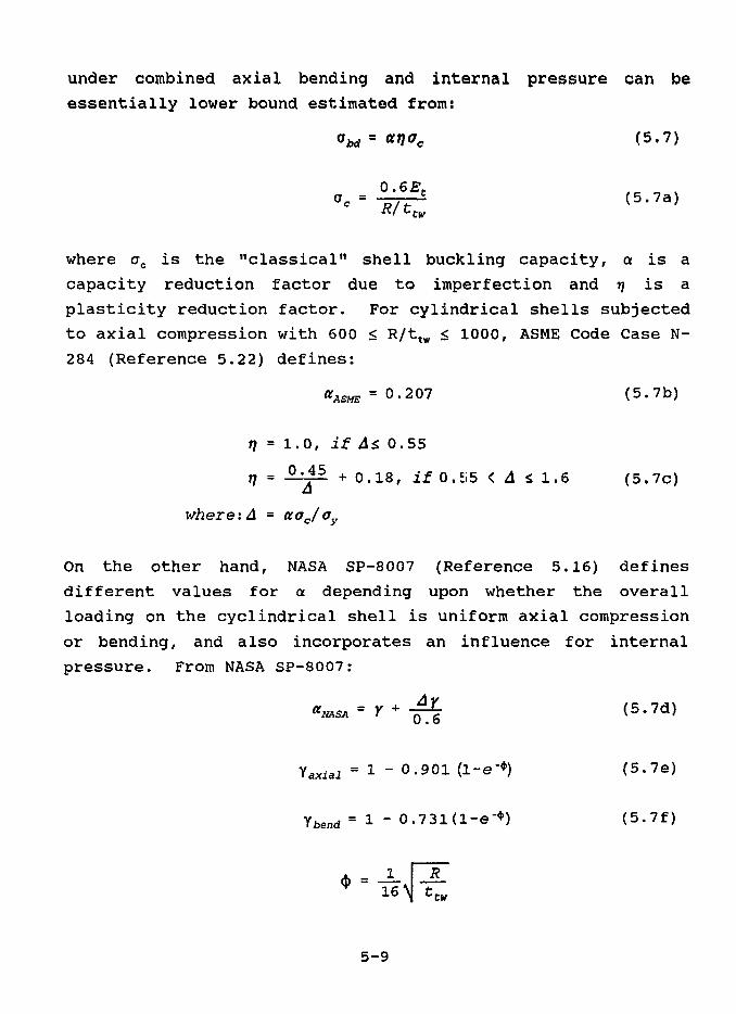
under combined axial bending and internal pressure can beessentially lower bound estimated from:

abd = «tjac (5.7)

°c = a/,.— (5.7a)

where crc is the "classical" shell buckling capacity, a is a

capacity reduction factor due to imperfection and rj is a

plasticity reduction factor. For cylindrical shells subjected

to axial compression with 600 < R/ttw < 1000, ASME Code Case N-

284 (Reference 5.22) defines:

= 0.207 (5.7b)

t] = 1.0, if A*. 0.55

r; = -2JJI + 0.18, if 0.55 < A £ 1.6 (5.7c)

where-. A = aajay

On the other hand, NASA SP-8007 (Reference 5.16) defines

different values for a depending upon whether the overall

loading on the cyclindrical shell is uniform axial compression

or bending, and also incorporates an influence for internal

pressure. From NASA SP-8007:

££ (5.7d)

axial = 1 " 0.901 (1-e-*) (S.7e)

1 " 0.731(l-e-*) (5.7f)

. _ 1 \ R

5-9

where A7 is an increase factor for internal pressure as given by

Figure 5.2 (Reference 5.16). In Figure 5.2, pan should be taken

as:

P«n = Pst + Pdh ~ 0.4pdv (5.7g)

which represents the minimum probabilistic combined pressure

against the tank side wall at the location of the maximum

longitudinal compressive stress and the time of occurrence of

the maximum moment.

In the judgment of the authors, the ASME Code Case N-284 value

for a (Equation 57b) is too conservative for bending-induced

axial stress which varies both circumferentially and

longitudinally, and also provides no credit for the beneficial

effect of internal pressure. However, the NASA SP-8007 value

for a (Equation 5.7d) is based on model tests which may not have

as severe of imperfections as actu?.l tanks, and may not be

adequately conservative. These issues are being further

investigated. In the meantime, for 200 £ (R/ttw) < -1500, it is

recommended that:

a = 0.8ccmsA £ 0.48 (5.8)

where 7 in Equation 5.7d is based on 7bend from Equation 5.7f.

The value of QtASME/7axial ranges% from 0.7 to 0.9 and averages 0.8

for (R/ttJ from 600 to 1000 where Equation 5.7b applies.

Therefore, the use of a factor of 0.8 in Equation 5.8 is

intended to provide about the same degree of conservatism for

the case of bending plus internal pressure as is contained in

Equation 5.7b for pure axial compression. The limit on a of

0.48 is intended to guard against excessively high values of a

due to the benefit of the internal pressure obtained from Figure

5.2.

The nominal buckling stress ab should be taken as the lesser of

abe (Equation 5.5), or abd (Equation 5.7). Then the maximum

5-10

permissible axial compression force per unit of circumferential

length is given by;

,5.9,where, FS = 1.34

In this equation, FS is the factor of safety required for ASME

Service Level D necessary to provide high confidence of avoiding

a buckling failure.

5.5 MOMENT CAPACITY AWAY FROM TANK BASE

At locations along the cylindrical shell away from the base, the

moment capacity is given by:

Mc = CbnR2 - ££ (5.10)

where Pa is any concurrent axial compressive force on the

cylindrical shell (generally negligible).

5.6 ANCHORAGE CAPACITY AT TANK BASE

The base anchorage bolt hold-down capacity, Tcb, is governed by

the weakest of the following elements:

1. Bolt tensile capacity

2. Anchorage of bolt into concrete foundation

3. Capacity of the top plate of bolt chairs to transfer bolt

loads to the vertical chair gussets

4. Attachment of the top plate and vertical chair gussets to

the tank wall.

5. Capability of tank wall to withstand concentrated loads

imposed on it by chairs

Each of these capacities should be based on code minimum

5-11

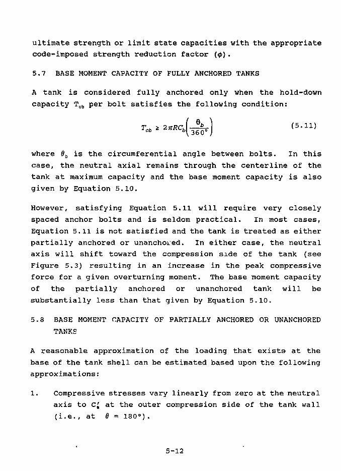
ultimate strength or limit state capacities with the appropriate

code-imposed strength reduction factor (<p) .

5.7 BASE MOMENT CAPACITY OF FULLY ANCHORED TANKS

A tank is considered fully anchored only when the hold-down

capacity Tcb per bolt satisfies the following condition:

where 8b is the circumferential angle between bolts. In this

case, the neutral axial remains through the centerline of the

tank at maximum capacity and the base moment capacity is also

given by Equation 5.10.

However, satisfying Equation 5.11 will require very closely

spaced anchor bolts and is seldom practical. In most cases,

Equation 5.11 is not satisfied and the tank is treated as either

partially anchored or unanchoired. In either case, the neutral

axis will shift toward the compression side of the tank (see

Figure 5.3) resulting in an increase in the peak compressive

force for a given overturning moment. The base moment capacity

of the partially anchored or unanchored tank will be

substantially less than that given by Equation 5.10.

5.8 BASE MOMENT CAPACITY OF PARTIALLY ANCHORED OR UNANCHORED

TANKS

A reasonable approximation of the loading that exists at the

base of the tank shell can be estimated based upon the following

approximations:

1. Compressive stresses vary linearly from zero at the neutral

axis to C£ at the outer compression side of the tank wall

(i.e., at 6 = 180°).

5-12

2. Uplift heights Sg vary linearly from zero at the neutral

axis to <S0 at the outer tension side of the tank wall (i.e. ,

at 0 = 0°).

3. For simplicity, fluid hold-down forces are also assumed to

vary linearly from Tfn at the neutral axis to Tf0 at 6 = 0.

Figure 5.3 illustrates the loading that exists at the base of

the tank wall based on the above approximation. Also shown is

the uplift of the tank wall due to an assumed rigid rotation of

the base. In Figure 5.3, C,' is the maximum compressive stress

in the tank wall, Tfn is the effective fluid hold-down force at

the neutral axis, ATf is the increase in fluid-hold down force

at $ - 0, Tbi are anchor bolt hold-down forces if the tank is

anchored, Wt is the tank weight, and Mc is the moment capacity

which results from this loading distribution.i

For any given angle 6n to the neutral axis:

n* Lbi

i = 1

2R

(5.12)

Mc = c'mCzR2 + £ (T^RcosB^ + TfnR

2(2sin6n) + ATeC4R2 (5.13)

where:

1 + cos 0n1 s i n On + (n-8n)cos 6A

r - s i n gncos dn * w - 6n2 1 + cos dn

(5.14)C 3 =

s in dn - 6n cos 6n

s in 6n + (jr-0n) cos 6n

1 + cos 6n-1 - cos 6.

r = gn ~ S i n 0n COS gn

'4 1 - COS 5n

5-13

Numberical values for C1f Ca, C3, and C4 as functions of 6n are

tabulated in Table 5.1.

The moment capacity depends upon the axial compressive buckling

capacity of the tank wall (Cb) from Section 5.4, the tensile

hold-down capacity of the anchor bolts including their anchorage

and attachment, to the tank (Tcb) from Section 5.6, the

permissible uplift height (£0) from Section 5.9, and the hold-

down force of fluid pressure acting on the tank base plate (Tf)

from Section 5.10. Thus, each of these quantities must be

estimated prior to estimating the overturning moment capacity.

The steps in solving for the moment capacity are as follows:

1. Establish the maximum permissible uplift height So (see

Section 5.9) .

2. Compute the fluid hold-down force Tf0 corresponding to the

uplift height 50 and the fluid hold-down force TTn at the

neutral axis (see Section 5.10) and then:

ATf=Tfo-Tfn (5.15)

3. Assume an initial value of the angle 0n to the neutral axis

and estimate the anchor bolt tension Tbl in anchor bolt "i"

from:

(Cos 6, - cos dn\

( i -cos g. Jr«*

where

and 9t is the angle 6 at bolt "i," Tbp is any bolt

pretension (generally should be taken as zero since it is

likely to be lost over time), Tcb is the bolt capacity (see

5-14

Section 5.6), Ab is the bolt area, Eb is the bolt modulus ofelasticity and h( is the effective bolt length from itsattachment to the tank to its effective anchor depth in theconcrete.

4. Compute C,' from Equation 5.12 and compare it to the shellbuckling capacity Cb. Vary 8n and repeat Steps 3 and 4until C/ = Cb.

5. Determine the moment capacity Mc from Equation 5.13.

As will .be shown in the solution for capacity of the exampletank in Appendix F, it is unnecessary to converge to a refinedestimate of the angle 0n to the neutral axis in Step 4 in orderto estimate the moment capacity Mc. Although C,' is sensitive tochanges in the angle 0n, Mc is not sensitive to small changes in

Also, as will be shown in Appendix F, the base moment capacityof even a minimally anchored tank is substantially greater thanthat of an unanchored tank. Therefore, for new designs it isrecommended that the tank should be. either laterally supportednear its top (thus greatly reducing the applied base moment) orshould be anchored at its base.

5.9 PERMISSIBLE UPLIFT DISPLACEMENT

In order to prevent anchorage failure, the maximum uplift

displacements So of anchored tanks should be limited to a small

value. For anchored tanks in which the bolt tensile capacity

controls Tcb, So should be limited as follows:

6O <; 0.01he (5.18)

where he is the effective bolt length. When other failure modescontrol, So should be limited to the lesser of Equation 5.18 or1/4 inch.

5-15

For unanchored tanks much greater uplift heights are

permissible. To avoid failure at the junction of the base plate

and wall, it is suggested that uplift heights be limited to:

60 = 0.1L (5.19)

where L is the computed uplift length of the base plate (see

Figure 5.5 and Section 5.10.2). Equation 5.19 will typically

produce uplift heights of several inches. However, if piping or

other components are attached to the tank wall or uplifted

region of the base plate, So must also be limited to tolerable

displacements for such piping or other components.

5.10 FLUID HOLD-DOWN FORCE

5.10.1 Anchored Tanks

Following the small displacement theory, the situation in the

region of axial tension in the tank wall is illustrated in

Figure 5.4 for a small uplift, S. At point "0" away from the

tank wall, the tank bottom is in full contact with the

foundation and the displacements, rotation, and moment in the

tank bottom are zero. However, at the intersection of the tank

bottom and wall at point "1," the tank bottom has uplifted 6 and

rotated a. The length of the uplift zone is L, and the fluid

pressure, pe, on the tank bottom and wall resists this uplift.

This uplift is accompanied by the development of tension, Tr, and

moment, Mf, in the tank wall at the intersection with the tank

bottom. This tension, Tf, acts as a fluid hold-down force on the

tank wall. For a given uplift height, 6, the hold-down tension,

Tf, that develops is both a function of the bending stiffness of

the tank wall which is a function of its thickness,. ttw, and

radius, R, and the bending stiffness of the base plate which is

a function of its thickness, ttb.

For a tank wall restrained against radial displacement at point

"1" by the base plate, the relationship between Mf and a can be

5-16

obtained from pages 276 through 278 of Flugge (Reference 5.18)

for axisyxnmetric loading as follows:

Mt = Ksa + Mfx (5.20)

where Mfx represents the fixed end moment, and

v - 2KK

J (5.20a)

E t3

12(l-v2t)

1 2

Even though the actual loading around the circumference is not

axisymmetic, Equation 5.20 is considered to be reasonably

appropriate for the actual loading condition.

Since L is a very small fraction of R, over the length L, the

base plate may be approximated as a radial beam. Thus, from the

boundary conditions at point "0":

b 2EtItb

S = PL* - MfL* (5.21)2AEtItb 6EtItb

where

Combining Equations (5.20) and (5.21), one obtains:

5-17

P*It (\ +24 \F)\l2EtItb p 6

(5.22)

k + (±)\ K*L2 «. j f e2 \ F}{ 12EtItb pL

(5.23)

(5.24)

P~e = " 8 " 2L2

(5.25)

where

F = 1 +

Using Equations 5.22 through 5.25, one can determine the uplift

height (<5) , tank wall hold-down tension (Tf) , and moment (Mf) ,

and maximum positive moment (M+) in the base plate as a function

of the uplift length, L, and fluid pressure, pe. From this

information the relationship between S and Tf is obtained. This

solution based on the small displacement theory is strictly

applicable under the following conditions:

1. (L/R) < 0.15. The solution ignores the stiffening of the

base plate from hoop behavior and thus conservatively

overpredicts the displacement S corresponding to a given Tfas!the ratio (L/R) becomes larger.

2. (5/ttb) < 0.6. This solution being based upon the small

displacement theory conservatively ignores the beneficial

effect that could be obtained by use of the large

displacement luembrane theory together with membrane

tensions in the base place to reduce S corresponding to a

5-18

given Tf. For unanchored tanks, it has been shown

(References 5.19 and 5.20) that the large displacement

membrane theory greatly increases the fluid hold-down

forces, Tf. Thus, for unanchored tanks, ignoring the large

displacement membrane theory is likely to lead to excessive

conservatism. For anchored tanks, the uplift heights (6)

are not expected to be so great and only moderate

conservatism is expected to result from ignoring large

displacement membrane effects. Unfortunately, no simple

solution exists for considering such membrane effects and,

therefore, currently one must either accept this source of

conservatism for anchored tanks or make judgmental

corrections to the computed fluid hold-down forces

following guidance from References 5.19 and 5.20.

3. (Mf/Mpb) < 0.9; (Mr/Mpw) < 0.9; and (M+/Mpb) < 0.9 where Mpband Mpw are the plastic moment capacity of the base plate

and tank wall, respectively. The previous solution is an

elastic solution and becomes nonconservative if these

conditions are not met. An alternate solution with plastic

hinges c*c locations where these conditions are not met is

easily formulated following the same approach as was used

herein but is judged to be unwarranted because violation of

these conditions is highly unlikely for S levels associated

with anchored tanks.

Only violation of the third condition leads to a nonconservative

estimate of the hold-down force Tf corresponding to a given

uplift displacement S. The first two conditions can be violated

so long as one is willing to accept the resulting conservative

underestimation of the fluid hold-down force.

For anchored tanks, it is recommended that the small

displacement theory be used to compute the fluid hold-down

forces. It is further recommendt<1 that the following pressures

5-19

be used to compute the fluid hold-down forces at locations 0 =

0 and 6 = 0n as defined in Figure 5.3:

Pe = Pst " Pdh ~ 0 • *Pdv at (5 = 0) (5 26)p e*p s t - O.ipdv at (d = dn)

(5*26)

The pressure defined at 6 = 0 represents the probable minimum

pressure at this location at the time the maximum moment occurs.

The pressure defined above at 0 = 0n represents the probable

minimum pressure at $ = 90° at the time the maximum moment

occurs, and is thus conservative for the location 6 = 8n since

6n will always exceed 90° for partially anchored or unanchored

tanks.

5.10.2 Unanchored Tanks

The small displacement theory of the previous subsection is

excessively conservative for unanchored tanks. An upper bound

theory is considered more appropriate and is used in the

following analyses.

The uplift length, L, illustrated in Figure 5.5, is assumed to

be a very small fraction of R, and, therefore, over the length

L, the base plate may be approximated as a radial beam. An

upper bound solution results after a full plastic hinge develops

at point "2" (location of maximum positive bending moment Mpb)

and at point "1" (base plate to wall junction and location of

maximum negative moment MpJ . Since no shear may cross point

"*,', the following relations hold:

£ £ l = [Mpb + Mpw] + Fh6 ( 5 -27)

and

Tf = poL (5 .28)

where Fh is the horizontal component of the membrane tension in

the base plate at its junction with the cylindrical shell.

5-20

Combining equations 5.27 and 5.28 one obtains:

Te = [2po [Mpb + Mpw + Fh6)f*

with

(5.29)

(5.30)

In Equation 5.29, Mpw is the smallest of the plastic moment

capacities of the following: (1) the base plate from Equation

5.30, (2) the tank wall with ttw substituted for ttb in Equation

5.30, and (3) the welded connection between the base plate and

wall. In Equation 5.30, aye should be as defined in Section 5.4.

An upper bound on the horizontal component of the membrane

tension in the base plate, Fh, is governed by the maximum local

hoop compression capacity of the tank wall. For an axisymmetric

application of Fh and Mpw at the base of the wall, the maximum

hoop compression in the tank wall occurs at the intersection of.

the wall and base plate and is given by:

= 2 * (5.31)

so long as

Conservatively NeB should be limited to (ayettw) . With this limit:

—f5 32}( 2 )

Local plastic hoop yielding might allow some increase in Fh but

it is recommended that no credit be taken for such an increase.

For conservatism, it is recommended that the probable minimum

pressure from Equation 5.26 be used for pft. Then Tfn is computed

5-21

from Equation 5.29 with S • 0, and TTo is computed with S » SQ.

The ATT is computed from equation 5.15.

5.11 BASE SHEAR CAPACITY

For large diameter (greater than about 30 feet) flat bottomtanks with fluid heights less than the diameter, it is commonand acceptable practice to rely on friction between the tankbottom and its foundation to provide the base shear capacity.Since the base shear response, Vr and the base overturning momentresponse, Mr are primarily due to the fluid horizontal impulsivemode of response, they both are maximum at the same time. Thus,the nominal sliding shear capacity is:

VCS=(COF) [Wa+ (jnrw)] (5.33)

where

(5.34)

STbl is the sum of anchor bolt tensions from the overturningmoment analysis, (COF) is the coefficient of friction betweenthe tank base and its foundation, pa is the probable averagefluid pressure on the base given by (pst — 0.4 Pdv) , and Wt is thetank wall and roof weight. The equivalent code capacity Vc isobtained by applying a strength reduction factor (</>) of 0.75 tothe nominal shear capacity Vcs, i.e.,:

Vc = 0.75Vcs (5.35)

Such a low factor (<£) is used because of the uncertainty

associated with the coefficient of friction.

For small diameter (less than about 10 feet) tanks, or tanks

with fluid heights substantially greater than the tank diameter,

it is unlikely that the friction-based shear capacity given by

Equation 5.35 will exceed the base shear demand from the DBE.

In this case, the shear capacity should be provided by anchor

bolts. It is not acceptable to credit friction for a portion of

5-22

the shear capacity and provide the remainder by anchor bolts.

Either 100% of the reported shear capacity is to be provided by

friction, or 100% must be provided by anchor bolts or other

means of positive anchorage.

Some large diameter flat bottomed tanks such as the example tank

have a slight cone to their bottom plate so that contained fluid

will always drain away from the center toward the drain pipe at

the edge. This cone is generally created by a variable

thickness sand cushion between the tank bottom plate and its

foundation. Furthermore, the tank bottom is generally made up

of slightly overlapped fillet welded individual plates. Thus,

the surface between the bottom plate and the sand cushion

contains a series of rough steps. Under these conditions, it is

reasonably conservative to estimate

(COF) > 0.7* (5.36)

For flat bottom steel tanks on concrete the COF is estimated as

0.55.

5.12 OTHER CAPACITY CHECKS

For tanks on soil sites, one should also check the capacity of

the tank foundation and this capacity sometimes governs.

Lastly, the possibility of piping failure or the failure of

nozzles/penetrations where such piping is attached to the tank

should be checked. Such failure will likely lead to loss of

tank contents. In fact, a significant fraction of the cases of

seismic induced loss of tank contents have been due to such

failures when the piping contained poor seismic details. The

issues to be checked are as follows:

1. Are heavy valves or long piping runs being supported

through the piping nozzles off either the tank walls or the

"Applicable for large diameter tanks with coned and uneven base.

5-23

bottom plate, or are they independently supported? If

heavy valves or long piping runs are being supported off

the tank, then the ability of the nozzles and the tank wall

or bottom plate to withstand the imposed seismic-induced

inertial forces should be checked. Methods outlined in

Welding Research Bulletin 107 (Reference 5.21) may be used

to compute local stresses in the tank wall, and the

strength acceptance criteria for vessels contained in

Chapter 3 can be used for the stress capacity.

2. Is there sufficient piping flexibility to accommodate

relative seismic anchor movements (SAM) between the

locations where the piping is supported from the tank wall

and where it is independently supported? Particularly for

unanchored tanks, the piping nozzle and tank shell should

be evaluated for their ability to withstand the expected

relative SAM.

5.13 TOP SUPPORTED TANKS

Many of the DOE underground waste storage tanks are laterally

supported by the surrounding concrete vault near the top of the

cyclindrical tank wall. As shown in Chapter 4, the presence of

this top lateral support will greatly reduce the overturning

moment applied at the base and will also reduce the base shear.

In this case, the base moment capacity (Section 5.8) and base

shear capacity (Section 5.11) are not likely to control the

seismic capability of such tanks, but should still be checked.

In addition, the lateral force (shear) capacity of the top

anchorage must be checked in accordance with the capacity

requirements of Section 3.7. Furthermore, these lateral forces

must be applied to the concrete vault when checking the seismic

capacity of the vault. Tanks with lateral support near the top

of the cyclindrical tank wall are likely to have substantially

greater seismic capacity than a similar tank without this top

support.

5-24

REFERENCES

5.1 Kennedy, R,P. and Kassawara, R.P., "Seismic Evaluation of

Large Flat-Bottomed Tanks", Second Symposium of Current

Issues Related to Nuclear Power Plant Structures,

Equipment, and Piping with Emphasis on Resolution of

Seismic Issues in Low-Seismicity Regions, EPRI NP-6437-D,

Electric Power Research Institute, May 1989.

5.2 "A Methodology for Assessment of Nuclear Power Plant

Seismic Margin," NP-6041, Rev. 1, Electric Power Research

Institute, June 1991.

5.3 Veletsos, A.S. and Yang, J.Y., "Dynamics of Fixed-Base

Liquid Storage Tanks," Presented at the U.S.-Japan Seminar

for Earthquake Engineering Research With Emphasis on

Lifeline Systems, Tokyo, Japan, pp. 314-341, November 1976.

5.4 Veletsos, A.S. and Yang, J.Y., "Earthquake Response of

Liquid Storage Tanks," Advances in Civil Engineering

Through Engineering Mechanics, Proceedings of the

Engineering Mechanics Division Specialty Conference, ASCE,

Raleigh, NC, pp. 1-24, 1977,

5.5 Veletsos, A.S., "Seismic Response and Design of Liquid

Storage Tanks," Guidelines for the Seismic Design of Oil

and Gas Pipeline Systems, ASCE, Chapter 7, 1984.

5.6 Veletsos, A.S. and Tang, Yu, "Interaction Effects in

Vertically Excited Steel Tanks", Dynamic Response of

Structures, ASCI, pp. 636-643, March 1986.

5.7 Veletsos, A.S. and Tang, Yu, "Dynamic of Vertically Excited

Liquid Storage Tanks," Journal of Structural Engineering,

Vol. 112, No. 6, ASCE, pp. 1228-1246, June 1986.

5-25

5.8 Haroun, M.A. and Housner, G.W., "Seismic Design of Liquid

Storage Tanks," Vol. 107, No. TCI, pp. 191-207, 1981.

5.9 Haroun, M.A. and Housner, G.W., "Complications in Free

Vibration Analysis of Tanks," Journal of the Engineering

Mechanics Division, Vol. 108, No. EM5, ASCE, pp. 801-818,

1982.

5.10 "ASCE Standard and Commentary—Seismic Analysis of Safety-

Related Nuclear Structures", ASCE 4-86, September 1986.

5.11 Newmark, N.M and Hall, W.J., "Development of Criteria for

Seismic Review of Selected Nuclear Power Plants", NUREG/CR-

0098, Nuclear Regulatory Commission, May 1978.

5.12 Priestly, M.J.N. et al., "Seismic Design of Storage Tanks,"

Bulletin of the New Zealand National Society for Earthquake

Engineering, Vol. 19, No. 4, December 1986.

5.13 Priestly, M.J.N., "Seismic Design of Storage Tanks,

Recommendations of a Study Group of the New Zealand

National Society for Earthquake Engineering", December

1986.

5.14 Rotter, J.M., "Local Inelastic Collapse of Pressurized Thin

Cylindrical Steel Shells Under Axial Compression", Research

Report, School of Civil and Mining Engineering, University

of Sydney, Australia, 1985.

5.15 "ASME Boiler & Pressure Vessel Code Section III",

Subsection NC3800, Division 1, 1989.

5.16 "Buckling of Thin-Walled Circular Cylinders", NASA SP-8007,

National Aeronautics and Space Administration, August 1968.


Construction, Load & Resistance Factor Design", LRFD, First

Ed., Chicago, Illinois, 1986

5-26

5.18 Flugge, W., "Stresses in Shells11, Springer-Verlag, 1960.

5.19 Manos, G.C., "Earthquake Tank-Wall Stability of Unanchored

Tanks," Journal of Structural Engineering, Vol. 112, No. 8,

ASCE, pp. 1863-1880, August 1986.

5.20 Haroun, M.A. and Badawi, H.S., "Nonlinear Axisymmetric

Uplift of Circular Lates," Dynamics of Structures, ASCE,

pp. 77-89, August 1987.

5.21 K.R. Wickman, Hooper, A.G. and Mershon, J.L., "Local

Stresses in Spherical and Cylindrical Shells due to

External Loadings," Welding Research Bulletin 107, August

1965.

5.22 Miller, CD., "Metal Containment Shell Buckling Design

Methods", ASME Code Case N-284, Rev. 1, May 1991.

5-27

NOTATION

Cb maximum permissible axial compressive force per unitlength

C , compressive force per unit length at the outercompression side of tank wall


hc height of cylindrical tank wall above the liquid

hd dome height above cylindrical wall

he effective length of anchor bolt

hsc slosh height capacity

hsr slosh height response

Itb moment of inertia of base plate

L length of uplifted portion of base plate


M moment in tank wall at intersection with base plate

M+ maximum positive moment

Mb base overturning moment response

Mc moment capacity of tank

Mf moment in tank due to fluid hold-down

MfX fixed end moment

Mpb plastic moment capacity of base plate

Mpw plastic moment capacity of wall

Nh horizontal component of membrane tension in base plate

Neil maximum hoop compression

p liquid pressure

pc pressure capacity

5-28

pdh hydrodynamic pressure due to horizontal component ofseismic motion

pdv hydrodynamic pressure due to vertical component ofseismic motion

pe effective pressure defined by Equation 5.26

p,n total minimum internal pressure on tank wall atlocation of maximum longitudinal compressive stress

pKX total maximum internal pressure on tank wall atlocation of maximum longitudinal compressive stress

pst hydrostatic pressure

pTl total inelastic factored demand pressure

Pa axial compressive force on tank wall

R radius of the tank

ttb thickness of base plate


Tbi tensile force on anchored bolt fti"

Tbp anchor bolt pretension

Tcb tensile capacity of anchor bolt

Tf( ) fluid hold-down tensile force (tension)

Tf0 fluid hold-down tensile force at the outer tensionside of the tank wall

Tfn fluid hold-down tensile force at the neutral axis

Vb base shear response

Vc base sliding shear capacity using code coefficient

Vcs nominal base sliding shear capacity

We effective weight for determination of base shearcapacity

Wt tank weight

6 uplift height at outer tension side of tank wall

5-29

<Se uplift height of tank wall at an angle 0


0b circumferential angle between anchor bolts

Bn circumferential angle to neutral axis

PX Poisson's ratio of tank material

ab governing axial stress capacity of tank wallconsidering buckling modes

abd axial stress capacity of tank wall in "diamond"buckling mode

abe axial stress capacity of tank wall in "elephant-foot"buckling mode

CT0 hoop membrane stress capacity

ay code minimum yield stress

aye effective yield stress

0 strength reduction factor

5-30

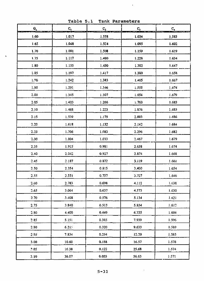
Table 5.1e, ! c,

1.60

1.65

1.70

1.75

1.80

1.85

1.90

1.95

2.00

2.05

2.10

2.15

2,20

2.25

2.30

2.35

2.40

2.45

2.50

2.55

2.60

2.65

2.70

2.75

2.80

2.85

2.90

2.95

3.00

?.O5

3.10

1.017

1.048

1.081

1.117

1.155

1.197

1.242

1.291

1.345

1.403

1.468

1.539

1.618

1.706

1.804

1.915

2.042

2.187

2.354

2.551

2.783

3.064

3.408

3.840

4.400

5.151

6.21.-'

7.834

10.60

16.38

36.07

Tankc2

1.558

1.534

1.508

1.480

1.450

1.417

1.383

1.346

1.307

1.266

1.223

1.179

1.132

1.083

1.033

0.981

0.927

0.872

0.815

0.757

0.698

0.637

0.576

0.513

0.449

0.385

0.320

0.254

0.188

0.122

0.055

Parametersc,

1.034

1.095

1.159

1.228

1.302

1.380

1.465

1.555

1.654

1.760

1.876

2.003

2.142

2.296

2.467

2.658

2.874

3.119

3.400

3.727

4.112

4.573

5.134

5.834

6.735

7.939

9.633

12.20

16.57

25.68

56.63

c«1.583

1.602

1.619

1.634

1.647

1.658

1.667

1.674

1.679

1.683

1.685

1,686

1.684

1,682

1.679

1.674

1.668

1.661

1.654

1.646

1.638

1.630

1.621

1.612

1.604

1.596

1.589

1.583

1.578

1.574

1.571

5-31

•CONCRETE MAT

Figure 5.1 Example Tank

5-32

Figure 5.2 Increase in Axial Compressive Buckling StressCoefficient of Cylinders Due to Internal Pressure(Reference 5.16)

5-33

N.A.

I COS g - l

V 1-C8 J C O S a - c o s e " )

V cosen /

M

Figure 5.3 V e r t i c a l Loading on Tank Wall a t Base

5 - 3 4

WALL

BOTTOM

I 1 I I i I t 1 I i I

M = 0

Figure 5.4 Schematic Illustration of Anchored Tank BottomBehavior at Tensile Region of Tank Wall

5-35

Pe

AT POINT 2

Figure 5.5 Schematic Illustration of Unanchored Tank BottomBehavior at Tensile Region of Tank Wall

5-36

CHAPTER 6

EVALUATION OF SOIL-VAULT INTERACTION

6.1 INTRODUCTION

This chapter contains provisions for evaluation of the seismic

motion input to the support points of the tank and the seismic

induced pressures acting on the walls of the vault. The first

result is to be used in the seismic evaluation of the tank

(Chapter 4), and the second result is to be used in the stress

analysis of the vault structure (Chapter 3) . The free field

criteria motion (defined in terms of a response spectrum) to be

used as input to this evaluation is discussed in Chapter 3. The

tank model used in the combined vault/tank system is discussed

in Chapter 4 and further amplified in this chapter.

There are two important considerations associated with an

evaluation of soil-vault interaction effects. The first

consideration relates to the evaluation of the vertical spatial

variation of the free field ground motion. A free-field motion

is defined at a control point and motions compatible with the

soil properties are computed at other locations in the free

field. This evaluation is performed using standard convolution

methods assuming vertically propagating, horizontally polarized

shear waves in the free field. The soil properties affecting

the vault response at many of the HLW sites are relatively

uniform over depths. At these sites it is reasonable to assume

that the free field motion is uniform with depth so that

convolution studies are not required to define the vertical

spatial variation of the ground motion.

The second consideration requires an evaluation of the

soil-vault interaction effects since the vault motion may differ

from the free field motion. Soil pressures acting on the vault

6-1

can be determined from this evaluation. There are two

approaches that have been used in the literature to evaluate

these effects. One approach is based on finite element models

of the free field and vault with continuity conditions at the

soil-vault interface used to connect the two models. A second

approach utilizes spring/damper models, connecting the vault

model to the free field, to represent soil-vault interaction

effects. Both approaches are recommended in References 6.1 and

6.2 and they have both been used extensively and successfully .in

seismic analyses of nuclear power plant facilities. The first

approach is theoretically rigorous and leads to excellent

results provided that the numerical details (element size,

frequency or time increments, and boundary conditions) are

properly treated. However, this approach is difficult and

costly to implement. The second approach is simpler and more

cost-effective, but the degree of its applicability to vaults of

the relatively small height-to-radius ratios encountered in HLW

storage facilities has not yet adequately been assessed.

Studies are currently underway to make this assessment and, if

necessary, improve the approach. Pending the outcome of these

studies, the simple approach may be used in the form described

herein, which is essentially the same as that given in

References 6.1 and 6.2.

An evaluation of the mass and stiffness characteristics of

typical vault-tank systems indicates that soil-vault interaction

effects are of minor significance for many vaults. Therefore,

the additional effort required to apply the first approach may

not be warranted for underground concrete vaults. Conditions

under whic"h the soil-vault interaction effects can be neglected

are also discussed in this chapter.

This chapter includes discussions of the definition of the

required soil properties, free field motion, response to

vertical seismic motions, response to horizontal seismic

6-2

motions, and vault-vault interaction effects. The provisions of

this chapter are applicable to vaults which are circular in

cross section. The results may be applied, however, to non-

circular cross sections provided that the longer plan dimension

is no larger than 1.5 times the shorter plan dimension. In

these cases the vault shall be assumed to be circular in cross

section with a plan area equal to the actual plan area.

6.2 SOIL PROPERTIES

Soil properties (shear modulus, density, Poisson's ratio and

damping) are required to perform both the free field convolution

studies and the soil-structure interaction (SSI) analyses.

These analyses should account for the dependence of these soil

properties on strain levels in the soil during the DBE.

Sufficient in-situ data should be obtained to find mean values

for the properties and to statistically define the variation of

the properties.

A soils exploration program should be implemented to evaluate

the soil properties to be used in the seismic analyses. The

exploration should be performed as close as practical to the

location of the tank and should extend down to a depth at least

equal to two vault radii below the vault foundation. Sufficient

data should be obtained so that variability in properties can be

statistically defined. The statistical evaluation of soil

properties should be done within layers which are. usually

defined from the boring logs. Information on properties of

backfill should be developed to the same degree as for the

in-situ soils. Details of the exploration program are discussed

further in Section 7.2.

Cyclic confined compression, resonant column or torsion testing

of undisturbed soil samples should be performed so that the

variation of soil properties (shear modulus and damping) with

strain levels may be defined. Soil damping should be limited to

6-3

15%.

As a minimum, SSI and convolution calculations should be

performed using 15 (lower bound), 50 (best estimate), and 85

(upper bound) percentile low strain soil shear moduli. These

convolution studies are not required if SSI effects can be

neglected by the criteria of Section 6.5.1. The lower bound

properties are equal to the best estimate divided by one plus

the coefficient of variation and the upper bound properties are

equal to the best estimate properties times one plus the

coefficient of variation. The minimum coefficient of variation

should be taken as 0.5. If sufficient soil data is not

available to evaluate the standard deviation of the shear

modulus, the coefficient of variation should be taken as 1. The

soil damping should be selected consistent with the strain

values determined from the convolution analyses.

6.3 FREE FIELD MOTION

The objective of the calculations discussed in this section is

to determine the variation of the two horizontal components of

the free field ground motion over the depth of embedment of the

vault. This variation should be included in the SSI

calculations used to evaluate the seismic-induced motion of the

tank and the soil pressures acting on the vault during a seismic

event. If a site-specific study has been performed, these data

will be available. In the case that the site is uniform (see

Section 3.3), the DBE horizontal ground motion can be

conservatively assumed to be uniform over the depth of the

vault. Convolution studies are still required, however, to

evaluate the magnitude of the seismic-induced soil strains which

are required to determine the strain-dependent soil properties

to be used in the SSI analyses. The vertical component of the

free field motion can be taken as the criteria motion specified

at the basemat of the vault (see Section 6.4).

6-4

A DBE time history should be developed which results in response

spectra that envelope the free field spectra discussed in

Chapter 3. Response spectra should be developed for the time

history at all damping values of interest and these spectra

should be compared with the free field criteria spectra

discussed in Chapter 3. Criteria specified in ASCE 4-86

(Reference 6.1) can be used for this comparison. Special care

should be taken so that the time history is base]ine corrected

(i.e., final velocity of the time history is zero and peak

displacements are consistent with the magnitude and focal

distance of the DBE).

The control point for the placement of the DBE horizontal ground

motion should be taken as discussed in Section 3.3. The

variation of horizontal free field motions occurring at

elevations within the depth of the vault should be evaluated

using convolution methods associated with vertically

propagating, horizontally polarized shear waves. The number and

thickness of the layers to be used in the analysis should be

consistent with the soil property variation with depth. The

mesh size shall be sufficiently fine over the depth of the vault

to provide ground motion data at the top midpoint and bottom of

the vault, and be capable of transmitting frequencies containing

most of the energy in the DBE and at least twice the primary

system frequencies (e.g., SSI, fixed base structural, and

equipment) . However, the mesh does not have to transmit

frequencies greater than 25 cps. Larger mesh sizes r.sy be used

if justified with a parametric study. Convolution studies

should be performed using lower bound, best estimate, and upper

bound soil properties. The free field motion using the three

soil models shall be used as input to the SSI calculations for

the corresponding soil models.

The convolution calculations should be performed accounting for

the degradation of soil properties (shear modulus and hysteretic

6-5

soil damping) with strain. The degradation models should be

determined from measured properties or computed using generally

accepted models. In no case should hysteretic soil damping be

taken as greater than 15%.

The convolution studies should be performed using in-situ soil

properties unless backfill has been used and the backfill

extends out an average distance of at least 3 vault radii from

the vault wall. In this case, the backfill properties should Jbe

used in the convolution analysis for the upper portion of the

soil column.

6.4 VERTICAL SSI CALCULATIONS

Vertical SSI parameters are given in Appendix G and used to

evaluate the significance of vertical SSI effects. The vertical

SSI damping ratio (fv) as determined in Section G.3 is given by:

C = 0. 59 [Rvpfs/ (HvPv) ]^2 (6.2)

where,

Rv = radius of vault

Hv = height of vault

pfs = mass density of foundation (base) soil

pv = average mass density of vault/tank/contents (total

mass/volume)

Most of the tanks of interest have aspect ratios (Rv/Hv) close to

unity so that the vertical SSI damping ratios are about 60% of

critical when the mass density of the vault tank system is about

equal to the soil (a reasonable assumption for most vaults of

interest) . This damping will eliminate any significant

amplification of the free field vertical motion (an

amplification of about 5% of the free field vertical motion

would be expected at the vertical SSI frequency). The vertical

motion of the tank can therefore be taken as equal to the free

field vertical motion described with the response spectrum as

6-6

given in Chapter 3.

The vertical seismic load on the roof of the vault can be

computed as the mass of the vault roof and overburden soil times

an acceleration taken from the spectrum defined in Chapter 3.

The acceleration should be taken from the spectrum at the

vertical fixed-base frequency of the vault including the mass of

the overburden soil and the flexibility of the roof of the

vault. Vertical SSI calculations can be performed using either

lumped parameter or finite element models. In either case, the

vault model should include the mass of the overburden soil and

the flexibility of the vault roof and walls. The fluid tank

model should represent the masses and frequencies discussed in

Section 4.5. The SSI model used for the lumped parameter

analysis can be taken from Section G.3.

6.5 HORIZONTAL SSI CALCULATIONS

Methods for calculation of the combined horizontal and rocking

seismic response of the vault/tank system are discussed in this

section. The cases in which the horizontal/rocking SSI effects

may be neglected are first discussed and this is followed by

consideration of the methods that may be used to include these

SSI effects when required.

6.5.1 Conditions for Neglecting Horizontal/Rocking SSI Effects

Horizontal and rocking SSI effects may be neglected when the°

site is relatively uniform (see Section 3.3 for definition of a

uniform site) and when it can be shown that the amplifications

of the free field motions caused by SSI effects are small. When

this is the case, the vault seismic motion can be taken as

uniform over the depth of the vault and expressed by the free

field spectra as defined in Chapter 3.

The horizontal and rocking SSI frequencies and damping ratios

are given in Appendix G. Amplifications of the free-field

6-7

motion caused by the SSI effects are calculated and shown in

Figure G.2 for various ratios of the vault height to the radius

(Hv/Rv) . These data indicate that coupled horizontal/rocking SSI

effects can be neglected for values of Hv/Rv less than 0.5 and

should be included for larger values of Hv/Rv.

When the SSI effects are neglected, the normal horizontal soil

pressure (p) acting on the vault can be uniformly distributed in

the vertical direction and distributed (in a cosine variation)

around the circumference of the vault. The magnitude of the

peak pressure can be conservatively (since it neglects the

contribution of shear forces acting on the vault wall) estimated

based on the peak inertial force required to act on the vault

wall so that the vault follows the free field motion. The

result of this assumption is:

p = YvRvamax cosB (6.3)

where,

7V = average density of vault/tank system


0 = angle defining location of point on perimeter of vaulta«ax = Peak free field acceleration (G's)

These wall pressures are in dynamic equilibrium with the

inertial loads acting on the tank/vault system. Since the major

portion of the inertial loads arises in the tank, the earth

pressures on the vault wall are in equilibrium with the inertial

loads in the tank. The stress analysis of the vault can

therefore be performed by placing the earth pressures on the

vault while supporting the vault in a manner that is compatible

with the support conditions for the tank within the vault. The

vault should be supported as a cantilever off the base and

subjected to the earth pressures when the tank is supported only

from the base of the vault. The vault should be treated as a

6-8

simple beam, supported at the top and base when the tank is top-

supported .

6.5.2 Criteria for Performing Horizontal SSI Calculations

This section covers the procedures that can be used when it is

required to include horizontal/rocking SSI effects, It should

be emphasized that the required outputs from these analyses are

response spectra at various locations within the vault/tank

system and soil pressures acting on the vault walls. A detailed

stress analysis of the vault and tank may subsequently be

performed using equivalent static loads developed from the

spectra and pressures determined from the SSI analyses.

Alternately, internal forces in the vault structure may be

determined directly from the SSI analyses provided the vault is

modeled in sufficient detail. In general, the tank forces

should be developed from separate analyses as discussed in

Chapter 4 of this report. The tank analyses would use either

the time histories or response spectra resulting from the SSI

analyses.

The treatment of SSI effects for the waste tanks is different

from the treatment of these effects for other structures such as

reactor containment buildings. The geometry, mass, and

stiffness of waste tanks cause vault wall SSI effects to be

larger than base SSI effects. The opposite is true for most

structures located at nuclear power plant facilities. This

difference is significant because there are fewer uncertainties

for base SSI models than for vault wall SSI models. A second

difference arises because of the significance of the soil

pressures exerted on the vault walls as a result of the seismic

loading. The standard SSI methods are modified so that these

pressures can be obtained. Both these differences require more

accurate vault wall SSI models than are usually needed for

evaluation of nuclear facilities. Currently, studies are

underway to refine the methods discussed in this chapter and the

6-9

results of these studies will be incorporated into this report

as they become available.

Two methods are available for performing the SSI calculations.

The first utilizes spring/damper lumped parameter models

connecting the vault and free field models to represent SSI

effects. In the second method, the soil and vault are

represented by a continuum modeled with discrete elements (e.g.,

finite elements) and the SSI effects are obtained based on

compatibility conditions at the interface. In either of these

cases the solutions may be carried out in the frequency or time

domain. The discretization parameters (e.g., time or frequency

increment, element size, boundary locations, etc.) should be

selected based on the desired frequency content of the solution.

Criteria such as those contained in the US NRC Standard Review

Plan (Reference 6.2) or in ASCE 4-86 (Reference 6.1) may be used

to satisfy these requirements. Solutions to the spring/damper

lumped parameter model may be obtained by using either a time

history analysis or a response spectrum analysis... Both are

discussed in the following sections. The response spectrum

solution should be restricted to those cases where the soil

conditions are uniform (see Section 3.3).

6.5.2.1 Lumped Parameter Model Using Time History Analysis

SSI calculations may be performed using a lumped parameter

spring/dashpot model to represent the connection of the

vault/tank to the free field.

Specification of Free Field Motion

At uniform sites (see Section 3.3) the horizontal component of

the free field motion may be taken as uniform and equal to the

DBE motion discussed in Chapter 3. At nonuniform sites the

horizontal component of the free field motion should be

specified at the top, bottom, and several intermediate depths

6-10

over the tank. These motions should be compatible with the DBE

free field motion (see Chapter 3) and the soil properties, and

should be generated based on convolution methods as discussed

above (Section 6.3). The sloshing motion of fluid and the

relative displacement component of the seismic-induced pressure

acting on the vault depend on the low frequency content of the

free field motion. The time history generated to fit the

criteria DBE spectra will often contain excessive low frequency

energy content unless care is taken in fitting the spectra with

the generated time history. This could result in over-

conservative predictions for sloshing motion and vault pressure.

Vault Model

The mass and stiffness characteristics of the vault should be

modeled. The stiffness properties of the vault should be

consistent with the current materials conditions and should

include any degradation of the structure which may have occurred

or will occur at the end of its service life. If uncertainties

exist regarding the current material conditions, suitable

variations in the model should be included in the analyses. The

vault may be assumed to be rigid if the fundamental fixed base

frequency of the vault is at least twice the SSI frequencies or

greater than 33 cps. In general, the SSI analyses will be used

to evaluate pressures acting on the vault structure. A separate

pseudo-static analysis will be used to evaluate stresses in the

vault.

Tank and Contents Model

The fluid/tank model to be used in the SSI analyses should

properly account for the fluid impulsive vibration mode and may

include the first convective mode of the fluid. The model

characteristics may be taken directly f -om the results given in

Chapter 4. The model is shown on Figure 4.6 and discussed in

Section 4.3.9.

6-11

The accelerations (e.g., At and Ae1 of Equation 4.32) of Chapter

4 used to find tank loads (moments and shears) and slosh heights

are the accelerations of the masses (which are evaluated during

the SSI calculation) of the tank model shown on Figure 4.6.

These may be used directly to perform stress analysis of the

tank.

It should be noted that the tank model results in the proper

total overturning moment and horizontal load applied to the

vault by the inertial loads of the tank and its contents.

Except for the cantilever tank, however, it does not provide the

distribution of these loads to the points at which the tank is

supported from the vault. This distribution must be done before

the stress analysis of the vault can be performed. The detail

methodology to be used in distributing the loads is discussed in

Section 4.3.7.

Soil Model

Results should be obtained for the best estimate, lower bound,

and upper bound soil models with the variations taken to be the

same as discussed in Section 6.2. The soil properties should be

compatible with soil strains as determined from the soil column

convolution studies.

Lumped Parameter SSI Coefficients

The lumped parameter SSI spring/damper models should be divided

.into those located at the foundation of the vault and those

along the side soil. Generally accepted solutions for these

parameters exist and may be used for these analyses. The free

field input to these models should reflect the variation in the

horizontal ground motion over the depth of the tank. Backfill

properties should be used to compute the side soil parameters.

When large differences exist between the backfill and in-situ

soil properties, Reference 6.3 may be used to obtain the side

6-12

soil interaction parameters.

An acceptable foundation spring/damper model for circular cross

section vaults is given in Appendix G. This spring/damper model

may be used for "near square" (where the long plan dimension is

less than 1.5 times the short dimension), hexagonal, octogonal,

and similar vault cross sections based on equivalent areas.

Alternate models are required for other shapes. The side soil

spring/damper model may be uniformly distributed over the depth

of the vault using the following spring/damper moduli:

Side Soil Spring Modulus = kss = 4.05 Gss (6.3)

Side Soil Damper Modulus = css = 9.90 Rv (pss Gss)1/2

where,

Gss = Shear modulus of soil along side soil

pss = Mass density of soil along side soil

Rv = Vault radius

kss = side soil SSI spring modulus

css = side soil SSI damper modulus

Calculation of Wall Pressures

The pressures acting on the vault wall should be determined from

the side soil forces computed from the relative motion of the

vault and free field. For vaults with a circular cross section

it may be assumed that the wall shear pressures are zero and

that the normal pressures are distributed in a cosine variation

around the circumference of the vault. The resulting pressure

distribution is:

pn = f cos0 / (n R) (6.4)

where,

pn = normal pressure

f = sidewall force at elevation of interest

0 = angle defining circumferential location on tank

Wall pressures for vaults of other shapes should be determined

6-13

in a manner consistent with the spring/damper models used for

these geometries.

Maximum Pressure Cutoffs

The response solutions may be developed based on the assumption

that nonlinear effects are unimportant so that the SSI

spring/damper models have constant values. The wall pressures

developed from these solutions may, however, be limited -by

Coulomb-Mohr soil strength parameters. When this is done the

ductility factors used for the stress analysis of the vault (see

Chapter 3) should be limited to unity. The computed peak

pressures may be reduced based on the Coulomb-Monr strength

parameters. The peak normal pressures may be limited by:

pc = av [tan2 (45 + 0/2) - 1/2] + 2 C tan (45 + 0/2) (6.5)

pt= CTV [tan2 (45 - 0/2) - 1/2] - 2 C tan (45 - 0/2)

where,

C = cohesive strength of soil

pc = peak compressive pressure in excess of at rest static

pressure

pt = peak tensile pressure below static pressure

av = vertical normal stress in soil at depth of interest

0 = angle of internal friction in backfill soil

Combination of Three Dimensional Input

SSI solutions should be carried out for the seismic input in

each of the three directions (two horizontal and vertical). The

total seismic response of the vault/tank system can be computed

by either SRSS of the responses computed in each of the three

directions or by absolute sum of the responses in e,.ch of the

three directions. In the latter case 100% of the largest

response shall be combined with 40% of the response in each of

the remaining two directions.

6-14

Generation of Response Spectra

Response spectra should be generated at locations of interest

using the criteria as specified in Reference 6.2.

6.5.2.2 Continuum Model Using Time History Analysis

As an alternative to the lumped parameter method described

above, the SSI calculations may be based on a continuum model of

the vault/tank/soil system. Since the computer codes used to

implement these solutions are usually quite complex, special

care should be taken to ensure that the code being used has been

verified. The following procedures of Section 6.5.2.1 also

apply to this Section: Specification of Free Field Motion, Vault

Model, Soil Model, Maximum Pressure Cutoffs, and Generation of

Response spectra.

Mesh (Element and Total size) Requirements

The mesh size and placement of boundaries should be consistent

with the required frequency content of the solution. Criteria

for these data may be taken from References 6.1 or 6.2.

Tank and Contents Model

The cantilever model of the tank and its contents, discussed in

Section 4.3.9, results in the proper total overturning moment

and total horizontal load applied to the vault by the tank

during the seismic response. It does not, however, distribute

these loads to the tank support points on the vault for the top

supported tanks. A modification is required to the model of

Section 4.3.9 if this load distribution is to be used in the

solution. This modification is required for most computer codes

used to implement continuum solutions since the same model of

the tank is used to compute the seismic response of the

vault/tank system and the stresses in the vault. The

computation of stresses in the vault, of course, requires that

6-15

the tank loads are properly distributed on the vault.

A general model that can be used to represent tne tank inevaluating the combined horizontal and rocking seismic responseof the tank/vault system is shown on Figure 6.1. The modelconsists of two cantilevers, one supported from the vault at theelevation of the top tank support and the other at the base ofthe tank. A rotary inertia must be added at the base for theimpulsive mode. The magnitude of the rotary inertia is given oncolumn 6 of Table 4.2. This model applies to all supportconditions and reduces to the model of Section 4.3.9 for thecantilever support condition.

In general two mass models are used: one representing theeffects of the impulsive fluid mass and the other representingthe response of the convective fluid mass. While the effects ofthe convective mass may not be significant, inclusion of thismodel allows one to determine the sloshing height of the fluiddirectly from the seismic response computation. The symbolsshown on Figure 6.1 apply to either the impulsive or convectivemode and the differences between the two modes are introducedwhen the parameters are numerically defined. The parameters ofthe model are given for the full tank which represents the mostsevere load case. Solutions are not available as yet forpartially filled tanks which have top supports.

The distribution of fluid mass (m£) between the impulsive (it )

and first convective mode (mc1) are given in columns 3 and 7 of

Table 4.2 respectively. The distribution of mass between the

top and base cantilevers is proportioned to achieve the proper

force distribution between the two supports so that:

mt = (l-mb/m*)m* (6'6)

6-16

where,

rob/in* = 1 for cantilever tanks in either impulsive or

convective mode

=0.6 impulsive mode for roller or hinged upper support

= ac1 (Table 4.4) for convective mode top-supported tank

m* = n or mc1 for impulsive and convective modes,

respectively

The lengths of the cantilever beams in the model are determined

to match the top and base support moments. These moments

consist of components due to the fluid pressure acting on the

basemat and fluid pressure acting on the tank wall. The

resulting cantilever heights are:

h'b = [d(0)+e] (mt/m*)Ht/(mb/m*) (6.7)

h't = d(l) (mt/m*)Ht/ {l-mb/w*)

where,

d = moment coefficients to account for fluid pressure

acting on the tank wall and defined in Tables 4.5

through 4.10. These coefficients depend on the tank

support condition and whether the mode is impulsive or

convective. Note that d(0) and d(l) define the moment

coefficients at the lower and upper supports,

respectively•

e = moment coefficients to account for fluid pressure

acting on basemat and defined in columns 4 and 11 of

Table 4.2 for the impulsive and convective modes,

respectively.

Ht = height of tank

Note that negative values of hj or h( indicate that the

cantilever extends below the support rather than above.

6-1?

The correct seismic acceleration imposed on the masses of themodel is obtained by matching the frequencies of the cantileverbeams to the tank frequency (fo1 or ft) as given in Sections4.3.2.1 (convective) and 4.3.2.2 (impulsive) respectively. Thisis done by selecting the stiffness of the cantilever beam (El)as:

[El] = 4,n2f*L3m/3 (6.8)

where,[El] = top or bottom cantilever stiffness for either

impulsive or convective modef = either fo1 or fi for convective or impulsive mode

respectivelyL = hj or h{ for the base and top cantilever models

respectivelym = top or base mass associated with the mode being

considered (convective or impulsive)

If the length of the top cantilever is zero, the -mass must be

attached to the support with a spring of rate (kc) so that the

tank frequency is matched. This spring rate will be:

kc = 4n2f2rn*(l-mb/m*) (6.9)

The accelerations (e.g., AJ shown in Chapter 4 and used to

determine bending moments in the tank and fluid slosh heights

can be related to computed accelerations of the top (At) and base

(Ab) masses of the model by:

A^+GVAt,) {z*-h'b)/{Ht+h't-h'b) (6.10)

where,

z* = center of gravity of the two masses

= [mt<Ht+ht')+mbh'b]/(mt+mbn

As an alternate to this model, i t is possible to include a

detailed model (e.g., finite element model) of the tank and

6-18

fluid in the soil/vault model. As discussed in Section 4.1, the

validity of these models should be estab.tished by comparing the

results for limiting cases obtained using the detailed model

with results obtained using the methods discussed in Chapter 4.


Many of the available computer codes do not have the option of

directly providing pressures acting on the vault walls. Such

pressure data are useful in verifying the results of the

computer solutions. Post processors should be developed so that

the output of these codes can be used to obtain wall pressures

at a time when vault member loads are close to the maximum.

6.5.2.3 Lumped Parameter Model Using a Response Spectrum

Analysis

A responss spectrum analysis may be performed for those vaults

founded in a uniform soil medium. This «iei.f .-ct is likely to be

over-conservative since phasing between the response modes is

lost in the calculations and they are therefore combined in a

conservative manner. This method of analysis may be used to

determine soil pressures acting on the vault and forces acting

on the tank. Direct spectra generation techniques may be used

to determine floor response spectra within the vault/tank

system. The following specifications of Section 6.5.2.1 also

apply to this Section: Specification of Free Field Motion, Vault

Model, Tank and contents Model, Soil Model, SSI Model, and

Maximum Pressure cutoffs.

The response spectrum analysis may be applied to a model of the

soil/vault/tank system satisfying the above criteria. This

analysis involves: computing the modes of the system (frequency,

mode shape, modal mass, modal damping, and modal participation

factor) ; evaluating the peak response for each of the modes; and

combining the modal responses. Mode combinations should be in

6-19

accordance with the procedures described in Reference 6.1.


The response spectrum analysis will provide peak relative

displacements and velocities between points on the vault and the

free field. The peak pressures may then be obtained by

multiplying these values by the side soil stiffness (kss) and

damping moduli (css) respectively and summing the results.

6.6 VAULT-VAULT INTERACTION

There is some evidence indicating that vault-vault interaction

effects are not significant unless the spacing between vaults is

less than one half vault radii. Additional studies are underway

to confirm these conclusions and to develop definitive guidance

in this area. Until such data become available, vault-vault

interaction effects should be evaluated for spacings closer than

one half of the vault radius.

6-20

REFERENCES

6.1 ASCE 4-86, "Seismic Analysis of Safety Related Nuclear

Structures," September 1986.

6.2 "U.S. NRC Standard Review Plan", NUREG-0800.

6.3 Veletsos, A.S. and Dotson, K.W., "Horizontal Impedances

for Radially Inhomogeneous Viscoelastic Soil Layers",

Earthquake Engineering and Structural Dynamics, Vol.16,

1988.

6-21

NOTATION

A,,ax peak free-field accleration

cw vault wal.l damper modulus

cBS side soil damper modulus per unit depth

DBE design basis earthquake

(EI)b stiffness of base cantilever model for tank and content

(EI)t stiffness of top cantilever model for tank and contents

g acceleration due to gravity

Gfs shear modulus of foundation soil

Gss shear modulus of soil along wall

h'b length of base cantilever model for tank and contents

h't length of top cantilever model for tank and contents

Hv height of vault

kss side soild spring modulus per unit depth

kw vault wall spring modulus

mb mass of base cantilever model for tank and contents

mt mass of top cantilever model for tank and contents

ps normal horizontal soil pressure on the vault wall

psc peak compressive soil pressure

pst peak tensile soil pressure

SSI soil structure interaction

Rv radius of vault

7 average weight density of vault-tank system

fv vertical SSI damping ratio

6 circumferential angle defining location on the vault

pfs mass density of foundation soil

6-22

ps, mass density of soil along vault wall

pv average mass density of vault, tank and contents

ffsv vertical intergranular stress in soil

0 angle of internal friction in backfill soil

6-23

•• *.'••'• >••'.'•'•*• /••"/•*•'.••'•* >*.*/•• V;*.' :"'."£&)'

Top Support

TH,

I

Tank Vault System

Alternate Model ifh', or hj = 0

T1

" i b l

Tank Model

h; (ED,Vault Model

hCantilevers Concentnc With

Vault Model. Offset forIllustration Only

Figure 6.1 Model for Tank-Fluid System

6-24

CHAPTER 7

CRITERIA FOR UNDERGROUND PIPING

7.1 INTRODUCTION

The acceptable design of underground piping must demonstrate

analytically the ability of the piping to withstand any strains

and stresses caused by potential seismic movement of foundation

soils in conjunction with those stresses induced by other normal

or accidental loadings applied to the piping. Stress resultants

(forces and moments) computed from these various load conditions

must be suitably combined to obtain stresses and strains which

can be shown to be less than the appropriate allowables.

Unfortunately, current Codes typically used for piping systems

do not specifically mention design requirements for underground

piping systems. Recommendations for such design criteria are

included in this document. The references listed at the end of

this document can be used to address specific issues of the

analysis problem. Specifically, design recommendations

appropriate for steel piping were obtained from Reference 7.23.

Potential seismic effects on underground facilities are, in

general, caused by different aspects of ground movements,

namely, (1) abrupt relative displacements of the ground caused

by dislocation at the ground surface from fault dislocations,

(2) ground failure of relatively large areas caused by

liquefaction, landslides, gross surface settlements, or collapse

of voids at depth, (3) transient deformation of the ground

during the seismic event due to wave passage effects, and (4)

transient movements of anchor points or buildings connected to

the underground facilities. For construction of new facilities,

zones susceptible to abrupt ground movements or ground failure

should be avoided. However, for evaluation of existing

facilities, the effects of these potential seismically induced

movements must be suitably accounted for and incorporated into

7-1

the evaluation. As described in Reference 7.9, rigorous

analytic treatment of the response of underground facilities to

these movements is in general not practical, particularly for

the case of transient effects. Therefore, conservative

procedures must be adopted to ensure that stresses and strains

remain within the recommended design allowables.

7.2 REQUIRED SEISMIC AND SOIL DATA

Appropriate seismic and soils data must be assembled to allow

for evaluation of the maximum responses and loadings of * the

underground facilities. The seismic environment must include

estimates of peak ground acceleration (PGA), peak ground

velocity (PGV), and peak ground displacement (PGD) defined at

the ground surface appropriate for the hazard specification.

Details on recommended procedures to be used to define the

seismic environment at a particular site are presented in

Section 3. If site specific evaluations are not available, but

broad banded ground response spectra anchored to PGA are used,

estimates of the PGV and PGD must be estimated from other

appropriate approximations. For a particular site, the approach

used to estimate these parameters must be justified.

Sufficient data should be gathered to suitably identify the

foundation soils surrounding the underground components and

determine their appropriate parameters. These can be gathered

using standard methods of foundation investigation, namely,

standard borings taking standard penetration test (SPT) drive

samples, cone penetrometer testing, seismic reflection surveys,

crosshole, uphole and/or downhole geophysical testing, etc. Of

specific interest for the program is to ascertain soils

susceptible to liquefaction, densification leading to ground

settlement, ground collapse at depth or near surface landslides.

The investigators should be aware of the guidance provided in

two publications of the Nuclear Regulatory Commission, namely,

Regulatory Guides 1.132 and 1.138, (References 7.12 and 7.13)

7-2

which present recommendations for geotechnical investigations

and laboratory testing. Such investigations must also suitably

define changes of soil properties along the route of the

underground facilities.

Soil properties of specific interest include:

• grain size distribution description

• plasticity characteristics

• density and relative density

• equivalent SPT blow count information

• effective coefficient of subgrade reaction

• liquefaction potential

• equivalent cyclic properties obtained from either site

specific laboratory testing or generic data for

appropriate soil types.

Enough data must be available to allow for evaluation of the

effect of seismically induced pore pressures on ground movements

and the loads induced on the underground system from relative

movements between the ground and the piping.

7.3 ANALYSIS LOADS AND CONDITIONS

When either analyzing or designing underground pipinc* to

withstand seismic effects, only those loadings which can

normally be expected to occur during the event need be

considered. The following load conditions should be considered

where appropriate:

1. Internal pressures developed during normal operation or

from accidental conditions.

2. External pressures caused by overburden soils and other

surcharge loadings. The type of underground pipe, method

of installation and bedding characteristics should all be

accounted for when determining the effects of these

7-3

external loads (Reference 7.15).

3. Thermal variations to which the piping will be subjected.

4. Permanent vertical settlements (total and differential) due

to densification of dry or partially saturated soil from

ground shaking or post-earthquake dissipation of pore

pressures developed in partially saturated or saturated

soils as well as settlements of soft zones or voids at

depth due to reconsolidation or collapse.

5. Development of liquefaction conditions in soils immediately

surrounding or below the underground pipe which may lead to

permanent vertical and horizontal movements from ground

failure. Possibility of flotation of underground

facilities with average densities less than that of the

surrounding soils must also be considered.

6. Alignment of the buried facility may extend through or

adjacent to areas where slopes exist. The stability of

these slopes must be assured for both normal operating

conditions as well as the design seismic event including

the potential effects of pore pressure development.

Potential disruption of underground piping from ground

failure due to slope instability and lateral spreading

effects must be considered.

7. Transient differential movements due to passage of seismic

ground waves as well as seismic movements of buildings and

other attachment points.

If unacceptable conditions are found to develop from any of the

conditions listed above, namely, from transient wave passage

effects, permanent ground settlement and/or ground failure

phenomena, alternate solutions must be developed to preclude

failure of the underground piping, particularly for safety class

piping, This approach must be followed for either new or

7-4

existing facilities. Such procedures can include rerouting the

piping, removal and replacement of poor soil surrounding the

underground piping, application of soil stabilization procedures

(e.g., grouting, densification, slop stabilization, permanent

dewatering of affected areas), or supporting the underground

piping on alternate supports such as pile supported cradles.

7.4 ANALYSIS PROCEDURES

Due to the complexity of the seismic problem as well as

difficulty in assessing controlling properties of foundation

soils, it is recommended that conservative methods of analysis

be used to estimate stresses and strains developed by each load

component and condition. Suitable variation in soil properties

must be included in these evaluations to account for the normal

variability in soil properties. In addition, the

recommendations presented herein are based on the simplified

methods of analysis as summarized in References 7.1 through 7.11

which are in general use throughout the profession and which

have been keyed to available empirical data. More sophisticated

approaches may be used provided they are justified.

7.4.1 Normal Operating Loads

Stresses and strains due to internal pressure and normal

temperature conditions shall be computed following standard

procedures appropriate for the pipe and pipe element under

evaluation.

7.4.2 External Soil Loadings

Standard methods of soil mechanics, such as those presented in

References 7.14 and 7.15, can be used to assess external

loadings developed on underground facilities due to dead weight

of surface soils as well as any design surface live loadings.

The analyst should consider the combined behavior of both the

foundation soils and the underground facility suitably

7-5

accounting for soil arching and the effects of potential hard

spots, to arrive at estimates of stress and strain.

7.4.3 Transient Differential Movements

For estimating stress resultants (forces and moments) due to

transient loadings, the recommendations presented in Reference

7.10 shall be utilized as supported by the analytic techniques

and descriptions presented in References 7.1 through 7.9 and

7.11. Such stress resultants induced in both long straight

sections of pipe as well as at critical locations such as at

bends, valves, etc. must be evaluated. For estimating transient

ground displacements from wave passage effects, current

procedures permit estimates due to assumed plane wave motion

either across or parallel to the axis of the pipe. Assuming a

sinusoidal wave of a single wave type (compression or shear)

traversing long straight sections of pipe, the maximum axial

ground strain is found to be

(ea)max = ± PGV/(cr. vj (7.1)

where ae is either 1 or 2 depending upon whether the traversing

wave type is either a shear, compression or Rayleigh wave

(Reference 7.10). Values of this coefficient for each wave type

are presented in Table 7.1. The parameter va is the apparent

wave velocity traversing the site, and PGV is the peak ground

velocity as defined by the design response spectrum appropriate

for the particular site.

The specific value of wave speed and wave type to be used in any

particular situation is, in general, not clear and must be

selected with care. If the underground pipe is located at a

depth of 20 feet or more in ordinary soils, the effect of the

Rayleigh wave at these depths can be considered negligible. In

general, the seismic motion traversing a particular site is

composed of a complex mixture of these wave types and the

apparent velocity is often controlled by the deeper and higher

velocity material. For example, for plane waves reaching the

7-6

surface at some angle 1 with respect to the horizontal surface

has an apparent wave velocity of v/cos^. Thus, the apparent

wave velocity can be significantly higher than the wave speed of

the local material. For a uniform soil site overlying stiffer

rock, the propagation velocity of the seismic wave at the ground

surface can be strongly influenced by the wave speed in the

bedrock (Reference 7.16). Based upon limited empirical

observation (e.g., Reference 7.8), velocities less than about

2000 fps (Reference 7.10) lead to overly conservative strain

estimates.

The maximum axial force that may be induced in long straight

sections of underground pipes by the axial ground strain is

controlled by the ability of the surrounding soil to transmit

loads to the pipe through friction. Considering the ground v/ave

to vary sinusoidally as it traverses the site, the maximum

ground strain that can be developed will occur over a quarter

wave length of the predominant seismic wave associated with the

peak ground velocity. Thus, the maximum strain that can be

transmitted to the underground pipe through shear is limited to

where

(e.)sh = (FBaxLw)/(4 E8CtAp) (7.3)

where, L , is the dominant wave length of the passing seismic

wave, Esct is the secant modulus of elasticity of the underground

pipe and Ap is the net cross-sectional area of the pipe. The

dominant wave length, L , can be estimated from the site response

spectrum using the relation va/fd, where va is the apparent wave

velocity and fd is the dominant frequency (in cps) of the site

response spectrum (typically of the order of 5 hz).

The maximum force per unit length, (Ff)nnx» that can be

transmitted through friction to the pipe is related to pipe

7-7

material, surface conditions of the pipe, soil density and

graduation, soil confining pressure, etc. For the general case

of a soil possessing both frictional and cohesive strength

-components, the shear force per unit length of pipe can be

estimated from:

(Ff),ax = 27rRp[Ca + antan(0a)] (7.4)

where (Ff)Bax = maximum fr ic t ion force per uni t length of

pipe

Rp = pipe radius

Ca = soil adhesion (units of stress)

0a = apparent angle of pipe wall friction

(degrees)

an = average overburden pressure on pipe due to

soil weight as well as surcharge loadings.

Soil properties to use in these evaluations can be estimated

from laboratory test data for site-specific soils or from

generic data for particular soil types. If generic data are

used, suitable variation in soil properties should be used in

the analyses to account for typical soil variability. In

general, when evaluating transient loadings, the shear strength

parameters should be obtained from consolidated-undrained test

results, while consolidated-drained results can be used to

assess permanent effects of relative displacement. For the

typical soils, estimates of the adhesion and apparent friction

angle between the pipe wall and the soil are provided in Tables

7.2 and 7.3 for the case of soils bearing against either

concrete or steel underground piping.

Again assuming wave passage of sinusoidal single wave types

traversing along straight runs of pipes, the maximum curvature

of the ground can be estimated from (Reference 7.10) as

(aKVa)2 (7.5)

7-8

where va is the apparent wave speed of the seismic motion

discussed previously, PGA is the maximum ground acceleration of

the seismic wave and aK is again a wave coefficient dependent on

wave type and listed in Table 7.1.

The maximum forces and moments developed in long straight

sections of pipe as computed above typically do not lead to the

maximum stress conditions in the pipe. Rather, the controlling

condition usually occurs at pipe bends and elbows as a result of

differential motions developed from the wave passage effect.

The effects of changes in direction, size and material of the

underground structure must be considered for a complete

evaluation of critical conditions. From the ground strain

estimates obtained from the analyses of long .straight sections

of pipe, however, the forces and moments developed at these

critical locations can be determined by following the usual

procedures as outlined in References 7.1 through 7.9 for typical

pipe elements and particular configurations. Typically, the

underground piping system is analyzed as beam elements on

elastic foundations requiring the assumption of coefficients of

subgrade reaction for the soil pipe system. Sufficient

variability must be incorporated in this calculation since the

parameters of the usual coefficients of subgrade reaction are

not well founded by either theory or experiment.

In addition to the stresses developed in the underground piping

system from these wave passage effects, a second seismic

condition must be considered and that is the stresses induced in

the piping system from relative movement at anchor points and

other building penetrations or attachment points. It is usual

in this situation to consider a static analysis of the piping

system subjected to out-of-phase anchor movements placed on the

system to produce worst case conditions. In analyzing the

resulting system, the procedures of beams founded on elastic

foundation must again be utilized, with the same degree of

7-9

variability required to ensure conservative estimates of stress

resultants. As recommended in Reference 7.10, the stress

resultants computed for anchor point movement can be combined

with those computed for wave passage effects using the SRSS

method.

7.4.4 Permanent Differential Movements

Both horizontal and vertical long-term total and differential

movements must be estimated which account for gross settlement

or consolidation of foundation soils as well as potential

maximum movements of building attachment points. Stress

resultants (forces and moments) induced by these movements shall

account for induced soil pressure loadings by considering the

underground piping to be supported by elastic soil, again using

the assumption of a beam on an elastic foundation. The standard

approaches of soil mechanics (References 7.8, 7.14 and 7.15)

shall be used to estimate coefficients of subgrade reaction

based on density and soil type. Again due to .the lack of

adequate support for these coefficients, sufficient variability

must be included in the analysis to assess worst case

conditions. In addition, solutions must account for variations

in soil type along the length of the system as well as potential

variability in the properties of these soils.

A summary of approaches to assess the potential of permanent

settlements from a variety of sources is presented in Reference

7.17. For example, earthquakes have caused settlements od dry

cohesionless sandy deposits which are related to their

densification from the vibrating environment. Standard

procedures are available (References 7.18 and 7.21) to estimate

induced vertical strain levels from the maximum induced cyclic

shear strains developed in the soil layer during the seismic

loading. For saturated soils, similar procedures are available

to estimate induced pore pressures developed during cyclic

loading from which vertical strains can be estimated after these

7-10

pore pressures are dissipated (References 7.19 and 7.20). The

decrease in volume of the soil that occurs with dissipation of

the excess pressures leads to ground settlements and possibly

sand boiling. In such cases, it is presumed that maximum pore

pressure ratios are developed during shaking which are lov;

enough that complete liquefaction of the soil does not occur.

When induced pore pressures reach levels which cause effective

stresses to reach low levels, the potential for full

liquefaction must be considered. If driving shear stresses are

available which equal or exceed the available shear strength of

the soil, complete loss of stability can develop which may lead

to flow slides and settlement of heavy structures.

The induced inertial loads developed during an event can lead to

cracking and movements of embankments and earth slopes, both

with and without pore pressure effects. Previous procedures

available to treat these problems were based on static methods

by incorporating horizontal and/or vertical inertial loading

components into traditional slide analyses and computing gross

safety factors. Such procedures should be used itfith extreme

caution since large errors are possible. Unless stability

numbers or safety factors are sufficiently high, dynamic methods

of analysis are recommended to assess slope stability. As

mentioned above, rigorous analytic treatment of the response of

underground facilities to these potential movements is in

general not practical. Therefore, conservative procedures must

be adopted to ensure that ground failure does not occur.

Standard procedures to estimate liquefaction potential (such as

are summarized in References 7.17) of a particular site are

available to assess the importance of this phenomena.

7.5 DESIGN RECOMMENDATIONS

It is intended that the criteria presented herein be consistent

with the system facility use category operational and functional

requirements. Basic design guidelines for all mechanical and

7-11

fluid systems, both hazardous and nonhazardous, are provided in

DOE Order 6430.1, "General Design Criteria Manual." For the

purposes of this guideline, all underground facility components

and structures are classified into two broad categories, namely,

safety class and nonsafety class components. Safety class

piping and components carry radioactive materials and their

failure may adversely affect the environment, safety and/or

health by either causing or failing to mitigate an uncontrolled

release cf radioactive materials. By contrast, nonsafety class

systems are all other underground piping systems which are not

required for safety since their failure will not adversely

affect the environment. In general, the effects of seismic

loadings on these nonsafety systems need not be considered. The

impact of their failure on potential failure or damage to safety

class equipment must, of course, be considered.

All safety class underground piping systems from either above

ground or from underground vaults or tanks shall meet all the

requirements of 40 CFR 264 and 265. These systems shall be

suitably shielded and provided with intermediate flush

connections to satisfy radiological requirements. In general,

they shall have secondary confinement and provided with leak

detection capability.

7.5.1 Concrete Conduit Requirements

It is presumed that safety class underground piping or conduit

is fabricated from steel only or from steel lining with exterior

(reinforced or unreinforced) concrete to provide added strength

and that no safety class piping is fabricated from (reinforced

and unreinforced) concrete alone. The concrete component of any

conduit or piping, of either safety or nonsafety class, shall be

designed and fabricated to meet the general requirements of the

current version of the ACI Code 349-85. Compressive strains

developed in the concrete shall be limited to no more than 0.3%.

Tensile requirements shall be controlled by the amount of

7-12

reinforcing steel added to the concrete as specified in the ACI

Code. If required to prevent any cracking from developing in

the concrete, tensile strains may be limited to

et = 7.5[fc']°-5/Ec (7.6)

where fc' is the compressive strength and Ee is the elastic

modulus of the concrete.

7.5.2 Steel Piping or Conduit Components

New safety class underground steel piping facilities shall be

designed in accordance with NC-3600 of the ASME Boiler and

Pressure Vessel Code, Section III, Division 1, Nuclear Power

Plant Components. However, for underground piping that meets

the restrictions listed below, seismic loads may be evaluated as

indicated in Equation (7.7) following. For piping that meets

all listed restrictions, nonrepeated loadings may be evaluated

by the Equation (7.8) following instead of Equation (10a) of NC-

3600. The following restrictions and criteria are intended to

be applicable to the process piping and, if applicable, to the

secondary contfinement piping outside the process piping.

Restrictions:

(a) Materials:

Materials must be carbon steels, UTS <70 ksi, listed in Code

Table 1-7.1 under the heading "Carbon Steels," either Type 304

or 316 austenitic stainless steels as listed in Code Table 1-7.2

under the headings, "Type 304 Stainless Steels" or "Type 316

Stainless Steels."

(b) Fabrication:

All joints shall be made using through penetration welds (e.g.,

no threaded joints, bolted flanged joints, other mechanical

joints or any type of expansion joints).

7-13

(c) Examination:

All welded joints shall be examined in accordance with the

applicable portions of NC-5200 and meet the acceptance criteria

of the applicable portions of NC-5300.

(d) Embedment and Backfill:

Bedding and backfill for underground piping shall be free of any

rocks, cobbles or boulders or other extraneous materials which

may damage the piping by creating hard points on the piping

surface. Bedding and backfill soils shall be composed of clean

sands with maximum grain sizes passing the No. 4 sieve and no

more than 12% by weight passing the No. 200 sieve. A minimum of

six inches of the clean sand shall be placed around the entire

piping.

For new construction, bedding sands shall be compacted to 95%

Standard Proctor dry density. Backfill sands shall be compacted

using procedures that will not damage the pipe, and in a manner

so as to provide complete coverage. Flooding methods can be

used to ensure compaction and coverage if no other safety

considerations will be violated.

Criteria:

(a) The effect of seismic-induced ground movements on

underground piping shall meet the reguirements of the equation

i M/Z + F/A < 100,000 psi (7.7)

where i = stress intensification factor as defined in

Figure NC-3673.2(b)-1

M = the maximum range of seismic-induced moment,

in inch-pounds (derived, for example, from

Equation (7.5))

7-14

Z = section modulus of pipe, (inch)3

F = maximum range of seismic induced axial

force, in pounds.

Ap = cross-sectional metal area of pipe, in

(inch)2.

(b) The strain due to any nonrepeated anchor movement or ground

settlement or combination thereof shall not exceed:

4% for piping sections other than at branch connections (7.3a)

2% for piping sections containing branch conditions (7.8b)

For piping with outside diameter to nominal wall thickness ratio

less than 50, average strains in the pipe wall may be estimated

directly from the radius of curvature of the pipe developed from

the anchor movements and/or ground settlement. For piping with

outside diameter to nominal wall thickness ratio exceeding 50,

wrinkling may occur which may cause local strains to exceed the

4% strain limit. For such cases, it should be shown by either

test data or analysis that the wrinkling does not significantly

reduce the fatigue strength of the pipe.

During the transitory phase of the earthquake, the resulting

earthquake moments can be computed separately for v/ave passage

and anchor movement effects and combined by SRSS methods, while

following the event, the earthquake moments can be computed from

permanent displacements only, such as displacements associated

with excess pore pressure dissipation or collapse of soft zones,

etc. The term (F/A) in Equation (7.7) accounts for the axial

induced stresses from both thermal and earthquake effects, again

using SRSS methods to combine axial stresses induced by wave

passage and anchor movements.

7-15

REFERENCES

7.1 Newmark, N.M.f "Problems in Wave Propagation in Soil and

Rock," Proceedings of the International Symposium on Wave

Propagation and Dynamic Properties of Earth Materials,

Albuquerque, New Mexico, August 1968.

7.2 Newmark, N.M., "Earthquake Response Analysis of Reactor

Structures," Nuclear Eng, & Design, Vol. 20, 1972.

7.3 Shah, H.H., Chu, S.L., "Seismic Analysis of Underground

Structural Elements," ASCE, Journal of the Power Division,

Vol. 100, No. P01, July 1974.

7.4 Yeh, G.C.K., "Seismic Analysis of Slender Buried Beams,"

Bulletin of the Seismological Society of America, Vol. 64,

No. 5, October 1974.

7.5 Iqbal, M.A., Goodling, E.C., "Seismic Design of Buried

Piping," Second ASCE Specialty Conference on Structural

Design of Nuclear Plant Facilities, New Orleans, LA, 1975.

7.6 Goodling, E.C., "Flexibility Analysis of Buried Piping,"

Joint ASME/CSME Pressure Vessels and Piping Conference,

Montreal, Canada, June 1978.

7.7 Goodling, E.C., "Seismic Stresses in Buried Elbows," ASCE

National Convention, Boston, MA, 1979.

7.8 Goodling, E.C., "Buried Piping - An Analysis Procedure

Update," International Symposium on Lifeline Earthquake

Engineering, Fourth U. S. National Conference on Pressure

Vessels and Piping Technology, ASME, Portland, OR, 1983.

7.9 "Seismic Response of Buried Pipes and Structural

Components," ASCE Structural Division Committee on Nuclear-

Structures and Materials, ASCE, New York, 1983.

7-16

7.10 "Seismic Analysis of Safety-Related Nuclear Structures and

Commentary on Standard for Seismic Analysis of Safety

Related Nuclear Structures," Standard 4-86, American

Society of Civil Engineers, September, 1936.

7.11 Lin, C.W., "Seismic Analysis of Buried Piping,"

Transactions SMIRT 11, Vol. K, p. 429, Tokyo, Japan,

August 1991.

7.12 Regulatory Guide 1.132, "Site Investigations for

Foundations of Nuclear Power Plants."

7.13 Regulatory Guide 1.138, "Laboratory Investigations of

Soils for Engineering Analysis and Design of Nuclear Power

Plants."

7.14 Winterkorn, H.F., Fang, H.Y., "Foundation Engineering

Handbook," Van Nostrand and Reinhold, 1975.

7.15 Spangler, M.G., Handy, R.L., "Soil Engineering," Fourth

Edition, Harper & Row, New York, 1982.

7.16 Newmark, N.M., Hall, W.J., "Development of Criteria for

Seismic Review of Selected Nuclear Power Plants,"

NUREG/CR-0098, May 1978.

7.17 Ferritto, J.M., "Evaluation of Earthquake Induced Ground

Failure," Technical Report of Subcommittee 7, Interagency

Committee on Seismic Safety in Construction, U. S.

Department of Interior, Geological Survey, 1982.

7.18 Seed, H.B., Silver, M.L., "Settlements of Dry Sands During

Earthquakes," Journal Geotechnical Division, ASCE, April

1972.

7.19 Castro, G., "On The Behavior of Soils During Earthquakes

- Liquefaction," Soil Dynamics and Liquefaction, A. S.

Cakmak, Editor, Elsevier, 1987.

7-17

7.20 Seed, H.B., Tokimatsu, K., Harden, L.F., Chung, R.M.,

"Influence of SPT Procedures in Soil Liquefaction

Resistance Evaluations," Journal Geotechnical Division,

ASCE, December 1985.

7.21 Silver, M.L., Seed, H.B., "Volume Changes in Sand During

Cyclic Loading," Journal SMFE Div., ASCE, September 1971.

7.22 American Concrete Institute, "Code Requirements for

Nuclear Safety-Related Concrete Structures (ACI 349-85)

and Commentary - ACI 349R-85," Detroit, MI, 1985

7.23 Rodabaugh, E.C., Personal correspondence to Dr. K.

Bandyopadhyay, Brookhaven National Laboratory, June 1992.

7-18

NOTATION

Ap net cross-sectional (i.e., metal) area of pipe (squareinches)

Ca soil adhesion (in units of stress)

Ec elastic modulus of concrete

Esct secant modulus of elasticity of underground pipe

f~ comprehensive strength of concrete

fd dominant frequency of the site response spectrum (inHz)

(Ff)»ax maximum shear force per unit length of pipe

i stress intensification factor

KBax maximum curvature of the ground

L^ length of the passing dominant seismic wave

M maximum range of seismic-induced moment (inch-pounds)

PGA peak ground acceleration

PGD peak ground displacement

PGV peak ground velocity

Rp radius of pipe

va apparent wave velocity

Z section modulus of pipe (cubic inches)

aefaK coefficients for estimating ground strain provided inTable 7.1

ea axial ground strain

et tensile strain in concrete

0a apparent angle of pipe wall friction (in degrees)

ar average overburden pressure on pipe

7-19

Table 7.1 Seismic Coefficients for Estimating Ground Strain(Reference 7.10)

Coefficient

a.

CompressionWave

1.0

1.6

Shear Wave

2.0

1.0

Rayleigh Wave

1.0

1.0

Table 7.2 Apparent Friction Angle (0a) in Degrees

Soil Type

1.

2.

3.

4.

5.

6.

Sand & gravel mixtures

fm sands, silty cmsands

f sands, silty fmsands

Nonplastic silts,sandy silts

Very stiff clays

m stiff to stiff clays

ConcreteAgainst

29 -

24 -

19 -

17 -

22 -

17 -

PouredSoil

31

29

24

19

26

19

FormedConcrete

22 -26

17 - 22

17

14

18

13

SteelPipe

22

17

14

11

15

10

f = fine, m = medium, c = coarse grain size descriptor

7-20

Table 7.3 Effective Adhesion (C.) for Cohesive Soils (IN PSF)

Soil Consistency

Very soft

Soft

Medium stiff

Stiff

Very stiff

Cohesive Strength C

0 - 250

250 - 50

500 - 1000

1000 - 2000

2000 - 4000

Effective Adhesion Ca

0 - 250

250 - 500

500 - 750

750 - 950

950 - 1300

7-21

CHAPTER 8

SEISMIC QUALIFICATION OF EQUIPMENT

8.1 G2NERAL APPROACH

The equipment required for safe operation and maintenance of the

tank farms must perform its intended function at the DBE level.

Not all equipment items used for normal operation are required

for safety. Therefore, a list should be prepared identifying

the safety-related equipment, and a seismic qualification is

required for these items. Some equipment pieces may not be

required to perform a function during the earthquake event but

they may need to remain functional after the event; whereas,

some other equipment items may be required to function during as

well as after the earthquake. Such distinction of the

functional requirements helps selection of the appropriate

qualification approach and therefore should be made along with

the equipment listing.

Seismic qualification of equipment can be demonstrated employing

one or more of the following approaches:

• Dynamic or Equivalent Static Analysis

• Testing

• Similarity Analysis

The selection of the appropriate method depends on the

functional requirements and availability of data. A structural

analysis may be adequate for equipment if demonstration of the

structural integrity alone ensures its functional operability.

Otherwise, shake table testing may be required to verify

functionality especially for electrical equipment. Static

testing may provide functional data for some (although very few)

equipment classes, such as valves. In a similarity analysis,

the qualification equipment item and level are compared with

similar information available in an existing data base. The

8-1

dynamic similarity of the two equipment items shall be

demonstrated (e.g., identical models) and the required vibration

level must be enveloped by the level to which the equipment may

have been qualified by a structural analysis, testing or a

combination of analysis and testing, or may have successfully

withstood a real earthquake for which sufficient reliable data

exist.

8.2 EXISTING STANDARDS

The equipment qualification method discussed above are described

in detail in existing literature, for example, in IEEE std 344

(Reference 8.1). Both the NRC Regulatory Guide (Reference 8.2)

and the Standard Review Plan (Reference 8.3) endorse the IEEE

Standard with certain additions and clarifications, especially

for mechanical equipment. Recently, the nuclear power industry

has established a data bank based on shake table testing and

earthquake experience, and intends to use it generically for

verification of equipment in operating power plants under a

program called "Unresolved Safety Issue A-46" (Reference 8.4).

The NRC has accepted the industry approach for seismic

verification of equipment in older operating power plants

(Reference 8.5) but does not endorse use of the A-4 6 approach

for qualification of equipment in new plants (Reference 8.6).

Although the basic data of Reference 8.4 were derived from

testing and earthquake experience and may be treated as the

required data base for qualification by the method of similarity

analysis, the industry criteria do not require demonstration of

one-to-one similarity (between the equipment to be qualified and

the equipment in the data base) as required by the IEEE std

(Reference 8.1).

Since the early 70's, a large number of equipment items have

been shake table tested by the manufacturers or users. Although

the information constitutes a valid data base for qualification

8-2

by the method of similarity analysis, this may not be available

to a new user. Generic interpretations of the industry data are

available in the existing literature (References 8.7 and 8.8).

However, these documents do not provide as much information as

is necessary to demonstrate similarity as required by the IEEE

Standard [Reference 8.1). One important observation that has

been made in the qeneric interpretation documents (References

8.7, 8.8 and 8.9) is that certain equipment classes by design

are relatively strong and can withstand a high earthquake level

provided they are adequately anchored (e.g., horizontal pumps).

Therefore, if the information developed in these references is

properly used, the demonstration of the similarity analysis as

required by IEEE std 344 can easily be made without much rigor

and expense. On the other hand, as pointed out in the generic

documents, certain other equipment (e.g., electrical panels)

would require a much more detailed comparison for an effective

use of the similarity method.

8.3 QUALIFICATION LEVEL

Regardless of which one of the above three approaches (i.e.,

structural analysis, testing or similarity analysis) is used for

qualification, the equipment shall withstand the required

vibration level. For convenience, response spectra are used as

a measure of the qualification level. The qualification or the

capacity response spectra should be compared with the required

response spectra at the location of the structure where the

equipment is installed. For qualification by either testing or

similarity analysis (e.g., use of experience data) if the

required response spectra are computed as discussed in chapter

3, the qualification or capacity response spectra shall envelop

the required response spectra amplified by a factor as explained

below in Section 8.3.1 (e.g., 1.6 for RR = 20). Exceptions in

enveloping at certain frequencies may be justified following the

procedures of IEEE std 344 (Reference 8.1).

8-3

8.3.1 Justification for RRS Amplification Factor

When equipment is qualified by shake table testing and the DBE

input to the equipment is defined by a required response

spectrum (RRS) obtained by envoloping and smoothing (i.e.,

filling in valleys) the in-structure spectra computed at the

support of the equipment by a linear elastic analysis, then in

order to obtain the seismic margin defined by Equations 3.9 and

3.9a, the equipment must be shake table tested to a test

response spectrum (TRS) defined by:

TRS (3.1)

where the required ratio of the TRS to RRS corresponding to the

desired risk reduction factor, RH, is given below:

RR

2010

5

ITRS\\RRS)R

1.61.41.2

(8.1a)

The basis for Equations 8.1 and 8.1a are summarized in Section

C.7 of Appendix C. For qualification by similarity analysis

when experience data are used, it is recommended that the above

factors be used unless the user chooses to justify for alternate

factors.

8-4

REFERENCES

8.1 "Recommended Practices for Seismic Qualification of Class

IE Equipment for Nuclear Power Generating Stations," IEEE

Std. 344-1987.

8.2 "Regulatory Guide 1.100," U.S. Nuclear Regulatory

Commission, June 1988.

8.3 "Standard Review Plan," NUREG-800, Section 3.10, Rev. 2,

U.S. Nuclear Regulatory Commission, July 1981.

8.4 "Generic Implementation Procedure (GIP) for Seismic

Verification of Nuclear Plant Equipment," Rev. 2, Seismic

Qualification Utility Group, February 1992.

8.5 "Regulatory Analysis for Resolution of Unresolved Safety

Issue A-4 6, Seismic Qualification of Equipment in Operating

Plants," U.S. Nuclear Regulatory Commission, NUREG-1211,

February 1987.

8.6 "Supplemental Safety Evaluation Report No. 2 on Seismic

Qualification Utility Group's Generic Implementation

Procedure, Revision 2, corrected February 22, 1992"

attached to U.S. NRC letter, "Supplement No. 1 to Generic

Letter (GL) 87-02", May 22, 1992.

8.7 Bandyopadhyay, K.K., et al., "Seismic Fragility of Nuclear

Power Plant Components," NUREG/CR-4659, Vol. 4, June 1991.

8.8 EPRI Report NP-5223, Rev. 1, "Generic Seismic Ruggedness of

Power Plant Equipment in Nuclear Power Plants," February

1991.

8.9 Kennedy, R.P., et al., "Use of Seismic Experience and Test

Data to Show Ruggedness of Equipment in Nuclear Power

Plants," 1991.

8-5

NOTATION

RR risk reduction factor defined in chapter 3

RRS required response spectrum

TRS test response spectrum

3-6

APPENDIX A

DERIVATION OF REQUIRED LEVEL OF SEISMIC DESIGN CONSERVATISM TO

ACHIEVE A SPECIFIED SEISMIC RISK REDUCTION RATIO

Figure A.I presents two representative probabilistic seismic

hazard curves expressed in terms of mean annual probability of

exceedance versus peak ground acceleration. Curve A represents

a hazard estimate for a higher seismicity site typical of a

western site. Curve B represents e. hazard estimate for a lower

seismicity site typical of an eastern site.

Over any ten-fold difference in exceedance probabilities, such

hazard curves may be approximated by:

JKa) -jqa-*- (A'1}

where H(a) is the annual frequency of exceedance of ground

motion level "a," K, is an appropriate constant, and KH is a

slope parameter defined by:

( A' 2 )

in which AR is the ratio of ground motion levels corresponding

to a ten-fold reduction in exceedance probability. The use of

Equation A.I is suggested in Reference A.I. Table A.I shows the

ground motion ratios and hazard slope parameters obtained from

Figure A.I. These results are typical. For the western

(higher) seismicity sites, the values of AR for mean hazard

curves will vary from about 2.0 to 1.5 for a probability range

of 10"3 to 10 5. For the eastern (lower) seismicity sites, the

corresponding An values will range from about 3.75 to 2.0.

Furthermore, AR is not constant over probability ranges that

differ by an order of magnitude, with AR always reducing as the

exceedance probability is lowered.

A-l

In order to compute the risk reduction ratio, RR, corresponding

to any specified seismic design/evaluation criteria, one must

also define a mean seismic fragility curve for a component

resulting from the usage of these seismic criteria. The mean

seismic fragility curve describes the probability of an

unacceptable performance versus the ground motion level. This

fragility curve is defined as being lognormally distributed and

is expressed in terms of two parameters: a median capacity level

and a composite logarithmic standard deviation /J (see Reference

A.2 for further amplification). To estimate this composite

logarithmic standard deviation, it is sufficient to estimate the

capacity corresponding to a failure probability of 50%, C50%, and

the capacity associated with any one of the following failure

probabilities: 1%, 2%, 5% or 10%. Then, the composite

logarithmic standard deviation can be computed from the ratio of

these two capacity estimates. The standard deviation will

generally lie within the range of 0.3 to 0.5.

The probability, PF, of unacceptable performances is obtained by

a convolution of the seismic hazard and fragility curves. This

convolution can be expressed by either:

F/a da (A.3)

or

P.- !~ ma){dPJ"\ da (»•«>Jo \ da )

where Pp/a is the conditional probability of failure given the

ground motion level "a" as defined by the fragility curve of the

structure or component. Assuming a lognormally distributed

fragility curve with the median capacity, cso%, and logarithmic

standard deviation, fl, and defining the hazard exceedance

probability H(a) by Equation A.I, one obtains the following

A-2

solution from Equation A.4:

(A.5)I ctpyzn

M = in C5O>

Defining X = £n a, Equation A.5 becomes:

{A.6)

Then, solving this definite integral by the approach shown in

Appendix A of Reference A.3 or other probability textbooks, one

obtains:

PF = iqe-V *(*)"*'" ^A'7>

or from the previous definitions of M:

P - KtC \-K» e { ^K " P ) Z (A-8)

Defining HD as the annual frequency of exceedance of the DBE

ground motion level, from Equation A.I:

Kt = HD[DBE]K" (A. 9)

from which

2' (A. 10)PpHD(C50% / DBE)

K»

Equation A.10 is exact so long as the fragility is lognormally

distributed and the hazard curve is defined by Equation A.I,

(i.e., is linear on a log-log plot). Equation A.10 will be used

to derive the required level of seismic design conservatism to

achieve any specified seismic risk reduction ratio, RH.

A-3

In order to accommodate ground motion ratios, AR, ranging from

1.5 to 3.75 while achieving a given required risk reduction

ratio, RR, with a specified degree of conservatism in the seismic

design, it has been observed that the DBE must satisfy both the

following equations:

DBE z aPH (A. lla)

nnv> fa (A. lib)DBE 2: raapF

where aPH and aPF are the mean ground motion levels at the

seismic hazard probability, PH, and probability performance goal,

PF, respectively, and fa is an empirically derived factor to

approximately achieve the required risk reduction ratio, RR,

over a wide range of AR values. When the DBE is governed by

Equation A.lla,

HD = PH (A. 12a)

and thus the risk reduction ratio, RR, between the annual

frequency of exceedance of the DBE and the probability of an

unacceptable performance is given by:

RR = HD = (Cso% / DBE) «We (-1/2! <*w /»* (A. 13a)

Alternatively, when the DBE is governed by Equation A.lib,

laPF.

Substituting Equation A.12b into Equation A.10 leads to:

(f,)-** = (C50% /DBE)K"e{-xnUK"P)1 (A.13b)

The required ratio (C50%/DBE) is given by Equation A. 13a when

Equation A.12a produces a lower exceedance probability, HD, than

A-4

does Equation A.12b. When A.12b produces the lower HD, then

(C50%/DBE) is controlled by Equation A. 13b.

Next, the minimum capacity, Cp, at any failure probability, P,

required to achieve a risk reduction of RR, can be defined by:

= FPADBE)PR (A.14)

where FPH is the required factor of safety which is a function of

both the probability P and the risk ratio, RR. Then, the

required median capacity is:

r> — n axpP (A 1 "S

where Xp is the factor associated with the failure probability

P for the standard normal distribution obtained from cumulative

normal probability tables as shown below:

p

1%

5%

10%

XP

2.326

1.645

1.282

P

15%

20%

50%

Xp

1.037

0.842

0

Combining either Equation A.13a or A. 13b whichever controls with

Equations A.14 and A.15, the required factor of safety, FPR is:

NUMPR DEN

(A.16)

NUM = smaller of [RR/IC" or l/fa] (A-17)

DEN= (A.13)

Tables A.2a, A.2b, A.2c and A.2d present the maximum and minimum

values of FPR within the range of 1.5 < AR < 3.75 and 0.3 < j8 <

A-5

0.5 required to achieve RH values of 20, 10, 5 and 2,

respectively, for various failure probability "P" and fa values.

Also presented in these tables are the ratios of maximum to

minimum FPR for each condition.

As an example for RR = 20, fa = 0.45, and a 10% failure

probability, the maximum Fpn occurs when An = 1.847 (i.e., K,, =

3.752) and j8 = 0.5. Thus, NUM = 2.222 from Equation A.17 and

the DEN = 1.138 from Equation A. 18, and this leads to the

maximum FPR of 1.87 shown in Table A. 2a for this case.

Similarly, for the same case the minimum Fpn occurs when An = 3.75

(i.e., KH = 1.742) and /? = 0.5 for which NUM = 2.222, DEN = 1.527

and the minimum FPR = 1.46 also shown in Table A.2a.

As another example, for RR = 20, fa = 0.5, and a 20% failure

probability, the minimum FPR occurs when An = 3.75 (i.e., K,j =

1.742) and /? = 0.4833 for which NUM = 2.0, DEN = 1.226 and the

minimum FPR = 1.63. However, when this case is slightly changed

to a combination of RR = 20, fa = 0.45 and a 20% failure

probability, the minimum FPR occurs when AR = 1.5 (i.e., K,, =

5.679) and (3 = 0.3 for v/hich NUM = 1.695, DEN = 0.997 and the

minimum FPR = 1.70.

Thus, the maximum and minimum FPR values shown in Tables A.2a

through A.2d are the results of different combinations of An and

j(3 for the cases considered. In general, the entire sample space

of 1.5 < An < 3.75 and 0.3 < /? < 0.5 must be searched to find the

maximum and minimum values of FPR for each case.

It is observed in Tables A.2a through A.2d, that for each value

of RR, the ratio of the maximum to minimum values of FPn is

minimum when the capacity corresponding to a failure probability

of 10% is used. This ratio is not significantly increased for

capacities corresponding to failure probabilities of 5% and 15%.

However, when either the median failure capacity, Cscr<s, or the

A-6

capacity corresponding to a very low failure probablity {e.g.,

C1%) is used, the scatter of the range of FPR becomes much larger.

This indicates that it is much less desirable to - define the

required factor of conservatism, FPB, in terms of these failure

probabilities than the 10% failure probability.

In addition, the ratio of the maximum to the minimum FPB values

is also minimum for each E^ value when fa values listed in Table

A.3 are used to define the DBE in Equation A.lib. Note that for

AR values of 3.75 or less, and for R,, = 2, Equation A.lib with fa< 0.65 never controls the DBE. Therefore, for RR = 2, the DBE

can always be defined by Equation A.lla and fa is not applicable.

In conclusion, it is recommended that the DBE level be defined

to satisfy both Equations All.a and All.b using fa from Table

A.3, and the minimum capacity required for a 10% probability of

failure, C10%, be given by:

C10% 2 FR{DBE) (A. 19)

Table A.4 shows the values of FPR required to achieve the desired

RR value for various AR and @ values. The required factors of

safety, FR, provided in Table A.3 are roughly the midpoint values

of FPR shown in Table A.4 with the greatest weight being placed

on the values of AR between 1.65 and 3.25 within which the vast

majority of probabilistic seismic hazard curves are expected to

lie. The FPR values in Table A.4 vary from 86% to 110% of the

required FR values listed in Table A.3, except for the case of

RR = 2 with an unlikely very steep hazard curve (e.g., AR = 1.5)

combined with an unlikely high logarithmic standard deviation

(e.g., j8'= 0.5) for which FPR exceeds the value shown in Table

A.3 by 21%.

Equation A.19 may be alternately written as:

A-7

C10% S l.SLs (DBE) {A. 20)

Ls » FR / 1.5 (A. 21)

where Ls is the seismic load factor defined in Table A.3 for the

specified risk reduction ratio R,,. This alternate format is used

in the remainder of this report.

A-8

REFERENCES

A.I Sewell, R.T., G.R. Toro, and R.K. McGuire, "Impact of

Ground Motion Characterization on Conservatism and

Variability in Seismic Risk Estimates," Prepared for the

U.S. Nuclear Regulator Commission by Risk Engineering, May

1991 (to be published by NRC as a NUREG).

A. 2 "PRA Procedures Guide," NUREG/CR-23001, Chapter 10, Vol.2,

January 1983, Prepared for the U.S. Nuclear Regulatory

Commission by ANS and IPEEE.

A.3 Elishakoff, I., "Probablilistic Methods in the Theory of

structures, " John Wiley & Sons, 1983.

A-9

NOTATION

aPF,APH mean ground motion levels at performance goal, PF, andseismic hazard probability, PH

AR ratio of ground motion levels corresponding to a ten-foldreduction in exceedance probability

Cp seismic capacity estimated at a failure probability of P


fa a factor defined by Equation A.13b

FPR required factor of safety which is a function of both thefailure probability P and risk reduction factor RRdefined by Equation A.16

FR final required factor of safety from Table A.3

H(a) annual frequency of exceedance of ground motion level "a"

Ho annual frequency of exceedance of DBE

KH hazard curve slope parameter definedby Equation A.2

Ka a constant defined by Equation A.9


P component fragility failure probability

PF annual probability of failure or unacceptable performance(i.e. performance goal)

PF/a conditional probability of failure for ground motionlevel "a"

PH seismic hazard probability

RR risk reduction factor defined by Equation A.13A

Xp normal distribution factor at probability of failure P

/? composite logarithmic standard deviation

A-10

Table A.I Typical Ground Motion Ratios and Hazard SlopeParameters

A

B

Hazardcurve

(Western)

(Eastern)

Probability Range

10- 3

ID"4

10- 3

10- 4

to

to

to

to

10""4

10" 5

ltr4

10-5

2

2

1.

2.

2.

.0

67

31

13

3.32

4.49

2.75

3.05

A-ll

Table A.2a Maximum and Minimum Required Safety Factors FPR toAchieve a Risk Reduction Ratio of RR = 20 forCapacities Cp Defined at Various Failure Probabil-ities and Various fa Values

Parameter Range: 1.5 < AB < 3.25, 0.3 < j8 < 0.5

Probability

of

Failure8

1%

5%

10%

15%

20%

50%

fa =

1 .210 . 7 8

1 .511.09

1.821.31

2 . 0 51.48

2 .261.63

3 . 4 52 .16

O . i

- 1

= 1

- 1

= 1

= 1

= 1

50

. 5 5

. 3 9

. 3 9

. 3 9

. 6 0

•f —

1 .310.86

1 .611 .21

1.871.46

2 . 1 11.60

2.331.70

3.552.19

FPR Range"

0.45

- 1 . 5 2

= 1.33

- 1 . 2o

= 1.32

= 1.37

- 1.62

fa =

10

11

11

21

21

32

. 4 4

. 9 7

. 7 7

. 3 4

. 9 8

. 4 9

. 2 4

. 6 0

. 4 7

. 7 0

. 7 6

. 1 9

0.40

- 1 48

= 1.32

= 1. 33

= 1-40

= 1.45

= 1.72

11

11

21

21

21

42

fa =

. 6 2

. 0 5

. 9 8

. 3 4

. 2 1

. 4 9

. 4 3

. 6 9

. 6 8

. 7 0

. 0 8

. 1 9

0 .

= 1

= 1

- i

= 1

= 1

= 1

3 5

. 5 4

. 4 8

4 8

. 5 2

. 5 8

. 8 6

a at which the capacity Cp is computed

MaxFob Key to read table:

• Lowest ratio case

MinF= Ratio

PR

A-12

Table A.2b Maximum and Minimum Required Safety Factors FPR toAchieve a Risk Reduction Ratio Of RR = 10 forCapacities Cp Defined at Various Failure Probabil-ities and Various fa Values

Parameter Range: 1.5 < AR < 3.25, 0.3 < 0 < 0.5

Probability

of

Failurea

1%

5%

10%

15%

20%

50%

fa =

1.080 . 7 1

1.340.99

1.611.19

1.821.35

2.001.48

3.051.94

0.55

= 1.52

= 1.35

= 1.35

= 1.35

= 1.35

= 1.57

10

11

11

11

21

31

fa =

. 1 6

. 7 8

. 4 2

. 0 9

. 6 1

. 3 1

. 8 2

. 4 2

. 0 0

. 5 0

. 0 5

. 9 4

FPH Range b

0.50

= 1.49

= 1.30

- 1.23

= 1.28

= 1.33

= 1.57

f a =

1.260.86

1.541.18

1.721.32

1.901.42

2.091.50

3.191.94

0.45

= 1.

= 1.

= 1.

= 1.

= 1.

= 1.

47

3 1

30

34

39

64

fa =

1.390.92

1.711.18

1.911.32

2.051.42

2.251.50

3.431.94

0 . 4 0

= 1.51

= 1.45

= 1.45

= 1.44

- 1.50

= 1.76


MaxFDb Key to read table:


MinF,— = RatioPR

A-13

Table. A. 2c Maximum and Minimum Required Safety Factors FPR toAchieve a Risk reduction Ratio Of R,, = 5 ForCapacities Cp Defined at Various Failure Probabil-ities and Various fa Values

Parameter Rancre:

Probability

of

Failure3

1%

5%

10%

15%

20%

50%

00

10

11

11

11

21

fa = 0

. 9 1

. 6 0

. 1 9

. 8 4

. 4 2

. 0 1

. 6 1

. 1 4

. 7 7

.26

. 7 0

. 6 6

1

.(

1

1

1

1

1

1

. 5 <

55

. 5 2

. 4 2

. 4 1

. 4 1

. 4 0

. 6 3

AR

f

0 .0 .

1 .0 .

1 .1 .

1 .1 .

1 .1 .

2 .1 .

< 3

a =

9665

199 1

4209

6 123

7733

7 07 1

. 2 5

F

, o. 3 <

PH Range"

0.60

= 1

= 1

= 1

= 1

= 1.

= 1.

. 4 8

. 3 1

30

3 1

33

5 8

fa =

10

10

11

11

11

21

.02

. 7 1

. 25

.99

. 4 2

. 1 7

. 6 1

.26

. 7 7

. 33

. 7 0

. 7 1

< 0

0 .

= 1

= 1

— T

= 1

= 1

. 5

5 5

. 4 4

. 2 6

. 2 1

. 2 8

. 3 3

. 5 8

*a

1.100 . 7 7

1.361.05

1.511.17

1.631.26

1.771.33

2 . 7 01 .71

0 .

= 1

= 1

= 1

= 1

- 1

50

. 4 3

. 3 0

. 2 9

. 2 9

. 3 3

. 5 8


MaxFcb Key to read table:

D Lowest ratio case

MinF— = RatioPR

A-14

Table A.2d Maximum and Minimum Required Safety Factors FPR toAchieve a Risk Reduction Ratio of R,, = 2 forCapacities CP Defined at Various Failure Probabil-ities and Various fa Values

Parameter Range: 1-5 < AR < 3.25, 0.3 < j8 < 0.5

Probabity

of

Failurea

1%

5%

10%

15%

20%

50%

f

0 .0 .

1 .0 .

1.0 .

1 .0 .

1 .1 .

2 .1 .

a

7 349

0 16 8

2 182

3793

5 102

3035

0.80

= 1.49

- 1.49

= 1.48

= 1.47

= 1.48

= 1.70

f

0 .0 .

1 .0 .

1 .0 .

1 .0 .

1 .1 .

2 .1 .

a

7 452

0 17 3

2 187

3799

5 109

3042

Fpa Range"

0.75

= 1

- 2.

= 1

= 1

= 1

= 1

. 4 2

. 3 8

39

38

39

62

f, =

0.780.56

1.010.78

1.21

0.94

1.371.04

1.511.11

2.301.42

0.70

= 1.39

= 1.29

= 1.29

= 1.32

= 1.36

= 1.62

fa =

0.800.56

1 .010.79

1.210.95

1.371.04

1.511.11

2.301.42

0 .

- 1

= 1

= 1

= 1

= 1

= 1

65

. 4 3

. 2 8

. 2 7

. 3 2

. 3 6

. 6 2

a at whi.cn the capacity Cp is computed

b Key to read table: —. PR = RatioMinFPR


A-15

Table A.3 DBE Factors, Factors of Safety, and Seismic LoadFactors Required to Achieve Various Risk ReductionRatios

Risk Reduction

Ratio, RR

20

10

5

2

DBE Factor, fa

0.45

0.50

0.55

N.A.2

Required

Factor of

Safety, FR

1.70

1.50

1.30

1.00

Seismic Load

Factor, Lg

1.15

1.00

0.87

0.67

1LS * FH/1.52N.A. = Not applicable

A-16

Table A. 4 Required Factors of Safety, FPR for Various Values of R, AR and /?

3.75

3.25

2.75

2.25

2.05

1.85

1.65

1.50

1.74

1.95

2.28

2.84

3.21

3.74

4.60

5.68

0 = .30

1.64

1.65

1.68

1.72

1.75

1.79

1.61

1.49

R =

0 =

1.

1.

1.

1.

1.

1.

1.

1.

20

.40

53

56

60

67

72

79

66

60

0 = .50

1.46

1.49

1.56

1.67

1.75

1.87

1.80

1.82

0

1

1

1

1

1

1

1

1

= .30

.47

.49

.51

.55

.57

.49

.38

.32

R =

0 =

1.

1.

1.

1.

1.

1.

1.

1.

10

.40

38

40

44

50

55

49

43

41

0

1

1

1

1

1

1

1

1

= .50

.31

.34

.40

.50

.57

.56

.54

.61

R = 5

0 = .30

1.34

1.35

1.37

1.36

1.30

1.24

1.19

1.17

0 = .40

1.25

1.27

1.31

1.32

1.28

1.24

1.23

1.25

0 = .50

1.19

1.22

1.27

1.32

1.30

1.29

1.33

1.42

0 = .30

1.10

1.06

1.02

0.99

0.98

0.97

0.97

0.99

R

0

1

1

0

0

0

0

1

1

= 2

= .40

.03

.00

.97

.96

.96

.97

.01

.07

0 = .50

0.98

0.96

0.95

0.96

0.98

1.01

1.09

1.21

* Based on the capacity corresponding to a failure probability of 10% and fa values fromTable A.3

10-2

a)o

•oCDCDUX111

o 10I"1o£ 10

-3

-5

10-6

0.1

Curve A (Western)

Curve B (Eastern)

0.2 0.3 0.5 1

Peak Acceleration (g)

Figure A.I Typical Probabilistic Seismic Hazard Curves

A-18

APPENDIX B

VALIDATION OF BASIC SEISMIC DESIGN CRITERIA OF APPENDIX A

Actual hazard curves are not perfectly linear when plotted on a

log-log scale as was assumed in Appendix A (for example, see

Figure A.I). Therefore, Equation A.I, which was used to derive

Equation A. 10 and the results in Appendix A, is only an

approximation of an actual hazard curve. Essentially for all

hazard curves AR decreases (i.e., KH increases) as the exceedance

probability is lowered, and this is exhibited by the slight

downward concave shape of the hazard curves in Figure A.I. The

combined effect of using Equation A.I to define the hazard

curve, and the use of the required factor of safety FR values

defined in Table A.3 which approximate the values provided in

Table A.4 will be shown in this appendix using both hazard

curves A and B from Figure A.I.

For any shape of a hazard curve, the probability of unacceptable

performance, PF, may be obtained by numerically integrating

either Equation A.3 or A.4. Thus, from Equation A.3:

PF = £ \H(a±) - H(ai+1)|pF/(ac) {B.I)

where (ac) t is the ground motion level at the centroid of the

area enveloped by a1 and ai4., and defined by:

f ai*1Hia)ada( B' 2 )

da

and PF/(a ) is "the conditional failure probability at ground

motion level (ac). . Assuming a piecewise linear hazard curve

defined locally by Equation A.I between ax and a1+1, and defining

B-l

the local slope parameter KH by:

_ log(tf(ai)/H(ai.1))

»>• log (a^/aj

one redefines (ac)t from Equation (B.2) as follows:

(a ) = (1 " *V1 c'i

The use of Equation B.4 to define (ac)i improves the accuracy of

Equation B.I over that obtained using the midpoint acceleration

and thus permits the use of larger acceleration steps.

The hazard exceedance values versus peak ground accelerations

from Figure A.I are numerically presented in Table B.I for

seismic hazard curves A and B. Results are presented in Tables

B.2a and B.2b for hazard curves A and B, respectively, to show

how the actual resultant performance level, PF, compares with the

desired target level. The results are provided for three sets

of seismic hazards and risk reduction ratios. Table B.3

presents an example for solution of Equation B.I for the case of

seismic hazard curve B, PH = lxicr3, RR = 10 and /8 = 0.4. This

illustrates how the PF results presented in Tables B.2a and B.2b

were obtained.

For the 18 cases considered in Tables B.2a and B.2b following

the basic criteria of Appendix A, the actual resultant

performance level varies from 72% to 119% of the desired target

performance goal. This excellent prediction of failure

probabilities validates the basic criteria of Appendix A.

B.I CONCLUSION

The performance goals are accurately achieved over a wide range

of hazard and fragility curves when the following conditions are

B-2

satisfied:

The DBE is defined from probabilistic hazard curves by

Equations A. lla and A. lib where fa is defined as a function

of RB in Table A. 3.

The required seismic capacity for a failure probability of

10%, C10%, is defined by Equation A-19 where FR is also

defined as a function of RR in Table A.3.

B-3

REFERENCE

B.I Sewell, R.T., Toro, G.R. and McGuire, R.K., "Impact of

Ground Motion Characterization on Conservatism and

Variability in Seismic Risk Estimates," Prepared for the

U.S. Nuclear Regulatory Commission by Risk Engineering, May

1991 (To be published by NRC as a NUREG).

B-4

NOTATION

a ground motion level "a"

aPF ground motion at performance level

(ac) x ground motion level at centroid of area enveloped bya^ and ai+1

Cp seismic capacity at a failure probability of P


H(a) annual frequency of exceedance of ground motion level"a"

KH hazard curve slope parameter defined by Equation B.3

PF annual probability of failure or unacceptableperformance (i.e. performance goal)

conditional probability of failure at ground motioni level (aji J *

PH the seismic hazard (i.e., annual frequency ofexceedance) associated with a reference-levelearthquake, in some cases the DBE.

RR risk reduction factor

B-5

Table B.I Probabilities for Hazard Curves A and B fromFigure A.I

Curve A

Acceleration a(8)

0 . 1 4

0 . 2 3

0 . 3 0

0 . 3 8

0 . 5 0

0 . 6 0

0 . 7 1

0 . 8 7

1 . 0 0

1 . 1 4

1.33

1.49

Exceedance Probability H(a)(10-s)

5 0 0

2 0 0

1 0 0

50

2 0

1 0

5

2

1

0 . 5

0 . 2

0 . 1

Curve B

Acceleration a(g)

0.07

0.10

0.13

0.17

0.24

0.30

0.38

0.51

0.64

0.78

0.97

1.12

Exceedance Probability H(a)(10-5)

5 0 0

2 0 0

1 0 0

50

2 0

1 0

5

2

1

0 . 5

0 . 2

0 . 1

B-6

Table B.2a Minimum Acceptable Failure Capacity and Resulting Annual Probability ofUnacceptable Performance PF for Hazard Curve A

COI•-J

Goals

PH " 2RR =

V*F/ target "~

p H = 1

V"F'target

'"F/target

X lO"4

2 01 X 10~5

X 10"3

1 0

= 1 X 10"4

X 10" 3

= 2= 5 X 10"4

DBEa

(g)

0.50d

O.3Od

0.30d

c

0

0

0

b

(g)

. 8 5

. 4 5

. 3 0

0

0 . 3

0 . 4

0 . 5

0 . 3

0 . 4

0 . 5

0 . 3

0 . 4

0 . 5

c °50%

(g)1.249

1.420

1.614

0.661

0.752

0.854

0.441

0.501

0.570

(PF)

0.88

0.94

1.13

1.19

1.10

1.09

4 . 4

3 . 9

3 . 6

resulting

X

X

X

X

X

X

X

X

X

10" 5

10"5

io-5

io-4

io-4

io-4

io-4

l O " 4

l O 4

DBE is defined by Equations A.lla and A.ll.b.

C10% is defined by Equation A. 10 with FR values presented in Table A.3.

c C50% is defined by Equation A. 15.

d Controlled by Equation A.lla.

COIoo

Table B.2b Minimum Acceptable Failure Capacities and Resulting Annual Probability ofUnacceptable Performance PF for Hazard Curve B

Goals

PH ~RR

(^F) target

PH =

(PF) target

PH -

( P F ) target

2 X 10= 20= 1 X

1 X 10= 10= 1 X

1 X 10= 2= 5 X

10"5

-3

io-4

-3

io-4

DBEa

(g)

0 . 2 8 8 d

0 . 1 5 d

0 . 1 3 d

C

0

0

0

b

(g)

. 4 9

. 2 3

. 1 3

0 . 3

0 . 4

0 . 5

0 . 3

0 . 4

0 . 5

0 . 3

0 . 4

0 . 5

r c

^-50%

(g)0.720

0.818

0.930

0.330

0.376

0.472

0.191

0.217

0.247

(PF)

1.02

resulting

X 10"5

0.94 10'5

0.96

1.11

1.00

0.98

5 . 0

4 . 5

4 . 3

X 10 ' 5

X 10"4

X 10"4

X 10"4

x 10-4

X 1 0 " 4

x 10-4

a DBE is defined by Equations A.lla and A.ll.b.

b C10% is defined by Equation A. 10 with FR values presented in Table A. 3.

c C50% is defined by Equation A. 15.

d Controlled by Equation A.lib.

T a b l e B.3 S o l u t i o n of E q u a t i o n B . I f o r Haza rd Curve B,PH = lxlCT3 , RH = 10 , C50% = 0 . 3 7 6 g , 0 = 0 . 4 0

Accelerationa

(g)

0.07

0.10

0.13

0.17

0.24

0.30

0.38

0.51

0.64

0.78

0.97

1.12

ExceedanceProbability

H(a)(10-5)

500

200

100

50

20

10

5

2

1

0.5

0.2

0.1

Accelerationat Centroid

ac(g)

0.0828

0.113

0.148

0.200

0.266

0.355

0.435

0.568

0.700

0.858

1.036

(1)Conditional

FailureProbability

PF/*c

0.0000775

0.00133

0.00988

0.0573

0.193

0.386

0.642

0.849

0.940

0.980

0.994

(2)Probability

HazardWithin Range[H(a)-H(a1+I)]

<io-5)

300

100

50

30

10

5

3

1

0.5

0.3

0.1

0.1

( l)x(2)

(10-5)

0.02

0.13

0.49

1.72

1.93

1.93

1.93

0.85

0.47

0.29

0.10

0.10

PF = Z ( l ) x ( 2 ) = 9 . 9 6 X 10-5

B - 9

APPENDIX C

DEMONSTRATION THAT SEISMIC CRITERIA ACHIEVE

DESIRED HAZARD TO RISK REDUCTION RATIO

C.I INTRODUCTION

If Fs is defined as the median seismic factor of safety, then

cso*

where C5QH, Dns sm, Dse 50%, and FM 50H are median estimates of the

capacity, non-seismic demand, seismic demand, and inelastic

energy absorption factor, respectively. In turn,

50* ~ rC*~C

" F"D" (C2)

v/here Cc, Dns, Dse and FM0 are the capacity, non-seismic demand,

seismic demand, and inelastic energy absorption factor,

respectively, computed in accordance with the guidance of

Chapter 3; and Fc, Fns, Fr, and Fx are the estimated median

factors of conservatism associated with the guidance of Chapter

3 for each of these terms. Combining Equations C.I and C.2 and

rearranging:

Fs= °c (C.3)[1 - (-=22)]

cc

The variability of this factor of safety may be defined in terms

of its logarithmic standard deviation /Jfs and given by:

C-l

fit. - (fi * fii */Pcf* < c - 4 >

where /3r, ($lt and /3CS are the logarithmic standard deviations for

the response, inelastic energy absorption, and seismic

capacity, respectively. In turn, /?cs may be approximated by:

)1/2 (c 5)BPcS Fc- FnsiDns/Cc)

where j8c and @ns are the logarithmic standard deviations for the

capacity and non-seismic demand, respectively.

Based on Equations A. 15 and A.20 of Appendix A, the median

factor of safety FSg required to achieve the desired risk

reduction ratio is given by:

Fs = l . S Z ^ e 1 - 2 8 2 ^ (C.6)

The ratio of Fs to FSst d defines the adequacy of the deterministic

seismic criteria presented in Chapter 3:

The value of Rfs should be close to unity. If it is

substantially less than unity, the criteria are nonconservative.

If it substantially exceeds unity, the criteria are more

conservative than necessary.

In order to evaluate Rfs, factors of conservatism and

variabilities must be estimated for the seismic demand

(response), non-seismic demand, capacity and inelastic energy

absorption factor (ductility). Such estimates are made in the

following subsections.

C-2

C.2 SEISMIC DEMAND (RESPONSE)

As stated in Section 3.4, the seismic demand computed by an

elastic analysis should be obtained in accordance with the

requirements of ASCE 4-86 (Reference C.5), except that mean

input spectral amplifications are to be used instead of mean-

plus-one-standard-deviation amplifcation factors. Based upon

Reference C.8, the ratio of mean-plus-one-standard-deviation to

mean spectral acceleration amplification factor averages about

1.22 over the 7% to 12% damping range applicable for most

structures. In addition, as noted in its foreword, ASCE 4-86 is

aimed at achieving about a 10% probability of the actual seismic

response exceeding the computed response, given the occurrence

of the DBE. Thus, the median factor of safety for the response,

Fr, can be estimated from:

-1.28P,

1.22(C.8)

Past seismic probabilistic risk assessments (e.g., Reference

C.7), indicate a logarithmic standard deviation for the response

variation, /3r, of about 0.30 for structures and about 0.35 for

equipment mounted on structures. Thus:

Fr

fir

Structure

1.20

0.30

Equipment

1.28

0.35

C.3 NON-SEISMIC DEMAND

The load combination criteria of Section 3.8 state that the

best-estimate non-seismic demand Dns should be combined with the

seismic demand. Since Dns is a best estimate, Fns = 1.0, i.e.,

there is no conservatism introduced. The variability of non-

seismic demand is expected to be reasonably low, i.e., j8ns is

C-3

expected to be less than about 0.20. Thus, for this

demonstration:

However, because of a high degree of uncertainty on #ns, results

will also be presented for 0ns = 0.40 to show the lack of

sensitivity of the values of (3ns.

C.4 INELASTIC ENERGY ABSORPTION FACTOR

The inelastic-factored seismic demand DBi is defined by Equation

3.4 where the seismic load factor Ls is given by Equation 3.4a,

and the inelastic energy absorption factor FtfD is given by

Equation 3.8. The resulting median inelastic factor of

conservatism is:

(C.ll)

or:

F. = L s ( e

The logarithmic standard deviation of Flf jff1, will increase with

increasing F^. For a low-ductility failure mode where Fv5S is

conservatively specified to be 1.0, in order to be consistent,

/3t must be set to zero since F cannot drop below 1.0. However,

for a ductile failure mode for which FM5% = 1.75, ^± is estimated

to be about 0.20. This estimate corresponds to F^50H = 2.4 and

F^* = 1.5 which are reasonable for F ^ = 1.75. For this

demonstration, both ductile and low-ductility failure modes will

be investigated with the following Ft and &t factors:

C-4

ftF4

Low-Ductibility Case

1 . 0

0

Ductile Case

1.75

0.20

1.4LS

C.5 CAPACITY

Past seismic probabilistic risk assessment studies indicate that

the logarithmic standard deviation, /Jc, for the capacity factor

is typically about 0.20. The conservatism in the capacity

factors based on the minimum strengths specified in the design

codes is substantial and increases with increasing j8c. Also, in

order to avoid low-ductility failure modes, the median factor of

safety Fc for such modes should be much greater than for ductile

failure modes.

C.5.1 Low-Puctilitv Failure Modes

The capacities based on minimum strengths specified in the

codes, Cc, are very conservative for low-ductility failure modes.

This point will be illustrated by considering longitudinal shear

failure of a fillet weld connection. The transverse shear

capacity of a fillet weld exceeds the longitudinal shear

capacity, yet the code capacity is the same in both directions.

Therefore, in this example, the longitudinal shear failure mode

produces a lower factor of safety for the capacity than the

transverse shear failure mode.

Based upon extensive testing of fillet welds under longitudinal

shear reported in References C.I and C.4, the median shear

strength, fw, of the fillet weld can be defined in terms of the

median ultimate strength, av, of the electrode by:

tw = 0.8idv (C

eqn,with a logarithmic standard deviation for equation error, jS

c-5

tI

of 0*11. The median ultimate strength is defined in terms of

the minimum value of the nominal tensile strength specified in

the code, FEXX, by:

av = l.lFsd (C.14)

with a logarithmic standard deviation for material, @mat, of 0.05.

In addition, a logarithmic standard deviation of 0.15 due to

fabrication tolerances, /3fab, should be considered for normal

welding practice. The shear capacity T C specified in AISC-LRFD

(Reference C.2) for the limit state strength approach for design

is:

rc = 0.75(0.6)^^ (C.15)

Thus the median capacity factor of safety Fc is:

F~ — — = — =2.05 (C.16)c Tc 0.75(0.6)

and the logarithmic standard deviation, /3C, for Fc is estimated

to be:

= [(0.11)2 + (0.05)2 + (0.15)2]1/2 = 0.19

An investigation of several other low-ductility failure modes

indicates similar results. Therefore, for low-ductility failure

modes, the following Fc and j8c are judged to be reasonable and

will be used in this demonstration:

Fc = 2.0(C.18-)

j3c = 0.20

C.5.2 Ductile Failure Modes

An investigation of several ductile failure modes indicates that

when the conservatism of material strengths (Section 3.6), code

capacity eguations (Section 3.7), and seismic strain-rate

C-6

effects are considered, the code capacities have at least a 98%

probability of exceedance. Thus:

Assuming a typical /Jc of 0.20, Fc is about 1.50. Therefore, the

following are judged reasonable and will be used in this

demonstration for the ductile failure modes:

Fc = 1.5(C.20)

/3C = 0.20

C.6 COMPARISON OF FACTOR OF SAFETY OF SEISMIC CRITERIA WITH

REQUIRED FACTOR OF SAFETY*

The individual median factors of conservatism Fr, Fns, Fc and Fj

and corresponding logarithmic standard deviations estimated in

Sections C.2 through C.5 are summarized in Table C.I. Using

these estimates, the median seismic factor of safety Fs 'from

Equation C.3) and the required factor of safety FSHqd (from

Equation C.6) are shown in Tables C.2 and C.3 for the low-

ductility and ductile failure cases, respectively, for (Dns/Cc)

from 0 to 0.6. In order to satisfy non-seismic load

combinations and acceptance criteria, the' expected non-seismic

demand Dns should not exceed 60% of the code strength capacity Cc.

Therefore, Tables C.2 and C.3 cover the full expected range of

(Dns/Cc) . Both the required factor of safety, Fsnqd, and Ft used

in Equation C.3 to define the achieved factor of safety, Fs, are

proportional to the seismic load factor Ls. Therefore, Ls does

not influence the comparison. Tables C.2 and C.3 are for Ls =

1.0, but the resulting ratio (Rf,.) of Fs to FSRqd is also

applicable for other seismic load factors.

For the ductile failure mode (Table C.3), the achieved factor of

safety and required factor of safety are in close agreement over

the entire range of (Dns/Cc) . Similar close agreements exist for

the low-ductility failure mode (Table C.2) up to (Dns/Cc) =0.4.

C-7

For values of (Dn8/Cc) beyond 0.4 and low-ductility failure modes,

the seismic criteria of Chapter 3 become more conservative than

desired. However, the conservatism cannot be removed without

becoming nonconservative in other cases if simple deterministic

seismic criteria are to be maintained.

In order to study the sensitivity of these conclusions to the

assumed value of 0ns = 0.20 shown in Table C.I, the low ductility

and ductile failure mode cases shown in Tables C.2 and C.~3,

respectively, are repeated for j8n8 = 0.40 with all other

parameters held at the values shown in Table C.I. The achieved

safety factors Fs shown in Tables C.2 and C.3 are not influenced

by j(3ns i.e., they remain unchanged. At (Dns/Cc) = 0, the required

factors of safety, FSRqd, are also not influenced by /3ns so that

they also remain unchanged. The largest change occurs for FSRqd

at (Dns/Cc) =0.6. At this value, for the low ductility failure

mode, FSRqd is increased to 2.67 for j8ns = 0.4 versus 2.58 shown

in Table C.2 for /3ns = 0.2. Similarly, for the ductile failure

mode, FSRqd is increased to 3.07 versus 2.88 shown in Table C.3.

In both cases, FSRqd remains below the achieved factor of safety,

Fs, and the conclusions of the previous paragraph remain

unaltered. In fact, the agreement between Fs and FSRqe) is

improved over the entire range of (Dns/Cc) values. Therefore,

even when the non-seismic demand is highly uncertain, only the

best-estiamte (no intentional conservatism) non-seismic demand

should be combined with the seismic demand.

C.7 MINIMUM REQUIRED RATIO OF TRS TO RRS FOR EQUIPMENT

QUALIFIED BY TEST

For equipment qualified by test, the minimum ratio of the TRS to

the RRS needed to achieve the seismic margin specified by

Equations 3.9 and 3.10 is defined by:

C-8

1 SL ex-Z6zp"

(TRS/RRS) = ±l£±£f (C.21)

where /3fs is defined by Equation C.4 and Fr and Fc are defined in

Equation C.2. Estimates of the median response factor of safety

Fr and variability for equipment are presented in Equation C.9.

An estimate of the median capacity factor of safety Fc is

impossible to make for equipment qualified by proof testing.

All that can be estimated from such a test is a lower bound on

Fc, and- even this estimate is difficult. Standard test

procedures use broader frequency content and longer duration

input than is likely from an actual earthquake; and to pass the

test, the equipment must function during and after such input.

Therefore, Fc must substantially exceed unity. However, such

tests do not typically address the possible sample-to-sample

variability in the seismic capacity of the tested equipment,

because it is typical to test only one sample of a component

(except three samples for relays). Based upon Appendices J and

Q of Reference C.9, it is judged that such qualification testing

provides somewhere between 90% and 98% confidence of acceptable

equipment performance at the TRS level, or failure probabilities

for equipment that passed such a test between 2% and 10%. Thus:

Fc £ eX^ (C.24)

where Xp is the standard normal distribution factor associated

with an assumed failure probability. Based upon a review of

fragility results presented by Bandyopadhyay et al. (Reference

C.6), j8c is estimated to be about 0.20 for equipment qualified

by testing.

Therefore, for equipment qualified by testing:

Pfs = (P2r + Pi)1'* = (<C35)2 + (0.20)2)1/2 = 0.40 (C25)

C-9

Thus, from Equation C.21:

AssumedFailure

Probability P

2%5%

10%

Xp

2.0541.6451.282

Lower BoundFfi

1.51.41.3

(TRS/RRS)/Ls

1.31.41.5

Using the midpoint value within this range:

(TRS/RRS) = 1.4 Ls

and:

(C.26)

RR

2010

5

1.151.000.87

(TRS/RRS) „

1.61.41.2

C-10

REFERENCES

C.I Fisher, J.W., et al., "Load and Resistance Factor Design

Criteria for Connections" Vol. 104, ST9, Journal of

Structural Division, ASCE, pp. 1427-1441, September 1978.

C.2 "Load and Resistance Factor Design", American Institute of

Steel Construction, 1st Edition, 1986.

C.3 "Specification for Design, Fabrication and Erection of

Structural Steel for Buildings, Allowable Stress Design and

Plastic Design", American Institute of Steel Construction,

9th Edition, 1989.

C.4 "Static Tensile Strength of Fillet Welded Lap Joints in

Steel". International Institute of Weld, IIW Document XV-

242-68 of International Test Series, 1968.

C.5 ASCE Standard 4-86. "Seismic Analysis of Safety-Related

Nuclear Structures and Commentary". American Society of

Civil Engineers, 1986.

C.6 Bandyopadhyay, K.K., et al., "Seismic Fragility of Nuclear

Power Plant Components", Vols. 1-4, NUREG/CR-4659, Nuclear

Regulatory Commission, 1986-1991.

C.7. "Seismic Fragilities of Civil Structures and Equipment

Components at the Diablo Canyon Power Plant", QA Report

Number 34001.01-R014, Pacific Gas & Electric Co., San

Francisco, September 1988.

C.8 Newmark, N.M., and W.J. Hall, Development of Criteria for

Review of Selected Nuclear Power Plants, NUREG/CR-0098,

U.S. Nuclear Regulatory Commission, 1978.

C.9 "A Methodology for Assessment of Nuclear Power Plant

Seismic Margin," EPRI NP-6041-1-SL, Revision 1, Electric

Power Research Institute, August 1991.

C-ll

NOTATION

Cc capacity based on code formula or stresses

Cp seismic capacity estimated at a failure probability ofP

Dns non-seismic demand

Dns 50% median estimate of the non-seismic demand

Dse seismic demand based on elastic analysis

Dse 50% median estimate of seismic demand Dse

Fc median capacity factor of conservatism associated with

FEXX minimum code nominal tensile strength of electrode

Ft median inelastic factor of conservatism associatedwith F..

associated with Dn

Fns median non-seismic demand factor of conservatismns

Fr median response factor of conservatism associated withse

Fs median seismic factor of safety

Fs Rqd required median factor of safety

FM 50% median estimate of inelastic energy absorption factor

F M 0 inelastic energy absorption factor

F^ inelastic energy absorption factor specified at afailure probability level of p

Kf. f c / •*• C Dnrii S 5> * o rtqu

SF scale factor

Xp normal distribution factor at failure probability p

/3 C logarithmic standard deviation for capacity

j3cs logarithmic standard deviation for seismic capacity

j8 e q n logarithmic standard deviation for equation

C-12

j3 f a b logarithmic standard deviation for fabrication

j8 f s logarithmic standard deviation for factor of safety

/?! logarithmic standard deviation for inelastic energyabsorption factor

j8 a a t logarithmic standard deviation for welding material

/S n s logarithmic standard deviation for non-seismic demand

/? r logarithmic standard deviation for response

CTU median ultimate strength of electrode

T C code shear capacity of weld

fw median shear strength of fillet weld

C-13

Table C.I Estimated Factors of Conservatism and Variability

Factor of Safety andLogarithmic Standard

Deviation

Seismic Demand(Response)

Fr

Non-SeismicDemand

Fns

ft..Capacity

Fc

Inelastic EnergyAbsorption

Fi

Low Ductility ModeF,lWk =1.0

1.2

0.3

1.0

0.2

2.0

0.2

Ls

0

Ductile ModeF,,s* =1.75

1.2

0.3

1.0

0.2

1.5

0.2

1.4LS

0.2

C-14

Table C.2 Comparison of Achieved Safety Factor with RequiredSafety Factor for Low-Ductility Failure Mode(FM5% = 1.0; Ls = 1.0)

0

0.1

0.2

0.3

0.4

0.5

0.6

0.20

0.21

0.22

0.24

0.25

0.27

0.30

0.36

0.37

0.37

0.38

0.39

0.41

0.42

RequiredSafety Factor

FsRnd

2.38

2.40

2.42

2.45

2.48

2.53

2.58

AchievedSafety Factor

Fs

2.40

2.53

2.70

2.91

3.2Q

3.60

4.20

1.01

1.05

1.12

1.19

1.29

1.42

1.63

C-15

Table C.3 Comparison of Achieved Safety Factor with RequiredSafety Factor for Ductile Failure Mode (F 5% = 1.75;Ls = 1.0)

D n s /C c

0

0 . 1

0 . 2

0 . 3

0 . 4

0 . 5

0 . 6

0 . 2 0

0 . 2 1

0 . 2 3

0 .25

0 .28

0.32

0 .36

0 . 4 1

0.42

0.43

0.44

0 .46

0 .48

0.51

RequiredSafety Factor

Fsnnrt

2.54

2.57

2.60

2 . 6 4

2.70

2.77

2.88

AchievedSafety Factor

FB

2.52

2.61 .

2.73

2.88

3.08

3.36

3.78

Rfs =

0.99

1.02

1.05

1.09

1.14

1.21

1 .31

C-16

APPENDIX D

GUIDANCE ON ESTIMATING THE INELASTIC

ENERGY ABSORPTION FACTOR F,,

D.I INTRODUCTION

It is recognized that the inherent seismic resistance of a well-

designed and constructed structure is usually much greater than

that expected based on an elastic analysis. This occurs largely

because the nonlinear behavior is mobilized to limit the imposed

forces.

Two general methods currently exist for treating the nonlinear

behavior of a structure. One approach is to perform a time

history nonlinear analysis and compare the maximum element

demand ductility to a conservative estimate of its ductility

capacity. An alternate means of accounting for the inelastic

energy dissipation of civil structures and equipment at response

levels above yield is the use of an inelastic energy absorption

factor FM, based on a ductility modified inelastic response

spectrum approach (References D.I through D.4).

In general, the analyst would first make an estimate of a

permissible inelastic distortion corresponding to about a 5%

failure probability level. For example, for a low-rise concrete

shear wall or concentric braced frame structure, a permissible

total story distortion of 0.4% of the story height for in-plane

drift would provide an adequately low probability of severe

structural distress, and thus would result in an adequately

conservative distortion criterion for overall structural failure

(Reference D.5). However, such a distortion would result in

severe cracking of a low rise concrete shear wall structure such

that if there were safety related equipment mounted off the

wall, the anchorage on this equipment might fail. To protect

such anchorage, permissible total story distortions would more

D-l

appropriately be limited to the range of 0.2% to 0.25% of the

story height for low rise concrete shear walls. Once a per-

missible distortion has been selected, the inelastic energy

absorption factor F may be determined from nonlinear analysis

of an appropriate model of the structure using multiple

realistic input time histories. First, the input time history

is scaled to a level at which the elastic-computed demand is

equal to the yield (or ultimate) capacity. Then, the input is

further scaled until the distortion resulting from a time

history nonlinear analysis reaches a permissible value. The in-

elastic energy absorption factor F is equal to this additional

scaling factor.

Alternately, a simplified nonlinear analysis procedure may be

used at least for cantilever type structures. First, the

analyst must estimate the nonlinear deformed shape of the

structure corresponding to the maximum permissible distortion

being reached in the story with the highest value of the ratio

of the demand to the capacity. Then the system ductility \i is

estimated from:

where WA is the inertial weight applied at each story of the

structure, Sli is the total displacement of story "i" (relative

to the base) when the total distortion in the critical story

reaches a permissible level, and Sel is the elastic displacement

of story "i" (relative to the base) corresponding to a unit

value of the ratio of the elastic demand to the capacity for the

critical story. For a single story, Equation D.I simplifies

down to a story ductility, JUS, of:

D-2

where 5T is the total permissible story displacement and Sy is

the yield displacement (demand/capacity equals unity). However,

for multi-story structures, /x from Equation D.I is always less

than M S from Equation D.2 except when the nonlinear distortions

are spread throughout the structure which is very unlikely. The

following equation can be used to relate /x to /zs:

pi = 1 + Fk (»s - 1) <D.3)

where Fk is a reduction factor to convert a story ductility esti-

mate to a system ductility estimate. For a well designed struc-

ture in which the ratio of the demand to the capacity does not

differ by more than a factor of about 1.3 over the structure

height, Fk will typically range from 0.5 to 0.75. In these

cases, Equation D.3 may be used with a conservatively estimated

Fk of 0.5 in lieu of Equation D.I or nonlinear time history

analyses.

Once the permissible system ductility fi has been established,

many approaches can be used for estimating FM. For broad, smooth

input spectra and moment-frame structures with essentially full

elasto-plastic nonlinear hysteretic loops, either the Newmark-

Hall (Reference D.6) or Riddell-Newmark (Reference D.3) approach

is commonly used. However, for concrete shear wall structures

or braced frames which have severely pinched hysteretic loops,

Kennedy, et al. (Reference D.4) have shown that these approaches

are likely to be slightly nonconservative. For such structures,

the approach of Reference D.4 is preferred.

The following provides an example application of this simplified

nonlinear analysis procedure for estimating FM for a concrete

shear wall structure.

D-3

For purposes of this illustration, a three-story structure with

the properties shown in Figure D.I will be used. This figure

shows the weights, W, at each story, the elastic stiffnesses, K,

and ultimate capacities, Vu, for the walls between story levels.

This structure has a fundamental frequency f of 8.25 Hz.

Assuming a damping parameter f of 7%, for a reference 1.0 g

NUREG/CR-0098 median spectrum (Reference D.6), at f equal to

8.25 Hz the elastic spectral acceleration is:

SA(f,0 = l.Q6g (D.4)

and the elastic response of this structure is given in Table

D.I. For this reference spectrum response, the ratio of the

elastic demand to the capacity ranges from 1.02 for the first

story wall to 1.32 for the second story. Thus yielding will

initially occur in the first story wall, and the elastic dis-

placed shape at the onset of yielding is given by Se in Table

D.I. Note in Table D.I that the minimum value of Vu/Vr (i.e.,

1.02) is used to calculate Se since this corresponds to the first

element which reaches yield (i.e., level 1).

D.2 COMPUTATION OF SYSTEM DUCTILITY

In accordance with the recommendations given above, a

permissible total story distortion of 0.4% of the total story

height will be selected for the critical first story. Thus:

STi = 0.004(22 ft) (12 inch/ft) =1.06 inch (D.5)

and the story ductility fj,s from Equation D.2 is:

^ = = 7 - 2 ( D- 6 )

From Equation D.3, the system ductility fi is expected to lie

within the range of:

fi =4.1 to 5.6 (D.7)

D-4

However, a more accurate estimate of \i may be obtained from

Equation D.I after estimating the inelastic deformed shape. A

slightly conservative estimate of the inelastic deformed shape

may be obtained by assuming that all of the nonlinear drift

occurs in the story with the lowest ratio of the capability to

the demand (the first story for this example) . The other

stories retain the same differential drifts as given by Se in

Table D.I. Thus:

ST = 1.06 inch6T

i = 1.12 inch6T: = 1.22 inch

and from Equation D.I:

6300(1.22) +2100(1.12) + 2500(1•06) = 4 g (D 8)

^ 6300(0.309) +2100(0.211) +2500(0.147)

D.3 COMPUTATION OF INELASTIC ENERGY ABSORPTION FACTOR

For concrete shear wall structures, it is recommended that the

inelastic energy absorption factor F,, be computed by the

effective frequency/effective damping approach of Reference D.4,

as summarized herein. For this example, it will be assumed that

the force-deflection relationship on initial loading is elastic-

perfectly-plastic with an ultimate capacity Vu. Thus, the ratio

of secant to elastic frequency is given by:

(fs/f) = /L77Z = Vl/4.6 = 0.466 (D.9)

Then, the effective frequency is given by:

(fjf) = (1 - A) + A (fs/f) (D.10)

where,

A = Cf[l - (fjf)] £ 0.85 (D.ll)

For ground motions with strong durations greater than one

second, Cf may be approximated as 2.3. Thus^for (fs/f) less

than or equal to 0.63 one may take A equal to 0.85. For this

D-5

example:

(fe/f) = 0.15 + 0.85(0.466) = 0.546fe = 0.546(8.25 Hz) =4.5 Hz

The effective damping fe may be estimated from:

Ce = (fs/fe)2U+ Ch] (D

where f is the elastic damping (7% in this case) and fh is the

pinched hysteretic damping which can be approximated by:

Ch = 11% [1 - (fs/f)) = 11% (.534) =5.9% (D.13)

for strong durations greater than one second. Thus, for this

example:

( 4 ^ | ) 2 = 9.4% (D.14)4^|)-546/

For the reference 1.0 g NUREG/CR-0098 spectrum, at fe = 4.5 Hz

and fe = 9.4%, the spectral acceleration is given by:

SA{fe, Cs) = 1

and the inelastic energy absorption factor is given by:

*" [fsSA(fe,Ce) 1-466J

D-6

REFERENCES

D.I Villaneuva, A.S., "Ductility Reduction Factors for

Earthquake Design," Reprint 3209, ASCE Spring Convention,

Pittsburgh, Pennsylvania, 1978.

D.2 Newmark, N.M., "A Response Spectrum Approach for Inelastic

Seismic Design of Nuclear Reactor Facilities," Proceedings

from 3rd International Conference on Structural Mechanics

in Reactor Technology, SMiRT, Berlin, September 1975.

D.3 Riddell, R. , and Newmark, N.M., "Statistical Analysis of

the Response of Non-linear Systems Subjected to

Earthquakes", Department of Civil Engineering, Report UILU

79-2016, Urbana, Illinois, August 1979.

D.4 Kennedy, R.P., et al., Engineering Characterization of

Ground Motion - Task 1, Effects of Characteristics of Free-

Field Motion on Structural Response, NUREG/CR-3805, Nuclear

Regulatory Commission, May 1984.

D.5 Kennedy, R.P., et al., "Probabilistic Evaluation of the

Diablo Canyon Turbine Building, Seismic Capacity Using

Nonlinear Time History Analyses", Pacific Gas and Electric

Company, December 1988, Report No. 1643.01.

D.6 Newmark, N.M. and Hall, W.J., "Development of Criteria for



D-7

NOTATION

f elastic frequency

fe effective frequency

fs secant frequency

FK a reduction factor relating \i and ns

Fp inelastic energy absorption factor

Kx elastic stiffness of component "i"

SA( ) elastic spectral acceleration

Vu ultimate shear capacity

Vr elastic demand (i.e. response) shear

W± inertia1 weight of story "i"

<S e i elastic displacement of story "i"

<Sr demand (i.e. response) displacement

STi total displacement of story " i " allowing distortion

f elastic damping

fe effective damping

fh pinched hysteretic damping

fi system ductility

jus ductility for a single story

D-8

Table D.I Elastic Response to Reference 1.0 g NUREG/CR-0098Spectrum (7% Damping)

Level

3

2

1

Demand

DisplacementSr (inch)

0.304

0.208

0.145

ShearVn (kips)

13,400

16,400

18,900

Capacity/Demand

vu/vP

1.24

1.32

1.02

YieldDisplacement

(inch)*e = Sr (Vu/VP)lln

0.310

0.212

0.147

D-9

W3 *6300 kips

W 2 -2100 kips

k 3= 1.4 x10 5 kips/inchVUg= 16,600 kips

k 2= 2.6 x 1 0 5 kips/inch

VU2=21,700kips

1 -2500 kips

= 1.3 x 1 0 5 kips/inch= 19,200 kips

f = 8.25 Hz

Figure D.I Three Story Shear Wall Structure

D-1O

APPENDIX E

MEMBRANE SOLUTIONS FOR TOP-CONSTRAINED TANKS

The solutions presented herein are for the in-plane membrane

forces induced in circular cylindrical tanks subjected to static

radial pressures of the form

p{T),6) = aopfRSAcos6 (E.I)

and

p(ri,0) = an [cos — J p,RSAcos0 (E.2)

in which a0 and an are arbitrary constants, n is an odd integer,

and the remaining notation in the above and following equations

is the same as that employed in Chapter 4. The tanks are

presumed to be of uniform wall thickness and supported at the

base such that both their circumferential and radial

displacement components vanish. The following support

conditions are considered for the top boundary:

• A roller support, for which no axial forces can develop and

the circumferential displacements vanish; and

• A hinged support, for which both the axial and circumferential

displacements vanish.

With the membrane theory being employed, the conditions of

vanishing radial displacement for a rigid support cannot be

satisfied.

The forces evaluated are the transverse shear across normal

sections, V(ij), and the corresponding bending moment, M(rj) .

These forces are related to the circumferential shear per unit

of length of the tank wall, Nze, and the corresponding axial

force per unit of length, Nz, by

E-l

*R (E'3)

and

Nz(t},d) = MinLcose (E.4>

For the uniform axial distribution of the pressure defined by

Equation E.I, the results are as follows. For the roller

support,

= (tj-rz) aomtSA (E.5)

and

M(T}) = (l-f/)|— (l+Jj) - FA aontkHtSA (E.6)

in which

1.5 (2 + Vt) + — (Ht/R)2

p _ 8 (E.7)

For the hinged support,

V(T)) = (7j-0.5)aom,SA (E.8)

and

[ ? ( j ] v « ^ (E-9)For the cosine distribution of loading represented by Equation

E.2, the corresponding results are: For the roller support,

v{ri) - J L

and

E-2

M{t)) = (E.ll)

in which

r = 3(Ht/R)

2

(E.12)

For the hinged support,

and

C ° S

in which

U).CE.14)

(Ht/R)2

= 3-24(l + vt) +(Ht/R)

(E.15)

E-3

APPENDIX F

AN EXAMPLE FOR DETERMINATION OF SEISMIC RESPONSE AND CAPACITY

OF A FLAT BOTTOM VERTICAL LIQUID STORAGE TANK

F.I INTRODUCTION

The steps required for computation of the seismic response and

capacity of flat-bottom vertical storage tanks are illustrated

in this Appendix considering an example tank as shown in Figure

F.I. The tank radius R is 25 feet, while the liquid height nt

is 20.4 feet, with the overall tank height to the top of the

dome roof being 30.5 feet. The tank sits on a concrete mat

foundation. Initially the tank will be assumed to be un-

anchored. However, for capacity comparison purposes, the tank

will subsequently be assumed to be anchored by eight 2-inch

diameter A307 bolts spaced at 45 degrees. The tank shell is

SA240-Type 3 04 stainless steel. Since this is an atmospheric

storage tank (no internal pressure), the tank head, side wall,

and base plate thicknesses are thin which is typical for these

tanks. The fluid contained in this tank has a specific gravity

of 1.15 and weighs 2880 kips while the combined tank side wall

and roof weight is:

Wt = 55.7 kips (F.I)

acting at the center of gravity at a height ht = 15.6 feet.

Therefore the tank weight is negligible compared to the fluid

weight. The static pressures pst at various distances z above

the tank base are listed in Table F.2..

It will be assumed that the Design Basis Earthquake (DBE)

horizontal ground motion response spectrum at the base of the

tank is given by a 0.25g NUREG/CR-0098 (Reference F.I) median

amplification soil-site response spectrum shown in Figure F.2.

The amplification factors as a function of damping are shown in

Table F.I. It will also be assumed that the vertical spectrum is

F-l

2/3 of the horizontal. The peak horizontal ground velocity and

displacement at the base of the tank will be taken as 12

inches/second and 9 inches, respectively. The seismic load

factor Ls = 1.15 associated with a risk reduction ratio RR of 20,

will be used.

F.2 SEISMIC RESPONSE

As noted in Chapter 5, the seismic response evaluation should

provide estimates of each of the following:

1. The overturning moment in the tank shell immediately above

the base plate of the tank. This moment is then compared

with base moment capacity which is governed by a combina-

tion of shell buckling and anchor bolt yielding or failure

and generally governs the seismic capacity of the tank.

2 The overturning moment applied to the tank foundation

through a combination of the tank wall and the base plate.

This moment is only needed for tanks founded on soil sites

where a foundation failure mode should be investigated and

is generally obtained as part of the SSI evaluation. It

seldom governs the seismic capacity.

3. The base shear beneath the tank base plate. This base

shear is compared to the horizontal sliding capacity of the

tank. For atmospheric tanks with a radius greater than 15

feet it seldom controls the seismic capacity.

4. The moment in the tank wall at locations where the wall is

thinner than at the base (such as what occurs at 9 feet

above the base in Figure F.I), and at the location of

maximum moment if such a location is away from the base as

would be the case for a tank laterally supported at the top

of the sidewall as well as at the base.

F-2

5. The hydrostatic pressure pst; the seismic-induced

hydro-dynamic pressure due to the horizontal input component

(combination of impulsive and convective modes) p ^ / and

the hydrodynamic pressures due to the vertical input

component pdv- It is a common design practice to compare

these combined pressures with the membrane hoop capacity of

the tank walls at one foot above the base and each location

where the wall thickness changes. In addition, the pres-

sure at the base is needed for the base moment and shear

capacity calculations. Thus, for the example, these

combined pressures are needed at 0, 1, and 10 feet above

the base of the tank. These combined pressures essentially

never govern the seismic capacity of a properly designed

tank.

6. The fluid slosh height. This slosh height is compared with

the freeboard above the top of the fluid to verify the

validity of the assumption of a free-fluid surface in the

response analysis.

In estimating each of these response quantities at least two

horizontal modes of combined fluid-tank vibration and one

vertical mode of fluid vibration should be considered. The two

horizontal response modes should include the fundamental

impulsive mode for which the response of the tank wall and roof

are coupled together with the portion of the fluid contents

which move in unison with the wall, and at least the fundamental

sloshing (convective) mode of the fluid.

F.2.1 Horizontal Impulsive Response

The horizontal impulsive mode natural frequency f± may be

estimated from Equation 4.13 of Chapter 4. For a stainless

steel tank, Et = 27,700 ksi and 7t = ptg = 490 lb/ft3 from which

The ratio of the liquid height to tank

F-3

radius, (H^/R) = 20.4/25 = 0.816. The average wall thickness ta

over the lower two-thirds of the liquid height (recommended for

use in Chapter 4) is estimated to be about 0.291 inch from which

the ta/R = 0.00097. For a fluid with a specific gravity of 1.15,

the ratio of liquid to tank material mass densities pe/pt =1.15

(0.127) = 0.146. From Table 4.3 of Chapter 4 for a "free" top

support condition and H£/R = 0.816, (CJp = 0.0833. Correcting

for ta/R = 0.00097 and pe/pt = 0.146 by using Equation 4.15 of

Chapter 4 leads to:

^=0.0833 [127 (0.00097) / (0.146) ] 1 / 2 = 0.077

Thus, from Equation 4.13 of Chapter 4, the natural frequency can

be calculated as follows:

•T _ 0.077(16,200ffc/sec) _ Q _ „fi* = 2* (20. 4ft) = HZ

This natural frequency is the "best-estimate" natural frequency

for a fully-anchored tank and is accordingly defined by appro-

priate notations.

In order to account for the frequency uncertainty in accordance

with the requirement of Section 3.4, the following natural

frequency bands are recommended for three anchorage conditions:

fi = (0.85 to 1.15) F.- , for a fully anchored tank*fa •'•ta

ft = ( 0 . 8 to 1.1) f,- , for a partially anchored tank ( F . 3 )-*pa -*fa

fi = (0.75 to 1.05) fi , for an unanchored tank•*-u Mfa

Thus, for this unanchored tank, the horizontal impulsive natural

frequency is expected to lie in the range of:

F-4

fj = 7 .3HZ to 10.2tfz (F.4)

and the highest spectral acceleration from this range should be

used to define the horizontal impulsive response. In order to

define the impulsive mode spectral acceleration (SA)1 in addition

to the frequency fit a damping value is needed. In accordance

with the guidance provided in Table 3.2, a 4% damping value is

chosen for this impulsive mode. Thus, from Figure F.2 and Table

F.I:

WiU..o*,.4%) = 2.28(O.25sr) = O.57gr (F.5)

At a distance z above the base, the maximum horizontal impulsive

pressure px is defined from Equation 4.22 of Chapter 4 to be:

Pi{T)) = cd(tj) (SA).p,R ( F . 6 )

or

00 .0 .

04949

0 .0 .0 .

646453

Pjit]) = ci(rj) (0.57) (1.15) (62.4lbs/ft3/l44inch2/ft2) (25ft)= CS(T)) (7 .10 psi)

where c1(ij) i s a function of tj = z/Hj, and H4/R as given by Table

4.1 of Chapter 4. For H£/R = 0.816:

z (ft)

01

10

The resulting horizontal impulsive mode pressures pi are given

in Table F.2.

The maximum overturning moment occurs at the tank base. The

horizontal impulsive mode base moment Mi4 due to the liquid can

be obtained from Equation 4.32 of Chapter 4 as follows:

t(SA)tf, (F.7)

F - 5

or

M. = 0.4 — ){2Q8Qkips) (0.57) (20.4ffc) = (- 1(13 ,400 kips-ft)

where 2880 kips is the total liquid weight, and (nii/m ) may be

obtained from Table 4.2 of Chapter 4. For H£/R = 0.816, (mi/mi)

= 0.471. Thus:

Mu = 0.471(13400kip-ft) = 6310kip-ft

The additional horizontal impulsive moment due to the tank shellweight is:

Mit = mt(SA) jh,. = 55.7 &jp(0.57) (15.6ft) = 500 kip-ft (F.8)

where mt is the tank mass and ht is its center of gravity height.

Thus:

M± = Mit + Mit = 6810 kip-ft (F.9)

Similarly the impulsive mode base shear is given by:

which leads to:

Vi = 805^ips (F.ll)

F.2.2 Horizontal Convective (sloshing) Mode Response

The fundamental convective mode natural frequency fc1 is given by

Equation 4.11 of Chapter 4 with n = 1 where Xn is defined by

Equation 4.5. Thus:

fci

or for R = 25 feet and (Hf/R) = 0.816:

F-6

fcl = 0.233HZ

In accordance with Table 3.2, the convective mode is damped 0.5%

of critical damping. Thus, from Figure F.2 and Table F.I:

<SA>cx(o.233i».o.st> = O.lOOgr (F.13)

From Equation 4.22 of Chapter 4, the fundamental convective mode

pressures are:

or

(0.100) (1.15) (62.4 Ibs/ft*/l44 inch2/ft2) (25 ft)i

= ccl(rj) (1.25 psi)

where cc1(?j) can be obtained from Equation 4.4 of Chapter 4. For

n = 1 and H2/R = 0.816:

z(ft) ij cc1(ij)

0 0 0.3551 0.049 0.356

10 0.49 0.456

The resulting fundamental convective mode pressures pc1 are given

in Table F.2.

The second convective mode pressures are less than 20% of the

first convective mode pressures which in themselves are small.

Thus, all higher convective modes may be ignored, in fact, from

a practical standpoint, even the first convective mode pressures

are negligible.

The fundamental convective mode base moment MC1 can be obtained

from Equation 4.32 of Chapter 4 to be:

or

F-7

- ^ (2880 kips) (0.100) (26.4ft) = - ^ - ^ (5880 kip-ft)Ht) \ m, ) \ Ht )

where both (mc1/mf) and (hc1/H^) a re given in Table 4.2 of Chapter4. For H /R = 0.816, (mc1/mj = 0.504 and (hc1/HJ = 0.577. Thus:

MC1 = 0.504(0.577) (5880Jtip-ft) = 1710kip-ft (F.16)

S imi la r lv :

\ m>)Wt(SA)cl = 145 £ips (F.17)

Lastly, from Equation 4.51 of Chapter 4, the fundamentalconvective mode slosh height hs1 i s :

hsl = 0.837i|-^^] = 2.09ffr

F.2.3 Vertical Liquid Mode Response

Hydrodynamic pressures due to the fundamental vertical liquid

mode should be estimated at critical locations on the tank wall.

This vertical mode natural frequency fv may be estimated from

Equation 4.48 and Table 4.3 of Chapter 4 in a manner analogous

to that shown in Section F.2.1 for the horizontal impulsive

mode. Thus, the "best-estimate" vertical mode natural frequency f

for a fully-anchored tank is given by:

7Vfa = 9.9HZ (F.19)

Correcting for frequency uncertainty for an unanchored tank

using the factors of Equation F.3, the vertical mode natural

frequency is expected to lie in the range of:

fv = 7.4HZ to 10.4H2T (F.20)

Again, 4% damping is used for this mode and the highest vertical

F-8

spectral acceleration in this frequency range is:

( 5A) VUB OHZ 4%) = (2/3) (2.28) (0.25ST) = 0.38gr

At any distance z above the base, the vertical mode pressure pv

is given by Equation 4.47 of Chapter 4 to be:

PVW = 0.

or

pv{i)) =0.8[cos — J J | (0 .38) (1.15) (62.4,lbs/ft3/l44 in.2/ft2) (20.4ft)r ^

= [cos-f J(3.09 psi)L 2 J

The resulting vertical mode pressures pv are given in Table F.2.

The effective tank weight Wte is obtained by adjusting the actual

tank weight by the probable effect (40%) of the vertical

earthquake component at the time of maximum moment and shear

based on Newmark 100%-40%-40% Rule (Reference F.I). Thus:

Wte = Wt\l ± 0. 4^1 (F.23)

where Av is the peak vertical ground acceleration (Av = 0.167g

for this example). Thus, for this example:

Wtg = 55.7 &ips[l±0.067] = 52.0 kips to 59.4 kips (F.24)

F.2.4 Combined Demand (Response)

For the hydrodynamic pressure loadings, the probable combined

horizontal input hydrodynamic pressures pdh are obtained by the

SRSS combination of Pj and pc1; the combined vertical input

hydrodynamic pressures pdv are just pv; and the combined total

hydrodynamic pressures pd are obtained by the SRSS combination

of pdh and pdv. The total inelastic factored demand pressures pti

are then given by Equation 5.4 of Chapter 5 which is:

F-9

where for a risk reduction factor RR of 20, Ls = 1.15, and FpD =

1.5 for the hoop capacity failure mode from Table 3.3. Each of

these combined pressures are shown in Table F.2.

The probable combined base moment Md and base shear Vd demands

are given by the SRSS combination of the impulsive and

convective mode demands. Thus:

Md = [MJ + MJJ1'2 = 7020 kip ft (F.26)

Vd = [Vf + VCJ]1/2 =818 kips

These values are less than 3% greater than from the impulsive

mode alone which illustrates the relative unimportance of the

convective mode.

To obtain the total inelastic demand base moment Mtl and base

shear Vti, the combined demands (Md and Vd, respectively) can be

divided by FMD = 1.25 from Table 3.3 and must be multiplied by

the appropriate Ls from Equation 3.4a (i.e., Ls = 1.15 for RR =

20). Thus (Ls/F^) = 0.92 and:

Mti = —2—i\ = 6460 kip ft[ ^ J (F.27)

Vti - [- frp] = 752 kips

Lastly, the combined slosh height response hsr can be taken as

equal to the fundamental convective mode slosh height hs1:

hsz = hsl = 2.09 feet (F.28)

F.3 CAPACITY ASSESSMENTS

This example capacity assessment is performed in accordance with

the guidance of Chapter 5.

F-10

F. 3.1 Slosh Height Capacity

As noted in Section 5.2, the slosh height response, hsr should be

compared with the slosh height capacity, hsc. From Equation 5.1,

the required slosh height capacity hsc for a risk ratio RH of 20

(i.e., LF = 1.15) is given by:

hsc £ l.&Ljisz = 1.6 (1.15) (2.09 ft) =3.85 feet (F.29)

whereas, the available slosh height capacity from Equation 5.2

is:

h . = hc + -H = 1.6 + - ^ = 3.72 feet (F.30)sc c 4 4

Therefore, this tank does not have a sufficient freeboard margin

of safety to provide a seismic risk reduction ratio RR of 20

which requires a Ls of 1.15 in accordance with Equation 3.9a.

In fact, the available seismic load factor Ls is only

3.72(1.15)/3.85 =1.11 which from Equation 3.9a would correspond

to a seismic risk reduction ratio R of about 17, If this in-

creased seismic risk of unacceptable performance cannot be

justified and accepted, then either (1) a more sophisticated re-

sponse analysis which accounts for the partial roof confinement

of the free liquid surface for an earthquake amplified by a

factor of 1.5 Ls = 1.7 must be performed and an acceptable risk

reduction ratio is demonstrated; or (2) the maximum liquid

height must be reduced to 20.2 feet (a 0.2 foot reduction) to

enable hsc to pass Equation F.29. In most cases, this last

option is preferable. Even though the slosh height capacity is

inadequate, this example will be continued to illustrate the

remainder of the capacity assessment.

F-ll

F.3.2 Hoop Tension Capacity

The pressure capacity pc based on the hoop tension is given by

Equation 5.3. For SA240-Type 304 stainless steel, ac = 37.5 psi,

and the resulting pressure capacities pc are listed in Table F.2

for ttw = 5/16 inch (z = 1.0 foot), and ttw = 1/4 inch (z = 10

feet). These pressure capacities pc exceed the total inelastic

factored demand pressures pti by a very substantial margin as

shown in Table F.2. Therefore, the hoop tension capacity is

easily adequate.

F.3.3 Maximum Permissible Axial Compression in Tank Wall

The "elephant-foot" buckling axial stress capacity abe is given

by Equation 5.5. For SA240-Type 304 stainless steel, aye = 37.5

ksi and Et = 27,700 ksi. The pressure pB for use in Equation 5.5

is the probable maximum pressure given by Equation 5.6 where pst,

pdh, and pdv are from Table F.2 at the locations being considered

(z = 1.0 and 10.0 feet). Thus:

z(feet)

1 . 0

10.0

(inches)

5/16

1 / 4

R/t tw

9 6 0

1200

Pmx(psi)15.46

9.87

2 . 4

3 . 0

CTbe

(ksi)11.7 ,

10.6

Similarly, the "diamond" buckling axial stress capacity abd is

given by Equation 5.7 using the above properties except that <ry

= 3 0 ksi, and pn is the minimum probable maximum pressure given

by Equation 5.8.

Thus:

z(feet)

1 . 0

10.0

Pmn(psi)

13.00

8.09

CTbd(ksi)

8.31

6.65

F-12

The maximum permissible axial compression Cb is given by Equation

5.9 with ob being the lesser of abe, or abd. Thus:

z(feet)

1 . 0

10.0

(ksi)

8.31

6.65

Cb(kips/inch)

1.94

1.24(F.31)

The value of Cb at z = 1.0 foot should also be used at the tank

base (z = 0).

F.3.4 Moment Capacity Away From Tank Base

At a location along the cylindrical wall away from the base, the

moment capacity is given by Equation 5.10 where Pa is equal to

the upper bound estimate of the effective tank weight Wte from

Equation F.24 corrected for the distance z above the base.

Thus:

z(feet)

1 . 0

10.0

(kips)

5 7 . 3

3 8 . 5

Cb7TR2

(kip-ft)

45,710

29,220

£aS2

(kip-ft)

7 2 0

4 8 0

Mc(kip-ft)

44,990

28,740(F.32)

These moment capacities greatly exceed the maximum inelastic

factored moment demand at the base Mti = 6460 kip-ft from

Equation F.27. Therefore, it is unnecessary to find moment

demands at other locations in the cylindrical wall since such

demands will be less than Mti. The cyclindrical wall has more

than adequate moment capacity.

If the tank were fully anchored, Mc = 44,990 kip-ft would also

represent the moment capacity at the base. However, it will be

shown in Section F.3.6 that to develop this fully anchored

F-13

condition at the base requires an unreasonably large number ofanchor bolts.

F.3.5 Anchorage Capacity At Tank Base

For this unanchored tank, there is no anchorage capacity at the

tank base. However, for illustration purposes, it will also be

assumed that this tank is anchored by eight 2-inch diameter A307

bolts spaced at 45 degrees. The capacity of such anchors must

be checked for each of the five potential failure modes listed

in Section 5.6. However, for this alternate example it will be

assumed that the anchor-bolt tensile capacity is the weakest

failure mode.

The AISC-LRFD (Reference F.2) code limit state capacity for an

A307 anchor bolt is:

where Ab is the nominal cross-sectional area of the bolt. For

a 2-inch diameter bolt, Ab = 3.14 square inches and:

Tcb = 106 kips (F.34)

F.3.6 Anchorage Requirement for Fully Anchored Tank

If the example tank were anchored by 2-inch diameter A307 bolts

with Tcb = 106 kips, the maximum angular spacing 0b for these

bolts to provide a fully-anchored tank is given by Equation

5.11. Thus:

t 106 kips = in .o

2nRCb 2n(300inches)ll.l^ . — ^\ xnchj

which would result in at least 35 of these bolts around the

circumference of the tank. This number of bolts is both

unrealistic and unnecessary. Instead, a lesser number of bolts

or even no bolts can be used if a lesser base moment capacity

F-14

defined in Section 5.8 for partially anchored or unanchored

tanks is acceptable.

F.3.7 Base Moment Capacity of Unanchored Tank

In order to estimate the base moment capacity of an unanchored

tank, it is first necessary to estimate the fluid hold-down

forces (Section 5.10.2) and the maximum permissible uplift

displacement (Section 5.9). Section 5.10.2 recommends that the

fluid hold-down capacity be estimated from Equation 5.29. Since

both the tank wall and tank base have the same thickness of 5/16

inch and for SA240-type 304 stainless steel aye = 37.5 ksi, the

plastic moment capacities from Equation 5.30 are:

Mpb = Mpw = 37-5 ksi (5/16inch) = 0 g i 6 kip.inch/inch {F.36)

The shell parameter K is given by:

1/2K = [{R/ttvl)p(l-v%)1 =39.8 (F-37)

Therefore, from Equation 5.32 the horizontal component of the

membrane tension in the base plate is:

The fluid pressure p should conservatively be taken as the

probable minimum pressure computed from Equation 5.26 using the

demand pressure at the base (z=0) from Table F.2. Thus at 0=0:

pe,0 = 10.17 psi - 4.56 psi - 0.4(3.09 psi) = 4.37 psi (F.39)

With these values for Mpb, Mps, Fh, and p, from Equation 5.29 and

after combining terms the fluid hold-down force at S = 60 (i.e.,0

= 0) is:

T = 0.127 4 ^ [1 + ( g Q 15°. r ) ] 1 / 2 (F-40)

fo inch 6.81 inch

Equation 5.19 limits 60 to (0.1L) where L is the uplifted length

F-15

computed from Equation 5.28. Thus, for various So values:

(inch)

2 . 03 . 03 . 6

T(kip/inch)

0.1440.1520.156

L(inch)

33.034.835.8

Upper Limit

(inch)

3.303.483.58

In many cases, So is limited by tolerable displacements for

piping or other components attached to the tank wall. Great

precision is unnecessary in establishing the permissible uplift

displacement So because Tf. is only mildly influenced by So. For

this example, it will be assumed that:

So = 3.0 inches

Tf0 = 0.152 kips/inch

At the neutral axis 0=6n, <So=0 and from Equation 5.26:

(F.41)

p9=en > 10.17 psi - 0.4(3.09 psi) =8.93 psi

Therefore, from Equation 5.29:

Tfn = 0.181 kips/inch

(F.42)

(F.43)

It is conservative to assume that the fluid hold-down force

varies linearly from Tfn at 8=9n

Equation 5.15:

inch

to Tf0 at 0=0. Thus, from

4£inch 4^|inch

Now the maximum axial compressive stress CJ and the base moment

capacity are computed from Equations 5.12 and 5.13 for any given

neutral axis angle 0n, with Wt = 52.0 kips which, for

conservatism, is taken as the minimum Wte from Equation F.24.

The axial compressive stress must be limited to not exceed Cb =

2.56 kips/inch from Equation F.31.

Table F.3 presents the computed base moment capacity Mc as a

F-16

function of the neutral axis angle 0n. Mote that Mc is rela-

tively insensitive to $n so that great precision is unnecessary

in finding 9n. The unanchored tank base moment capacity is:

Mc = 8,650 kip-ft (F.44)

This base moment capacity is only a small fraction of the fully

anchored base moment capacity of 44,990 kip-ft given by Equation

F.32. However, this unanchored moment capacity exceeds the

inelastic factored base moment demand Mtl = 6460 kip-ft given in

Equation F.27. Thus, this unanchored tank has an adequate base

moment capacity.

F.3.8 Base Moment Capacity of Partially Anchored Tank

For the alternate partially anchored tank with eight 2-inch

diameter A307 anchor bolts at 45° spacing around the tank, it is

recommended that the fluid hold-down forces be computed in

accordance with Section 5.10.1.

With Es = 27,7000 ksi, R = 300 inches, ttw = ttb = 5/16 inch, and

Hj/R = 0.816, from Equations 5.20 and 5.20a:

K =77.41 kip-inch

K = 39.83

Ks = 20.56 kips

— ^ = 27.50 inch2

With these values, for various uplift lengths L:(F.45)

L

(inch)

8.88512.015.018.021.024.025.0

Tf/P(inch)

6.668.119.78

11.5713.4215.3215.96

5 / p(inch/psi)

00.00330.01070.02430.04640.07980.0940

Mf/P(inch2)

19.725.434.246.261.479.686.4

M+/p(inch2)

2 . 57 . 6

13.620.728.737.740.9

F-17

At 0=0, Sa is limited by Equation 5.18. For the example anchored

tank, it will be assumed that the effective bolt length (hc) =

36 inches. Therefore:

<J0 < 0.01 (36 inches) = 0.36 inch (F.46)

Also, at 0=0, pe=0 = 4.37 psi as we computed in Equation F.39.

For this value of pe=0 and So:

which from Equation F.45 corresponds to an uplift length L

24.2 inches for which:

Tfo = 15.4 inch (.00437 ksi) = 0.067 k.ipf_to inch

(F.48)

Mf = 80.9 in2 (.00437 ksi) = 0.354 k i p . i n c h

inch

This Mf is well below Mpb = 0.916 k l ? ~ ^ c h from Equation F.36.

At 9=6n, Sgn=*0 and p0=en = 8.93 psi as was computed in Equation

F.42. For these values, from Equation F.45 the uplift length L

= 8.885 inches for which:

Tfn = 6.66 inch (.00893 ksi) = 0.059 k.ipS! (F.49)tn inch

Again, it is conservative to assume that the fluid hold-down

force varies linearly from Tfn at 0=0n to Tf> at 6=0. Thus from

Equation 5.15:

ATf = 0.067 4 ^ | - 0.059 4^f = 0.008 iEl (F.50)inch inch inch

The anchor bolt tension Ttl for anchor bolt " i " can be estimated

from Equation 5.16 with Kb from Equation 5.17 of:

F-18

0.36 in (3.14^(29, OOP ksi) == ^

•"a

In most situations, the bolt pretension Tbp should be taken as

zero since even when an initial pretension is installed, it is

likely to be lost after a few years.

Again, Wt = 52.0 kips which is the minimum Wte from Equation F.24

and the axial compressive stress C£ must be limited to Cb = 2.56

kips/inch from Equation F.31.

Table F.4 presents the computed base moment capacity Mc from

Equations 5.12 and 5.13 as a function of 0n. Again note that Mc

is relatively insensitive to 0n so that great precision is

unnecessary in finding 8n. The base moment capacity for the

partially anchored tank is:

Mc = 22,640 kip-ft (F.52)

This base moment capacity is 2.6 times the base*moment capacity

of 8,650 kip-ft for the unanchored tank given by Equation F.44,

but is only 50% of the base moment capacity of 44,990 kip-ft for

the fully anchored tank given by Equation F.32. These examples

illustrate the influence of anchorage on the base moment

capacity.

F.3.9 Base Shear Capacity

The base shear capacity Vc is given by Equations 5.33, 5.34, and

5.35. Conservatively set Wt = 52.0 kips which is the minimum Wte

from Equation F.24. STbi=0 for an unanchored tank, and:

Pa = Pst ~ °-4 Pdv = 10.17 psi - 0.4 (3.09 psi) =8.93 psi

from the z=0 case in Table F.2. Then, from Equation 5.34:

We = 52.0 kips + .00893 ksi n (300 inch)2 = 2577 kips

Assuming a coefficient of friction (COF) of 0.70, from Equation

5.33:

F-19

Vcs =0.70 [2577 kips] = 1804 kips

Then, from Equation 5.35:

Vc = 0.75 [1804 kips] = 1353 kips (F.53)

This base shear capacity is greater than the inelastic factored

base shear demand Vti = 752 kips given in Equation F.27.

Therefore, this unanchored tank has an adequate base shear

capacity.

F-20

REFERENCES

F.I Newmark, N.M. and Hall, W.J., "Development of Criteria for



F.2 American Institute of Steel Construction, "Manual of Steel

Construction, Load & Resistance Factor Design", LRFD, First

Ed., Chicago, Illinois, 1986.

F-21

NOTATION

Ab nominal cross sectional area of anchor bolt

Av peak vertical ground acceleration

cc1 ( ) function defining axial variation of convectivecomponent of wall pressure associated with fundamentalsloshing mode

Cb maximum permissible axial compressive force per unitlength

Ct coefficient associated with impulsive mode

ci( ) function defining axial variation of impulsivepressure

C,' compressive force per unit length at outer compressionside of tank wall


fc1 natural frequency of liquid in fundamental convectivemode

f± fundamental frequency of tank-liquid system inimpulsive mode

f± fa impulsive mode fundamental frequency of a fullyanchored tank

ft fa best estimate impulsive mode fundamental frequency ofa fully anchored tank

fA pa impulsive mode fundamental frequency of a partiallyanchored tank

f 1 pa best estimate impulsive mode fundamental frequency ofa partially anchored tank

ftu impulsive natural frequency of an unanchored tank

fiu best estimate impulsive mode fundamental frequency ofan unanchored tank

fu vertical mode fundamental frequency

fv fa best estimate vertical mode fundamental frequency fora fully anchored tank

F-22

Fh horizontal component of membrane tension

F^Q inelastic energy absorption factor

hc1 height associated with mc1

hd dome height above cylindrical wall

he <5ffective length of anchor bolt

hsc slosh height capacity

hs1 slosh height corresponding to fundamental convectivemode

hsr slosh height response

ht height to center of gravity of tank

H, height of liquid

L length of uplifted portion of base plate


xnc1 liquid mass participating in fundamental convectivemode

% liquid mass participating in impulsive mode

m£ total liquid mass

in,. tank mass

Mc moment capacity of tank

MC1 fundamental connective mode base moment

Md hydrodynamic base moment

Mf moment in tank due to fluid hold-down

Mj total horizontal base moment due to impulsive mode

Mi4 horizontal impulsive mode base moment due to liquidmass

Mlt horizontal impulsive mode base moment due to tank mass

Mpb plastic moment capacity of base plate

Mpw plastic moment capacity of wall

F-23

Mtl total inelastic base momemt

M+ maximum positive moment

p liquid pressure

p 0 pressure capacity

pc1 fundamental convective mode pressure

Pd total hydrodynamic pressure

pdh hydrodynamic pressure due to horizontal component ofseismic motion

Pdv/Pv hydrodynamic pressure due to vertical component ofseismic motion

pt impulsive component of hydrodynamic pressure

p. total internal pressure on tank wall at location ofmaximum longitudinal compressive stress

pst hydrostatic pressure

pti total inelastic factored pressure

Pa axial compressive force on tank wall

R radius of tank

RR risk reduction factor

(S A) c l spectral acceleration for fundamental convective mode

(SA) j spectral acceleration for impulsive mode

(S A) V spectral acceleration for fundamental vertical mode

SF scale factor

ta average thickness of tank wall

ttb thickness of tank base plate


Tcb tensile capacity of anchor bolt

Tbl tensile force on anchor bolt "i 1

Tbp anchor bolt pretension

F-24

Tf0 fluid hold-down tensile force at outer tension side oftank wall

Tfn fluid hold-down force at neutral axis

Vc base sliding shear capacity using code coefficient

Vc1 base shear corresponding to fundamental convectivemode

Vd total hydrodynamic base shear

Vt base shear corresponding to impulsive mode

Vcs nominal base sliding hsear capacity

Vti total inelastic base shear

Wt weight of tank

Wte effective weight of tank

z vertical distance above the base

7t specific weight of tank material

So uplift height at outer tension.side of tank wall


9b circumferential angle between anchor bolts

6n circumferential angle to neutral axis

K shell parameter

\ first root of first derivative of Bessel function offirst kind and first order

pt mass density of liquid

pt mass density of tank material

ab governing axial stress capacity of tank wallconsidering buckling modes

abd axial stress capacity of tank wall in "diamond"buckling mode

abe axial strfass capacity of tank wall in "elephant-foot"bucklinc? mode

F-25

ac hoop membrane stress capacity

ay code minimum yield stress

(jye effective yield stress

F-26

Table F.I Spectral Amplification Factors for Horizontal ElasticResponse

Damping,% Critical

0.5123571020

Acceleration

3.683.212.742.462.121.891.641.17

Median (50%)Velocity

2.592.312.031.861.651.511.371.08

Displacement

2.011.821.631.521.391.291.201.01

F-27

Table F.2 Hydrostatic and Hydrodynamic Pressures at VariousLocations Above Base

Heightabovebase

z (ft.)

0

1

10

ij=z/Hf

0

.049

.490

Demand (Response)(psi)

Ps.

10.17

9.67

5.18

Pi

4.54

4.54

3.76

Pel

0.44

0.44

0.57

P.

3.09

3.08

2.22

Pdh

4.56

4.56

3.80

Pdv

3.09

3.08

2.22

PJ

5.51

5.50

4.40

P.;

14.39

13.89

8.55

Capacity(psi)

Pc

39.06

31.25

Pdh= [pf

Pdv = Pv

= [Pi2 *pc2

cl

Pa =

Ls = 1.15

F-28

Table F.3 Base Moment Capacity for The Unanchored Tank

Cb = 1.94 kips/inch

ATf = -0.029 kips/inch

wt = 52.0 kips Tfn = 0.181 kips/inch

R = 25 f e e t = 3 0 0 inches 2Tbi = 0

Trial

K

2 . 8 0

2.75

2.70

4

3

3

c,

. 4 0

. 8 4

. 4 1

c2

.449

.513

.576

6

5

5

c3

. 7 4

. 8 3

. 1 3

C

1 .

1 .

1 .

6 0

6 1

62

(kips/inch)

2.42

2.08

1.81

(kip-feet)

8,700

8,670

8,640

Mc = 8,650 kip-ft

F-29

Table F.4 Base Moment Capacity for the Par t ia l ly Anchored Tank

Cb = 1.94 kips/inch Wt = 52.0 kips

8 bol ts @ 45° Tcb = 106 kips

Trn = 0.059 kips/inch ATf = 0.008 kips/inch

So = 0.36 inch Kb = 911 kips R = 25 feet = 300 inches

o

Trial

2.50

2.45

2.40

2.35

2.30

2.25

1 + cos 0n

.1989

.2298

.2626

.2973

.3337

.3718

c,

2.35

2.19

2.04

1.92

1.80

1.71

.815

.872

.927

.981

1.03

1.08

c3

3.40

3.12

2.87

2.66

2.47

2.30

c*

1.65

1.66

1.67

1.67

1.68

1.68

Tbl(kips)

106.0

106.0

106.0

106.0

106.0

106.0

2TM

(kips)

212.0

212.0

212.0

212.0

212.0

212.0

2T U

(kips)

212.0

212.0

212.0

212.0

212.0

212.0

2TM

(kips)

95.1

65.0

31.8

0

0

0

ETM

(kips)

625.1

595.0

561.8

530.0

530.0

530.0

(kips/inch)

3.03

2.70

2.40

2.15

2.01

1.90

Me(kip-feet)

23840

23590

23210

22940

22690

22610

Mc = 22,640 kip-ft

LTbi = 530.0 kips

^CONCRETE MAT

Figure F.I Example Tank

F-31

- . _ . . MAX. GROUND MOTION

MEDIAN RERSPONSE SPECTRUM

2 5 10

FREQUENCY (Hz)

Figure F.2 Elas t ic Design Spectrum, Horizontal Motion, (O.25g Max.Accel., 5% Damping)

F-32

APPENDIX G

LUMPED PARAMETER SSI ANALYSES

G.I INTRODUCTION

Lumped parameter models approximate the dynamic loadings on

underground cylindrical structures due to dynamic free-field

displacements by assuming that the radial loading on the

structure can be represented with three components:

(a) a free-field component that would exist if the underground

structure were replaced by the soil,

(b) a component dependent on the displacement of the structure

relative to the free-field displacement, and

(c) a component dependent on the velocity of the structure

relative to the free-field velocity.

This type of soil-structure interaction law has a long history

of use in estimating response of underground structures to

either static or dynamic loadings. Investigations of buckling

pressures for underground culverts were performed in References

G.I through G.5 representing the resistance of the soil with

equivalent radial springs whose stiffness is related to the

elastic modulus of the surrounding soil.

This formulation, as applied to dynamic wave passage effects,

has been correlated with experimental results obtained from

dynamic load tests (References G.5 through G.10). The primary

focus of these studies was the evaluation of loads acting on

underground silos and tunnels, developed by passing ground shock

waves from nuclear blast effects. In later years, exact analytic

solutions obtained for the response of a rigid circular tunnel

subjected to a seismic event indicate interaction parameters

which are similar in form and magnitude to the earlier results

G-l

obtained from the experimental wave passage studies. These

latter analytic formulations have been used to estimate loads on

nuclear plant facilities (References G.ll and G.18) and loads on

underground cylindrical piles (References G.13 and G.14)

resulting from seismic ground motions.

The SSI parameters associated with a lumped parameter model are

discussed in this Appendix. Both horizontal/rocking parameters

and vertical parameters are provided. Analyses are also

developed in this Appendix indicating the vault system

configurations for which the SSI effects can be expected to be

insignificant.

G.2 HORIZONTAL/ROCKING SSI COEFFICIENTS

Reference G.12 presents one such method of evaluating the SSI

effects on underground structures. This methodology has been

extensively used in the design of nuclear power plant facilities

and has been subject to experimental verification (References

G.16 and G.17). This method is specifically referred to in ASCE

4-86 (Reference G.14). Of course, other equally acceptable

methods are available. The SSI model is shown in Figure G.I

with the SSI forces (F and M) acting at the center of gravity of

the underground structure and in terms of the deformations (u

and ^) of the structure's center of gravity relative to the

ground.

The following definitions are provided (Reference G.12) for SSI

forces:

F = Kuu u + Ku+ I + Cuu u + Cut $

( G . I )M = Ku, u + KM 0 + Cut u + CM tf

Each of the SSI coefficients (e.g., Kuu, Cuu, etc.) are divided

into a component developed from the base SSI effects denoted by

an additional "b" subscript (e.g., Kuub) and sidewall SSI effects

denoted by an additional "s" subscript (e.g., K u u s). Both

G-2

frequency-dependent and frequency-independent parameters are

specified in Reference G.12. The values of the frequency-

independent coefficients, for a Poisson's ratio [v) of 1/3 are:

Kuub = 4 .83 GfsRv

Kwb = [2 .50+4.83(Z 0 /RJ 2 ]G f s R v3

Ku,b = - 4 . 8 3 GfsRvZ0

Cuub = 3 .00 vfspfsRv2

C+tb = [0 .43+3.00(Z 0 /RJ 2 ]V f s p f s R v4

Cutb = - 3 . 0 0 VfsPfsRv2Z0 (G.2)

Kuus = 4 .05 GSSHV

K^s = 4 . 0 5 GssRv2Hv[0.33(Hv/Rv)2 + (Z0/R t f)

2 - HVZO/RV2]

Kuts = - 4 . 0 5 GS SHJZ0-0.5 H J

Cuus = 9 .90 vsspssRvHv

C w . = 9-90 v s sp s sRv3Hv[0-33(Hv/Rv)2 + (Z0 /Rv)2 - HVZO/RV

2]

Cu,s = - 9 . 9 0 v88p88RvH tf[Z0-0.5 HJ

where,

PssrPfs = mass density of side and foundational (base) soils,

respectively

Gss,Gfs = shear modulus of side and foundation (base) soils,

respectivelyvss'vfs = shear wave velocity of side and foundation (base) soils,

respectively


Hv = height of vault

Zo = height of vault CG above foundation.

It should be noted that the moment coefficients for the side

soil (KMS and C+1>s) have been modified to eliminate the moment

contribution from the shear forces acting along the vault walls.

It is expected that the soil will not have sufficient strength

to develop these forces.

G-3

The equations of motion for a rigid vault system shown in Figure

G.I are as follows:

mvu + Cuu u + Curf + Kuuu

Ku+U + K , ^ = 0(G.3)

where,

x = free field seismic motion

Mv = combined mass of vault, tank, and contents

Jv = combined rotary inertia about center of gravity of vault,

tank, and contents.

Coefficients are the sum of the base and sidewall contributions

as defined in Equation G.2.

The significance of horizontal/rocking SSI effects is evaluated

by considering the steady state response (described by Equation

G.3) of the vault subjected to an input of:

x = x0 sincot

The solution is found for the case where the combined mass of

the vault, tank, and contents is distributed uniformly

throughout the vault volume. For this case the mass and rotary

inertia are:

mv = -n pv Rv2 Hv

(G.4)Jv = mv[Hv

2/12 + Rv2/4]

where, pv = average mass density of the vau l t , tank, andcontents .

It is further assumed that the average mass density is equal to

that of the soil. When these assumptions are made, the solution

to Equation G.3 is a function of two non-dimensional parameters

(Hv/Rv and wRv/vfs) . Solutions are obtained for ranges in these

non-dimensional parameters with the results shown on Figure G.2.

G-4

The amplification (i.e., x/x0) is plotted as a function of the

non-dimensional frequency. The peak amplification occurs at the

system non-dimensional frequency which ranges from 1 to 3 for

the values of Hv/Rv considered in the example. Moreover, the

system frequency increases as Hv/Rv decreases. The rocking and

translational frequencies are quite close v/hile the rocking

frequency is slightly higher. As expected, the rocking effect

decreases with Hv/Rv. The SSI effects are relatively important

for Hv/Rv values greater than 0.75 (amplification of about 1.2 at

the center of gravity and 1.3 at the top for Hv/Rv = 0.75), and

insignificant for Hv/Rv values less than 0.5 (amplification less

than 1.2). It is al^o interesting to note that the response at

the top of the vault is greater than the response at the base

for frequencies less than the SSI frequencies and less for

higher frequencies.

These results are based on the assumptions that the vault is

rigid, the mass is uniformly distributed throughout the vault

volume, and that the average density of the vault-tank-content

system equals that of the soil. The above conclusions would be

expected to be valid for the flexible vault unless the fixed-

base vault frequency is close to the SSI frequencies. One would

expect the SSI effects to be more important in this case than

for the rigid vault. A slight variation of distribution of the

material throughout the vault (other than uniform) probably has

a small effect on the above conclusions. The SSI effects would

be expected to be less significant for a vault-tank-content

system with a lower density than they would be for the case

where this density is equal to the soil density.

G.3 VERTICAL SSI COEFFICIENTS

The vertical SSI coefficients are taken from ASCE 4-86

(Reference G.14) and are as follows:

Kv = 4 GfsRv/(l-»0

G-5

(G.5)Cv = 0.85 KvRv/vfs

The vertical SSI frequency (fv) and damping ratio (fv) based on

these SSI coefficients and the vault mass (Equation G.4) can be

shown to be as follows for Poisson's ratio v = 1/3:

fv = [K v /m v ] 1 / 2 / ( 27 r ) = 0 . 2 2 [ R v p f s / (Hvpv) ] 1 / 2 V f s /R v

( G . 6 )

r v = C V / ( 4 T T fv mtf) = 0 . 5 9 [ R v p f s / ( H v p v ) ] 1 / a

G-6

REFERENCES

G.I Luscher, U., Hoeg, K., "The Interaction Between a

Structural Tube and the Surrounding Soil," Air Force

Weapons Laboratory Report No. RTD-TDR-63-3109, 1964.

G.2 Cheney, J.A., "Bending and Buckling of Thin Walled Open

Section Rings," Journal, EMD, ASCE, EM6, 1964.

G.3 Meyerhof, G.G., Baikie, L.A., "Strength of steel Culvert

Sheets Bearing Against Compacted Sand Backfill," Highway

Research Board, 1963.

G.4 Forrestal, M.J., Herrmann, G., "Buckling of a Long

Cylindrical Shell Surrounded by an Elastic Medium," ASCE,

October 1964.

G.5 Dorris, A.F., "Response of Horizontally Oriented Buried

Cylinders to Static and Dynamic Loadings," WES Corps of

Engineers Tech. Report No. 1-682, July 1965.

G.6 Robinson, R.R., "Investigation of Silo and Tunnel

Linings," Air Force Weapons Laboratory Report No.

AFSWC-TDR-62-1, March 1962.

G.7 Costantino, C.J., Robinson, R.R., Salmon, M.A., "A

Simplified Soil-Structure Interaction Model to Investigate

the Response of Buried Silos and Cylinders," Proceedings

Symposium on Soil-Structure Interaction, University of

Arizona, September 1964.

G.8 Costantino, C.J., Wachowski, A., "Response of Buried Silos

and Internal Systems to Ground Shock," Proceedings

International Symposium on the Use of Electronic Digital

Computers in Structural Engineering, University of

Newcastle-Upon-Tyne, September 1966.

G-7

G.9 Costantino, C.J., Marino, R.L., "Response of Cylindrical

Shells Encompassed with Isolation Materials to a Plane

Pressure Pulse," IIT Research Institute No. M6096, for the

Air Force Weapons Laboratory, June 1965.

G.10 Costantino, C.J., Vey, E., "Response of Crushable Foam

Encased Buried Cylinders," Journal, Soil Mechanics

Division, ASCE, Vol. 95, No. SM5, September 1969.

G.ll "Computer Analysis for Rapid Evaluation of Structures -

CARES," Brookhaven National Laboratory, NUREG/CR-5588,

1989.

G.12 Beredugo, Y.O. and Novak, M. "Coupled Horizontal and

Rocking Vibration of Embedded Footings, "Canadian

Geotechnical Journal, Vol. 9, 1972.

G.13 Gazetas, G., "Foundation Vibrations," Foundation

Engineering Handbook, 2nd Edition, Van Nostrand Reinhold,

1991.

G.14 ASCE 4-86, "Seismic Analysis of Safety Related Nuclear

Structures," September 1986.

G.15 U.S. NRC Standard Review Plan, NUREG-0800.

G.16 Tseng, W.S. and Hadjian, A.H., "Guidelines for

Soil-Structure Interaction Analysis," for Electric Power

Research Institute Project 2225-9, June 1991.

G.17 Hadjian, A.H., Howard, G.E. and Smith, C.B., "A Comparison

of Experimental and Theoretical Investigations of

Embedment Effects on Seismic Response," 3rd SMiRT,

September 1975.

G.18 Hadjian, A.H., "Bechtel Topical Report, Seismic Analyses

of Structures and Equipment for Nuclear Power Plants,"

BC-TOP-4, August 1980.

G-8

NOTATION

Cuu horizontal SSI damping coefficient

Cu+ horizontal/rocking coupled SSI damping coefficient

Cv vertical SSI damping coefficient

C#t rocking SSI damping coefficient

fv SSI vertical frequency

F SSI force

Gss shear modulus of sidewall soil

Gfs shear modulus of base soil

Hv height of vault

Kuu horizontal SSI stiffness coefficient

Ku+ horizontal/rocking coupled SSI stiffness coefficient

Kv vertical SSI stiffness coefficient

K M rocking SSI stiffness coefficient

Jv combined rotary interia about CG of vault, tank andcontent

mv combined mass of vault, tank and content

M SSI moment

Rv radius of vault

u rigid body horizontal displacement of vault center ofgravity relative to ground

t time

Vss shear wave velocity of sidewall soil

Vfs shear wave velocity of (base) soil

fv SSI damping ratio due to vertical motion

ft Poisson's notion of base soil

pss mass density of sidewall soil

G-9

pfs mass density of base soil

pv average mass density of vault, tank and content

$ rotation of vault relative to ground

<a circular frequency

G-10

DISPLflCEMENTS HNDSSI FORCES

Figure G.I Lumped Parameter SSI Model

G-l l

AttPLIFICATI0N

HEIGHT / AflOIUS « 1

-f 1 1 1 i K- -i 1 i 1-

TOP

HEIGHT / fV»IUS » O.S

S 10

MON DltiENSIONAL FREQUENCV ( " K/Vtm)

Figure G.2 Amplification of Free Field Motion Resulting From SSIEffects

G-12

ft US. GOVERNMENT PRINTING OFFICE: 199»-711-034

seismic design and evaluation guidelines for · pdf filebnl 52361 uc-406 uc-510 seismic design...

Documents