seismic fragility formulations for water systems · seismic fragility formulations for water...

Seismic FragilityFormulations forWater Systems

Web Site ReportAppendices

Prepared by:G&E Engineering Systems Inc.

6315 Swainland RoadOakland, CA 94611

(510) 595-9453 (510) 595-9454 (fax)[email protected]

Principal Investigator: John Eidinger, S.E.

G&E Report 47.01.02, Revision 1July 12, 2001

Appendices R47.01.02 Rev. 1. 7/12/2001

Page i G&E Engineering Systems Inc.

Table of ContentsTABLE OF CONTENTS. . . . . . . . . . . . . . . . . . . . . . . . . . . . . . . . . . . . . . . . . . . . . . . . . . . . . . . . . . . . . . . . . . . . . . . . . . . . . i

A. COMMENTARY - PIPELINES. . . . . . . . . . . . . . . . . . . . . . . . . . . . . . . . . . . . . . . . . . . . . . . . . . . . . . . . . . . . . . . . 1

A.1 BURIED PIPELINE EMPIRICAL DATA .................................................................................... 1A.2 BURIED PIPELINE EMPIRICAL DATA .................................................................................... 1

A.2.1 San Francisco, 1906.................................................................................................. 1A.2.2 San Fernando, 1971 .................................................................................................. 1A.2.3 Haicheng, China, 1975.............................................................................................. 1A.2.4 Mexico City, 1985 ................................................................................................... 2A.2.5 Other Earthquakes 1933 - 1989.................................................................................... 2

A.3 BURIED PIPE FRAGILITY CURVES – PAST STUDIES................................................................. 4A.3.1 Memphis, Tennessee................................................................................................. 4A.3.2 University-based Seismic Risk Computer Program ......................................................... 5A.3.3 Metropolitan Water District ........................................................................................ 5A.3.4 San Francisco Auxiliary Water Supply System .............................................................. 6A.3.5 Seattle, Washington.................................................................................................. 6A.3.6 Empirical Vulnerability Models................................................................................... 8A.3.7 San Francisco Liquefaction Study ................................................................................ 8A.3.8 Empirical Vulnerability Model – Japanese and U.S. Data ................................................. 8A.3.9 Wave Propagation Damage Algorithm - Barenberg.......................................................... 8A.3.10 Wave Propagation Damage Algorithm – O’Rourke and Ayala.......................................... 9A.3.11 Damage Algorithms – Loma Prieta - EBMUD.............................................................. 9A.3.12 Wave Propagation Damage Algorithms – 1994 Northridge – LADWP ............................ 14A.3.13 Relative Pipe Performance – Ballantyne .................................................................... 18A.3.14 Pipe Damage Statistics – 1995 Kobe Earthquake......................................................... 20A.3.15 Pipe Damage Statistics – Recent Earthquakes............................................................. 21

A.4 REFERENCES................................................................................................................. 22

B. COMMENTARY - TANKS. . . . . . . . . . . . . . . . . . . . . . . . . . . . . . . . . . . . . . . . . . . . . . . . . . . . . . . . . . . . . . . . . . . . 2 5

B.1 DAMAGE STATES FOR FRAGILITY CURVES.......................................................................... 25B.2 REPLACEMENT VALUE OF TANKS...................................................................................... 26B.3 HAZARD PARAMETER FOR TANK FRAGILITY CURVES ........................................................... 27B.4 TANK DAMAGE – PAST STUDIES AND EXPERIENCE .............................................................. 27

B.4.1 Earthquake Damage Evaluation Data for California........................................................ 28B.4.2 Experience Database for Anchored Steel Tanks in Earthquakes Prior to 1988 ...................... 29B.4.3 Tank Damage Description in the 1989 Loma Prieta Earthquake........................................ 33B.4.4 Tank Damage Description in the 1994 Northridge Earthquake.......................................... 34B.4.5 Performance of Petroleum Storage Tanks..................................................................... 35B.4.6 Statistical Analysis of Tank Performance, 1933-1994 .................................................... 35

B.5 TANK DATABASE........................................................................................................... 38B.6 FRAGILITY CURVE FITTING PROCEDURE............................................................................ 38B.7 ANALYTICAL FORMULATION FOR STEEL TANK FRAGILITY CURVES........................................ 39B.8 REFERENCES................................................................................................................. 42

C. COMMENTARY – TUNNELS. . . . . . . . . . . . . . . . . . . . . . . . . . . . . . . . . . . . . . . . . . . . . . . . . . . . . . . . . . . . . . . . 4 4

C.1 TUNNEL FRAGILITY CURVES – PRIOR STUDIES................................................................... 44C.1.1 HAZUS Fragility Curves......................................................................................... 44C.1.2 Comparison of HAZUS and ATC-13 Fragility Curves................................................... 49

C.2 DATABASES OF OWEN AND SCHOLL, SHARMA AND JUDD ..................................................... 50C.3 DATABASE OF POWER ET AL............................................................................................ 50

Appendices R47.01.02 Rev. 1. 7/12/2001

Page ii G&E Engineering Systems Inc.

C.4 ADDITIONS TO EMPIRICAL DATABASE ............................................................................... 53C.5 TUNNELS WITH MODERATE TO HEAVY DAMAGE FROM GROUND SHAKING .............................. 53

C.5.1 Kanto, Japan 1923 Earthquake................................................................................... 53C.5.2 Noto Peninsular Offshore, Japan 1993 Earthquake......................................................... 54C.5.3 Kobe, Japan 1994 Earthquake.................................................................................... 54C.5.4 Duzce, Turkey 1999 Earthquake................................................................................. 55C.5.5 Summary Observations............................................................................................ 55

C.6 EMPIRICAL BASIS OF THE TUNNEL FRAGILITY CURVES ......................................................... 57C.7 REFERENCES................................................................................................................. 59

D. COMMENTARY - CANALS. . . . . . . . . . . . . . . . . . . . . . . . . . . . . . . . . . . . . . . . . . . . . . . . . . . . . . . . . . . . . . . . . . 6 1

D.1 1979 IMPERIAL VALLEY EARTHQUAKE.............................................................................. 61D.2 1980 GREENVILLE EARTHQUAKE..................................................................................... 62D.3 1989 LOMA PRIETA EARTHQUAKE ................................................................................... 62D.4 REFERENCES................................................................................................................. 62

E. BASIC STATISTICAL MODELS . . . . . . . . . . . . . . . . . . . . . . . . . . . . . . . . . . . . . . . . . . . . . . . . . . . . . . . . . . . . 6 3

E.1 THE OPTIONS................................................................................................................ 63E.2 RANDOMNESS AND RANDOM VARIABLES........................................................................... 63

E.2.1 The Normal Distribution.......................................................................................... 64E.2.2 Which Distribution Model?....................................................................................... 64E.2.3 Lognormal Variables ............................................................................................... 65E.2.4 Regression Models .................................................................................................. 66

E.3 SIMULATION METHODS.................................................................................................. 66E.4 RISK EVALUATION ........................................................................................................ 66E.5 FRAGILITY CURVE FITTING PROCEDURE............................................................................ 66E.6 RANDOMNESS AND UNCERTAINTY.................................................................................... 67

E6.1 Total Randomness and Uncertainty.............................................................................. 67E.7 THE MODEL TO ESTIMATE FRAGILITY OF A STRUCTURE OR PIECE OF EQUIPMENT...................... 68E.8 REFERENCES................................................................................................................. 69

F. EXAMPLE . . . . . . . . . . . . . . . . . . . . . . . . . . . . . . . . . . . . . . . . . . . . . . . . . . . . . . . . . . . . . . . . . . . . . . . . . . . . . . . . . . . . . . . 7 0

F.1 CALCULATIONS – SEGMENT 1.......................................................................................... 71F.2 CALCULATIONS – SEGMENT 2.......................................................................................... 72F.3 CALCULATIONS – SEGMENT 3.......................................................................................... 74F.4 CALCULATIONS – SEGMENT 4.......................................................................................... 76

G. BAYESIAN ESTIMATION OF PIPE DAMAGE. . . . . . . . . . . . . . . . . . . . . . . . . . . . . . . . . . . . . . . . . . . 7 8

G.1 INTRODUCTION............................................................................................................. 78G.2 BACKGROUND .............................................................................................................. 79G.3 POISSON MODEL FOR PIPE DAMAGE.................................................................................. 81G.4 PIPE DAMAGE DATA...................................................................................................... 81G.5 ESTIMATION OF λ FOR CAST IRON PIPES ............................................................................. 81

G.5.1 Cast Iron Pipes with 4-12" Diameter.......................................................................... 82G.5.2 Cast Iron Pipes with 16-24" Diameter ........................................................................ 84

G.6 ESTIMATION OF λ FOR DUCTILE IRON PIPES ........................................................................ 85G.7 ESTIMATION OF λ FOR ASBESTOS CEMENT PIPES .................................................................. 85G.8 COMPARISON OF RESULTS FOR DIFFERENT PIPE MATERIALS................................................... 86G.9 INTEGRATION BY IMPORTANCE SAMPLING.......................................................................... 86G.10 UPDATED BAYESIAN ANALYSES ..................................................................................... 87G.11 MATLAB ROUTINES ..................................................................................................... 88G.12 REFERENCES..............................................................................................................100

Appendices R47.01.02 Rev. 1. 7/12/2001

Page iii G&E Engineering Systems Inc.

Figures

A-1. Wave Propagation Damage to Cast Iron Pipe [from Barenberg, 1988]A-2. Pipe Damage – Wave Propagation [from O'Rourke and Ayala, 1994]A-3. Pipe Fragility Curves for Ground Shaking Hazard Only [from Ballantyne et al, 1990]A-4. Earthquake Vulnerability Models for Buried Pipelines for Landslide and LiquefactionA-5. Earthquake Vulnerability Models for Buried Pipelines for Fault OffsetA-6. PGD Damage Algorithm {from Harding and Lawson, 1991]A-7. Pipe Damage [from Katayama et al, 1975]A-8. Location of Pipe Repairs in EBMUD System, 1989 Loma Prieta EarthquakeA-9. Repair Rate, Loma Prieta (EBMUD), Ground Shaking, All Materials, CI, AC, WSA-10. Repair Rate, Loma Prieta (EBMUD), Ground Shaking, By Material, CI, AC, WSA-11. Repair Rate, Loma Prieta (EBMUD), Ground Shaking, By Material and DiameterA-12. Repair Rate, Wave Propagation, Cast Iron, Loma Prieta, By DiameterA-13. Repair Rate, Northridge (LADWP), All Materials, Ground ShakingA-14. Repair Rate, Northridge (LADWP) vs. Loma Prieta (EBMUD), All DataA-15. Repair Rate, Northridge (LADWP) and Loma Prieta (EBMUD), Cast Iron Pipe OnlyA-16. Repair Rate, Northridge (LADWP) and Loma Prieta (EBMUD), AC Pipe OnlyA-17. Pipe Damage – Ground Shaking Data in Tables A.3-4, A.3-14, A.3-15, A.3-16, Figures A-1 and A-2, plus All Data (PGV and PGD) from Kobe, 1995

B-1. Elevation of Example Tank

C-1. Peak Surface Acceleration and Associated Damage Observations for earthquakes (after Dowding and Rozen, 1978)C-2. Summary if empirical observations of seismic ground shaking-induced damage for 204 bored tunnels (after Power et al, 1998)C-3. Map of Japan showing locations of 16 earthquakes in Tunnel databaseC-4. Deformations of Cut and Cover Tunnel for Kobe Rapid Transit Railway (after O'Rourke and Shiba 1997)

D-1. Canal and Ditch Repair Rates, 1979 Imperial Valley Earthquake (after Dobry et al)

E-1. Steps in a Probabilistic StudyE-2. Typical Histogram or Frequency DiagramE-3. Risk Evaluation

F-1. Example Water Transmission System

G-1. Mean of λ for CI Pipes

G-2. Coefficient of Variation of λ for CI Pipes

G-3. Mean of λ for DI Pipes

G-4. Coefficient of Variation of λ for DI Pipes

G-5. Mean of λ for AC Pipes

G-6. Coefficient of Variation of λ for AC Pipes

G-7. Comparison of Mean of λ for Pipes of Different Materials and Diameter

G-8. Comparison of C.O.V. of λ for Pipes of Different Materials and Diameter

Appendices R47.01.02 Rev. 1. 7/12/2001

Page iv G&E Engineering Systems Inc.

Tables

A.1-1. Pipe Damage Statistics – Wave Propagation (4 pages)A.1-2. Screened Database of Pipe Damage Caused by Wave Propagation (4 pages)A.1-3. Database of Pipe Damage Caused by Permanent Ground DisplacementsA.2-1. Pipe Damage Statistics From Various EarthquakesA.2-2. Pipe Damage Statistics From Various Earthquakes (after Toprak)A.2-3. Pipe Damage Statistics From Various Earthquakes (From Figures A-1 and A-2)A.3-1. Occurrence Rate of Pipe Failure (per km)A.3-2. Damage Probability MatrixA.3-3. Pipe Damage Algorithms Due to Liquefaction PGDA.3-4. Pipe Repair Rates per 1,000 Feet, 1989 Loma Prieta EarthquakeA.3-5. Length of Pipe in Each Repair Rate Bin, Loma Prieta EarthquakeA.3-6. Regression Curves for Loma Prieta Pipe Damage, RR = a (PGV)^b, R^2A.3-7. Cast Iron Pipe Damage, 1989 Loma Prieta Earthquake, EBMUDA.3-8. Welded Steel Pipe Damage, 1989 Loma Prieta Earthquake, EBMUDA.3-9. Asbestos Cement Pipe Damage, 1989 Loma Prieta Earthquake, EBMUDA.3-10. Pipe Lengths, 1989 Loma Prieta Earthquake, By DiameterA.3-11. Pipe Repair, 1989 Loma Prieta Earthquake, By DiameterA.3-12. Ground Shaking - Constants for Fragility Curve (after Eidinger)A.3-13. Permanent Ground Deformations - Constants for Fragility Curve (after Eidinger)A.3-14. Pipe Repair Data, Cast Iron Pipe, 1994 Northridge EarthquakeA.3-15. Pipe Repair Data, Asbestos Cement Pipe, 1994 Northridge EarthquakeA.3-16. Pipe Repair Data, Ductile Iron Pipe, 1994 Northridge EarthquakeA.3-17. Pipe Repair Data, 1994 Northridge EarthquakeA.3-18. Relative Earthquake Vulnerability of Water PipeA.3-19. Pipe Damage Statistics – 1995 Hanshin Earthquake

B.1-1. Water Tank Damage StatesB-1. Damage Algorithm – ATC-13 – On Ground Liquid Storage TankB-2. Earthquake Experience Database (Through 1988) for At Grade Steel TanksB-3. Database Tanks (Through 1988)B-4. Physical Characteristics of Database Tanks (after O’Rourke and So)B-5. Earthquake Characteristics for Tank Database (after O’Rourke and So)B-6. Damage Matrix for Steel Tanks with 50% ≤ Full ≤ 100%B-7. Fragility Curves – O'Rourke Empirical Versus HAZUSB-8. Long Beach 1933 M6.4B-9. Kern County 1952 M7.5B-10. Alaska 1964 M8.4B-11. San Fernando 1971 M6.7B-12. Imperial Valley 1979 M6.5B-13. Coalinga 1983 M6.7B-14. Morgan Hill 1984 M6.2B-15. Loma Prieta 1989 M7 (3 pages)B-16. Costa Rica 1992 M7.5B-17. Landers 1992 M7.3B-18. Northridge 1994 M6.7 (3 pages)B-19. Anchored Tanks, Various EarthquakesB-20. Legend for Tables B-8 through B-19B.21. Probabilistic Factors for Sample Steel Tank – Elephant foot Buckling

Appendices R47.01.02 Rev. 1. 7/12/2001

Page v G&E Engineering Systems Inc.

Tables (Continued)

C-1. Raw Data – Tunnel Fragility CurvesC-2. Bored Tunnel Seismic Performance Database (4 pages)C-3. Tunnel Performance in Japanese EarthquakesC-4. Japan Meteorological Agency Intensity ScaleC-5. Tunnels with Moderate to Heavy Damage (Japanese)C-6. Legend for Tables C-2 and C-5C-7. Number of Tunnels in Each Damage State due to Ground ShakingC-8. Statistics for Tunnel Damage StatesC-9. Tunnel – Alluvial or Cut and Cover with Liner of Average to Poor QualityConstructionC-10. Tunnel – Alluvial or Cut and Cover with Liner of Good Quality ConstructionC-11. Tunnel – Rock without Liner or with Liner of Average to Poor Quality ConstructionC-12. Tunnel – Rock without Liner or with Liner of Good Quality ConstructionC-13. Comparison of Tunnel Fragility CurvesC-14. Modified Mercalli to PGA Conversion [after McCann et al, 1980]C-15. Complete Bored Tunnel Database (Summary of Table C-2)C-16. Unlined Bored TunnelsC-17. Bored Timber and Masonry / Brick Lined TunnelsC-18. Bored Unreinforced Concrete Lined TunnelsC-19. Bored Reinforced Concrete or Steel Lined Tunnels

F-1. Water Transmission Aqueduct ExampleF-2a. Summary Results (Dry Conditions)F-2b. Summary Results Wet Conditions)F-3. Settlement Ranges – Segment 2F-4. Pipe Repair Rates – Segment 2F-5. Settlement Ranges – Segment 3F-6. Pipe Repair Rates – Segment 3

G-1. Cast Iron Pipe Damage, 1994 Northridge Earthquake, LADWPG-2. Ductile Iron Pipe Damage, 1994 Northridge Earthquake, LADWPG-3. Asbestos Cement Pipe Damage, 1994 Northridge Earthquake, LADWPG-4. Posterior Statistics of Parameters a, b, and c for CI pipes of diameter 4 to 12 inchesG-5. Posterior Statistics of Parameters a, b, and c for CI pipes of diameter 16 to 24 inchesG-6. Posterior Statistics of Parameters a and b for DI pipesG-7. Posterior Statistics of Parameters a and b for AC pipesG-8. Summary of Updated Bayesian Analysis Parameters a, b, cG-9. Comparison of Fragility Models for Small Diameter Cast Iron Pipe

Appendices R47.01.02 Rev. 1. 7/12/2001

Page 1 G&E Engineering Systems Inc.

A. Commentary - Pipelines

A.1 Buried Pipeline Empirical DataSection 4 of the main report provides a descriptions and references for empirical damage toburied pipelines from various earthquakes.

Table A.1-1 provides 164 references to damage to buried pipelines from variousearthquakes. The references listed in Table A.1-1 are provided section 4.8 of the mainreport.

Depending upon source, some entries in Table A.1-1 represent duplicated data. Also, somedata in Table A-1 include damage to service laterals up to the customer meter, whereassome data points do not. Also, some data points in Table A.1-1 are based on PGA, someon PGV and some of MMI. Some data points in Table A.1-1 exclude damage for pipeswith uncertain attributes. For those data points based on PGA or PGV, some are based onattenuation models which predict median level horizontal motions; and some are based onthe maximum of two orthogonal horizontal recordings from a nearby instrument.

Table A.1-2 presents the same dataset as in Table A.1-1, but normalized to try to make alldata points represent the following condition: damage to main pipes (excludes damage toservice laterals up to the utility meter) versus median PGV (average of two horizontaldirections).

Table A.1-3 presents damage data for buried pipelines subjected to some form ofpermanent ground deformations, including liquefaction and ground lurching.

A.2 Buried Pipeline Empirical Data

A.2.1 San Francisco, 19061906 San Francisco earthquake (magnitude 8.3) caused the failure of the water distributionsystem which in turn contributed to the four day long fire storm that destroyed much of thecity [Manson].

About 52% of all pipeline breaks occurred inside or within one block of zones experiencingpermanent ground deformations, yet these zones accounted for only 5% of the built upareas in 1906 affected by strong ground shaking [Youd and Hoose, Hovland and Daragh,Schussler].

A.2.2 San Fernando, 19711971 San Fernando earthquake (magnitude 7.1) caused 23 square miles of residential areasto be without water until 1,400 repairs were made. Over 500 fire hydrants were out-of-service until 22,000 feet of 6 to 10 inch pipe could be repaired [McCaffery and O’Rourke,O’Rourke and Tawfik].

A.2.3 Haicheng, China, 19751975 Haicheng, China earthquake (magnitude 7.3) caused damage to buried water pipingto four nearby cities resulting in an average pipe repair rate of 0.85 repairs per 1,000 feet ofpipe [Wang, Shao-Ping and Shije]. The damage was greatest for softer soil sites closer tothe epicenter.

Appendices R47.01.02 Rev. 1. 7/12/2001


A.2.4 Mexico City, 19851985 Mexico City earthquake (magnitude 8.1) caused about 30% of the 18 million peoplein the area to be without water immediately after the earthquake [Ayala and O’Rourke,O’Rourke and Ayala]. The aqueduct / transmission system was restored to service aboutsix weeks after the event and repairs to the distribution system lasted several months.

There are two water utilities serving Mexico City. The Federal District system experiencedabout 5,100 repairs to its distribution system (2 to 18 inch diameter pipe, total length ofpipe uncertain), and about 180 repairs to its primary system (20 to 48 inch pipe, 570 km ofpipe). The State of Mexico water system had over 1,100 repairs to its piping system inaddition to about 70 repairs to the aqueduct system. Over 6,500 total repairs resulted fromthe earthquake.

A.2.5 Other Earthquakes 1933 - 1989Table A.2-1 presents summary damage statistics for buried pipe for a variety of historicalearthquakes. The data shown is limited (where possible) to damage from ground shakingeffects only.

Earthquake Pipe Material Pipe Repairs Pipe Length,km

Notes

1933 Long Beach Cast Iron 130 592 MMI 7-91949 Puget Sound Cast Iron 17 1,319.2 MMI 71949 Puget Sound Cast Iron 24 84.1 MMI 81965 Puget Sound Cast Iron 14 1,906.7 MMI 71965 Puget Sound Cast Iron 13 112.2 MMI 81969 Santa Rosa Cast Iron 7 54 – 219 ?1971 San Fernando Cast Iron 55 5,700 MMI 71971 San Fernando Cast Iron 84 536.2 MMI 81979 Imperial Valley Cast Iron 19 18.5 El Centro1979 Imperial Valley Asbestos Cement 6 100 El Centro1983 Coalinga Cast Iron 8 13.8 Corrosion?1989 Loma Prieta Cast Iron mostly 15 1,740 SFWD

Table A.2-1. Pipe Damage Statistics From Various Earthquakes

Except for the GIS-based analyses done for the EBMUD water system (1989 Loma Prieta)and the LADWP water system (1994 Northridge), damage statistics for the various pastearthquakes all suffer from one or more of the following limitations:

• Accurate inventory of existing pipelines (lengths, diameters, materials, joinery)were not completely available.

• Limited (or no) strong motion instruments were located nearby. This makesestimates of strong motions over widespread areas less accurate.

• Accurate counts of damaged pipe locations were not available.

Recognizing these limitations, Toprak [1998] sieved through the available databases to siftout reliable (or semi-reliable) estimates of pipe damage from past earthquakes. Table A.2-2lists his findings. The PGVs in Table A.2-2 are based on interpreted nearby instruments,listing the highest of the two horizontal components. The average of the two horizontaldirections of peak ground velocity motion would be about 83% of the maximum in any onedirection.

Appendices R47.01.02 Rev. 1. 7/12/2001


Earthquake Pipe Material PGV(peak)(in/sec)

PipeLength(km)

Repairsper km

Notes

1989 Loma Prieta Cast Iron (mostly) 5.3 1,740 0.0086 SFWD1987 Whittier Cast Iron 11.0 177.1 0.07911971 San Fernando Cast Iron 11.8 242.6 0.0412 Zone 11971 San Fernando Cast Iron 7.1 271.6 0.0221 Zone 21979 Imperial Valley Asbestos Cement 15.0 100 0.0600

Table A.2-2. Pipe Damage Statistics From Various Earthquakes (after Toprak)

Table A.2-3 lists the data shown in Figures A-1 and A-2. The PGV values are based onattenuation relationships.

Earthquake Pipe Material PGV(in/sec)

PipeLength(km)

Repairsper km

Notes

1971 San Fernando Cast Iron 3 to 6" 11.8 0.155 Pt A1969 Santa Rosa Cast Iron 3 to 6" 5.9 219 0.028 Pt B1971 San Fernando Cast Iron 3 to 6" 5.9 0.024 Pt C1965 Puget Sound Cast Iron 8 to 10" 3.0 0.007 Pt D1983 Coalinga Cast Iron 3 to 6" 11.8 0.24 Pt E1985 Mexico City AC, Conc CI 20-

48"18.9 0.137 Pt F

1985 Mexico City AC, Conc CI 20-48"

4.7 0.0213 Pt G

1985 Mexico City AC, Conc CI 20-48"

4.3 0.0031 Pt H

1989 Tlahuac PCCP 72" 21.3 0.457 Pt I1989 Tlahuac PCCP 72" 9.8 0.0518 Pt J1983 Coalinga AC 3 to 10" 11.8 0.101 Pt K

Table A.2-3. Pipe Damage Statistics From Various Earthquakes (From Figures A-1 and A-2)

There are several issues related to the data in Tables A.2-2 and A.2-3, which might suggesthow this data might be combined with data from Sections A.3.11 and A.3.12. These are asfollows:

• No GIS analysis was performed for the pipeline inventories. Thus, differentiationof pipe damage as a function of PGV is much cruder than that available from GISanalysis.

• The data in Table A.2-2 is based on maximum ground velocity of two horizontaldirections for the nearest instrument. The data in Table A.2-3 is based onattenuation functions, and is the expected average ground motion in the twohorizontal directions.

• The data for the 1985 Mexico City earthquake is for an event which had strongground motion reaching 120 seconds. This is 3 to 6 times longer durations ofground shaking than the data from the other earthquakes in the databases. Not

Appendices R47.01.02 Rev. 1. 7/12/2001


surprisingly, the damage rates for the 1985 / 1989 Mexico data are higher thancomparable values from California earthquakes. If repair rate is a function ofduration, then a magnitude / duration factor might be needed when combining datafrom separate types of empirical datasets.

A.3 Buried Pipe Fragility Curves – Past StudiesIn this section, we summarize past studies that developed damage algorithms that have beenused for the seismic evaluation of water distribution pipes. As the state-of-the-practice inwater distribution seismic performance evaluation is rapidly advancing, some of the paststudies are no longer considered appropriate. However, many of these past studies are stillconsidered current.

The following sections briefly describe these past studies.

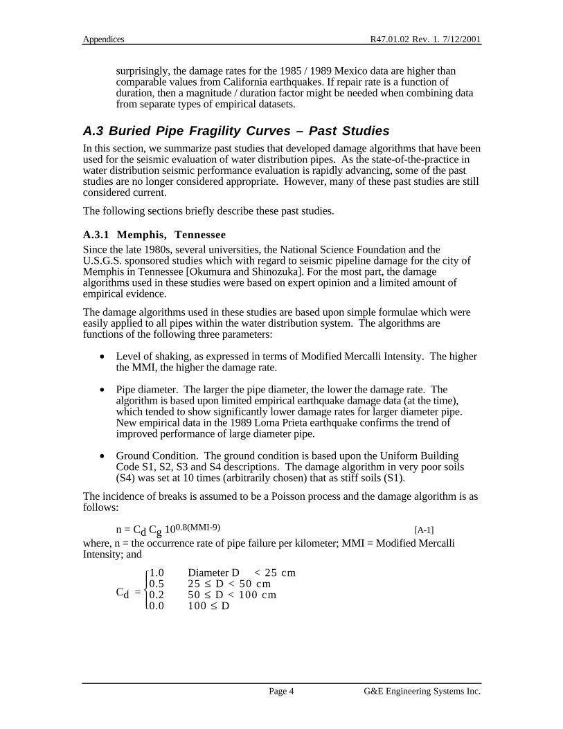
A.3.1 Memphis, TennesseeSince the late 1980s, several universities, the National Science Foundation and theU.S.G.S. sponsored studies which with regard to seismic pipeline damage for the city ofMemphis in Tennessee [Okumura and Shinozuka]. For the most part, the damagealgorithms used in these studies were based on expert opinion and a limited amount ofempirical evidence.

The damage algorithms used in these studies are based upon simple formulae which wereeasily applied to all pipes within the water distribution system. The algorithms arefunctions of the following three parameters:

• Level of shaking, as expressed in terms of Modified Mercalli Intensity. The higherthe MMI, the higher the damage rate.

• Pipe diameter. The larger the pipe diameter, the lower the damage rate. Thealgorithm is based upon limited empirical earthquake damage data (at the time),which tended to show significantly lower damage rates for larger diameter pipe.New empirical data in the 1989 Loma Prieta earthquake confirms the trend ofimproved performance of large diameter pipe.

• Ground Condition. The ground condition is based upon the Uniform BuildingCode S1, S2, S3 and S4 descriptions. The damage algorithm in very poor soils(S4) was set at 10 times (arbitrarily chosen) that as stiff soils (S1).

The incidence of breaks is assumed to be a Poisson process and the damage algorithm is asfollows:

n = Cd Cg 100.8(MMI-9) [A-1]

where, n = the occurrence rate of pipe failure per kilometer; MMI = Modified MercalliIntensity; and

Cd =

1.0 Diameter D < 25 cm0.5 25 ≤ D < 50 cm0.2 50 ≤ D < 100 cm0.0 100 ≤ D

Appendices R47.01.02 Rev. 1. 7/12/2001


Cg =

0.5 Soil S11.0 Soil S22.0 Soil 3S5.0 Soil S4

The probability of a major pipe failure (i.e., complete break with total water loss) iscalculated as:

Pfmajor = 1 - e-nL [A-2]

where L = the length of pipe and n is defined by the equation above.

The occurrence rate of leakage (minor damage) is assumed to be:

Pfminor = 5 Pf major [A-3]

The above damage algorithms are very simple, and capture several of the key features ofhow seismic hazards affect pipe. Although these damage algorithms are simple to use, theyare not considered suitable for “modern” loss estimation efforts as they are based on theMMI scale (instead of PGV and PGD), and omit factors such as pipe construction material,corrosion and amounts (if any) of ground failures.

A.3.2 University-based Seismic Risk Computer ProgramResearchers at Princeton University have developed a program [Sato and Myurata] usingthe same damage algorithm as for Memphis above, except that the Cg factor (ranging from1.0 to 0.0, depending on ground conditions) is omitted.

The damage algorithm presented in the following table is taken from that reference. Notehow the pipe failure rate is strongly dependent upon seismic intensity and pipe diameter.For the same reasons as for the Memphis algorithms, these damage algorithms are notconsidered suitable for use in “modern” loss estimation studies.

MMI Scale D < 25 cm 25 ≤ D < 50 cm 50 ≤ D < 100cm

100 ≤ D

VI 0.003 0.001 0.000 0.000VII 0.025 0.012 0.005 0.000VIII 0.158 0.079 0.031 0.000IX 1.000 0.500 0.200 0.000X 6.309 3.154 1.261 0.000

Table A.3-1. Occurrence Rate of Pipe Failure (per km)

A.3.3 Metropolitan Water DistrictIn a 1978 study on large diameter (40 to 70 inches) welded seamless pipe for the LosAngeles area Metropolitan Water District (MWD) [Shinozuka, Takada and Ishikawa], a setof damage algorithms was developed based upon analytical calculations of strain levels inthe pipe. These algorithms were then applied to the MWD water transmission network.

For wave propagation, the structural strains in the pipe were calculated based upon the freefield soil strains. For segments of pipe that cross through areas where soil liquefaction orsurface fault rupture are known to occur, the pipe strains are computed using formulas by

Appendices R47.01.02 Rev. 1. 7/12/2001


[Newmark and Hall] or [in ASCE, 1984]. A series of damage probability matrices weredeveloped for the various units of soil conditions that the large diameter pipe traverses. Atypical damage probability matrix is as follows.

MMI Scale Minor Damage Moderate Damage Major DamageVI 1.00 0.00 0.00VII 0.96 0.04 0.00VIII 0.18 0.71 0.11IX 0.00 0.11 0.89

Table A.3-2. Damage Probability Matrix

This table applies for pipe with curves and connections in poor soil conditions. ForIntensity VIII, such pipe will have an 18% chance of being undamaged (minor damage), a71% chance of leakage (moderate damage), and an 11% chance of a total break (majordamage).

These algorithms introduce the concept of uncertainty into the analysis. For example,given Intensity IX, there is some uncertainty whether the damage rates will be "moderate"or "major". The uncertainty arises both from imperfect knowledge of the capacity ofindividual pipe strengths and the randomness of the earthquake hazard levels.

A.3.4 San Francisco Auxiliary Water Supply SystemThe damage algorithms suggested by Grigoriu et al [Grigoriu, O’Rourke, Khater] wereused in a study on pipeline damage of the Auxiliary Water Supply System (AWSS) for thecity of San Francisco, California. The AWSS consists of about 115 miles of pipelines withdiameters in the range of 10 to 20 inches.

For modeling expected damage from traveling waves, the authors used a simpler version ofthe Memphis model. For the AWSS, they adopted the following model:

Pf = 1 - e-nL [A-4]

where, Pf = probability that a pipe will have no flow (i.e., complete failure);n = the mean break rate for the pipe; and, L = the length of the pipe.

No damage algorithms were provided for other seismic hazards (e.g., landslides, surfacefaulting, liquefaction - although the San Francisco Liquefaction study, described below,considers liquefaction effects on this system). To obtain the mean break rate, the authorsof this study summarized pipeline damage statistics for traveling wave effects due to fivepast earthquakes.

All pipes, independent of size, age, kind or location, were modeled with the same meanbreak rate value. No "leakage" failure modes were adopted. The range of break ratesstudied was from 0.02 breaks per kilometer, to 0.325 breaks per kilometer, with sixintermediate values. The authors loosely suggest that a break rate of 0.02 / kmcorresponds to about Intensity VII, and a break rate of 0.10 per km corresponds to aboutIntensity VIII.

A.3.5 Seattle, WashingtonThis U.S.G.S. - sponsored study for Seattle, Washington, explicitly differentiates betweenpipe damage caused by ground shaking and soil failure due to liquefaction [Ballantyne,

Appendices R47.01.02 Rev. 1. 7/12/2001


Berg, Kennedy, Reneau and Wu]. This is a major refinement as compared to some earlierefforts.

The authors use the following damage algorithms for ground shaking effects:

n = a eb(MMI - 8) [A-5]where, n = repairs per kilometer, and a and b are adjusted to fit the scatter in empiricalevidence of damage from selected past earthquakes, and engineering judgment. The resultsare shown in Figure A-3.

The damage algorithm for buried pipelines which pass through liquefied soil zones isdescribed in Table A.3-3. This is also shown graphically in Figure A-4. Figures A-4 andA-5 show the suggested landslide and fault crossing algorithms, respectively.

Pipe Kind Repairs (Breaks or Leaks)per Kilometer

Asbestos Cement 4.5Concrete 4.5Cast Iron 3.3PVC 2.6Welded Steel with Caulked Joints 2.6Welded Steel with Gas or Oxyacetylene Welded Joints 2.4Ductile Iron 1.0Polyethylene 0.5Welded Steel with arc-welded joints 0.5

Table A.3-3. Pipe Damage Algorithms Due to Liquefaction PGDs

In application, the authors compute the damage rate using equation A-5 (based on MMI)and the liquefaction-zone rate (based on soil description). The higher of the two rates isapplied to the particular pipe if the pipe is located in a liquefaction zone.

This study also refined some of the historical repair damage statistics to allowdifferentiation between leak and break damage. Undifferentiated damage is denoted asrepairs.

• A leak represents joint failures, circumferential failures (round cracks), andcorrosion-related failures (pinhole and small blow-outs).

• A break represents longitudinal cracks, splits and ruptures. A full circle break ofCast Iron or Asbestos Cement pipe, for example, would also be defined as a break.

By reviewing the damage / repair data from the 1949 and 1969 Seattle, 1969 Santa Rosa,1971 San Fernando Valley, 1983 Coalinga, and 1987 Whittier Narrows earthquakes, thefollowing observations were made:

• In local areas subjected to fault rupture, subsidence, liquefaction or spreadingground, approximately 50% of all recorded repairs/damage have been breaks. Theremaining 50% of all repairs / damage have been leaks.

• In local areas only subjected to traveling wave motions, approximately 15% of allrecorded repairs / damage have been breaks. The remaining 85% of all repairs havebeen leaks.

Appendices R47.01.02 Rev. 1. 7/12/2001


A.3.6 Empirical Vulnerability ModelsIn this National Science Foundation sponsored study performed by the J. H. WigginsCompany [Eguchi et al], empirical-based damage algorithms were developed for pipe inground shaking, fault rupture, liquefaction and landslide areas. They were based onreview of actual pipe damage from the 1971 San Fernando, 1969 Santa Rosa, 1972Managua and the 1979 El Centro earthquakes. The algorithms are statistical in nature bycomputing the number of pipe breaks per 1,000 feet of pipe. The algorithms denotedifferent break rates according to pipe type. Asbestos cement pipe generally was found tohave the poorest performance and welded steel having the best performance. The studyalso indicates that corroded pipe have break rates about three times that of uncorroded pipe.

This empirical evidence forms the basis of some of the more recent efforts, including theSeattle (described above) damage algorithms. The increased repair rate for corroded pipesalso serves as partial basis for the pipeline fragility curves in the current study.

A.3.7 San Francisco Liquefaction StudyIn this study [Porter et al] the repair rate per 1,000 feet of pipe was related to magnitude ofpermanent ground deformation (PGD). Data from the 1989 Loma Prieta (Marina District)and the 1906 San Francisco (Sullivan Marsh and Mission Creek) earthquake were used todevelop a damage algorithm. Figure A-6 shows the algorithm. A key feature is that therepair rate is proportional, at least in some increasing fashion, to the PGD magnitude.

Most of the San Francisco pipe which broke in the liquefied areas in 1906 and 1989 werecast iron.

A.3.8 Empirical Vulnerability Model – Japanese and U.S. DataThis 1975 study [Katayama, Kubo and Sito] developed an empirical pipeline damagemodel based on observed repair rates from actual earthquakes. Several of theseearthquakes were in Japan (1923 Kanto - Tokyo, 1964 Nigata, 1968 Tokachi-Oki).

The repair rate is related to soil condition (good, average, poor), and peak groundacceleration. It does not distinguish between damage caused by ground shaking (wavepropagation), or permanent ground deformations (liquefaction, landslide, fault crossing).Figure A-7 shows the algorithm.

A key conclusion drawn from Figure A-7 is that "poor" to "good" soil conditions bears acritical relationship to overall pipe repair rates. Repair rates in "poor" soils are an order ofmagnitude higher than repair rates in better soils. Another facet to be pointed out is that thisearly effort tried to relate peak ground acceleration to pipe repair rates. More recent effortshave shown that peak ground accelerations is not a good predictor of actual energiesdamaging to pipes. Instead, peak ground velocity (PGV) is a better predictor. PGVs arefurther discussed in the Barenberg work described below.

A.3.9 Wave Propagation Damage Algorithm - BarenbergThis 1988 study [Barenberg] computes a relation between buried cast iron pipe damage(breaks/km) observed in four past earthquakes and peak ground velocities experienced atthe associated sites. The relation is for damage caused by transient ground motions only(i.e., wave propagation effects). Figure A-1 shows the algorithm.

This study makes a major improvement over previous studies. Empirical pipe damage isrelated to actual levels of ground shaking (peak ground velocity) rather than indirect (andvery imperfect) Modified Mercalli Intensity levels. MMIs have often been used in the past,as there were no seismic instruments to record actual ground motions - the MMI scale

Appendices R47.01.02 Rev. 1. 7/12/2001


relates observed items like broken chimneys to ground shaking levels. With the vastlyincreasing number of seismic instruments installed, each future earthquake will add to theempirical database of actual ground motions versus actual observed damage rates.

Another important reason to adopt peak ground velocity as the predictor of ground -shaking induced pipe repairs is that there are mathematical models to relate groundvelocities to strains induced in pipes. This mathematical model states that peak seismicground strain is directly proportional to the peak ground velocity. Up to very high strainlevels the pipes conform to ground movements, and the strain/deformation in the pipe iscorrelated to the ground strain. Hence empirical relations relating damage to peak groundvelocity have a better physical basis than those using Modified Mercalli Intensity.

A.3.10 Wave Propagation Damage Algorithm – O’Rourke and AyalaThis 1988 study [Barenberg] computes a relation between buried cast iron pipe damage(breaks/km) observed in four past earthquakes and peak ground velocities experienced atthe associated sites. The relation is for damage caused by transient ground motions only(i.e., wave propagation effects). Figure A-2 shows the algorithm.

A subsequent work [O’Rourke, M., and Ayala, G., 1994] provides additional empiricaldata points for pipe damage versus peak ground velocity that were not included in theBarenberg work. The additional data are for large diameter (20 and 48 inch diameter)asbestos cement, concrete, prestressed concrete, as well as distribution diameter cast ironand asbestos cement pipe that were subjected to pipe failures in the 1985 Mexico city, 1989Tlahuac and 1983 Coalinga earthquakes.

Some detailed pipe data were lost in the 1985 Mexico earthquake (the water company'sfacility collapsed and records were lost). However, it appears that the bulk of the largediameter transmission pipe that is represented by the data in Figure A-2 is for segmentedAC and concrete pipe. Joints were typically cemented. A least squares regression line (R2 =0.71) is plotted for convenience.

The following observations are made:

1. The empirical evidence (Figures A-1 and A-2) does not clearly suggest a "turn over"point in the damage algorithm, as is suggested in the Seattle study (Figure A-3) at MMI= VIII (or PGV = 20 inches / second after conversion).

2. The empirical data is more severe at very low levels of shaking than suggested in theSeattle study. The differences are smaller at strong levels of shaking. In practice, thismay not be a great concern, as being greatly off at very low levels of shaking probablydoes not meaningfully change the level of overall system damage.

A.3.11 Damage Algorithms – Loma Prieta - EBMUDThis study of the EBMUD water distribution system [Eidinger 1998, Eidinger et al 1995,unpublished work] presents the empirical damage data to over 3,300 miles of pipelines thatwere exposed to various levels of ground shaking in the 1989 Loma Prieta earthquake. Aneffort to collate all pipeline damage from the Loma Prieta and Northridge earthquakes isavailable from http://quake.abag.ca.gov. Using GIS techniques, the entire inventory ofEBMUD pipelines was analyzed to estimate the median level of ground shaking at eachpipe location. Attenuation models used in this study were calibrated to provide estimates ofground motions approximately equal to those observed at 12 recording stations within theEBMUD service area. Then, careful review was made of each damage location where pipesactually were repaired in the first few days after the earthquake (see Figure A-8 for a mapof damage locations).

Appendices R47.01.02 Rev. 1. 7/12/2001


PGV / Material Cast IronRR / 1000 feet

Asbestos CementRR / 1000 feet

Welded SteelRR / 1000 feet

3 Inches / sec 0.00560 0.00341 0.002535 Inches / sec 0.01230 0.00239 0.008417 Inches / sec 0.00517 0.00086 0.0061017 Inches / sec 0.09189 0.01230 0.14826

Table A.3-4. Pipe Repair Rates per 1,000 Feet, 1989 Loma Prieta Earthquake

The damage pipe locations were binned into twelve groups, representing four averagelevels of PGV, and for three types of pipeline: cast iron, asbestos cement (rubber gasketjoints) and welded steel (single lap welded joints). Repair rates were calculated for eachbin. The total inventory of pipelines included about 752 miles of welded steel pipe, 1,008miles of asbestos cement pipe, and 1,480 miles of cast iron pipe. There were 135 piperepairs to the EBMUD system due to the Loma Prieta earthquake. (Mains: 52 cast iron, 46steel, 13 asbestos cement, 2 PVC. Service connections: 22 up to meter – damage oncustomer side of meter not counted). Tables A.3-4 and A.3-5 show the results.

PGV / Material Cast IronMiles of Pipe

Asbestos CementMiles of Pipe

Welded SteelMiles of Pipe

3 Inches / sec 473.2 444.7 374.25 Inches / sec 123.2 79.2 45.07 Inches / sec 878.8 438.3 279.317 Inches / sec 20.6 46.2 60.0

Table A.3-5. Length of Pipe in Each Repair Rate Bin, Loma Prieta Earthquake

The twelve data points from Table A.3-4, are plotted in Figure A-9. An exponential curvefit is drawn through the data. The scatter shown in this plot is not unexpected, in thatdamage data for three different kinds of pipe are all combined into one regression curve.

The same data in Figure A-9 are plotted in Figure A-10, but this time using three differentregression curves, one for each pipe material. Table A.3-6 provides the coefficients for theregression relationships.

Value / Material Cast IronRR / 1000 feet

Asbestos CementRR / 1000 feet

Welded SteelRR / 1000 feet

a 0.000737 0.000725 0.000161b 1.55 0.77 2.29PGV in/sec in/sec in/secR^2 0.71 0.26 0.90

Table A.3-6. Regression Curves for Loma Prieta Pipe Damage, RR = a (PGV)^b, R^2

One issue that is brought out by examining Figures A-9 and A-10 is whether a pipe fragilitycurve should be represented by:

• RR = k a (PGV)b, where k is some set of constants that relate to the specific pipematerial, joinery type, age, etc, and (a,b) are constants developed by the entireempirical pipe database (like Figure A-9); or

Appendices R47.01.02 Rev. 1. 7/12/2001


• RR = a (PGV)^b, where (a,b) are constants specific to the particular pipe type,ideally with all other factors (joinery, age, etc.) being held constant (like Figure A-10).

The standard error terms (R2) in the regression relationships in Table A.3-6 seem "better"than those in Figure A-9. However, this might be because the regression relationships inFigure A-10 use fewer data points (4) than the regression line in Table A.3-6 and Figure A-9 (12). Based on engineering judgment, R2 values like 0.90 for the welded steel pipe curve(Figure A-10) appear to be too high, and are considered more of an artifact of a small dataset than being a true predictor of uncertainty. This statement is made because theperformance of steel pipe is also known to be a factor of age, corrosive soils, quality ofconstruction of the welds, diameter (possibly), etc., which are not accounted for in the twoparameter regression models in Figures A-9 or A-10.

Another key observation from Figure A-10 is that Asbestos Cement pipe (with gasketedjoints) appears to perform better than cast iron or welded steel pipe, at least for damageinduced by ground shaking. This is in contrast to Figure A-3, which ranks welded steelbetter than cast iron, and asbestos cement the worst. As also demonstrated in SectionA.3.12, the same trend is seen in the 1994 Northridge earthquake, where asbestos cementpipe performed better than ductile iron pipe or cast iron pipe. Base on the rigor of theanalyses for the Loma Prieta and Northridge data sets, it would appear that the trend forasbestos cement pipe in Figure A-3 is wrong. This might be due to a reliance onengineering judgment (Figure A-3) for the performance of rubber gasketed AC pipe, as theempirical evidence of AC pipe performance from Loma Prieta and Northridge was notavailable when Figure A-3 was developed.

There has been some researchers that have suggested that pipe damage rates seem to be afunction of pipe diameter (for example, see Section 4.4.7). There is debate as to why thismight or might not be so.

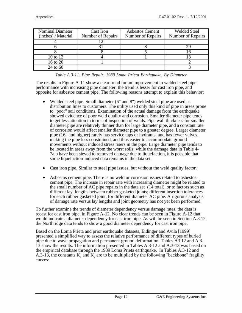
Tables A.3-7, A.3-8 and A.3-9 provide the EBMUD – Loma Prieta database of pipelengths and pipe repairs for cast iron, welded steel and asbestos cement pipe, respectively.Figure A-11 summarizes the empirical evidence for the 1989 Loma Prieta earthquake.Tables A.3-10 and A.3-11 provides the length of pipe and number of repairs for each datapoint in Figure A-11.

Nominal Diameter(inches) / Material

Cast IronMiles of Pipe

Asbestos CementMiles of Pipe

Welded SteelMiles of Pipe

4 3216 784 663 1118 218 296 147

10 to 12 114 49 20816 to 20 43 13624 to 60 151

Table A.3-10. Pipe Lengths, 1989 Loma Prieta Earthquake, By Diameter

Appendices R47.01.02 Rev. 1. 7/12/2001


Nominal Diameter(inches) / Material

Cast IronNumber of Repairs

Asbestos CementNumber of Repairs

Welded SteelNumber of Repairs

4 126 31 8 298 8 5 16

10 to 12 4 1 1316 to 20 1 224 to 60 3

Table A.3-11. Pipe Repair, 1989 Loma Prieta Earthquake, By Diameter

The results in Figure A-11 show a clear trend for an improvement in welded steel pipeperformance with increasing pipe diameter; the trend is lesser for cast iron pipe, andopposite for asbestos cement pipe. The following reasons attempt to explain this behavior:

• Welded steel pipe. Small diameter (6" and 8") welded steel pipe are used asdistribution lines to customers. The utility used only this kind of pipe in areas proneto "poor" soil conditions. Examination of the actual damage from the earthquakeshowed evidence of poor weld quality and corrosion. Smaller diameter pipe tendsto get less attention in terms of inspection of welds. Pipe wall thickness for smallerdiameter pipe are relatively thinner than for large diameter pipe, and a constant rateof corrosion would affect smaller diameter pipe to a greater degree. Larger diameterpipe (16" and higher) rarely has service taps or hydrants, and has fewer valves,making the pipe less constrained, and thus easier to accommodate groundmovements without induced stress risers in the pipe. Large diameter pipe tends tobe located in areas away from the worst soils; while the damage data in Table 4-7a,b have been sieved to removed damage due to liquefaction, it is possible thatsome liquefaction-induced data remains in the data set.

• Cast iron pipe. Similar to steel pipe issues, but without the weld quality factor.

• Asbestos cement pipe. There is no weld or corrosion issues related to asbestoscement pipe. The increase in repair rate with increasing diameter might be related tothe small number of AC pipe repairs in the data set (14 total), or to factors such asdifferent lay lengths between rubber gasketed joints; different insertion tolerancesfor each rubber gasketed joint, for different diameter AC pipe. A rigorous analysisof damage rate versus lay lengths and joint geometry has not yet been performed.

To further examine the trends of diameter dependency versus damage rates, the data isrecast for cast iron pipe, in Figure A-12. No clear trends can be seen in Figure A-12 thatwould indicate a diameter dependency for cast iron pipe. As will be seen in Section A.3.12,the Northridge data tends to show a good diameter dependency for cast iron pipe.

Based on the Loma Prieta and prior earthquake datasets, Eidinger and Avila [1999]presented a simplified way to assess the relative performance of different types of buriedpipe due to wave propagation and permanent ground deformation. Tables A3.12 and A.3-13 show the results. The information presented in Tables A.3-12 and A.3-13 was based onthe empirical database through the 1989 Loma Prieta earthquake. In Tables A.3-12 andA.3-13, the constants K1 and K2 are to be multiplied by the following "backbone" fragilitycurves:

Appendices R47.01.02 Rev. 1. 7/12/2001


Ground shaking: n = 0.00032 (PGV)1.98, (n = repair rate per 1,000 feet of pipe, PGV ininches per second)

Permanent ground deformation: n = 1.03 (PGD)0.53 (n = repair rate per 1,000 feet ofpipe, PGD in inches)

Pipe Material Joint Type Soils Diam. K1 Quality

Cast iron Cement All Small 0.8 BCast iron Cement Corrosive Small 1.1 CCast iron Cement Non corr. Small 0.5 BCast iron Rubber gasket All Small 0.5 DWelded steel Lap - Arc welded All Small 0.5 CWelded steel Lap - Arc welded Corrosive Small 0.8 DWelded steel Lap - Arc welded Non corr. Small 0.3 BWelded steel Lap - Arc welded All Large 0.15 BWelded steel Rubber gasket All Small 0.7 DAsbestos cement Rubber gasket All Small 0.5 CAsbestos cement Cement All Small 1.0 BAsbestos cement Cement All Large 2.0 DConcrete w/Stl Cyl. Lap - Arc Welded All Large 1.0 DConcrete w/Stl Cyl. Cement All Large 2.0 DConcrete w/Stl Cyl. Rubber Gasket All Large 1.2 DPVC Rubber gasket All Small 0.5 CDuctile iron Rubber gasket All Small 0.3 C

Table A.3-12. Ground Shaking - Constants for Fragility Curve (after Eidinger)

Pipe Material Joint Type K2 Quality

Cast iron Cement 1.0 BCast iron Rubber gasket, mechanical 0.7 CWelded steel Arc welded, lap welds 0.15 CWelded steel Rubber gasket 0.7 DAsbestos cement Rubber gasket 0.8 CAsbestos cement Cement 1.0 CConcrete w/Stl Cyl. Welded 0.8 DConcrete w/Stl Cyl. Cement 1.0 DConcrete w/Stl Cyl. Rubber Gasket 1.0 DPVC Rubber gasket 0.8 CDuctile iron Rubber gasket 0.3 C

Table A.3-13. Permanent Ground Deformations - Constants for Fragility Curve (afterEidinger)

Eidinger suggested a "quality" factor ranging from B to D. "B" suggested reasonableconfidence in the fragility curve based on empirical evidence; "D" suggested littleconfidence.

The empirical evidence from the 1994 Northridge earthquake (see Section A.3.12) suggeststhat K1 for small diameter AC pipe might be about 0.4 times that for cast iron pipe;similarly K1 for small diameter ductile iron pipe might be around 0.55. The K1 constant forPVC pipe might be similar to that for AC pipe (0.4), still recognizing the lack of empiricaldata for PVC pipe. The relative performance of different pipe materials in the Kobeearthquake (Figure A-17) seems to support that DI pipe has a moderately lower break rate

Appendices R47.01.02 Rev. 1. 7/12/2001


than the "average" pipe material, but possibly only about 50% lower than the average. Thepoor performance of small diameter screwed steel pipe in the Northridge earthquake wouldsuggest a K1 value of between 1.1 and 1.5 for that kind of pipe.

A.3.12 Wave Propagation Damage Algorithms – 1994 Northridge – LADWPA GIS-based analysis of the pipeline damage to the LADWP water system was performedby [after T. O'Rourke and Jeon, 1999]. This GIS analysis is based on the following:

• Data reported herein are for cast iron, ductile iron, asbestos cement and steel pipe,up to 24" in diameter. The pipeline inventory includes: 7,848 km of cast iron pipe;433 km of ductile iron pipe; and 961 km of asbestos cement pipe.

• A total of 1,405 pipe repairs were reported for the LADWP distribution systembased on work orders. Of these, 136 were removed from the statistics, either beingdue to damage to service line connections on the customer side of meter; non-damage for any other reason (the work crew could not find the leak after theyarrived at the site); duplications; non-pipe related. An additional 208 repairs wereremoved from the statistics, being caused by damage to service connections on theutility side of the meter, at locations without any damage to the pipe main. Anadditional 48 repairs are removed from the statistics, being for pipes with diameters24" and larger. Also, 74 repairs were removed from the statistics, as either pipelocations, type or size was unknown at these locations (this introduces a downwardbias in the raw damage rates of 7.9% = 74 / 939). The remaining pipe data locationsare: 673 repairs for cast iron pipe; 24 repairs for ductile iron pipe; 26 repairs forasbestos cement pipe, 216 repairs for steel pipe.

• Note: Repair data in Section A.3.11 (Loma Prieta) does not remove service lineconnection repairs, which represent 19.5% (= 22 / 113) of the repairs due to mains.Repair data in A.3.12 (Northridge) does remove service line connection repairs,which represent 20.5% (= 208 / 1,013) of the repairs due to mains. This suggeststhat the quantity of repairs to service line connections would be about 20% that formains. The Loma Prieta database includes pipe material, diameter and location atevery location; the Northridge database has one or more of these attributes missingat 7.9% of all locations and this data was omitted from the statistical analyses.Combining damage data between the two data sets (Loma Prieta and Northridge)needs to adjust for these difference (total about 28% difference).

• Damage to steel pipelines in the Northridge database of distribution pipelines wasabout 216 repairs. The average damage rate for steel pipe was twice as high as thatfor all other types of pipe combined. The reasons for this are several:

- Steel pipelines are concentrated in hillsides and mountains, owing to adesign philosophy that steel pipes should be used rather than cast iron pipesin hillside terrain.

- Several types of steel pipe are included in the "steel" category,including(as reported by O'Rourke and Jeon): welded joints (43%);screwed joints (9%); elastomeric or victaulic coupling joints (7%); pipeswith and without corrosion protection (coatings, sacrificial anodes,impressed current), pipes using different types of steel, includingMannesman and Matheson steel (30%) which are known to be prone tocorrosion; and riveted pipe (1%). Pending more study of the steel pipelinedatabase, repairs to these pipes have not yet been completely evaluated byT. O'Rourke and this data is not incorporated into the fragility formulations

Appendices R47.01.02 Rev. 1. 7/12/2001


in this report. Percentages in this paragraph pertain to the percentage of allsteel pipe repairs with the listed attribute. Mannesman and Matheson steelpipes were installed mostly in the 1920s and 1930s without cement liningand coating, and have wall thicknesses generally thinner than moderninstalled steel pipes of the same diameter.

- 4" diameter steel pipe use screwed fittings; 6" and larger steel pipe usewelded slip joints.

• Pipe damage in locales subjected to large PGDs have been "removed" from thedatabase.

• Pipe damage data were correlated (by T. O'Rourke and Jeon) with peakinstrumented PGV to the nearest recording (peak instrumented was the highest ofthe two orthogonal recorded horizontal motions, not the vector maximum). Mostother data in this report is presented with regards to the average of the peak groundvelocities from two orthogonal directions. This is commonly the measure of groundvelocity provided by attenuation relationships.

A comparison of instrumental records revealed that the ratio of peak horizontal velocity tothe average peak velocity from the two orthogonal directions was 1.21. Accordingly, wepresent in this report "corrected" PGV data from the original work (except note that thiscorrection was not applied to the dataset used in Appendix G).

Unpublished work suggests that R2 coefficients are higher if pipe damage from theNorthridge earthquake is correlated with the vector maximum of the two horizontalrecorded PGVs.

Appendices R47.01.02 Rev. 1. 7/12/2001


Tables A.3-14, A.3-15 and A.3-16 summarizes the results. The data set included 4,900miles of Cast Iron pipe (mostly 4", 6" and 8" diameter, with about 15% of the total for 10"through 24" diameter), 270 miles of Ductile Iron pipe (4", 6", 8" and 12" diameter) and600 miles of Asbestos Cement pipe (4", 6" and 8" diameter). In order to maintain aminimum length of pipe for each reported statistic, each reported value is based on aminimum length of about 80 miles (cast iron pipe) or 13 miles (ductile iron and asbestoscement). This is done to smooth out spurious repair rate values if the length of pipe in anysingle bin is very small. At higher PGV values, this required digitization at slightlydifferent PGV values for AC and DI pipe.

PGV (inches/sec)Cast Iron

RR / 1000 feetCast Iron

Miles of PipeCast IronRepairs

1.6 0.0 156.8 04.9 0.0079 1055.8 448.1 0.0230 1370.7 166

11.4 0.0300 699.7 11114.6 0.0221 503.1 5917.9 0.0337 313.9 5621.1 0.0739 222.7 8724.4 0.0662 111.7 3927.7 0.0540 87.6 2432.5 0.0064 117.6 439.0 0.0205 101.8 1145.6 0.0246 84.8 1152.1 0.1441 78.9 60

Table A.3-14. Pipe Repair Data, Cast Iron Pipe, 1994 Northridge Earthquake

PGV (inches/sec)Asbestos Cement

RR / 1000 feetAsbestos Cement

Miles of PipeAsbestos Cement

Repairs1.6 0.0 98.3 04.9 0.0020 192.4 28.1 0.0193 147.2 15

11.4 0.0051 73.6 214.6 0.0 23.6 017.9 0.0 21.3 021.1 0.0873 15.2 729.3 0.0 13.4 035.8 0.0 15.8 0

Table A.3-15. Pipe Repair Data, Asbestos Cement Pipe, 1994 Northridge Earthquake

Appendices R47.01.02 Rev. 1. 7/12/2001


PGV (inches/sec)Ductile Iron

RR / 1000 feetDuctile IronMiles of Pipe

Ductile IronRepairs

1.6 0.0 26.4 04.9 0.0026 72.9 18.1 0.0196 57.9 6

11.4 0.0150 25.2 214.6 0.0282 20.1 317.9 0.0167 11.3 122.8 0.0887 12.8 629.3 0.0283 13.4 235.8 0.0131 14.4 147.2 0.0236 16.1 2

Table A.3-16. Pipe Repair Data, Ductile Iron Pipe, 1994 Northridge Earthquake

Figure A-13 shows the "backbone" regression curve. The R2 value is low (0.26),suggesting that by combining all damage data into one plot leads to substantial scatter.

Figure A-14 compares the Loma Prieta (solid line) and Northridge (dashed line) backbonecurves. As previously discussed, the Loma Prieta curve includes damage to serviceconnections (about 20%), and the Northridge curve excludes damage due toincompleteness in the damage data set (about 8%). Also, the Loma Prieta database includescast iron, asbestos cement and steel; the Northridge database include cast iron, asbestoscement and ductile iron. Given these differences, the two curves are not that different: i.e.,the curves are mostly within 50% of each other.

A significant concern in developing regression curves of the sort shown in Figures A-9through A-14 is that the "data points" are based on rates of damage. As such, one datapoint which is based on 100 miles of pipe is given the same influence as another data pointwhich is based on 20 miles of pipe. Also, data points which have "0" repair rate cannot beincluded in an exponential-based regression curve. One approach to handle this problem istreated using a Bayesian form of curve fitting, as outlined in Appendix G. Another way toaddress this is to "weight" the repair data statistics such that each point represents an equallength of pipe. By "weighting", it is meant that the regression analysis is performed with 5data points representing a sample with 100 miles of pipe, and 1 data point representing asample with 20 miles of pipe. The results of the "weighted" analysis are shown in FigureA-15. In developing Figure A-15, the Loma Prieta and Northridge data are normalized toaccount of the way the raw data was developed (service connections, missing main repairdata). The main effects of the weighting are as follows:

• The influence of smaller samples of pipe, at the higher PGV levels, has less influenceon the regression coefficients.

• The regression curve using a weighted sample is almost linear (power coefficient =0.99).

Figure A-16 shows a regression analysis (unweighted) for asbestos cement pipe for boththe Loma Prieta and Northridge datasets.

Based on comparable levels of shaking, the relative vulnerability of each pipe material (justNorthridge data) was evaluated. Table A.3-17 shows the results.

Appendices R47.01.02 Rev. 1. 7/12/2001


PGV(inch/sec)

CastIronRR /1000feet

AsbestosCement

RR / 1000 feet

DuctileIronRR /1000feet

Average

RR /1000feet

CI /Average

AC /Average

DI /Average

5.9 0.0079 0.0020 0.0026 0.0041 1.902 0.476 0.6229.8 0.0230 0.0197 0.0197 0.0208 1.105 0.948 0.94813.8 0.0300 0.0052 0.0152 0.0168 1.790 0.307 0.90317.7 0.0221 0.0288 0.0255 0.869 1.13121.7 0.0337 0.0167 0.0252 1.338 0.66225.6 0.0739 0.0894 0.0939 0.0857 0.861 1.043 1.096

Average 1.311 0.693 0.894

Table A.3-17. Pipe Repair Data, 1994 Northridge Earthquake

This suggests the relative vulnerability of these three pipe materials, from the Northridgeearthquake for areas subjected to ground shaking and no PGDs, as follows:

• Cast Iron. 30% more vulnerable than average.

• Asbestos Cement. 30% less vulnerable than average

• Ductile Iron. 10% less vulnerable than average.

A.3.13 Relative Pipe Performance – BallantyneBallantyne presents a model to consider the relative performance of pipelines in earthquakeswhich differentiates between the properties of the pipe barrel from the pipe joint.

• Pipe joints usually fail from extension (pulled joints); compression (split ortelescoped joints); or bending or rotation.

• Pipe barrels usually fail from shear; bending; holes in the pipe wall, or splits.

Holes in pipe walls are usually the result of corrosion. Steel or iron pipe can be weakenedby corrosion; asbestos cement pipe by decalcification, and PVC pipe by fatigue.

Appendices R47.01.02 Rev. 1. 7/12/2001


Given these issues, Ballantyne rates various pipe types using four criteria: ruggedness(strength and ductility of the pipe barrel); resistance to bending failure; joint flexibility; andjoint restraint. Table A.3-18 presents his findings (1 = low seismic capacity, 5 = highseismic capacity).

Material Type/ diameter

AWWAStandard

Joint Type

Rug

gedn

ess

Be

nd

ing

Join

tF

lexi

bili

ty

Re

stra

int

To

tal

Polyethylene C906 Fusion 4 5 5 5 19Steel C2xx series Arc Welded 5 5 4 5 19Steel None Riveted 5 5 4 4 18Steel C2xx series B&S, RG, R 5 5 4 4 18Ductile Iron C1xx series B&S, RG, R 5 5 4 4 18Steel C2xx B&S, RG,

UR5 5 4 1 15

Ductile iron C1xx series B&S, RG,UR

5 5 4 1 15

Concrete withsteel cylinder

C300, C303 B&S, R 3 4 4 3 14

PVC C900, C905 B&S, R 3 3 4 3 13Concrete withsteel cylinder

C300, C303 B&S, UR 3 4 1 12

AC > 8"diameter

C4xx series Coupled 2 4 5 1 12

Cast Iron >8" diameter

None B&S, RG 2 4 4 1 11

PVC C900, C905 B&S, UR 3 3 4 1 11Steel None Gas welded 3 3 1 2 9AC ≤ 8"diameter

C4xx series Coupled 2 1 5 1 9

Cast iron ≤8" diameter

None B&S, RG 2 1 4 1 8

Cast iron None B&S, rigid 2 2 1 1 6B&S = Bell and spigot. RG = rubber gasket. R = restrained. UR = unrestrained

Table A.3-18. Relative Earthquake Vulnerability of Water Pipe

By comparing the rankings in Tables A.3-18 versus those in Tables A.3-12 and A.3-13,we see the following trends:

• Both tables rank welded steel pipe as about the best pipe. Table A.3-12 providessubstantial downgrades for cases were corrosion is likely, and the evidence fromthe Northridge and Loma Prieta earthquakes strongly indicates that corrosion is animportant factor.

• Table A.3-18 presents high density polyethylene pipe (HDPE) as being veryrugged. To date, there is essentially no empirical evidence of HDPE performance inwater systems, but it appears to have performed well in gas distribution systems.Limited tests on pressurized HDPE pipe have shown strain capacities before leak inexcess of 25% (tensile) and 10% (compression), which suggests very goodruggedness. HDPE pipe is not susceptible to corrosion. There remains some

Appendices R47.01.02 Rev. 1. 7/12/2001


concern about the long term use of resistance of HDPE pipe to intrusion of certainoil-based compounds; should this issue be adequately resolved, then the use ofHDPE pipe in areas prone to PGDs may be very effective in reducing pipe damage.

• Table A.3-18 suggests that unrestrained ductile iron pipe is more rugged than ACpipe; this reflects common assumptions about the ductility of DI pipe, but in somecases does not match the empirical evidence (Northridge 1994), where AC pipeperformed better than DI pipe.

Ballantyne suggests that in high seismic zones (Z ≥ 0.4g), DI pipe (restrained joints), steelpipe (welded or restrained joints); HDPE with fusion welded joints should be used. Forpurposes of this report, these recommendations appear sound, although the use of thesematerials might best be considered for any seismically active region (Z ≥ 0.15g) with localsoils prone to PGDs; and in the areas with high PGVs (Z ≥ 0.4g), the use of rubbergasketed (short barrel length, long joint insertions) AC, DI or PVC pipe might still yieldacceptably good performance.

A.3.14 Pipe Damage Statistics – 1995 Kobe EarthquakeThe 1995 Hanshin-Awaji earthquake (often called the Hyogo-Ken Nanbu (Kobe)earthquake) was a M 6.7 crustal event that struck directly beneath much of the urbanizedcity of Kobe, Japan. At the time of the earthquake, the pipeline inventory for the City ofKobe’s water system included 3,180 km of Ductile Iron pipe (push on joint), 237 km ofspecial Ductile Iron pipe (with special flexible restrained joints), 103 km of high pressuresteel welded pipe, 309 km of cast iron pipe with mechanical joints, and 126 km of PVCpipe with push-on gasketed joint [Eidinger et al, 1998].

The City of Kobe’s water system suffered 1,757 pipe repairs to mains. The averagedamage rate to pipe mains was 0.439 repairs per km. The repairs could be classified intoone of three types: damage to the main pipe barrel (splitting open); damage to the pipe joint(separated); damage to air valves and hydrants; the damage rate was divided about 20% -60% - 20% for these three types of repairs, respectively. Average pipe repair rates wereabout 0.2/km (PVC pipe); 1.3/km (CI pipe); 0.25/km (Ductile Iron pipe with push on orregular restrained joints); and 0.15/km for welded steel pipe.

Figure A-17 shows the damage rates for pipelines in Kobe, along with the wavepropagation damage algorithm Tables A.3-4, A.3-14, A.3-15, A.3-16 and Figures A-1 andA-2. The Kobe data is plotted as horizontal lines; meaning the data is not differentiated bylevel of ground shaking. Also, the Kobe data is not differentiated between damage fromPGVs or PGDs. Note that while the ratio of damage between pipeline materials for Kobe isknown, to say that one pipe material is that much better than the next may be misleading, asthe inventory of different pipe materials may have been exposed to differing levels ofhazards. There remains a need to perform a GIS evaluation for the Kobe pipe inventory in amanner similar to that done for Loma Prieta 1989 (Section A.3.11) or Northridge 1994(Section A.3.12). Shirozu et al [1996] have performed an analysis of the Kobe dataset, andtheir findings are included in the dataset used for evaluation of the PGV-based pipelinefragility curves; Table A.3-19 provides a complete breakdown of the pipe damage for thisearthquake.

There were an additional 89,584 service line repairs in Kobe [Matsushita]. The service linefailure rate was 13.8% of all service lines in the city. The high rate of damage to serviceline connections reflects the large number of structures and roadways that were damaged ordestroyed in the earthquake.

The Cities of Kobe and Ashiya had recently installed a special type of ductile iron pipe (socalled "S and SII joint pipe". A total inventory of 270 km of this type of pipeline was

Appendices R47.01.02 Rev. 1. 7/12/2001


installed at the time of the earthquake, and there was no reported damage to this type ofpipeline. The key features of this type of pipeline were: ductile iron body; with restrainedslip joints at every fitting. Each joint could extent and rotate a moderate amount. This typeof pipeline was installed at about a 50% cost premium to regular push-on type joint ductileiron pipeline.

In the neighboring city of Ashiya, the pipeline inventory included 192 km of pipelines.This included 58 km of Ductile Iron pipe with restrained joints, 96 km of Cast Iron pipe, 2km of steel pipe, 23 km of PVC pipe and 14 km of special Ductile Iron pipe (with flexiblerestrained joints). There were 303 pipe repairs made for this water system (average 1.58repairs / km = 0.48 repairs / 1,000 ft) [Eidinger et al, 1998]. The higher damage rate forAshiya than for Kobe is partially explained in that 100% of Ashiya was exposed to strongground shaking, whereas perhaps only 2/3 of Kobe was similarly exposed; also, Ashiyahas a somewhat higher percentage of Cast Iron pipe.

A.3.15 Pipe Damage Statistics – Recent EarthquakesThe damage to water system pipelines in recent (1999 – 2001) earthquakes is brieflysummarized in this section. As of the time of writing this report, sufficiently accuratedatabases of the pipe damage were unavailable in order for the data to be included in thestatistical analyses presented in this report.

1999 Kocaeli – Izmit (Turkey) EarthquakeThe MW 7.4 Kocaeli (Izmit) earthquake of August 17, 1999 in Turkey led to widespreaddamage to water transmission and distribution systems that serve a population of about1,500,000 people. Potable water was lost to the bulk of the population immediately afterthe earthquake, largely due to damage to buried pipelines.

The most common inventories of pipe material were welded steel pipe (large diametertransmission pipelines) and rubber gasketed asbestos cement pipe (most distributionpipelines).

There was heavy damage to both transmission and distribution pipelines by thisearthquake. Some of the damage was due to rupture at fault offset, some was due towidespread liquefaction, and some was due to strong ground shaking.

At this time, no precise inventory of pipeline damage is available. However, based on thelevel of efforts of crews to repair water pipelines, and the percentage of water servicerestored as of three weeks after the earthquake, it would be reasonable to assume thatbetween 1,000 and 3,000 pipe repairs would be required to completely restore waterservice. An average repair rate possibly in the range of 0.5 to 1/km was likely to haveoccurred in the strongest shaking areas, including the cities of Adapazari and Golcuk, andthe town of Arifye.

1999 Chi-Chi (Taiwan) EarthquakeThe MW 7.7 Chi-Chi (Ji-Ji) earthquake of September 21, 1999 in Taiwan led to 2,405deaths and 10,718 injuries. Potable water was lost to 360,000 households immediatelyafter the earthquake, largely due to damage to buried pipelines.

There was about 32,000 km of water distribution pipelines in the country; perhaps a quarteror more was exposed to strong ground shaking. The largest pipes (diameter ≥1.5 meters)are typically concrete cylinder pipe or steel, with ductile iron pipe being the predominantmaterial for moderate diameter pipe and a mix of polyethylene and ductile iron pipe fordistribution pipe (≤8 inch diameter).

Appendices R47.01.02 Rev. 1. 7/12/2001


At this time, there is incomplete analysis of the damaged inventory to pipelines in thisearthquake. However, the following trends have been observed from preliminary data[Shih et al, 2000]:

• About 48% of all buried water pipe damage is due to ground shaking (this ratio maychange under future analysis). The remainder is due to liquefaction (2%), groundcollapse (11%), ground cracking and opening (10%), horizontal groundmovements (9%), vertical ground movement (16%), other (4%).

• For the town of Tsautuen, repair rates varied from 0.4/km to 7/km (PGA = 0.2g) toas high as 0.6/km (PGA = 0.6g).

2001 Gujarat Kutch (India) EarthquakeThe MW 7.7 Gujarat (Kutch) earthquake of January 26, 2001 in India led to about 17,000deaths and about 140,000 injuries. Potable water was lost to over 1,000,000 peopleimmediately after the earthquake, largely due to damage to wells, pump station buildingsand buried pipelines.

There was about 3,500 km of water distribution and transmission pipelines in the KutchDistrict; perhaps 2,500 km was exposed to strong ground shaking. As of the time ofwriting this report, it is estimated that about 700 km of these pipelines will have to bereplaced due to earthquake damage. It may take up to 4 months after the earthquake tocomplete the pipe repairs.

A.4 ReferencesASCE, 1984, Guidelines for the Seismic Design of Oil and Gas Pipeline Systems,prepared by the ASCE Technical Council on Lifeline Earthquake Engineering, D. NymanPrincipal Investigator, 1984.

Ayala, G. and O'Rourke, M., "Effects of the 1985 Michoacan Earthquake on WaterSystems and other Buried Lifelines in Mexico," National Center for EarthquakeEngineering Report No. 89-009, 1989.

Ballantyne, D. B., Berg, E., Kennedy, J., Reneau, R., and Wu, D., "Earthquake LossEstimation Modeling of the Seattle Water System," Report to U.S. Geological Survey,Grant 14-08-0001-G1526, October 1990.

Barenberg, M.D., "Correlation of Pipeline Damage with Ground Motion," Journal ofGeotechnical Engineering, ASCE, Vol. 114, No. 6, June 1988.

Eguchi, R., T., Legg, M.R., Taylor, C. E., Philipson, L. L., Wiggins, J. H.,"Earthquake Performance of Water and Natural Gas Supply System," J. H. WigginsCompany, NSF Grant PFR-8005083, Report 83-1396-5, July 1983.

Eidinger, J., Maison, B. Lee, D., Lau, R, "EBMUD Water Distribution Damage in the1989 Loma Prieta Earthquake," 4th U.S. Conference on Lifeline Earthquake Engineering,TCLEE, ASCE, San Francisco, 1995.

Eidinger, J. "Lifelines, Water Distribution System," in The Loma Prieta, California,Earthquake of October 17, 1989, Performance of the Built Environment - Lifelines, USGeological Survey Professional Paper 1552-A, pp A63-A80, A. Schiff Ed. December1998.

Eidinger, J., Lund, LeVal and Ballantyne, Don, Water and Sewer Systems, in Hyogo-KenNanbu (Kobe) Earthquake of January 17, 1995, TCLEE Monograph 14, ASCE, 1998.

Appendices R47.01.02 Rev. 1. 7/12/2001


Eidinger, J., Avila, E., eds., Guidelines for the Seismic Upgrade of Water TransmissionFacilities , ASCE, TCLEE Monograph No. 15, January 1999.

Grigoriu, M., O'Rourke, T., Khater, M., "Serviceability of San Francisco Auxiliary WaterSupply System" Proceedings of 5th International Conference on Structural Safety andReliability, San Francisco, California 1989.

Hovland, H. J., and Daragh, R. D. "Earthquake-Induced Ground Movements in theMission Bay Area of San Francisco in 1906," Proceedings of the 2nd Specialty Conferenceof the Technical Council on Lifeline Earthquake Engineering. ASCE, August 1981.

Katayama, T., Kubo, K., and Sito, N., "Earthquake Damage to Water and GasDistribution Systems," Proceedings—U.S. National Conference on EarthquakeEngineering, EERI, 1975.

Manson, M., "Reports on an Auxiliary Water Supply System for Fire Protection for SanFrancisco, California," Report of Board of Public Works, San Francisco, California 1908.

Matsushita, M., Restoration Process of Kobe Water system from the 1995 Hanshin-AwajiEarthquake, in Optimizing Post-Earthquake System Reliability, Proceedings of the 5th USConference on Lifeline Earthquake Engineering, TCLEE Monograph 16, ASCE, August,1999.

McCaffery, M. A., and O'Rourke, T. D., "Buried Pipeline Response to Reverse FaultingDuring the 1971 San Fernando Earthquake," Earthquake Behavior and Safety of Oil andGas Storage Facilities, Buried Pipelines an Equipment, PVP-Vol.77, New York, ASME,1983.

Newmark, N.M., and Hall, W. J.,"Pipeline Design to Resist Large Fault Displacement,"Presented at the June 1975 U. S. National Conference of Earthquake Engineering, AnnArbor, Michigan.

O’Rourke, M.J., and Ayala, G., 1993, Pipeline Damage to Wave Propagation, Journal ofGeotechnical Engineering, ASCE, Vol. 119, No. 9, 1993.

O'Rourke, T.D., and Jeon, S-S., Factors Affecting the Earthquake Damage of WaterDistribution Systems, in Optimizing Post-Earthquake Lifeline System Reliability, TCLEEMonograph No. 16, ASCE, 1999.

O'Rourke, T. D., and Tawfik, M.S. "Effects of Lateral Spreading on Buried PipelinesDuring the 1971 San Fernando Earthquake," Earthquake Behavior and Safety of Oil andGas Storage Facilities, Buried Pipelines and Equipment, PVC,-Vol.77, New York,ASME, 1983.

Porter, K.A., Scawthorn C., Honegger, D. G., O'Rourke, T.D., and Blackburn, F.,"Performance of Water Supply Pipelines in Liquefied Soil," Proceedings—4th U.S.-JapanWorkshop on Earthquake Disaster Prevention for Lifeline Systems, NIST SpecialPublication 840, August 1992.

Sato, Ryo and Myurata, Masahiko, GIS-Based Interactive and Graphic Computer Systemto Evaluate Seismic Risks on Water Delivery Networks, Dept. of Civil Engineering andOperations Research, Princeton University, December 1, 1990.

Schussler, H., "The Water Supply System of San Francisco, California" Spring ValleyWater Company, San Francisco, California, July, 1906.

Appendices R47.01.02 Rev. 1. 7/12/2001


Shih, B., Chen, W., Hung, J-H., Chen, C-W., Wang, P-H., Chen, Y-C., and Liu, S-Y.,The Fragility Relations of Buried Water and Gas Pipes, International Workshop on AnnualCommemoration of Chi-chi Earthquake, Taipei, September 18-20. 2000.

Shinozuka, M. Takada, S. Ishikawa, H., Seismic Risk Analysis of Underground LifelineSystems With the Aid of Damage Probability Matrices , NSF-PFR-78-15049-CU-2,Columbia University, September 1978.

Shirozu, T., Yune, S., Isoyama, R., and Iwamoto, T., “Report on Damage to WaterDistribution Pipes Caused by the 1995 Hyogoken-Nanbu (Kobe) Earthquake,”Proceedings from the 6th Japan-U.S. Workshop on Earthquake Resistant Design of LifelineFacilities and Countermeasures Against Soil Liquefaction, National Center for EarthquakeEngineering Research Report NCEER-96-0012, September 1996.

Toprak, Selcuk, "Earthquake effects on buried pipeline systems," PhD Dissertation,Cornell University, August, 1998.

Wang, Leon, Shao-Ping S.,and Shijie S., "Seismic Damage Behavior of Buried PipelineSystems During Recent Severe Earthquakes in U.S., China and Other Countries, ODULEE-02, Old Dominion University, December 1985.

Wang, L., "A New Look Into the Performance of Water Pipeline Systems From 1987Whittier Narrows, California Earthquake," Department of Civil Engineering, Old DominionUniversity, No. ODU LEE-05, January 1990.

Youd, T. L. and Hoose, S. N. "Historic Ground Failures in Northern CaliforniaAssociated with Earthquakes," Geological Survey Professional Paper No. 993. U.S.Geological Survey, Washington D. C. GPO 1978.

R47.01.02 Rev. 0

ID Earthquake Material Type

Size Length Repairs Rate Demand Comment Source

1001 1995 Hyogoken-nanbu MX DS NR NR 0.031 PGA = 0.211 Includes DI & CI from 1011 to 1029 Shirozu et al, 1996 (Fig. 15)1002 1995 Hyogoken-nanbu MX DS NR NR 0.207 PGA = 0.306 Includes DI & CI from 1011 to 1029 Shirozu et al, 1996 (Fig. 15)1003 1995 Hyogoken-nanbu MX DS NR NR 0.047 PGA = 0.478 Includes DI & CI from 1011 to 1029 Shirozu et al, 1996 (Fig. 15)1004 1995 Hyogoken-nanbu MX DS NR NR 0.057 PGA = 0.572 Includes DI & CI from 1011 to 1029 Shirozu et al, 1996 (Fig. 15)1005 1995 Hyogoken-nanbu MX DS NR NR 0.227 PGA = 0.595 Includes DI & CI from 1011 to 1029 Shirozu et al, 1996 (Fig. 15)1006 1995 Hyogoken-nanbu MX DS NR NR 0.227 PGA = 0.677 Includes DI & CI from 1011 to 1029 Shirozu et al, 1996 (Fig. 15)1007 1995 Hyogoken-nanbu MX DS NR NR 0.062 PGA = 0.710 Includes DI & CI from 1011 to 1029 Shirozu et al, 1996 (Fig. 15)1008 1995 Hyogoken-nanbu MX DS NR NR 0.202 PGA = 0.792 Includes DI & CI from 1011 to 1029 Shirozu et al, 1996 (Fig. 15)1009 1995 Hyogoken-nanbu MX DS NR NR 0.522 PGA = 0.819 Includes DI & CI from 1011 to 1029 Shirozu et al, 1996 (Fig. 15)1010 1995 Hyogoken-nanbu MX DS NR NR 0.098 PGA = 0.834 Includes DI & CI from 1011 to 1029 Shirozu et al, 1996 (Fig. 15)1011 1995 Hyogoken-nanbu DI DS NR NR 0.092 PGA = 0.306 Shirozu et al, 1996 (Fig. 16a)1012 1995 Hyogoken-nanbu DI DS NR NR 0.016 PGA = 0.478 Shirozu et al, 1996 (Fig. 16a)1013 1995 Hyogoken-nanbu DI DS NR NR 0.02 PGA = 0.572 Shirozu et al, 1996 (Fig. 16a)1014 1995 Hyogoken-nanbu DI DS NR NR 0.14 PGA = 0.595 Shirozu et al, 1996 (Fig. 16a)1015 1995 Hyogoken-nanbu DI DS NR NR 0.149 PGA = 0.677 Shirozu et al, 1996 (Fig. 16a)1016 1995 Hyogoken-nanbu DI DS NR NR 0.027 PGA = 0.710 Shirozu et al, 1996 (Fig. 16a)1017 1995 Hyogoken-nanbu DI DS NR NR 0.054 PGA = 0.792 Shirozu et al, 1996 (Fig. 16a)1018 1995 Hyogoken-nanbu DI DS NR NR 0.2 PGA = 0.819 Shirozu et al, 1996 (Fig. 16a)1019 1995 Hyogoken-nanbu DI DS NR NR 0.065 PGA = 0.834 Shirozu et al, 1996 (Fig. 16a)1020 1995 Hyogoken-nanbu CI DS NR NR 0.099 PGA = 0.211 Shirozu et al, 1996 (Fig. 16b)1021 1995 Hyogoken-nanbu CI DS NR NR 0.288 PGA = 0.306 Shirozu et al, 1996 (Fig. 16b)1022 1995 Hyogoken-nanbu CI DS NR NR 0.252 PGA = 0.478 Shirozu et al, 1996 (Fig. 16b)1023 1995 Hyogoken-nanbu CI DS NR NR 0.171 PGA = 0.572 Shirozu et al, 1996 (Fig. 16b)1024 1995 Hyogoken-nanbu CI DS NR NR 0.585 PGA = 0.595 Shirozu et al, 1996 (Fig. 16b)1025 1995 Hyogoken-nanbu CI DS NR NR 0.441 PGA = 0.677 Shirozu et al, 1996 (Fig. 16b)1026 1995 Hyogoken-nanbu CI DS NR NR 0.099 PGA = 0.710 Shirozu et al, 1996 (Fig. 16b)1027 1995 Hyogoken-nanbu CI DS NR NR 1.098 PGA = 0.792 Shirozu et al, 1996 (Fig. 16b)1028 1995 Hyogoken-nanbu CI DS NR NR 1.458 PGA = 0.819 Shirozu et al, 1996 (Fig. 16b)1029 1995 Hyogoken-nanbu CI DS NR NR 0.189 PGA = 0.834 Shirozu et al, 1996 (Fig. 16b)1030 1994 Northridge DI DS 16.1 2 0.0236 PGV = 47.2 LADWP ALA Report Table 4-101031 1994 Northridge DI DS 14.4 1 0.0131 PGV = 35.8 LADWP ALA Report Table 4-101032 1994 Northridge DI DS 13.4 2 0.0283 PGV = 29.3 LADWP ALA Report Table 4-101033 1994 Northridge DI DS 12.8 6 0.0887 PGV = 22.8 LADWP ALA Report Table 4-101034 1994 Northridge DI DS 11.3 1 0.0167 PGV = 17.9 LADWP ALA Report Table 4-101035 1994 Northridge DI DS 20.1 3 0.0282 PGV = 14.6 LADWP ALA Report Table 4-101036 1994 Northridge DI DS 25.2 2 0.015 PGV = 11.4 LADWP ALA Report Table 4-101037 1994 Northridge DI DS 57.9 6 0.0196 PGV = 8.1 LADWP ALA Report Table 4-101038 1994 Northridge DI DS 72.9 1 0.0026 PGV = 4.9 LADWP ALA Report Table 4-101039 1994 Northridge DI DS 26.4 0 0 PGV = 1.6 LADWP ALA Report Table 4-101040 1994 Northridge AC DS 15.8 0 0 PGV = 35.8 LADWP ALA Report Table 4-91041 1994 Northridge AC DS 13.4 0 0 PGV = 29.3 LADWP ALA Report Table 4-91042 1994 Northridge AC DS 15.2 7 0.0873 PGV = 21.1 LADWP ALA Report Table 4-91043 1994 Northridge AC DS 21.3 0 0 PGV = 17.9 LADWP ALA Report Table 4-91044 1994 Northridge AC DS 23.6 0 0 PGV = 14.6 LADWP ALA Report Table 4-91045 1994 Northridge AC DS 73.6 2 0.0051 PGV = 11.4 LADWP ALA Report Table 4-91046 1994 Northridge AC DS 147.2 1 5 0.0193 PGV = 8.1 LADWP ALA Report Table 4-9

Table A.1-1. Pipe Damage Statistics (Page 1 of 4)

R47.01.02 Rev. 0



1047 1994 Northridge AC DS 192.4 2 0.002 PGV = 4.9 LADWP ALA Report Table 4-91048 1994 Northridge AC DS 98.3 0 0 PGV = 1.6 LADWP ALA Report Table 4-91049 1994 Northridge CI DS 78.9 6 0 0.1441 PGV = 52.1 LADWP ALA Report Table 4-81050 1994 Northridge CI DS 84.8 1 1 0.0246 PGV = 45.6 LADWP ALA Report Table 4-81051 1994 Northridge CI DS 101.8 1 1 0.0205 PGV = 39.0 LADWP ALA Report Table 4-81052 1994 Northridge CI DS 117.6 4 0.0064 PGV = 32.5 LADWP ALA Report Table 4-81053 1994 Northridge CI DS 87.6 2 4 0.054 PGV = 27.7 LADWP ALA Report Table 4-81054 1994 Northridge CI DS 111.7 3 9 0.0662 PGV = 24.4 LADWP ALA Report Table 4-81055 1994 Northridge CI DS 222.7 8 7 0.0739 PGV = 21.1 LADWP ALA Report Table 4-81056 1994 Northridge CI DS 313.9 5 6 0.0337 PGV = 17.9 LADWP ALA Report Table 4-81057 1994 Northridge CI DS 503.1 5 9 0.0221 PGV = 14.6 LADWP ALA Report Table 4-81058 1994 Northridge CI DS 699.7 111 0.03 PGV = 11.4 LADWP ALA Report Table 4-81059 1994 Northridge CI DS 1370.7 166 0.023 PGV = 8.1 LADWP ALA Report Table 4-81060 1994 Northridge CI DS 1055.8 4 4 0.0079 PGV = 4.9 LADWP ALA Report Table 4-81061 1994 Northridge CI DS 156.8 0 0 PGV = 1.6 LADWP ALA Report Table 4-81062 1994 Northridge CP LG NR NR 0.102 PGV = 50.7 Trunk lines Toprak, 1998 (Fig. 6-30)1063 1994 Northridge S LG NR NR 0.0839 PGV = 54.3 Trunk lines Toprak, 1998 (Fig. 6-30)1064 1994 Northridge S LG NR NR 0.0396 PGV = 33.2 Trunk lines Toprak, 1998 (Fig. 6-30)1065 1994 Northridge S LG NR NR 0.0092 PGV = 19.8 Trunk lines Toprak, 1998 (Fig. 6-30)1066 1994 Northridge S LG NR NR 0.0031 PGV = 13.7 Trunk lines Toprak, 1998 (Fig. 6-30)1067 1994 Northridge S LG NR NR 0.0031 PGV = 9.7 Trunk lines Toprak, 1998 (Fig. 6-30)1068 1994 Northridge AC DS NR NR 0.0183 PGV = 9.8 Toprak, 1998 (Fig. 6-24)1069 1994 Northridge AC DS NR NR 0.0031 PGV = 5.9 Toprak, 1998 (Fig. 6-24)1070 1994 Northridge DI DS NR NR 0.0122 PGV = 12.5 Toprak, 1998 (Fig. 6-24)1071 1994 Northridge S DS NR NR 0.0854 PGV = 21.5 Toprak, 1998 (Fig. 6-25)1072 1994 Northridge S DS NR NR 0.0488 PGV = 13.8 Toprak, 1998 (Fig. 6-25)1073 1994 Northridge S DS NR NR 0.0549 PGV = 9.9 Toprak, 1998 (Fig. 6-25)1074 1994 Northridge S DS NR NR 0.0515 PGV = 5.9 Toprak, 1998 (Fig. 6-25)1075 1994 Northridge CI DS NR NR 0.0674 PGV = 29.4 Toprak, 1998 (Fig. 6-8)1076 1994 Northridge CI DS NR NR 0.0759 PGV = 25.7 Toprak, 1998 (Fig. 6-8)1077 1994 Northridge CI DS NR NR 0.0338 PGV = 21.8 Toprak, 1998 (Fig. 6-8)1078 1994 Northridge CI DS NR NR 0.0213 PGV = 17.8 Toprak, 1998 (Fig. 6-8)1079 1994 Northridge CI DS NR NR 0.0031 PGV = 13.7 Toprak, 1998 (Fig. 6-8)1080 1994 Northridge CI DS NR NR 0.0241 PGV = 9.8 Toprak, 1998 (Fig. 6-8)1081 1994 Northridge CI DS NR NR 0.0061 PGV = 5.9 Toprak, 1998 (Fig. 6-8)1082 1989 Loma Prieta S DS 6 0 4 7 0.148 PGV = 17.0 EBMUD ALA Report 9/241083 1989 Loma Prieta S DS 279 9 0.0061 PGV = 7.0 EBMUD ALA Report 9/241084 1989 Loma Prieta S DS 4 5 2 0.0084 PGV = 5.0 EBMUD ALA Report 9/241085 1989 Loma Prieta S DS 374 5 0.0025 PGV = 3.0 EBMUD ALA Report 9/241086 1989 Loma Prieta AC SM 46.2 3 0.0123 PGV = 17.0 EBMUD ALA Report 9/241087 1989 Loma Prieta AC SM 438 2 0.0009 PGV = 7.0 EBMUD ALA Report 9/241088 1989 Loma Prieta AC SM 79.5 1 0.0024 PGV = 5.0 EBMUD ALA Report 9/241089 1989 Loma Prieta AC SM 445 8 0.0034 PGV = 3.0 EBMUD ALA Report 9/241090 1989 Loma Prieta CI DS 20.6 1 0 0.0919 PGV = 17.0 EBMUD ALA Report 9/241091 1989 Loma Prieta CI DS 879 2 4 0.0052 PGV = 7.0 EBMUD ALA Report 9/241092 1989 Loma Prieta CI DS 123 8 0.0123 PGV = 5.0 EBMUD ALA Report 9/241093 1989 Loma Prieta CI DS 473 1 4 0.0056 PGV = 3.0 EBMUD ALA Report 9/24


R47.01.02 Rev. 0



1094 1989 Loma Prieta S DS NR NR 0.097 PGV = 16.0 EBMUD Eidinger et al, 19951095 1989 Loma Prieta S DS NR NR 0.0052 PGV = 7.0 EBMUD Eidinger et al, 19951096 1989 Loma Prieta S DS NR NR 0.0031 PGV = 2.5 EBMUD Eidinger et al, 19951097 1989 Loma Prieta AC DS NR NR 0.0122 PGV = 16.0 EBMUD Eidinger et al, 19951098 1989 Loma Prieta AC DS NR NR 0.0012 PGV = 7.0 EBMUD Eidinger et al, 19951099 1989 Loma Prieta AC DS NR NR 0.0031 PGV = 2.5 EBMUD Eidinger et al, 19951100 1989 Loma Prieta CI DS NR NR 0.079 PGV = 16.0 EBMUD Eidinger et al, 19951101 1989 Loma Prieta CI DS NR NR 0.0055 PGV = 7.0 EBMUD Eidinger et al, 19951102 1989 Loma Prieta CI DS NR NR 0.0061 PGV = 2.5 EBMUD Eidinger et al, 19951103 1989 Mexico CP LG NR NR 0.0518 PGV = 9.8 O'Rourke & Ayala,1993 (J)1104 1989 Loma Prieta CI DS 1080 1 5 0.0026 PGV = 5.3 San Francisco non- liq. Areas Toprak, 1998 (Table 2-1)1105 1987 Whittier CI DS 110 1 4 0.0241 PGV = 11.0 Toprak, 1998 (Table 2-1)1106 1985 Mexico City CP LG NR NR 0.457 PGV = 21.3 O'Rourke & Ayala, 1993 (I)1107 1985 Mexico City MX LG NR NR 0.0031 PGV = 4.3 Mix of CI, CP, AC O'Rourke & Ayala, 1993 (H)1108 1985 Mexico City MX LG NR NR 0.0213 PGV = 4.7 Mix of CI, CP, AC O'Rourke & Ayala, 1993 (G)1109 1985 Mexico City MX LG NR NR 0.137 PGV = 18.9 Mix of CI, CP, AC O'Rourke & Ayala, 1993 (F)1110 1983 Coalinga AC SM NR NR 0.101 PGV = 11.8 O'Rourke & Ayala, 1993 (K)1111 1983 Coalinga CI SM NR NR 0.24 PGV = 11.8 Corrosion issue O'Rourke & Ayala, 1993 (E)1112 1979 Imperial Val. AC DS NR NR 0.0183 PGV = 23.7 Toprak, 1998 (Fig. 6-24)1113 1979 Imperial Val. CI DS 11.5 1 9 0.314 MMI = 7 Corrosion issue Toprak, 1998 (Table 2-3)1114 1972 Managua AC SM 205 393 0.363 PGA = 0.41 May include PGD effects Katayama et al, 1975 (Table 4)1115 1972 Managua CI LG 18.8 1 1 0.11 PGA = 0.41 May include PGD effects Katayama et al, 1975 (Table 4)1116 1972 Managua CI SM 55.8 107 0.363 PGA = 0.41 May include PGD effects Katayama et al, 1975 (Table 4)1117 1971 San Fernando CI SM 52.7 3 0.0122 PGA = 0.27 May include PGD effects Katayama et al, 1975 (Table 9)1118 1971 San Fernando CI SM 6 0 5 0.0152 PGA = 0.28 May include PGD effects Katayama et al, 1975 (Table 9)1119 1971 San Fernando CI SM 52.2 7 0.0244 PGA = 0.29 May include PGD effects Katayama et al, 1975 (Table 9)1120 1971 San Fernando CI SM 48.8 5 0.0183 PGA = 0.29 May include PGD effects Katayama et al, 1975 (Table 9)1121 1971 San Fernando CI SM 49.1 6 0.0244 PGA = 0.30 May include PGD effects Katayama et al, 1975 (Table 9)1122 1971 San Fernando CI SM 50.6 9 0.0335 PGA = 0.31 May include PGD effects Katayama et al, 1975 (Table 9)1123 1971 San Fernando CI SM 59.8 1 9 0.061 PGA = 0.32 May include PGD effects Katayama et al, 1975 (Table 9)1124 1971 San Fernando CI SM 40.1 2 6 0.122 PGA = 0.33 May include PGD effects Katayama et al, 1975 (Table 9)1125 1971 San Fernando CI SM 31.9 2 2 0.131 PGA = 0.34 May include PGD effects Katayama et al, 1975 (Table 9)1126 1971 San Fernando CI SM 18.6 2 4 0.244 PGA = 0.35 May include PGD effects Katayama et al, 1975 (Table 9)1127 1971 San Fernando CI SM 16.1 1 6 0.189 PGA = 0.36 May include PGD effects Katayama et al, 1975 (Table 9)1128 1971 San Fernando CI SM 19.6 2 6 0.253 PGA = 0.38 May include PGD effects Katayama et al, 1975 (Table 9)1129 1971 San Fernando CI SM 20.6 7 7 0.707 PGA = 0.39 May include PGD effects Katayama et al, 1975 (Table 9)1130 1971 San Fernando CI SM 21.8 3 5 0.305 PGA = 0.41 May include PGD effects Katayama et al, 1975 (Table 9)1131 1971 San Fernando CI SM 16.8 4 3 0.482 PGA = 0.42 May include PGD effects Katayama et al, 1975 (Table 9)1132 1971 San Fernando CI SM 1 5 5 3 0.668 PGA = 0.44 May include PGD effects Katayama et al, 1975 (Table 9)1133 1971 San Fernando CI SM 17.8 5 3 0.564 PGA = 0.46 May include PGD effects Katayama et al, 1975 (Table 9)1134 1971 San Fernando CI SM 19.3 5 3 0.521 PGA = 0.48 May include PGD effects Katayama et al, 1975 (Table 9)1135 1971 San Fernando CI SM 9.1 2 4 0.5 PGA = 0.50 May include PGD effects Katayama et al, 1975 (Table 9)1136 1971 San Fernando CI DS 333 8 4 0.0488 MMI = 8 Toprak, 1998 (Table 2-3)1137 1971 San Fernando CI DS 3540 5 5 0.0029 MMI = 7 Toprak, 1998 (Table 2-3)1138 1971 San Fernando CI SM NR NR 0.0073 PGV = 5.9 O'Rourke & Ayala, 1993 (C)1139 1971 San Fernando CI SM NR NR 0.0473 PGV = 11.8 O'Rourke & Ayala, 1993 (A)1140 1971 San Fernando CI DS 169 6 0.0067 PGV = 7.1 Toprak, 1998 (Table 2-1)


R47.01.02 Rev. 0



1141 1971 San Fernando CI DS 151 1 0 0.0125 PGV = 11.8 Toprak, 1998 (Table 2-1)1142 1969 Santa Rosa CI DS 136 7 0.0098 MMI = 7 Toprak, 1998 (Table 2-3)1143 1969 Santa Rosa CI SM NR NR 0.0085 PGV = 5.9 O'Rourke & Ayala,1993 (B)1144 1968 Tokachi-oki AC DS 24.8 7 7 0.589 MMI = 6 - 7 May include PGD effects Katayama et al, 1975 (Table 3)1145 1968 Tokachi-oki MX DS 83.9 2 2 0.0488 MMI = 6 - 7 Mix of CI & AC, may include PGD Katayama et al, 1975 (Table 3)1146 1968 Tokachi-oki MX DS 98.1 1 6 0.0305 MMI = 7 - 8 Mix of CI & AC, may include PGD Katayama et al, 1975 (Table 3)1147 1968 Tokachi-oki MX DS 101 1 6 0.0305 MMI = 6 - 7 Mix of CI & AC, may include PGD Katayama et al, 1975 (Table 3)1148 1968 Tokachi-oki MX DS 150 116 0.146 MMI = 7 - 8 Mix of CI & AC, may include PGD Katayama et al, 1975 (Table 3)1149 1968 Tokachi-oki AC DS 13.7 5 8 0.805 MMI = 7 - 8 May include PGD effects Katayama et al, 1975 (Table 3)1150 1968 Tokachi-oki CI DS 5.6 7 0.238 MMI = 7 - 8 May include PGD effects Katayama et al, 1975 (Table 3)1151 1968 Tokachi-oki MX DS 33.5 4 6 0.259 MMI = 7 - 8 Mix of CI & AC, may include PGD Katayama et al, 1975 (Table 3)1152 1968 Tokachi-oki AC DS 31.1 1 3 0.0793 MMI = 7 - 8 May include PGD effects Katayama et al, 1975 (Table 3)1153 1968 Tokachi-oki CI DS 13.7 2 9 0.403 MMI = 7 - 8 May include PGD effects Katayama et al, 1975 (Table 3)1154 1968 Tokachi-oki MX DS 60.9 8 1 0.369 MMI = 7 - 8 Mix of CI & AC, may include PGD Katayama et al, 1975 (Table 3)1155 1965 Puget Sound CI DS 69.7 1 3 0.0366 MMI = 8 Toprak, 1998 (Table 2-3)1156 1965 Puget Sound CI DS 1180 1 4 0.0022 MMI = 7 Toprak, 1998 (Table 2-3)1157 1965 Puget Sound CI SM NR NR 0.0021 PGV = 3.0 O'Rourke & Ayala, 1993 (D)1158 1964 Niigata CI SM 293 215 0.14 PGA = 0.16 Non-liq. Area Katayama et al, 19751159 1949 Puget Sound CI DS 52.2 2 4 0.0884 MMI = 8 Toprak, 1998 (Table 2-3)1160 1949 Puget Sound CI DS 819 1 7 0.004 MMI = 7 Toprak, 1998 (Table 2-3)1161 1948 Fukui CI DS 49.7 150 0.579 PGA = 0.51 May include PGD Katayama et al, 19751162 1933 Long Beach CI DS 368 130 0.0671 MMI = 7 - 9 Toprak, 1998 (Table 2-3)1163 1923 Kanto CI LG 39.1 1 0 0.0488 PGA = 0.31 Katayama et al, 19751164 1923 Kanto CI SM 570 214 0.0671 PGA = 0.31 Katayama et al, 1975

Comments 19525.7 3350DI = ductile iron. AC = asbestoc cement. S = steel. CP = concrete pipe. MX = combined materials (I.e., mixed)Size refers to pipe diameter. LG = Large (≥ 12 inches) SM = small (< 12 inches), DS = distirbution system (mostly small diameter, but some large diameter possible)Length is in miles of pipeline (NR = not reported)Rate is Repairs per 1,000 feet of pipeline lengthDemand is the reported seismic intensity measure associated with the length of pipeline. PGV = peak ground velocity (inch/second) PGA = peak ground acceleration (g), MMI = modified Mercalli Intensity


R47.01.02 Rev. 0

ID Earthquake MagnitudeMaterial

TypeSize

Repair Rate / 1000 f t

PGV, inch/sec Comment

1001 1995 Hyogoken-nanbu 6.9 MX DS 0.031 10.5 PGV (c/s)=140xPGA, 0.9xPGV1002 1995 Hyogoken-nanbu 6.9 MX DS 0.207 15.2 PGV (c/s)=140xPGA, 0.9xPGV1003 1995 Hyogoken-nanbu 6.9 MX DS 0.047 23.8 PGV (c/s)=140xPGA, 0.9xPGV1004 1995 Hyogoken-nanbu 6.9 MX DS 0.057 28.4 PGV (c/s)=140xPGA, 0.9xPGV1005 1995 Hyogoken-nanbu 6.9 MX DS 0.227 29.6 PGV (c/s)=140xPGA, 0.9xPGV1006 1995 Hyogoken-nanbu 6.9 MX DS 0.227 33.6 PGV (c/s)=140xPGA, 0.9xPGV1007 1995 Hyogoken-nanbu 6.9 MX DS 0.062 35.3 PGV (c/s)=140xPGA, 0.9xPGV1008 1995 Hyogoken-nanbu 6.9 MX DS 0.202 39.3 PGV (c/s)=140xPGA, 0.9xPGV1009 1995 Hyogoken-nanbu 6.9 MX DS --- --- Omit due to possible PGD effects1010 1995 Hyogoken-nanbu 6.9 MX DS 0.098 41.4 PGV (c/s)=140xPGA, 0.9xPGV1011 1995 Hyogoken-nanbu 6.9 DI DS --- --- Included in 1001 to 10101012 1995 Hyogoken-nanbu 6.9 DI DS --- --- Included in 1001 to 10101013 1995 Hyogoken-nanbu 6.9 DI DS --- --- Included in 1001 to 10101014 1995 Hyogoken-nanbu 6.9 DI DS --- --- Included in 1001 to 10101015 1995 Hyogoken-nanbu 6.9 DI DS --- --- Included in 1001 to 10101016 1995 Hyogoken-nanbu 6.9 DI DS --- --- Included in 1001 to 10101017 1995 Hyogoken-nanbu 6.9 DI DS --- --- Included in 1001 to 10101018 1995 Hyogoken-nanbu 6.9 DI DS --- --- Included in 1001 to 10101019 1995 Hyogoken-nanbu 6.9 DI DS --- --- Included in 1001 to 10101020 1995 Hyogoken-nanbu 6.9 CI DS --- --- Included in 1001 to 10101021 1995 Hyogoken-nanbu 6.9 CI DS --- --- Included in 1001 to 10101022 1995 Hyogoken-nanbu 6.9 CI DS --- --- Included in 1001 to 10101023 1995 Hyogoken-nanbu 6.9 CI DS --- --- Included in 1001 to 10101024 1995 Hyogoken-nanbu 6.9 CI DS --- --- Included in 1001 to 10101025 1995 Hyogoken-nanbu 6.9 CI DS --- --- Included in 1001 to 10101026 1995 Hyogoken-nanbu 6.9 CI DS --- --- Included in 1001 to 10101027 1995 Hyogoken-nanbu 6.9 CI DS --- --- Included in 1001 to 10101028 1995 Hyogoken-nanbu 6.9 CI DS --- --- Included in 1001 to 10101029 1995 Hyogoken-nanbu 6.9 CI DS --- --- Included in 1001 to 10101030 1994 Northridge 6.7 DI DS 0.0253 47.2 1.07xRate (see Note 7)1031 1994 Northridge 6.7 DI DS 0.014 35.8 1.07xRate (see Note 7)1032 1994 Northridge 6.7 DI DS 0.0303 29.3 1.07xRate (see Note 7)1033 1994 Northridge 6.7 DI DS 0.0949 22.8 1.07xRate (see Note 7)1034 1994 Northridge 6.7 DI DS 0.0179 17.9 1.07xRate (see Note 7)1035 1994 Northridge 6.7 DI DS 0.0302 14.6 1.07xRate (see Note 7)1036 1994 Northridge 6.7 DI DS 0.0161 11.4 1.07xRate (see Note 7)1037 1994 Northridge 6.7 DI DS 0.021 8.1 1.07xRate (see Note 7)1038 1994 Northridge 6.7 DI DS 0.002 4 Combine w/ 1039, 1.07xRate1039 1994 Northridge 6.7 DI DS --- ---1040 1994 Northridge 6.7 AC DS --- ---1041 1994 Northridge 6.7 AC DS --- ---1042 1994 Northridge 6.7 AC DS 0.0216 25.3 Combine w/ 1040, 1041, 1043, 1.07xRate

1043 1994 Northridge 6.7 AC DS --- ---1044 1994 Northridge 6.7 AC DS --- ---1045 1994 Northridge 6.7 AC DS 0.0042 12.2 Combine w/ 1044, 1.07xRate1046 1994 Northridge 6.7 AC DS 0.0207 8.1

Table A.1-2. Screened Database of Pipe Damage Caused by Seismic Wave Propagation (Page 1 of 4)

R47.01.02 Rev. 0


TypeSize



1047 1994 Northridge 6.7 AC DS 0.0014 3.8 Combine w/ 1048, 1.07xRate1048 1994 Northridge 6.7 AC DS --- ---1049 1994 Northridge 6.7 CI DS 0.1541 52.1 1.07xRate1050 1994 Northridge 6.7 CI DS 0.0263 45.6 1.07xRate1051 1994 Northridge 6.7 CI DS 0.0219 3 9 1.07xRate1052 1994 Northridge 6.7 CI DS 0.0068 32.5 1.07xRate1053 1994 Northridge 6.7 CI DS 0.0578 27.7 1.07xRate1054 1994 Northridge 6.7 CI DS 0.0708 24.4 1.07xRate1055 1994 Northridge 6.7 CI DS 0.079 21.1 1.07xRate1056 1994 Northridge 6.7 CI DS 0.0362 17.9 1.07xRate1057 1994 Northridge 6.7 CI DS 0.0236 14.6 1.07xRate1058 1994 Northridge 6.7 CI DS 0.0321 11.4 1.07xRate1059 1994 Northridge 6.7 CI DS 0.0246 8.1 1.07xRate1060 1994 Northridge 6.7 CI DS 0.0073 4.5 Combine w/ 1061, 1.07xRate1061 1994 Northridge 6.7 CI DS --- ---1062 1994 Northridge 6.7 CP LG 0.102 42.3 0.83xPGV (see Note 8)1063 1994 Northridge 6.7 S LG 0.0839 45.3 0.83xPGV (see Note 8)1064 1994 Northridge 6.7 S LG 0.0396 27.7 0.83xPGV (see Note 8)1065 1994 Northridge 6.7 S LG 0.0092 16.5 0.83xPGV (see Note 8)1066 1994 Northridge 6.7 S LG 0.0031 11.4 0.83xPGV (see Note 8)1067 1994 Northridge 6.7 S LG 0.0031 8.1 0.83xPGV (see Note 8)1068 1994 Northridge 6.7 AC DS --- --- Already in ALA data above1069 1994 Northridge 6.7 AC DS --- --- Already in ALA data above1070 1994 Northridge 6.7 DI DS --- --- Already in ALA data above1071 1994 Northridge 6.7 S DS 0.0914 17.9 1.07xRate, 0.83xPGV1072 1994 Northridge 6.7 S DS 0.0522 11.5 1.07xRate, 0.83xPGV1073 1994 Northridge 6.7 S DS 0.0587 8.3 1.07xRate, 0.83xPGV1074 1994 Northridge 6.7 S DS 0.0551 4.9 1.07xRate, 0.83xPGV1075 1994 Northridge 6.7 CI DS --- --- Already in ALA data above1076 1994 Northridge 6.7 CI DS --- --- Already in ALA data above1077 1994 Northridge 6.7 CI DS --- --- Already in ALA data above1078 1994 Northridge 6.7 CI DS --- --- Already in ALA data above1079 1994 Northridge 6.7 CI DS --- --- Already in ALA data above1080 1994 Northridge 6.7 CI DS --- --- Already in ALA data above1081 1994 Northridge 6.7 CI DS --- --- Already in ALA data above1082 1989 Loma Prieta 6.9 S DS 0.148 1 7 Supersedes 1094 to 10961083 1989 Loma Prieta 6.9 S DS 0.0061 7 Supersedes 1094 to 10961084 1989 Loma Prieta 6.9 S DS 0.0084 5 Supersedes 1094 to 10961085 1989 Loma Prieta 6.9 S DS 0.0025 3 Supersedes 1094 to 10961086 1989 Loma Prieta 6.9 AC SM 0.0123 1 7 Supersedes 1097 to 1099 1087 1989 Loma Prieta 6.9 AC SM 0.0009 7 Supersedes 1097 to 10991088 1989 Loma Prieta 6.9 AC SM 0.0024 5 Supersedes 1097 to 10991089 1989 Loma Prieta 6.9 AC SM 0.0034 3 Supersedes 1097 to 10991090 1989 Loma Prieta 6.9 CI DS 0.0919 1 7 Supersedes 1100 to 11021091 1989 Loma Prieta 6.9 CI DS 0.0052 7 Supersedes 1100 to 11021092 1989 Loma Prieta 6.9 CI DS 0.0123 5 Supersedes 1100 to 11021093 1989 Loma Prieta 6.9 CI DS 0.0056 3 Supersedes 1100 to 1102


R47.01.02 Rev. 0


TypeSize



1094 1989 Loma Prieta 6.9 S DS --- ---1095 1989 Loma Prieta 6.9 S DS --- ---1096 1989 Loma Prieta 6.9 S DS --- ---1097 1989 Loma Prieta 6.9 AC DS --- ---1098 1989 Loma Prieta 6.9 AC DS --- ---1099 1989 Loma Prieta 6.9 AC DS --- ---1100 1989 Loma Prieta 6.9 CI DS --- ---1101 1989 Loma Prieta 6.9 CI DS --- ---1102 1989 Loma Prieta 6.9 CI DS --- ---1103 1989 Mexico 7.4 CP LG 0.0518 9.81104 1989 Loma Prieta 6.9 CI DS 0.0026 5.31105 1987 Whittier 5.9&5.3 CI DS --- --- Main and aftershock magnitudes (Note 10)1106 1985 Mexico City 8.1&7.5 CP LG --- --- Main and aftershock magnitudes (Note 10)1107 1985 Mexico City 8.1&7.5 MX LG --- --- Main and aftershock magnitudes (Note 10)1108 1985 Mexico City 8.1&7.5 MX LG --- --- Main and aftershock magnitudes (Note 10)1109 1985 Mexico City 8.1&7.5 MX LG --- --- Main and aftershock magnitudes (Note 10)1110 1983 Coalinga 6.7 AC SM 0.101 11.81111 1983 Coalinga 6.7 CI SM --- --- Corrosion bias1112 1979 Imperial Val. 6.5 AC DS 0.0183 23.71113 1979 Imperial Val. 6.5 CI DS --- --- Corrosion bias1114 1972 Managua 6.3 AC SM --- --- See Note 91115 1972 Managua 6.3 CI LG --- --- See Note 91116 1972 Managua 6.3 CI SM --- --- See Note 91117 1971 San Fernando 6.7 CI SM 0.0122 13.8 PGV (c/s)=130xPGA per Wald Figs. 1&2 1118 1971 San Fernando 6.7 CI SM 0.0152 14.3 PGV (c/s)=130xPGA per Wald Figs. 1&21119 1971 San Fernando 6.7 CI SM 0.0244 14.8 PGV (c/s)=130xPGA per Wald Figs. 1&21120 1971 San Fernando 6.7 CI SM 0.0183 14.8 PGV (c/s)=130xPGA per Wald Figs. 1&21121 1971 San Fernando 6.7 CI SM 0.0244 15.4 PGV (c/s)=130xPGA per Wald Figs. 1&21122 1971 San Fernando 6.7 CI SM 0.0335 15.9 PGV (c/s)=130xPGA per Wald Figs. 1&21123 1971 San Fernando 6.7 CI SM 0.061 16.4 PGV (c/s)=130xPGA per Wald Figs. 1&21124 1971 San Fernando 6.7 CI SM 0.122 16.9 PGV (c/s)=130xPGA per Wald Figs. 1&21125 1971 San Fernando 6.7 CI SM 0.131 17.4 PGV (c/s)=130xPGA per Wald Figs. 1&21126 1971 San Fernando 6.7 CI SM --- --- See Note 91127 1971 San Fernando 6.7 CI SM --- --- See Note 91128 1971 San Fernando 6.7 CI SM --- --- See Note 91129 1971 San Fernando 6.7 CI SM --- --- See Note 91130 1971 San Fernando 6.7 CI SM --- --- See Note 91131 1971 San Fernando 6.7 CI SM --- --- See Note 91132 1971 San Fernando 6.7 CI SM --- --- See Note 91133 1971 San Fernando 6.7 CI SM --- --- See Note 91134 1971 San Fernando 6.7 CI SM --- --- See Note 91135 1971 San Fernando 6.7 CI SM --- --- See Note 91136 1971 San Fernando 6.7 CI DS 0.0488 2 6 PGV per Wald el al, 1999 Fig. 21137 1971 San Fernando 6.7 CI DS 0.0029 9.1 PGV per Wald el al, 1999 Fig. 21138 1971 San Fernando 6.7 CI SM --- --- Same data set as 1140 and 11411139 1971 San Fernando 6.7 CI SM --- --- Same data set as 1140 and 11411140 1971 San Fernando 6.7 CI DS 0.0067 7.1


R47.01.02 Rev. 0


TypeSize



1141 1971 San Fernando 6.7 CI DS 0.0125 11.81142 1969 Santa Rosa 5.6&5.7 CI DS --- --- Main and aftershock magnitudes (Note 10)1143 1969 Santa Rosa 5.6&5.7 CI SM --- --- Main and aftershock magnitudes (Note 10)1144 1968 Tokachi-oki 7.9 AC DS --- --- See Note 91145 1968 Tokachi-oki 7.9 MX DS --- --- See Note 91146 1968 Tokachi-oki 7.9 MX DS --- --- See Note 91147 1968 Tokachi-oki 7.9 MX DS --- --- See Note 91148 1968 Tokachi-oki 7.9 MX DS --- --- See Note 91149 1968 Tokachi-oki 7.9 AC DS --- --- See Note 91150 1968 Tokachi-oki 7.9 CI DS --- --- See Note 91151 1968 Tokachi-oki 7.9 MX DS --- --- See Note 91152 1968 Tokachi-oki 7.9 AC DS --- --- See Note 91153 1968 Tokachi-oki 7.9 CI DS --- --- See Note 91154 1968 Tokachi-oki 7.9 MX DS --- --- See Note 91155 1965 Puget Sound 6.5 CI DS 0.0366 16.7 PGV per Wald el al, 1999 eqn 21156 1965 Puget Sound 6.5 CI DS 0.0022 8.6 PGV per Wald el al, 1999 eqn 21157 1965 Puget Sound 6.5 CI SM --- --- Data included in 1155 and 11561158 1964 Niigata 7.5 CI SM 0.14 6 PGV (c/s)=95xPGA per Wald Figs. 3&41159 1949 Puget Sound 7.1 CI DS 0.0884 16.7 PGV per Wald el al, 1999 eqn 21160 1949 Puget Sound 7.1 CI DS 0.004 8.6 PGV per Wald el al, 1999 eqn 21161 1948 Fukui 7.3 CI DS --- --- See Note 91162 1933 Long Beach 6.3 CI DS 0.0671 24.6 PGV per Wald el al, 1999 eqn 21163 1923 Kanto 7.9 CI LG 0.0488 11.6 PGV (c/s)=95xPGA per Wald Figs. 3&41164 1923 Kanto 7.9 CI SM 0.0671 11.6 PGV (c/s)=95xPGA per Wald Figs. 3&4

4. Repair rate is repairs per 1,000 of pipe5. Modified Demand, PGA, inches / second. Peak Ground Velocity. Entry of "---" means that the data point was screened out for reasons cited in this table.6. Wald et al ([1999] equation 2 is as follows: MMI = 3.47 log(PGV) + 2.35, where PGV is in cm / sec.

Notes. 1. DI = ductile iron. AC = asbestoc cement. S = steel. CP = concrete pipe. MX = combined materials (I.e., mixed)

3. DS = distirbution system (mostly small diameter, but some large diameter possible)2. Size refers to pipe diameter. LG = Large (> about 12 inches) SM = small (≤ about12 inches).

7. 1.07 x Rate modification is to account for repairs omitted from Toprak [1998] analysis due to lack of some atttributes, but the damage did occur8. 0.83 x PGV modification is to adjust peak PGV value of two horizontal directions to average horizontal vale of two directions (for Northridge only)9. Data point screened out due to possible PGD effects. For San Fernando, only point in the northeast part of the valley were screened out per Barenberg [1988] and NOAA [1973].10. These entries had aftershocks of similar magnitude as the main shock. The data points were screened out as the amount of damage caused by each event cannot be differentiated.


R47.01.02 Rev. 0

ID EarthquakeMaterial

TypeSize

Repair Rate / 1000 ft

PGD, inches

Source Comment

2001 1989 Loma Prieta CI DS 3.5 4.6 Porter et al, 1991 (Fig. 9)2002 1989 Loma Prieta CI DS 3.5 1.3 Porter et al, 1991 (Fig. 9)2003 1989 Loma Prieta CI DS 2.6 4.6 Porter et al, 1991 (Fig. 9)2004 1989 Loma Prieta CI DS 2.3 4.5 Porter et al, 1991 (Fig. 9)2005 1989 Loma Prieta CI DS 2.3 2.8 Porter et al, 1991 (Fig. 9)2006 1989 Loma Prieta CI DS 2.1 3.8 Porter et al, 1991 (Fig. 9)2007 1989 Loma Prieta CI DS 2.1 2.3 Porter et al, 1991 (Fig. 9)2008 1989 Loma Prieta CI DS 1.7 3.7 Porter et al, 1991 (Fig. 9)2009 1989 Loma Prieta CI DS 1.6 1.1 Porter et al, 1991 (Fig. 9)2010 1989 Loma Prieta CI DS 1.1 0.6 Porter et al, 1991 (Fig. 9)2011 1989 Loma Prieta CI DS 0.4 1.4 Porter et al, 1991 (Fig. 9)2012 1989 Loma Prieta CI DS 0.4 0.8 Porter et al, 1991 (Fig. 9)2013 1983 Nihonkai-Chubu AC SM 4.6 76.5 Hamada et al, 1986 (Fig. 5-6) 2014 1983 Nihonkai-Chubu AC SM 0.6 48.5 Hamada et al, 1986 (Fig. 5-6) 2015 1983 Nihonkai-Chubu AC SM 3.1 49.5 Hamada et al, 1986 (Fig. 5-6) 2016 1983 Nihonkai-Chubu AC SM 4.2 49.8 Hamada et al, 1986 (Fig. 5-6) 2017 1983 Nihonkai-Chubu AC SM 8.5 41.7 Hamada et al, 1986 (Fig. 5-6) 2018 1983 Nihonkai-Chubu AC SM 11.6 30.4 Hamada et al, 1986 (Fig. 5-6) 2019 1983 Nihonkai-Chubu AC SM 6.9 28.9 Hamada et al, 1986 (Fig. 5-6) 2020 1983 Nihonkai-Chubu AC SM 4.4 30.3 Hamada et al, 1986 (Fig. 5-6) 2021 1983 Nihonkai-Chubu AC SM 1.4 28.1 Hamada et al, 1986 (Fig. 5-6) 2022 1983 Nihonkai-Chubu AC SM 1.6 27.1 Hamada et al, 1986 (Fig. 5-6) 2023 1983 Nihonkai-Chubu AC SM 1.8 25.6 Hamada et al, 1986 (Fig. 5-6) 2024 1983 Nihonkai-Chubu AC SM 1.9 23.4 Hamada et al, 1986 (Fig. 5-6) 2025 1983 Nihonkai-Chubu AC SM 5.3 25.7 Hamada et al, 1986 (Fig. 5-6) 2026 1983 Nihonkai-Chubu AC SM 5.9 14.8 Hamada et al, 1986 (Fig. 5-6) 2027 1983 Nihonkai-Chubu AC SM 2.7 16.1 Hamada et al, 1986 (Fig. 5-6) 2028 1983 Nihonkai-Chubu AC SM 0.5 14.4 Hamada et al, 1986 (Fig. 5-6) 2029 1983 Nihonkai-Chubu AC SM 0.9 13.8 Hamada et al, 1986 (Fig. 5-6) 2030 1983 Nihonkai-Chubu AC SM 3.1 12.1 Hamada et al, 1986 (Fig. 5-6) 2031 1983 Nihonkai-Chubu AC SM 1.5 11.1 Hamada et al, 1986 (Fig. 5-6) 2032 1983 Nihonkai-Chubu AC SM 0.5 7.6 Hamada et al, 1986 (Fig. 5-6) 2033 1983 Nihonkai-Chubu CI SM 15.2 49.8 Hamada et al, 1986 (Fig. 5-4a) Gas pipe (note 4)2034 1983 Nihonkai-Chubu CI SM 1 9 3 0 Hamada et al, 1986 (Fig. 5-4a) Gas pipe (note 4)2035 1983 Nihonkai-Chubu CI SM 20.5 25.7 Hamada et al, 1986 (Fig. 5-4a) Gas pipe (note 4)2036 1983 Nihonkai-Chubu CI SM 14.6 9.5 Hamada et al, 1986 (Fig. 5-4a) Gas pipe (note 4)2037 1983 Nihonkai-Chubu CI SM 12.1 11.9 Hamada et al, 1986 (Fig. 5-4a) Gas pipe (note 4)2038 1983 Nihonkai-Chubu CI SM 5.9 9.6 Hamada et al, 1986 (Fig. 5-4a) Gas pipe (note 4)2039 1983 Nihonkai-Chubu CI SM 0.9 11.2 Hamada et al, 1986 (Fig. 5-4a) Gas pipe (note 4)2040 1983 Nihonkai-Chubu CI SM 0.9 8.4 Hamada et al, 1986 (Fig. 5-4a) Gas pipe (note 4)2041 1983 Nihonkai-Chubu CI SM 0.5 6.6 Hamada et al, 1986 (Fig. 5-4a) Gas pipe (note 4)2042 1983 Nihonkai-Chubu S SM 16.5 76.6 Hamada et al, 1986 (Fig. 5-4b) Gas pipe (note 4)2043 1983 Nihonkai-Chubu S SM 3 51.4 Hamada et al, 1986 (Fig. 5-4b) Gas pipe (note 4)2044 1983 Nihonkai-Chubu S SM 2.4 28.6 Hamada et al, 1986 (Fig. 5-4b) Gas pipe (note 4)2045 1983 Nihonkai-Chubu S SM 2.8 26.6 Hamada et al, 1986 (Fig. 5-4b) Gas pipe (note 4)2046 1983 Nihonkai-Chubu S SM 1.3 9.7 Hamada et al, 1986 (Fig. 5-4b) Gas pipe (note 4)2047 1971 San Fernando MX LG 1.2 19.5 Barenberg, 1988 (Fig. 2)2048 1971 San Fernando MX LG 1.9 25.7 Barenberg, 1988 (Fig. 2)2049 1971 San Fernando MX LG 2.3 27.4 Barenberg, 1988 (Fig. 2)2050 1971 San Fernando MX LG 3.7 31.1 Barenberg, 1988 (Fig. 2)2051 1971 San Fernando MX LG 8.2 4 1 Barenberg, 1988 (Fig. 2)2052 1906 San Francisco CI DS 9.3 108 Porter et al, 1991 (Fig. 9)2053 1906 San Francisco CI DS 6.8 6 0 Porter et al, 1991 (Fig. 9)2054 1906 San Francisco CI DS 2.9 6 0 Porter et al, 1991 (Fig. 9)2055 1906 San Francisco CI DS 3.9 2 9 Porter et al, 1991 (Fig. 9)2056 1906 San Francisco CI DS 3.6 1 2 Porter et al, 1991 (Fig. 9)

Notes1. CI = Cast Iron, AC = Asbestoc Cement, S = steel, MX = mix of CI and S2. Size refers to pipe diameter. LG = Large (> about 12 inches) SM = small (≤ about12 inches).3. Rate is reported repairs per 1,000 feet of pipeline.4. Datapoint notused in statistical analysis

Table A1-3. Database of Pipe Damage Caused by Permanent Ground Displacements

R47.01.02, Revision 0

PGV

inch/secL n L n L n L n L n L n L n L n L n

3 98.32 0 266.07 9 60.73 2 11.59 0 18.22 0 9.5 0 1.9 0 0.35 0 0 05 30.15 3 60.87 3 21.25 1 1.35 0 7.79 0 0.46 0 0.28 0 0 0 0.02 07 190.28 4 450.57 1 4 132.05 5 23.84 0 45.55 0 11.23 0 15.13 0 1.93 0 0 0

1 3 0.47 5 0.79 0 0.49 0 0 0 0.11 0 0.08 0 0 0 0 0 0 01 5 0.6 0 0.32 0 0.83 0 0.7 0 0.52 0 0 0 0.24 0 0 0 0 01 7 1.33 0 3.35 5 2.59 0 1.6 1 2.61 3 0.5 0 0.54 1 0.52 0 0 01 9 0.27 0 0.03 0 0 0 0 0 0 0 0 0 0 0 0 0 0 02 1 0 0 0 0 0 0 0 0 0 0 0 0 0 0 0 0 0 0

Total 321.42 1 2 7 8 2 3 1 217.94 8 39.08 1 74.8 3 21.77 0 18.09 1 2.8 0 0.02 0

NotesL = length of pipeline in miles within the specified PGV binn = number of repairs See Section A.3.11 for further description of the data

3 0Pipe Diameter, Inches

1 2 1 6 2 0 2 44 6 8 1 0

Table A.3-7. Cast Iron Pipe Damage, 1989 Loma Prieta Earthquake, EBMUD


PGV

inch/secL n L n L n L n L n L n L n L n L n L n L n L n L n

3 1.01 0 71.95 2 77.78 0 0.07 0 112.2 2 48.22 0 20.15 1 19.19 0 6.28 0 8.35 0 1.12 0 4.84 0 0.49 05 0.11 0 3.96 1 7.75 0 0.03 0 11.13 0 1.79 0 0.33 0 5.45 0 0.93 0 9.66 0 1.17 0 1.87 0 0.64 17 1.11 0 25.68 1 45.17 4 0.16 0 61.58 2 44.82 0 15.08 0 17.73 0 19.9 1 29.48 0 4.82 1 6.02 0 4.52 0

1 3 0.06 0 0.65 0 1.1 0 0 0 0.49 0 0.43 0 0.19 0 0 0 0.23 0 0 0 0 0 0 0 0 01 5 0.04 0 0.8 0 5.08 0 0.01 0 5.9 2 0.65 0 0.41 0 2.1 0 0 0 1.95 0 1.14 0 0 0 0 01 7 0 0 5.58 2 5 9.21 1 2 0.06 0 15.14 7 3.42 0 0.03 1 2.03 1 0.62 0 0.44 0 0 0 0 0 0 01 9 0 0 0.25 0 0.68 0 0 0 1.04 0 0 0 0 0 0 0 0 0 0 0 0 0 0 0 0 02 1 0 0 0 0 0 0 0 0 0 0 0 0 0 0 0 0 0 0 0 0 0 0 0 0 0 0

Total 2.33 0 108.9 2 9 146.8 1 6 0.33 0 207.5 1 3 99.33 0 36.19 2 46.5 1 27.96 1 49.88 0 8.25 1 12.73 0 5.65 1

NotesL = length of pipeline in miles within the specified PGV binn = number of repairs See Section A.3.11 for further description of the data

4 6 8 1 0Pipe Diameter,Inches

3 6 4 2 4 8 6 03 01 2 1 6 2 0 2 4

Table A.3-8. Welded Steel Pipe Damage, 1989 Loma Prieta Earthquake, EBMUD


PGV

inch / secL n L n L n L n L n

3 7.8 0 299.27 5 124.4 2 0.43 0 12.76 15 2.87 0 50.91 0 18.11 1 0 0 7.29 07 11.89 0 273.69 2 129.89 0 0.1 0 22.6 0

1 3 0 0 1.36 0 0.63 0 0 0 0 01 5 0.43 0 3.97 1 5.22 1 0.04 0 2.36 01 7 0.68 0 9.66 0 15.2 1 1.28 0 1.41 01 9 0 0 0.86 0 2.36 0 0 0 0.75 02 1 0 0 0 0 0 0 0 0 0 0

Total 23.67 0 639.72 8 295.81 5 1.85 0 47.17 1

NotesL = length of pipeline in miles, within the specified PGV binn = number of repairs See Section A.3.11 for further description of the data

Pipeline Diameter, Inches1 0 1 24 6 8

Table A.3-9. Asbestos Cement Pipe Damage, 1989 Loma Prieta, EBMUD

R47.01.02 Rev. 0

Bureau Type of Pipe Unknown

Straight Pipe

Bends Branches Other SubtotalSlip Out Straight

Pipe

Slip Out Fitting

Failure Straight

Pipe

Failure Fitting

Intrusion Straight

Pipe

Intrusion Fitting

Unknown Subtotal Subtotal Total Length, kmDamage Rate

(Repairs / km)

Air Valves Gate ValvesFire

HydrantsSnap taps and others

Unknown SubtotalTotal

Repairs

Kobe City DI A K T 9 0 1 0 10 669 23 0 0 5 0 3 700 0 710 3452.1 0.206CI lead, rubber 155 44 36 18 253 118 13 6 3 0 0 1 141 0 394 316.4 1.245PVC TS 11 0 0 0 11 11 1 1 0 0 0 0 13 0 24 128.6 0.187Welded Steel SP 9 1 0 0 10 0 0 3 0 0 0 0 3 0 13 104.9 0.124Steel Threaded SGP 0 0 0 0 0 0 0 0 0 0 0 0 0 0 0 0AC rubber gasket 0 0 0 0 0 0 0 0 0 0 0 0 0 0 0 0Unknown 16 1 3 0 20 99 2 1 1 0 0 0 103 0 123 0Subtotals 200 46 40 18 304 897 39 11 4 5 0 4 960 0 1264 4002 0.316 127 281 60 25 0 493 1757

Ashiya City DI A K T 0 0 0 0 0 65 18 0 0 0 0 3 86 4 90 72.1 1.248CI lead, rubber 54 3 9 1 67 3 0 14 0 0 0 0 17 4 88 89.4 0.984PVC TS 33 2 2 0 37 10 0 61 2 0 0 1 74 5 116 22.9 5.066Welded Steel SP 1 0 0 0 1 0 0 0 0 0 0 1 1 0 2 0.35 5.797Steel Threaded SGP 0 0 0 0 0 0 0 1 0 0 0 0 1 0 1 0AC rubber gasket 0 0 0 0 0 0 0 0 0 0 0 0 0 0 0 0Unknown 0 0 0 0 0 0 0 0 0 0 0 0 0 0 0 0Subtotals 88 5 11 1 105 78 18 76 2 0 0 5 179 13 297 184.745 1.608 2 53 0 10 0 65 362

Nishinomiya DI A K T 0 0 0 0 0 234 10 0 0 4 0 8 256 0 256 635.1 0.403City CI lead, rubber 68 8 10 0 86 85 2 2 0 1 0 0 90 0 176 97.7 1.801

PVC TS 52 24 12 0 88 51 15 56 0 3 0 3 128 0 216 185.9 1.162Welded Steel SP 1 0 0 0 1 0 0 0 0 0 0 0 0 0 1 29.1 0.034Steel Threaded SGP 2 1 0 0 3 1 0 1 0 0 0 0 2 0 5 2.3 2.174AC rubber gasket 30 0 1 0 31 9 0 2 0 0 0 1 12 0 43 16.2 2.654Unknown 0 0 0 0 0 0 0 0 0 0 0 0 0 0 0 0Subtotals 153 33 23 0 209 380 27 61 0 8 0 12 488 0 697 966.3 0.721 12 80 11 24 0 127 824

Takarazuka DI A K T 0 0 0 0 0 97 0 0 0 0 0 1 98 6 104 732 0.142City CI lead, rubber 2 6 7 0 15 0 0 2 0 0 0 0 2 3 20 117 0.171

PVC TS 29 0 0 0 29 1 0 0 0 0 0 0 1 0 30 6.9 4.348Welded Steel SP 0 0 0 0 0 0 0 0 0 0 0 0 0 0 0 0Steel Threaded SGP 0 0 0 0 0 1 0 0 0 0 0 0 1 0 1 17 0.059AC rubber gasket 44 0 0 0 44 0 0 0 0 0 0 0 0 0 44 1.3 33.846Unknown 2 0 0 0 2 0 0 0 0 0 0 0 0 2 4 0Subtotals 77 6 7 0 90 99 0 2 0 0 0 1 102 11 203 874.2 0.232 0 16 1 5 0 22 225

Amagasaki DI A K T 0 0 0 0 0 35 4 0 0 0 0 0 39 0 39 721.3 0.054City CI lead, rubber 31 5 8 0 44 8 2 2 1 0 0 0 13 0 57 110.9 0.514

PVC TS 0 0 0 0 0 1 0 3 0 0 0 0 4 0 4 6.9 0.580Welded Steel SP 2 0 0 0 2 0 0 2 0 0 0 0 2 0 4 7.3 0.548Steel Threaded SGP 0 0 0 0 0 0 0 0 0 0 0 0 0 0 0 0AC rubber gasket 8 0 0 0 8 0 0 0 0 0 0 0 0 0 8 0.3 26.667Unknown 0 0 0 0 0 0 0 0 0 0 0 0 0 0 0 0Subtotals 41 5 8 0 54 44 6 7 1 0 0 0 58 0 112 846.7 0.132 0 12 1 5 0 18 130

Osaka City DI A K T 0 0 0 0 0 17 0 0 0 0 0 2 19 0 19 3508 0.005CI lead, rubber 139 2 1 0 142 29 1 6 1 0 0 18 55 0 197 1374 0.143PVC TS 0 0 0 0 0 0 0 0 0 0 0 0 0 0 0 0Welded Steel SP 0 0 0 0 0 0 0 0 0 0 0 0 0 1 1 110 0.009Steel Threaded SGP 0 0 0 0 0 0 0 0 0 0 0 0 0 0 0 0AC rubber gasket 0 0 0 0 0 0 0 0 0 0 0 0 0 0 0 0Unknown 1 0 0 0 1 0 0 0 0 0 0 0 0 0 1 0Subtotals 140 2 1 0 143 46 1 6 1 0 0 20 74 1 218 4992 0.044 0 0 0 4 13 17 235

Hokudan-cho DI A K T 1 0 0 0 1 9 0 0 0 1 0 1 11 3 15 40.7 0.369CI lead, rubber 0 0 0 0 0 0 0 0 0 0 0 0 0 0 0 1.7 0.000PVC TS 22 5 5 0 32 7 0 7 0 0 0 1 15 0 47 80.1 0.587Welded Steel SP 1 0 0 0 1 0 0 0 0 0 0 0 0 0 1 8.9 0.112Steel Threaded SGP 1 0 0 0 1 0 0 0 0 0 0 0 0 0 1 0AC rubber gasket 4 0 2 0 6 0 0 0 0 0 0 0 0 3 9 22.7 0.396Unknown 0 0 1 0 1 0 0 1 0 0 0 0 1 19 21 0Subtotals 29 5 8 0 42 16 0 8 0 1 0 2 27 25 94 154.1 0.610 1 1 0 1 0 3 97

Total DI A K T 10 0 1 0 11 1126 55 0 0 10 0 18 1209 13 1233 9161.3 0.1357 Cities CI lead, rubber 449 68 71 19 607 243 18 32 5 1 0 19 318 7 932 2107.1 0.442

PVC TS 147 31 19 0 197 81 16 128 2 3 0 5 235 5 437 431.3 1.013Welded Steel SP 14 1 0 0 15 0 0 5 0 0 0 1 6 1 22 260.545 0.084Steel Threaded SGP 3 1 0 0 4 2 0 2 0 0 0 0 4 0 8 19.3 0.415AC rubber gasket 86 0 3 0 89 9 0 2 0 0 0 1 12 3 104 40.5 2.568Unknown 19 1 4 0 24 99 2 2 1 0 0 0 104 21 149 0Subtotals 728 102 98 19 947 1560 91 171 8 14 0 44 1888 50 2885 12020.05 0.240 142 443 73 74 13 745 3630

Table A-3.19. Pipe Damage Statistics - 1995 Hanshin Earthquake

R47.01.02 Rev. 0

Figure A-1. Wave Propagation Damage toCast Iron Pipe [from Barenberg, 1988]

Peak Ground Velocity (cm/sec)

Rep

airs

per

Kilo

met

er

1 2 5 10 20 50 100

A. 1971 San Fernando. Most common - 3 to 6 inch diameter pipes. PGV = 30 cm/sec.Observed repair rate = 0.155 repairs / km

B. 1969 Santa Rosa. Most common - 3 to 6 inch diameter pipes. PGV = 15 cm/sec.Observed repair rate = 0.028 repairs / km

C. 1971 San Fernando. Most common - 3 to 6 inch diameter pipes. PGV = 15 cm/sec.Observed repair rate = 0.024 repairs / km

D. 1965 Puget Sound. Most common - 8 to 10 inch diameter pipes. PGV = 7.5 cm/sec.Observed repair rate = 0.007 repairs / km

Note - all data from: O'Rourke, T.D., Factors affecting the performance of cast iron pipelines:A review of U.S. observations and research investigations,Contractor Report 18, Transport and Road Res. Lab., Crowthorne, U.K.

B

B

B

B

B

B

B

0.001

0.01

0.1

1

0 5 10 15 20 25

Rep

airs

per

1,0

00 F

eet

Peak Horizontal Ground Velocity, Inches/Sec

Figure A-2. Pipe Damage - Wave Propagation[from O'Rourke and Ayala, 1994]

R47.01.02 Rev. 0

G

H

I

F

E

J

K

E. 1983 Coalinga. CI 3-6". PGV = 11.8 in/sec. RR = 0.238/1000 ftF. 1985 Mexico City Lake Zone. AC, CONC, CI 20 and 48". PGV = 18.9 in/sec. RR = 0.136/1000 ftG. 1985 M.C. Transision Zone. AC, CONC, CI 20" and 48". PGV =4.72 in/sec. RR = 0.021/1000 ftH. 1985 M.C. Hill Zone. AC, CONC, CI 20" and 48". PGV=4.33 In/sec. RR = 0.003/1000 ftI. 1989 Mexico Tlahuac. PCCP. 72". PGV=21.3 in/sec. RR=0.455/1000 ft.J. 1989 Mexico Tlahuac. PCCP. 72". PGV=9.84 in/sec. RR=0.0515/1000 ft.K. 1983 Coalinga. AC 3-10". PGV=11.8 in/sec. RR=0.10/1000 ft.

Best Fit: n=(0.00478)exp(.221 * PGV)

Figure A-3. Pipe Fragility Curves for Ground ShakingHazard Only [From Ballantyne et al]

Modified Mercalli Intensity

R47.01.02 Rev. 0

WSAWJ(A,B) = Weldedsteel with arc-welded joints(type A or B)WSAWJ(X) = Welded steelwith arc-welded joints (X-grade)See Section 1.7 for otherabbreviations

VI VII VIII IX X

1.0

0.1

0.01

0.001

0.0001

WSAWJ(X)

DI

WSAWJ(A,B)

CI/WSCJ

PVC

AC/CONC

WSGWJWSCJ = Welded steel with caulked jointsWSGWJ = Welded steel with gas-welded joints

Figure A-4. Earthquake VulnerabilityModels for Buried Pipes

for Landslide and Liquefaction

R47.01.02 Rev. 0

ACConc

CI PVC WSCJ WSGWJ DI WSAWJ(A,B)PE

RE

PA

IRS

PE

R 1

,000

FE

ET

RE

PA

IRS

PE

R 1

,000

FE

ET

ACConc

CI PVC WSCJ WSGWJ DI WSAWJ(A,B)PE

See Section 1.7 for abbreviations

Figure A-5. Earthquake VulnerabilityModels for Buried Pipes for Fault Offset

R47.01.02 Rev. 0

RE

PA

IRS

PE

R 1

,000

FE

ET

See Section 1.7 for abbreviations

Figure A-6. PGD Damage Algorithm[from Harding and Lawson, 1991]

R47.01.02 Rev. 0

Peak Ground Acceleration (g)

Rep

airs

per

Kilo

met

er

Figure A-7. Pipe Damage [fromKatayama et al, 1975]

420,000

440,000

460,000

480,000

500,000

520,000

540,000

560,000

580,000

1,440,000 1,470,000 1,500,000 1,530,000 1,560,000 1,590,000 1,620,000

NO

RT

HIN

GS

, IN

FE

ET

EASTINGS, IN FEET

Steel

Asbestos cement

Cast iron

PVC

EBMUD servicearea boundary

Damaged pipelocation - seeexplanation for typeof pipe

I-680

I-80

I-580

San Francisco -Oakland BayBridge

EXPLANATION

AlamedaIsland

Direction of Loma Prietarupture (40 km South)

Oakland

Berkeley Walnut Creek

San Ramon

Richmond

Hayward

Moraga

OrindaLafayette

Castro ValleySan Leandro

El Cerrito

El Sobrante

Crockett

Alamo

Pleasant Hill

San Lorenzo

Kensington

Pinole

Figure A-8. Location of Pipe Repairs in EBMUD System,1989 Loma Prieta Earthquake [after Eidinger, 1998]

R47.01.02 Rev. 0

B

B

B

B

B

B

B

B

B

B

B

B

0.0001

0.001

0.01

0.1

1

0 2 4 6 8 10 12 14 16 18

Rep

air

Rat

e / 1

,000

Fee

t

PGV, Inches / Sec

Figure A-9. Repair Rate, Loma Prieta (EBMUD),Ground Shaking, All Materials (CI + AC + WS)

RR = 0.000441 * PGV ^ 1.54,R^2 = 0.48

R47.01.02 Rev. 0

See Table 4-4 for raw data points

B

B

B

B

H

H

H

H

J

J

J

J

0.0001

0.001

0.01

0.1

1

0 2 4 6 8 10 12 14 16 18

Rep

air

Rat

e / 1

000

Fee

t

PGV, Inches / Sec

B Welded Steel

H Cast Iron

J Asbestos Cement

AsbestosCement

Cast Iron

Welded Steel

Figure A-10. Repair Rate, Loma Prieta (EBMUD),Ground Shaking, By Material (CI + AC + WS)

R47.01.02 Rev. 0

B

B

B

B

B

H H H H

H

J

JJ

0.001

0.01

0.1

1

0 5 10 15 20 25 30 35 40

Rep

air

Rat

e / 1

,000

Fee

t

Nominal Inside Pipe Diameter - Inches

B Welded Steel

H Cast Iron

J Asbestos Cement

Figure A-11. Repair Rate - As a Function ofPipe Diameter, Loma Prieta - EBMUD Data

Welded SteelCast Iron

Asbestos Cement

R47.01.02 Rev. 0

E

E

E

>

>

>

>

F

F

F

J

0.001

0.01

0.1

1

0 2 4 6 8 10 12 14 16 18

Rep

airs

per

1,0

00 F

eet


E D = 4 Inch

> D = 6 Inch

F D = 8 Inch

J D = 10 to 20 Inch

Figure A-12. Pipe Damage - Wave Propagation -Cast Iron - Loma Prieta - By Diameter

R47.01.02 Rev. 0

E

F

These Points are 0 Repair Rate

B

B

B

B

B

BB

B

B B

B

B

B

B

B

B

B

B

B

B

B

B

B

B

B

B

B

B

B

0.001

0.01

0.1

1

0 10 20 30 40 50 60

Rep

airs

per

1,0

00 F

eet

PGV, Inches/Sec

Figure A-13. Repair Rate, Northridge (LADWP), AllMaterials, Ground Shaking

R47.01.02 Rev. 0

RR = 0.002449 * PGV^0.74,R^2 = 0.26

0.001

0.01

0.1

1

0 2 4 6 8 10 12 14 16 18

Rep

airs

per

1,0

00 F

eet

PGV, Inches/Sec

Figure A-14. Repair Rate, Northridge (LADWP) vs.Loma Prieta (EBMUD), all data

R47.01.02 Rev. 0

RR = 0.002449 * PGV^0.74,R^2 = 0.26Northridge

RR = 0.000441 * PGV^0.1.54,R^2 = 0.48Loma Prieta

B

B

B

B

B

B

B

B

B

BB

B

B

B

B

B

HHHHHHHHHHHHHHHHHHHHHHHHHHHHHHHHHHHHHHHHHHHHHHHHHHHHH

HHHHHHHHHHHHHHHHHHHHHHHHHHHHHHHHHHHHHHHHHHHHHHHHHHHHHHHHHHHHHHHHHHHHH

HHHHHHHHHHHHHHHHHHHHHHHHHHHHHHHHHHH

HHHHHHHHHHHHHHHHHHHHHHHHH

HHHHHHHHHHHHHHHH

HHHHHHHHHHH

HHHHHH

HHHH

HHHHHH

HHHHHHHHH

HHHH

HHHHHHHHHHHHHHHHHHHHHHHH

HHHHHH

HHHHHHHHHHHHHHHHHHHHHHHHHHHHHHHHHHHHHHHHHHHH

H

0

0.02

0.04

0.06

0.08

0.1

0.12

0.14

0.16

0 10 20 30 40 50 60

Rep

airs

per

1,0

00 F

eet

PGV, Inches/Sec

B Raw Data

H Normalized Data

Figure A-15. Repair Rate, Northridge (LADWP) andLoma Prieta (EBMUD), Cast Iron Pipe Only

R47.01.02 Rev. 0

RR = 0.004295 PGV ^ 0.586Unweighted

Notes:Loma Prieta data for 1,496 miles of CI pipeNorthridge data for 4,905 miles of CI pipeLP = Loma Prieta DataOther Points = Northridge Data

RR = 0.001795 PGV ^ 0.99Weighted

LP

LP

LP

LP

Raw data: Loma Prieta data includes service repairs, Northridge does notRaw data: Northridge data excludes certain main repairs due to insufficient attributesNormalized data: LP data reduced for service repairs, Northridge data increased for missing main repairs

B

B

B

B

B

B

B

B

0.0001

0.001

0.01

0.1

1

0 5 10 15 20 25 30 35 40

Rep

airs

per

1,0

00 F

eet

PGV, Inches/Sec

R47.01.02 Rev. 0

RR = 0.000217 * PGV^1.59,R^2 = 0.51

Figure A-16. Repair Rate, Northridge (LADWP) andLoma Prieta (EBMUD), Asbestos Cement Pipe Only

LPLP

LP

LP

LP = Loma Prieta DataOther points = Northridge Data

Notes:Loma Prieta data includes damage to service lines (removal would decrease repair rate shown by 16%)Northridge data excludes repairs with incomplete attributes (inclusion would increase repair rate shown by 7.9%)

B

B

B

B

B

B

B

B

BB

B

B

B

B

B

B

B

B

B

B

B

B

B

B

B

B

B

B

BB

B

B

BB

B

B

B

B

B

B

B

B

B

B

B

B

B

B

0.001

0.01

0.1

1

0 10 20 30 40 50 60 70

Rep

airs

per

1,0

00 F

eet


Figure A-17. Pipe Damage - Ground Shaking Data inTables A.3-4, A.3-14, A.3-15, A.3-16, Figures A-1 andA-2, plus All Data (PGV and PGD) from Kobe, 1995

R47.01.02 Rev. 0

Kobe Cast Iron

Kobe All Materials

Kobe Ductile IronKobe PVC

Kobe Welded Steel

Note: Kobe Data is Undifferentiatedby PGV, and also includes damage fromWave Propagation and PGDs

Note: See Table A.3-19 for FurtherBreakdown of Pipe Damage in Kobeand Surrounding Communities

Appendices R47.01.02 Rev. 1. 7/12/2001


B. Commentary - Tanks

B.1 Damage States for Fragility CurvesIn developing the fragility curves presented in Section 5 of the main report, considerationwas made to match the fragility curves to match, as close as feasible, to those used in theHAZUS [HAZUS, 1997] computer program. Essentially, this requires the use of fivedamage states:

• Damage State 1 (DS1): No damage

• DS2: Slight damage

• DS3: Moderate damage

• DS4: Extensive damage

• DS5: Complete (collapse) damage

Section 5.2 of the report provides descriptions of the actual damage states that have beenseen or envisioned for on-grade steel tanks. These damage states include:

• Shell buckling (elephant foot buckling)

• Roof damage

• Anchorage failure

• Tank support / column system failure (pertains to elevated tanks)

• Foundation failure (largely a function of soil failures)

• Hydrodynamic pressure failure

• Connecting pipe failure

• Manhole failure

There is an inherent problem with mapping the actual damage states to the HAZUS DS1through DS5 damage states. The main problem is that the HAZUS damage states have beendeveloped to be used for building type structures, and the same format has been adoptedfor utility systems.

• For buildings, it is reasonable to assume that increasing damage states also relate toincreasing direct damage rates (loss ratios) and decreased functionality. For example,for DS2, a building is in "slight" damage state, and might suffer a 1% to 5% loss (thecost to repair is 1% to 5% of the replacement cost of the building), and suffers almostno functional loss.

• For tanks, the type of damage that occurs could be low cost to repair, but have bigimpact on functionality; or vice versa. For example, DS=3 in this report means that thetank has suffered elephant foot buckling, but the tank is still leak tight. To repair thistype of damage, the owner could replace the buckled lower course of the shell with a

Appendices R47.01.02 Rev. 1. 7/12/2001


new lower course, which might cost between 20% and 40% of the replacement cost ofthe entire tank; yet the tank has not lost any immediate post-earthquake functionality.Another damage state, DS=2, could pertain to damage to an attached pipe, which wouldentail repair costs of only 1% to 2% of the replacement value of the tank; but put thetank completely out of service immediately after the earthquake.

A case can be made that the form of the fragility curves for tanks should be altered from thegeneric form used in HAZUS. The following improved set of damage states are suggested:

Damage State(Most common damage

modes)

Repair Cost as a Percentageof Replacement Cost

Impact on Functionality as aPercentage of Contents Lost

Immediately After theEarthquake

Elephant Foot BucklingWith Leak

40% to 100% 100%

Elephant Foot buckling withNo Leak

30% to 80% 0%

Upper Shell Buckling 10% to 40% 0% to 20%Roof System Partial Damage 2% to 20% 0% to 10%Roof System Collapse 5% to 30% 0% to 20%Rupture of Overflow Pipe 1% to 2% 0% to 2%Rupture of Inlet / Outlet Pipe 1% to 5% 100%Rupture of Drain Pipe 1% to 2% 50% to 100%Rupture of Bottom Platefrom Bottom Course

2% to 20% 100%

Table B.1-1. Water Tank Damage States

As can be seen in the above table, there is no direct correlation between repair cost andfunctionality. As presented in the main report, the damage states are ranked according toincreased repair costs for a tank (i.e., DS=2 is for roof damage and pipe damage, generally1% to 20% loss ratios; DS = 3 is for elephant foot buckling with no leak, generally 40%loss ratio; DS = 4 for elephant foot buckling with leak, generally 40% to 100% loss ratio;and DS=5 is for complete collapse, generally 100% loss ratio.

The use of this document is cautioned that adequate functional performance of a tank whichreaches DS=2 is not assured. A review of the empirical tank database (Tables B-8 throughB-15) confirms this.

B.2 Replacement Value of TanksFor cases where the user wishes to make an estimate as to the costs to repair a tank, given ithas reached a particular damage state, the following is a rough guideline for the replacementvalue of water tanks in Year 2000 dollars:

• Tanks under 1,000,000 gallons: $1.50 per gallon

• Tanks from 1,000,000 gallons to 5,000,000 gallons: $1.25 per gallon

• Tanks over 5,000,000 gallons: $1.00 per gallon

• Open cut reservoirs. Open cut reservoirs can vary in volume from 500,000 gallons toover 100,000,000 gallons. Large open cut reservoirs can cost much less, on a per-gallon basis, than tanks.

Appendices R47.01.02 Rev. 1. 7/12/2001


• Concrete versus steel tanks. Modern tanks are almost always built from either steel orconcrete. There are cost differences between the two styles of materials. Concrete tankscan have higher initial capital costs than that for steel tanks, but lower lifetimeoperational costs. The economic lifetime of concrete or steel tanks is usually in therange of 40 to 75 years. There is unresolved debate in the industry as to which style oftank is “better”, and it is beyond the scope of this document to suggest any direction asto which form of tank design is better.

These cost values are geared to hillside tank sites in urbanized areas in California. The costscan often vary by +50% to –50% for specific locations within high density urbanizedCalifornia. The costs will further vary by regional cost factors for different parts of thecountry. Examples of regional cost factors are provided in the technical manual for HAZUS[HAZUS, 1999].

B.3 Hazard Parameter for Tank Fragility CurvesThe fragility curves presented in Section 5 of the main report use PGA as the predictiveparameter for damage to tanks. The choice of PGA was based on the best availableparameter from the empirical database. However, engineering properties of tanks wouldsuggest that the following improvements could be made if tank-specific fragility curves areto be developed:

• For damage states associated with tank overturning, elephant foot buckling, etc. Usethe 2% spectral ordinate at the impulsive mode of the tank-liquid system, assuming thetank is at the full fill depth. The 2% damping value is recommended as experimentaltests suggest that the 2% value more closely matches actual tank-contents motions thanthe 5% damping assumed in typical code-based design spectra. The site-specificresponse spectral shape should reflect the soil conditions for the specific tank (rocksites will often have less energy than soil sites at the same frequency, even if the siteshave the same PGA).

• For damage states associated with roof damage, etc. Use the 0.5% spectral ordinate atthe convective mode of the tank-liquid system, assuming the tank is at the full filldepth. The 0.5% damping value is recommended for fluid sloshing modes. For sometanks with low height to depth ratios, the fluid convective mode may significantlycontribute to overturning moment, and a suitable ratio of the impulsive and convectivecomponents to overturning should be considered.

• For damage states associated with soil failure at the site. At present time, there isinsufficient empirical data to develop fragility curves which relate the performance oftanks to ground settlements, lateral spreads, landslide or surface faulting. Thesehazards could occur at some sites. Ground failure can impose differential movementsfor attached pipes leading to pipe failure. The PGD fragility curves provided in HAZUSare based on engineering judgment, and lacking site specific evaluation, appearreasonable.

B.4 Tank Damage – Past Studies and ExperienceThere are three methods to develop damage algorithms: expert opinion, empirical data, andanalysis. In this section, we summarize several previous studies that discuss tank damageusing expert opinion (Section B.4.1), or empirical data (Sections B.4.2, B.4.3, B.4.4).

Appendices R47.01.02 Rev. 1. 7/12/2001


B.4.1 Earthquake Damage Evaluation Data for CaliforniaATC-13 [ATC, 1985] develops damage algorithms for a number of types of structures,including tanks. The damage algorithms in ATC-13 were based on expert opinion. Sincethe 1985 publication of ATC-13, there has been an expanded body of knowledge about theearthquake performance of tanks, and some of the findings in ATC-13 are outdated.However, it is useful to examine the ATC-13 information, in part as it serves as a point ofcomparison with more the more current information presented in this report.

ATC-13 provided damage algorithms for 3 categories of liquid storage tanks:

• Underground

• On Ground

• Elevated

For example, the ATC-13 damage algorithm for an On-Ground Tank is as follows:

CDF MMI=VIPGA=0.12g

VII0.21g

VIII0.35g

IX0.53g

X0.70g

XI0.85g

XII1.15g

0 % 94.0 2.5 0.40.5 6.0 92.9 30.6 2.15 4.6 69.0 94.6 25.7 2.5 0.220 3.3 69.3 58.1 27.445 5.0 39.1 69.480 0.3 3.0100

Table B-1. Damage Algorithm – ATC-13 – On Ground Liquid Storage Tank

Explanation of the above table is as follows:

• CDF. Central Damage Factor. This represents the percentage damage to the tank(percent of replacement cost).

• MMI. Modified Mercalli Scale. This represents the input ground shaking intensityto the tank.

• PGA. Peak Ground Acceleration. (g). ATC-13 does not provide damagealgorithms versus input PGA. The PGA values in the above table have been addedto assist the reader in interpretation of ATC-13 damage algorithms versus thoseused in the present study. The MMI / PGA relationship listed in Table B-1represents an average of five researchers MMI / PGA conversion relationships, asdescribed in further detail in [McCann, Sauter and Shah, 1980].

• Damage probabilities. The sum of each column is 100.0%. Table entries with novalue have very small probability of occurring, given the input level of shaking(less than 0.1%).

ATC-13 makes no distinction between material types used for construction, whether thetanks are anchored or not, the size or aspect ratio of the tank, or the type of attachedappurtenances. The ATC-13 damage algorithms for elevated and buried tanks indicate thatelevated tanks are more sensitive to damage than on-grade tanks; and buried tanks are lesssensitive to damage than on-grade tanks.

Appendices R47.01.02 Rev. 1. 7/12/2001


ATC-13 does not provide guidance to relate the cause of damage (like breakage of attachedpipes, buckling, weld failures, roof damage, etc.) to the CDF. ATC-13 does not providesguidance as to how CDFs relate to tank functionality.

These limitations in the ATC-13 damage algorithm require the end user to make arbitraryassumptions like: a CDF of 20% or below means the tank is functional (holds water), and aCDF of 45% or above means that the tank is not functional (does not hold water). If this isin fact the rule that the user applies, then the ATC-13 damage algorithm above would saythat no tank would become non-functional at any ground motion up to about MMI IX(PGA = 0.53g). This may not be true, and the reader is cautioned not to use the ATC-13tank damage functions without further consideration of tank-specific features.

An applied version of ATC-13 was developed specifically for water systems byScawthorne and Khater [1992]. This report uses the same damage algorithms in ATC-13for water tanks located in the highest seismic regions of California, and makes thefollowing suggestions as to how to apply these damage algorithms for water tanks locatedin lower seismic hazard areas of the United States:

• For moderate seismic zones (including the west coast of Oregon, Washington State,the Wasatch front area of Utah, etc. Use the damage algorithms in Table 5-1, exceptshift the MMI scale down by 1. In other words, if the predicted MMI for aparticular site was IX, apply the damage algorithm from Table B-1 for MMI X.

• For cases where tanks are to be seismically upgraded (retrofitted). ATC 25-1suggests using the damage algorithms of Table B-1, except shift the MMI scale upby 1 or 2 intensity units. In other words, if the predicted MMI for a particular sitewith an upgraded tank was IX, apply the damage algorithm from Table B-1 forMMI VII.

B.4.2 Experience Database for Anchored Steel Tanks in Earthquakes Priorto 1988Section B.4.2 summarizes the actual observed performance for 43 above ground, anchoredliquid storage tanks, due to 11 earthquakes through 1987 [Hashimoto, and Tiong, 1989].Tables B-2, B-3 and B-20 provide listings and various attributes of the tanks.

Of these 43 tanks, only one tank probably lost its entire fluid contents. The likely causewas failure of a stiff attached pipe that experienced larger seismic displacements afteranchor failure.

Other tanks were investigated in this effort, including thin-walled stainless steel tanks andelevated storage tanks. These types of tanks had more failures than for above ground,anchored storage tanks. It should be noted that thin walled stainless steel storage tanks arenot commonly used in water system lifelines, but are more common to the wine and milkindustries. Tanks excluded from this report include: those with peak ground acceleration(PGA) less than 0.15g; fiberglass tanks; tanks with thin course thickness (< 3/16 inch);tanks with fill less than 50%; and unanchored tanks.

The earthquakes considered include: San Fernando 1971, Managua 1972, Ferndale 1975,Miyagi-ken-oki 1978, Humboldt County, 1980, Greenville, 1980, Coalinga 1983, Chile1985, Adak 1986, New Zealand 1987, Whittier 1987. Key results are given in Table B-2.

Appendices R47.01.02 Rev. 1. 7/12/2001


PGA Total NoDamage

AnchorDamage

ShellBuckling

MinorLeakage atValve or

Pipe

Total Lossof

Contents

0.17g-0.20g 12 12 0 0 0 00.25g-0.30g 15 14 1 1 0 00.35g-0.40g 5 3 2 0 1 1*0.50g-0.60g 11 7 4 1 1 0Total 43 36 7 2 2 1

Table B-2. Earthquake Experience Database (Through 1988) for At Grade Steel Tanks

* Note: Total loss of contents was likely due to increased displacements of attached pipeafter anchor failure. The tank shell remained intact.

Thin walled stainless steel tanks (wall thickness ≤ 0.1 inch) have behaved poorly in pastearthquakes (even if anchored). There have been instances of shell buckling, leakage andeven total collapse and rupture. Although damage is much more common than for thicker-walled tanks, leakage and total loss of contents is still infrequent. Even for thin walledtanks, tank shell buckling does not necessarily lead to leakage.

Most of the Table B-2 tanks have diameters between 10 and 30 feet, with heights frombetween 10 and 50 feet, capacities between 4,400 gallons and 1,750,000 gallons, are madeof steel or aluminum, and were at least 50% full at the time of the earthquake.Foundations are believed to be either concrete base mats or concrete ring walls. Knownbottom shell course thicknesses range from 3/16 inch to over 5/8 inch.

The tanks in Table B-2 are generally smaller than many water agency storage tanks, whichoften have capacities greater than 2,000,000 gallons.

Appendices R47.01.02 Rev. 1. 7/12/2001


Earthquake

Adak 1986Adak 1986Adak 1986Chile 1985Chile 1985Chile 1985Chile 1985Chile 1985Coalinga 1983Coalinga 1983Coalinga 1983Coalinga 1983Coalinga 1983Coalinga 1983Coalinga 1983Coalinga 1983Ferndale 1975Ferndale 1980Greenville 1980Managua 1972Miyagi-ken-oki '78New Zealand 1987New Zealand 1987New Zealand 1987New Zealand 1987New Zealand 1987New Zealand 1987New Zealand 1987New Zealand,1987New Zealand 1987New Zealand 1987New Zealand 1987San Fernando 1971San Fernando 1971San Fernando 1971San Fernando 1971San Fernando 1971San Fernando 1971San Fernando 1971San Fernando 1971Whittier 1987Whittier 1987Whittier 1987

Facility

Fuel Pier YardPower Plant # 3Power Plant #3Las Ventanas Power PlantLas Ventanas Power PlantLas Ventanas Power PlantLas Ventanas Power PlantLas Ventanas Power PlantCoal.Water Filtration PlantKettleman Gas Compressor StnKettleman Gas Compressor StnKettleman Gas Compressor StnPleasant Valley Pumping StationSan Lucas Canal Pmp. Stn 17-RUnion Oil Butane PlantUnion Oil Butane PlantHumboldt Bay Unit 3Humboldt Bay Unit 3SandiaAsososca LakeSendai RefineryCaxton Paper MillCaxton Paper MillCaxton Paper MillNew Zealand DistilleryNew Zealand DistilleryNew Zealand DistilleryNew Zealand DistilleryNew Zealand DistilleryWhakatane Board MillsWhakatane Board MillsWhakatane Board MillsGlendale Power PlantGlendale Power PlantGlendale Power PlantGlendale Power PlantJensen Filtration PlantPasadena Power Plant Unit B1Pasadena Power Plant Unit B2Pasadena Power Plant Unit B3Pasadena Power Plant Unit B1Pasadena Power Plant Unit B2Pasadena Power Plant Unit B3

PGA(G)

0.200.200.200.250.250.250.250.250.600.200.200.200.560.350.600.600.300.250.250.500.280.400.400.400.500.500.500.500.500.300.300.300.280.280.280.280.500.200.200.200.170.170.17

Component

Small Craft Refuel TankTank No. 4Tank No. 5

Oil Storage Day TankOil Storage Day TankWash Water TankLube Oil Fuel Tank #2Lube Oil Fuel Tank #3Lube Oil Fuel Tank #6Surge TankSurge TankDiesel Fuel Oil TankDiesel Fuel Oil TankCondensate Storage TankCondensate Storage TankFuel Oil Storage TankSurge TankFire Water Storage TankChip Storage SiloHydrogen Peroxide TankSecondary Bleach TowerBulk Storage Tank #2Bulk Storage Tank #5Bulk Storage Tank #6Bulk Storage Tank #7Receiver Tank #9Pulp TankPulp TankPulp TankDistilled Water Tank #1ADistilled Water Tank #1BDistilled Water Tank #2Fuel Oil Day Tank #1Washwater TankDistilled Water TankDistilled Water TankDistilled Water TankDistilled Water TankDistilled Water TankDistilled Water Tank

Capacity(Gallons)

315000500005000070000*70000*70000*

250000*250000*300000

720072007200

40000010000

44004400

3450034500

170000105000*500000*450000*

5700*50000*65000*15000*15000*

105000*5700*

150000*150000*150000*

147001470020000*14700

1750000120000120000

86000120000120000

86000

Table B-3. Database Tanks (Through 1988)

* Estimated capacity .

Appendices R47.01.02 Rev. 1. 7/12/2001


The actual tanks that comprise the results given in Table B-2 are the 39 tanks given in TableB-3. Four of these tanks have experienced two earthquakes. No tanks in this database arethin-walled stainless steel (shell thickness < 3/16 inch) or fiberglass tanks. The followingparagraphs describe the actual damage for the tanks in Table B-3.

• Jensen Filtration Plant washwater tank, San Fernando, 1971. This tank was 100feet in diameter, 36.5 feet high, and filled about half full. This tank had twelve 1inch diameter anchor bolts which were used as tie down points during constructionand not as restraints against uplift. Anchor bolt pullout ranged from 1.375 inchesto 13 inches. The tank shell buckled at the upper courses, particularly in thevicinity of the stairway. No loss of contents was reported.

• Asososca Lake Water Pumping Plant surge tank, Managua, 1972. This tank was 22meters high, 5 meters in diameter, and about two-thirds full at the time of theearthquake. The sixteen 1.5 inch diameter anchor bolts stretched between 0.5inches to 0.75 inches. No loss of contents was reported.

• Sendai Refinery fire water tank, Miyagi-ken-oki 1978. This tank was about 60 feethigh and 40 feet in diameter. Anchor bolts stretched or pulled out from 1 to 6inches. The tank was leaking at a valve after the earthquake, but buckling or rapidloss of contents did not occur. This leakage was probably due to relativedisplacement of attached piping.

• Sandia National Laboratory fuel oil storage tank, Greenville, 1980. This tank was50 feet tall, 25 feet in diameter, and full at time of the earthquake. All of the 20,0.625 inch diameter Wej-it expansion anchors failed. The shell suffered elephant'sfoot buckling, but did not rupture.

• San Lucas Canal pumping stations surge tanks, Coalinga, 1983. A series ofpumping station are distributed along the San Lucas Canal. All of these stationshave surge tanks of different designs. Tank diameters typically range from 10 feetto 15 feet, and shell heights vary from 22 feet to 30 feet. The surge tanks are skirtsupported with anchorage (probably expansion anchors) bolted through the skirtbottom flange. Various tanks had anchors pulled or broken. At Station 17-R,rocking motion of one surge tank was sufficient to stretch or break most of itsanchors. The 24 inch diameter supply/discharge line routed out of the ground intothe bottom of this tank reportedly failed. While actual details of this pipe failure arenot available, it is probable that a loss of tank contents resulted. An averagehorizontal PGA of 0.35g has been estimated for the San Lucas Canal pumpingstations. This is an average value for all the pumping stations which are distributedalong the canal. Since Station 17-R suffered greater damage than other stations,including ground failures, the ground motion experienced was probably greaterthan the average value of 0.35g.

• Pleasant Valley Pumping Station surge tower, Coalinga, 1983. This tower is 100feet high and anchored by 1.5 inch diameter J-bolts. An average horizontal PGA of0.56g was recorded near this station. Because the anchor bolts were equallystretched about 1.5 inches, there is speculation that water hammer in the pipelinefeeding this tower caused water to impact the roof with resulting uplift. No loss ofcontents was reported.

• Coalinga Water Filtration Plant washwater tank, Coalinga 1983. This tank is 60 feethigh and 30 feet in diameter, made of A36 steel. Bottom plate is 0.25 inch thick.Fluid height is 45 feet. Anchorage is 24 1.5 inch diameter bolts, A325 steel,

Appendices R47.01.02 Rev. 1. 7/12/2001


attached by lugs. Shell thickness ranges from 0.375 inch (lowest course) to 0.25inch (upper course). The foundation is a concrete ring wall. Foundation motionpushed soil away and caused a gap of about 0.5 inches between the southwest andnortheast sides of the concrete ring wall and adjacent soil. Some minor leakage,which was not enough to take the tank out of service, was noted at a pipe joint afterthe earthquake, but was easily stopped by tightening the dresser coupling. Waterleakage was observed at the base of the tank. After the earthquake, the tank wasdrained, the shell to bottom plate welds were sandblasted, and the tank was vacuumtested with no apparent leakage. The water has since been attributed to sourcesother than tank leakage. The anchor bolts were stretched. They were torqued downafter the earthquake and the tank remains functional.

B.4.3 Tank Damage Description in the 1989 Loma Prieta EarthquakeThere were numerous reports of damage to liquid storage tanks due to the Loma Prieta1989 earthquake [EERI, 1990]. Most of the damage was to unanchored storage tanks, atrefineries and wineries, with most of the tanks having lost their contents. Content loss wasmost often due to failures in attached piping, caused by excessive displacements at the tank- pipe connections, due to tank uplifting motions. The following paragraphs describe sometanks that failed with water content loss, which are similar to water system tanks, with thefollowing characteristics: anchored concrete or steel tanks; and unanchored redwood tanks.Thin walled stainless steel tanks are excluded. Typical damage to some unanchored tanks isdescribed.

Concrete Tanks . In the Los Altos hills, a 1,100,000 gallon prestressed concrete tank failed.The tank was built of precast concrete panels, and post tensioned with wire. The outermostsurface was gunnite. The earthquake caused a 4 inch vertical crack in the tank wall, whichreleased the water contents. Corrosion in the wires may have contributed to the failure.Estimated ground accelerations were in the 0.25g to 0.35g range.

Wood Tanks . In the San Lorenzo valley, near Santa Cruz, 5 unanchored redwood tanks(10,000 gallons to 150,000 gallons) were lost. Estimated ground motions were in the0.20g to 0.40g range.

In the Los Gatos region, a 10,000 gallon redwood tank collapsed. Estimated groundmotions were in the 0.10g to 0.30g range.

Near Santa Cruz, 20 unanchored 8,000 gallon oak tanks, at a winery, rocked onunanchored foundations. One tank was damaged after it rocked off its foundation supportbeams and hit a nearby brick wall. Estimated ground accelerations were in the 0.2g to 0.4grange, for about 10 seconds.

Steel Tanks . At the Moss Landing power plant, there was rapid loss of contents from a750,000 gallon raw water storage tank. Rupture was at the welded seam of the base plateand shell wall that had been thinned by corrosion. Several dozen other tanks at the MossLanding plant, ranging from very small, up to 2,000,000 gallons, did not lose theircontents. Estimated peak ground acceleration was 0.39g.

At the Hunters Point power plant, there was a small leak at a flange connection to a distilledwater tank. Estimated ground acceleration was 0.10g.

In Watsonville, a 1,000,000 gallon welded steel tank, built in 1971, buckled at the roof -shell connection. Electronic water-level-transmitting devices were damaged due to waveaction. A pilot line to altitude valve broke, causing a small leak. Overall, the tank did nototherwise leak. There were 9 other tanks at this site that did not leak.

Appendices R47.01.02 Rev. 1. 7/12/2001


At Sunny Mesa, a 200,000 gallon unanchored welded steel tank tilted, with 2 inchsettlement on one side, and base lift-off on the other side. The tank did not leak - however,the attached 8 inch diameter line broke, causing release of the entire tank's contents abovethe tank outlet.

In Hollister, a 2,000,000 gallon welded steel tank performed well, except that a pulled pipecoupling in a 6 inch diameter line almost drained the tank.

B.4.4 Tank Damage Description in the 1994 Northridge EarthquakeObservations based on a the Los Angeles Department of Water and Power's inspectionreports (January 21, 1994) is described below. The inventory of tanks and reservoirs in theentire water system: 13 riveted steel; 38 welded steel; 8 concrete; 9 prestressed concrete; 29open cut. Note: most of these tanks and reservoirs are located at substantial distances fromthe zone of highest shaking.

• Tank A. Top panel was slightly buckled, as was the roof. It was uncertainwhether the tank leaked its contents, as it was empty at time of inspection. (Steeltank).

• Tank B. Apparent that some seepage occurred at the bottom of the tank. Sometank shell and roof steel plates were slightly buckled. (Steel tank).

• Open Cut Reservoir C. Significant damage to the connections of the roof beams tothe walls. (Open cut reservoir).

• Tank D. Tank roof almost completely collapsed. Top course severely bent. Secondto top course warped and buckled. Settlement of 6 inches on one side. Inlet andoutlet pipes broken. Some soil erosion around the inlet and outlet pipes,undermining a small portion of the tank. Overflow pipe broken completely free ofthe outside of the tank shell. Roof debris at the bottom of the tank. Roof debrismay include hazardous materials, requiring special disposal. (Steel tank with woodroof).

• Tank E. Tank roof shifted to one side about 10 feet, has partial collapse, but isotherwise largely intact. Shell is structurally sound, but top course buckled in onearea. Suspected crack of tank shell to inlet / outlet pipe connection. Possiblerupture at the bottom of the tank. Inlet outlet pipe pulled out of its mechanicalcouplings. A 12-inch gate valve failed. The overflow pipe separated from the tankwall. Severe soil erosion due to loss of water contents. (Steel tank with woodroof).

• Tank F. All anchor bolts were stretched and hold down plates were bent. The shellwas slightly buckled. (Steel tank).

• Tank G. No major structural damage, but the tank was empty at time of inspection.Minor damage at roof joints. No sign of leakage.

• Tank H. A 8-inch gate valve failed and the tank was empty at time of inspection.

• Tank I. A 12-inch gate valve failed. The roof was dislocated from the tank. Rooftrusses failed at the center of the tank. The top of the tank buckled at every roof-connection point. The tank was empty at time of inspection.

Appendices R47.01.02 Rev. 1. 7/12/2001


• Tank J. Tank deflection and settlement severed piping. The slope adjacent to thetank either slid or shows signs of impending slide. All piping, including inlet outletlines, overflow line severed. This tank apparently suffered a non-leaking elephantfoot buckle in the 1971 San Fernando earthquake, and had been kept in service.(Riveted steel tank).

B.4.5 Performance of Petroleum Storage TanksIn a report for the National Institute of Standards and Technology (NIST), Cooper [1997]examined the performance of steel tanks in 10 earthquakes: 1933 Long Beach, 1952 KernCounty, 1964 Alaska, 1971 San Fernando, 1979 Imperial Valley, 1983 Coalinga, 1989Loma Prieta, 1992 Landers, 1994 Northridge, 1995 Kobe. Most of the tanks were on-grade steel tanks and contained petroleum; a few contained water.

For each of the ten earthquakes, Cooper describes the location of each tank observed; thediameter and height of each tank, and the damage (or no damage) observed. Many picturesare provided of damaged tanks. Where available, instrumented recordings of groundmotion are provided.

A numerical analysis of the results from Cooper’s data collection is provided in SectionB.4.6 below. The more qualitative conclusions of this study are as follows:

• The extent of damage is strongly correlated with the level of fill of the contents. Manyoil tanks are only partially filled at any given time. Tanks with low levels of fill appearto suffer less damage than full tanks, all other factors being equal.

• All of the damage modes described in Section B.2 have been observed in theseearthquakes.

• As the ratio of the tank height to tank diameter (H / D) increases, the propensity toelephant foot buckle increases. Unanchored tanks with H / D less than 0.5 were notobserved to elephant foot buckle.

• Oil tanks with frangible roof / shell joints have often suffered damage, especially thosewith low H / D ratios. Roof damage is a common damage mode in water tanks, too.

• Small bolted steel tanks with high H/D ratios have not performed well in earthquakes.This may be due to high H / D ratios, thinner wall construction, lack of anchorage, orlack of seismic design in older tanks is not clear.

• Unanchored tanks with low H / D ratios have uplifted in past earthquakes, but have notbeen damaged. The need to anchor these tanks is questioned.

• Increased thickness annulus rings near the outside of the bottom plate appear to be agood design measure.

• More flexibility is needed to accommodate relative tank / foundation movements forattached pipes.

B.4.6 Statistical Analysis of Tank Performance, 1933-1994A statistical analysis of on grade steel tanks was reported by O’Rourke and So [1999],which is based on a thesis by So [1999]. The seismic performance for 424 tanks wereconsidered, from the following earthquakes: 1933 Long Beach, 1952 Kern County, 1964Alaska, 1971 San Fernando, 1979 Imperial Valley, 1983 Coalinga, 1989 Loma Prieta,

Appendices R47.01.02 Rev. 1. 7/12/2001


1992 Landers, 1994 Northridge. The damage descriptions from Cooper [1997] were usedto establish most of the empirical database, with some supplemental material from othersources.

Quantitative attributes were assigned to each database tank, summarized in Table B-4.

Parameter Range Median No. of TanksDiameter D, (feet) 10 to 275 62 343Height H, (feet) 16 to 63 40 343Percent Full, % Full 0% to 100% 50% 247

Table B-4. Physical Characteristics of Database Tanks (after O’Rourke and So)

Of the 424 tanks in the database, some were missing attributes. Table B-5 lists the tanksfrom each earthquake.

Event No. of TanksAffected

PGA Range (g) Median PGA(g)

PGA Source

1933 LongBeach

49 0.17 Cooper 1997

1952 KernCounty

24 0.19 Cooper 1997

1964 Alaska 26 Not available1971 SanFernando

20 0.30 to 1.20 0.60 Wald et al 1998

1979 ImperialValley

24 0.24 to 0.49 0.24 Haroun 1983

1983 Coalinga 38 0.71 0.71 Cooper 19971989 LomaPrieta

140 0.11 to 0.54 0.13 Cooper 1997

1992 Landers 33 0.10 to 0.56 0.20 Cooper 1997,Ballantyne andCrouse 1997,Wald et al 1998

1994Northridge

70 0.30 to 1.00 0.63 Brown et al1995, Wald et al1998

Table B-5. Earthquake Characteristics for Tank Database (after O’Rourke and So)

Table B-5 lists the assumed PGA values (or range of values) for the 424 tanks in thedatabase of O’Rourke and So. It is noted that the PGA values used in Table B-5 do notalways match the PGA values in Table B-3. For example, for the 8 anchored steel tanks inTable B-3 for the 1983 Coalinga earthquake, tank-specific PGAs ranged from 0.20g to0.60g; while for the 38 tanks in Table B-5 for the same earthquake, all tanks are assigned aPGA of 0.71g.

Using the data in Table B-5, O’Rourke and So prepared fragility curves using this databaseusing the following procedure:

Each tank was assigned one of five damage states (1, 2, 3, 4, 5). If a tank had multipletypes of damage, the damage state with the highest number (most severe) was assigned tothe tank. The damage states are as follows:

• Damage state 1: no damage

Appendices R47.01.02 Rev. 1. 7/12/2001


• Damage state 2: damage to roof, minor loss of content, minor shell damage,damage to attached pipes, no elephant foot failure

• Damage state 3: elephant foot buckling with no leak or minor loss of contents

• Damage state 4: elephant foot buckling with major loss of content, severe damage

• Damage state 5: total failure, tank collapse

Each tank was then assigned into one of 8 PGA bins, ranging from 0.1g to 1.3g.

Using a logistic regression model, a cumulative density function was fitted through thedata, which relates PGA versus the probability of reaching or exceeding a particulardamage state. O’Rourke and So found that the upward trend of damage is very relevant(i.e., increasing PGA leads to a higher chance of reaching a higher damage state), but thereis considerable scatter of the data.

The most relevant dataset for tanks in water distribution systems are for those steel tankswhich had fill levels between 50% and 100% of capacity at the time of the earthquake.Table B-6 shows this dataset.

PGA (g) All Tanks DS ≥ 1 DS ≥ 2 DS ≥ 3 DS ≥ 4 DS = 50.15 28 28 26 8 0 00.30 29 29 22 6 1 00.45 4 4 2 0 0 00.60 37 37 21 8 5 20.75 26 26 17 10 4 20.90 8 8 3 3 3 01.05 1 1 1 1 1 1Total 133 133 92 36 14 5

Table B-6. Damage Matrix for Steel Tanks with 50% ≤ Full ≤ 100%

Fragility curves were then fitted into this dataset. The fragility curve form is the twoparameter fragility model, with the two parameters being the median and a lognormalstandard deviation. To fit the two parameters, the median was selected as the 50th percentilePGA value to reach a particular damage state. The lognormal standard deviation wascomputed by assuming that the cumulative density function value at the 80th percentile fittedthe lognormal function. So [1999] found that the goodness of fit (R2) term of the lognormaldistribution function ranged from 0.31 (damage state 2) to 0.83 (damage state 4), indicatingthat there is a lot of scatter in the data and that the indicator of damage, PGA, may not be anideal predictor. Given the difficulty in establishing the dataset, the uncertainty involved inselecting the PGA for each tank, omission of key tank design variables (tank wallthickness, for example), is it not surprising that the lognormal fragility curve would not bea "tight" fit to the observed tank performance. However, the form of the fragility curve(median, beta) is the same as used in the HAZUS program, which allows comparisons.The results are in Table B-7.

Appendices R47.01.02 Rev. 1. 7/12/2001


DamageState

EmpiricalMedian

(Fill≥50%)

(g)

EmpiricalStandardDeviation

(β)

HAZUSUnanchored,Near FullMedian

(g)

HAZUSUnanchored,Near Full

Beta(β)

HAZUSAnchored,Near FullMedian

(g)

HAZUSAnchored,Near Full

Beta(β)

DS ≥ 2 0.49 0.55 0.15 0.70 0.30 0.60DS ≥ 3 0.86 0.39 0.35 0.75 0.70 0.60DS ≥ 4 0.99 0.27 0.68 0.75 1.25 0.65DS = 5 1.17 0.21 0.95 0.70 1.60 0.60

Table B-7. Fragility Curves – O'Rourke Empirical Versus HAZUS

It should be noted that the HAZUS fragility curves for DS=2 cover the case with onlyslight leaks in attached pipes (say to an overflow pipe); while the empirical dataset byO'Rourke and So assume that any pipe damage is in damage state 2 (minor leak or grosspipe break). Also, the HAZUS curves are applicable only for water tanks which are at least80% full at the time of the earthquake.

The empirical work of O'Rourke and So suggests the following limitations:

• The empirical fragility curves are based on using the PGA. The PGA in theempirical dataset is sometimes the maximum PGA of two horizontal motions, forsites near instrumental recordings, and sometimes based on attenuation models(average PGA of two horizontal motions).

• The empirical dataset includes tanks from 50% full to 100% full, mostly oil tanks,and mostly unanchored tanks. It is common for oil tanks to less than completelyfull. It is uncommon for water tanks to be less than 80% full (most water tanks arekept between 80% and 100% full, based on time of day). The higher the fill level,the higher the forces and movements in a tank.

• The empirical dataset includes a lot of oil tanks located on soil sites. Many watertanks are located in hillside areas, which are better characterized as rock sites. Thedifference in spectral shapes for the impulsive and convective mode periods isconsiderable between rock and soil sites, which would suggest that tanks located onrock sites should perform better than tanks located on soil sites, if both sites arepredicted to have the same PGA and all other factors being equal.

B.5 Tank DatabaseTables B-8 through B-19 provide the tank database used in the development of the tankfragility data in the main report. The references quoted in these tables can be found in thereference portion of Section 5 of the main report.

Table B-20 provides a summary of the various abbreviations used in these tables.

B.6 Fragility Curve Fitting ProcedureThe empirical data in Tables B-8 through B-18 are assembled into one database. Fragilitycurves are then fitted into this dataset.

Fragilities were developed using the complete tank database as follows:

Appendices R47.01.02 Rev. 1. 7/12/2001


• First, a subset of the complete database was developed, for only those tanks withthe attributes desired. If a particular tank did not have the attribute known, then itwas excluded from the analysis.

• Second, the tanks were "binned" into PGA bins. Each bin was for a range of 0.1g,with the exception of 0.71 to 0.90g and 0.91g to 1.20g. The higher g bins werewider, as there were fewer tanks in these PGA ranges. There are 9 bins. The PGAfor each bin was set at the average of the PGA values for each tank in that bin. Thepercent of tanks reaching or exceeding a particular damage state was calculated foreach bin.

• Third, a lognormal fragility curve was calculated for each of the four damage stateranges. For example, a fragility curve was calculated for all tanks which reacheddamage state 2 (DS2) or above, DS3 or above, DS4 or above and DS5. the fragilitycurve uses two parameters: the median acceleration to reach that damage state orabove; and a lognormal dispersion parameter, β. The "best fit" fragility curve wasselected by performing a least square regression for all possible fragility curves inthe range of A=0.01g to 5.00g (in 0.01g steps) and β=0.01 to 0.80 (in 0.01 steps).

• Since there are an unequal number of tanks in each bin, the analysis was performedusing just an unweighted regression analysis (nine data points for the nine bins),and also a weighted regression analysis (the number of data points in each binreflecting the actual number of tanks in each bin). The weighted analysis isconsidered a better representation: for example using the data in Table 5-9 of themain report, there are 263 tanks in the 0.16g bin, and just 10 tanks in the 1.18g bin;in the weighted analysis, the 0.16g bin is given about 26 times more weight in theregression analysis.

B.7 Analytical Formulation for Steel Tank Fragility CurvesSection 5.7 of the main report presents representative fragility curves for various classes ofwater tanks (steel, concrete, wood, elevated). The procedures used to developed analytical(stress based) fragility curves is described in some detail by Bandpadhyay et al [1993] andKennedy et al [1989] (see Section 5.8 of the main report for references).

Section B.7 provides some examples to show how analytical-based fragility curves can bedeveloped for specific tank geometries.

Example. Steel tank with a wood framed roof (see Figure B-1). The tank is 75 feet indiameter and 32 feet high. Maximum water depth is 31 feet above the base plate, with amaximum capacity of 1 million gallons. The tank wall thickness is sized to achieve a15,000 psi hoop tensile stress under normal static conditions. The tank is supported in areinforced concrete ring beam with embedded hold down anchors spaced at 6.5 feetintervals around the circumference of the tank.

The wood framed roof consists of 3/4 inch plywood sheathing supported by 3-by-12 radialjoists at 4 feet on center and by 4-by-12 radial beams. The beams are supported by theperimeter of the tank and by interior pipe columns.

The following calculations are based on developing the overturning moment for the tank.Minor adjustments to the calculations to account for inner and outer radius, etc. are left fordetailed design. See AWWA D100 [AWWA] for the nomenclature used in this example.

Appendices R47.01.02 Rev. 1. 7/12/2001


R = 37.5 feet (tank radius)

L = 32 feet (tank height)

H = 31 feet (water height)

t = 0.375 inches (weighted average over height)

E = 29,000 ksi (modulus of elasticity, steel)

rho = 0.490 kcf (density of steel, kip per cubic foot)

H / R = 0.827

t / R = 0.000833

From Figure C.1 of ASCE [1984), ef = 0.05, es = 0.15, ea = 0.465.

For the tank filled with water, the impulsive first mode frequency is 7.1 Hz, followingASCE 1984 procedures. Note that a slightly different frequency would be computed usingAWWA D100 simplified rules.

The convective first mode frequency is 0.19 Hz using equation (7-8) of ASCE [1984].

The shell has four equal height courses. Each course is 8 feet high. The bottom course has t= 0.5 inches, the second course has t = 0.375 inches, and the top two courses have t =0.25 inches. Note that the t to be used in calculating the fundamental impulsive frequency isweighted over the height, with a parabolic weighting function. More detailed analysis canbe performed to refine the first mode frequency if the situation warrants.

Note that the top course t need only be 0.104 inches thick, if the shell is designed usinghoop stress as the only criteria; some tank owners specify that t = 0.25 inches is theminimum.

The average dead weight of the wood roof is assumed to be 10 pounds per square foot. Wr= 10 psf. Wr = 44.2 kips. Xr = 33 feet.

The dead weight of the tank shell is 0.449 kips per linear foot of circumference. Ws =0.449 klf. Ws = 105.8 kips. Xs = 13.45 feet.

The weight of water when the tank is full (31 foot depth) is Ww = 1.934 ksf. Ws = 8,546kips.

The total weight of roof, water and shell Wt = 8,546 kips.

Following AWWA D100:

W1 / Wt = 0.47. X1 / H = 0.38 (impulsive component)

W1 = 4,017 kips, X1 = 11.78 feet

W2 / Wt = 0.51. X2 / H = 0.58 (convective component)

W2 = 4,358 kips. X2 = 17.98 feet.

To establish the overturning moment for purposes of assessing elephant foot buckling, thefollowing assumptions are made.

• A "SRSS" combination of the impulsive and convective components is assumed the bethe best fit. Current codes use an absolute sum method, which will generally overpredict the true maximum overturning moment by a slight amount.

Appendices R47.01.02 Rev. 1. 7/12/2001


• The spectral acceleration of the convective mode is assumed to be 10% of the impulsivemode. This is a simplified generalization, and will depend upon actual shape of theresponse spectra for the tank specific site. However, this simplification is reasonablefor many situations, and allows the estimation of overturning moment as a function ofonly one spectral ordinate.

• For purposes of developing a fragility, the input demand will be the 5% dampedspectral ordinate at the impulsive mode frequency.

OTMS

gW X W X W X

S

gW Xai

s s r rac= + +( )

+ ( )

1 1

2

2 2

2

Using the above values, OTM = 50,810 foot-pounds times (Sai) / (g) where Sai = 5%damped spectral acceleration at the impulsive mode frequency, and g is in the same units asSai.

Using the allowable compressive stresses for the lowest course shell (t = 0.5 inch) basedon AWWA D100 Section 13.3.3.4.1(1991 edition, not the 1996 edition), we get:

fa = 2.14 ksi (ignoring internal water pressure)

delta fc = 5.16 ksi (increase in compressive allowable to reflect internal hoop pressure)

fc = 6.29 ksi (includes the effect of internal hoop pressure, plus 1.33 seismic increasefactor)

The overturning moment to reach fc = 6.29 ksi is M = 164,385 kip-feet. As the actual OTMis 50,810 kip-feet for a 1g spectral acceleration at 7.1 Hz, the required spectral accelerationneeded to reach the code-limit fc is 3.24g (=164,385 / 50,810).

Table B-21 provides a summary of the various over strength factors and uncertainties thatare implied in the above calculations.

Factor F βu βrF_strength 1.5 0.05 0.05F_ductility 1.0 0.0 0.0F_workmanship 1.0 0.15 0.0F_damping 1.0 0.1 0.1F_period 1.0 0.2 0.1F_model 0.75 0.25 0.2F_total 1.13 0.37 0.25

Table B-21. Probabilistic Factors for Sample Steel Tank – Elephant foot Buckling

F_total is the multiplicative sum of the various items under column F (=1.5 * 1.0 * 1.0 *1.0 * 1.0 * 0.75 = 1.13). Note that the strength value of 1.5 factors in that the truedynamic buckling capacity is estimated at 50% higher than the code-specified value. Thevalue of 0.75 recognizes that the modeling approach taken here may have underestimatedthe true seismic forces by 25% (the cantilever beam model is only a crude representation ofthe complex state of response of a tank shell that is subject to uplift, and may not predict thetrue highest compressive stress; vertical earthquake issues were ignored, etc.). Also notethat in this calculation for elephant foot buckling, there is no obvious analytical justificationfor the code-specified Rw values from 3.5 to 4.5. The above calculation is to predict theonset of buckling, and there is some margin before a buckle extends far enough to rupture

Appendices R47.01.02 Rev. 1. 7/12/2001


the steel, which depends on the ductility of the steel, lack of stress discontinuities thatwould be impacted by the buckle (but note that manhole location in Figure B-1, where atear could be expected at only moderate buckled deformation), and the dynamic behavior ofthe tank which would tend to limit the formation of the buckle if the overturning moment isdue to high frequency loading.

βu total is the square root of the sum of the squares of the βu column, = 0.37. βr total is

the square root of the sum of the squares of the βr column, = 0.25. See Section B.2 forfurther description. The beta values represent uncertainty and randomness in the calculationabove, but assume perfect knowledge of the ground motion response spectra. Beta total(for the tank only) is 0.45, which is the square root of the sum of the squares of βu and βr.

If the ground motion beta is 0.40, and if the user wishes to compute a single overall beta,then βu would increase to 0.55, and the total beta would be βt = 0.60.

The overall fragility curve for this damage state would be: A (median) = 3.65g (5% spectralacceleration) and βt = 0.60.

In a similar manner, this tank should be checked for other damage states such as: roofdamage due to water sloshing (tank remains functional but sustains large repair cost);anchor bolt damage due to uplift forces (tank remains functional but sustains small repaircost); bottom plate to bottom course weld damage due to uplift once anchor bolts arestretched / fail (tank is non-functional and sustains moderate repair cost); damage to the topcourses of the shell due to excessive roof damage (tank remains partially functional andsustains moderately high repair cost); sliding of the tank which would lead to damage of theattached pipes (tank is non functional and sustains moderate repair cost).

B.8 ReferencesAmerican Water Works Association, Welded Steel Tanks for Water Storage, AWWAStandard D100, Denver, Colorado.

ATC, Earthquake Damage Evaluation Data for California, ATC 13, Applied TechnologyCouncil, 1985.

Ballantyne, D., Crouse, C., Reliability and Restoration of Water Supply Systems for FireSuppression and Drinking Following Earthquakes, prepared for National Institute ofStandards and Technology, NIST GCR 97-730, 1997.

Bandyopadhyay, K., Cornell, A., Costantino, C., Kennedy, R.P., Miller, C. andVeletsos, A., Seismic Design and Evaluation Guidelines for The Department of energyhigh-Level Waste Storage Tanks and Appurtenances, Brookhaven National Laboratory,BNL 52361, January, 1993.

Brown, K., Rugar, P., Davis, C., Rulla, T., Seismic Performance of Los Angeles WaterTanks, Lifeline Earthquake Engineering, in Proceedings, 4th U.S. Conference, ASCE,TCLEE Monograph No. 6, San Francisco, 1995.

Cooper, T. W., A Study of the Performance of Petroleum Storage Tanks DuringEarthquakes, 1933 – 1995, prepared for the National Institute of Standards andTechnology, Gaithersburg, MD, June, 1997.

EERI, Loma Prieta Reconnaissance Report, Earthquake Spectra, Earthquake EngineeringResearch Institute, Supplement to Vol. 6, May 1990.

Appendices R47.01.02 Rev. 1. 7/12/2001


Haroun, M., Behavior of Unanchored Oil Storage Tanks: Imperial Valley Earthquake,Journal of Technical Topics in Civil Engineering, ASCE, Vol. 109, No. 1, April, 1983.

Hashimoto, P.S., and Tiong, L.W., "Earthquake Experience Data on Anchored GroundMounted Vertical Storage Tanks", EPRI Report NP-6276, March, 1989.

HAZUS, Earthquake Loss Estimation Methodology, National Institute of BuildingSciences, prepared by Risk Management Solutions, Menlo Park, CA, 1997.

Kennedy, R. P. and Kassawara, R. P., "Seismic Evaluation of Large Flat-BottomedTanks", Second Symposium on Current Issues Related to Nuclear Power Plant Structures,Equipment, and Piping with Emphasis on Resolution of Seismic Issues in Low-SeismicityRegions, EPRI NP-6437-D, May, 1989.

McCann, M., Sauter, F., and Shah, H.C., "A Technical Note on PGA-IntensityRelationship with Applications to Damage Estimation," BSSA, Vol. 7, No. 2, pp 631-637,1980.

O’Rourke, M. and So, P., Seismic Behavior of On-Grade Steel Tanks; Fragility Curves, inOptimizing Post-Earthquake Lifeline System Reliability, ed. W. Elliott and P. McDonough,Technical Council on Lifeline Earthquake Engineering, Monograph No. 16, ASCE,August, 1999.

Scawthorne, C., and Khater, M., A Model Methodology for Assessment of SeismicVulnerability and Impact of Disruption of Water Supply Systems, C. Rojahn, PrincipalInvestigator, Applied Technology Council, ATC-25-1, 1992.

So, Pak, Seismic Behavior of On-Grade Steel Tanks; Fragility Curves, thesis submitted tothe Graduate Faculty of Rensselaer Polytechnic Institute, RPI, Troy, NY, April 1999.

Wald, J., Quitoriano, V., Heaton, T., Kanamori, H., and Scrivner, C., TRINETShakemaps: Rapid Generation of Peak Ground Motion and Intensity Maps for Earthquakesin Southern California, Earthquake Spectra, October 1998.

R47.01.02 Rev. 0

No. Tank ID PGA (g)Diameter,

D (m)Height, H

(m)H / D

H Liq (m)

Pct Full DS Damage Observed RemarksTank

AnchorsSource

1 A 0.17 28.90 8.80 0.30 8.62 0.98 4 Failed, also oil splashed from topRiveted. Used same PGA for all Long Beach Tanks. The 0.17g value is from an instrument 29 km from epicenter. U Cooper, 1997

2 1 of 3 0.17 28.90 8.80 0.30 4.40 0.50 1 No Damage Used same PGA for all Long Beach Tanks U Cooper, 19973 2 of 3 0.17 28.90 8.80 0.30 4.40 0.50 1 NoDamage Used same PGA for all Long Beach Tanks U Cooper, 19974 3 of 3 0.17 28.90 8.80 0.30 4.40 0.50 1 No Damage Used same PGA for all Long Beach Tanks U Cooper, 19975 B 0.17 U U U U U 5 Total failure Riveted. Used same PGA for all Long Beach Tanks U Cooper, 19976 1 of 43 0.17 U U U U U 1 No Damage Used same PGA for all Long Beach Tanks U Cooper, 19977 2 of 43 0.17 U U U U U 1 No Damage Used same PGA for all Long Beach Tanks U Cooper, 19978 3 of 43 0.17 U U U U U 1 No Damage Used same PGA for all Long Beach Tanks U Cooper, 19979 4 of 43 0.17 U U U U U 1 No Damage Used same PGA for all Long Beach Tanks U Cooper, 1997

1 0 5 of 43 0.17 U U U U U 1 No Damage Used same PGA for all Long Beach Tanks U Cooper, 19971 1 6 of 43 0.17 U U U U U 1 No Damage Used same PGA for all Long Beach Tanks U Cooper, 19971 2 7 of 43 0.17 U U U U U 1 No Damage Used same PGA for all Long Beach Tanks U Cooper, 19971 3 8 of 43 0.17 U U U U U 1 No Damage Used same PGA for all Long Beach Tanks U Cooper, 19971 4 9 of 43 0.17 U U U U U 1 No Damage Used same PGA for all Long Beach Tanks U Cooper, 19971 5 10 of 43 0.17 U U U U U 1 No Damage Used same PGA for all Long Beach Tanks U Cooper, 19971 6 11 of 43 0.17 U U U U U 1 No Damage Used same PGA for all Long Beach Tanks U Cooper, 19971 7 12 of 43 0.17 U U U U U 1 No Damage Used same PGA for all Long Beach Tanks U Cooper, 19971 8 13 of 43 0.17 U U U U U 1 No Damage Used same PGA for all Long Beach Tanks U Cooper, 19971 9 14 of 43 0.17 U U U U U 1 No Damage Used same PGA for all Long Beach Tanks U Cooper, 19972 0 15 of 43 0.17 U U U U U 1 No Damage Used same PGA for all Long Beach Tanks U Cooper, 19972 1 16 of 43 0.17 U U U U U 1 No Damage Used same PGA for all Long Beach Tanks U Cooper, 19972 2 17 of 43 0.17 U U U U U 1 No Damage Used same PGA for all Long Beach Tanks U Cooper, 19972 3 18 of 43 0.17 U U U U U 1 No Damage Used same PGA for all Long Beach Tanks U Cooper, 19972 4 19 of 43 0.17 U U U U U 1 No Damage Used same PGA for all Long Beach Tanks U Cooper, 19972 5 20 of 43 0.17 U U U U U 1 No Damage Used same PGA for all Long Beach Tanks U Cooper, 19972 6 21 of 43 0.17 U U U U U 1 No Damage Used same PGA for all Long Beach Tanks U Cooper, 19972 7 22 of 43 0.17 U U U U U 1 No Damage Used same PGA for all Long Beach Tanks U Cooper, 19972 8 23 of 43 0.17 U U U U U 1 No Damage Used same PGA for all Long Beach Tanks U Cooper, 19972 9 24 of 43 0.17 U U U U U 1 No Damage Used same PGA for all Long Beach Tanks U Cooper, 19973 0 25 of 43 0.17 U U U U U 1 No Damage Used same PGA for all Long Beach Tanks U Cooper, 19973 1 26 of 43 0.17 U U U U U 1 No Damage Used same PGA for all Long Beach Tanks U Cooper, 19973 2 27 of 43 0.17 U U U U U 1 No Damage Used same PGA for all Long Beach Tanks U Cooper, 19973 3 28 of 43 0.17 U U U U U 1 No Damage Used same PGA for all Long Beach Tanks U Cooper, 19973 4 29 of 43 0.17 U U U U U 1 No Damage Used same PGA for all Long Beach Tanks U Cooper, 19973 5 30 of 43 0.17 U U U U U 1 No Damage Used same PGA for all Long Beach Tanks U Cooper, 19973 6 31 of 43 0.17 U U U U U 1 No Damage Used same PGA for all Long Beach Tanks U Cooper, 19973 7 32 of 43 0.17 U U U U U 1 No Damage Used same PGA for all Long Beach Tanks U Cooper, 19973 8 33 of 43 0.17 U U U U U 1 No Damage Used same PGA for all Long Beach Tanks U Cooper, 19973 9 34 of 43 0.17 U U U U U 1 No Damage Used same PGA for all Long Beach Tanks U Cooper, 19974 0 35 of 43 0.17 U U U U U 1 No Damage Used same PGA for all Long Beach Tanks U Cooper, 19974 1 36 of 43 0.17 U U U U U 1 No Damage Used same PGA for all Long Beach Tanks U Cooper, 19974 2 37 of 43 0.17 U U U U U 1 No Damage Used same PGA for all Long Beach Tanks U Cooper, 19974 3 38 of 43 0.17 U U U U U 1 No Damage Used same PGA for all Long Beach Tanks U Cooper, 19974 4 39 of 43 0.17 U U U U U 1 No Damage Used same PGA for all Long Beach Tanks U Cooper, 19974 5 40 of 43 0.17 U U U U U 1 No Damage Used same PGA for all Long Beach Tanks U Cooper, 19974 6 41 of 43 0.17 U U U U U 1 No Damage Used same PGA for all Long Beach Tanks U Cooper, 19974 7 42 of 43 0.17 U U U U U 1 No Damage Used same PGA for all Long Beach Tanks U Cooper, 19974 8 43 of 43 0.17 U U U U U 1 No Damage Used same PGA for all Long Beach Tanks U Cooper, 1997

4 9 C 0.17 45.50 1 9 0.42 14.5 0.76 4

Damage to upper shell course but no elephant foot buckle. Portions of shell 200 ft from tank after failure Riveted. Used same PGA for all Long Beach Tanks U Cooper, 1997

Comments.

There is shell / roof damage mentioned in Cooper 1997 but not reflected in the database

The 0.17g ground motion is from an instrument in Long Beach (location unknown), with 0.2g vertical and only 0.17g known in one horizontal direction

The damage mode for Tank 49 was listed as "2" by So, but the shell ended up 200 feet from the tank. Changed to 4 (extensive damage, possibly partially salvagable)The 0.17g motion might be low for these tanks.

Table B-8. Long Beach 1933 M6.4

R47.01.02 Rev. 0


D (m)Height, H

(m)H / D

H Liq (m)


AnchorsSource

1 550x81 0.19 34.90 9.14 0.26 1.22 0.13 3 Bottom ring bulged 1/4" Used same PGA for all Kern County Tanks U Cooper, 1997

2 550x82 0.19 34.90 9.14 0.26 5.79 0.63 1 No Damage Used same PGA for all Kern County Tanks U Cooper, 1997

3 550x83 0.19 34.90 9.11 0.26 0.79 0.09 2 Earth impronts on bottom edge Used same PGA for all Kern County Tanks U Cooper, 1997

4 550x84 0.19 34.90 9.14 0.26 5.52 0.60 2 Some oil splashed onto top Used same PGA for all Kern County Tanks U Cooper, 1997


6 550x86 0.19 34.90 9.08 0.26 8.29 0.91 2 Approx. 15 seals damaged, oil splashed over side, earth imprints by bottom edge

Used same PGA for all Kern County Tanks U Cooper, 1997

7 37003 0.19 28.71 9.2 0.32 2.68 0.29 2 Oil splashed onto roof Used same PGA for all Kern County Tanks U Cooper, 1997

8 37014 0.19 28.71 9.14 0.32 5.73 0.63 1 No Damage Used same PGA for all Kern County Tanks U Cooper, 1997


1 0 800x11 0.19 35.72 12.74 0.36 3.08 0.24 1 No Damage Used same PGA for all Kern County Tanks U Cooper, 1997

1 1 37004 0.19 28.71 9.17 0.32 6.04 0.66 3 Tank settled, lower course budlged, oil splashed on shell Used same PGA for all Kern County Tanks U Cooper, 1997

1 2 37015 0.19 28.71 9.17 0.32 2.26 0.25 1 No Damage Used same PGA for all Kern County Tanks U Cooper, 1997

1 3 37005 0.19 28.71 9.17 0.32 6.49 0.71 2 Bottom leaked, oil splaashed over wind girder Used same PGA for all Kern County Tanks U Cooper, 1997


1 5 37006 0.19 28.65 9.2 0.32 4.82 0.52 2 Oil splahed onto roof Used same PGA for all Kern County Tanks U Cooper, 1997

1 6 370x13 0.19 28.93 9.08 0.31 4.82 0.53 2 Earth imprints by bottom edge Used same PGA for all Kern County Tanks U Cooper, 1997




2 0 80105 0.19 35.69 12.74 0.36 0 0.00 1 No Damage Used same PGA for all Kern County Tanks U Cooper, 1997

2 1 PG&E 1 0.19 36.60 6.25 0.17 U U 2 Damage to roof truss Used same PGA for all Kern County Tanks U Cooper, 1997


2 3 PG&E 3 0.19 23.80 13.5 0.57 U U 2 Seal damage Used same PGA for all Kern County Tanks U Cooper, 1997


Comments.

Most tanks bolted steel or riveted steel (tanks 1 through 20)A number of smaller diameter bolted steel tanks either failed in elephant foot buckling, or at least in one case, collapsed and fell over; the collapsed tank was nearly full

Corrections made for tanks 21, 22, 23,24 for D and H informationThe 0.19g PGA value by So is based on the Taft instrument, located 41 km NW of epicenterThe Cooper report talks about a lot of other tanks that were damaged in this event, but these are not included in the table

Table B-9. Kern County 1952 M7.5

R47.01.02 Rev. 0


D (m)Height, H

(m)H / D

H Liq (m)


AnchorsSource

1 B 0.20 30.50 9.60 0.31 9.12 1.00 2 Damage to roof, top wall, roof columns U Hanson 1973

2 C, Shell Oil at Anchorage airport

0.20 13.70 9.60 0.70 9.12 1.00 4 Damage to roof, top wall, roof rafters, bottom wall buckled EFB

U Hanson 1973

3 D, Shell Oil at Anchorage Port Area

0.20 36.60 9.60 0.26 9.12 1.00 2 Damage to roof and top shell and columns U Hanson 1973

4 E 0.20 36.58 9.75 0.27 0.10 1 No damage U Hanson 19735 F 0.20 36.60 9.75 0.27 0.10 1 No damage U Hanson 19736 G-1 0.20 33.50 9.75 0.29 0.10 1 No damage U Hanson 19737 G-2 0.20 33.50 9.75 0.29 0.10 1 No damage Assumed almost empty U Photo8 H 0.20 27.40 9.75 0.36 9.12 0.66 1 No damage except to swing joint in floating section U Hanson 19739 I 0.20 16.70 7 0.42 6.65 1.00 2 Damage to roof rafters and top wall U Hanson 1973

1 0 J 0.20 9.10 12.2 1.34 12.2 1.00 4 Extensive bottom shell buckling, loss of contents U Hanson 19731 1 K 0.20 9.10 12.2 1.34 12.2 1.00 4 Extensive bottom shell buckling, loss of contents U Hanson 19731 2 L 0.20 9.10 12.2 1.34 12.2 1.00 4 Extensive bottom shell buckling, loss of contents U Hanson 19731 3 M, Chevron 0.20 8.50 12.2 1.44 12.2 1.00 5 Collapsed, failed U Hanson 19731 4 N 0.20 12.80 12.2 0.95 11.59 0.95 3 Bottom shell buckling U Hanson 19731 5 O 0.20 6.10 12.2 2.00 11.59 0.95 4 Bottom shell buckling, broken shell/ bottom weld U Hanson 19731 6 P 0.20 43.90 17.1 0.39 16.25 0.95 2 Floating roof buckled, large waves U Hanson 19731 7 Q 0.20 34.10 17.1 0.50 16.25 0.95 2 Floating roof pontoon damaged U Hanson 19731 8 R 0.20 14.90 14.6 0.98 13.87 0.95 3 Bottom buckled, 12-inch uplift U Hanson 19731 9 S 0.20 27.40 14.6 0.53 10.95 0.75 2 3/4 full, roof and roof/shell damage Over 3/4 full U Hanson 19732 0 T 0.20 48.80 17.1 0.35 0.50 2 Support columns twisted and rafters damaged Assumed 50% full based on damage Hanson 19732 1 U 0.20 48.80 17.1 0.35 0.50 1 No damage Assumed 50% full Hanson 1973

2 2 R200 0.20 9.10 14.6 1.60 14.6 1.00 5 Water, full, failedTank fell over. EFB, bottom plate tore from wall, cone roof ripped off completely

U Cooper 1997

2 3 R162 0.20 27.40 14.6 0.53 14.6 1.00 2 Full, cone roof damage no elephant foot U Cooper 19972 4 R163 0.20 27.40 14.6 0.53 14.6 1.00 2 Full, cone roof damage no elephant foot U Cooper 19972 5 R100 0.20 34.10 17.1 0.50 2.85 0.17 2 Floating roof, 1/6 full, roof damage U Cooper 19972 6 R120 0.20 21.30 14.6 0.69 4.87 0.33 2 Floating roof, 1/3 full, roof damage U Cooper 19972 7 R110 0.20 43.90 17.1 0.39 11.97 0.50 2 Floating roof, roof damage, 39 feet Assumed 50% full U Cooper 19972 8 R140 0.20 14.90 14.6 0.98 U 0.50 3 Elephant foot buckling, no leak Assumed 50% full U Cooper 19972 9 AA4 0.20 3.20 9.1 2.84 3.03 0.33 1 1/3 full, walked, no damage U Cooper 19973 0 AA7 0.20 12.1 1 3 1.07 U 0.75 4 Severe elephant foot buckling Assumed .75 full based on damage U Cooper 19973 1 AA5 0.20 8.5 12.2 1.44 U 0.75 5 Failed, collapsed Assumed .75 full based on damage U Cooper 1997

3 2 Army 1 0.30 9 3 2 8 0.30 0.7 3Slight EFB, remained in service. EFB occurred only to non-full tanks

Designed to Z=0.3g. PGA inferred from MMI VII-VIII UA Belanger 1973







3 6 Army 5 0.30 9 3 2 8 0.30 0.95 2 Damage to side pipes, sloshing Designed to Z=0.3g. PGA inferred from MMI VII-VIII UA Belanger 19733 7 Army 6 0.30 9 3 2 8 0.30 0.95 2 Damage to side pipes Designed to Z=0.3g. PGA inferred from MMI VII-VIII UA Belanger 19733 8 Army 7 0.30 9 3 2 8 0.30 0.95 2 Damage to side pipes Designed to Z=0.3g. PGA inferred from MMI VII-VIII UA Belanger 19733 9 Army 8 0.30 9 3 2 8 0.30 0.95 2 Damage to side pipes Designed to Z=0.3g. PGA inferred from MMI VII-VIII UA Belanger 1973

CommentsTanks B - T are in Anchorage area, 130 km from epicenterTanks R200 - R140 believed to be Nikiska Refinery. 210 km from epicenter.Tanks AA are at Anchorage airportTanks D, E, F, G are at Anchorage port area, 150 yards from waterfront. 1 in 5 was damaged (Tank G2 based on observation from photo)Tanks M, N, O are at Anchorage airport area.PGA ground motion = 0.2g is taken to be the estimated maximum ground acceleration in Anchorage (ref. Hanson, 1973)

Table B-10. Alaska 1964 M8.4

R47.01.02 Rev. 0


D (m)Height, H

(m)H / D

H Liq (m)


AnchorsSource

1 MWD Jensen FP Washwater

0.60 31.00 11.00 0.35 5.50 0.58 3

Roof, upper shell damaged due to wrinkling, uplifted 13 inches max based on observed anchor bolt stretch. No efb (Cooper),

Welded steel. Assumed 1/2 to 2/3 full - 50%. PGA from Wald. Anchor bolts were for installation, not for seismic design

A Cooper 1997, Wald 1998, CDMG 1975

2 OV Hospital 0.60 17.00 12.00 0.71 10.80 0.90 4

Elephant foot buckle, 3 m long floor / shell tear; inlet / outlet piping damage; loss of contents. Roof rafters buckled

Welded steel tank U Cooper, Wald

3 Vet Hosp 1 1.20 0.90 2I/O pipe damage, anchor bolt stretch . Buckled anchorage system

Small Riveted steel tank. Assumed near full

A Cooper, Wald

4 Vet Hosp 2 1.20 0.90 1 No significant damageSmall Welded steel tank. Assumed near full

U Cooper, Wald

5 Alta Vista 1, LADWP 1.20 16.60 8.6 0.52 7.74 0.90 2 Damage to inlet / outlet fittings Riveted steel tank, built 1931 U Cooper, Wald

6 Alta Vista 2, LADWP 1.20 29.20 11.2 0.38 10.08 0.90 2 Damage to inlet / outlet fittings Welded Steel Tank, built 1954 U Cooper, Wald

7 Newhall CWD 1 0.60 0.90 3 Floor plate ruptures and shell buckling

Assumed near full U Cooper, Wald

8 Newhall CWD 2 0.60 0.90 3 Floor plate ruptures and shell buckling

Assumed near full U Cooper, Wald

9 Mutual Water Co 1 1.20 6.20 6.2 1.00 5.58 0.90 5 Failed Small bolted tank U Cooper, Wald1 0 Mutual Water Co 2 1.20 6.20 6.2 1.00 5.58 0.90 5 Failed Small bolted tank U Cooper, Wald1 1 Mutual Water Co 3 1.20 6.20 6.2 1.00 5.58 0.90 5 Failed Small bolted tank U Cooper, Wald1 2 Mutual Water Co 4 1.20 6.20 6.2 1.00 5.58 0.90 5 Failed Small bolted tank U Cooper, Wald1 3 Mutual Water Co 5 1.20 6.20 6.2 1.00 5.58 0.90 5 Failed Small bolted tank U Cooper, Wald

1 4 Sesnon, LADWP 0.30 28.04 12.8 0.46 12.35 0.96 3

Developed a buckle 7.4 m above the bottom on a 150 degree arc. Uplifted. Damage to wood roof

1" thick bottom course, built 1956 UA Cooper 1997, Wald 1998, CDMG 1975

1 5 Granada High, LADWP 0.40 16.77 13.8 0.82 12.42 0.90 2 Roof collapse and shifting of wood roof

Riveted steel, 1929 construction, wood roof

U Cooper, Wald

1 6 Newhall 1 0.60 18.50 12.2 0.66 12.2 1.00 3 Elephant foot buckle on one side U Cooper, Wald1 7 Newhall 2 0.60 18.50 12.2 0.66 12.2 1.00 3 Elephant foot buckle on one side U Cooper, Wald1 8 Newhall 3 0.60 18.50 12.2 0.66 12.2 1.00 3 Elephant foot buckle on one side U Cooper, Wald1 9 Newhall 4 0.60 37.00 12.2 0.33 0.90 2 Minor pipe damage Assumed near full U Cooper, Wald2 0 Newhall 5 0.60 37.00 12.2 0.33 0.90 2 Minor pipe damage Assumed near full U Cooper, Wald

CommentsMWDJP. Water tank at Jensen Filter plant (MWD). Fill data corrected from SoLocation of Mutual Water Co is unknown. Why PGA = 1.2g not verifiedFill Levels for tanks 2, 3, 4, 5, 6, 7, 8, 9, 10,11,12,13, 15 set to 90%, based on normal water system operations procedures (je)

Table B-11. San Fernando 1971 M6.7

R47.01.02 Rev. 0


D (m)Height, H (m) H / D

H Liq (m)


AnchorsSource

1 IID El Centro 1 of 6 0.49 41.20 13.70 0.33 13.56 0.99 2 Roof damage and spill due to sloshing. Tank may have uplifted PGA from Haroun UA Cooper 1997, Haroun 1983, EERI 1980

2 IID El Centro 2 of 6 0.49 22.30 6.10 0.27 6.04 0.99 1 No damage per EERI 1980 PGA from Haroun UA Cooper 1997, Haroun 1983, EERI 1980

3 IID El Centro 3 of 6 0.49 U U U 1 No apparent damage. "some" damage reported in EERI, 1980 PGA from Haroun UA Cooper 1997, Haroun 1983, EERI 1980

4 IID El Centro 4 of 6 0.49 U U U 2 A cracked weld at roof / wall allowed some oil sloshing to leak out PGA from Haroun UA Cooper 1997, Haroun 1983, EERI 1980

5 IID El Centro 5 of 6 0.49 U U U 1 No apparent damage. "some" damage reported in EERI, 1980 PGA from Haroun UA Cooper 1997, Haroun 1983, EERI 1980

6 IID El Centro 6 of 6 0.49 U U U 1 No apparent damage PGA from Haroun UA Cooper 1997, Haroun 1983, EERI 1980

7 IP 1 0.24 24.40 14.6 0.60 6.28 0.43 2 Roof seal damage, broken anti-rotation devi ces, relief piping damage, settlement

PGA from Haroun. Tank built to API 650 UA Cooper 1997, Haroun 1983

8 IP 2 0.24 24.40 14.6 0.60 7.15 0.49 2 Roof seal damage, broken anti-rotation devi ces, relief piping damage, settlement

PGA from Haroun. Tank built to API 650 UA Cooper 1997, Haroun 1983

9 IP 3 0.24 20.40 12.3 0.60 4.8 0.39 1 No apparent damage PGA from Haroun. Tank built to API 650 UA Cooper 1997, Haroun 1983, EERI 1980

10 IP 4 0.24 14.60 14.6 1.00 7.74 0.53 3 Roof seal damage, broken anti-rotation devi ces, relief piping damage, settlement. Small EFB with no leak

PGA from Haroun. Tank built to API 650 UA Cooper 1997, Haroun 1983, EERI 1980

11 IP 5 0.24 14.60 14.6 1.00 10.6 0.73 3 Anito rotation devices disconnected; EFB no leak, roof drains leaks, settlement of tank 1 inch


12 IP 6 0.24 13.00 12.2 0.94 4.64 0.38 2 Primary seal on floating roof damaged PGA from Haroun. Tank built to API 650 UA Cooper 1997, Haroun 1983, EERI 198013 IP 7 0.24 13.00 12.2 0.94 4.88 0.40 1 No apparent damage PGA from Haroun. Tank built to API 650 UA Cooper 1997, Haroun 1983, EERI 1980

14 IP 8 0.24 24.70 14.6 0.59 11.97 0.82 3Prinary seal on floating roof damaged. Stair platform damaged. Settlement of tank 1 inch, roof drain leaks, leak in tank where floor plates overlap and join shell


15 IP 9 0.24 13.00 12.2 0.94 7.93 0.65 2 Roof drain leaks, swingline cable broke PGA from Haroun. Tank built to API 650 UA Cooper 1997, Haroun 1983, EERI 198016 IP 10 0.24 13.00 12.2 0.94 9.27 0.76 2 Roof drain leaks PGA from Haroun. Tank built to API 650 UA Cooper 1997, Haroun 1983, EERI 1980

17 IP 11 0.24 14.20 12.2 0.86 10.49 0.86 2 Relief piping damaged, grounding cable disconnected, settlement of tank 1 to 2 inches, swingline leaking


18 IP 12 0.24 13.00 12.2 0.94 10.49 0.86 2Swingline cable broke, swingline jumped track can caused floating roof to hang, gauge-antirotation pipe broke from floor and bent severely, roof drain leaks


19 IP 13 0.24 12.60 14.9 1.18 10.43 0.70 4

Elephant foot buckling 6 to 8 inches outwards over 90 degree arc, shell / bottom separation, relief piping damaged, cracks in epoxy coating on floor, gauge-antirotation pipe broke from floor, floating roof level indicator cable broke

PGA from Haroun. Tank built to API 650. Possibly nearly full per EERI 1980

UA Cooper 1997, Haroun 1983, EERI 1980

20 IP 14 0.24 14.70 14.9 1.01 9.09 0.61 2 Cracks in concrete ringwall PGA from Haroun. Tank built to API 650 UA Cooper 1997, Haroun 1983, EERI 198021 IP 15 0.24 15.20 14.9 0.98 9.09 0.61 2 Cracks in concrete ringwall PGA from Haroun. Tank built to API 650 UA Cooper 1997, Haroun 1983, EERI 1980

22 IP 16 0.24 14.60 14.6 1.00 12.12 0.83 3

Elephant foot buckling 6 inches outward, no tearing of the bottom plate to bottom course, swingline moutings broke, grounding cable pulled out of ground, relief pipng broke, cracks in concrete ringwall foundation


23 IPC-1 0.24 6.50 7.3 1.12 2.19 0.30 1 No apparent damage PGA from Haroun. Tank built to API 650 UA Cooper 1997, Haroun 1983, EERI 198024 IPC-2 0.24 6.50 7.3 1.12 2.85 0.39 1 No apparent damage PGA from Haroun. Tank built to API 650 UA Cooper 1997, Haroun 1983, EERI 1980

CommentsIP 1 to IP 16 are at the SPPL terminal (now SFPPL - Santa Fe Pacific Pipelines). Built 1958 to 1965 with EQ design considerationsIP 13. DS changed from 3 (So) to 4, as the weld separation led to loss of contentsValley Nitrogen, 20 km from epicenter and 12 km from fault and no significant damage to 4 or 5 tanks at that site (these tanks are not in the above table)City of El Centro had 2 elevated water steel tanks (150,000 gal and 250,000 gal). The smaller tank (built 1940) suffered moderate structural damage to support members and was subsequently emptied, eventually repaired and put back in service. The larger tank (250,000 gal, built 1970s) was not damaged, and was 40% full at the time of the earthquake (ref. EERI, Feb 1980 D. Leeds, Ed.)The Calcot Industries elevated water tank suffered minor damage to diagonal bracing (100,000 gallons, full at time of earthquake), designed 1962.South of Brawley, a 100,000 gallon elevated steel tank collapsed. The tank was designed and built in 1961 using V = 0.1W.

Table B-12. Imperial valley 1979 M6.5

R47.01.02 Rev. 0


D (m)Height, H

(m)H / D

H Liq (m)


AnchorsSource

1 Site A 1 0.47 U U U 0.95 2 Roof damage Large tank U Cooper 19972 Site A 2 0.47 U U U 0.95 2 Roof damage Large tank U Cooper 19973 Site A 3 0.47 U U U U 1 No apparent damage Not full U Cooper 19974 Site A 4 0.47 U U U U 1 No apparent damage Not full U Cooper 19975 Site A 5 0.47 U U U U 1 No apparent damage Not full U Cooper 19976 Site A 6 0.47 U U U U 1 No apparent damage Not full U Cooper 19977 Site A 7 0.47 U U U U 1 No apparent damage Not full U Cooper 19978 Site A 8 0.47 U U U U 1 No apparent damage Not full U Cooper 19979 Site A 9 0.47 U U U U 1 No apparent damage Not full U Cooper 1997

1 0 Site A 10 0.47 U U U U 1 No apparent damage Not full U Cooper 19971 1 Site A 11 0.47 U U U U 1 No apparent damage Not full U Cooper 19971 2 Site A 12 0.47 U U U U 1 No apparent damage Not full U Cooper 19971 3 Site A 13 0.47 U U U U 1 No apparent damage Not full U Cooper 19971 4 Site A 14 0.47 U U U U 1 No apparent damage Not full U Cooper 19971 5 Site A 15 0.47 U U U U 1 No apparent damage Not full U Cooper 19971 6 Site A 16 0.47 U U U U 1 No apparent damage Not full U Cooper 19971 7 Site A 17 0.47 U U U U 1 No apparent damage Not full U Cooper 19971 8 Site A 18 0.47 U U U U 1 No apparent damage Not full U Cooper 19971 9 Site A 19 0.47 U U U U 1 No apparent damage Not full U Cooper 19972 0 Site B 1 of 6 0.57 43.00 14.8 0.34 14.8 1.00 2 Splashing, some roof secondary seal damage Constructed per API 650, 1956 UA Cooper 19972 1 Site B 2 of 6 0.57 43.00 14.8 0.34 14.8 1.00 2 Splashing, some roof secondary seal damage Constructed per API 650, 1956 UA Cooper 19972 2 Site B 3 of 6 0.57 43.00 14.8 0.34 7.4 0.50 1 No apparent damage Constructed per API 650, 1956 UA Cooper 19972 3 Site B 4 of 6 0.57 43.00 14.8 0.34 7.4 0.50 1 No apparent damage Constructed per API 650, 1956 UA Cooper 19972 4 Site B 5 of 6 0.57 43.00 14.8 0.34 7.4 0.50 1 No apparent damage Constructed per API 650, 1956 UA Cooper 19972 5 Site B 6 of 6 0.57 4 3 14.8 0.34 0.74 0.05 2 Roof seal damage Constructed per API 650, 1956 UA Cooper 19972 6 Site B 0.57 18.5 1 2 0.65 1 2 1.00 1 Settled uniformly about 2 inches, but no visible damage Firewater tank U Cooper 1997

2 7 Site C Tank 7 0.39 61.5 14.8 0.24 10.7 0.72 4

Roof seal damage, oil splashed over top. Tank pounded into foundation 4 inches, uplifted and with steel tear and significant leak of contents where pipe entered through bottom plate. Pipe support moved 4 inches

Built to API 650 UA Cooper 1997

2 8 Site C Tank 8 0.39 61.5 14.8 0.24 3 0.20 2 Roof seal damage, wind girder buckled on south side Built to API 650 UA Cooper 19972 9 Site C Tank 13 0.39 61.5 14.8 0.24 3 0.20 2 Roof seal damage Built to API 650 UA Cooper 19973 0 Site C Tank 13 0.39 61.5 14.8 0.24 3 0.20 2 Roof seal damage Built to API 650 UA Cooper 19973 1 Site C 0.39 3 7 1 2 0.32 U 3 Slight bulge in bottom course but not elephant foot buckling Riveted shell, open top, firewater UA Cooper 19973 2 Site D 1 of 2 0.70 U U U 3 Buckling of top bolted ring Riveted shell, old U Cooper 19973 3 Site D 2 of 2 0.70 U U U 2 Broken valves / fittings Riveted shell, old U Cooper 1997

3 4 Site E 1 of 2 0.62 U U U 2 Broken cast iron valves / fittings, pulled Dresser couplings, minor tank settlement

Small Bolted tank U Cooper 1997

3 5 Site E 2 of 2 0.62 U U U 2 Broken cast iron valves / fittings, pulled Dresser couplings, minor tank settlement

Small Bolted tank U Cooper 1997

3 6 Site F 1 0.57 3 4 1 2 0.35 7.9 0.66 1 No apparent damage AWWA D100, Built 1971 U Cooper 19973 7 Site G 1 of 2 0.43 1 7 1 0 0.59 7.5 0.75 3 Elephant foot buckling Bolted steel U Cooper 19973 8 Site G 2 of 2 0.43 1 7 1 0 0.59 7.5 0.75 3 Elephant foot buckling Bolted steel U Cooper 1997

3 9 Filter Plant Backwash 0.39 9.14 18.3 2.00 13.71 0.75 2 Minor leaks at outlet pipe due to rocking of tank (possibly not from EQ). Stretched anchor bolts

A36 steel, 0.25" bottom plate, .375" bottom course

A Hashimoto 1989, EERI 1984

4 0 Main Tank 0.23 0.50 1 Slight Southwest of epicenter EERI 19844 1 East Tank 0.45 0.50 2 Broken CI inlet/outlet pipe South of epicenter EERI 1984

Comments

O'Rourke and So [1999] use PGA = 0.71g, which is average of the peak accelerations given in Cooper (0.6g to 0.82g). PGAs in this table based on attenuation, and to be consistent with Hashimoto [1989]

Site A had 19 tanks, mostly riveted steel tanks. Site C is mainline pumping station

Tank 27. DS set to 4 to reflect tear of bottom plate and loss of contents

Tank 31. DS (2) per So changed to 3 to relfect initiation of elephant foot buckling without leak

Site G had other bolted steel tanks with leakage at bolt holes and other minor damage

Sites H and I located 16 km from epicenter (not in table). Damge not extensive at these sites, including sloshing losses and some damage to piping

Table B-13. Coalinga 1983 M6.7

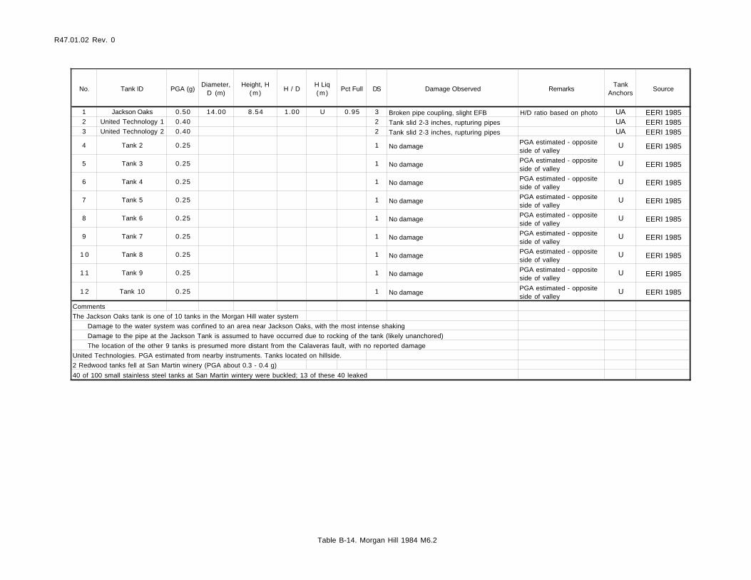
R47.01.02 Rev. 0


D (m)Height, H

(m)H / D

H Liq (m)


AnchorsSource

1 Jackson Oaks 0.50 14.00 8.54 1.00 U 0.95 3 Broken pipe coupling, slight EFB H/D ratio based on photo UA EERI 19852 United Technology 1 0.40 2 Tank slid 2-3 inches, rupturing pipes UA EERI 19853 United Technology 2 0.40 2 Tank slid 2-3 inches, rupturing pipes UA EERI 1985

4 Tank 2 0.25 1 No damagePGA estimated - opposite side of valley

U EERI 1985


U EERI 1985


U EERI 1985


U EERI 1985


U EERI 1985


U EERI 1985

1 0 Tank 8 0.25 1 No damagePGA estimated - opposite side of valley

U EERI 1985


U EERI 1985


U EERI 1985

Comments

The Jackson Oaks tank is one of 10 tanks in the Morgan Hill water system

Damage to the water system was confined to an area near Jackson Oaks, with the most intense shaking

Damage to the pipe at the Jackson Tank is assumed to have occurred due to rocking of the tank (likely unanchored)

The location of the other 9 tanks is presumed more distant from the Calaveras fault, with no reported damage

United Technologies. PGA estimated from nearby instruments. Tanks located on hillside.

2 Redwood tanks fell at San Martin winery (PGA about 0.3 - 0.4 g)

40 of 100 small stainless steel tanks at San Martin wintery were buckled; 13 of these 40 leaked

Table B-14. Morgan Hill 1984 M6.2

r47.01.02 Rev. 0



H Liq (m)


AnchorsSource

1 Richmond 1 0.13 18.85 15.10 0.80 7.55 0.50 3 Elephant foot buckling, pipe supports pulled from tank shell Tanks assumed 50% full, average dimensions U Cooper 19972 Richmond 2 0.13 18.85 15.10 0.80 7.55 0.50 3 Elephant foot buckling, pipe supports pulled from tank shell Tanks assumed 50% full, average dimensions U Cooper 19973 Richmond 3 0.13 18.85 15.10 0.80 7.55 0.50 3 Elephant foot buckling, pipe supports pulled from tank shell Tanks assumed 50% full, average dimensions U Cooper 19974 Richmond 4 0.13 18.85 15.10 0.80 7.55 0.50 3 Elephant foot buckling, pipe supports pulled from tank shell Tanks assumed 50% full, average dimensions U Cooper 19975 Richmond 5 0.13 18.85 15.10 0.80 7.55 0.50 3 Elephant foot buckling, pipe supports pulled from tank shell Tanks assumed 50% full, average dimensions U Cooper 19976 Richmond 6 0.13 18.85 15.10 0.80 7.55 0.50 2 Pipe supports pulled from tank shell Tanks assumed 50% full, average dimensions U Cooper 19977 Richmond 7 0.13 18.85 15.10 0.80 7.55 0.50 2 Pipe supports pulled from tank shell Tanks assumed 50% full, average dimensions U Cooper 19978 Richmond 8 0.13 18.85 15.10 0.80 7.55 0.50 2 Pipe supports pulled from tank shell Tanks assumed 50% full, average dimensions U Cooper 19979 Richmond 9 0.13 18.85 15.10 0.80 7.55 0.50 2 Pipe supports pulled from tank shell Tanks assumed 50% full, average dimensions U Cooper 1997

10 Richmond 10 0.13 18.85 15.10 0.80 7.55 0.50 2 Pipe supports pulled from tank shell Tanks assumed 50% full, average dimensions U Cooper 199711 Richmond 11 0.13 18.85 15.10 0.80 7.55 0.50 2 Pipe supports pulled from tank shell Tanks assumed 50% full, average dimensions U Cooper 199712 Richmond 12 0.13 18.85 15.10 0.80 7.55 0.50 2 Pipe supports pulled from tank shell Tanks assumed 50% full, average dimensions U Cooper 199713 Richmond 13 0.13 18.85 15.10 0.80 7.55 0.50 2 Pipe supports pulled from tank shell Tanks assumed 50% full, average dimensions U Cooper 199714 Richmond 14 0.13 18.85 15.10 0.80 7.55 0.50 2 Pipe supports pulled from tank shell Tanks assumed 50% full, average dimensions U Cooper 199715 Richmond 15 0.13 18.85 15.10 0.80 7.55 0.50 2 Pipe supports pulled from tank shell Tanks assumed 50% full, average dimensions U Cooper 199716 Richmond 16 0.13 18.85 15.10 0.80 7.55 0.50 2 Pipe supports pulled from tank shell Tanks assumed 50% full, average dimensions U Cooper 199717 Richmond 17 0.13 18.85 15.10 0.80 7.55 0.50 2 Pipe supports pulled from tank shell Tanks assumed 50% full, average dimensions U Cooper 199718 Richmond 18 0.13 13.00 12.00 0.92 6.00 0.50 3 Elephant foot buckling Tanks assumed 50% full, average dimensions U Cooper 199719 Richmond 19 0.13 13.00 12.00 0.92 6.00 0.50 3 Elephant foot buckling (incipient) Tanks assumed 50% full, average dimensions U Cooper 199720 Richmond 20 0.13 13.00 12.00 0.92 6.00 0.50 1 No apparent damage Tanks assumed 50% full, average dimensions U Cooper 199721 Lube 1 of 60 0.13 3.70 7.4 2.00 1.85 0.25 1 No apparent damage UA Cooper 199722 Lube 2 of 60 0.13 3.70 7.4 2.00 1.85 0.25 1 No apparent damage UA Cooper 199723 Lube 3 of 60 0.13 3.70 7.4 2.00 1.85 0.25 1 No apparent damage UA Cooper 199724 Lube 4 of 60 0.13 3.70 7.4 2.00 1.85 0.25 1 No apparent damage UA Cooper 199725 Lube 5 of 60 0.13 3.70 7.4 2.00 1.85 0.25 1 No apparent damage UA Cooper 199726 Lube 6 of 60 0.13 3.70 7.4 2.00 1.85 0.25 1 No apparent damage UA Cooper 199727 Lube 7 of 60 0.13 3.70 7.4 2.00 1.85 0.25 1 No apparent damage UA Cooper 199728 Lube 8 of 60 0.13 3.70 7.4 2.00 1.85 0.25 1 No apparent damage UA Cooper 199729 Lube 9 of 60 0.13 3.70 7.4 2.00 1.85 0.25 1 No apparent damage UA Cooper 199730 Lube 10 of 60 0.13 3.70 7.4 2.00 1.85 0.25 1 No apparent damage UA Cooper 199731 Lube 11 of 60 0.13 3.70 7.4 2.00 1.85 0.25 1 No apparent damage UA Cooper 199732 Lube 12 of 60 0.13 3.70 7.4 2.00 1.85 0.25 1 No apparent damage UA Cooper 199733 Lube 13 of 60 0.13 3.70 15.4 4.16 3.85 0.25 2 Anchor bolts restraining and bending bottom plate A Cooper 199734 Lube 14 of 60 0.13 3.70 15.4 4.16 3.85 0.25 2 Anchor bolts restraining and bending bottom plate A Cooper 199735 Lube 15 of 60 0.13 3.70 15.4 4.16 3.85 0.25 1 No apparent damage UA Cooper 199736 Lube 16 of 60 0.13 3.70 15.4 4.16 3.85 0.25 1 No apparent damage UA Cooper 199737 Lube 17 of 60 0.13 3.70 15.4 4.16 3.85 0.25 1 No apparent damage UA Cooper 199738 Lube 18 of 60 0.13 3.70 15.4 4.16 3.85 0.25 1 No apparent damage UA Cooper 199739 Lube 19 of 60 0.13 3.70 15.4 4.16 3.85 0.25 1 No apparent damage UA Cooper 199740 Lube 20 of 60 0.13 3.70 15.4 4.16 3.85 0.25 1 No apparent damage UA Cooper 199741 Lube 21 of 60 0.13 3.70 15.4 4.16 3.85 0.25 1 No apparent damage UA Cooper 199742 Lube 22 of 60 0.13 3.70 15.4 4.16 3.85 0.25 1 No apparent damage UA Cooper 199743 Lube 23 of 60 0.13 3.70 15.4 4.16 3.85 0.25 1 No apparent damage UA Cooper 199744 Lube 24 of 60 0.13 3.70 15.4 4.16 3.85 0.25 1 No apparent damage UA Cooper 199745 Lube 25 of 60 0.13 3.70 11 2.97 2.75 0.25 1 No apparent damage UA Cooper 199746 Lube 26 of 60 0.13 3.70 11 2.97 2.75 0.25 1 No apparent damage UA Cooper 199747 Lube 27 of 60 0.13 3.70 11 2.97 2.75 0.25 1 No apparent damage UA Cooper 199748 Lube 28 of 60 0.13 3.70 11 2.97 2.75 0.25 1 No apparent damage UA Cooper 199749 Lube 29 of 60 0.13 3.70 11 2.97 2.75 0.25 1 No apparent damage UA Cooper 199750 Lube 30 of 60 0.13 3.70 11 2.97 2.75 0.25 1 No apparent damage UA Cooper 199751 Lube 31 of 60 0.13 3.70 11 2.97 2.75 0.25 1 No apparent damage UA Cooper 199752 Lube 32 of 60 0.13 3.70 11 2.97 2.75 0.25 1 No apparent damage UA Cooper 199753 Lube 33 of 60 0.13 3.70 11 2.97 2.75 0.25 1 No apparent damage UA Cooper 199754 Lube 34 of 60 0.13 3.70 11 2.97 2.75 0.25 1 No apparent damage UA Cooper 199755 Lube 35 of 60 0.13 3.70 11 2.97 2.75 0.25 1 No apparent damage UA Cooper 199756 Lube 36 of 60 0.13 3.70 11 2.97 2.75 0.25 1 No apparent damage UA Cooper 199757 Lube 37 of 60 0.13 6.50 12.3 1.89 3.08 0.25 1 No apparent damage UA Cooper 199758 Lube 38 of 60 0.13 6.50 12.3 1.89 3.08 0.25 1 No apparent damage UA Cooper 199759 Lube 39 of 60 0.13 6.50 12.3 1.89 3.08 0.25 1 No apparent damage UA Cooper 1997

Table B-15. Loma Prieta 1989 M7, (Page 1 of 3)

r47.01.02 Rev. 0



H Liq (m)


AnchorsSource

60 Lube 40 of 60 0.13 6.50 12.3 1.89 3.08 0.25 1 No apparent damage UA Cooper 199761 Lube 41 of 60 0.13 6.50 12.3 1.89 3.08 0.25 1 No apparent damage UA Cooper 199762 Lube 42 of 60 0.13 6.50 12.3 1.89 3.08 0.25 1 No apparent damage UA Cooper 199763 Lube 43 of 60 0.13 6.50 12.3 1.89 3.08 0.25 1 No apparent damage UA Cooper 199764 Lube 44 of 60 0.13 6.50 12.3 1.89 3.08 0.25 1 No apparent damage UA Cooper 199765 Lube 45 of 60 0.13 6.50 12.3 1.89 3.08 0.25 1 No apparent damage UA Cooper 199766 Lube 46 of 60 0.13 6.50 12.3 1.89 3.08 0.25 1 No apparent damage UA Cooper 199767 Lube 47 of 60 0.13 6.50 12.3 1.89 3.08 0.25 1 No apparent damage UA Cooper 199768 Lube 48 of 60 0.13 6.50 12.3 1.89 3.08 0.25 1 No apparent damage UA Cooper 199769 Lube 49 of 60 0.13 9.20 12.3 1.34 3.08 0.25 1 No apparent damage UA Cooper 199770 Lube 50 of 60 0.13 9.20 12.3 1.34 3.08 0.25 1 No apparent damage UA Cooper 199771 Lube 51 of 60 0.13 9.20 12.3 1.34 3.08 0.25 1 No apparent damage UA Cooper 199772 Lube 52 of 60 0.13 9.20 12.3 1.34 3.08 0.25 1 No apparent damage UA Cooper 199773 Lube 53 of 60 0.13 9.20 12.3 1.34 3.08 0.25 1 No apparent damage UA Cooper 199774 Lube 54 of 60 0.13 9.20 12.3 1.34 3.08 0.25 1 No apparent damage UA Cooper 199775 Lube 55 of 60 0.13 9.20 12.3 1.34 3.08 0.25 1 No apparent damage UA Cooper 199776 Lube 56 of 60 0.13 9.20 12.3 1.34 3.08 0.25 1 No apparent damage UA Cooper 199777 Lube 57 of 60 0.13 9.20 12.3 1.34 3.08 0.25 1 No apparent damage UA Cooper 199778 Lube 58 of 60 0.13 9.20 12.3 1.34 3.08 0.25 1 No apparent damage UA Cooper 199779 Lube 59 of 60 0.13 9.20 12.3 1.34 3.08 0.25 1 No apparent damage UA Cooper 1997

80 Lube 60 of 60 0.13 9.20 12.3 1.34 12.3 1.00 3 Elephant foot buckling. Walkway between this tank and another pulled loose and fell to ground

UA Cooper 1997

81 San Jose 1 of 32 0.17 23.7 14.8 0.62 14.06 0.95 2 Severe bending and buckling of internal pan Assumed nearly full U Cooper 199782 San Jose 2 of 32 0.17 27 14.6 0.54 14.06 0.96 2 Severe bending and buckling of internal pan Assumed nearly full U Cooper 199783 San Jose 3 of 32 0.17 19.8 14.6 0.74 U 1 No apparent damage U Cooper 199784 San Jose 4 of 32 0.17 19.8 14.6 0.74 U 1 No apparent damage U Cooper 199785 San Jose 5 of 32 0.17 19.8 14.6 0.74 U 1 No apparent damage U Cooper 199786 San Jose 6 of 32 0.17 19.8 14.6 0.74 U 1 No apparent damage U Cooper 199787 San Jose 7 of 32 0.17 19.8 14.6 0.74 U 1 No apparent damage U Cooper 199788 San Jose 8 of 32 0.17 19.8 14.6 0.74 U 1 No apparent damage U Cooper 199789 San Jose 9 of 32 0.17 19.8 14.6 0.74 U 1 No apparent damage U Cooper 199790 San Jose 10 of 32 0.17 19.8 14.6 0.74 U 1 No apparent damage U Cooper 199791 San Jose 11 of 32 0.17 19.8 14.6 0.74 U 1 No apparent damage U Cooper 199792 San Jose 12 of 32 0.17 19.8 14.6 0.74 U 1 No apparent damage U Cooper 199793 San Jose 13 of 32 0.17 19.8 14.6 0.74 U 1 No apparent damage U Cooper 199794 San Jose 14 of 32 0.17 19.8 14.6 0.74 U 1 No apparent damage U Cooper 199795 San Jose 15 of 32 0.17 19.8 14.6 0.74 U 1 No apparent damage U Cooper 199796 San Jose 16 of 32 0.17 19.8 14.6 0.74 U 1 No apparent damage U Cooper 199797 San Jose 17 of 32 0.17 19.8 14.6 0.74 U 1 No apparent damage U Cooper 199798 San Jose 18 of 32 0.17 19.8 14.6 0.74 U 1 No apparent damage U Cooper 199799 San Jose 19 of 32 0.17 19.8 14.6 0.74 U 1 No apparent damage U Cooper 1997

100 San Jose 20 of 32 0.17 19.8 14.6 0.74 U 1 No apparent damage U Cooper 1997101 San Jose 21 of 32 0.17 19.8 14.6 0.74 U 1 No apparent damage U Cooper 1997102 San Jose 22 of 32 0.17 19.8 14.6 0.74 U 1 No apparent damage U Cooper 1997103 San Jose 23 of 32 0.17 19.8 14.6 0.74 U 1 No apparent damage U Cooper 1997104 San Jose 24 of 32 0.17 19.8 14.6 0.74 U 1 No apparent damage U Cooper 1997105 San Jose 25 of 32 0.17 19.8 14.6 0.74 U 1 No apparent damage U Cooper 1997106 San Jose 26 of 32 0.17 19.8 14.6 0.74 U 1 No apparent damage U Cooper 1997107 San Jose 27 of 32 0.17 19.8 14.6 0.74 U 1 No apparent damage U Cooper 1997108 San Jose 28 of 32 0.17 19.8 14.6 0.74 U 1 No apparent damage U Cooper 1997109 San Jose 29 of 32 0.17 19.8 14.6 0.74 U 1 No apparent damage U Cooper 1997110 San Jose 30 of 32 0.17 19.8 14.6 0.74 U 1 No apparent damage U Cooper 1997111 San Jose 31 of 32 0.17 19.8 14.6 0.74 U 1 No apparent damage U Cooper 1997112 San Jose 32 of 32 0.17 19.8 14.6 0.74 U 1 No apparent damage U Cooper 1997113 Brisbane 1 of 17 0.11 19.8 13.5 0.68 U 1 No apparent damage U Cooper 1997114 Brisbane 2 of 17 0.11 19.8 13.5 0.68 U 1 No apparent damage U Cooper 1997115 Brisbane 3 of 17 0.11 19.8 13.5 0.68 U 1 No apparent damage U Cooper 1997116 Brisbane 4 of 17 0.11 19.8 13.5 0.68 U 1 No apparent damage U Cooper 1997117 Brisbane 5 of 17 0.11 19.8 13.5 0.68 U 1 No apparent damage U Cooper 1997


r47.01.02 Rev. 0



H Liq (m)


AnchorsSource

118 Brisbane 6 of 17 0.11 19.8 13.5 0.68 U 1 No apparent damage U Cooper 1997119 Brisbane 7 of 17 0.11 19.8 13.5 0.68 U 1 No apparent damage U Cooper 1997120 Brisbane 8 of 17 0.11 19.8 13.5 0.68 U 1 No apparent damage U Cooper 1997121 Brisbane 9 of 17 0.11 19.8 13.5 0.68 U 1 No apparent damage U Cooper 1997122 Brisbane 10 of 17 0.11 19.8 13.5 0.68 U 1 No apparent damage U Cooper 1997123 Brisbane 11 of 17 0.11 19.8 13.5 0.68 U 1 No apparent damage U Cooper 1997124 Brisbane 12 of 17 0.11 19.8 13.5 0.68 U 1 No apparent damage U Cooper 1997125 Brisbane 13 of 17 0.11 19.8 13.5 0.68 U 1 No apparent damage U Cooper 1997126 Brisbane 14 of 17 0.11 19.8 13.5 0.68 U 1 No apparent damage U Cooper 1997127 Brisbane 15 of 17 0.11 19.8 13.5 0.68 U 1 No apparent damage U Cooper 1997128 Brisbane 16 of 17 0.11 19.8 13.5 0.68 U 1 No apparent damage U Cooper 1997129 Brisbane 17 of 17 0.11 19.8 13.5 0.68 U 1 No apparent damage U Cooper 1997130 Gilroy 1 0.50 24.4 8 0.33 U 0.95 1 No apparent damage Water tank assumed nearly full Cooper 1997

131 PG&E Moss Landing 1 0.24 17 12.2 0.72 U 0.9 4 Failed at floor / shell connection. Junction possibly corroded. Tank drained rapidly. Top shell course buckled

Tank assumed mostly full. Pga based on attenuation

UA Cooper 1997, USGS 1998

132 PG&E Moss Landing Distilled 1

0.24 17 12.2 0.72 U 0.9 2 failure of pipe couplings dimensions assumed. PGA based on attenuation U Cooper 1997, USGS 1998

133 PG&E Moss Landing Distilled 2

0.24 17 12.2 0.72 U 0.9 2 failure of pipe couplings dimensions assumed, PGA based on attenuation U Cooper 1997, USGS 1998

134 Los Gatos SJ 1 0.28 U U U U 0.95 4 Elephant foot buckling Bolted water tank, 1966 UA Cooper 1997, USGS 1998135 Los Gatos SJ 2 0.28 U U U U 0.95 4 IO pipe underneath tank separated from floor plate 700,00 gal tank welded steel Cooper 1997, USGS 1998136 Watsonville 1 0.54 U U U U 0.95 3 Buckled at roof / shell, no leak 1,000,000 gal tank Cooper 1997137 Watsonville 2 0.54 U U U U 0.95 1 No damage 600,000 gal tank, AWWA D100 Cooper 1997

138 Santa Cruz 1/ Scotts Valley

0.47 U U U U 0.95 2 Roof damage. Wood roof. Tanks drained due to broken inlet/outlet pipes

750,000 gal UA Cooper 1997, USGS 1998

139 Santa Cruz 2 / Scotts Valley

0.47 U U U U 0.95 2 Roof damage. Wood roof. Tanks drained due to broken inlet/outlet pipes

400,000 gal UA Cooper 1997, USGS 1998

140 Santa Cruz 3 0.47 U U U U 0.95 1 No damage 1,250,000 gal, AWWA D100 1983 Cooper 1997141 Hollister 0.1 0.95 1 No damage Built in 1960s. Pga based on attenuation USGS 1998

Comments

Richmond. Gasoline, diesel, turbine fuel, heavy fuel oil. Actual tank dimensions vary from 34 m Dx 14.8m H to 3.7m D x 15.4m H

Richmond tanks use cone roofs, CIP, F roof systems. Site is marine area with possibly poor soils. All tanks on pile foundations with pile caps

Richmond. No apparent roof damage at this site

Lube 1 to 60. Most tanks assumed 25% full (from report which states "less than half full" )

San Jose. Actual tank dimensions vary from 38 m D x 14.6 m H to 7.5 m D x 9.8 m H. Initial construction of these tanks was in 1965

Brisbane. Located firm ground, hillside location (assumed rock). All tanks have C, F or CF roofs; all tanks built before seismic codes. No damage

PG&E Moss Landing. DS set to 4, reflecting buckling of top shell, tearing of bottom course and loss of contents". Other tanks at this site had no damage. PGA = 0.24g based on attenuation.

Several other tanks at this site (include 2 MG oil tank) did not have major damage. PGA = 0.39g suggested in EERI (1990 p210) based on a recording located 15 km away

The EBMUD water utility operated about 50 water steel tanks at the time of the earthquake. All were shaken with ground motions between PGA = 0.03g and PGA = 0.10g. Most of

these tanks were anchored and designed per AWWA with seismic provisions. The only reported damage was 2 tanks with internal roof damage (There were no specific seismic designs of the roof systems)

All these tanks are located on rock with concrete ring foundations. About half have wood roofs and half have integral steel roofs

Most of the tanks were welded steel; a few were either riveted or bolted steel

Most of the tanks use bottom entering inlet / outlet pipes. No pipe damage was noted for any tank

Not all tanks have been inspected for internal damage to roof systems, so some unknown damage to roof systems may have occurred

San Lorenzo. Near epicentral region. 5 redwood tanks were lost (10,000 to 15,000 gallons each)

Santa Cruz mountains (in epicentral region). Several small bolted steel tanks failed, broken inlet / outlet pipes, some tanks collapsed [USGS 1998]

Watsonville. 8 other water storage facilities performed well (unknown types)

Richmond - Hercules - Rodeo - Martinez - Benicia - Avon locations include about 1,700 flat bottom steel tanks. PGA ranges from about 0.03g (rock outcrop sites) to at most 0.13-0.15g (soft soil sites)

This report covers only 80 of these 1,700 tanks. All damage to tanks were for tanks at soft soil sites, and nearly full tanks


R47.01.02 Rev. 0


D (m)Height, H

(m)H / D

H Liq (m)


AnchorsSource

1 701 0.35 44.21 9.76 0.22 9.12 0.93 2 Roof damage, fire caused by tank 792 Welded steel UA Ballantyne and Crouse 19972 704 0.35 44.21 12.20 0.28 11.52 0.95 2 Roof damage Welded steel UA Ballantyne and Crouse 19973 705 0.35 44.21 12.20 0.28 11.52 0.95 2 Roof damage Welded steel UA Ballantyne and Crouse 19974 708 0.35 21.16 9.76 0.46 9.30 0.95 3 Elephant foot buckling Welded steel UA Ballantyne and Crouse 19975 709 0.35 21.16 9.76 0.46 9.30 0.95 3 Elephant foot buckling Welded steel UA Ballantyne and Crouse 19976 715 0.35 29.70 12.20 0.41 11.49 0.94 2 Roof damage Welded steel UA Ballantyne and Crouse 19977 717 0.35 17.87 11.43 0.64 11.28 0.99 2 Roof damage Welded steel UA Ballantyne and Crouse 19978 725 0.35 17.87 11.43 0.64 11.28 0.99 2 Roof damage Welded steel UA Ballantyne and Crouse 19979 726 0.35 17.87 11.43 0.64 11.28 0.99 2 Roof damage, tank lateral movement Welded steel UA Ballantyne and Crouse 1997

1 0 728 0.35 40.85 12.20 0.30 11.77 0.97 3 Shell buckling near roof, tank lateral movement

Welded steel UA Ballantyne and Crouse 1997

1 1 Unknown 0.35 40.85 12.20 0.30 11.43 0.94 2 Tank lateral movement Welded steel UA Ballantyne and Crouse 1997

1 2 738 0.35 14.63 9.76 0.67 9.48 0.97 4 Elephant foot bucklingWelded steel. See note below about assumed EFB failure

UA Ballantyne and Crouse 1997

1 3 745 0.35 10.37 9.76 0.94 9.45 0.97 3 Elephant foot buckling Welded steel UA Ballantyne and Crouse 19971 4 792 0.35 4.79 4.85 1.01 4.85 1.00 5 Overturned tank, explosion Welded steel UA Ballantyne and Crouse 19971 5 Holanda Chem Plant 0.35 5.53 5.53 1.00 3 Slight Elephant foot buckle New API 650 tank UA Spectra, Vol 7, B, 19911 6 Holanda Chem Plant 0.35 10.06 10.06 1.00 2 Slid 20 cm UA Spectra, Vol 7, B, 19911 7 Holanda Chem Plant 0.35 1 No damage UA Spectra, Vol 7, B, 19911 8 Holanda Chem Plant 0.35 1 No damage UA Spectra, Vol 7, B, 19911 9 Holanda Chem Plant 0.35 1 No damage UA Spectra, Vol 7, B, 19912 0 Holanda Chem Plant 0.35 1 No damage UA Spectra, Vol 7, B, 19912 1 Holanda Chem Plant 0.35 1 No damage UA Spectra, Vol 7, B, 19912 2 Holanda Chem Plant 0.35 1 No damage UA Spectra, Vol 7, B, 19912 3 Holanda Chem Plant 0.35 1 No damage UA Spectra, Vol 7, B, 19912 4 Holanda Chem Plant 0.35 1 No damage UA Spectra, Vol 7, B, 19912 5 Holanda Chem Plant 0.35 1 No damage UA Spectra, Vol 7, B, 19912 6 Holanda Chem Plant 0.35 1 No damage UA Spectra, Vol 7, B, 19912 7 Transmerquim 0.35 8.66 8.66 3 EFB - severe, no leak Built 1989 UA Spectra, Vol 7, B, 19912 8 Transmerquim 0.35 8.66 8.66 3 EFB - severe, no leak Built 1989 UA Spectra, Vol 7, B, 1991

2 9 Transmerquim 0.35 2 Rocking, broken inlent/outlet pipe, loss of some contents

UA Spectra, Vol 7, B, 1991

3 0 Transmerquim 0.35 1 No damage UA Spectra, Vol 7, B, 19913 1 Transmerquim 0.35 1 No damage UA Spectra, Vol 7, B, 19913 2 Transmerquim 0.35 1 No damage UA Spectra, Vol 7, B, 19913 3 Transmerquim 0.35 1 No damage UA Spectra, Vol 7, B, 19913 4 Transmerquim 0.35 1 No damage UA Spectra, Vol 7, B, 19913 5 Transmerquim 0.35 1 No damage UA Spectra, Vol 7, B, 19913 6 Transmerquim 0.35 1 No damage UA Spectra, Vol 7, B, 19913 7 Transmerquim 0.35 1 No damage UA Spectra, Vol 7, B, 19913 8 Transmerquim 0.35 1 No damage UA Spectra, Vol 7, B, 1991

Comments

Tanks 1 - 14 at Recope Refinery, Port of Moin, Costa Rica

Spillage of oil from at least one tank was confined in a dike. This is arbitrarily assigned to tank 738 (DS=4)

Holanda Chemical Plant. 2 of 12 tanks were damaged

Transmerquim plant located next to Holanda. 2 of 12 tanks suffered EFB

The level of ground shaking at these three sites was considered "moderate" but not instrumental recordings available

Ground motion for Port of Moin, near Limon, was estimated based on mapped intensity MMI VIII = PGA 0.35g.

Table B-16. Costa Rica 1991 M7.5

R47.01.02 Rev. 0


D (m)Height, H

(m)H / D

H Liq (m)


AnchorsSource

1 BDVWA A 0.56 16.90 7.30 0.43 6.68 0.92 4

EFP around entire tank, failed at shell / bottom plate at 2 locations. 6" overflow pipe failed, lifted 2 feet out of ground. Tank shifted 3" laterally. Failure of side pipe

Welded steel, AWWA D100 1974, 0.25: shell, 0.25" bottom, 3/16" roof

UA Cooper 1997, Ballantyne and Crouse 1997

2 BDVWA B 0.55 8.10 7.30 0.90 6.95 0.95 2 Minor damage UA Cooper 1997, Ballantyne and Crouse 19973 BDVWA C 0.55 18.10 7.30 0.40 6.89 0.94 2 Minor damage UA Cooper 1997, Ballantyne and Crouse 19974 BDVWA 10 0.55 9.90 4.90 0.49 4.45 0.91 2 Minor damage UA Cooper 1997, Ballantyne and Crouse 19975 BDVWA 22-A 0.54 9.90 4.90 0.49 4.45 0.91 2 Minor damage UA Cooper 1997, Ballantyne and Crouse 19976 BDVWA 22-B 0.54 9.90 4.90 0.49 4.45 0.91 2 Minor damage UA Cooper 1997, Ballantyne and Crouse 19977 BDVWA 22-C 0.54 14.00 4.90 0.35 4.45 0.91 2 Minor damage UA Cooper 1997, Ballantyne and Crouse 19978 BDVWA 22-D 0.54 22.30 4.90 0.22 4.42 0.90 2 Minor damage UA Cooper 1997, Ballantyne and Crouse 19979 BDVWA 34 0.55 6.40 4.90 0.77 4.48 0.91 2 Minor damage UA Cooper 1997, Ballantyne and Crouse 1997

1 0 HDWD 2 M.G. 0.15 36.60 7.30 0.20 U 1 No significant damage UA Cooper 1997, Wald 19981 1 HDWD R-7 0.15 25.90 7.30 0.28 U 1 No significant damage UA Cooper 1997, Wald 19981 2 HDWD R-8 0.15 10.00 7.30 0.73 U 1 No significant damage UA Cooper 1997, Wald 19981 3 HDWD R-14 0.20 21.30 5.50 0.26 U 1 No significant damage UA Cooper 1997, Wald 19981 4 HDWD R-15 0.19 22.90 7.30 0.32 U 1 No significant damage UA Cooper 1997, Wald 19981 5 HDWD R-2 0.15 25.90 7.30 0.28 U 1 No significant damage UA Cooper 1997, Wald 19981 6 HDWD R-3 0.20 25.90 7.30 0.28 U 1 No significant damage UA Cooper 1997, Wald 19981 7 HDWD R-4 0.20 9.10 7.30 0.80 U 1 No significant damage UA Cooper 1997, Wald 19981 8 HDWD R-5 0.20 7.90 7.30 0.92 U 1 No significant damage UA Cooper 1997, Wald 19981 9 HDWD Upper Ridge 0.10 13.10 7.30 0.56 U 1 No significant damage UA Cooper 1997, Wald 19982 0 HDWD Lower Ridge 0.10 5.50 4.9 0.89 U 1 No significant damage UA Cooper 1997, Wald 19982 1 HDWD Upper Fox 0.15 24.40 12.2 0.50 U 1 No significant damage UA Cooper 1997, Wald 19982 2 HDWD Lower Fox 0.15 10.90 4.9 0.45 U 1 No significant damage UA Cooper 1997, Wald 19982 3 HDWD Golden Bee 0.15 14.40 9.8 0.68 U 1 No significant damage UA Cooper 1997, Wald 19982 4 HDWD Homestead 0.10 11.80 7.3 0.62 U 1 No significant damage UA Cooper 1997, Wald 1998

2 5 HDWD Hospital Desert Gold

0.15 11.8 7.3 0.62 U 1 No significant damage UA Cooper 1997, Wald 1998

2 6 CSA 70-1 0.47 11.8 7.3 0.62 6.71 0.92 4 EFB all around, shell tearing, pullout of dresser couplings for 2 side attached pipes

Designed per API 12B, 1979, Bolted steel, 10 ga shell 10ga bottom plate

UA Cooper 1997, Wald 1998

2 7 Beryl - SCWC 0.14 9.14 7.32 0.80 6.4 0.87 2 Small Leakage of bottom flange Bolted U Ballantune and Crouse 19972 8 Basalt - SCWC 0.14 9.14 7.32 0.80 6.4 0.87 2 Failure of pipe through bottom penetration Bolted U Ballantune and Crouse 19972 9 Arville-N - SCWC 0.14 8.93 12.65 1.42 11.28 0.89 2 Failure of pipe through bottom penetration Welded (fillet) U Ballantune and Crouse 19973 0 Arville-S - SCWC 0.14 8.93 13.56 1.52 12.19 0.90 1 tank lateral movement Welded U Ballantune and Crouse 19973 1 SCE Coolwater 1 of 3 0.53 83.2 15.2 0.18 15.2 1.00 1 No damage API 650 U Cooper 19973 2 SCE Coolwater 2 of 3 0.53 83.2 15.2 0.18 13.68 0.90 1 No damage API 650 U Cooper 19973 3 SCE Coolwater 3 of 3 0.53 67.2 14.5 0.22 1.45 0.10 1 No damage API 650 U Cooper 1997

Comments

Landers Mw 7.3 followed by Big Bear M 6.5 3 hours later

All damage in this table due to Landers event

BDVWA = Bighorn Desert View Water Agency. HDWD = Hi Desert Water District. CSA = San Bernardino County Service Area 70

SCWC - 4 tanks in Barstow, CA

Table B-17. Landers 1992 M7.3

R47.01.02 Rev. 0


D (m)Height, H

(m)H / D

H Liq (m)


AnchorsSource

1 Van Nuys 1 0.55 8.80 14.60 1.66 7.90 0.54 1 Bolt shearing on tank walkwayAssumed between 1/3 and 2/3 full. API 650 1963 UA Cooper 1997, Wald 1998





6 1 of 5 0.55 3.20 10.00 3.13 9.50 0.95 1 Minor damage to walkway Assumed nearly full UA Cooper 1997, Wald 19987 2 of 5 0.55 3.20 10.00 3.13 9.50 0.95 1 Minor damage to walkway Assumed nearly full UA Cooper 1997, Wald 19988 3 of 5 0.55 3.20 10.00 3.13 0.00 0.00 1 Minor damage to walkway Assumed nearly full UA Cooper 1997, Wald 19989 4 of 5 0.55 3.20 10.00 3.13 0.00 0.00 1 Minor damage to walkway Assumed nearly full UA Cooper 1997, Wald 1998

1 0 5 of 5 0.55 3.20 10.00 3.13 0.00 0.00 1 No significant damageAssumed other 3 tanks out of service had no liquid UA Cooper 1997, Wald 1998

1 1 A Sepulveda Terminal 0.90 19.80 11.00 0.56 7.32 0.67 1 Slight sloshing API 650, mid-60s UA Cooper 1997, Wald 1998, EERI 19951 2 B 0.90 21.90 11.00 0.50 3.66 0.33 1 Slight sloshing API 650, mid-60s UA Cooper 1997, Wald 1998, EERI 19951 3 C 0.90 18.30 11.00 0.60 3.66 0.33 1 Slight sloshing API 650, mid-60s UA Cooper 1997, Wald 1998, EERI 19951 4 AG 1 0.90 3.70 7.30 1.97 7.30 1.00 1 Minor paint cracks UL 142, mid-60s A Cooper 1997, Wald 19981 5 AG 2 0.90 3.70 7.30 1.97 0.00 0.00 1 No significant damage UL 142, mid-60s A Cooper 1997, Wald 1998

1 6 Aliso 1 0.70 12.20 7.30 0.60 U 0.75 5 CollapseBolted, mostly full based on amount of leakage U Cooper 1997, Wald 1998

1 7 Aliso 2 0.70 12.20 7.30 0.60 U 3 Photo shows some shell damage Bolted, may be damaged U Cooper 1997, Wald 19981 8 Aliso 3 0.70 12.20 7.30 0.60 U 1 No significant damage Bolted U Cooper 1997, Wald 19981 9 Aliso 4 0.70 12.20 7.30 0.60 U 1 No significant damage Bolted U Cooper 1997, Wald 19982 0 Amir 0.90 12.80 9.09 0.71 U 3 EFB U Ballantyne and Crouse 1997, Wald 1998

2 1 Lautenschlager 1 0.90 19.00 6.7 0.35 5.94 0.89 1 No significant damage Welded, 1965 UCooper 1997, Ballantyne and Crouse 1997

Wald 1998

2 2 Lautenschlager 2 0.90 19.00 7.3 0.38 5.94 0.81 1 No significant damage Welded 1988 UCooper 1997, Ballantyne and Crouse 1997

Wald 1998

2 3 Tapo 0.90 40.00 9.8 0.25 8.69 0.89 1 No significant damage Welded 1963 UCooper 1997, Ballantyne and Crouse 1997

Wald 1998

2 4 Crater East 0.75 9.10 7.3 0.80 6.13 0.84 1 No significant damage Survived, pct full from text in Cooper UCooper 1997, Ballantyne and Crouse 1997

Wald 1998

2 5 Crater West 0.75 11.90 7.3 0.61 6.13 0.84 1 No significant damage Survived, pct full from text in Cooper UCooper 1997, Ballantyne and Crouse 1997

Wald 1998

2 6 Alamo 0.70 30.50 6.3 0.21 6.25 0.99 1 No significant damage Welded 1964 UCooper 1997, Ballantyne and Crouse 1997

Wald 1998

2 7 Katerine 0.90 12.00 7.3 0.61 6.25 0.86 4 Failed by EFB with loss of contents Bolted, built 1964 UCooper 1997, Ballantyne and Crouse 1997

Wald 1998

2 8 Rebecca North 0.85 12.00 7.3 0.61 6.86 0.94 4 Failed by EFB with loss of contents Bolted, built 1964 UCooper 1997, Ballantyne and Crouse 1997

Wald 1998

2 9 Rebecca South 0.85 12.00 7.3 0.61 6.86 0.94 4 Failed by EFB with loss of contents Bolted, built 1964 UCooper 1997, Ballantyne and Crouse 1997

Wald 1998

3 0 Sycamore North 0.70 9.10 7.3 0.80 5.03 0.69 4 Failed by EFB with loss of contents Bolted, built 1964 UCooper 1997, Ballantyne and Crouse 1997

Wald 1998

3 1 Sycamore South 0.70 9.10 7.3 0.80 5.03 0.69 4 Failed by EFB with loss of contents Bolted, built 1964 UCooper 1997, Ballantyne and Crouse 1997

Wald 19983 2 SCWC 1 of 4 0.70 15.80 9.8 0.62 U 0.99 1 Survived Welded U Cooper 1997, Wald 1998

Table B-18. Northridge 1994 M6.7 (Page 1 of 3)

R47.01.02 Rev. 0


D (m)Height, H

(m)H / D

H Liq (m)


AnchorsSource

3 3 SCWC 2 of 4 0.70 15.80 9.8 0.62 U 1 Survived Welded U Cooper 1997, Wald 19983 4 SCWC 3 of 4 0.70 27.40 9.8 0.36 U 1 Survived Welded U Cooper 1997, Wald 19983 5 SCWC 4 of 4 0.70 39.00 9.8 0.25 U 1 Survived Welded U Cooper 1997, Wald 1998

3 6 LADWP Topanga 0.40 11.00 9 0.82 8.08 0.90 2Replaced broken inlet / outlet valve. Loss of contents

Pct full from B&C. Welded steel, built 1936 UA

Cooper 1997, Ballantyne and Crouse 1997, Brown et al 1995

3 7 LADWP Zelzah 0.50 21.30 12.2 0.57 9.85 0.81 2Roof collapsed, local buckling at top, broken valve. Loss of contents

Pct full from B&C. Welded steel built 1948 UA


3 8 LADWP Mulholland 0.40 15.80 10.2 0.65 0 0.00 2overflow pipe pulled away. Loss of contents

Pct full from B&C. Welded steel built 1931 UA


3 9 LADWP Beverly Glen 0.50 30.50 12.3 0.40 U 2

Roof collapsed, local buckling, dresser coupling pulled out. Loss of contents

Riveted, built 1932. Wood roof replaced with hypalon bladder UA Cooper 1997, Brown et al 1995

4 0 MWD Jensen Clearwell 0.70 42.67 12.19 0.29 11.67 0.96 1 No tank damage UACooper 1997, Ballantyne and Crouse

1997, Brown et al 1995

4 1 LADWP Coldwater 0.30 30.48 12.19 0.40 U 2Roof shifted and collapsed, inlet / outlet pipe failure. Loss of contents

Riveted built 1925. Wood roof shifted and collapsed. UA

Ballantyne and Crouse 1997, Brown et al 1995

4 2 LADWP Granada High 1.00 16.80 10.7 0.64 9.66 0.90 5 Tank collapsed and tank removed

Riveted built 1929. Same tank was damaged in the 1971 San Fernando EQ UA


4 3 LADWP Alta Vista 1 0.60 16.46 8.78 0.53 8.84 1.01 1 No tank damage Riveted built 1929 UACooper 1997, Ballantyne and Crouse

1997, Brown et al 1995

4 4 LADWP Alta Vista 2 0.60 28.96 11.13 0.38 9.3 0.84 1 No tank damageWelded steel, built 1954. Assumed same pga as Alta Vista 1 UA


4 5 LADWP Alta View 0.30 19.81 12.95 0.65 12.5 0.97 1 Settlement UABallantyne and Crouse 1997, Brown et al

1995

4 6 LADWP Kittridge 3 0.30 57.90 15.54 0.27 U 1 No tank damage Welded built 1973 UABallantyne and Crouse 1997, Brown et al

1995

4 7 LADWP Kittridge 4 0.30 57.90 15.54 0.27 U 1 No tank damage Welded built 1987 UABallantyne and Crouse 1997, Brown et al

1995

4 8 LADWP Corbin 0.43 47.50 9.1 0.19 7.62 0.84 2Minor drain line damage, partially buried Welded built 1987 UA


4 9 Donick 0.30 37.43 7.32 0.20 6.86 0.94 1 No tank damage UABallantyne and Crouse 1997, Brown et al

1995

5 0 Santa Clarita 0.56 24.38 12.19 0.50 11.89 0.98 4 EFB, roof damage

Assumed same PGA as Magic Mountain tanks (also located at Valencia) U

Cooper 1997, Ballantyne and Crouse 1997, Wald 1998

5 1Valencia Round

Moutain 0.56 40.30 9.8 0.24 9.07 0.93 1 No tank damage AWWA D100 UCooper 1997, Ballantyne and Crouse

1997, Wald 19985 2 Hasley 0.50 36.60 12.2 0.33 11.29 0.93 1 No tank damage AWWA D100 U Cooper 1997, Wald 1998

5 3 Magic Mountain 2 0.56 22.30 7.3 0.33 6.1 0.84 U Damaged by outflow of MM 1 Bolted, 1975 UCooper 1997, Ballantyne and Crouse

1997, Wald 1998

5 4 Magic Mountain 1 0.56 18.30 7.3 0.40 6.1 0.84 5Complete failure, bottom shell torn at base, collapse Bolted, 1971 U


5 5 Magic Mountain 3 0.56 24.40 9.8 0.40 9.07 0.93 1No damage, tank partially buried 2.5 feet

AWWA D100. Welded with external roof rafters U


5 6 Presley 0.50 21.30 9.8 0.46 9.07 0.93 1 No damage AWWA D100 U Cooper 1997, Wald 19985 7 4 Million 0.55 45.70 9.1 0.20 8.42 0.93 1 No damage AWWA D100 U Cooper 1997, Wald 19985 8 Seco 0.43 22.30 7.3 0.33 6.75 0.92 1 No damage AWWA D100 U Cooper 1997, Wald 1998


R47.01.02 Rev. 0


D (m)Height, H

(m)H / D

H Liq (m)


AnchorsSource

5 9 Larwin 0.55 18.30 12.2 0.67 9.75 0.80 5

Complete failure, EFB, tie down straps pulled, lifted foundation, nozzle tear outs

AWWA D100 1986. Straps 3/8"x3" at 4" On Center. A Cooper 1997, Wald 1998, EERI 1995

6 0 Poe 0.55 27.40 9 0.33 8.33 0.93 2Roof rafter damage, sagging roof, no EFB AWWA D100 U Cooper 1997, Wald 1998

6 1 Paragon 0.43 22.30 9.8 0.44 9.07 0.93 1 No damage AWWA D100 U Cooper 1997, Wald 1998

6 2 Newhall 1 0.63 18.29 9.14 0.50 8.23 0.90 5EFB, collapse, piping damage. Tasnk failed Welded UA Cooper 1997, Wald 1998, EERI 1995

6 3 Newhall 2 0.63 12.20 9.8 0.80 8.82 0.90 3Broken piping. EFB, Foundation settling Built 1954, welded UA Cooper 1997, Wald 1998, EERI 1995

6 4 Newhall 3 0.63 12.20 9.8 0.80 8.82 0.90 3Broken piping, EFB, Foundation settling Built 1954, welded UA Cooper 1997, Wald 1998, EERI 1995

6 5 Newhall 4 0.63 12.20 9.8 0.80 8.82 0.90 3Broken piping, EFB, Foundation settling, Roof rafters pulled out Built 1962, AWWA UA Cooper 1997, Wald 1998, EERI 1995

6 6 Newhall 5 0.63 19.50 9.8 0.50 8.82 0.90 4Roof rafter damage, EFB, inlet/outlet piping sheared Built 1962. DS changed from 3 to 4 UA Cooper 1997, Wald 1998, EERI 1995

6 7 Newhall 6 0.63 6.10 6.1 1.00 5.49 0.90 5EFB, piping failure, plate failure, Tank replaced Built 1960s UA Cooper 1997, Wald 1998, EERI 1995

6 8 Newhall 7 0.63 27.40 9.8 0.36 8.82 0.90 2Roof shell seam opened, rafters fell, no EFB Built 1975. Bottom course t=0.5" UA Cooper 1997, Wald 1998, EERI 1995

6 9 Newhall 8 0.63 18.30 7.3 0.40 6.57 0.90 2Roof rafters pulled away from the shell, roof damage UA Cooper 1997, Wald 1998

7 0 Newhall 10 0.63 24.40 12.2 0.50 10.98 0.90 1 No apparent damage Built 1989, AWWA UA Cooper 1997, Wald 1998

Comments

City of Simi Water District. 34 tanks in District, about 10 had damage. All damaged tanks were at east end of District (closer to fault). None of these tanks are in the table above

Simi: one tank had a failed underdrain pipe. Visual inspection of 2 tanks showed them unanchored, likely all were unanchored. This data not in above table

SCWC = Southern California Water Company

LADWP = Los Angeles Department of Water and Power

Tanks 51 - 61 are part of the Valencia Water Company

Tanks 62-70 are all welded, built to AWWA D100 or similar criteria

8 Prestressed concrete circular tanks in region with strong shaking (>0.2g) (6 buried or partially buried) performed well, built 1958-1992

There were other steel tanks at industrial sites which had EFB, which are not reported in this table

Tanks A, B, C, AG1, AG2 are at the Sepulveda terminal


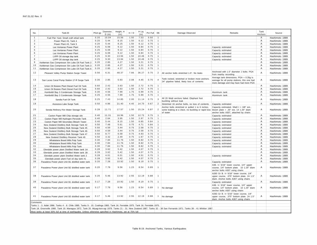
R47.01.02 Rev. 0


D (m)Height, H

(m)H / D

H Liq (m)


AnchorsSource

1 Fuel Pier Yard. Small craft refuel tank 0.20 10.04 15.06 1.50 7.53 0.50 1 A Hashimoto 19892 Power Plant #3, Tank 4 0.20 5.44 8.15 1.50 6.12 0.75 1 A Hashimoto 19893 Power Plant #3, Tank 5 0.20 5.44 8.15 1.50 6.12 0.75 1 A Hashimoto 19894 Las Ventanas Power Plant 0.25 6.08 9.12 1.50 6.84 0.75 1 Capacity estimated A Hashimoto 19895 Las Ventanas Power Plant 0.25 6.08 9.12 1.50 6.84 0.75 1 Capacity estimated A Hashimoto 19896 Las Ventanas Power Plant 0.25 6.08 9.12 1.50 6.84 0.75 1 Capacity estimated A Hashimoto 19897 LVPP Oil storage day tank 0.25 9.30 13.94 1.50 10.46 0.75 1 Capacity estimated A Hashimoto 19898 LVPP Oil storage day tank 0.25 9.30 13.94 1.50 10.46 0.75 1 Capacity estimated A Hashimoto 19899 Kettleman Gas Compressor Stn Lube Oil Fuel Tank 2 0.20 2.85 4.27 1.50 3.21 0.75 1 A Hashimoto 1989

1 0 Kettleman Gas Compressor Stn Lube Oil Fuel Tank 3 0.20 2.85 4.27 1.50 3.21 0.75 1 A Hashimoto 19891 1 Kettleman Gas Compressor Stn Lube Oil Fuel Tank 6 0.20 2.85 4.27 1.50 3.21 0.75 1 A Hashimoto 1989

1 2 Pleasant Valley Pump Station Surge Tower 0.56 6.31 48.37 7.66 36.27 0.75 2 All anchor bolts stretched 1.5". No leaksAnchroed with 1.5" diameter J bolts. PGA from nearby recording

A Hashimoto 1989

1 3 San Lucas Canal Pump Station 17-R Surge Tank 0.35 2.85 5.93 2.08 4.45 0.75 4 Tank rocked, stretched or broken most anchors. 24" pipeline failed, likely loss of contents

Average tank dimensions. PGA = 0.35g is average for all pump stations, this one had more damage and may have had more PGA

A Hashimoto 1989

1 4 Union Oil Butane Plant Diesel Fuel Oil Tank 0.60 2.42 3.63 1.50 2.72 0.75 1 A Hashimoto 19891 5 Union Oil Butane Plant Diesel Fuel Oil Tank 0.60 2.42 3.63 1.50 2.72 0.75 1 A Hashimoto 19891 6 Humboldt Bay 3 Condensate Storage Tank 0.30 4.56 7.99 1.75 5.99 0.75 1 Aluminum tank A Hashimoto 19891 7 Humboldt Bay 3 Condensate Storage Tank 0.25 4.56 7.99 1.75 5.99 0.75 1 Aluminum tank A Hashimoto 1989

1 8 Sandia Fuel Oil Tank 0.25 7.43 14.85 2.00 11.14 0.75 3 All 20 Wejit anchors failed. Elephant foot buckling without leak

A Hashimoto 1989

1 9 Asososca Lake Surge Tank 0.50 4.86 21.40 4.40 14.70 0.67 2 Stretched 16 anchor bolts, no loss of contents Capacity estimated A Hashimoto 1989

2 0 Sendai Refinery Fire Water Storage Tank 0.28 11.71 17.57 1.50 15.24 0.87 2Anchor bolts stretched or pulled 1 to 6 inches, some leaking at a vlave, no buckling or rapid loss of water

Capacity estimated. Shell t = 3/8" est., btoom plate = .25" est. 14 1.25" diam anchor bolts A307, attached by chairs

A Hashimoto 1989

2 1 Caxton Paper Mill Chip storage silo 0.40 11.31 16.96 1.50 12.72 0.75 1 Capacity estimated A Hashimoto 19892 2 Caxton Paper Mill Hydrogen Peroxide Tank 0.40 2.64 3.95 1.50 2.97 0.75 1 Capacity estimated A Hashimoto 19892 3 Caxton Paper Mill Secondary Bleach Tower 0.40 5.44 8.15 1.50 6.85 0.84 1 Capacity estimated A Hashimoto 19892 4 New Zealand Distillery Bulk Storage Tank #2 0.50 7.48 5.61 0.75 4.71 0.84 1 Capacity estimated A Hashimoto 19892 5 New Zealand Distillery Bulk Storage Tank #5 0.50 4.59 3.44 0.75 2.58 0.75 1 Capacity estimated A Hashimoto 19892 6 New Zealand Distillery Bulk Storage Tank #6 0.50 4.59 3.44 0.75 2.58 0.75 1 Capacity estimated A Hashimoto 19892 7 New Zealand Distillery Bulk Storage Tank #7 0.50 8.77 6.58 0.75 4.93 0.75 1 Capacity estimated A Hashimoto 19892 8 New Zealand Distillery Receiver Tank #9 0.50 3.32 2.49 0.75 1.87 0.75 1 Capacity estimated A Hashimoto 19892 9 Whakatane Board Mills Pulp Tank 0.30 7.84 11.76 1.50 8.82 0.75 1 Capacity estimated A Hashimoto 19893 0 Whakatane Board Mills Pulp Tank 0.30 7.84 11.76 1.50 8.82 0.75 1 Capacity estimated A Hashimoto 19893 1 Whakatane Board Mills Pulp Tank 0.30 7.84 11.76 1.50 8.82 0.75 1 Capacity estimated A Hashimoto 19893 2 Glendale power plant Distilled Water tank 1A 0.28 3.62 5.42 1.50 4.07 0.75 1 A Hashimoto 19893 3 Glendale power plant Distilled Water tank 1B 0.28 3.62 5.42 1.50 4.07 0.75 1 A Hashimoto 19893 4 Glendale power plant Distilled Water tank 2 0.28 4.01 6.01 1.50 4.51 0.75 1 Capacity estimated A Hashimoto 19893 5 Glendale power plant Fuel oil day tank #1 0.28 3.62 5.42 1.50 4.07 0.75 1 A Hashimoto 19893 6 Pasadena Power plant Unit B1 distilled water tank 0.20 7.28 10.92 1.50 8.19 0.75 1 Capacity estimated A Hashimoto 1989

3 7 Pasadena Power plant Unit B2 distilled water tank 0.20 7.78 9.56 1.23 8.54 0.89 1A36. t= 5/16" lower course, 1/4" upper course, 1/4" bottom plate. 10 1.25" diam anchor bolts A307 using chairs

A Hashimoto 1989

3 8 Pasadena Power plant Unit B3 distilled water tank 0.20 5.46 13.92 2.55 12.19 0.88 1A283 Gr B. t= 5/16" lower course, 1/4" upper course, .375" bottom plate. 24 1.5" diam. Anchor bolts A307 using chairs

A Hashimoto 1989

3 9 Pasadena Power plant Unit B1 distilled water tank 0.17 7.28 10.92 1.50 8.19 0.75 1 Capacity estimated A Hashimoto 1989

4 0 Pasadena Power plant Unit B2 distilled water tank 0.17 7.78 9.56 1.23 8.54 0.89 1 No damageA36. t= 5/16" lower course, 1/4" upper course, 1/4" bottom plate. 10 1.25" diam anchor bolts A307 using chairs

A Hashimoto 1989

4 1 Pasadena Power plant Unit B3 distilled water tank 0.17 5.46 13.92 2.55 12.19 0.88 1 No damageA283 Gr B. t= 5/16" lower course, 1/4" upper course, .375" bottom plate. 24 1.5" diam. Anchor bolts A307 using chairs

A Hashimoto 1989

Comments

Tanks 1 - 3. Adak 1986. Tanks 4 - 8. Chile 1985. Tanks 9 - 15. Coalinga 1983. Tank 16. Ferndale 1975. Tank 16. Ferndale 1975.

Tank 18. Greenville 1980. Tank 19. Managua 1972. Tank 20. Miyagi-ken-ogi 1978. Tanks 21 - 31. New Zealand 1987. Tanks 32 - 38 San Fernando 1971. Tanks 39 - 41 Whittier 1987.

Most tanks at least 50% full at time of earthquake. Unless otherwise specified in Hashimoto, set at 75% full

Table B-19. Anchored Tanks, Various Earthquakes

R47.01.02 Rev. 0

Abbreviation DescriptionA AnchoredAPI American Petroleum Institute (API 650 code)AWWA American Water Waorks Association (AWWA D100 code)D Diameter. For most tanks, the diameter dimension is the inside diameter of the tankDS Damage State. See text for descriptions. May be from 1 to 5EERI Earthquake Engineering Research InstituteEFB Elephant Foot Bucklingg acceleration of gravity (=32.2 ft / sec / sec)ga gage thickness

H Height. Generally the height from the top of the floor to the overflow level. The actual tank may be higher (above the overflow level)

I/O Inlet / outlet pipeLiq Height of Liquid. The estimated (sometimes known) height of fluid contents at the time of the earthquake

m meter. Note: most tanks in these tables are actually sized to the nearest foot. The metric conversion here does not infer accuracy to the exact dimension in feet.

MMI Modified Mercalli IntensityPct Full The percent full of the tank (= H Liq / H)PGA Peak Ground Acceleration in gU UnknownUA UnanchoredZ Design level peak ground acceleration

Table B-20. Legend for Tables B-8 Through B-19

Figure B-1. Elevation of Example Tank

6“ min. clearance

Shell manhole(typ. of 2)

75'-0" O.D. Steel Shell

76'-10" O.D. Footing Ring

32'-0"

Altitude Valve Control pipeAir VacuumRelease Pipe

Overflow pipe

Hold Down (Typ)

Overflow Elev 31'-0"

��

Appendices R47.01.02 Rev. 1. 7/12/2001


C. Commentary – TunnelsSection C.1 describes two sets of fragility curves which are in the literature: those inHAZUS, and those in ATC-13.

Sections C.2 through C.5 provide information of the performance of tunnels in pastearthquakes.

Section C.6 provides the complete tunnel database, including analyses of tunnels by linerattribute.

C.1 Tunnel Fragility Curves – Prior Studies

C.1.1 HAZUS Fragility CurvesThe HAZUS computer program [HAZUS, 1997] includes a number of fragility curves fortunnels. The HAZUS fragility curves are provided for ground shaking and ground failurehazards in the form of landslides or fault offset.

For ground shaking hazards, data from post earthquake reconnaissance of 68 tunnels[Dowding and Rozen, 1978] were reduced to establish fragility parameters. Figure C-1shows the empirical dataset; Table C-1 provides the specific values; Table C-1 wasprepared as follows:

• The tunnel locations in the Dowding and Rozen were located. For each earthquake,the distance from the tunnel to the causative fault was determined. A suitableattenuation model was used (at the median level of shaking, such as using equation3.3) to estimate the peak horizontal ground motion at the tunnel location.

• Three damage states could be assessed: none, slight and moderate. Descriptions ofthe damage states are as follows: Minor Damage: minor cracking of tunnel liner,minor rock falls, spalling of shotcrete or other supporting materials. ModerateDamage: moderate cracking of tunnel liner and rock falls.

• The empirical data was binned into three groups – tunnels with no observeddamage; tunnels with minor damage, and tunnels with moderate damage.

• The mean and standard deviation were computed for each bin. These are reporteddirectly beneath the empirical data.

• The lognormal median and beta values were computed directly from the mean andstandard deviation values (bottom of Table C-1).

Approximately 17 percent of the tunnels were reportedly in competent rock; the remainingwere in sheared or broken rock, soil or unknown ground conditions. Tunnels wereconstructed between 1800 and 1960. For the most part, the older tunnels represent poor toaverage construction quality; although, the data does not specifically segregate tunnels withrespect to quality of construction. For each tunnel, the peak horizontal ground (surface)acceleration at each tunnel location was established using empirical attenuation relationshipsbased on distance from earthquake epicenter to the site.

The data was categorized in three damage states: no damage, minor damage, and moderatedamage. Each tunnel has a damage state and associated peak ground acceleration. Nine

Appendices R47.01.02 Rev. 1. 7/12/2001


"bins" (3 damage states x 3 PGA intervals) were used to sort the tunnels. The results are inTable C-7.

Damage State / PGA 0.0 to 0.2g 0.2 to 0.5g 0.5 to 0.7g TotalNo Damage 30 9 0 39Minor Damage 1 9 5 15Moderate Damage 0 5 9 14Total 31 23 14 68

Table C-7. Number of Tunnels in Each Damage State due to Ground Shaking

The empirical data was then averaged to obtain the mean, median, standard deviation andbeta for each damage state within each damage state. The results are provided in Table C-8. Beta in Table C-8 includes uncertainty and randomness (same as β total in equation 5-2).

Damage State / PGA Mean (g) Median (g) Std. Dev (g) Beta (total)No Damage 0.183 0.145 0.143 0.689Minor Damage 0.387 0.353 0.174 0.428Moderate Damage 0.513 0.500 0.116 0.224

Table C-8. Statistics for Tunnel Damage States

The data in Tables C-7 and C-8 include rock, alluvial, and cut & cover tunnels, but nodistinction is made between the three since the ground conditions were not reported in theliterature for most of the tunnels.

Dowding [1978] reported that below 0.19g, there is no damage to either lined or unlinedtunnels. Also, Owen [1981] concluded that rock tunnels perform better than alluvial or cutand cover tunnels. Specifically, little damage occurs to rock tunnels when accelerations atthe ground surface were below 0.4g. Earthquake experience shows that most damageoccurs to the tunnel liner, and such damage is well correlated with the quality ofconstruction of the liner. For example, older-designed unreinforced concrete liners usingwood sets and lagging for temporary support and without contact grouting are moresusceptible to damage than are modern, cast-in-place concrete liners using steel sets andstandard contact grouting.

For these reasons, fragility curves developed for HAZUS for ground shaking hazardsdistinguish between rock tunnels and other tunnels and between poor and good qualityconstruction. No distinction is made in the HAZUS fragility curves between tunnels withor without seismic design, as the empirical database provided no indication of the originaldesign basis; it is likely that seismic design was not included in very many of the tunnels inthe empirical database. The resulting HAZUS fragility curves are described in Tables C-9through C-12.

Appendices R47.01.02 Rev. 1. 7/12/2001


Alluvial and Cut & Cover Tunnels of poor to average construction . The fragility curves arebased on the data in Table C-8 with minor adjustments described below. Beta includesuncertainty and randomness.

Item Hazard Damage State MedianPGA(g)

Beta MedianPGD(inch)

Beta

Liner GroundShaking

Minor cracking of tunnel liner;minor rock falls; spalling ofshotcrete or other supportingmaterial.

0.35 0.4

Liner GroundShaking

Moderate cracking of tunnelliner and rock falls.

0.55 0.6

Liner GroundFailure

Moderate cracking of tunnelliner and rock falls

12 0.5

Liner GroundFailure

Major localized cracking andpossible collapse of tunnel linerand rock falls

60 0.5

Portal GroundFailure

Debris from landslide closesportal

60 0.5

Table C-9. Tunnel – Alluvial or Cut and Cover with Liner of Average to Poor QualityConstruction

Minor damage from ground shaking: Median: 0.35g, Beta 0.40. These values are close tothe empirical dataset values of Median .353g, Beta .428.

Moderate damage from ground shaking: Median: 0.55g, Beta 0.6. The median value of0.55g is set 10% higher than the empirical value of 0.50g, based on judgment. The Betavalue of 0.6 is set much higher than the empirical value of 0.22; the empirical value isdeemed too low due to the small data sample size; in fact, it is felt that the moderate damagestate is known with less certainty than the minor damage state, and the state of empiricaldata (circa 1978) was too incomplete to warrant a lower value.

Damage due to ground failure through the liner. The HAZUS fragility values are set at 12inches of liner offset to mean moderate damage, and 60 inches of liner offset to mean majordamage. This implies that the tunnel diameter is in the range of 8 to 12 feet (typical of watertunnels), and that the materials behind the liner are weak enough to cause some type ofdebris accumulation in the tunnel. For water tunnels, small amounts of debris will often becarried away by the water flow; whereas large amounts of debris can result in clogging ofthe tunnel and damage to downstream water system components. If a large amount ofdebris occurs the tunnel may clog over a long period of time (days to months). No specificfragility curve is provided for fault offset through the liner, but it is understood that a faultoffset of about 50% to 75% (or larger) of the inner diameter of the liner can be enough toimmediately close off the tunnel. However, it has been noted that larger fault offsets (morethan the diameter of the tunnel) can, in some cases, be accommodated the tunnel withoutloss of flow capacity if the offset is distributed over a reasonable length of the tunnel (onthe order of 20 to 50 feet). Current predictive models of fault offset are not so precise as todetermine with high confidence whether the fault offset will be like a "knife edge" (leads totunnel closure if offset approaches of exceeds tunnel diameter)) or distributed over aconsiderable shear zone (may or may not lead to tunnel closure).

Damage due to ground failure of the portal area. Landslides at portal areas represent acredible hazard to all tunnels. Strong ground shaking can promote landslide movements,especially under saturated soil conditions. The HAZUS fragility model of 5 feet leading to

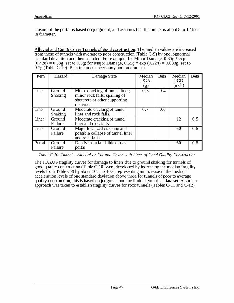
Appendices R47.01.02 Rev. 1. 7/12/2001


closure of the portal is based on judgment, and assumes that the tunnel is about 8 to 12 feetin diameter.

Alluvial and Cut & Cover Tunnels of good construction . The median values are increasedfrom those of tunnels with average to poor construction (Table C-9) by one lognormalstandard deviation and then rounded. For example: for Minor Damage, 0.35g * exp(0.428) = 0.53g, set to 0.5g; for Major Damage, 0.55g * exp (0.224) = 0.688g, set to0.7g (Table C-10). Beta includes uncertainty and randomness.



Beta

Liner GroundShaking


0.5 0.4

Liner GroundShaking


0.7 0.6

Liner GroundFailure


12 0.5

Liner GroundFailure


60 0.5



60 0.5

Table C-10. Tunnel – Alluvial or Cut and Cover with Liner of Good Quality Construction

The HAZUS fragility curves for damage to liners due to ground shaking for tunnels ofgood quality construction (Table C-10) were developed by increasing the median fragilitylevels from Table C-9 by about 30% to 40%, representing an increase in the medianacceleration levels of one standard deviation above those for tunnels of poor to averagequality construction; this is based on judgment and the limited empirical data set. A similarapproach was taken to establish fragility curves for rock tunnels (Tables C-11 and C-12).

Appendices R47.01.02 Rev. 1. 7/12/2001


Rock Tunnels of poor to average construction . The fragility curves are developed based onengineering judgment. (Table C-11), with adjustments taken from rock tunnels of goodquality construction. Beta includes uncertainty and randomness.



Beta

Liner GroundShaking


0.5 0.4

Liner GroundShaking


0.7 0.6

Liner GroundFailure


12 0.5

Liner GroundFailure


60 0.5



60 0.5

Table C-11. Tunnel – Rock without Liner or with Liner of Average to Poor QualityConstruction

Rock Tunnels of good construction . The median peak ground acceleration was derivedrecognizing that little damage occurs below 0.4g. It was assumed that the median PGA forminor damage to rock tunnels of good construction quality would occur one lognormalstandard deviation above 0.4g. (Table C-12). Beta includes uncertainty and randomness.



Beta

Liner GroundShaking


0.6 0.4

Liner GroundShaking


0.8 0.6

Liner GroundFailure


12 0.5

Liner GroundFailure


60 0.5



60 0.5

Table C-12. Tunnel – Rock without Liner or with Liner of Good Quality Construction

As of the time when the tunnel fragility curves were prepared for the HAZUS program(early 1990s), damage due to ground shaking that would results in closure of tunnels wasnot considered likely; therefore, there is no effect to the functionality of the tunnels due toground shaking in the damage algorithm. As will be described in subsequent sections, this

Appendices R47.01.02 Rev. 1. 7/12/2001


"heavy" damage state has in fact been occasionally observed, suggesting that the HAZUSfragility curves might need to be modified.

For ground failures (such as surface faulting through the interior of the tunnel), substantialpermanent ground deformations need to occur before appreciable damage occurs. Formoderate damage, a permanent ground deformation of one foot is used, and for majordamage, a permanent ground deformation of five feet is used. These displacements arebased on a typical water tunnel equivalent diameter of about 8 feet. For both moderate andmajor damage due to ground failure, tunnel closure is possible; tunnel closure could occurimmediately, or within a few days of the earthquake, either due to aftershocks, orcontinued erosion of the geology behind the failed liner.

If the tunnel portals are subjected to PGDs due to landslide, then the same PGDs (five feet)is assumed to cause tunnel major damage and closure. Rockfall type avalanches are notspecifically considered in the fragility curves.

C.1.2 Comparison of HAZUS and ATC-13 Fragility CurvesTable C-13 compares the median peak ground accelerations for fragility curves developedin Tables C-10 and C-12 (good quality construction) with the damage algorithms presentedin ATC-13 [ATC, 1985]. Only median values are compared because the dispersions in theATC-13 data do not reflect variability in the ground motion; whereas, the fragility curvesdeveloped here do. The damage probability matrices given in the ATC-13 were convertedto a cumulative probability distribution using the methodology described in ASCE [1985]and using MMI to PGA conversion suggested by McCann et.al. [1980] (Table C-14).

Tunnel Type / Damage State HAZUS (PGA) ATC-13 (PGA)RockModerate Damage 0.8 g 0.94 gMinor Damage ** 0.6 g 0.45 gCut & Cover or AlluvialModerate Damage 0.7 g 0.74 – 0.84 g *Minor Damage ** 0.5 g 0.40 – 0.44 g *

Table C-13. Comparison of Tunnel Fragility Curves

* ATC-13 gives values for Cut & Cover and Alluvial Tunnels. Both PGAs are given above.** For Minor Damage State shown above, the corresponding ATC-13 Damage State is Light.

MMI PGA Interval PGA UsedVI 0.09 – 0.15 0.12VII 0.16 – 0.25 0.21VIII 0.26 – 0.45 0.36IX 0.46 – 0.60 0.53X 0.61 – 0.80 0.71XI 0.81 – 0.90 0.86XII ≥ 0.91 1.15

Table C-14. Modified Mercalli to PGA Conversion [after McCann et al, 1980]

As can be seen in Table C-13, the median fragility values for the two damage states agreereasonably well.

Appendices R47.01.02 Rev. 1. 7/12/2001


C.2 Databases of Owen and Scholl, Sharma and JuddOwen and Scholl [1981] extended the database of Dowding and Rozen [1978] to a total of127 cases. Additions to the database included observations from the 1906 San Franciscoearthquake, 1971 San Fernando earthquake, and a number of less well documentedearthquakes around the world. Based on their examination of the data, Owen and Schollconcluded the following:

• Little damage occurred in rock tunnels for peak ground accelerations below 0.4g.

• Severe damage and collapse of tunnels from shaking occurred only under extremeconditions, usually associated with marginal construction such as brick or plainconcrete liners and lack of grout between wood lagging and the overbreak.

• Severe damage was inevitable when the underground structure was intersected by afault that slipped during an earthquake. Cases of tunnel closure appeared to beassociated with movement of an intersecting fault, landslide, or liquefied soil.

• Deep tunnels were safer (i.e., less prone to damage) than shallow tunnels.

• Damage to cut-and-cover structures appeared to be caused mainly by large increasesin lateral forces from the surrounding soil backfill.

• Earthquake duration appeared to be an important factor contributing to the severityof damage.

Sharma and Judd [1991] further extended the database to 192 reported cases. In this study,the relationships between observed damage and parameters of the earthquake, tunnelsupport system, and geologic conditions were examined. Parameters considered in theirstudy included earthquake magnitude, epicentral distance, peak ground acceleration, formof tunnel internal support and lining, overburden depth, and rock type. Sharma and Juddconcluded that:

• Damage incidence decreased with increasing overburden depth.

• Damage incidence was higher for colluvium than for harder rocks.

• Internal tunnel support and lining system appeared not to affect damage incidence.

• Damage increased with increasing earthquake magnitude and decreasing epicentraldistance (i.e., increasing peak ground acceleration).

• No or minor damage can be expected for peak accelerations at the ground surfaceless than about 0.15g.

C.3 Database of Power et alThe tunnel studies described in Sections C.1 and C.2, while informative and indicative ofgenerally good tunnel performance during earthquakes, contain some limitations:

• Many of the cases reported were observations from old and/or less welldocumented earthquakes; the locations and/or magnitudes of a number of theearthquakes were poorly defined.

Appendices R47.01.02 Rev. 1. 7/12/2001


• The ground shaking levels estimated for the cases were calculated using empiricalground motion attenuation relationships developed in early 1970’s. Peak groundaccelerations were estimated using distances from earthquake epicenters to thetunnel sites (i.e., epicentral distances). Ground motions calculated using epicentraldistance could be misleading for sites located close to a long or extended faultrupture area. Recently developed ground motion attenuation relationships generallyuse some measure of the closest distance from the site to the fault rupture area.Furthermore, recently developed attenuation relationships are better constrainedthan the older relationship by more data from many recent earthquakes.

• The damage cases reported and used in the previous studies included damageobservations resulting from direct fault rupture through a tunnel and other majorground failure mechanisms, such as landsliding and liquefaction. In examiningeffects of ground shaking on tunnels, cases of damage due to these other failuremechanisms should not be included.

To consider these limitations, Power et al. [1998] critically examined the previouslycompiled data bases summarized above and the following revisions were made:

• Data were removed for poorly documented earthquakes, such as earthquakes withunknown magnitudes or locations, or uncertain tunnel performance.

• Data were removed for cases of damage due directly to fault displacement,landsliding, or liquefaction, in order to examine trends for shaking-induced damagein the absence of ground failure.

• Data were not included for cut-and-cover tunnels or tubes, in order to developtrends and a correlation for bored tunnels only.

• Earthquake magnitudes were reported as moment magnitudes (Mw).

• Distances were evaluated as closest distances from the tunnel locations to the faultrupture surfaces of the earthquakes.

• Peak accelerations at the ground surface (at actual or hypothetical rock outcrops) atthe tunnel locations were estimated using recently developed ground (rock) motionattenuation relationships.

• Data were added from recent, moderate-to-large magnitude and better-documentedearthquakes: 1989 Loma Prieta, 1992 Petrolia, 1993 Hokkaido, 1994 Northridge,and 1995 Kobe earthquakes. Some data were added from case histories from olderearthquakes.

Table C-2 (entries 1 through 204) includes the complete database that is summarized inTable 6-1. Included in Table C-2 are information on the earthquake (name, date, andmoment magnitude), tunnel (name, owner, function, lining/support system, local geologicconditions, and thickness of geologic cover), level of ground shaking (peak groundacceleration), damage state, and references for data on the tunnels and tunnel performanceobservations.

In general, peak ground accelerations at the ground surface at tunnel locations wereestimated as median (50th percentile) values using rock ground motion attenuationrelationships developed by Sadigh et al. [1993, 1997] for earthquakes occurring on crustalfaults. The rock relationship of Youngs et al. [1993, 1997] for subduction zone

Appendices R47.01.02 Rev. 1. 7/12/2001


earthquakes were utilized for the 1964 Alaska earthquake. The median peak accelerationsfor the 1994 Northridge earthquake were estimated using event-specific ground motionattenuation relationship developed for the Northridge earthquake [Woodward-ClydeConsultants, 1995]. Rock ground motion attenuation relationships were utilized becausemost of the reported cases in the database involve tunnels founded in rock and also due tothe limited information that was available for the local geologic conditions. The actualground motions experienced at the depth of the tunnels would tend to be less than thevalues estimated for the ground surface in Table C-2 due to well-known tendencies forground motions to decrease with depth below the ground surface [e.g. Chang et al., 1986].The highest median peak rock acceleration estimated for the entire database is about 0.7g,for the 1923 Kanto, 1971 San Fernando, and the 1994 Northridge earthquakes. Manyestimated peak rock accelerations for the 1995 Kobe earthquakes are about 0.6g. The Kobeearthquake produced by far the most observations for moderate to high levels of shaking(numerous estimated median peak rock accelerations at the ground surface above thetunnels in the range of about 0.4g to 0.6g).

Damage to the tunnels was categorized into 4 states: none; slight, for minor cracking andspalling of the tunnel lining; moderate, for major cracking and spalling; and heavy for totalor partial collapse of a tunnel.

Figure C-2 presents a summary of the observations of the effects of seismic groundshaking on tunnel performance for the case histories 1 through 204 in Table C-2. Asindicated previously, the data are for damage due only to shaking and exclude damage thatwas definitely or probably attributed to fault rupture, landsliding, or liquefaction. Also, thedata are for bored tunnels only; data for cut-and-cover tunnels and tubes are not included.Figure C-2 shows the level of damage induced in tunnels with different types of liningssubjected to the indicated levels of ground shaking.

The following trends can be inferred from Figure C-2:

• For peak ground accelerations (PGAs) equal to or less than about 0.2g, groundshaking caused very little damage in tunnels.

• For peak ground accelerations (PGAs) in the range of about 0.2g to 0.5g, therewere some instances of damage ranging from slight to heavy damage.

• For peak ground accelerations (PGAs) exceeding about 0.5g, there were a numberof instances of slight to heavy damage.

• Tunnels having stronger lining system appeared to have performed better,especially those tunnels having reinforced concrete and/or steel linings.

It should be noted that the three instances of heavy damage (solid diamonds in Figure C-2)are all from the 1923 Kanto, Japan earthquake. For the 1923 Kanto earthquake observationwith PGA equal to 0.25g (see Table C-2 and Figure C-2), the investigations for this tunnelindicated that the damage may have been due to landsliding. In the other two observedoccurrences of heavy damage shown in Figure C-2, collapses occurred in the shallowportions of the tunnels.

The correlations observed in Figure C-2 show similar trends as those observed in theprevious study by Dowding and Rozen in Figure C-1. For relatively low ground shakinglevels, no or very little damage occurred for PGAs less than about 0.2g. There are relativefew instances of moderate to heavy damage for accelerations less than 0.5g, especially forstronger and well-constructed tunnels. This was evident during the 1995 Kobe, Japan

Appendices R47.01.02 Rev. 1. 7/12/2001


earthquake, where only a few cases of moderate damage and no major damage werereported for bored tunnels for peak ground accelerations of about 0.6g.

Although the number of observations for the seismic performance of cut and cover tunnelsare far fewer than those for bored tunnels, the available data including observations fromthe 1995 Kobe earthquake suggest that cut and cover box-like tunnels are more vulnerableto shaking than bored tunnels with more-or-less circular cross sections. Cut and covertunnels are vulnerable to racking-type deformations due to ground-imposed displacementsof the top of the box structure relative to the base. The higher vulnerability of cut-and-covertunnels as compared to bored tunnels is also probably due in part to the generally softergeologic materials surrounding the cut-and-cover structures, which are constructed atshallower depths than most bored tunnels.

C.4 Additions to Empirical DatabaseAsakura and Sato [1998] provided an expanded compilation of tunnel performance data forthe 1995 Kobe earthquake. Additional case histories obtained from their database duringthe present study are summarized in Table C-2 as entries 205 through 217.

As part of U.S./Japanese cooperative research and state-of-the-art studies of tunnel seismicdesign and performance by Prof. Thomas O’Rourke for MCEER, O’Rourke and Shiba[1997] summarized tunnel performance for 15 different earthquakes in Japan from 1923 to1993. Table C-3 summarizes tunnel damage observed in these earthquakes. Table C-4provides an explanation of the Japanese JMA intensity scale that is used in Table C-3.Figure C-3 shows a map of the locations of these earthquakes. The findings in Table C-3are similar to those described in the Sections C.2 and C.3 and included the followingobservations:

• Generally the parts of tunnels most significantly damaged were the portals, whichwas often attributed to landslides.

• Some of the most severe damage occurred due to fault movements.

• Generally, damage to tunnels due to shaking was associated with unreinforcedmasonry and unreinforced, cast-in-place concrete linings and with tunnel locationswhere construction difficulties were experienced and poor geologic conditions wereencountered.

• Significant damage to Japanese tunnels was observed predominately in locationswhere seismic intensities of V or higher on the JMA scale occurred (correlatingapproximately to MMI intensity VIII.

C.5 Tunnels with Moderate to Heavy Damage from GroundShakingAs previously discussed, the incidence of heavy damage (collapse of at least part of theliner system) in tunnels from ground shaking has been relatively rare. The followingsections summarize the specific tunnels which have collapsed, possibly due to groundshaking.

C.5.1 Kanto, Japan 1923 EarthquakeTable C-5 summarizes the earthquake damage observed in 34 tunnels after ten Japaneseearthquakes. These tunnels were selected as those displaying the most severe damage forwhich there is sufficient description in the literature (often in Japanese) to convey a

Appendices R47.01.02 Rev. 1. 7/12/2001


reasonably clear picture of the tunnel, earthquake, ground conditions, and nature of thedamage. The table summarizes information pertaining to tunnel location, use, length, cross-section, lining, geology, overburden, and damage observed either at, within, or beyond 30m from the portals.

Collapse (damage state 4 in Table C-5) beyond 30 m from the portals was observed in theabsence of landslides and faulting at a few tunnels, mostly in the 1923 Kanto earthquake.In all instances, the length of tunnel that experienced collapse was relatively small, rangingfrom 1.5 to 60 m. The following describes specific tunnel failures:

• The Mineokayama Tunnel (also see also EQID 10 in Table C-2) was underconstruction during the earthquake, and the collapse occurred in one of the drifts.The type and quantity of temporary support used in the drift were not reported.

• The Yose Railroad Tunnel (also see EQID 19 in Table C-2) was driven in soil for alength of 293 m at a distance from the epicenter of 48 km. The brick masonry liningwas 46-69 cm thick, with soil cover ranging mostly from 4 to 21 m. The JMAintensity was V-VI. During construction in 1900, water inflow attributed to a heavyrainfall resulted in the collapse of a 20-m-long section. During the Kantoearthquake, a 60-m-long section collapsed that included the section that failedduring construction. The collapsed section was about 55 m from the closest portal.

• The Toke Railroad Tunnel was driven in mudstone for a length of 353 m at adistance of 106 km from the epicenter, The brick masonry lining was 34-46 cmthick, with an overburden of 12 to 20 m. The JMA intensity was IV. There weresignificant inflows of water into the tunnel that persisted from the time of itsconstruction in 1894-95. During the Kanto earthquake, a section of the brick arch,2.7 m wide and 5.5 m long, failed, causing 90 m3 of rock and soil to collapse intothe tunnel.

C.5.2 Noto Peninsular Offshore, Japan 1993 EarthquakeTunnel collapses have been reported more recently for Japanese earthquakes. For example,Kunita, et al. (1994) report on the collapse of the Kinoura Tunnel as a result of the NotoPeninsular Offshore earthquake of 1993. The earthquake magnitude was 6.8, and thetunnel was located 26 km from the epicenter with a JMA intensity of approximately V. Thisroad tunnel was driven in 1965 through alternating strata of tuff and mudstone. The 76-m-long horseshoe-shaped tunnel was 6 m wide and about 4 m high. Timber supports wereused during construction, and the final lining was composed of 30-cm-thick concrete. Itappears that the lining was unreinforced. After the main shock, a 4.5 x 4.5 m section ofthe arch lining collapsed at a distance of 21 m form the nearest portal. An aftershock causedthe fall zone to expand, and two days after the main shock the tunnel was almostcompletely blocked with debris.

C.5.3 Kobe, Japan 1994 EarthquakeDuring the 1994 Kobe earthquake the cut-and-cover tunnel at the Daikai Subway Stationcollapsed catastrophically. It appears that this is the only instance of tunnel collapse as aresult of the Kobe earthquake. The performance of the Daikai Station has been covered inthe technical literature. Shear distortion from vertically propagating shear waves causedhinge formation where the central reinforced concrete columns were connected to the roofand invert. There was a lack of adequate confining steel in the central columns, whichhelped to promote column failure. See Figure C-4.

Appendices R47.01.02 Rev. 1. 7/12/2001


C.5.4 Duzce, Turkey 1999 EarthquakeTwin tunnels, each 18 m in excavated diameter, were significantly adversely affected by the1999 Duzce (Turkey) earthquake. They are located on Gurnosova-Gerede portion of theNorthern Anatolian Motorway. The tunnels were being driven in a faulted and deformedsequence of rocks, including flysch, shale, sandstone, marble, granite, and amphibolite.Tunneling was performed according to NATM principles, with shotcrete, rock bolts, andlight steel sets. The epicenter of the Mw 7.2 earthquake was located about 20 km from thewestern portals of the tunnels. The surface rupture of the causative fault was within 3 kmof these portals. Peak acceleration and velocity recorded at the nearest strong motion stationat Bolu (6 km from the causative fault) were 0.81 g and 66 cm/s, respectively.Observations show that the tunnels performed remarkably well, especially in light of theirclose proximity to the seismic source. Some of the temporary shotcrtete-supportedsections, however, collapsed where the worst ground conditions were located, and thesesections are discussed below.

• Adjacent twin sections collapsed in a fault zone with weak, intensely slickensidedclay gouge and crushed metacrystalline rock with the consistency of silty clay.About 300-m-long sections were affected by full or partial collapse, each locatedapproximated 240 m from the western portals. The tunnels in this location weresupported with a 75-mm-thick shotcrete lining with rock bolts and light steel sets.Substantial deformation had been observed in these sections of the tunnel duringconstruction, and it is likely that the initial lining had been subjected to considerablestress under static conditions.

• Partial collapse and severe initial lining deformation was observed near tunnelheadings being driven from the eastern portals at the opposite end of the 3.3-km-long highway tunnel. Five-meter-diameter tunnels were being driven as pilot benchtunnels along opposite sides of each 18-m-diameter highway tunnel. The intentionwas to drive the smaller tunnels initially through a fault zone, and then partially fillthem with concrete to act as reaction blocks for the shotcrete arch installed as theremaining parts of the heading were excavated. Each pilot bore tunnel wassupported with a 30-cm-thick shotcrete lining, patterned rock bolts, and light steelsets. The pilot bores were driven in a fault zone with weak, intensely slickensidedclay gouge. Thirty-meter-long sections of the pilot bores were affected bysignificant invert heave, ruptured and partially collapsed shotcrete, and buckledsteel sets.

C.5.5 Summary ObservationsFull or partial collapse of tunnels resulting from earthquakes has occurred under highlylocalized conditions, involving weak, wet, and highly fractured rock and soil. Collapse hasbeen confined to relatively short sections of tunnel. In Japan, tunnel collapse has occurredin linings with unreinforced masonry or unreinforced concrete. Failure of the DaikaiSubway Station (cut and cover tunnel) involved the failure of reinforced concrete columnswith inadequate confining steel. The collapsed tunnel sections in Turkey are located inweak, highly fractured clay gouge where construction was in progress and only the initialsupport system had been installed.

Both the Daikai Subway Station and Bolu Highway Tunnel were affected by near sourceground motions, involving high pulses of acceleration and velocity. Peak acceleration andvelocity measured at the Kobe Marine Meteorological Observatory (KMMO), which waswithin several km of the Dakai Station, were 0.81 g and 84 cm/s, respectively. The strongmotion recordings at Bolu, which were taken at distances comparable to those separatingthe Daikai Station and KMMO, show peak acceleration and velocity of 0.81 g and 66 cm/s.

Appendices R47.01.02 Rev. 1. 7/12/2001


Tunnel damage in these instances is associated with high velocity that would havepromoted high transient ground strains.

Accelerations inferred from JMA intensities are much less reliable than strong motionrecordings. The accelerations estimated in this way from Table C-5 for the Yose, Toke, andKinoura Tunnels are 0.25-0.40 g, 0.025-0.08 g, and 0.08-0.25 g, respectively.

In summary, there are two aspects of the strong motion that deserve attention. First, thenear source ground motion affecting the Daikai Station and Bolu Tunnel was high.Although both structures were influenced either by remarkably poor ground (Bolu Tunnels)or weakness in structural support (Daikai Station), they were nonetheless subjected tosignificant peak velocities. Collapsed tunnels, affected by the Kanto and Noto PeninsularOffshore earthquakes, were apparently subjected to a wide range of accelerations, some ofwhich were relatively small. The most prominent features of these tunnels affecting theirseismic vulnerability appears to be poor ground conditions in combination with anunreinforced masonry or concrete lining. It seems reasonable, therefore, to conclude thatpoor ground and weak lining conditions are the most important factors affecting seismicperformance leading to moderate to heavy damage. Strong motion in the near field cansupply significant excitation that will promote local collapse in tunnel sections influencedby poor ground and lack of either sufficient or final structural support.

Appendices R47.01.02 Rev. 1. 7/12/2001


C.6 Empirical Basis of the Tunnel Fragility CurvesTable C-2 presents the database of tunnels used in the development of fragility curvespresented in Section 6-3 of the main report. Table C-15 summarizes this dataset.

PGA (g) AllTunnels

DS = 1 DS = 2 DS = 3 DS = 4

0.07 30 30 0 0 00.14 19 18 1 0 00.25 22 19 2 0 10.37 15 14 0 0 10.45 44 36 6 2 00.57 66 44 12 9 10.67 19 3 7 8 10.73 2 0 0 2 0Total 217 164 28 21 4

Table C-15. Complete Bored Tunnel Database (Summary of Table C-2)

Tables C-16 through C-19 summarizes the dataset for based on bored tunnels with specificliner systems. Note that for a tunnel with multiple liner systems, the tunnel is classifiedaccording to the "best" liner type in the tunnel, according to the following ranking: unlined,timber / masonry / brick, unreinforced concrete, reinforced concrete / steel.

PGA (g) UnlinedTunnels

DS = 1 DS = 2 DS = 3 DS = 4

0.05 5 5 0 0 00.13 4 4 0 0 00.25 10 9 1 0 00.35 2 1 0 0 10.42 2 0 2 0 00.55 2 0 1 1 00.66 2 0 1 1 00.73 1 0 0 1 0Total 28 19 5 3 1

Table C-16. Unlined Bored Tunnels

Appendices R47.01.02 Rev. 1. 7/12/2001


PGA (g) Timber orMasonry

LinedTunnels

DS = 1 DS = 2 DS = 3 DS = 4

0.26 2 1 0 0 10.40 1 1 0 0 10.42 4 3 1 0 00.60 2 0 0 2 00.67 5 0 1 4 0Total 14 5 2 6 1

Table C-17. Bored Timber and Masonry / Brick Lined Tunnels

PGA (g) Unreinforced

ConcreteLined

Tunnels

DS = 1 DS = 2 DS = 3 DS = 4

0.08 13 13 0 0 00.13 6 5 1 0 00.23 3 2 1 0 00.38 8 8 0 0 00.45 33 28 3 2 00.57 53 39 9 4 10.67 8 1 4 3 00.73 1 0 0 1 0Total 125 96 18 10 1

Table C-18. Bored Unreinforced Concrete Lined Tunnels

PGA (g) ReinforcedConcrete /

SteelLined

Tunnels

DS = 1 DS = 2 DS = 3 DS = 4

0.07 9 9 0 0 00.15 5 5 0 0 00.27 6 6 0 0 00.35 4 4 0 0 00.45 4 4 0 0 00.57 6 3 2 1 00.66 4 2 1 0 1Total 38 33 3 1 1

Table C-19. Bored Reinforced Concrete or Steel Lined Tunnels

Appendices R47.01.02 Rev. 1. 7/12/2001


C.7 ReferencesAsakura, T., and Sato, Y., Mountain tunnels damage in the 1995 Hyogoken-Naubuearthquake, QR of RTRI, Vol. 39, No. 1, 1998.

Dowding, C.H. and Rozen, A., "Damage to Rock Tunnels from Earthquake Shaking",Journal of the Geotechnical Engineering Division, American Society of Civil Engineers,New York, NY, Feb. 1978.

ASCE, "Evaluation of Seismic Fragility and Validation of Probabilistic Models", TheFragility Evaluation/Validation Subgroup Joint Working Group on Seismic PRA of theASCE Dynamic Analysis Committee, Draft Report, April 1, 1985.

Chang, C.-Y., Power, M.S., Idriss, I.M., Somervile, P.G., Silva, W., and Chen, P.C.,Engineering characterization of ground motion – Task II: Observational data on spatialvariations of earthquake ground motion: Report prepared for U.S. Nuclear RegulatoryCommission, NUREG/CR-3805, Vol. 3, 1986.

Dowding, C.H. and Rozen, A., "Damage to Rock Tunnels from Earthquake Shaking",Journal of the Geotechnical Engineering Division, American Society of Civil Engineers,New York, NY, Feb. 1978.

HAZUS, Earthquake Loss Estimation Methodology, Technical Manual, Volume II,prepared by the National Institute of Building Sciences for Federal Emergency ManagementAgency, 1997.

Kunita, M., Takemata, R., and Lai, Y., "Restoration of a tunnel damaged by earthquake,"in Tunneling and Underground Space Technology, Vol. 9, No. 4, pp 439-448, 1994.

Kunita, M., et al., "Rehabilitation of Tunnel Damage caused by Noto Peninsula OffshoreEarthquake," Tunnels and Underground, Vol.24, No.11, pp.7-13, 1993 (in Japanese).

McCann, M.W., Sauter, F., and Shah, H.C., "A Technical Note on PGA-IntensityRelationship with Applications to Damage Estimation", BSSA, Vol. 7, No. 2, pp 631-637,1980.

O’Rourke, T.D. and Shiba, Y., Seismic performance and design of tunnels: AnnualReport, MCEER Highway Project, Sponsored by U.S. Department of Transportation,Federal Highway Administration, FHWA Contract DTFH61-92-C-00106, 1997.

Owen, G.N. and Scholl, R.E., "Earthquake Engineering a of Large UndergroundStructures", Federal Highway Administration and National Science Foundation,FHWA/RD-80/195, Jan. 1981.

Power, M.S., Rosidi, D., and Kaneshiro, J., Gilstrap, S.D., and Chiou, S.J., Summaryand evaluation of procedures for the seismic design of tunnels. Multidisciplinary Centerfor Earthquake Engineering Research, Technical Report MCEER-98-XXXX. DraftReport, September, 1998.

Sadigh, K., Chang, C.-Y., Abrahamson, N.A., Chiou, S.-J., and Power, M.S., 1993,Specification of long-period ground motions: updated attenuation relationships for rock siteconditions and adjustments factors for near-fault effects: Proceedings of AppliedTechnology Council Seminar on Seismic Isolation, Passive Energy Dissipation, and ActiveControl, Publication No. ATC-17-1 San Francisco, California, March 11-12, p. 59-70.

Appendices R47.01.02 Rev. 1. 7/12/2001


Sadigh, K., Chang, C.-Y., Egan, J.A. Makdisi, F.I., and Youngs, R.R., 1997,Atteunuation relationships for shallow crustal earthquakes based on California strongmotion data: Seismological Research Letters, Vol. 68, No. 1, p. 180-189.

Sharma, S., and Judd, W.R., 1991, Underground opening damage from earthquakes:Engineering Geology, Vol. 30.

Woodward-Clyde Consultants, 1995, Personal communication.

R47.01.02 Rev. 0

Tunnel Number

PGA - with No Damage

Tunnel Number

PGA - With Slight Damage

Tunnel Number

PGA - With Moderate Damage

1 0.075 1 0.185 1 0.2552 0.075 2 0.195 2 0.3403 0.08 3 0.225 3 0.4204 0.08 4 0.230 4 0.4805 0.08 5 0.250 5 0.4826 0.079 6 0.260 6 0.5107 0.99 7 0.300 7 0.5208 0.1 8 0.305 8 0.5259 0.12 9 0.420 9 0.550

1 0 0.12 1 0 0.460 1 0 0.5601 1 0.13 1 1 0.550 1 1 0.5901 2 0.13 1 2 0.550 1 2 0.6201 3 0.14 1 3 0.580 1 3 0.6401 4 0.14 1 4 0.580 1 4 0.6901 5 0.145 1 5 0.720 Mean 0.5130

1 6 0.15 Mean 0.3873 Std Dev 0.1163

1 7 0.16 Std Dev 0.1738

1 8 0.16

1 9 0.16Tunnel

NumberPGA - Portal Damage Only

2 0 0.16 1 0.515

2 1 0.1652 2 0.1652 3 0.172 4 0.182 5 0.1852 6 0.1852 7 0.19 Source Data2 8 0.19 Dowding, C.H. and Rozen, A.,2 9 0.19 "Damage to Rock Tunnels from Earthquake Shaking"3 0 0.19 Journal o fthe Geotechnical Engineering Division, ASCE, Feb. 19783 1 0.23 2 0.213 3 0.213 4 0.223 5 0.223 6 0.223 7 0.243 8 0.243 9 0.31

Mean 0.1834Std Dev 0.1429

Damage State

Mean Stnd Dev CoVariance Beta**2 BetaA=-0.5 * BETA**2

Median = Mean * exp(A)

None 0.1834 0.1429 0.779 0.474 0.689 -0.2370 0.145Minor 0.3873 0.1738 0.449 0.183 0.428 -0.0917 0.353Moderate 0.5130 0.1163 0.227 0.050 0.224 -0.0251 0.500

Table C-1. Raw Data - Tunnel Fragility Curves

R47.01.02 Rev. 0

EQID CASE EQNAME DATE Mw TNAME OWNER FUNLINER

SYSTEMROCK SOIL

COVER (M)

PGA (G) DS REFERENCE, NOTES

1 1-1 San Francisco, CA 1 8 / 4 / 0 6 7.8 SF #1 SPRR RR 4 R 2 4 0.41 1 Sharma & Judd, 1991




5 1-5 San Francisco, CA 1 8 / 4 / 0 6 7.8 Corte M. T, NPC RR 1 R 6 0 0.38 1 Sharma & Judd, 1991

6 1-6 San Francisco, CA 1 8 / 4 / 0 6 7.8 Pilarcitos Res #1 SFWD WT 4 R 6 8 0.65 1-3 Schussler, H., 1906

7 1-7 San Francisco, CA 1 8 / 4 / 0 6 7.8 Pilarcitos Res #2 SFWD WT 4 R 152 0.65 1-3 Schussler, H., 1906

8 1-8 San Francisco, CA 1 8 / 4 / 0 6 7.8 Pilarcitos Res #3 SFWD WT 4 R 137 0.69 1-3 Schussler, H., 1906

9 2-1 Kanto, Japan 1 / 1 0 / 2 7 7.9 Nagoye Nat. RW RR 1 3 0 0.40 2 Sharma & Judd, 1991

1 0 2-2 Kanto, Japan 1 / 1 0 / 2 7 7.9 Meno-Kamiana Nat. RW RR 4 R 1 7 0.60 3 Sharma & Judd, 1991

1 1 2-3 Kanto, Japan 1 / 1 0 / 2 7 7.9 Yonegami Yama Nat. RW RR 4 5 0 0.66 2 Sharma & Judd, 1991

1 2 2-4 Kanto, Japan 1 / 1 0 / 2 7 7.9 Shimomaki Matsu Nat. RW RR 4 2 9 0.69 3 Sharma & Judd, 1991

1 3 2-5 Kanto, Japan 1 / 1 0 / 2 7 7.9 Happon-Matzu Nat. RW RR 1 S 2 0 0.73 3 Sharma & Judd, 1991

1 4 2-6 Kanto, Japan 1 / 1 0 / 2 7 7.9 Nagasha-Yama Nat. RW RR 4-5 9 0 0.73 3 Sharma & Judd, 1991

1 5 2-7 Kanto, Japan 1 / 1 0 / 2 7 7.9 Hakone #1 Nat. RW RR 1 6 1 0.44 2 Sharma & Judd, 1991



1 8 2-10 Kanto, Japan 1 / 1 0 / 2 7 7.9 Hakone #7 Nat. RW RR 1 R 3 1 0.63 3 Sharma & Judd, 1991

1 9 2-11 Kanto, Japan 1 / 1 0 / 2 7 7.9 Yose Nat. RW RR 1 R 2 0 0.33 4 Sharma & Judd, 1991

2 0 2-12 Kanto, Japan 1 / 1 0 / 2 7 7.9 Doki Nat. RW RR 4 0.25 4 Sharma & Judd, 1991

2 1 2-13 Kanto, Japan 1 / 1 0 / 2 7 7.9 Namuya Nat. RW RR 5 7 5 0.52 4 Sharma & Judd, 1991

2 2 3-1 Kern County, CA 2 1 / 7 / 5 2 7.4 Saugus SPRR RR 1 R 4 0 0.06 1 Sharma & Judd, 1991

2 3 3-2 Kern County, CA 2 1 / 7 / 5 2 7.4 San Francisquito SPRR RR 1 R 160 0.08 1 Sharma & Judd, 1991

2 4 3-3 Kern County, CA 2 1 / 7 / 5 2 7.4 Elizabeth SPRR RR 1 R 250 0.10 1 Sharma & Judd, 1991

2 5 3-4 Kern County, CA 2 1 / 7 / 5 2 7.4 Antelope SPRR RR 1 R 3 0 0.16 1 Sharma & Judd, 1991

2 6 4-1 Alaska 2 7 / 3 / 6 4 8.4 Whittier #1 RR 1 R 400 0.22 2 Sharma & Judd, 1991

2 7 4-2 Alaska 2 7 / 3 / 6 4 8.4 Whittier #2 RR 1 R 350 0.21 1 Sharma & Judd, 1991

2 8 4-3 Alaska 2 7 / 3 / 6 4 8.4 Seward #1 RR 1 R 2 0 0.25 1 Sharma & Judd, 1991






3 4 5-1 San Fernando, CA 9 / 3 / 7 5 6.6 San Fernando MWD WT 5-6-7 S 4 5 0.69 2 Sharma & Judd, 1991

3 5 5-2 San Fernando, CA 9 / 3 / 7 5 6.6 Tehachapi #1 SPRR RR 1 R 3 0 0.04 1 Sharma & Judd, 1991



3 8 5-5 San Fernando, CA 9 / 3 / 7 5 6.6 Saugus SPRR RR 1 R 4 0 0.30 1 Sharma & Judd, 1991

3 9 5-6 San Fernando, CA 9 / 3 / 7 5 6.6 San Francisquito SPRR RR 1 R 160 0.24 1 Sharma & Judd, 1991

4 0 5-7 San Fernando, CA 9 / 3 / 7 5 6.6 Elizabeth SPRR RR 1 R 250 0.15 1 Sharma & Judd, 1991

4 1 5-8 San Fernando, CA 9 / 3 / 7 5 6.6 Antelope SPRR RR 1 R 3 0 0.10 1 Sharma & Judd, 1991

4 2 5-9 San Fernando, CA 9 / 3 / 7 5 6.6 Pacoima Dam WT 1 R 4 3 0.69 2 Sharma & Judd, 1991

4 3 6-1 Loma Prieta, CA 1 7 / 1 0 / 8 9 7.1 Fort Baker-Berry NPS HW 5 R 6 1 0.04 1 COE, NPS

4 4 6-2 Loma Prieta, CA 1 7 / 1 0 / 8 9 7.1 Presidio Park Caltrans HW 6 R 2 2 0.04 1 Yashinsky, 1998

4 5 6-3 Loma Prieta, CA 1 7 / 1 0 / 8 9 7.1 Alameda Creek Div SFWD WT 300 0.12 1 SFWD

4 6 6-4 Loma Prieta, CA 1 7 / 1 0 / 8 9 7.1 Coast Range SFWD WT 5 R 240 0.09 1 SFWD

4 7 6-5 Loma Prieta, CA 1 7 / 1 0 / 8 9 7.1 Pulgas SFWD WT 5 R 9 2 0.09 1 SFWD

4 8 6-6 Loma Prieta, CA 1 7 / 1 0 / 8 9 7.1 Irvington SFWD WT 5 R 122 0.10 1 SFWD

4 9 6-7 Loma Prieta, CA 1 7 / 1 0 / 8 9 7.1 Crystal Spr Baypass SFWD WT 5-6-7 R 7 6 0.09 1 SFWD

5 0 6-8 Loma Prieta, CA 1 7 / 1 0 / 8 9 7.1 Downtown S.F. Caltrain RR R 0.05 15 1 6-9 Loma Prieta, CA 1 7 / 1 0 / 8 9 7.1 Stanford Linear Collider SU AC 5 R 0.25 1 Rose, 1990; Fisher, 1989

5 2 6-10 Loma Prieta, CA 1 7 / 1 0 / 8 9 7.1 Lomita Mall 5 S 0.14 1 Kaneshiro, 1989

5 3 6-11 Loma Prieta, CA 1 7 / 1 0 / 8 9 7.1 Santa Teresa SCVWD WT 7 R 0.26 1 SCVWD

5 4 6-12 Loma Prieta, CA 1 7 / 1 0 / 8 9 7.1 Tunnel #5 SC,BT.PRR RR 3 R 0.40 1 SC,BT,PR

5 5 6-13 Loma Prieta, CA 1 7 / 1 0 / 8 9 7.1 Tunnel #6 SC,BT.PRR RR 3 R 0.28 1 SC,BT,PR

5 6 6-14 Loma Prieta, CA 1 7 / 1 0 / 8 9 7.1 Caldecott Caltrans HW 6 R 243 0.04 1 Yashinsky, 1998

5 7 6-15 Loma Prieta, CA 1 7 / 1 0 / 8 9 7.1 MacArthur Caltrans HW R 4 6 0.04 1 Yashinsky, 1998

5 8 6-16 Loma Prieta, CA 1 7 / 1 0 / 8 9 7.1 Stanford SFWD WT 5-7 R 2 3 0.14 1 SFWD

5 9 6-17 Loma Prieta, CA 1 7 / 1 0 / 8 9 7.1 Hillsborough SFWD WT 5-7 R 6 2 0.08 1 SFWD

Table C-2. Bored Tunnel Seismic Performance Database (Page 1 of 4)

R47.01.02 Rev. 0


SYSTEMROCK SOIL

COVER (M)


6 0 6-18 Loma Prieta, CA 1 7 / 1 0 / 8 9 7.1 Sunol Aqud. #1 SFWD WT 5 R 0.09 1 SFWD





6 5 7-1 Petrolia, CA 2 5 / 4 / 9 2 6.9 Tunnel #40 NCRR RR 5 S 0.13 1 NCRR

6 6 7-2 Petrolia, CA 2 5 / 4 / 9 2 6.9 Tunnel #39 NCRR RR 5-3 R 0.25 1 NCRR


6 8 7-4 Petrolia, CA 2 5 / 4 / 9 2 6.9 Tunnel #37 NCRR RR 5 R 0.15 1 NCRR








7 6 8-1 Hokkaido, Japan 0 / 0 / 9 3 7.8 Seikan HW 6 0.32 1 JTA, 1994

7 7 9-1 Northridge, CA 1 7 / 1 / 9 4 6.7 Pershing Sq St. LAMT RR 6 R 0.27 1 Tunnels & Tunneling, 1994

7 8 9-2 Northridge, CA 1 7 / 1 / 9 4 6.7 McArthur St. LAMT RR 6 R 0.27 1 Tunnels & Tunneling, 1994

7 9 9-3 Northridge, CA 1 7 / 1 / 9 4 6.7 Civic Center St. LAMT RR 6 R 0.27 1 Tunnels & Tunneling, 1994

8 0 9-4 Northridge, CA 1 7 / 1 / 9 4 6.7 Tun# 25 @ I-5/14 SPRR RR 5 R 9 2 0.67 2 METROLINK

8 1 9-5 Northridge, CA 1 7 / 1 / 9 4 6.7 Santa Susana SPRR RR 5 R 0.47 1 SPRR

8 2 9-6 Northridge, CA 1 7 / 1 / 9 4 6.7 Chatworth SPRR RR 5 R 0.50 1 SPRR

8 3 9-7 Northridge, CA 1 7 / 1 / 9 4 6.7 Chatworth SPRR RR 5 R 0.50 1 SPRR

8 4 9-8 Northridge, CA 1 7 / 1 / 9 4 6.7 Near I15 at Cajon Junc ATSF RR R 0.10 1 ATSF

8 5 9-9 Northridge, CA 1 7 / 1 / 9 4 6.7 Balboa inlet MWD WT 2-5-6-7 R 0.67 1 MWD

8 6 9-10 Northridge, CA 1 7 / 1 / 9 4 6.7 Balboa outlet MWD WT R 0.58 1 MWD

8 7 9-11 Northridge, CA 1 7 / 1 / 9 4 6.7 Castaic #1 MWD WT 6-7 R 0.29 1 MWD

8 8 9-12 Northridge, CA 1 7 / 1 / 9 4 6.7 Castaic #2 MWD WT 6-7 R 0.36 1 MWD

8 9 9-13 Northridge, CA 1 7 / 1 / 9 4 6.7 Saugus MWD WT 6-7 S 0.54 1 MWD

9 0 9-14 Northridge, CA 1 7 / 1 / 9 4 6.7 Placerita MWD WT 6-7 R 0.62 1 MWD

9 1 9-15 Northridge, CA 1 7 / 1 / 9 4 6.7 Newhall MWD WT 2-5-6-7 R 0.68 3-4MWD. Damage attributed to fluid pressure buildup behind tunnel and not to earthquake shaking

9 2 9-16 Northridge, CA 1 7 / 1 / 9 4 6.7 San Fernando MWD WT 5-6-7 R/S 0.50 1 MWD

9 3 9-17 Northridge, CA 1 7 / 1 / 9 4 6.7 Sepulveda MWD WT 5-7 R 0.27 1 MWD

9 4 9-18 Northridge, CA 1 7 / 1 / 9 4 6.7 Hollywood MWD WT R 0.22 1 MWD

9 5 9-19 Northridge, CA 1 7 / 1 / 9 4 6.7 San Rafael #1 MWD WT 6 R 0.16 1 MWD

9 6 9-20 Northridge, CA 1 7 / 1 / 9 4 6.7 San Rafael #2 MWD WT 6 R 0.18 1 MWD

9 7 9-21 Northridge, CA 1 7 / 1 / 9 4 6.7 Pasadena MWD WT 6 S 0.15 1 MWD

9 8 9-22 Northridge, CA 1 7 / 1 / 9 4 6.7 Siera Madre MWD WT S 0.13 1 MWD

9 9 9-23 Northridge, CA 1 7 / 1 / 9 4 6.7 Monrovia #1, #2 MWD WT 5-6 R 0.09 1 MWD

100 9-24 Northridge, CA 1 7 / 1 / 9 4 6.7 Monrovia #3 MWD WT 5-6 R 0.10 1 MWD

101 9-25 Northridge, CA 1 7 / 1 / 9 4 6.7 Monrovia #4 MWD WT 5-6 R 0.10 1 MWD

102 9-26 Northridge, CA 1 7 / 1 / 9 4 6.7 Glendora MWD WT 2-5-6-7 R/S 0.07 1 MWD

103 9-27 Northridge, CA 1 7 / 1 / 9 4 6.7 Oakhill MWD WT R 0.15 1 MWD

104 9-28 Northridge, CA 1 7 / 1 / 9 4 6.7 Ascat MWD WT R 0.14 1 MWD

105 9-29 Northridge, CA 1 7 / 1 / 9 4 6.7 Tonner #1 MWD WT 5-7 R 0.06 1 MWD

106 9-30 Northridge, CA 1 7 / 1 / 9 4 6.7 Tonner #2 MWD WT 5-7 R 0.06 1 MWD

107 9-31 Northridge, CA 1 7 / 1 / 9 4 6.7 LA Aqueduct LADWP WT 5 4 6 0.67 2 LADWP

108 10-1 Kobe, Japan 1 7 / 1 / 9 5 6.9 Rokkou (#1) JRN RR 5 460 0.60 3 Geo. Eng. Assn., 1996

109 10-2 Kobe, Japan 1 7 / 1 / 9 5 6.9 Kobe (#2) JRN RR 5 272 0.57 2 Geo. Eng. Assn., 1996

110 10-3 Kobe, Japan 1 7 / 1 / 9 5 6.9 Suma (#3) JRN RR 5 4 5 0.53 1 Geo. Eng. Assn., 1996

111 10-4 Kobe, Japan 1 7 / 1 / 9 5 6.9 Okuhata (#4) JRN RR 5 9 0 0.50 1 Geo. Eng. Assn., 1996

112 10-5 Kobe, Japan 1 7 / 1 / 9 5 6.9 Takatsukay(#5) JRN RR 5 8 5 0.49 1 Geo. Eng. Assn., 1996

113 10-6 Kobe, Japan 1 7 / 1 / 9 5 6.9 Nagasaka (#6) JRN RR 5 2 0 0.48 2 Geo. Eng. Assn., 1996

114 10-7 Kobe, Japan 1 7 / 1 / 9 5 6.9 Daiichinas (#7) JRN RR 5 150 0.55 1 Geo. Eng. Assn., 1996

115 10-8 Kobe, Japan 1 7 / 1 / 9 5 6.9 Ikuse (#8) JRN RR 5 250 0.57 1 Geo. Eng. Assn., 1996

116 10-9 Kobe, Japan 1 7 / 1 / 9 5 6.9 Daiichitaked(#9) JRN RR 5 9 5 0.43 1 Geo. Eng. Assn., 1996


R47.01.02 Rev. 0


SYSTEMROCK SOIL

COVER (M)


117 10-10 Kobe, Japan 1 7 / 1 / 9 5 6.9 Arima (#12) KBD RR 5 2 5 0.46 3 Geo. Eng. Assn., 1996

118 10-11 Kobe, Japan 1 7 / 1 / 9 5 6.9 Gosha (#13) KBD RR 5 4 0 0.41 1 Geo. Eng. Assn., 1996

119 10-12 Kobe, Japan 1 7 / 1 / 9 5 6.9 Kitakami (#14) HOE RR 6 350 0.51 3 Geo. Eng. Assn., 1996

120 10-13 Kobe, Japan 1 7 / 1 / 9 5 6.9 Iwataki (#15) HRP HW 5 135 0.58 3 Geo. Eng. Assn., 1996

121 10-14 Kobe, Japan 1 7 / 1 / 9 5 6.9 Nunohiki(#18) MRP HW 5 260 0.58 3 Geo. Eng. Assn., 1996

122 10-15 Kobe, Japan 1 7 / 1 / 9 5 6.9 Daini Nun (#19) MRP HW 5 240 0.58 2 Geo. Eng. Assn., 1996

123 10-16 Kobe, Japan 1 7 / 1 / 9 5 6.9 Hirano (#20) MRP HW 5 8 5 0.58 1 Geo. Eng. Assn., 1996

124 10-17 Kobe, Japan 1 7 / 1 / 9 5 6.9 K. Daiichi (#21) MRP HW 5 3 2 0.58 1 Geo. Eng. Assn., 1996

125 10-18 Kobe, Japan 1 7 / 1 / 9 5 6.9 K. Daini (#22) MRP HW 5 2 5 0.58 1 Geo. Eng. Assn., 1996

126 10-19 Kobe, Japan 1 7 / 1 / 9 5 6.9 Kamoetsu 1(#23) MRP HW 5 2 9 0.55 1 Geo. Eng. Assn., 1996



129 10-22 Kobe, Japan 1 7 / 1 / 9 5 6.9 Hiyodori (#26) MRP HW 5 4 0 0.54 1 Geo. Eng. Assn., 1996

130 10-23 Kobe, Japan 1 7 / 1 / 9 5 6.9 Shin-kobe 1(#27) MRP HW 5 330 0.49 2 Geo. Eng. Assn., 1996

131 10-24 Kobe, Japan 1 7 / 1 / 9 5 6.9 Shin-kobe 2(#28) MRP HW 5 330 0.49 2 Geo. Eng. Assn., 1996

132 10-25 Kobe, Japan 1 7 / 1 / 9 5 6.9 Karaki (#29) MRP HW 5 145 0.42 3 Geo. Eng. Assn., 1996

133 10-26 Kobe, Japan 1 7 / 1 / 9 5 6.9 Arino 1 (#30) MRP HW 5 2 5 0.39 1 Geo. Eng. Assn., 1996

134 10-27 Kobe, Japan 1 7 / 1 / 9 5 6.9 Arino 2 (#31) MRP HW 5 3 5 0.38 1 Geo. Eng. Assn., 1996

135 10-28 Kobe, Japan 1 7 / 1 / 9 5 6.9 Rokkousan (#32) MRP HW 5 280 0.51 2 Geo. Eng. Assn., 1996

136 10-29 Kobe, Japan 1 7 / 1 / 9 5 6.9 Shinohara (#33) MRP HW 5 1 5 0.55 1 Geo. Eng. Assn., 1996

137 10-30 Kobe, Japan 1 7 / 1 / 9 5 6.9 Hiyodori (#34) MRP HW 5 6 7 0.59 2 Geo. Eng. Assn., 1996

138 10-31 Kobe, Japan 1 7 / 1 / 9 5 6.9 Suma (#36) CDO 5 140 0.44 1 Geo. Eng. Assn., 1996

139 10-32 Kobe, Japan 1 7 / 1 / 9 5 6.9 Suma ext (#37) CDO 5 0.58 1 Geo. Eng. Assn., 1996

140 10-33 Kobe, Japan 1 7 / 1 / 9 5 6.9 Ibuki (#38) HHP HW 5 2 0 0.43 1 Geo. Eng. Assn., 1996

141 10-34 Kobe, Japan 1 7 / 1 / 9 5 6.9 Taizanji,1E(#39) HHP HW 5 5 3 0.44 1 Geo. Eng. Assn., 1996

142 10-35 Kobe, Japan 1 7 / 1 / 9 5 6.9 Taizanji,1W(#40) HHP HW 5 3 7 0.44 1 Geo. Eng. Assn., 1996

143 10-36 Kobe, Japan 1 7 / 1 / 9 5 6.9 Taizanji,2E(#41) HHP HW 5 2 5 0.45 1 Geo. Eng. Assn., 1996

144 10-37 Kobe, Japan 1 7 / 1 / 9 5 6.9 Taizanji,2W(#42) HHP HW 5 1 7 0.45 1 Geo. Eng. Assn., 1996

145 10-38 Kobe, Japan 1 7 / 1 / 9 5 6.9 Aina, E(#43) HHP HW 5 6 8 0.46 1 Geo. Eng. Assn., 1996

146 10-39 Kobe, Japan 1 7 / 1 / 9 5 6.9 Aina, W(#44) HHP HW 5 6 5 0.46 1 Geo. Eng. Assn., 1996

147 10-40 Kobe, Japan 1 7 / 1 / 9 5 6.9 Nagasaka.,E(#45) HHP HW 5 6 8 0.42 1 Geo. Eng. Assn., 1996

148 10-41 Kobe, Japan 1 7 / 1 / 9 5 6.9 Nagasaka.,W(#46) HHP HW 5 6 8 0.42 1 Geo. Eng. Assn., 1996

149 10-42 Kobe, Japan 1 7 / 1 / 9 5 6.9 T.Higa.,TOK(#47) JHP HW 5 6 2 0.58 1 Geo. Eng. Assn., 1996

150 10-43 Kobe, Japan 1 7 / 1 / 9 5 6.9 T.Higa.,KYU(#48) JHP HW 5 5 9 0.58 1 Geo. Eng. Assn., 1996

151 10-44 Kobe, Japan 1 7 / 1 / 9 5 6.9 T.Nishi,TOK(#49) JHP HW 5 4 2 0.57 1 Geo. Eng. Assn., 1996

152 10-45 Kobe, Japan 1 7 / 1 / 9 5 6.9 T.Nishi,KYU(#50) JHP HW 5 4 2 0.57 1 Geo. Eng. Assn., 1996

153 10-46 Kobe, Japan 1 7 / 1 / 9 5 6.9 Takak.,1TOK(#51) JHP HW 5 9 7 0.59 1 Geo. Eng. Assn., 1996

154 10-47 Kobe, Japan 1 7 / 1 / 9 5 6.9 Takak.,2TOK(#52) JHP HW 5 8 6 0.59 1 Geo. Eng. Assn., 1996

155 10-48 Kobe, Japan 1 7 / 1 / 9 5 6.9 Takak.,KYU(#53) JHP HW 5 8 7 0.59 1 Geo. Eng. Assn., 1996

156 10-49 Kobe, Japan 1 7 / 1 / 9 5 6.9 Tsuki.,TOK(#54) JHP HW 5 4 3 0.60 1 Geo. Eng. Assn., 1996

157 10-50 Kobe, Japan 1 7 / 1 / 9 5 6.9 Takak.,KYU(#55) JHP HW 5 3 4 0.60 1 Geo. Eng. Assn., 1996

158 10-51 Kobe, Japan 1 7 / 1 / 9 5 6.9 Omoteyama 1(#61) KTB RR 5 4 1 0.41 1 Geo. Eng. Assn., 1996

159 10-52 Kobe, Japan 1 7 / 1 / 9 5 6.9 Ochiai (#63) KTB RR 5 0.56 1 Geo. Eng. Assn., 1996

160 10-53 Kobe, Japan 1 7 / 1 / 9 5 6.9 Yokoo, 1 (#64) KTB RR 5 0.59 1 Geo. Eng. Assn., 1996

161 10-54 Kobe, Japan 1 7 / 1 / 9 5 6.9 Yokoo, 2 (#65) KTB RR 5 0.60 1 Geo. Eng. Assn., 1996

162 10-55 Kobe, Japan 1 7 / 1 / 9 5 6.9 Shiroyama (#66) JRN RR 5 0.58 1 Geo. Eng. Assn., 1996

163 10-56 Kobe, Japan 1 7 / 1 / 9 5 6.9 Nashio 2 (#67) JRN RR 5 0.48 1 Geo. Eng. Assn., 1996

164 10-57 Kobe, Japan 1 7 / 1 / 9 5 6.9 Takedo 2 (#68) JRN RR 5 0.40 1 Geo. Eng. Assn., 1996

165 10-58 Kobe, Japan 1 7 / 1 / 9 5 6.9 Douba 1 (#69) JRN RR 5 0.40 1 Geo. Eng. Assn., 1996



168 10-61 Kobe, Japan 1 7 / 1 / 9 5 6.9 Keietu (#76) KBD RR 5 0.58 1 Geo. Eng. Assn., 1996

169 10-62 Kobe, Japan 1 7 / 1 / 9 5 6.9 Nakayama(#77) KBD RR 5 0.58 1 Geo. Eng. Assn., 1996

170 10-63 Kobe, Japan 1 7 / 1 / 9 5 6.9 Kadoyama (#78) KBD RR 5 0.58 1 Geo. Eng. Assn., 1996

171 10-64 Kobe, Japan 1 7 / 1 / 9 5 6.9 Kudari (#79) KBD RR 5 0.54 1 Geo. Eng. Assn., 1996

172 10-65 Kobe, Japan 1 7 / 1 / 9 5 6.9 Kik, Nobori(#81) KBD RR 5 0.54 1 Geo. Eng. Assn., 1996

173 10-66 Kobe, Japan 1 7 / 1 / 9 5 6.9 Tanigami (#82) KBD RR 6 0.41 1 Geo. Eng. Assn., 1996

174 10-67 Kobe, Japan 1 7 / 1 / 9 5 6.9 Kobe (#84) KBD RR 0.56 1 Geo. Eng. Assn., 1996

175 10-68 Kobe, Japan 1 7 / 1 / 9 5 6.9 Aina (#85) KBD RR 0.48 1 Geo. Eng. Assn., 1996


R47.01.02 Rev. 0


SYSTEMROCK SOIL

COVER (M)


176 10-69 Kobe, Japan 1 7 / 1 / 9 5 6.9 Tetsukaiy (#87) MRP HW 5 2 0 0.60 1 Geo. Eng. Assn., 1996

177 10-70 Kobe, Japan 1 7 / 1 / 9 5 6.9 Taisanji (#88) MRP HW 5 5 0 0.44 1 Geo. Eng. Assn., 1996

178 10-71 Kobe, Japan 1 7 / 1 / 9 5 6.9 Kaibara (#89) MRP HW 5 2 0 0.36 1 Geo. Eng. Assn., 1996

179 10-72 Kobe, Japan 1 7 / 1 / 9 5 6.9 Shimohata (#91) MRP HW 5 2 0 0.60 1 Geo. Eng. Assn., 1996

180 10-73 Kobe, Japan 1 7 / 1 / 9 5 6.9 Fukuchi (#92) MRP HW 5 2 0 0.36 1 Geo. Eng. Assn., 1996

181 10-74 Kobe, Japan 1 7 / 1 / 9 5 6.9 Sumadera (#93) MRP HW 5 1 5 0.60 1 Geo. Eng. Assn., 1996

182 10-75 Kobe, Japan 1 7 / 1 / 9 5 6.9 Shin Arima (#95) MRP HW 5 2 0 0.48 1 Geo. Eng. Assn., 1996

183 10-76 Kobe, Japan 1 7 / 1 / 9 5 6.9 HigashiAina(#96) MRP HW 5 1 0 0.43 1 Geo. Eng. Assn., 1996

184 10-77 Kobe, Japan 1 7 / 1 / 9 5 6.9 Fukuyama (#97) MRP HW 5 1 5 0.59 1 Geo. Eng. Assn., 1996

185 10-78 Kobe, Japan 1 7 / 1 / 9 5 6.9 Minoya (#98) MRP HW 5 2 0 0.40 1 Geo. Eng. Assn., 1996

186 10-79 Kobe, Japan 1 7 / 1 / 9 5 6.9 Iwayama (#99) MRP HW 5 3 0 0.56 1 Geo. Eng. Assn., 1996

187 10-80 Kobe, Japan 1 7 / 1 / 9 5 6.9 Tamasaka (#100) MRP HW 5 1 0 0.58 1 Geo. Eng. Assn., 1996

188 10-81 Kobe, Japan 1 7 / 1 / 9 5 6.9 Fukiage (#101) MWB HW 5 3 0 0.44 1 Geo. Eng. Assn., 1996

189 10-82 Kobe, Japan 1 7 / 1 / 9 5 6.9 Maesaki (#102) MWB HW 5 1 0 0.43 1 Geo. Eng. Assn., 1996

190 10-83 Kobe, Japan 1 7 / 1 / 9 5 6.9 Nishikou 2 (103) MWB HW 5 2 0 0.39 1 Geo. Eng. Assn., 1996

191 10-84 Kobe, Japan 1 7 / 1 / 9 5 6.9 Fusehatagami (104) MWB HW 5 3 0 0.47 1 Geo. Eng. Assn., 1996

192 10-85 Kobe, Japan 1 7 / 1 / 9 5 6.9 Fusehatashita (105) MWB HW 5 3 0 0.47 1 Geo. Eng. Assn., 1996

193 10-86 Kobe, Japan 1 7 / 1 / 9 5 6.9 Enoshitayama (109) WT 4 3 7 0.60 3 Geo. Eng. Assn., 1996

194 10-87 Kobe, Japan 1 7 / 1 / 9 5 6.9 Motoyama (110) WT 9 6 0.59 3 Geo. Eng. Assn., 1996

195 10-88 Kobe, Japan 1 7 / 1 / 9 5 6.9 N. of Itayada St. KMS RR 6 0.60 1 Japan Society of Civil Eng, 1995

196 10-89 Kobe, Japan 1 7 / 1 / 9 5 6.9 Near Natani KMS RR 5 0.60 1 Japan Society of Civil Eng, 1995

197 10-90 Kobe, Japan 1 7 / 1 / 9 5 6.9 Koigawa river WT 6 0.60 1 Geo. Eng. Ass., 1996

198 10-91 Kobe, Japan 1 7 / 1 / 9 5 6.9 Hosoyadani WT 5 6 0.59 1 Geo. Eng. Ass., 1996

199 10-92 Kobe, Japan 1 7 / 1 / 9 5 6.9 Sennomori WT 5 3 0 0.59 2 Geo. Eng. Ass., 1996

200 10-93 Kobe, Japan 1 7 / 1 / 9 5 6.9 Shioyadani WT 5 2 5 0.59 2 Geo. Eng. Ass., 1996

201 10-94 Kobe, Japan 1 7 / 1 / 9 5 6.9 Kabutoyama-Ashiya HWC WT 5 2 5 0.58 1 Geo. Eng. Ass., 1996

202 10-95 Kobe, Japan 1 7 / 1 / 9 5 6.9 Sannomiya St. 3 UT 6 2 5 0.59 2 Geo. Eng. Ass., 1996

203 10-96 Kobe, Japan 1 7 / 1 / 9 5 6.9 NTT @ Chuo-ku NTT UT 6 S 0.60 2 Japan Society of Civil Eng, 1995

204 10-97 Kobe, Japan 1 7 / 1 / 9 5 6.9 Kansai Electric KEP UT 5 S 0.60 2 Japan Society of Civil Eng, 1995

205 Kobe, Japan 1 7 / 1 / 9 5 6.9 HIGASHIYAMA (#10) KER RR 4, 5 4-8 0.70 3 Asakura and Sato, 1998206 Kobe, Japan 1 7 / 1 / 9 5 6.9 EGEYAMA (#11) KER RR 4, 5 2-13 0.68 3 Asakura and Sato, 1998207 Kobe, Japan 1 7 / 1 / 9 5 6.9 MAIKO (UP) (#16) HSB HW 5 4-50 0.62 2 Asakura and Sato, 1998208 Kobe, Japan 1 7 / 1 / 9 5 6.9 MAIKO (DOWN) (#17) HSB HW 5 4-50 0.62 2 Asakura and Sato, 1998209 Kobe, Japan 1 7 / 1 / 9 5 6.9 SHIOYA-DAN (#35) KPW HW 5 4-80 0.70 3 Asakura and Sato, 1998210 Kobe, Japan 1 7 / 1 / 9 5 6.9 SEISHIN (2) (#58) KTB RR 6 7 0.36 1 Asakura and Sato, 1998211 Kobe, Japan 1 7 / 1 / 9 5 6.9 SEISHIN (1) (#59) KTB RR 6 3 0.37 1 Asakura and Sato, 1998212 Kobe, Japan 1 7 / 1 / 9 5 6.9 OMOTEYAMA (2) (#60) KTB RR 6 0.41 1 Asakura and Sato, 1998213 Kobe, Japan 1 7 / 1 / 9 5 6.9 KODERA (#62) KTB RR 6 7 0.47 1 Asakura and Sato, 1998214 Kobe, Japan 1 7 / 1 / 9 5 6.9 OBU (#86) KPW HW 5 5 0 0.55 1 Asakura and Sato, 1998215 Kobe, Japan 1 7 / 1 / 9 5 6.9 AINA (#90) KPW HW 5 2 0.43 1 Asakura and Sato, 1998216 Kobe, Japan 1 7 / 1 / 9 5 6.9 FUTATABI (#94) KPW 5 2 0 0.70 1 Asakura and Sato, 1998217 Kobe, Japan 1 7 / 1 / 9 5 6.9 SENGARI (#111) KWS WT 5 2-25 0.60 3 Asakura and Sato, 1998


R47.01.02 Rev. 0

EarthquakeDate and

Time Location of EpicenterMagnitude, JMA

IntensityArea Most Severely

Affected Tunnel Performance Selected References

1923 Kanto Sep. 1 Sagami Bay 7.90 Kanagawa and Extensive, severest damage JSCE [1984]11:58 AM 139.3 E, 35.2 N (unknown) VI Tokyo to more than 100 tunnels Yoshikawa [1979]

in southern Kanto area

1927 Kits-Tango Mar. 7 7 km WNW of Miyazu, Kyoto 7.30 Joint section of Very slight damage to 2 Yoshikawa [1979]6:27 PM 135.15 E, 35.53 N (0) VI Tango Peninsula railroad tunnels in the Yoshikawa [1984]

epicentral region

1930 Kita-Isu Nov. 26 7 km west of Atami, 7.30 Northerm part of Very severe damage to one Yoshikawa [1979]4:02 AM Shizuoka VI Izu Peninsula railroad tunnel due to Yoshikawa [1982]

139.0 E, 35.1 N (0) earthquake fault crossing

1948 Fukui June 28 12 km north of Fukui City 7.10 Fukui Plain Severe damage to 2 railroad Yoshikawa [1979]4:13 PM 136.20 E, 36.17 N (0) VI tunnels within 8 km from

the earthquake fault

1952 Tokachi-oki Mar. 4 Pacific Ocean 90 km ESE 8.20 Southern part of Slight damage to 10 rail- Committee Report [1954]10:23 AM of f the Cape Erimo VI - V Hokkaido road tunnels in Hokkaido Yoshikawa [1979]

144.13 E, 41.80 N (0)

1961 Kita-Mino Aug. 19 Border of Fukui and Gifu 7.00 Vicinity along the Cracking damage to a couple Okamoto, et al. [1963]2:33 PM Prefectures IV border of Fuikui of aqueduct tunnels Okamoto [1973]

136 46'E, 36 0l'N (0) and Gifu Prefs.

1964 Niigata June 16 Japan Sea 50 km NNE of 7.50 Nugata City Extensive damage to about JSCE [1966]1:01 PM Nugata City V - VI 20 railroad tunnels and Kawasumi [1968]

139 ll'E, 38 21'N (40) one road tunnel Yoshikawa [1979]

1968 Tokachi-oki May 16 Pacific Ocean 140 km 7.90 Aomori Prefecture Slight damage to 23 rail- Committee Report [1969]9:49 AM south off the Cape Erimo V road tunnels in Hokkaido

143 35~E, 40 44~N (0)

1978 Izu-Oshima-kinkai Jan. 14 In the sea between Oshima 7.00 South-eastern region of Very severe damage to 9 Onoda, et al. [1978]12:24 PM Isl. and Inatori, Shizuoka V VI Izu Peninsula railroad and 4 road tunnels Konda [1978]

139 15'E, 34 46N (0) in a limited area Yoshikawa [1979][(1982]

1978 Miyagiken-oki June 12 Pacific Ocean 115 km east 7.40 Sendai City and Slight damage to 6 railroad Committee Report [1980]5:14 PM of Sendai City, Miyagi V vicinity tunnels mainly existing in

142 l0'E, 38 09~N (40) Miyagi Prefecture

1982 Urakawa-oki Mar. 21 Pcific Ocean 18 km SW of 7.10 Urakawa-Cho and Slight damage to 6 railroad Yoshikawa [1984]11:32 AM Urakawa, Hokkaido IV - V Shizunsi-Cho, tunnels near Urakawa

142 36'E, 42 04'N (40) southern Hokkaido

1983 Nihonkai-chubu May 26 Japan Sea 90 km west of 7.70 Noshiro City and Slight damage to 8 railroad Yoshikawa [1984]11:59 AM Noshiro City, Akita V Oga City, Akita tunnels in Akita, etc. JSCE [1986]

139 04.6'E, 40 21.4'N (14)

1984 Naganoken-seibu Sep. 14 9 km SE of Mt. Ontake, 6.80 Otaki Village, Cracking damage to one Matauda, et al. [1985]8:48 AM Nagano VI - V Nagano headrace tunnel

137 33.6'E, 35 49.3'N (2)

1993 Notohanto-oki Feb. 7 Japan Sea 24 km north of 6.60 Suzu City Severe damage to one road Kitaura, et al. [1993]10:27 PM Suzu City, Ishikawa V tunnel Kunita, et al. [1993]

137 18'E, 37 39'N (25)

1993 Hokkaido-nansei-oki July 12 Japan Sea 86 km west of 8 Okushiri Isi. and Severe damage to one road Miyajima, et al. [1993]10:17 PM Suttsu, Hokkaido VI - V south-western part tunnel due to a direct hit Nishikawa, et al. [1993]

139 12'E, 42 47'N (34) of Hokkaido of falling rock JSEEP News [1993]

Table C-3. Tunnel Performance in Japanese Earthquakes

R47.01.02 Rev. 0

JMA Intensity Scale DefinitionAcceleration

(in gals)

0 No feeling Shocks too weak to be felt by humans and registered only by seismographs. < 0.8

I SlightExtremely feeble shocks felt only by persons at rest, or by those who are observant of earthquakes. 0.8 to 2.5

II WeakShocks felt by most persons; slight shaking of doors and Japanese latticed sliding doors (shoji). 2.5 to 8

III Rather StrongSlight shaking of houses and buildings, rattling of doors and shoji, swinging of hanging objects like electric lamps, and moving of liquids in vessels. 8 to 25

IV StrongStrong shaking of houses and buildings, overturning of unstable objects, and spilling of liquids out of vessels 25 to 80

V Very StrongCracks in sidewalks, overturning of gravestone and stone lanterns, etc.; damage to chimneys and mud and plaster warehouses 80 to 250

VI Disastrous Demolition of houses, but of less than 30% of the total, landslides, fissures in the ground. 250 to 400

VII Very Disastrous

Demolition of more than 30% of the total number of houses, intense landslides, large fissures in the ground and faults > 400

Table C-4. Japan Meteorological Agency Intensity Scale

R47.01.02 Rev. 0

ID Earthquake Name of Tunnel Location UseLength

(m)

Cross Section Width x Height

(m)

Liner System

Liner Thickness

(cm)Geological Feature

Cover (m)

Damage at Portals

Damge within 30 m of portals

Damage to Liner > 30 m from portal

Notes

1 1923 Kanto Hakone No. 1 (up) Yamakita-Yaga RR 284.7 4.3 x 4.7 4 34 - 57 marlstone, soil 2 2 1 (down) (on Tokaido [Gotemba) Line) 285.2 4.6 x 5.0 4 23 - 46

2 1923 Kanto Hakone No. 3 (up) Yamakita-Yaga RR 312.0 4.3 x 4.7 4 23 - 57 4 - 47 4 - slide 3 1 (down) (on Tokaido [Gotemba) Line) 318.1 4.6 x 5.0 4 23 - 46

3 1923 Kanto Hakone No. 4 (up) Yamakita-Yaga RR 269.9 4.3 x 4.7 4 23 - 57 4 - 53 4 - slide 3 1 Damage varies from Table C-2. (down) (on Tokaido [Gotemba] Line) 306.8 4.6 x 5.0 4 23 - 57

4 1923 Kanto Hakone No. 7 (up) Yaga - Surugaoyama RR 211.2 4.6 x 5.0 4 34 - 46 2 4 1 lesser damage to down (mountain side) (down) (on Tokaido [Gotemba] Line) 232.9 4.3 x 4.7 4 34 - 57 Damage varies from Table C-2.

5 1923 Kanto Nagoe (up) Kamakura - Zushi RR 442.6 4.9 x 6.0 4-5 34 - 46 mudstone 1 2 3 Damage varies from Table C-2. (down) (on Yokosuka Line) 344.3 4.3 x 5.6 4-5 23 - 57

6 1923 Kanto Komine Odawara - Hayakawa RR 260.5 9.1 x 6.0 (box) 4-5 126 - 137 soil 1 - 17 4 4 3 liner type depends on location(on Atami Tokaido] Line) 8.5 x 6.9 (tube) (Box section) (box section) (tube section)

7 1923 Kanto Fudoyama Hayakawa - Nebukawa RR 100.6 8.7 x 6.9 4-5 69 - 114 red agglomerate 4 - 20 2 2 1(on Atami Tokaido Line)

8 1923 Kanto Nenoueyama Hayakawa - Nebukawa RR 105.6 8.7 x 6.9 4-5 9 1 black agglomerate, 12 - 17 4 - slide 3 4 steep slope(on Atami Tokaido Line) pyroxene andesite

9 1923 Kanto Komekamiyama Hayakawa - Nebukawa RR 278.6 8.7 x 6.9 4-5 57 - 103 pyroxene andesite, 2 - 51 4 3 1 liner with invert arch(on Atami Tokaido Line) agglomerate, volcanic ash

1 0 1923 Kanto Shimomakiyayama Hayakawa - Nebukawa RR 160.9 8.7 x 6.9 4-5 69 - 103 pyroxene andesite, 14 - 31 4 - slide 4 1 steep slope(on Ataini [Tokaido] Line) volcanic ash Damage varies from Table C-2.

1 1 1923 Kanto Happonmatan Nebukawa - Manazurn RR 76.4 8.7 x 6.9 4-5 69 - 91 loose agglomerate < 17 4 - slide 3 1 steep slope(on Atami [Tokaido] Line)

1 2 1923 Kanto Nagasakayama Nebukawa - Manazurn RR 673.9 8.5 x 6.9 4-5 57 - 91 agglomerate 11 - 94 2 3 4 Damage varies from Table C-2.(on Atami Tokaido] Line)

1 3 1923 Kanto Yose Sagainiko - Fujino RR 292.6 4.6 x 5.0 4 46 - 69 soil 4 - 21 1 2 4 collapse accident reported during construction(on Chuo Line)

1 4 1923 Kanto Toke Toke - Ohami RR 353.3 4.3 x 4.5 4 34 - 46 mudstone 12 - 20 1 1 4(on Boso [Sotobo] Line)

1 5 1923 Kanto Namuya Iwal - Tomiura RR 740.3 4.9 x 6.0 4-5 30 - 57 shale, tuffite 9 - 70 2 3 4 steep slope, landslide suspected, (on Hojo [Uchibo] Line) water acceident reported during construction

1 6 1923 Kanto Mineokayama Futorni - Awakamogawa RR 772.5 4.9 x 6.0 4 30 - 47 sandstone, shale, gabbro 2 3 4 under construction at time of earthquake, (on Awa [Uchibo] Line) of drift progressive failure after the main shock

1 7 1930 Kita-Izu Tanna Atami - Kannami RR 7804.0 8.5 x 6.4 4-5 32 - 136 amdesite, agglomerate 1 1 4 under construction at time of earthquake, (on Atami [Tokaido] Line) earthquake fault crossing the tunnel

1 8 1961 Kita-Mino I Power Plant upperstream of Tedori WT 2538.0 2.1 x 2.2 5 20 - 40 sandstone, soil 1 1 3 cracking 32% of whole lengthRiver 2.4 x 2.45 5 20 - 40 longitudinal crck dominant

1 9 1964 Niigata Budo Murakami - Buya HW 320.0 8.6 x 5.8 5 50 - 60 rhyolite, talus, perlite clay 1 2 2 under construction at time of earthquake(on Route 7) cracking on the ground surface

2 0 1964 Niigata Terasaka Nezugaseki - Koiwagawa RR 79.4 4-5 47 - 107 soft mudstone 1 3 3 landslide area(on Uetsu Line) cracking on the ground

2 1 1964 Niigata Nezugaseki Nezugaseki - Koiwagawa RR 104.0 soft mudstone 2 2 2 landslide area(on Uetsu Line)

2 2 1968 Tokachi-oki Otofuke Nukabira - Horoka RR 165.0 4.8 x 5.2 4-5 25 - 60 tuf f < 50 1 1 3 landslide area, slope(on Shihoro Line)

2 3 1978 Izu-Oshima-kinkai Inatori Inatori - haihatna RR 906.0 4.4 x 5.1 5 40 - 70 metamorphic andesite < 90 3 2 3 earthquake fault crossing the tunnel(on Izu-kyuko Une) solfataric clay trouble with geology during construction

2 4 1978 Izu-Oshima-kinkai Okawa Okawa - Hokkawa RR 1219.5 andesite, fault clay 1 1 2 damage over 60 m long(on lzu-kyuko Une)

2 5 1978 Izu-Oshima-kinkai Atagawa Atagawa - Kataseshirata RR 1277.0 andesite, solfararic clay 1 1 2 damage over 400 m long(on Izu-kyuko Une)

2 6 1978 Izu-Oshima-kinkai Shiroyama Imaihama - Kawazu RR 4 1 1 a gigantic rock crashed and blocked(on Izu-kyuko Line) the portal

2 7 1978 Izu-Oshima-kinkai Tomoro Shirata - Inatori HW 425.5 5 andesite 3 3 3 cracking on the ground surface(on Higashi-Izu Toll Road)

2 8 1978 Izu-Oshima-kinkai Shirata Shirata - Inatori HW 88.7 audesite 4 - slide 2 3 steep slop(on Route 135) cracking on the ground surface

2 9 1978 Izu-Oshima-kinkai Joto Shirata - Inatori HW 127.3 4-6 audesite 4 - slide 1 4 steep slope(on Route 135) cracking on the ground surface

3 0 1978 Izu-Oshima-kinkai Kurone Shirata - Inatori HW 400.0 andesite, scoria 4 - slide 2 1(on Route 135)

3 1 1978 Miyagiken-oki Nakayama No.2 Naruko - Nakayamadaira RR 262.1 4.9 x 6.1 4-5 59 - 69 1 1 3(on Rikuu-east Line)

3 2 1984 Naganoken-seibu Otakigawa Dam Otaki, Nagano UT 2.7 x 3.0 5 sandstone, shale 1 1 2 earthquake fault crossing suspected

3 3 1993 Notohanto-oki Kinoura Orido, Suzu, Ishikawa HW 76.0 6.8 x 5.1 5 mudstone, tuff < 26 2 4 3 collapse extended by aftershocksShimamaki Village

3 4 1993 Hokkaido-nansei-oki Shiraito No. 2 (on Route 229) HW 1463.0 6 6 0 talus 1 1 4 falling rock hit the exposed tunnel lining

Table C-5. Tunnels with Moderate to Heavy Damage (Japanese)

Table C-6. Legend for Tables C-2, C-5

EQNAME : Earthquake nameMw: Moment MagnitudeTNAME : Tunnel nameOWNER OR REFERENCE:

ATSF = Santa Fe RailroadCALTRAIN = CALTRAIN (Bay Area commuter train)CALTRANS = California Department of TransportationCDO = City Development OfficeCOE = Corps of EngineersHHP = Hanshin Highway Public Corp.HOE = Hokoshin ExpressHRP = Hyogo Road Public Corp.HWC = Hanshin Waterworks CompanyHSB = Honsyu Shikoku Bridge AuthorityJHP = Japan Highway Public Corp.JRN = JR NishinipponJTA = Japan Tunneling AssociationKBD = Kobe DentetsuKEP = Kansai Electric PlantKER = Kobe Electric RailwayKMS = Kobe Municipal SubwayKPW = Kobe Public Works BureauKTB = Kobe Transportation BureauKWS = Kobe Water Supply BureauLADWP = Los Angeles Department of Water and PowerLAMT = Los Angeles MetroMRP = Municipal Road Public Corp.MWB = Municipal Waterworks BureauMWD = Metropolitan Water District of Southern CaliforniaNat. RW = National RailwayNCRR = North Coast RailroadNPC = North Pacific Coast RailroadNPS = National Park ServiceNTT = Nippon Telephone and TelegraphSC, BT, PR = Santa Cruz-Big Trees-Pacific RailwaySCVWD = Santa Clara Valley Water DistrictSFWD = San Francisco Water DepartmentSPRE = Southern Pacific RailroadSU = Stanford University

FUN: Function of tunnelAC = Particle acceleratorHW = HighwayRE = RailroadUT = UtilityWT = Water

Liner / support system1 = Unlined 2 = Rock Bolt 3 = Timber 4 = Masonry/brick5 = Unreinforced concrete 6 = Reinforced Concrete 7 = Steel pipe 9 = Unknown

Rock / SoilR = Rock S = Soil

COVER: Depth of cover above tunnel (meters)PGA : Peak Ground Acceleration in gDM : Damage State (Table C-3)

1 = None 2 = slight 3 = moderate 4 = heavyDM : Damage State (Table C-5)

1 = none2 = slight (cracks, displacement, deformation)3 = moderate (severe cracks, falling out, arch hanging down, swelling, invert cut)4 = heavy (collapse)

R47.01.02 Rev. 0

Case Number

Figure C-1. Peak Surface Acceleration andAssociated damage observations for earthquakes

(from Dowding and Rozen, 1978)

Figure C-2. Summary of empirical observations ofseismic ground shaking-induced damage for 204

bored tunnels [after Power et al, 1998]

Liner System

R47.01.02 Rev. 0

Figure C-3. Map of Japan showing locationsof 16 earthquakes in Tunnel Database

1995 Kobe(M=6.9)

R47.01.02 Rev. 0

Figure C-4. Deformations of cut and cover tunnel(exaggerated scale) for tunnel of

Kobe Rapid Transit Railwaybetween Daikai and Nagata stations

[after O'Rourke and Shiba, 1997]

R47.01.02 Rev. 0

Appendices R47.01.02 Rev. 1. 7/12/2001


D. Commentary - Canals

D.1 1979 Imperial Valley EarthquakeThe 1979 Imperial Valley M 6.5 earthquake caused widespread damage to irrigation canals.The following descriptions are adapted from [Dobry et al].

The Imperial Valley is located near the U.S. – Mexico border in Southern California. Thearea is flat, and thus landslide movements are not significant in this area. Water fordomestic, industrial and irrigation purposes originates at the Colorado River and istransported to a network of canals by the All American Canal. The canals are either linedwith unreinforced concrete or unlined.

The most extensively damaged canal was the All American Canal, constructed in the late1930s. The total damage to the canal was estimated to be about $982,000 [Youd andWieczorek]. Settlements, slumps, incipient slumps, and incipient lateral spreads occurredalong a 13 km long section between Drop No. 5 near the Ash Canal and the East HighlineCanal. The damage was concentrated on a 1.5 km long section of the All American Canal,near the Alamo River. The repairs were made rapidly, preventing detailed mapping of theembankment deformations. Rotational earth slumps threatened to breach the canal, incipientslumps, lateral spreads, and many undifferentiated fissures caused extensive cracks on theembankment and also in the compacted fill around the structures. Along the All AmericanCanal, the damage was distributed as far as 10 km east and 3 km west of the causativeImperial fault. Youd and Wieczorek reported that there was no evidence of large scaleliquefaction around the canal, but localized liquefaction may have contributed to failure insome places.

Slumping and incipient slumping extended for about 500 m along the east side of theHighline Canal.

Both sides of the South Alamo Canal were badly cracked for a length of about 100 m; crackwidths were about 15 mm and vertical crack offsets were 50 to 100 mm. At anotherlocation, the east bank showed fissures in a 500 m length. These fissures were caused byincipient slumping or lateral spreading towards the canal. The cracks at this site showed asmuch as 100 mm of opening and vertical offset.

The Barbara Worth Drain canal was also damaged in this earthquake.

In 1940, a M 7.1 earthquake occurred on much of the same fault as in the 1979 event. Inthe 1940 earthquake, damage to canals included: Holtville Main Drain, All American,Central Main, Alamo and Solfatara, for a total length of 119.7 km of damaged canal. Thedamage to these canals in the 1940 event was more severe than in the 1979 event. Althoughdamage to canals in the 1940 event was not clearly associated with the occurrence ofliquefaction, the soil in the affected areas did contain sand layers, whereas the soils in theareas without canal damage did not.

Based on damage to the canal and irrigation ditch network in the 1979 earthquake, theauthors analyzed the repair rate as a function of distance and recorded PGAs atrepresentative distances from the nearest fault rupture. The results are shown in Figure D-1. In Figure D-1a, "conduit" represents either canal or irrigation ditch. The followingtrends are noted:

• The repair rate is highest for locations closest to the fault. For PGAs in the range of0.5g to 0.8g, with corresponding PGVs of 22 in/sec to 35 in/sec, repair rates are

Appendices R47.01.02 Rev. 1. 7/12/2001


about 0.15 to 0.25 repairs per kilometer. Repair rates drop to about one-tenth thisrate when PGAs / PGVs have attenuated to about 0.2g / 9 in/sec.

• Due to the lack of detailed design information for each canal or ditch in the area, wedo not attempt to provide a fragility curve based on this information.

With regards to operation of the All American Canal in the 1979 earthquake, it was reported[EERI, 1980] that at the time of the earthquake, 3,700 cubic feet per second (cfs) of waterwas flowing in the canal. The bulk of this water was used for irrigation. Due to damage inthe canal, flow was reduced to about 700 cfs, in order to prevent flooding over damagedlevees of the canal. As repairs were made to the canal, flow was increased, reaching therequired flow of 4,100 cfs by October 19 (4 days after the earthquake). During this 4 dayoperation of the canal at low flows, there was sufficient raw water in an open cut reservoirfor the City of El Centro’s water treatment plant, and therefore the damage to the canal didnot directly affect treated water deliveries to customers in the City of El Centro (althoughdamage to distribution pipelines did affect treated water deliveries).

D.2 1980 Greenville EarthquakeContra Costa Canal. This canal is operated by the Contra Costa Water District. It transportsraw water from the Delta to the City of Concord, California, and other nearby localities.

This canal underwent minor levels of ground shaking in the 1980 Greenville earthquake.PGAs were on the order of 0.02g to 0.10g. Minor damage was observed due to earthsloughing from adjacent earthen banks.

D.3 1989 Loma Prieta EarthquakeContra Costa Canal. This canal underwent minor levels of ground shaking in the 1989Loma Prieta earthquake. PGAs were on the order of 0.02g to 0.10g. No damage wasobserved.

South Bay Aqueduct. This canal is operated by the State of California, Division of WaterResources. It transports water from the Delta to the Cities of Livermore, Pleasanton andSan Jose, California. This canal underwent moderate levels of ground shaking in the 1989Loma Prieta earthquake. However, no canal lining damage was sustained. A bridgeadjacent to the canal received moderate damage.

D.4 ReferencesDobry, R., Baziar, M. H., O'Rourke, T. D., Roth, B. L., and Youd, T. L., Liquefactionand Ground Failure in the Imperial Valley, Southern California During the 1979, 1981 and1987 Earthquakes, in Case studies of liquefaction and lifeline performance during pastearthquakes, Volume 2, United States Case Studies, Eds. T. D. O'Rourke and M.Hamada, NCEER Report 92-0002, February 17, 1992.

EERI, Imperial County, California Earthquake Reconnaissance Report , EarthquakeEngineering Research Institute, G, Brandow Coordinator, D. Leeds, Editor, February,1980.

Youd T.L. and Wieczorek G.F., Liquefaction and secondary ground failure in the ImperialValley California earthquake Oct 15, 1979, in The Imperial Valley California EarthquakeOct. 15, 1979, U.S. Geological survey, Professional Paper 1254, pp. 223-246, 1982.

Figure D-1. Canal and Ditch Repair Rates,1979 Imperial Valley Earthquake [after Dobry et al]

R47.01.02 Rev. 0

D-1a. Repair Rate versus Distance to Nearest Fault

D-1b. Repair Rate versus PGAs Recorded atSimilar Distances to the Nearest Fault

Appendices R47.01.02 Rev. 1. 7/12/2001


E. Basic Statistical ModelsAppendix E describes the general process used in establishing fragility curves.

E.1 The OptionsThere are three general approaches that can be used in developing fragility curves. Theseare:

• The empirical approach. This involves use of observed damage / non-damage frompast earthquakes.

• The analytical approach. This involves the use of specific engineeringcharacteristics of a component to assess its seismic capacity, in a probabilistic way.

• The engineering judgment approach. This involves the review of availableinformation by cognizant engineers, and making an informed judgment as to thecapacity of a component.

The main report uses all three approaches in developing fragility curves for the variouscomponents. Appendix E provides the mathematical models that are used in this process.Appendix G provides an alternate approach, called Bayesian Analysis, to standardregression analysis.

E.2 Randomness and Random VariablesRandomness in a parameter means that more than one value is possible. In other words theactual value, to some degree, is unpredictable. Mathematical representation of a randomvariable is thus a primary task in any probabilistic formulation.

In a loss estimation study, a prediction of the future is made using information from thepast, including experience and judgment whenever possible. Thus, it is necessary to collectall relevant information from the past for this purpose. A typical flow chart of the stepsinvolved is shown in Figure E-1. The information collected will constitute the samplespace.

Appendices A-D provide empirical information (sample space) for some of the watersystem components. The empirical information is likely not complete, and further effort inreviewing the performance of water transmission system components would likely yieldadditional information that could be added to the sample space. It was not feasible in thecurrent effort to consider every possible known piece of information. By expanding thedata in the sample space, it is hoped that better fragility curves can be developed in thefuture.

The randomness characteristics of any sample space can be described graphically in theform of a histogram, or a frequency diagram, as shown in Figure E-2. For a more generalrepresentation of the randomness, the frequency diagram can be fitted to some theoreticalprobability density function (PDF) fx(x). By integrating the probability density functionthus obtained, a cumulative distribution function (CDF) Fx(x) can be obtained.

To describe the PDF or CDF uniquely, some parameters of the distribution need to beestimated. The estimation of these parameters, which are called statistics, is a key step inthe development of fragility curves.

Appendices R47.01.02 Rev. 1. 7/12/2001


E.2.1 The Normal DistributionA random variable usually can be described mathematically by a distribution. A randomvariable can be discrete or continuous. Most commonly used discrete random variable aredescribed by the binomial distribution, Poisson, distribution, geometric distribution, etc.Continuous random variables are generally described by the normal distribution, lognormaldistribution, exponential distribution, Gamma distribution, Beta distribution, Chi-Squaredistribution, etc. The reader is referred to Benjamin and Cornell [1970] for a more completedescription of various distributions.

Amongst the most important statistical parameters are the mean value, µ, which denotes the

average of expected value of the random variable, and the standard deviation, σ, whichdenotes the dispersion of a random variable with respect to the mean value. The coefficientof variation (COV) is the ratio of the standard deviation and the mean value.

For a discrete random variable, the mean and unbiased variance can be calculated asfollows:

µx ii

n

nx=

=∑1

1

Var xn

xii

n

( ) =−

−( )=∑1

12

1

µ

The standard deviation and COV are calculated from the following relationships once themean and variance of a random variable are known.

σ x Var x= ( )

COV x

x= σ

µ

E.2.2 Which Distribution Model?To develop a probabilistic model, the underlying distribution of a random variable needs tobe known, as well as its statistics. The methods to empirically determine the distributionmodel is discussed in this section.

In practice, the choice of the probability distribution if often dictated by mathematicalconvenience. In many (most?) engineering evaluations of damage to water systemcomponents from past earthquakes, the functional form of the required probabilitydistribution may not be easy to determine, or more than one distribution may fit theavailable data. The basis of the properties of the physical process may suggest the form ofthe required distribution.

The required probability distribution may be determined empirically, based entirely on theavailable observed data., A frequency diagram for the set of data can be constructed and adistribution model can be selected by visual comparison as shown in Figure E-2.

When the distribution model is obtained using this method, or when two or moredistributions appear to be plausible probability distribution models, statistical tests (knownas goodness-of-fit tests for distributions) can be carried out to verify the distribution model.Two such tests commonly used for this purpose are the Chi-Square χ 2 and theKolmogorov-Smirnov (K-S) tests. For this report, the lognormal distribution is assumed inessentially all fragility formulations. This has been done as the lognormal distribution is

Appendices R47.01.02 Rev. 1. 7/12/2001


mathematically convenient; Section E.6 provides further details. Other researchers may findthat other dispersion models are better suited for specific applications.

E.2.3 Lognormal VariablesIn some special cases, suppose

Y X X Xn= • •1 2L

where Xi's are statistically independent lognormal variables with means µXi and standard

deviation σ Xi; then Y is also a lognormal variable.

From an engineering point of view, for loss estimation of water system components, theform of the lognormal distribution has some advantages. The total response, Y, can berepresented as the deterministic response value multiplied by a series of correction factorsthat are random and associated with various uncertainties. Irrespective of the properdistribution of these individual variables Xi, the product of the variable will beapproximately lognormal. Another advantage of the lognormal function is that a variablecannot take negative values. For these reasons, it is commonly adopted to model a variableas a lognormal variable rather than a normal variable. Note that whether or not the realworld is really "lognormal" is often ignored in the evaluation – but it is convenient that itshould be.

Knowing the mean and variance for a random variable X, µX and σ X the two parametersof the lognormal distribution λX (logarithmic mean) and ς X (logarithmic standard

deviation, beta, β) can be obtained as follows:

λ µ ςX X X= ( ) −ln12

2

and

ς σµX

X

X

22

21= +

ln

Say that xm is the median (x50) of the variable X. Then,

λ = ( )ln xm

and the 84th percentile value of X (i.e., one standard deviation higher than the median) is

x x e x em84 50= =β ς

Since Xi's are lognormal, then ln(Xi's) are normal and

λ λY Xi

n

Expected Value Yi

= ( ) ==∑_ ln

1

and

ς ςY Xi

n

Var Yi

2 2

1

= ( ) ==∑ln

Appendices R47.01.02 Rev. 1. 7/12/2001


E.2.4 Regression ModelsSome of the regression models used in this report for buried pipe are of the logarithmicregression form. In other words, if Yi is the repair rate per 1,000 feet and Xi is the PGV ininches/sec, then:

Y X zi iB

i= α

where α and B are constants to be determined from a regression analysis, and zi is the error

term. The solution for α and B using least squares methods can be found in many statisticstextbooks. Appendix G provides an alternative approach, called Bayesian analysis.

This model can be simplified into the standard linear regression model by taking the log ofthe equation, thus:

ln ln lnY B X ei i i= + +α

E.3 Simulation MethodsWhen performing loss estimates for water system components, the analyst can employ theMonte Carlo simulation technique. The Monte Carlo simulation technique is readily adaptedto computer techniques. One advantage of the technique is that many independent variablescan be processed on an individual basis, and the distribution of the dependent variable canbe examined by reviewing the results of many independent trials.

The number of simulations to be used will affect the accuracy of the final results. A largernumber of simulations will reduce the effects of the tails of the derived distribution.

E.4 Risk EvaluationUsing the procedures described in the previous sections, the uncertainties associated withthe random resistance R and the random load S can be quantified. This is graphicallyshown in Figure E-3. The shaded region in Figure E-3 indicates the region where theloading function (S) is greater than the resistance function (R). The risk that the damagestate R occurs is the area represented by the shaded region. Mathematically,

Risk P P R S

f r dr f s dsR

s

S

= ( ) = ≤( )

= ( )

( )∫∫

∞

damage state R occurs

00

E.5 Fragility Curve Fitting ProcedureFor the fragility curves developed for tanks and tunnels (Tables 5-7 and 6-3), a best fitregression analysis was performed. The approach was as follows:

The tanks and tunnels were "binned" into PGA bins. Each bin was for typically for a rangeof 0.1g, with the exception of PGAs over 0.7g. The higher g bins were wider, as therewere fewer tunnels in this PGA range. The PGA for each bin was set at the average of thePGA values for each tunnel in that bin. The percent of tunnels reaching or exceeding aparticular damage state was calculated for each bin.

A lognormal fragility curve was calculated for each of the damage states. A fragility curvewas calculated for all tanks or tunnels which reached damage state 2 (DS2) or above, DS3or above, DS4 or above, and DS5 (as applicable). The fragility curve uses two parameters:

Appendices R47.01.02 Rev. 1. 7/12/2001


the median acceleration to reach that damage state or above; and a lognormal dispersionparameter, β. The "best fit" fragility curve was selected by performing a least squareregression for all possible fragility curves in the range of A=0.01g to 5.00g (in 0.01gsteps) and β=0.01 to 0.80 (in 0.01 steps).

Since there are an unequal number of tanks or tunnels in each bin, the analysis wasperformed using just an unweighted regression analysis (eight data points for the eightbins), and also a weighted regression analysis (the number of data points in each binreflecting the actual number of tanks or tunnels in each bin). The weighted analysis isconsidered a better representation.

E.6 Randomness and UncertaintyIn developing or updating fragility curves, this report often separately characterizes"randomness" from "uncertainty".

Randomness reflects the variabilities in the real world, for which we do not have anadequate explanation using our current technology. In other words, no reasonable amountof additional study of the problem will reduce randomness. For example, there israndomness in the level of ground motion at two nearby sites, even if they have verysimilar soil profiles and distances from the fault rupture. We characterize Randomnessusing a logarithmic dispersion parameter:

βR

βR can be determined by doing regressions for ground motion attenuation functions for thesuitable parameter (PGA for tanks and tunnels, PGV and PGD for buried pipelines). Thereare many published references for these values, and it varies based on earthquakemagnitude, type of faulting mechanism, type of soil, etc. Recent work by Geomatrix(Power, Wells and Coppersmith, et al) can be used to provide βR for permanent grounddeformations (PGDs), for fault offset, liquefaction, and landslide.

Uncertainty reflects the uncertainty in our predictions, given the level of simplificationtaken in the analysis. For example, suppose a water utility wanted to do a "quick and dirty"earthquake loss estimate for buried transmission pipelines, without having to do a detailedeffort to ascertain exactly what type of buried pipelines are in use at which locations, howold they are, what is their leak history, which soils are most susceptible to corrosion,which soils are most susceptible to (PGDs), what level of corrosion protection has beentaken for a particular pipeline, etc. In such a case, the fragility curve used should take intoaccount that there is uncertainty in the pipeline inventory, as well as how that inventorywould respond to a given level of ground motion. We characterize Uncertainty using alogarithmic dispersion parameter:

βU

The total uncertainty is then expressed as:

β β βT R U= +2 2

E6.1 Total Randomness and UncertaintyThe method by which randomness and uncertainty is tabulated for this report considers thefollowing:

Appendices R47.01.02 Rev. 1. 7/12/2001


• A possible update of the water pipeline / transmission system component fragilitiesin the HAZUS computer program. HAZUS makes many simplifying assumptionsin order to get a computer program that is both easy to use and easy to program.Thus, only a single dispersion parameter is allowed in HAZUS, which is theequivalent of βT .

• Depending upon the source datasets used to establish the uncertainty parameters,the underlying uncertainty in the empirical data may or may not include βR . (Agood quality data set using GIS techniques on a well document earthquake wouldprimarily reflect βU ). In either case, the fragility curves in the main report must beclear as to whether the dispersion parameter includes (or does not include) βR . Byso doing, an the results in the main report can be suitably interpreted to allow forseparation of uncertainty in ground motion and inventory response.

• To summarize, it would be ideal to present three measures of uncertainty: βT (ifused in HAZUS or HAZUS-like programs); βR so that this could be varied by thetype of earthquake and by future advances in geotechnical descriptions of groundmotion; and βU so that this can be used in programs that are more sophisticatedthan HAZUS, and for end users who take the effort to establish a high qualityinventory database.

E.7 The Model to Estimate Fragility of a Structure or Piece ofEquipmentThe variability of how a structure or piece of equipment can respond can be described by aprobability density function (PDF), as shown in Figure E-3 (fR(r.)). In the greatpreponderance of application, the engineer rarely considers the shape of the PDF of theitem he/she is designing; instead, the engineer designs the item to "code". For convenience,we call designing to "code" a "deterministic" design. Generally conservative parameters areused in deterministic design so that only a low probability exists that the actual (random)seismic demand S exceeds the actual (random) seismic capacity. It is neither necessary nordesirable for the deterministic design to be so conservatively performed that the probabilityof failure is negligibly low (i.e., very close to zero).

In deterministic analysis, the deterministic factor of safety, FD, is defined as the ratio of thedeterministic code capacity, CD, to the deterministic computed response, RD, i.e.,

FC

RDD

D

=

In probabilistic analysis, both the capacity C and the response R are random variables.Thus, the factor of safety is given by:

FC

R=

which is also a random variable. A capacity factor, FC, can be defined as the ratio of theactual capacity, C, to the deterministic code capacity, CD. Similarly, a response factor, FR,is defined as the ratio of the deterministic computed response, RD, to the actual response R,i.e.,

Appendices R47.01.02 Rev. 1. 7/12/2001


FC

CF

R

RCD

RD= =;

Thus, the probabilistic factor of safety, F, can be defined in terms of the deterministicfactor of safety, FD, by:

F F F FC R D= • •

The probability of failure is the probability that the factor of safety, F, is less than 1. Thereliability is the probability that the factor of safety, F, is 1 or greater.

Computation of the probability of failure is tractable mathematically when the capacity andthe response factors, FD and FR, are assumed to be lognormally distributed randomvariables. F is a lognormal random variable if FD and FR, are lognormal random variables.The median value, F̂ , and the logarithmic standard deviation, βF of F are given by:

ˆ ˆ ˆF F F FC R D= • •

β β βF C R2 2 2= +

where ˆ ˆF FC R and are the median values and βC and βR and the logarithmic standarddeviations for the capacity FC, and response FR, factors. The probability of failure is thengiven by:

P Ff

F

=

Φln ˆ

1

β

where Φ is the standard cumulative distribution function.

Section E.7 is concerned with estimating the capacity factor random variable, FC, that,when combined with the response random variable, FR, and a code-specified deterministicfactor of safety, FD, can be used to estimate a probabilistic factor of safety F, and aprobability of failure.

Section 3 of the main report provides a brief introduction as to how to compute FR. It isbeyond the scope of the current effort to examine the issues with how to compute theseismic response at a location.

Under dynamic loading, the capacity factor is assumed to be made up of two parts:

F F FC S= • µ

where FS represents the strength factor for an equivalent static loading and Fµ represents theadded capacity due to the ductility (inelastic energy-absorbing capability) of the structureand the fact that the loading has limited energy content (short duration, cyclic loading).

E.8 ReferencesBenjamin, J. R. and Cornell, C. A., Probability, Statistics and Decision for CivilEngineers, McGraw-Hill.

Real World

RelevantInformation

SampleSpace

MathematicalRepresentation

Distribution StatisticalParameters

RiskEvaluation

Decisions

Figure E-1. Steps in a Probabilistic Study

R47.01.02 Rev. 0

Fre

quen

cy o

f Obs

erva

tions

Value of Random Variable X

Histogram PDF

Figure E-2. Typical Histogram or Frequency Diagram

R47.01.02 Rev. 0

Pro

babi

lity

Den

sity

R or S

Figure E-3. Risk Evaluation

R47.01.02 Rev. 0

fS(s) fR(r)

Failure Region

Appendices R47.01.02 Rev. 1. 7/12/2001


F. ExampleA portion of a California water transmission aqueduct built in 1930’s is examined inAppendix F. It consists of 33,400 feet of 62-inch diameter concrete pipe (with steelcylinder) and 48,000 feet of 66-inch diameter welded steel pipe.

For the purpose of illustrating how to apply the guideline procedures, this portion ofpipeline is further divided into the following four segments according to their surfacegeological conditions:

Segment Length Material JointAvg. Dist.from FaultConsidered

Surface Geology

1 7,200 ft Conc. w/steel cyl. Welded 2.3 mi. Rock-like soils

2 30,500 ft Steel Welded 0.6 mi. Firm soils

3 17,500 ft Steel Welded 1.5 mi. Firm Soils

4 26,200 ft Conc. w/steel cyl. Welded 3.7 mi. Rock-like soils

Table F-1. Water Transmission Aqueduct Example

Figure F-1 shows a simplified map of the water transmission system of Table F-1. Theissue at hand is to estimate the number of repairs may be required for this portion of thepipeline during an earthquake with Richter moment magnitude of 7.1 (MW7.1) generated bythe fault near the pipeline.

Tables F-2a and F-2b provides the summary results of the analysis.

Number of Repairs

LiquefactionSegment PGA GroundShaking Settlement

onlyWith Lateral

SpreadLandslide Total

1 [1] 0.58g 0.18 - - 0.18

2 [2] 0.55g 0.24 0.23 - - 0.47

3 [3] 0.40g 0.0 2.73 - 2.73

4 [4] 0.40g 0.60 - 1.49 2.09

Total - 1.02 0.23 2.73 1.49 5.47

Table F-2a. Summary Results (Dry Conditions)

Notes.[1]. Detailed calculation provided in Section F.1.[2]. Detailed calculation provided in Section F.2.[3]. Detailed calculation provided in Section F.3.[4]. Detailed calculation provided in Section F.4.

Appendices R47.01.02 Rev. 1. 7/12/2001


Number of Repairs

LiquefactionSegment PGA GroundShaking Settlement

onlyWith Lateral

SpreadLandslide Total

1 [1] 0.58g 0.18 - - 0.18

2 [2] 0.55g 0.24 0.23 - - 0.47

3 [3] 0.40g 0.0 2.73 - 2.73

4 [4] 0.40g 0.50 - 15.1 15.6

Total - 0.92 0.23 2.73 15.1 19.0

Table F-2b. Summary Results Wet Conditions)

Notes [1] to [4]. See Notes for Table F-2a.

F.1 Calculations – Segment 1Segment 1. This segment of welded steel pipeline is subject to strong ground shaking fromthe nearby fault. The pipe traverses an area best characterized as rock or rock-like materialwithout potential for liquefaction or landslide.

Ground Shaking

Step 1. Obtain anticipated earthquake magnitude generated from an active fault. Calculatethe site specific peak ground acceleration (PGA) from this earthquake.

Assume Mw = 7.1 and average PGA for this segment = 0.58g. The selection of the momentmagnitude is beyond the scope of this report. Section 3.2 of the main report provides someguidance, differentiating between deterministic and probabilistic definitions of earthquakes.Absent of input from knowledgeable seismologists, a rational approach would be toevaluated the pipeline for a specific scenario earthquake. Select the moment magnitude Mwfor the scenario earthquake based on the length of the fault (Lr in km), using an expressionlike:

log . .10 2 36 0 58L Mr w= − +

Once the magnitude of the scenario earthquake is selected, calculate the median horizontalground acceleration (PGA) such as by using equation F.1 (other equations might be moresuitable, depending upon location in the United States, type of fault mechanism, etc.). Thisassumes the pipeline is underlain by rock or rock-like soils.

ln . . . ln . .Z M R e M= − + − +( )[ ]− +1 274 1 1 2 1 0 48451 0 524 (eqn. F.1)

Assuming the average distance to the fault is 2.3 miles (= 3.7 km), gives ln Z = -0.543, orZ = 0.58g.

Step 2: Calculate peak ground velocity (PGV) with suitable attenuation relationship.

For M=7.1 and rock-like soil conditions, assume PGV = 49.4 cm/sec = 19.4 inch/sec.

Step 3: Calculate number of repairs per 1000 ft. based on PGV, pipe material, pipe joints,soil corrosiveness and pipe diameter.

Appendices R47.01.02 Rev. 1. 7/12/2001


From Table 4-4, the repair rate for the "backbone" pipe fragility curve is RR = 0.00187 *PGV = 0.0363 repairs per 1,000 feet. From Table 4-5, apply K1 = 0.7 (large diameterconcrete cylinder pipe with lap welded joints), so the total repair rate is 0.0254 repairs per1,000 feet.

Step 4: Calculate total number of repairs in this segment due to ground shaking

N = 0.0254 * 7200 / 1000 = 0.18.

F.2 Calculations – Segment 2Segment 2. This segment of welded steel pipeline is subject to strong ground shaking fromthe nearby fault. This segment also traverses reasonably competent soils which are subjectto localized liquefaction.

Ground Shaking

Step 1. Obtain anticipated earthquake magnitude generated from an active fault. Calculatethe site specific peak ground acceleration (PGA) from this earthquake.

Calculate the median horizontal ground acceleration (PGA) using an attenuation model suchas in Equation F.2 (others may be more suitable). This assumes the pipeline is underlain byfirm soils.

ln . . . ln . .Z M R e M= − + − +( )[ ]2 17 1 0 1 7 0 3825 0 5882 (eqn. F.2)

Assuming the average distance to the fault is 0.6 miles (= 1 km), gives Z = 0.55g.

Step 2: Calculate peak ground velocity (PGV) with suitable attenuation relationship.

For M=7.1 and firm soil conditions, PGV = 73.7 cm/sec = 29 inch/sec.

Step 3: Calculate number of repairs per 1000 ft. based on PGV, pipe material, pipe joints,soil corrosiveness and pipe diameter.

From Table 4-4, the repair rate for the "backbone" pipe fragility curve is RR = 0.00187 *PGV = 0.0543 repairs per 1,000 feet. From Table 4-5, apply K1 = 0.15 (large diametersingle lap welded steel pipe), so the total repair rate is 0.00814 repairs per 1,000 feet.

Step 4: Calculate total number of repairs in this segment due to ground shaking

N = 0.00814 * 30500 / 1000 = 0.25. But note that this value (N=0.25) assumes that theentire length of Segment 2 is not subject to liquefaction. As described below, about 4% ofthe length is subject to liquefaction. So, the damage in the ground shaking zone is 96% ofthis value (=0.96 * 0.25).

Liquefaction

Step 1: For a scenario earthquake, calculate the level of shaking (PGA) at the particularlocation of the component being evaluated.

M = 7.1, PGA = 0.55g (same as the value from the ground shaking calculations)

Note: Steps 2 through 5 below are to be used only when no detailedgeotechnical investigation is available. In any case, geotechnicalinvestigation done by knowledgeable professionals is stronglyrecommended.

Appendices R47.01.02 Rev. 1. 7/12/2001


Step 2: Establish the geologic unit for the near surface environment at the componentlocation.

From a site-specific geotechnical report or USGS or CDMG’s publications:

• Type of deposit: Alluvial.

• Age of deposit: Holocene

Chance of susceptibility to liquefaction is “Low”.

Step 3: Given the PGA, geologic unit and liquefaction susceptibility description, theestimated ground water depth and the magnitude of the earthquake, calculate the probabilitythat liquefaction occurs at the location.

For this PGA level, earthquake magnitude and ground water table, assume the probabilityof liquefaction is 80% for liquefiable deposits. Assume 5% of the deposits are liquefiable.Thus, the probability that a spcific location liquefies is 4% (=0.8 * 0.05).

Step 4: Given that the site liquefies, calculate the maximum permanent ground deformation(settlement) or the probabilities for different settlement ranges.

Assume the settlement ranges in Table F-3 are prepared using techniques outside the scopeof this report.

Settlement Range (in.) Probability of settlement due to 4% probability of liquefaction

≤ 1 4% * 35% = 1.4%

1 – 3 4% * 60% = 2.4%

3 – 6 4% * 4% = 0.16%

6 -12 4% * 1% = 0.04%

Table F-3. Settlement Ranges – Segment 2

Step 5: If there is no lateral spread (for example, the pipe is not adjacent to an open cut or aslope), calculate the repair rates per 1000 ft. using the vertical ground settlement.

From Table 4-4 and 4-6, the repair rate for the "backbone" pipe fragility curve is RR = K2* 1.06 * PGD repairs per 1,000 feet. From Table 4-6, apply K2 = 0.15 (large diametersingle lap welded steel pipe). The vertical displacement will be the total estimated PGDparameter.

The average values of the settlement ranges in the first column of Table F-3 are used as theestimated PGDs.

Assumedestimated PGD

(in.)

Number of repairs per 1000 ft. (Assume100% probability for each estimated

PGD)

Number of repairs per 1000ft.

1 n = 0.15 * 1.06 * (1)0.319 = 0.16 n = 0.16 * 1.4% = 0.00224

2 n = 0.15 * 1.06 * (2)0.319 = 0.20 n = 0.20 * 2.4% = 0.0048

4 n = 0.15 * 1.06 * (4)0.319 = 0.25 n = 0.25 * 0.16% = 0.00040

9 n = 0.15 * 1.06 * (9)0.319 = 0.32 n = 0.32 * 0.04% = 0.00013

Table F-4. Pipe Repair Rates – Segment 2

Appendices R47.01.02 Rev. 1. 7/12/2001


Repair rate per 1000 feet = 0.00224 + 0.0048 + 0.00040 + 0.00013 = 0.0076.

Step 6: Calculate total number of repairs in this segment due to liquefaction.

N = .0076 * 30,500 / 1000 = 0.23.

Note. The PGD algorithm already includes damage due to PGV.

Step 7: Total Repairs (Ground Shaking and Liquefaction) for Segment 2

The total number of repairs for Segment 2:

Liquefaction zone: N = 0.23

Ground shaking zone without liquefaction:

N = 0.25 * 0.96 = 0.24

Total = 0.23 + 0.24 = 0.47.

F.3 Calculations – Segment 3Repair rates for liquefaction (with and without lateral spread) are calculated. Assume M =7.1 and average PGA for this segment = 0.5g. The pipeline is assumed to be buried andtraverse through liquefiable soils near a body of water. It is also assumed that the pipe hasbeen installed using typical cut and cover trench techniques without special soilimprovement to address liquefaction hazards. While the soil within the pipeline trench maybe of various materials, the native soils underlying and adjacent to the pipe trench areassumed to control the overall potential for PGDs along the length of pipeline.

Liquefaction


M = 7.1, PGA = 0.40g. Note that for this segment, the pipe traverses modern young soils,and moderately high values of PGA (0.4g) may still have very high values of PGV (over35 inches / sec).

Note: Steps 2 through 6 below are to be used only when no detailedgeotechnical investigation is available. In any case, geotechnicalinvestigation done by knowledgeable professionals is stronglyrecommended.

Step 2: Establish the geologic unit for the near surface environment at the componentlocation.

From a site-specific geotechnical report or USGS or CDMG’s publications:

• Type of deposit: Delta.

• Age of deposit: Modern

Chance of susceptibility to liquefaction is “Very High”.

Step 3: Given the PGA, geologic unit and liquefaction susceptibility description, theestimated ground water depth and the magnitude of the earthquake, calculate the probabilitythat liquefaction occurs at the location.

Appendices R47.01.02 Rev. 1. 7/12/2001


For this PGA level, earthquake magnitude and ground water table, assume the probabilityof liquefaction is 95% for liquefiable deposits. Assume 25% of the deposits are liquefiable.Thus, the probability that a specific location liquefies is 24% (=0.95 * 0.25).

Step 4: Given that the site liquefies, calculate the maximum permanent ground deformation(settlement and lateral spread) and the probabilities for different PGD ranges.

Step 4a. No Lateral Spread. Table F-5 provides a range of settlements for the specific soildeposits and earthquake conditions.

Settlement Range (in.) Probability of settlement due to 24% probability of liquefaction

1 - 3 24% * 5% = 1.2%

3 - 6 24% * 25% = 6%

6 - 12 24% * 50% = 12%

> 12 24% * 20% = 4.8%

Table F-5. Settlement Ranges – Segment 3

Step 4b. With Lateral Spread. Assume an analysis is performed that determines that alateral spread with PGD = 82 inches is possible at locations so susceptible.

Step 5: For areas with no lateral spread, calculate the repair rates per 1000 ft. using thevertical ground settlement.

From Table 4-4 and 4-6, the repair rate for the "backbone" pipe fragility curve is RR = K2* 1.06 * PGD repairs per 1,000 feet. From Table 4-6, apply K2 = 0.15 (large diametersingle lap welded steel pipe). The vertical displacement will be the total estimated PGDparameter.

The average values of the settlement ranges in the first column of Table F-6 are used as theestimated PGDs.

Assumedestimated PGD

(in.)

Number of repairs per 1000 ft. (Assume100% probability for each estimatedPGD)

Number of repairs per 1000ft.

2 n = 0.15 * 1.06 * (2)0.319 = 0.20 n = 0.20 * 1.2 % = 0.0024

4 n = 0.15 * 1.06 * (4)0.319 = 0.25 n = 0.25 * 6.0 % = 0.015

9 n = 0.15 * 1.06 * (9)0.319 = 0.32 n = 0.32 * 12 % = 0.038

12 n = 0.15 * 1.06 * (12)0.319 = 0.35 n = 0.35 * 4.8 % = 0.017

Table F-6. Pipe Repair Rates – Segment 3

Repair rate per 1000 feet = 0.0024 + 0.015 + 0.038 + 0.017 = 0.072 (settlement only)

Step 6: For area adjacent to an open cut (lateral spread possible), calculate the repair ratesper 1000 ft. using the vector sum of the ground settlement and the lateral displacement.

The vector sum of the ground settlement and the lateral spread displacement should be usedfor PGD when lateral spread is possible. Assume the most probable settlement range is 6 to12 inches. Conservatively, use the high value to calculate PGD.

∴ 83)82()12( 22 =+=PGD in.

K2 = 0.15 (steel pipe with welded joints) per Table 4-6.

Appendices R47.01.02 Rev. 1. 7/12/2001


Repair rate per 1000 feet = 0.15 * 1.06 * (83)0.319 = 0.65 (lateral spread and settlement)

As the repair rate with lateral spread (0.65) is higher than the repair rate from settlementonly (0.072), use the higher value in zones with liquefaction with potential for lateralspread.

Step 7: Total Repairs (Ground Shaking and Liquefaction) for Segment 3


Liquefaction zone: N = 0.24 * 0.65 * 17,500 / 1,000 = 2.73

Check damage rate if there were no liquefaction.

Assume PGV = 35 inches per second. RR = 0.15 * 0.00187 * 35 = 0.0098 per 1,000 ft

N = 0.76 * .0098 * 17,500 / 1,000 = 0.13. since 0.13 << 2.73, liquefaction rate controls.

F.4 Calculations – Segment 4Repair rates for Segment 4 include the potential for landslide hazard along this length ofpipeline. It is assumed that the entire Segment 4 length is located in sloped terrain.

Landslide


Assume average PGA for this segment = 0.4g, and the typical soil profile is rock. Whilelandslide zones may be characterized as having up to a few tens of feet of colluvial material,it is still reasonable to use a rock-type attenuation model to estimate ground motions at thepipe locations.

∴Ais = 0.4g

Note: Steps 2 thru 4 below are to be used only when no detailedgeotechnical investigation is available. In any case, geotechnicalinvestigation done by knowledgeable professionals is stronglyrecommended.

Step 2: Determine slope angle and geologic group of the region or subregion beingevaluated.

Slope: 20° to 30° (based on site survey). Geologic Group: Weakly cemented rock.

Step 3: Determine the susceptibility category, the critical acceleration, ac, and the percentageof the landslide susceptibility area that is expected to be susceptible to landslide during dryand wet conditions.

Dry condition : ⇒ ac = 0.30g

Wet condition : ⇒ ac = 0.10g

Assume the following percentage of the pipeline lengths that are within susceptible soils:

Dry condition: ⇒ Percentage of Map Area with Landslide Susceptible Deposit = 8%

Wet condition: ⇒ Percentage of Map Area with Landslide Susceptible Deposit = 25%

Appendices R47.01.02 Rev. 1. 7/12/2001


Step 4: Estimate amount of PGD due to landslide based the critical acceleration (ac), theinduced acceleration (ais), and the expected number of cycles.

Dry condition:

E[PGD] = 0.57 in.

Wet condition:

E[PGD] = 23 in.

Step 5: Calculate the repair rates for dry and wet conditions.

Dry condition:

N = 0.8 * 1.06 * (0.57)0.319 = 0.71 per 1000 ft (covers 8% of pipe length)

N = 0.08 * 0.71 * 26,200 / 1,000 = 1.49 repairs.

Wet condition:

N = 0.8 * 1.06 * (23)0.319 = 2.31 per 1000 ft (covers 25% of pipe length)

N = 0.25 * 2.31 * 26,200 / 1,000 = 15.1 repairs.

Step 6: Total Repairs (Ground Shaking) for Segment 4


Assume PGV = 0.4g * 85 cm/g = 13.4 inches per second.

RR = 1.0 * 0.00187 * 13.4 = 0.025 per 1,000 ft

N = 0.92 * 0.025 * 26,200 / 1,000 = 0.60 (dry conditions)

N = 0.75 * 0.025 * 26,200 / 1,000 = 0.50 (wet conditions)

Lake

Hills

Fault

Segment 1

Segment 2

Segment 3

Segment 4

Figure F-1. Example WaterTransmission System

��

Appendices R47.01.02 Rev. 1. 7/12/2001


G. Bayesian Estimation of Pipe Damage

G.1 IntroductionAppendix G provides an alternative approach for developing fragility curves for estimatingdamage potential for buried pipelines.

As described in Section 4.6.2 of the main report, the complete empirical dataset exhibits alot of scatter. It is the judgment of the authors of the report that the form of the fragilityfunction used to describe damage to buried pipelines due to wave passage effects is to use astraight line through the entire dataset. Alternative approaches were investigated in the mainreport, including a power model. The decision to use a straight line through the dataset,fitted so that 50% of the empirical data points lied below and 50% lied above the curve,was selected for the following reasons:

• The scatter in the empirical dataset is large. Many different types of curves can be fittedthrough the dataset, but no one would be much better than the other, other thanmathematical convenience.

• The theoretical basis for estimating strain in the ground from wave propagation is that itis linearly correlated with maximum ground velocity. For wave propagation, pipe strainis often assumed to be the same as the ground strain, which basically assumes that thepipe does not slide relative to the ground.

• The desired accuracy of the fragility model for ground shaking is perhaps not asimportant as that for permanent ground deformations. This is because the rate ofpipeline damage in soils prone to PGDs is often an order of magnitude larger than therate of pipeline damage in soils not prone to PGDs.

• Regression analyses which use weighted damage data (Figure A-15) shows that thebest fit curve through the empirical data has an exponent of 0.99 (RR = 0.001795 *PGV0.99), which is essentially linear.

• Bayesian analyses presented in Section G.10 for cast iron pipe with diameters 6" and8" (the most common type) show a linear trend (exponent of 0.9942).

Any method used to fit a fragility function through the pipeline empirical database must dealwith the form of the empirical database. Specifically, the empirical database has thefollowing issues which might influence how one fits a fragility function through it:

• The empirical data is expressed in terms of repairs per length of pipeline (repairs per1,000 feet or repairs per km). Each empirical data point is ideally developed bycalculating the actual PGV for each pipe of homogeneous attribute. A homogeneousattribute for a pipe mean that the pipe has the same material, same joinery, samediameter, same lay lengths, same installation method, same age, same corrosionprotection system, same level of ground shaking, etc. The repair rate is calculated byadding up the entire length of pipe that experienced the same (or nearly the same) levelof ground motion, and by adding up all the repairs made to that length of pipe, andtaking the ratio = total repairs / total length of pipe with homogeneous attributes.

• For the empirical database presented in Section 4 of the main report, only pipe repairsfrom the 1994 Northridge earthquake for the LADWP and the 1989 Loma Prietaearthquake for EBMUD have used rigorous GIS techniques to present the empirical

Appendices R47.01.02 Rev. 1. 7/12/2001


data as homogeneous data points. Even so, the only attributes that the homogeneousdata points were evaluated at were pipe barrel material, pipe diameter and level ofground shaking.

• When combining empirical data points using regression analysis, a limitation is thateach data point is treated equally in the regression analysis. For example, a data pointwhich represents 2 pipe repairs for 20 km of pipe at PGV = 15 inch/sec is 0.1 (=2/20).Another data point that represents 200 pipe repairs for 1,000 km of pipe at PGV = 15inch/sec is 0.2 (=200/1,000). It is obvious that doing a regression analysis whichincorporates these two data points should weight the 1,000 km inventory higher thanthe 20 km inventory; however, standard regression analysis equally weights the datapoints.

Recognizing these issues, Appendix G introduces an alternative way to fit fragility curvesthrough the empirical dataset. The method is called "Bayesian Estimation."

Sections G.2 through G.9 use a portion of the entire empirical dataset for purposes ofsample application of the method. This introduces the following limitations on the resultspresented in these sections:

1. The empirical data sample is derived for only the Northridge earthquake for theLADWP water system, and only for cast iron, ductile iron and asbestos cement typepipes.

2. The empirical data sample uses a different parameter for ground motion than what isused in the main report. Specifically, the data sample in Sections G.2 through G.9uses the highest of the peak PGV of two horizontal directions, whereas the mainreport uses mean PGV of two horizontal directions. The differences in these twoforms of PGV is about 21%.

3. The empirical data sample excludes known damage to pipelines for cases where therepair records had missing attributes. In other words, it is known that a pipe repairwas made, but perhaps it is unknown as to what was the pipe barrel material, orwhat was the pipe diameter. This causes an undercount of pipe repairs by about8%.

4. Section G.10 addresses these limitations by including additional empirical data fromthe Loma Prieta earthquake and making the necessary adjustments to allowcombination of the Northridge and Loma Prieta datasets into one analysis.

G.2 BackgroundBayesian methods provide an alternative to statistical analysis of data that can beparticularly effective for the assessment of seismic fragility based on field or laboratoryobservations. This approach has several features, including (a) the possibility toincorporate engineering expert opinion through a prior distribution, (b) the ability to handleall types of information, including direct measurements, measurement of bounds, andindirect observations, (c) the feasibility to properly and fully account for all types ofaleatory (meaning random in the sense of Section E.6) and epistemic (meaning uncertain inthe sense of Section E.6) uncertainties, and (d) the ease with which parameter estimates canbe updated when new data become available.

Appendix G describes an application of the Bayesian approach to estimate the mean rate ofdamage along buried pipes caused by seismic ground shaking. The pipe damage data is thesame as presented in Tables A.3-14, A.3-15 and A.3-16, but subdivided by pipe diameter;the data is given in Tables G-1, G-2 and G-3.

Appendices R47.01.02 Rev. 1. 7/12/2001


The Bayesian approach recognizes that uncertainties are always present in estimation ofparameters. Accordingly, the state of information about a set of parameters is expressed interms of a probability distribution. The less dispersed this distribution, the moreinformation it conveys about the parameters. As new information becomes available, thedistribution is updated it could become more informative (less dispersed). As seen in themain report, the collection of pipeline damage data across different earthquakes has not yetshown this trend, possibly because of non-homogenous sampling methods.

The Bayesian parameter estimation method is based on the following updating rule:

f kL pθ θ θ( ) = ( ) ( ) [G.1]

which has the following elements:

θ θ θ= [ ]1 2, ,KT

is the vector of parameters to be estimated

p θ( ) is the prior distribution reflecting our state of knowledge about θ before newdata is obtained. This distribution can be based on engineering expert opinion,which is subjective information. A non-informative prior should be used if no priorinformation about the parameters is available.

L θ( ) is the likelihood function and represents the objective information contained inthe new data. This function is proportional to the conditional probability ofobserving the data, given the parameters θ . Specific formulations of this functionare given later in this appendix.

k L p d= ( ) ( )[ ]∫ −θ θ θ

1 is a normalizing factor.

f θ( ) is the posterior distribution representing our updated state of knowledge aboutθ . This distribution combines the information contained in the prior, which can besubjective in nature, with the objective information contained in the likelihood.

Once the posterior distribution f θ( ) is determined, the posterior mean vector of theparameters is obtained as:

M f dθ θ θ θ= ( )∫ [G.2]

and the posterior mean-square matrix is obtained as:

E f dT Tθθ θθ θ θ[ ] = ( ) ( )∫ [G.3]

where the superimposed T is the vector transpose. The posterior covariance matrix iscomputed as:

Σθθ θ θθθ= [ ] −E M MT T [G.4]

The diagonal elements of Σθθ are the variances σ i2 of the parameters, where σ i denotes the

standard deviation of θi , and the off-diagonal elements are the covariances ρ σ σij i j fromwhich the correlation coefficients ρij are obtained after division by the two standard

deviations. The coefficient of variation (c.o.v.) of θi is defined as δ σµi

i

i= . The integrals

Appendices R47.01.02 Rev. 1. 7/12/2001


in [G.2] and [G.3] are carried out over the applicable domain of θ . A method forcomputing these integrals is described in Section G.9.

G.3 Poisson Model for Pipe DamageIt can be conveniently assumed that damage along a length of buried pipe due to groundshaking can be modeled as a homogeneous Poisson process. According to this model, theprobability that damage occurs at exactly n points along a pipe of length L is given by:

P n L

L

nL n

n

,!

exp , , , ,( ) = ( ) −( ) =λ λ 0 1 2K [G.5]

This model has a single parameter λ which is equal to the mean rate of events. Thus, themean number of damage points along a pipe of length L is given by λL . The objective ofthe Bayesian analysis is to estimate parameter λ .

G.4 Pipe Damage DataTables G-1, G-2 and G-3 present pipeline damage data for Cast Iron (CI), Ductile Iron (DI)and Asbestos Cement (AC) pipe from the LADWP, from the 1994 Northridge earthquake.Section G-1 presents some limitations to this data which would be required in order tocombine it with data from the other sources presented in this report.

Each data point is for a homogeneous length of pipeline L with diameter D that experienceda range (bin) of peak ground velocity centered on PGV (cm / s) and that experienced nknown pipe repairs. Blank entries in the tables indicate that there were no pipes of thespecified diameter that were located in an area that experienced ground motion PGV in thespecified bin.

The mean rate of damage along a buried pipe may depend on such variables as the intensityof the ground motion, the material of the pipe, the pipe diameter and wall thickness, thedepth of soil cover, the lay length of the pipe, the corrosivity of the soil, the corrosionprotection system for the pipe, the number and type of laterals, etc. Determining the meanrate of damage as a function of all these variables would require a large matrix of observedpipe damage data for each set of these variables, which is not available at this time. As aresult, one has to "bin" the data together to make estimates of the mean rate as a function ofonly a subset of these variables.

The data in Tables G-1 to G-3 is used in the following sections to estimate λ as a functionof the PGV for each pipe type. In the case of CI pipes with diameters in the range of 4-12inches, the data is sufficiently rich to allow inferring a dependence of λ on the pipediameter as well (but note Figure A-11 using another dataset does not show the samedependence on diameter). For larger diameter CI pipes, or for DI and AC pipes, the data isnot sufficiently rich to allow inferring the dependence of λ on the pipe diameter.

As is the case with any statistical estimate, the results and conclusions derived in thefollowing analyses are conditioned on the data base. If the data is changed or modified, theresults and conclusions may also vary.

G.5 Estimation of λ for Cast Iron PipesExamination of the data for CI pipes in Table G-1 reveals that there is a fairly uniform dataavailable for pipe sizes 4-12 inch in diameter, except for pipes of 10 inch diameter.

Appendices R47.01.02 Rev. 1. 7/12/2001


Specifically, for these pipe sizes, observations for relatively long pipe segments (tens orhundreds of kilometers) have been made. In contrast, the data for pipe sizes 16-24 inchdiameter is relatively sparse. If we were to combine the data for all pipe sizes together,obviously the smaller pipes with larger data would dominate the result. For this reason, weperform separate analyses for these two ranges of pipe diameters.

G.5.1 Cast Iron Pipes with 4-12" Diameter

In order to estimate λ as a function of the PGV and the pipe diameter, we need aninterpolation model. We select the relation:

λ = −a V Db c* * [G.6]

were V is PGV is in cm/sec and D is the pipe diameter in inches and a, b, and c are theparameters to be estimated. Note that by selecting the form of equation [G.6], the Bayesianmodel assumes that pipe damage increases with increasing PGV, and decreases withincreasing D (that is, if parameters b and c are positive). The issue as to whether pipedamage increases with PGV seems to be well accepted. The issue as to whether pipedamage rate should decrease with increasing D seems to be indicated in some datasets(Tables G-1 through G-3), but not in other datasets (see Figure A-11). For purposes ofSections G.2 through G.9, the [G.6] model is presented as illustrative of the techniqueusing the particular datasets of Tables G-1, G-2 and G-3, with recognition that thesmoothness inferred from this model is not well represented in the more complete empiricaldatabase currently available; Section G.10 examines this issue in more detail.

Using this relation in [G.5], the probability that a pipe of length L, having diameter D, willexperience n damage points due to a ground motion with PGV equal to V, is given by:

)exp(!

)(),( LDaV

n

LDaVLnP cb

ncb−

−

−= [G.7]

As mentioned earlier, the likelihood function is proportional to the conditional probabilityof the data, given the set of parameters. The data in this case consists of observations iV ,

iD , iL and in , Ni ,,1 K= , as listed in Table G-1 for the considered pipe sizes.Assuming statistical independence between the observations and using [G.7], thelikelihood function takes the form:

∏=

−−

−=

N

ii

ci

bi

n

i

ic

ib

i LDaVn

LDaVcbaL

i

1

)exp(!

)(),,( [G.8]

For Bayesian updating analysis, we also need to select a prior distribution. If priorinformation on the parameters were available, we could include it through this distribution.For purposes of Appendix G, we use a non-informative prior, which for the case ofpositive-valued parameters is proportional to their reciprocals [see Box and Tiao 1992],i.e.,:

p a b c abc( , , ) ∝ 1 [G.9]

With the likelihood function and the prior distribution formulated, the Bayesian analysis iscarried out by use of the updating rule in [G.1]. Once the posterior density is determined,the posterior means, standard deviations and correlation coefficients are computed using

Appendices R47.01.02 Rev. 1. 7/12/2001


[G.2]-[G.4]. Sections G.9 and G.11 describes the computational method used for thispurpose.

Table G-4 lists the posterior means, standard deviations and correlation coefficients of themodel parameters obtained for this case. These are computed with an accuracy of 5%c.o.v. in the estimated means (see Section G.9). It is important to note that these parameterestimates are for the units indicated in parenthesis in the title of the table.

ijρParameter

iµ iσa b c

a 0.0631 0.0205 1.000 −0.640 0.720

b 0.8424 0.0547 −0.640 1.000 0.021

c 1.4568 0.1378 0.720 0.021 1.000

Table G-4. Posterior statistics of parameters a, b and c for CI pipes of diameter 4 to 12 inches (for V in cm/s, D in inches, and λ per km−1).

With the posterior statistics of the parameters available, we can now estimate the mean andcoefficient of variation of λ. Using first-order approximations [Ang and Tang 1975], the

mean of λ is given by:

cb DVaµ−µ

λ µ≅µ [G.10]

and its c.o.v., λδ , is given by:

bccbaccaabba

cba

jiijji i i

DVDV

DV

ρσσ−ρσδ−ρσδ+σ+σ+δ=

σσρθ∂λ∂

θ∂λ∂

µ≅δ ∑∑

λλ

))(ln(ln2)(ln2)(ln2

)(ln)(ln

1

22222

22

[G.11]

These values are plotted in Figures G-1 and G-2 (solid curves) as functions of the PGV (inin/sec) for different diameter pipes. The estimates for the mean are multiplied by 0.3048 tofind the mean rate of damage per 1000 ft of pipe.

It is noted in Figure G-1 that for these pipes the mean rate of damage is strongly influencedby the pipe diameter. The mean rate of damage shows a steady increase with the PGV forall pipe sizes. The c.o.v. of λ, which is a measure of the epistemic uncertainty inmeasuring the mean rate of damage, is of the order of 10-15%. Note that the percentdifference between the estimated mean rates for different pipe sizes is much greater than theestimated c.o.v., which would appear to justify the use of the pipe diameter as a variablefor estimating λ, at least for this dataset; even though other datasets do not seem to supportthis hypothesis (for example, see Figure A-11).

Appendices R47.01.02 Rev. 1. 7/12/2001


G.5.2 Cast Iron Pipes with 16-24" DiameterFor this group of pipes, the data in Table G-1 is rather sparse. Analysis with the 3-parameter formula in [G.6] leads to results that cannot be justified. Specifically, the percentdifference between estimates of the mean rate of damage for different pipe sizes is smallerthan the estimated c.o.v. of λ. This implies that, based on the present data, thedifferentiation of the pipe sizes is not justified. Therefore, for these pipes, we use the 2-parameter formula:

baV=λ [G.12]

where a, b are the parameters to be estimated. The likelihood function in this case takes theform:

∏=

−=

N

ii

bi

n

i

ib

i LaVn

LaVbaL

i

1

)exp(!

)(),( [G.13]

We also select the non-informative prior:

abbap

1),( ∝ [G.14]

Table G-5 lists the posterior means, standard deviations and correlation coefficients of themodel parameters for this case. These are estimated with an accuracy of 5% or less c.o.v.of the estimated means. Note again that these parameter estimates are valid for the unitsindicated in parenthesis in the title of the table.

ijρParameter iµ iσ

a ba 0.0230 0.0139 1.000 −0.686

b 0.1658 0.2270 −0.686 1.00

Table G-5. Posterior statistics of parameters a and b for CI pipes of diameter 16 to 24 inches (for V in cm/s and λ per km−1).

The mean and c.o.v. of λ are computed, based on first-order approximations, from:

bVaµ

λ µ≅µ [G.15]

abbaba VV ρσδ+σ+δ≅δλ )(ln2)(ln 2222[G.16]

The results are shown in Figures G-1 and G-2, respectively, as dashed lines. The c.o.v. ofλ is around 50% to 90%, indicating a high level of epistemic uncertainty in the estimation.This could be due to the sparseness of the data for this range of pipe sizes, or otherunknown factors. It is noted that the mean of λ only mildly increases with the PGV for thistype of pipe.

Appendices R47.01.02 Rev. 1. 7/12/2001


G.6 Estimation of λ for Ductile Iron PipesThe data for DI pipes in Table G-2 is rather sparse for all pipe sizes. Hence, we cannotjustify using the 3-parameter formula [G.6]. Instead, we use the 2-parameter formula in[G.12] with θ = ( , )a b as the set of parameters. Table G-6 lists the posterior statistics of theparameters.

ijρParameter

iµ iσa b

a 0.0073 0.0071 1.000 −0.840

b 0.6770 0.2510 −0.840 1.00

Table G-6. Posterior statistics of parameters a and b for DI pipes(for V in cm/s and λ per km−1)

The mean and c.o.v. of λ are computed by use of [G.15] and [G.16]. These are plotted inFigures G-3 and G-4, respectively, as functions of the PGV (in in/sec). The estimates forthe mean are multiplied by 0.3048 to find the mean rate of damage per 1000 ft of pipe. Thec.o.v. of λ is around 50% to 70%, signifying a large epistemic uncertainty in theestimation. This could be due to the sparseness of the data for the DI pipes or other factors.A rapid increase in the mean of λ with the PGV is observed in Figure G-3.

G.7 Estimation of λ for Asbestos Cement PipesThe data for AC pipes in Table G-3 is rather sparse for all pipe sizes. Hence, we cannotjustify using the 3-parameter formula [G.6]. Instead, we use the 2-parameter formula in[G.12] with θ = ( , )a b as the set of parameters. Table G-7 lists the posterior statistics of theparameters.

ijρParameter iµ iσ

a b

a 0.0044 0.0038 1.000 −0.860

b 0.6625 0.2477 −0.860 1.00

Table G-7. Posterior statistics of parameters a and b for AC pipes(for V in cm/s and λ per km−1)

The mean and c.o.v. of λ are computed by use of [G.15] and [G.16]. These are plotted inFigures G-5 and G-6, respectively, as functions of the PGV (in in/sec). The estimates forthe mean are multiplied by 0.3048 to find the mean rate of damage per 1000 ft of pipe. Thec.o.v. of λ is around 45% to 65%, signifying a large epistemic uncertainty in theestimation. This might be due to the sparseness of the data for the AC pipes, or otherfactors. The mean of λ shows a rapid increase with the PGV in Figure G-5.

Appendices R47.01.02 Rev. 1. 7/12/2001


G.8 Comparison of Results for Different Pipe Materials

Figures G-7 and G-8 compare the mean and c.o.v. estimates of λ for all the pipes,respectively. Solid lines are for CI pipes of different diameter, as indicated, the dotted linesare for the DI pipes with 4-20" diameter, and the dashed lines are for the AC pipes with 4-12" diameter. It is clear from Figure G-8 that the estimation is most accurate for the CIpipes with 4-12" diameter, for which a large amount of data is available. The estimates forthe CI pipes with 16-24" diameter, and for the DI and AC pipes are a lot more uncertain.

The mean estimates in Figure G-1 indicate that large diameter CI pipes and AC pipes havethe lowest mean damage rates. However, this conclusion should be used with caution,particularly for AC pipes, due to the large epistemic uncertainty that is present in theestimation. Further data collection can help reduce this uncertainty.

If and when new data becomes available, the posterior statistics obtained in Appendix E canbe used to formulate a prior distribution for the parameters. The updating procedure canthen be used to derive posterior statistics of the parameters that incorporate the informationgained from the new data.

G.9 Integration by Importance SamplingDetermination of the normalizing factor in the Bayesian updating rule [G.1] and theposterior statistics in [G.2] and [G.3] require multi-dimensional integral calculations.Conventional numerical integration methods may not be effective for more than 2parameters. Section G.9 presents a method for evaluation of these integrals by importancesampling that is effective for any number of parameters. Section G.11 providescomputation routines to apply this method.

The integrals to be computed can all be written in the unified form:

I K L p d= ∫ ( ) ( ) ( )θ θ θ θ [G.17]

For K( )θ =1, the integral yields the reciprocal of the normalizing factor k; for K k( )θ θ= ,the integral yields the posterior mean vector Mθ ; and for K k( )θ θθ= T , the integral yieldsthe posterior mean-square matrix E T[ ]θθ , from which the posterior covariance matrix iscomputed as in [G.4]. In the following, we describe the computation of a typical integral asin [g.17].

Let h( )θ denote a suitable sampling probability density function that has a non-zero valuewithin the domain of θ . We can rewrite [G.17] as:

IK L p

hh d

K L p

h

=

=

∫ ( ) ( ) ( )( )

( )

( ) ( ) ( )( )

θ θ θθ

θ θ

θ θ θθ

E

[G.18]

where E[•] denotes expectation. It is clear that the integral of interest is equal to the mean ofK L p h( ) ( ) ( ) / ( )θ θ θ θ with respect to the sampling density h( )θ . Therefore, a simplemethod for computing the integral I is:

1. Generate a sample of parameter values θi , i N=1 2, , ,K , according to the probabilitydensity function h( )θ .

Appendices R47.01.02 Rev. 1. 7/12/2001


2. Compute the corresponding values I K L p hi i i i i= ( ) ( ) ( ) / ( )θ θ θ θ .

3. Compute the sample mean I I Nii

N=

=∑

1.

4. As N becomes large, I asymptotically approaches the integral I . A measure ofaccuracy of the computation is given by the c.o.v. of I . This is computed as δ I N ,where δI is the c.o.v. of the sampled values Ii, i N=1 2, , ,K .

Matlab routines for computing the posterior statistics of the 3-parameter model [G.6] arepresented in Section G.11. For the sampling density function h( )θ , owing to the non-negativeness of the parameters, a joint lognormal distribution is used. For fasterconvergence, it is important that the sampling density have a mean vector and a covariancematrix that are close to the posterior mean vector and covariance matrix of the parameters.Since these values are not known in advance, we use an adaptive approach. That is, onestarts with an assumed mean vector and covariance matrix for the sampling density h( )θand makes a first estimate of the posterior statistics of the parameters. The mean vector andcovariance matrix of the sampling density are then replaced by the estimated posterior meanand covariance matrix and the calculation is repeated. This process is continued untilsufficiently small c.o.v. values of the estimated posterior mean values are obtained. Fornumerical stability, it is also important that the normalizing factor k be neither too small nortoo large. A scale parameter for the likelihood function is provided in the Matlab code thatcan be adjusted to control the magnitude of the normalizing factor.

G.10 Updated Bayesian AnalysesThe analytical results presented in Sections G.1 through G.8 are based on application of theBayesian model using data only from the 1994 Northridge earthquake, Tables G-1, G-2and G-3. To further examine the Bayesian model, the analyses were repeated, this time alsousing the data from the 1989 Loma Prieta earthquake, Tables A.3-7, A.3-8 and A.3-9.

As described elsewhere in this report, the available empirical datasets from these twoearthquakes do not use precisely the same definitions of PGV. The differences are:Northridge dataset uses peak of two horizontal directions versus Loma Prieta dataset usesmedian of two horizontal directions; Northridge dataset excludes 7.9% of main damage(see Section A.3.12).

Table G-8 provides a summary of the computed mean a, b and c values from the updatedBayesian analyses. For small diameter cast iron pipe, the parameters are for the model inequation G.6. for other entries, the parameters are for the model in equation G.12.

Pipe Material Diameter a b cCast Iron 4-12" 0.0324 0.9942 1.3188Cast Iron 16-24" 0.0187 0.2454AsbestosCement

4-12" 0.0016 0.8804

Ductile Iron 4-20" 0.0073 0.677Welded Steel 4-30" 0.000213 1.8678

Table G-8. Summary of Updated Bayesian Analysis Parameters a, b, c. Units are: (for V incm/s, D in inches, and λ repairs per km−1).

Appendices R47.01.02 Rev. 1. 7/12/2001


Table G-9 compares the updated Bayesian analysis results with those presented elsewherein this report. The most common pipe material in the empirical dataset is 6 and 8 inchdiameter cast iron pipe. The Bayesian analysis assumes an explicit diameter value (D-c) inequation G.6. to make comparisons, we evaluate this factor and adjust the Bayesian "a"value accordingly. The results are in Table G-9. As can be seen the Bayesian analysispredicts parameter "b" to be 0.9942, which is essentially unity (linear model). Byaveraging the most common empirical data, the Bayesian analysis would suggest a modelof:

RR = 0.0197 (PGV)0.9942, with RR = repairs per 1,000 feet and PGV in inches per second.

This model is very similar to that derived using a slightly wider dataset (Figure A-15) usingweighted regression, and also very similar to the small diameter Cast Iron fragility modelprovided in the main report (Table 4-4, with K1 = 1.0 from Table 4-5).

Pipe Material Diameter AdjustedParameter a

Parameter b Notes

Cast Iron 6" 0.00234 0.9942 Bayesian,LP+NR

Cast Iron 8" 0.00160 0.9942 Bayesian,LP+NR

Cast iron Avg 6", 8" 0.00197 0.9942 BayesianAverage,LP+NR

Cast Iron All diameters 0.00180 0.99 WeightedRegression, FigA-15, LP+NR

Cast Iron Up to 12" 0.00187 1.00 Tables 4-4, 4-5

Table G-9. Comparison of Fragility Models for Small Diameter Cast Iron Pipe

G.11 Matlab RoutinesSection G.11 provides the Matlab source code and data input files used to compute thestatistic presented in Appendix G.

Posterior2.m: Computes the posterior statistics of the parameters for the 2-parametermodel (CI pipes 16-24" diameter, DI pipes, AC pipes). It calls Loglhood2.m.

Posterior3.m: Computes the posterior statistics of the parameters for the 3-parametermodel (CI pipes 4-12" diameter). It calls Loglhood3.m.

Loglhood2.m: Computes the natural logarithm of the likelihood function for the 2-parameter model. It calls Data2.m.

Loglhood3.m: Computes the natural logarithm of the likelihood function for the 3-parameter model. It calls Data3.m.

Data2.m: Contains the pipe damage data for the 2-parameter model (listed data is for DIpipes)

Data3.m: Contains the pipe data for the 3-parameter model (listed data is for CI pipes 4-12" diameter)

Appendices R47.01.02 Rev. 1. 7/12/2001


Note: in Data2.m, the lengths of pipe segments and the number of damage points at eachPGV level are combined.

Data_CI_16_24.m Contains the combined data for CI pipes 16-24" diameter

Data_AC.m Contains the combined data for AC pipes

To run the Matlab routine for the 2-parameter model, do the following:

1. Put all *.m files in a single directory on the path of Matlab.

2. Copy the data file of interest into Data2.m. Right now, Data2.m has the data for DIpipes.

3. Adjust the input parameters in Posterior2.m. Read the heading for guidelines. Theparameters are now set for the DI pipes.

4. Issue the command "Posterior2" in the Matlab environment.

5. The computation will take quite some time. To do a quick check without highaccuracy, change parameter "nmax" to something small, say nmax=1000. Theposterior results will appear on the screen. They will also be stored in the fileResults2.mat. Read the guidelines regarding the accuracy of estimation.

To run the program for the 3-parameter model (CI pipes with 4-12" diameter), do as abovebut replace 2 with 3. The Data3.m file now contains the data for the CI pipes with diameter4-12".

Posterior2.m%%%%%%%%%%%%%%%%%%%%%%%%%%%%%%%%%%%%%%%%%%%%%%%%%%%%%%%%%%%%%%%%%%%%%% This program computes the posterior means, standard deviations and% correlation matrix of the parameters of a 2-parameter model describing% the mean rate of damage points along a pipe. It uses importance sampling% to carry out the necessary integrations over the Bayesian kernel. The% joint lognormal distribution with specified means, standard deviations% and correlation matrix is used for the sampling distribution.% Convergence will be faster if these statistics of the sampling% distribution are close to the corresponding statistics of the% posterior distribution that are to be computed. The program may be% run several times to adjust the statistics of the samplingdistribution.%% For numerical stability, it is important that the normalizing factor% k in the Bayesian updating formula be neither too small nor too large.% This factor can be adjusted by scaling the likelihood function. In this% program this is done by adjusting the "scale" parameter.%% Run the program with trial estimates of the means, standard deviation% and correlation matrix of the sampling density, and of the scale% parameter. This will give a first estimate of the reciprocal of the% normalizing factor k and the posterior statistics of the parameters.% Make sure that the sampling density has sufficiently large standard% deviations (no smaller than the posterior standard deviations estimated).% Use the first posterior estimates as the new means, standard deviations% and correlation matrix of the sampling distribution and adjust the% scale parameter (decrease it if k is too large, increase it if k is too% small). Run the program again to obtain a second set of posterior estimates.% Repeat this process until sufficient accuracy in the posterior estimates

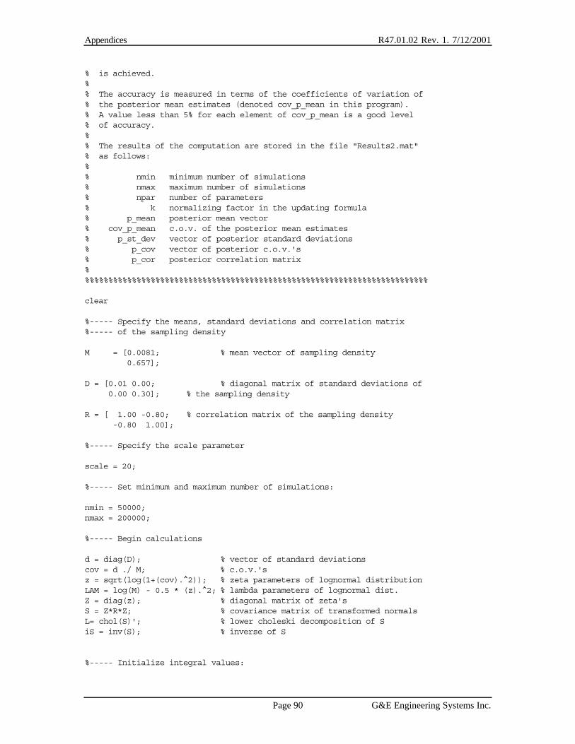
Appendices R47.01.02 Rev. 1. 7/12/2001


% is achieved.%% The accuracy is measured in terms of the coefficients of variation of% the posterior mean estimates (denoted cov_p_mean in this program).% A value less than 5% for each element of cov_p_mean is a good level% of accuracy.%% The results of the computation are stored in the file "Results2.mat"% as follows:%% nmin minimum number of simulations% nmax maximum number of simulations% npar number of parameters% k normalizing factor in the updating formula% p_mean posterior mean vector% cov_p_mean c.o.v. of the posterior mean estimates% p_st_dev vector of posterior standard deviations% p_cov vector of posterior c.o.v.'s% p_cor posterior correlation matrix%%%%%%%%%%%%%%%%%%%%%%%%%%%%%%%%%%%%%%%%%%%%%%%%%%%%%%%%%%%%%%%%%%%%%%%%%%

clear

%----- Specify the means, standard deviations and correlation matrix%----- of the sampling density

M = [0.0081; % mean vector of sampling density 0.657];

D = [0.01 0.00; % diagonal matrix of standard deviations of 0.00 0.30]; % the sampling density

R = [ 1.00 -0.80; % correlation matrix of the sampling density -0.80 1.00];

%----- Specify the scale parameter

scale = 20;

%----- Set minimum and maximum number of simulations:

nmin = 50000;nmax = 200000;

%----- Begin calculations

d = diag(D); % vector of standard deviationscov = d ./ M; % c.o.v.'sz = sqrt(log(1+(cov).^2)); % zeta parameters of lognormal distributionLAM = log(M) - 0.5 * (z).^2; % lambda parameters of lognormal dist.Z = diag(z); % diagonal matrix of zeta'sS = Z*R*Z; % covariance matrix of transformed normalsL= chol(S)'; % lower choleski decomposition of SiS = inv(S); % inverse of S

%----- Initialize integral values:

Appendices R47.01.02 Rev. 1. 7/12/2001


I1 = 0;I2 = 0;I3 = 0;I4 = 0;

npar = length(M); % number of parametersi_counter = 0;flag = 1;constant = 1/( (6.28318531)^(npar/2) * sqrt(det(S)) );

%----- Begin importance sampling:

for i = 1:nmax

%-- simulate standard normal random variables;u = random('Normal',0,1,npar,1);theta = exp( LAM + L*u); % simulated lognormal theta's

%-- define three kernelsK1 = 1;% this is for computing the normalizing constant k

K2 = theta; % this is for computing the meanK3 = theta*theta'; % this is for computing the mean squares

%-- compute the scaled likelihhod function lhood = exp(Loglhood2(theta)+scale);

%--- compute the prior distribution (non-informative): p = 1/(theta(1)*theta(2));

%--- compute the sampling probability densityh = constant * exp(-0.5*(log(theta)-LAM)'*iS*(log(theta)-LAM));h = h/(theta(1)*theta(2));

%--- compute (kernel*likelihood*prior)/sampling-density:I1 = I1 + K1*lhood*p/h;I2 = I2 + K2*lhood*p/h;I3 = I3 + K3*lhood*p/h;

I4 = I4 + (K2*lhood*p/h).^2; % this is for computing cov_p_mean

%--- reciprocal of the normalizing constantk = I1/i;

%--- posterior mean and its c.o.v.p_mean = I2/I1;cov_p_mean = sqrt(( 1/i*(I4/(k^2*i)-(I2/(k*i)).^2) ))./abs(p_mean);

%--- posterior covariance matrixp_cov = I3/I1 - p_mean*p_mean';

% check if c.o.v is <= 0.05 for all the posterior means, but% make sure that at least nmin simulations are performed.

% flag = 0 means that convergence has been achieved. i_counter = i_counter+1; if max(cov_p_mean) <= 0.05 & i_counter>nmin flag = 0; break end

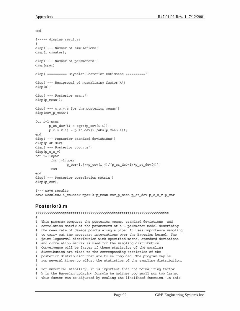
Appendices R47.01.02 Rev. 1. 7/12/2001


end

%----- display results:%disp('--- Number of simulations')disp(i_counter);

disp('--- Number of parameters')disp(npar)

disp('========== Bayesian Posterior Estimates ==========')

disp('--- Reciprocal of normalizing factor k')disp(k);

disp('--- Posterior means')disp(p_mean');

disp('--- c.o.v.s for the posterior means')disp(cov_p_mean')

for i=1:npar p_st_dev(i) = sqrt(p_cov(i,i)); p_c_o_v(i) = p_st_dev(i)/abs(p_mean(i));enddisp('--- Posterior standard deviations')disp(p_st_dev)disp('--- Posterior c.o.v.s')disp(p_c_o_v)for i=1:npar for j=1:npar p_cor(i,j)=p_cov(i,j)/(p_st_dev(i)*p_st_dev(j)); endenddisp('--- Posterior correlation matrix')disp(p_cor);

%--- save resultssave Results2 i_counter npar k p_mean cov_p_mean p_st_dev p_c_o_v p_cor

Posterior3.m%%%%%%%%%%%%%%%%%%%%%%%%%%%%%%%%%%%%%%%%%%%%%%%%%%%%%%%%%%%%%%%%%%%%%% This program computes the posterior means, standard deviations and% correlation matrix of the parameters of a 3-parameter model describing% the mean rate of damage points along a pipe. It uses importance sampling% to carry out the necessary integrations over the Bayesian kernel. The% joint lognormal distribution with specified means, standard deviations% and correlation matrix is used for the sampling distribution.% Convergence will be faster if these statistics of the sampling% distribution are close to the corresponding statistics of the% posterior distribution that are to be computed. The program may be% run several times to adjust the statistics of the sampling distribution.%% For numerical stability, it is important that the normalizing factor% k in the Bayesian updating formula be neither too small nor too large.% This factor can be adjusted by scaling the likelihood function. In this

Appendices R47.01.02 Rev. 1. 7/12/2001


% program this is done by adjusting the "scale" parameter.%% Run the program with trial estimates of the means, standard deviation% and correlation matrix of the sampling density, and of the scale% parameter. This will give a first estimate of the reciprocal of the% normalizing factor k and the posterior statistics of the parameters.% Make sure that the sampling density has sufficiently large standard% deviations (no smaller than the posterior standard deviations estimated).% Use the first posterior estimates as the new means, standard deviations% and correlation matrix of the sampling distribution and adjust the% scale parameter (decrease it if k is too large, increase it if k is too% small). Run the program again to obtain a second set of posterior estimates.% Repeat this process until sufficient accuracy in the posterior estimates% is achieved.%% The accuracy is measured in terms of the coefficients of variation of% the posterior mean estimates (denoted cov_p_mean in this program).% A value less than 5% for each element of cov_p_mean is a good level% of accuracy.%% The results of the computation are stored in the file "Results3.mat"% as follows:%% nmin minimum number of simulations% nmax maximum number of simulations% npar number of parameters% k normalizing factor in the updating formula% p_mean posterior mean vector% cov_p_mean c.o.v. of the posterior mean estimates% p_st_dev vector of posterior standard deviations% p_cov vector of posterior c.o.v.'s% p_cor posterior correlation matrix%%%%%%%%%%%%%%%%%%%%%%%%%%%%%%%%%%%%%%%%%%%%%%%%%%%%%%%%%%%%%%%%%%%%%%%%%%

clear

%----- Specify the means, standard deviations and correlation matrix%----- of the sampling density

M = [0.06; % mean vector of sampling density 0.8; 1.5];

D = [0.03 0.00 0.00; % diagonal matrix of standard deviations of 0.00 0.06 0.00; % the sampling density 0.00 0.00 0.14];

R = [ 1.00 -0.60 0.70; % correlation matrix of the sampling density -0.60 1.00 0.00; 0.70 0.00 1.00];

%----- Specify the scale parameter

scale = 310;

%----- Set minimum and maximum number of simulations:

Appendices R47.01.02 Rev. 1. 7/12/2001


nmin = 50000;nmax = 200000;

%----- Begin calculations

d = diag(D); % vector of standard deviationscov = d ./ M; % c.o.v.'sz = sqrt(log(1+(cov).^2)); % zeta parameters of lognormal distributionLAM = log(M) - 0.5 * (z).^2; % lambda parameters of lognormal dist.Z = diag(z); % diagonal matrix of zeta'sS = Z*R*Z; % covariance matrix of transformed normalsL= chol(S)'; % lower choleski decomposition of SiS = inv(S); % inverse of S

%----- Initialize integral values:I1 = 0;I2 = 0;I3 = 0;I4 = 0;

npar = length(M); % number of parametersi_counter = 0;flag = 1;constant = 1/( (6.28318531)^(npar/2) * sqrt(det(S)) );

%----- Begin importance sampling:

for i = 1:nmax

%-- simulate standard normal random variables;u = random('Normal',0,1,npar,1);theta = exp( LAM + L*u); % simulated lognormal theta's

%-- define three kernelsK1 = 1;% this is for computing the normalizing constant k

K2 = theta; % this is for computing the meanK3 = theta*theta'; % this is for computing the mean squares

%-- compute the scaled likelihhod function lhood = exp(Loglhood3(theta)+scale);

%--- compute the prior distribution (non-informative): p = 1/(theta(1)*theta(2)*theta(3));

%--- compute the sampling probability densityh = constant * exp(-0.5*(log(theta)-LAM)'*iS*(log(theta)-LAM));h = h/(theta(1)*theta(2)*theta(3));

%--- compute (kernel*likelihood*prior)/sampling-density:I1 = I1 + K1*lhood*p/h;I2 = I2 + K2*lhood*p/h;I3 = I3 + K3*lhood*p/h;

I4 = I4 + (K2*lhood*p/h).^2; % this is for computing cov_p_mean

%--- reciprocal of normalizing constantk = I1/i;

Appendices R47.01.02 Rev. 1. 7/12/2001


%--- posterior mean and its c.o.v.p_mean = I2/I1;cov_p_mean = sqrt(( 1/i*(I4/(k^2*i)-(I2/(k*i)).^2) ))./abs(p_mean);

%--- posterior covariance matrixp_cov = I3/I1 - p_mean*p_mean';

% check if c.o.v is <= 0.05 for all the posterior means, but% make sure that at least nmin simulations are performed.

% flag = 0 means that convergence has been achieved. i_counter = i_counter+1; if max(cov_p_mean) <= 0.05 & i_counter>nmin flag = 0; break endend

%----- display results:%disp('--- Number of simulations')disp(i_counter);

disp('--- Number of parameters')disp(npar)

disp('========== Bayesian Posterior Estimates ==========')

disp('--- Reciprocal of normalizing factor k')disp(k);

disp('--- Posterior means')disp(p_mean');

disp('--- c.o.v.s for the posterior means')disp(cov_p_mean')

for i=1:npar p_st_dev(i) = sqrt(p_cov(i,i)); p_c_o_v(i) = p_st_dev(i)/abs(p_mean(i));enddisp('--- Posterior standard deviations')disp(p_st_dev)disp('--- Posterior c.o.v.s')disp(p_c_o_v)for i=1:npar for j=1:npar p_cor(i,j)=p_cov(i,j)/(p_st_dev(i)*p_st_dev(j)); endenddisp('--- Posterior correlation matrix')disp(p_cor);

%--- save resultssave Results3 i_counter npar k p_mean cov_p_mean p_st_dev p_c_o_v p_cor

Loglhood2.m

% FUNCTION STATEMENT

Appendices R47.01.02 Rev. 1. 7/12/2001


% Loglhood2 is a string containing the name of a function that computes% the logarithm of the likelihood function for the 2-parameter model% of the mean rate of pipe damage. This function reads the necessary% data stored in array "x" from the file named "Data2.m".

% ** VARIABLE DESCRIPTION **% theta = model parameters;% Loglhood2 = logarithm of the likelihood function.

function[Loglhood2] = Loglhood2(theta)

% load data stored in array x:

Data2

[nobsrv] = size(x);a = theta(1);b = theta(2);

% Log-likelihood calculationLoglhood2 = 0;

for i = 1 : nobsrv

Vi = x(i,1); % PGV in cm/sLi = x(i,2); % Pipe length in kmNi = x(i,4); % Number of damage points

lambdaL = a * (Vi^b) * Li;if Ni==0LogP = -lambdaL;elseif Ni>0LogP = Ni*log(lambdaL) - log(factorial(Ni)) - lambdaL;end

Loglhood2 = Loglhood2 + LogP;

end

Loglhood3.m

% FUNCTION STATEMENT% Loglhood3 is a string containing the name of a function that computes% the logarithm of the likelihood function for the 3-parameter model% of the mean rate of pipe damage. This function reads the necessary% data stored in array "x" from the file named "Data3.m".

% ** VARIABLE DESCRIPTION **% theta = model parameters;% Loglhood3 = logarithm of the likelihood function.

function[Loglhood3] = Loglhood3(theta)

% load data stored in array x:

Data3

[nobsrv] = size(x);a = theta(1);b = theta(2);

Appendices R47.01.02 Rev. 1. 7/12/2001


c = theta(3);

% Log-likelihood calculationLoglhood3 = 0;

for i = 1 : nobsrv

Vi = x(i,1); % PGV in cm/sLi = x(i,2); % Pipe length in kmDi = x(i,3); % Pipe diameter in inchesNi = x(i,4); % Number of damage points

lambdaL = a * (Vi^b) * (Di^(-c)) * Li;if Ni==0LogP = -lambdaL;elseif Ni>0LogP = Ni*log(lambdaL) - log(factorial(Ni)) - lambdaL;end

Loglhood3 = Loglhood3 + LogP;

end

Data2.m

% This file contains failure data on pipes damaged in past earthquakes.% This data is for Ductile Iron pipes and was collected by O'Rourke% and Jeon after the Northridge 1994 earthquake.%% V = Peak Ground Velocity, cm/s% L = Pipe segment length, km% D = Range of pipe diameters (not used in the calculation)% N = Number of damage points in the pipe segment.

% V L D Nx = [ 5 42.2 420 0; 15 116.7 420 1; 25 92.7 420 6; 35 40.3 420 2; 45 32.2 420 3; 55 18.1 420 1; 65 12.8 420 4; 75 7.5 420 2; 85 5.3 420 1; 95 16.1 420 1; 105 7.4 420 0; 115 15.6 420 1; 125 5.8 420 0; 135 5.4 420 0; 145 5.7 420 0; 155 5.4 420 1; 165 3.3 420 1];

Appendices R47.01.02 Rev. 1. 7/12/2001


Data3.m% This file contains failure data on pipes damaged in past earthquakes.% and Jeon after the Northridge 1994 earthquake.% This data is for Cast Iron pipes with diameters 4-12 inches.%% V = Peak Ground Velocity, cm/s% L = Pipe segment length, km% D = Pipe diameter, in% N = Number of damage points in the pipe segment.%% V L D N

x = [ 5 33.8 4 0; 15 263.8 4 7; 25 387.2 4 64; 35 129.5 4 29; 45 52.3 4 24; 55 23.3 4 18; 65 22.4 4 15; 75 9.4 4 6; 85 10.4 4 2; 95 8.0 4 0; 105 9.9 4 0; 115 9.2 4 0; 125 7.5 4 0; 135 4.8 4 0; 145 3.3 4 4; 155 3.6 4 0; 165 4.1 4 5; 5 126.5 6 0; 15 768.7 6 24; 25 878.8 6 66; 35 536.9 6 58; 45 427.7 6 22; 55 276.0 6 23; 65 195.5 6 45; 75 84.7 6 21; 85 72.4 6 10; 95 48.2 6 1; 105 53.1 6 1; 115 47.7 6 3; 125 40.4 6 4; 135 28.5 6 0; 145 33.9 6 2; 155 30.9 6 9; 165 32.0 6 19; 5 47.5 8 0; 15 379.5 8 5; 25 574.1 8 25; 35 298.5 8 14; 45 230.5 8 9; 55 140.0 8 10; 65 90.9 8 18; 75 62.0 8 11; 85 42.1 8 11; 95 21.0 8 1; 105 23.1 8 1;

Appendices R47.01.02 Rev. 1. 7/12/2001


115 22.8 8 2; 125 17.0 8 1; 135 24.4 8 2; 145 19.8 8 3; 155 15.6 8 5; 165 24.8 8 20; 5 3.7 10 0; 15 16.5 10 0; 25 30.6 10 3; 35 3.0 10 0; 5 23.3 12 0; 15 193.0 12 6; 25 263.0 12 7; 35 125.0 12 8; 45 84.7 12 4; 55 56.0 12 5; 65 34.9 12 7; 75 19.7 12 1; 85 8.4 12 1; 95 10.7 12 0; 105 7.9 12 0; 115 4.0 12 0; 125 6.4 12 1; 135 7.5 12 0; 145 4.6 12 1; 155 6.8 12 2; 165 5.4 12 0];

Data_AC.m% This file contains failure data on pipes damaged in past earthquakes.% This data is for Asbestos Cement pipes and was collected by O'Rourke% and Jeon after the Northridge 1994 earthquake.%% V = Peak Ground Velocity, cm/s% L = Pipe segment length, km% D = Range of pipe diameters, in (not used in the analysis)% N = Number of damage points in the pipe segment.%% V L D N

x = [ 5 157.3 412 0; 15 307.9 412 2; 25 235.5 412 15; 35 117.7 412 2; 45 37.8 412 0; 55 34.1 412 0; 65 24.4 412 7; 75 10.9 412 0; 85 3.0 412 0; 95 1.2 412 0; 105 4.8 412 0; 115 1.6 412 0; 125 3.9 412 0; 135 7.2 412 0; 145 5.0 412 0; 155 5.8 412 0; 165 3.5 412 0];

Appendices R47.01.02 Rev. 1. 7/12/2001


Data_CI_16_24.m% This file contains failure data on pipes damaged in past earthquakes.% This data is for Cast Iron pipes and was collected by O'Rourke% and Jeon after the Northridge 1994 earthquake.%% V = Peak Ground Velocity, cm/s% L = Pipe segment length, km% D = Range of pipe diameters, in (not used in the analysis)% N = Number of damage points in the pipe segment.%% V L D N

x = [ 5 15.9 1624 0; 15 67.6 1624 2; 25 59.8 1624 1; 35 27.2 1624 2; 45 9.8 1624 0; 55 6.9 1624 0; 65 12.6 1624 2; 75 2.8 1624 0; 85 6.8 1624 1; 95 4.3 1624 0; 105 2.0 1624 0; 115 2.9 1624 0; 125 4.9 1624 0; 135 6.2 1624 0; 145 2.7 1624 0; 155 2.9 1624 0; 165 0.0

G.12 ReferencesAng, A. H-S., and W-H. Tang. Probability concepts in engineering planning and design,vol. I - basic principles. John Wiley & Sons, New York, N.Y, 1975.

Box, G.E.P., and Tiao, G.C. Bayesian Inference in Statistical Analysis, Addison-Wesley,Reading, Mass, 1992.


PGV

cm / secL n L n L n L n L n L n L n L n L n

5 33.8 0 126.5 0 47.5 0 3.7 0 23.3 0 7.8 0 0.2 0 8 01 5 263.8 7 768.7 2 4 379.5 5 16.5 0 1 9 3 6 32.4 2 2.3 0 3 2 0 0.8 02 5 387.2 6 4 878.8 6 6 574.1 2 5 30.6 3 2 6 3 7 43.8 0 4.4 1 1 1 0 0.5 03 5 129.5 2 9 536.9 5 8 298.5 1 4 3 0 1 2 5 8 19.7 1 0.2 0 5.3 1 1.9 04 5 52.3 2 4 427.7 2 2 230.5 9 84.7 4 9.2 0 0.6 05 5 23.3 1 8 2 7 6 2 3 1 4 0 1 0 5 6 5 6.9 06 5 22.4 1 5 195.5 4 5 90.9 1 8 34.9 7 11.9 2 0.7 07 5 9.4 6 84.7 2 1 6 2 1 1 19.7 1 2.3 0 0.6 08 5 10.4 2 72.4 1 0 42.1 1 1 8.4 1 3.9 0 2.9 19 5 8 0 48.2 1 2 1 1 10.7 0 3 0 1.2 0

1 0 5 9.9 0 53.1 1 23.1 1 7.9 0 1.8 0 0.2 01 1 5 9.2 0 47.9 3 22.8 2 4 0 2.4 0 0.4 01 2 5 7.5 0 40.4 4 1 7 1 6.4 1 4.3 0 0.6 01 3 5 4.8 0 28.5 0 24.4 2 7.5 0 5 0 1.2 01 4 5 3.3 3 33.9 2 19.8 3 4.6 1 2.7 01 5 5 3.6 0 30.9 9 15.6 5 6.8 2 2.1 0 0.9 01 6 5 4.1 5 3 2 1 9 24.8 2 0 5.4 0

Total 982.5 1 7 3 3682.1 3 0 8 2033.6 1 3 8 53.8 3 861.3 4 3 159.2 5 7.1 1 65.6 2 3.2 0

NotesL = length of pipeline in km, within the specified PGV binn = number of repairs See Section G.1 for further description of the data

2 4Pipe Diameter, Inches

1 2 1 6 1 8 2 04 6 8 1 0

Table G-1. Cast Iron Pipe Damage, 1994 Northridge Earthquake, LADWP


PGV

cm / secL n L n L n L n L n L n

5 0.9 0 19.9 0 11.6 0 5.3 0 3.4 0 1.1 01 5 2.2 0 53.2 1 32.4 0 21.4 0 4.6 0 2.9 02 5 2.5 1 47.5 5 3 3 0 8 0 1.7 03 5 1.3 1 1 6 0 12.8 1 6.5 0 2.3 0 1.4 04 5 1.7 1 10.8 1 10.6 1 8.4 0 0.7 05 5 2.1 0 6.2 1 8.5 0 1.3 0 0 06 5 2.1 0 5.6 3 3.4 1 1.4 0 0.2 0 0.2 07 5 1.3 1 1.7 0 2.3 1 2.3 08 5 0.3 0 2 1 0.4 0 2.6 09 5 2.6 0 6.2 0 4.5 0 2.7 0 0.1 1

105 0.6 0 2.8 0 2.1 0 0.2 0 1.7 0115 1.5 0 3.9 0 6.5 0 2.2 1 1.4 0 0.2 0125 0.8 0 2.5 0 1.3 0 0.7 0 0.6 0135 0.5 0 2.7 0 0.4 0 0.7 0 0.8 0 0.3 0145 0.3 0 3.2 0 1.4 0 0.7 0 0.1 0155 4.3 0 0.1 1 0.7 0 0.3 0165 2.6 1 0.7 0

Total 20.7 4 191.1 1 3 131.3 5 65.1 1 17.9 1 6.8 0


Pipeline Diameter, Inches1 2 1 6 2 04 6 8

Table G-2. Ductile Iron Pipe Damage, 1994 Northridge Earthquake, LADWP


PGV

cm / secL n L n L n L n L n

5 9.5 0 79.3 0 53.4 0 15.1 01 5 14.1 0 180.5 2 88.1 0 1.9 0 23.2 02 5 12.5 6 129.7 7 82.1 2 11.2 03 5 8 0 73.2 1 32.2 1 4.3 04 5 1.1 0 22.6 0 13.1 0 1 05 5 2.8 0 25.1 0 5.4 0 0.7 06 5 2.6 7 17.6 0 3.9 0 0.2 07 5 2.4 0 7 0 1.5 08 5 0.7 0 2.1 0 0.1 09 5 0.3 0 0.9 0

105 0.5 0 3.2 0 1.2 0115 0.2 0 1 0 0.4 0125 0.3 0 3.4 0 0.1 0135 0.6 0 5.5 0 1.1 0145 0.2 0 3 0 1.8 0155 0.5 0 3.4 0 1.9 0165 0.1 0 2.6 0 0.9 0

Total 56.4 1 3 560.1 1 0 287.2 3 1.9 0 55.7 0


Pipeline Diameter, Inches1 0 1 24 6 8

Table G-3. Asbestos Cement Pipe Damage, 1994 Northridge Earthquake, LADWP

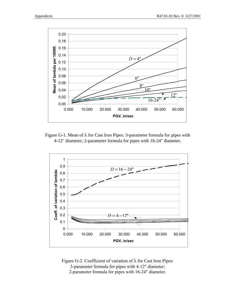
Appendices R47.01.02 Rev. 0. 3/27/2001

Figure G-1. Mean of λ for Cast Iron Pipes: 3-parameter formula for pipes with4-12" diameter; 2-parameter formula for pipes with 16-24" diameter.

Figure G-2. Coefficient of variation of λ for Cast Iron Pipes:3-parameter formula for pipes with 4-12" diameter;2-parameter formula for pipes with 16-24" diameter.

0.00

0.02

0.04

0.06

0.08

0.10

0.12

0.14

0.16

0.18

0.20

0.000 10.000 20.000 30.000 40.000 50.000 60.000

PGV, in/sec

Mea

n o

f la

mb

da

per

100

0ft

"4=D

"6

"8"10

"1216-24″

0

0.1

0.2

0.3

0.4

0.5

0.6

0.7

0.8

0.9

1

0.000 10.000 20.000 30.000 40.000 50.000 60.000

PGV, in/sec

Co

eff.

of

vari

atio

n o

f la

mb

da

"124 −=D

"2416 −=D

Appendices R47.01.02 Rev. 0. 3/27/2001

Figure G-3. Mean of λ for Ductile Iron pipes with 4-20" Diameter.

Figure G-4. Coefficient of Variation of λ for Ductile Iron Pipes with 4-20" Diameter.

0.00

0.01

0.02

0.03

0.04

0.05

0.06

0.07

0.08

0 10 20 30 40 50 60

PGV, in/sec

Mea

n o

f la

mb

da

per

100

0ft

0

0.1

0.2

0.3

0.4

0.5

0.6

0.7

0.8

0 10 20 30 40 50 60

PGV, in/sec

Co

eff.

of

vari

atio

n o

f la

mb

da

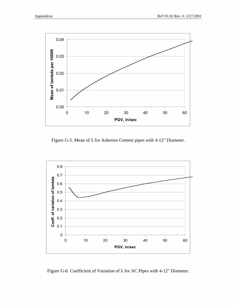
Appendices R47.01.02 Rev. 0. 3/27/2001

Figure G-5. Mean of λ for Asbestos Cement pipes with 4-12" Diameter.

Figure G-6. Coefficient of Variation of λ for AC Pipes with 4-12" Diameter.

0.00

0.01

0.02

0.03

0.04

0 10 20 30 40 50 60

PGV, in/sec

Mea

n o

f la

mb

da

per

100

0ft

0

0.1

0.2

0.3

0.4

0.5

0.6

0.7

0.8

0 10 20 30 40 50 60

PGV, in/sec

Coe

ff. o

f var

iatio

n of

lam

bda

Appendices R47.01.02 Rev. 0. 3/27/2001

Figure G-7. Comparison of Mean of λ for Pipes of Different Material and Diameter.

Figure G-8. Comparison of C.O.V. of λ for Pipes of Different Material and Diameter.

0.00

0.02

0.04

0.06

0.08

0.10

0.12

0.14

0.16

0.18

0.20

0 10 20 30 40 50 60

PGV, in/sec

Mea

n o

f la

mb

da

per

100

0ft

0

0.1

0.2

0.3

0.4

0.5

0.6

0.7

0.8

0.9

1

0 10 20 30 40 50 60

PGV, in/sec

Co

eff.

of

vari

atio

n o

f la

mb

da

CI pipesDI pipesAC pipes

CI pipesDI pipesAC pipes

CI pipe with "4=D

CI pipe with "2416 −=D



seismic fragility formulations for water systems · seismic fragility formulations for water...

Documents