seismic hazard and seismic risk analysis - civil engineering
TRANSCRIPT

FEMA 451B Topic 15-3 Notes Seismic Hazard Analysis 15-3 - 1
Hazard & Risk Analysis 15-3 - 1Instructional Material Complementing FEMA 451, Design Examples
SEISMIC HAZARD AND SEISMIC RISK ANALYSIS
• Seismotectonics
• Fault mechanics
• Ground motion considerations for design
• Deterministic and probabilistic analysis• Estimation of ground motions • Scaling of ground motions and design
and analysis tools (i.e., NONLIN)
Note that many of the graphics used for this material were obtained from the U.S. Geological Survey (USGS) and other U.S. government sources. These graphics are in the public domain and not subject to copyright; however, appropriate credit is and should be given for such reproduced graphics.
FEMA 451B Topic 15-3 Notes Seismic Hazard Analysis 15-3 - 2
Hazard & Risk Analysis 15-3 - 2Instructional Material Complementing FEMA 451, Design Examples
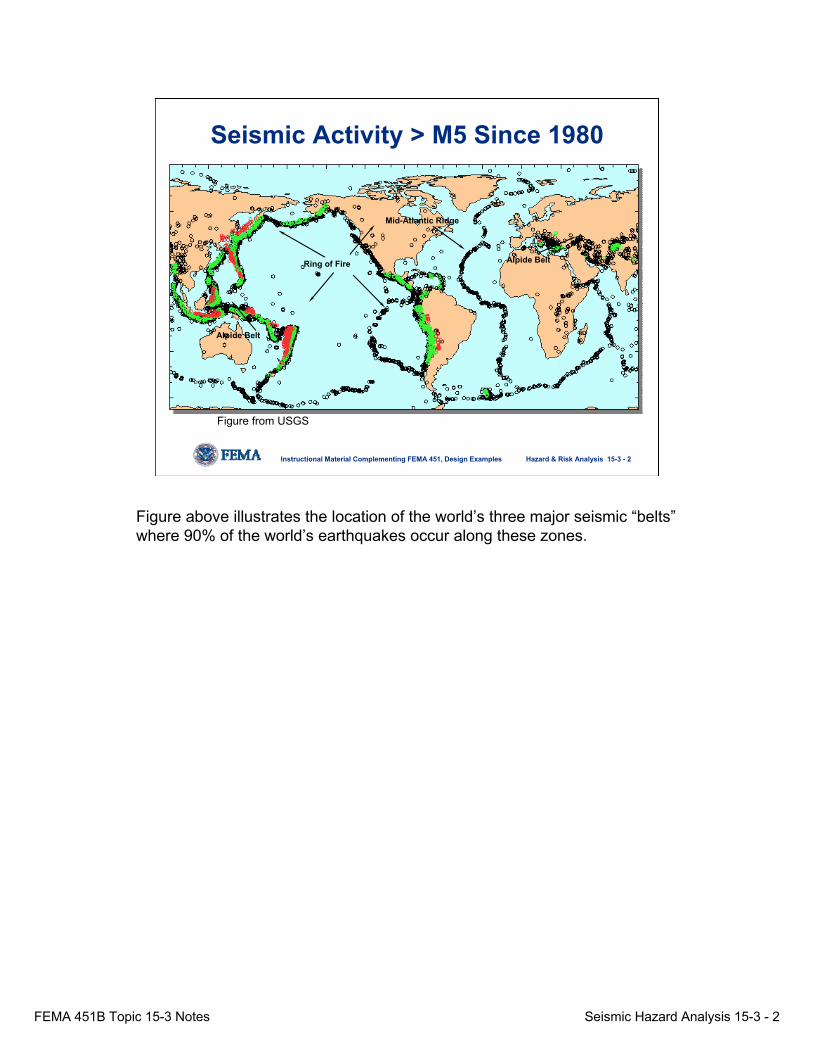
Seismic Activity > M5 Since 1980
Ring of Fire
Mid-Atlantic Ridge
Alpide Belt
Alpide Belt
Figure from USGS
Figure above illustrates the location of the world’s three major seismic “belts”where 90% of the world’s earthquakes occur along these zones.

FEMA 451B Topic 15-3 Notes Seismic Hazard Analysis 15-3 - 3
Hazard & Risk Analysis 15-3 - 3Instructional Material Complementing FEMA 451, Design Examples
Crustal Plate Boundaries
Figure from USGS
Major plates and plate boundaries are shown. The existence of plates were first proposed around 1920 by A. Wegner, but it was not until the 1960s, with greatly improved seismic monitoring equipment and a marked increase in ocean floor research, that data revealed irrefutably the existence of a series of large plates. The locations of the earthquakes shown on the previous slide roughly delineate the boundaries of the major plates.
FEMA 451B Topic 15-3 Notes Seismic Hazard Analysis 15-3 - 4
Hazard & Risk Analysis 15-3 - 4Instructional Material Complementing FEMA 451, Design Examples
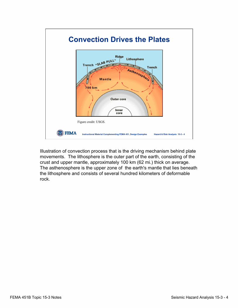
Convection Drives the Plates
Figure credit: USGS.
Illustration of convection process that is the driving mechanism behind plate movements. The lithosphere is the outer part of the earth, consisting of the crust and upper mantle, approximately 100 km (62 mi.) thick on average. The asthenosphere is the upper zone of the earth's mantle that lies beneath the lithosphere and consists of several hundred kilometers of deformable rock.

FEMA 451B Topic 15-3 Notes Seismic Hazard Analysis 15-3 - 5
Hazard & Risk Analysis 15-3 - 5Instructional Material Complementing FEMA 451, Design Examples
Oceanic and Crustal Plates
thin lithosphereunder oceans ( ~ 50 km)
asthenosphere~ 500 km
Continental Plate (light)
Oceanic Plate (heavy)
oceanic crust
solid mantle
partially melted mantle
continental crust
thick lithosphere beneath continents(~ 100 km)
Depiction of typical relationship between the lithosphere and asthenosphereas well as difference between heavy oceanic crust and lighter continental crust. Lighter continental crust tends to “float” and heavy oceanic crust sinks or subducts below lighter continental crust when they collide. Continental crust is typically composed of silicic or granitic rocks with lighter minerals such as quartz and feldspar whereas oceanic crust is colder and denser and typically consists of mafic or basaltic rock rich in heavy mineral such as pyroxene or olivine.

FEMA 451B Topic 15-3 Notes Seismic Hazard Analysis 15-3 - 6
Hazard & Risk Analysis 15-3 - 6Instructional Material Complementing FEMA 451, Design Examples
Continental-Continental Collision(orogeny)
Figure credit: USGS.
Collisions of continental plates results in mountain building (orogeny).
FEMA 451B Topic 15-3 Notes Seismic Hazard Analysis 15-3 - 7
Hazard & Risk Analysis 15-3 - 7Instructional Material Complementing FEMA 451, Design Examples
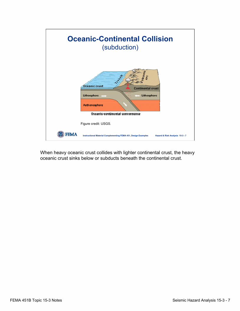
Oceanic-Continental Collision(subduction)
Figure credit: USGS.
When heavy oceanic crust collides with lighter continental crust, the heavy oceanic crust sinks below or subducts beneath the continental crust.
FEMA 451B Topic 15-3 Notes Seismic Hazard Analysis 15-3 - 8
Hazard & Risk Analysis 15-3 - 8Instructional Material Complementing FEMA 451, Design Examples
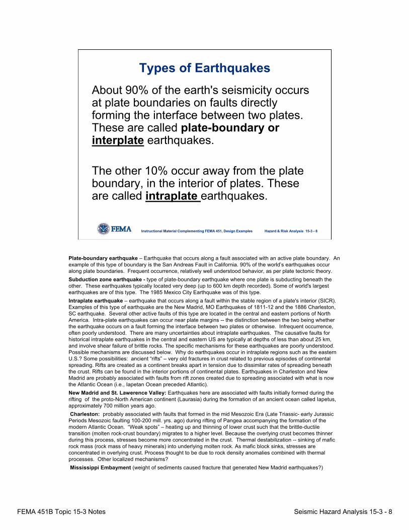
Types of EarthquakesAbout 90% of the earth's seismicity occurs at plate boundaries on faults directly forming the interface between two plates. These are called plate-boundary or interplate earthquakes.
The other 10% occur away from the plate boundary, in the interior of plates. These are called intraplate earthquakes.
Plate-boundary earthquake – Earthquake that occurs along a fault associated with an active plate boundary. An example of this type of boundary is the San Andreas Fault in California. 90% of the world’s earthquakes occur along plate boundaries. Frequent occurrence, relatively well understood behavior, as per plate tectonic theory.Subduction zone earthquake - type of plate-boundary earthquake where one plate is subducting beneath the other. These earthquakes typically located very deep (up to 600 km depth recorded). Some of world's largest earthquakes are of this type. The 1985 Mexico City Earthquake was of this type. Intraplate earthquake – earthquake that occurs along a fault within the stable region of a plate's interior (SICR). Examples of this type of earthquake are the New Madrid, MO Earthquakes of 1811-12 and the 1886 Charleston, SC earthquake. Several other active faults of this type are located in the central and eastern portions of North America. Intra-plate earthquakes can occur near plate margins -- the distinction between the two being whether the earthquake occurs on a fault forming the interface between two plates or otherwise. Infrequent occurrence, often poorly understood. There are many uncertainties about intraplate earthquakes. The causative faults for historical intraplate earthquakes in the central and eastern US are typically at depths of less than about 25 km, and involve shear failure of brittle rocks. The specific mechanisms for these earthquakes are poorly understood. Possible mechanisms are discussed below. Why do earthquakes occur in intraplate regions such as the eastern U.S.? Some possibilities: ancient “rifts” – very old fractures in crust related to previous episodes of continental spreading. Rifts are created as a continent breaks apart in tension due to dissimilar rates of spreading beneath the crust. Rifts can be found in the interior portions of continental plates. Earthquakes in Charleston and New Madrid are probably associated with faults from rift zones created due to spreading associated with what is now the Atlantic Ocean (i.e., Iapetan Ocean preceded Atlantic). New Madrid and St. Lawerence Valley: Earthquakes here are associated with faults initially formed during the rifting of the proto-North American continent (Laurasia) during the formation of an ancient ocean called Iapetus, approximately 700 million years ago.Charleston: probably associated with faults that formed in the mid Mesozoic Era (Late Triassic- early Jurassic
Periods Mesozoic faulting 100-200 mill. yrs. ago) during rifting of Pangea accompanying the formation of the modern Atlantic Ocean. “Weak spots” – heating up and thinning of lower crust such that the brittle-ductile transition (molten rock-crust boundary) migrates to a higher level. Because the overlying crust becomes thinner during this process, stresses become more concentrated in the crust. Thermal destabilization -- sinking of mafic rock mass (rock mass of heavy minerals) into underlying molten rock. As mafic block sinks, stresses are concentrated in overlying crust. Process thought to be due to rock density anomalies combined with thermal processes. Other localized mechanisms?Mississippi Embayment (weight of sediments caused fracture that generated New Madrid earthquakes?)
FEMA 451B Topic 15-3 Notes Seismic Hazard Analysis 15-3 - 9
Hazard & Risk Analysis 15-3 - 9Instructional Material Complementing FEMA 451, Design Examples
Plate-boundary Earthquakes
A plate-boundary (interplate) earthquakeis an earthquake that occurs along a fault associated with an active plate boundary. An example of this type of boundary is the San Andreas Fault in California.
⇒ Frequent occurrence, relatively well understood behavior, as per plate tectonic theory.
Plate-boundary earthquake – Earthquake that occurs along a fault associated with an active plate boundary. An example of this type of boundary is the San Andreas Fault in California. 90% of the world’s earthquakes occur along plate boundaries.

FEMA 451B Topic 15-3 Notes Seismic Hazard Analysis 15-3 - 10
Hazard & Risk Analysis 15-3 - 10Instructional Material Complementing FEMA 451, Design Examples
San Andreas Fault – Well Known Plate Boundary
Photo courtesy of: USGS.
Slide shows the San Andreas Fault System. Note that there are at least two prominent fractures that can be seen. Thus, there are many smaller faults associated with he San Andreas Fault System as would be expected with two major plates meet. The San Andreas Fault involves mostly strike-slip type faulting movement.

FEMA 451B Topic 15-3 Notes Seismic Hazard Analysis 15-3 - 11
Hazard & Risk Analysis 15-3 - 11Instructional Material Complementing FEMA 451, Design Examples
Intraplate Earthquakes
An intraplate earthquake is an earthquake that occurs along a fault within the stable region of a plate's interior (SICR). Examples are the 1811-12 Madrid, MO earthquakes, the 1886 Charleston, South Carolina, earthquake, and, more recently, the Bhuj, India, earthquake in 2001.
⇒ Infrequent occurrence, poorly understood, difficult to study.
Intraplate earthquake – earthquake that occurs along a fault within the stable region of a plate's interior (SICR). Examples of this type of earthquake are the New Madrid, Missouri, earthquakes of 1811-12 and the 1886 Charleston, South Carolina, earthquake. Several other active faults of this type are located in the central and eastern portions of North America.
FEMA 451B Topic 15-3 Notes Seismic Hazard Analysis 15-3 - 12
Hazard & Risk Analysis 15-3 - 12Instructional Material Complementing FEMA 451, Design Examples
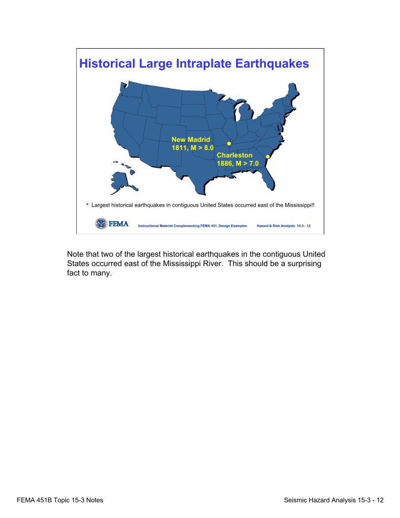
New Madrid 1811, M > 8.0
Charleston 1886, M > 7.0
Historical Large Intraplate Earthquakes
* Largest historical earthquakes in contiguous United States occurred east of the Mississippi!!
Note that two of the largest historical earthquakes in the contiguous United States occurred east of the Mississippi River. This should be a surprising fact to many.

FEMA 451B Topic 15-3 Notes Seismic Hazard Analysis 15-3 - 13
Hazard & Risk Analysis 15-3 - 13Instructional Material Complementing FEMA 451, Design Examples
Why Intraplate Earthquakes?
• Ancient “Rifts” – very old fractures in crust related to previous episodes of continental spreading.
• “Weak Spots” – heating up and thinning of lower crust such that the brittle-ductile transition (molten rock/crust boundary) migrates to a higher level. Because the overlying crust becomes thinner, stresses become more concentrated in the crust.
Rift zones from episodes of continental rifting (breaking of crust in tension basically) are associated with earthquakes in several intraplate regions, especially in the central and eastern United States (CEUS and EUS); however, other mechanisms such as weak spots are less definitive in terms of the occurrence of intraplate earthquakes.
FEMA 451B Topic 15-3 Notes Seismic Hazard Analysis 15-3 - 14
Hazard & Risk Analysis 15-3 - 14Instructional Material Complementing FEMA 451, Design Examples
Why Intraplate Earthquakes?
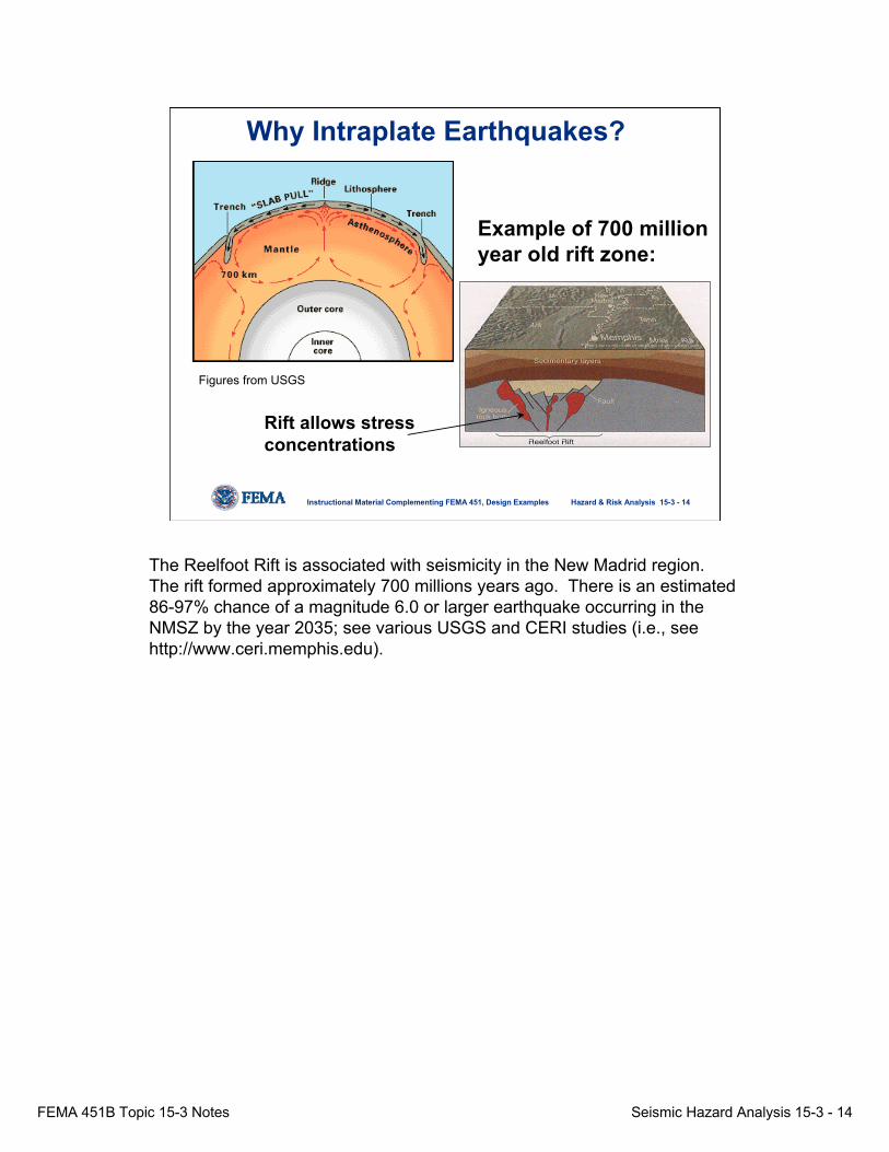
Example of 700 million year old rift zone:
Rift allows stress concentrations
Figures from USGS
The Reelfoot Rift is associated with seismicity in the New Madrid region. The rift formed approximately 700 millions years ago. There is an estimated 86-97% chance of a magnitude 6.0 or larger earthquake occurring in the NMSZ by the year 2035; see various USGS and CERI studies (i.e., see http://www.ceri.memphis.edu).
FEMA 451B Topic 15-3 Notes Seismic Hazard Analysis 15-3 - 15
Hazard & Risk Analysis 15-3 - 15Instructional Material Complementing FEMA 451, Design Examples
Why Intraplate Earthquakes?
• Thermal destabilization -- sinking of mafic rock mass (rock mass of heavy minerals) into underlying molten rock. As mafic block sinks, stresses are concentrated in overlying crust. Process thought to be due to rock density anomalies combined with thermal processes.
• Other localized mechanisms? (meteor impact craters, etc.)
Rift zones from episodes of continental rifting (breaking of crust in tension basically) are associated with earthquakes in several intraplate regions, especially in the central and eastern US; however, other mechanisms such as weak spots are less definitive in terms of the occurrence of intraplate earthquakes.

FEMA 451B Topic 15-3 Notes Seismic Hazard Analysis 15-3 - 16
Hazard & Risk Analysis 15-3 - 16Instructional Material Complementing FEMA 451, Design Examples
Pacific Plate
North AmericanPlate
Seismicity of North America
Figure credit: USGS.
Red data points in figure indicate locations of recorded earthquakes in 48 states. Map above represents earthquake activity over about a 20-year period and earthquakes shown are large enough to have been felt (> magnitude 4 or so). The map indicates that most US seismicity is located in the western states, but earthquake occur in many regions of the US, including the interior portions of the plate. In general, east of the Rockies, individual known faults and fault lines are unreliable guides to the likelihood of earthquakes. In California, a large earthquake can generally be associated with a particular fault because we have watched the fault break and offset the ground surface during the earthquake. In contrast, east of the Rockies things are less straightforward, because it is rare for earthquakes to break the ground surface. In particular, east of the Rockies, most known faults and fault lines do not appear to have anything to do with modern earthquakes. We don't know why. We do know that most earthquake locations cannot be measured very accurately east of the Rockies. Earthquakes typically occur several miles deep within the Earth. Their locations, including their depths, are usually uncertain by a mile or more. Although the larger faults extend from their fault lines downward deep into the Earth, their locations at earthquake depths are usually wholly unknown. The uncertain underground locations of earthquakes and faults make it terrifically hard to determine whether a particular earthquake occurred on a particular known fault. We also know that there are many faults hidden underground that are large enough to generate damaging earthquakes, but which are also too small to extend from earthquake depths all the way up to ground level where we have the best chance of seeing the faults. These hidden faults are likely to be at least as numerous as the faults we know about. Accordingly, an earthquake is as likely to occur on an unknown fault as on a known fault, if not more likely. The result of all this is that fault lines east of the Rockies are unreliable guides to where earthquakes are likely to occur. Accordingly, the best guide to earthquake hazard east of the Rockies is probably the earthquakes themselves. This doesn't mean that future earthquakes will occur exactly where past ones did, although that can happen. It means that future earthquakes are most likely to occur in the same general regions that had past earthquakes. Some future earthquakes are likely to occur far from past ones, in areas that have had few or no past earthquakes. However, these surprises are not too common. Most earthquakes tend to occur in the same general regions that are already known to have earthquakes.
FEMA 451B Topic 15-3 Notes Seismic Hazard Analysis 15-3 - 17
Hazard & Risk Analysis 15-3 - 17Instructional Material Complementing FEMA 451, Design Examples
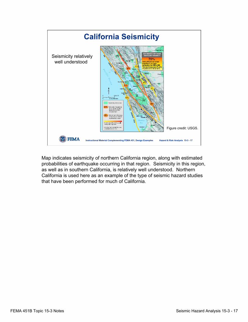
California Seismicity
Seismicity relatively well understood
Figure credit: USGS.
Map indicates seismicity of northern California region, along with estimated probabilities of earthquake occurring in that region. Seismicity in this region, as well as in southern California, is relatively well understood. Northern California is used here as an example of the type of seismic hazard studies that have been performed for much of California.

FEMA 451B Topic 15-3 Notes Seismic Hazard Analysis 15-3 - 18
Hazard & Risk Analysis 15-3 - 18Instructional Material Complementing FEMA 451, Design Examples
Pacific Northwest – Cascadia Subduction Zone
Ultimate magnitude potential?
Figure Credit: USGS
Although the seismic mechanism is relatively well understood forearthquakes in the Pacific Northwest – most are associated with the Cascadia Subduction Zone, there is still much debate as to how large earthquakes along this zone can be. More specifically, there is debate as to how strong ground shaking would be inland in the populated regions. Some have suggested the possibility of great earthquakes, exceeding magnitude 8. However recent studies have refuted these claims and do not suggest earthquake shaking from events this large during the last several thousand years.

FEMA 451B Topic 15-3 Notes Seismic Hazard Analysis 15-3 - 19
Hazard & Risk Analysis 15-3 - 19Instructional Material Complementing FEMA 451, Design Examples
Idaho, Utah, Wyoming
Recurring events along WasatchFault
Figure credit: USGS.
Figure illustrates paleo-evidence of recurring earthquakes along the Wasatch Fault. The dates of the earthquakes were determined frompaleoseismic investigations.

FEMA 451B Topic 15-3 Notes Seismic Hazard Analysis 15-3 - 20
Hazard & Risk Analysis 15-3 - 20Instructional Material Complementing FEMA 451, Design Examples
Central US Seismic Zones
• Who really knows for sure?
• The Reelfoot Rift is associated with many events in this region.
Figure credit: USGS.
Specific seismic mechanisms in the CEUS are not as well understood, but the Reelfoot Rift is known to be associated with many earthquakes in this region. (Rift zones from episodes of continental rifting (breaking of crust in tension basically) are associated with earthquakes in several intraplate regions, especially in the central and eastern US; however, other mechanisms such as weak spots are less definitive in terms of the occurrence of intraplate earthquakes).
FEMA 451B Topic 15-3 Notes Seismic Hazard Analysis 15-3 - 21
Hazard & Risk Analysis 15-3 - 21Instructional Material Complementing FEMA 451, Design Examples
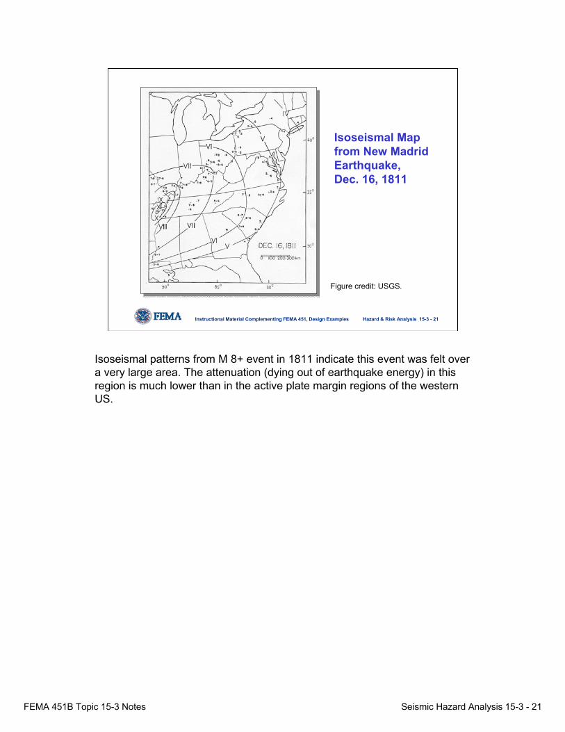
Isoseismal Mapfrom New MadridEarthquake,Dec. 16, 1811
Figure credit: USGS.
Isoseismal patterns from M 8+ event in 1811 indicate this event was felt over a very large area. The attenuation (dying out of earthquake energy) in this region is much lower than in the active plate margin regions of the western US.
FEMA 451B Topic 15-3 Notes Seismic Hazard Analysis 15-3 - 22
Hazard & Risk Analysis 15-3 - 22Instructional Material Complementing FEMA 451, Design Examples
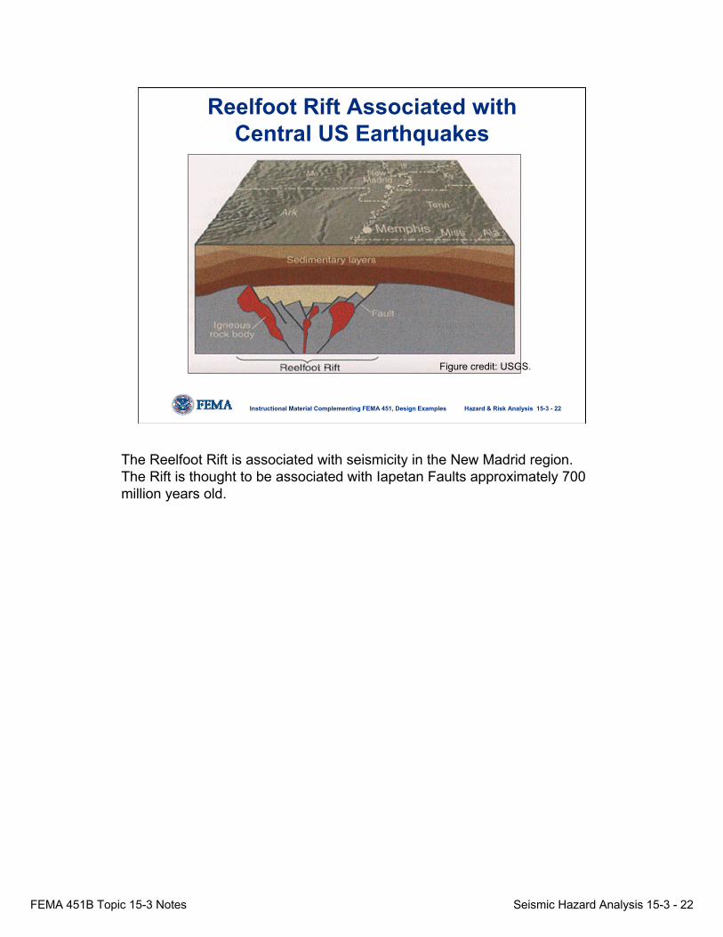
Reelfoot Rift Associated withCentral US Earthquakes
Figure credit: USGS.
The Reelfoot Rift is associated with seismicity in the New Madrid region. The Rift is thought to be associated with Iapetan Faults approximately 700 million years old.
FEMA 451B Topic 15-3 Notes Seismic Hazard Analysis 15-3 - 23
Hazard & Risk Analysis 15-3 - 23Instructional Material Complementing FEMA 451, Design Examples
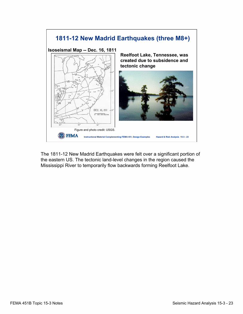
1811-12 New Madrid Earthquakes (three M8+)
Reelfoot Lake, Tennessee, was created due to subsidence and tectonic change
Isoseismal Map -- Dec. 16, 1811
Figure and photo credit: USGS.
The 1811-12 New Madrid Earthquakes were felt over a significant portion of the eastern US. The tectonic land-level changes in the region caused the Mississippi River to temporarily flow backwards forming Reelfoot Lake.
FEMA 451B Topic 15-3 Notes Seismic Hazard Analysis 15-3 - 24
Hazard & Risk Analysis 15-3 - 24Instructional Material Complementing FEMA 451, Design Examples
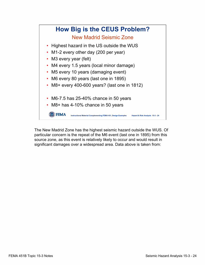
New Madrid Seismic Zone• Highest hazard in the US outside the WUS• M1-2 every other day (200 per year) • M3 every year (felt)• M4 every 1.5 years (local minor damage) • M5 every 10 years (damaging event)• M6 every 80 years (last one in 1895)• M8+ every 400-600 years? (last one in 1812)
• M6-7.5 has 25-40% chance in 50 years• M8+ has 4-10% chance in 50 years
How Big is the CEUS Problem?
The New Madrid Zone has the highest seismic hazard outside the WUS. Of particular concern is the repeat of the M6 event (last one in 1895) from this source zone, as this event is relatively likely to occur and would result in significant damages over a widespread area. Data above is taken from:

FEMA 451B Topic 15-3 Notes Seismic Hazard Analysis 15-3 - 25
Hazard & Risk Analysis 15-3 - 25Instructional Material Complementing FEMA 451, Design Examples
How Big Is the CEUS Problem?• A recurrence of the New Madrid earthquake,
postulated with a 4-10% probability in the next 50 years, has been estimated to cause a total loss potential of $200 billion with 26 states affected.
• Approximately 2/3 of the projected losses will be due to interruptions in business operations and the transport of goods across mid-America.
• This economic loss is of the same order as that caused by the terrorist attacks of September 11, 2001 (NRC, 2003).
The large projected losses associated with to interruptions in business operations and the transport of goods across Mid-America can be better understood when it is considered that many transportation structures, such as key bridges, are very vulnerable to earthquake shaking and typically require long periods before they can be repaired or re-built. Consider the transportation situation in mid-America if key bridges along major highways are down and/or blocking river traffic as well.

FEMA 451B Topic 15-3 Notes Seismic Hazard Analysis 15-3 - 26
Hazard & Risk Analysis 15-3 - 26Instructional Material Complementing FEMA 451, Design Examples
Epicenters of earthquakes (M > 0.0) in the southeastern US from 1977 through 1999.
• Tennessee relatively active
• 1886 South Carolina event not fully explained
• Magnetic signature from North Carolina to Georgia similar to Charleston area; same potential?
Southeastern Seismicity
Figure credit: VTSO
Eastern Tennessee is one of the most active seismic regions in the eastern US. The more small earthquakes occur, the more likely large earthquakes will occur. Thus, the active seismicity in the region is of concern.

FEMA 451B Topic 15-3 Notes Seismic Hazard Analysis 15-3 - 27
Hazard & Risk Analysis 15-3 - 27Instructional Material Complementing FEMA 451, Design Examples
Isoseismal Map from the 1886 Charleston Earthquake
Figure credit: USGS.
Motions for the 1886 Charleston, SC were felt over much of the US reflecting the low rate of attenuation.
FEMA 451B Topic 15-3 Notes Seismic Hazard Analysis 15-3 - 28
Hazard & Risk Analysis 15-3 - 28Instructional Material Complementing FEMA 451, Design Examples
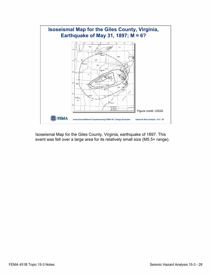
Isoseismal Map for the Giles County, Virginia,Earthquake of May 31, 1897; M ≈ 6?
Figure credit: USGS.
Isoseismal Map for the Giles County, Virginia, earthquake of 1897. This event was felt over a large area for its relatively small size (M5.5+ range).

FEMA 451B Topic 15-3 Notes Seismic Hazard Analysis 15-3 - 29
Hazard & Risk Analysis 15-3 - 29Instructional Material Complementing FEMA 451, Design Examples
Recent Paleoseismological Studies
• Studies in the central and southeastern United States indicate recurring large prehistoric earthquakes – this has increased hazard
• Studies in Pacific Northwest debatable
None.

FEMA 451B Topic 15-3 Notes Seismic Hazard Analysis 15-3 - 30
Hazard & Risk Analysis 15-3 - 30Instructional Material Complementing FEMA 451, Design Examples
Isoseismal Map from the 1886 Charleston Earthquake
Figure credit: USGS.
Motions for the 1886 earthquake in Charleston, South Carolina, were felt over much of the eastern US.
FEMA 451B Topic 15-3 Notes Seismic Hazard Analysis 15-3 - 31
Hazard & Risk Analysis 15-3 - 31Instructional Material Complementing FEMA 451, Design Examples
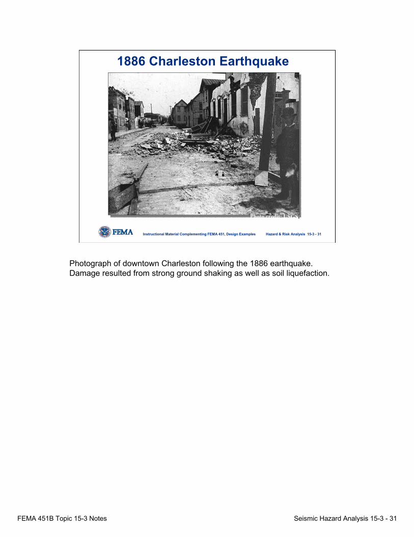
1886 Charleston Earthquake
Photo credit: USGS.
Photograph of downtown Charleston following the 1886 earthquake.Damage resulted from strong ground shaking as well as soil liquefaction.
FEMA 451B Topic 15-3 Notes Seismic Hazard Analysis 15-3 - 32
Hazard & Risk Analysis 15-3 - 32Instructional Material Complementing FEMA 451, Design Examples
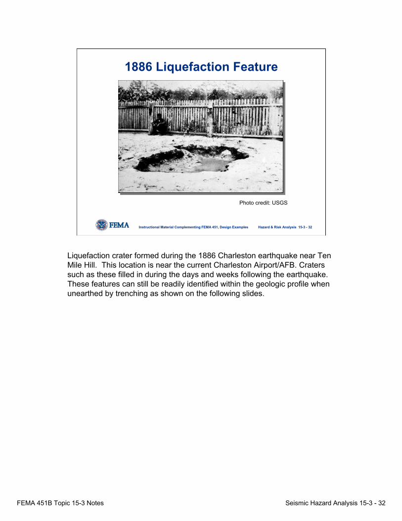
1886 Liquefaction Feature
Photo credit: USGS
Liquefaction crater formed during the 1886 Charleston earthquake near Ten Mile Hill. This location is near the current Charleston Airport/AFB. Craters such as these filled in during the days and weeks following the earthquake. These features can still be readily identified within the geologic profile when unearthed by trenching as shown on the following slides.

FEMA 451B Topic 15-3 Notes Seismic Hazard Analysis 15-3 - 33
Hazard & Risk Analysis 15-3 - 33Instructional Material Complementing FEMA 451, Design Examples
Prehistoric Sand Crater in Trench Wall
Dark material is organic soil and matter
original ground surface
liquefied sands vented from below and eroded crater
outline of crater
~ 1 meter
Photo credit: S. Obermeier
Ancient liquefaction crater found in wall of freshly excavated ditch in the Charleston area. Dark matter is humate-rich soil from the original B-horizon. This material often contains organic material that can be dated using Carbon-14 or other technique. Arrows above delineate the outline of thecrater. Note that the liquefaction occurred in sand beds below the crater and were vented to the ground surface.
FEMA 451B Topic 15-3 Notes Seismic Hazard Analysis 15-3 - 34
Hazard & Risk Analysis 15-3 - 34Instructional Material Complementing FEMA 451, Design Examples
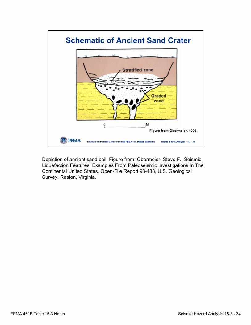
Schematic of Ancient Sand Crater
Figure from Obermeier, 1998.
Depiction of ancient sand boil. Figure from: Obermeier, Steve F., Seismic Liquefaction Features: Examples From Paleoseismic Investigations In The Continental United States, Open-File Report 98-488, U.S. Geological Survey, Reston, Virginia.

FEMA 451B Topic 15-3 Notes Seismic Hazard Analysis 15-3 - 35
Hazard & Risk Analysis 15-3 - 35Instructional Material Complementing FEMA 451, Design Examples
Ages of Earthquake-induced Liquefaction Features Found in Charleston Region*
600 ybp
1250 ybp
3250 ybp
5150 ybp
> 5150 ybp
* Study led to increased seismic design values in South Carolina.
There is still no definitive explanation of the specific causes for these recurrent large (inferred to be) earthquakes in South Carolina. Note: YBP refers to “years before present.” However, the finding of evidence for the repeated occurrence of large earthquakes in that region greatly increased the seismic hazard for that region.

FEMA 451B Topic 15-3 Notes Seismic Hazard Analysis 15-3 - 36
Hazard & Risk Analysis 15-3 - 36Instructional Material Complementing FEMA 451, Design Examples
Virginia Tech Paleoliquefaction Studies
PUGET SOUND REGION
WABASH VALLEY SEISMIC ZONE
CHARLESTON & COASTAL SOUTHCAROLINA
NEW MADRID SEISMIC ZONE
Locations where paleoliquefaction studies have been conducted by researchers from Virginia Tech, USGS, and other agencies and universities.
FEMA 451B Topic 15-3 Notes Seismic Hazard Analysis 15-3 - 37
Hazard & Risk Analysis 15-3 - 37Instructional Material Complementing FEMA 451, Design Examples
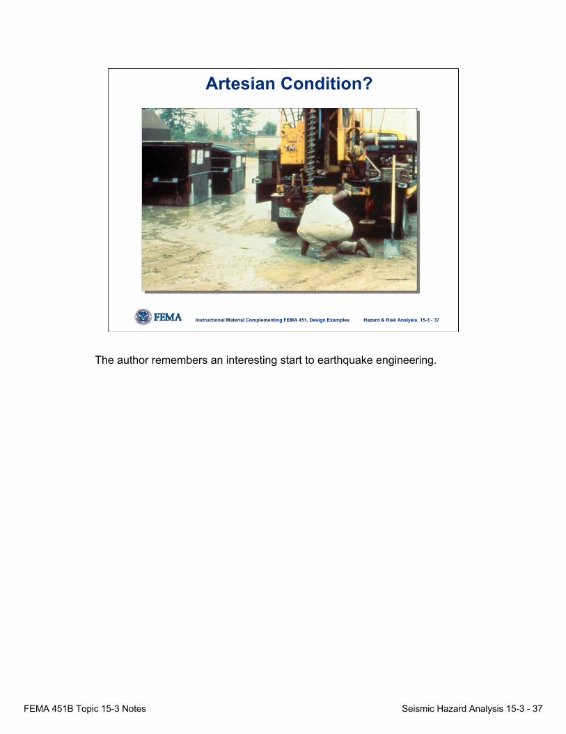
Artesian Condition?
The author remembers an interesting start to earthquake engineering.
FEMA 451B Topic 15-3 Notes Seismic Hazard Analysis 15-3 - 38
Hazard & Risk Analysis 15-3 - 38Instructional Material Complementing FEMA 451, Design Examples
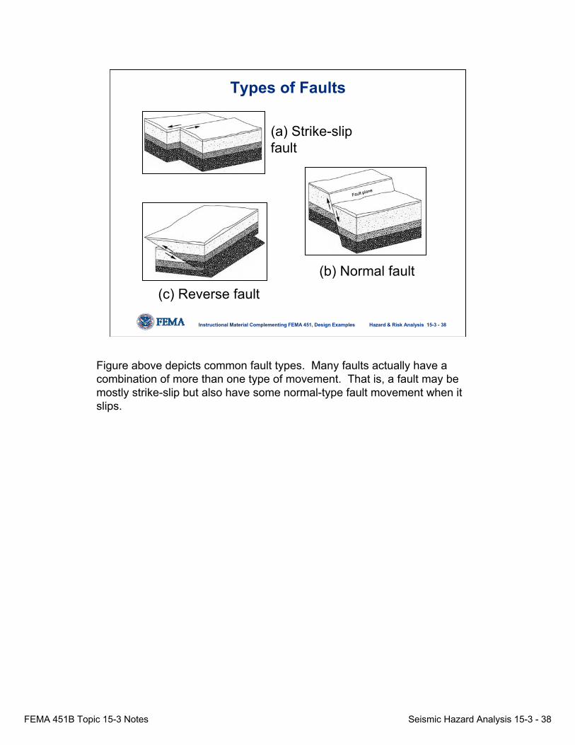
Types of Faults
(c) reverse fault(b) normal fault
(c) Reverse fault(b) Normal fault
(a) Strike-slip fault
Figure above depicts common fault types. Many faults actually have a combination of more than one type of movement. That is, a fault may be mostly strike-slip but also have some normal-type fault movement when it slips.

FEMA 451B Topic 15-3 Notes Seismic Hazard Analysis 15-3 - 39
Hazard & Risk Analysis 15-3 - 39Instructional Material Complementing FEMA 451, Design Examples
New Fence
Time = 0 Years
Fault
Elastic Rebound Theory
What produces seismic waves? The rocks that generate earthquakes have elastic properties that cause them to deform when subjected to tectonic forces (red arrows) and to “snap back” and vibrate when energy is suddenly released. During the rupture, the rough sides of the fault rub against each other. Energy is used up by crushing of rock and by sliding friction. Earthquake waves are generated by both the rubbing and crushing of rock as well as the elastic rebounding of the rocks along adjacent sides of the ruptured fault.

FEMA 451B Topic 15-3 Notes Seismic Hazard Analysis 15-3 - 40
Hazard & Risk Analysis 15-3 - 40Instructional Material Complementing FEMA 451, Design Examples
Old Fence
New Road
Time = 40 Years(strain building)
Fault
The rocks that generate earthquakes have elastic properties and will deform elastically, building up strain energy, in response to the steady tectonic forces (red arrows). The rocks will continue to build up strain energy to a point…

FEMA 451B Topic 15-3 Notes Seismic Hazard Analysis 15-3 - 41
Hazard & Risk Analysis 15-3 - 41Instructional Material Complementing FEMA 451, Design Examples
Old Fence
Time = 41 Years(strain energy released)
New Road
Fault
when the interface resistance along the fault is exceeded, sudden slippage occurs and the rocks “snap back” and vibrate when energy is suddenly released -- we feel the effects of this motion as an earthquake. Earthquake waves are generated by both the rubbing and crushing of rock as well as the elastic rebounding of the rocks along adjacent sides of the ruptured fault. The relative movement along the ruptured portion of the fault results in permanent ground displacement (see offset fence line).

FEMA 451B Topic 15-3 Notes Seismic Hazard Analysis 15-3 - 42
Hazard & Risk Analysis 15-3 - 42Instructional Material Complementing FEMA 451, Design Examples
San Andreas Fault, San Francisco, 1906
Fault trace
Fence offset from fault movement
Photo credit: USGS.
Fence shown above was offset during fault movement associated with the 1906 San Francisco Earthquake with about 3 m of movement.
FEMA 451B Topic 15-3 Notes Seismic Hazard Analysis 15-3 - 43
Hazard & Risk Analysis 15-3 - 43Instructional Material Complementing FEMA 451, Design Examples
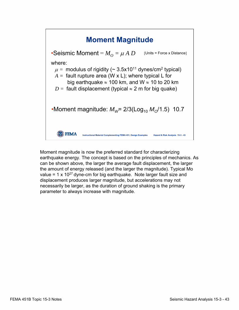
•Seismic Moment = MO = μ A D where:
μ = modulus of rigidity (~ 3.5x10¹¹ dynes/cm2 typical)A = fault rupture area (W x L); where typical L for
big earthquake ≈ 100 km, and W ≈ 10 to 20 kmD = fault displacement (typical ≈ 2 m for big quake)
•Moment magnitude: MW= 2/3(Log10 MO/1.5) 10.7
[Units = Force x Distance]
Moment Magnitude
Moment magnitude is now the preferred standard for characterizing earthquake energy. The concept is based on the principles of mechanics. As can be shown above, the larger the average fault displacement, the larger the amount of energy released (and the larger the magnitude). Typical Mo value = 1 x 1027 dyne-cm for big earthquake. Note larger fault size and displacement produces larger magnitude, but accelerations may not necessarily be larger, as the duration of ground shaking is the primary parameter to always increase with magnitude.

FEMA 451B Topic 15-3 Notes Seismic Hazard Analysis 15-3 - 44
Hazard & Risk Analysis 15-3 - 44Instructional Material Complementing FEMA 451, Design Examples
Earthquake Source and Seismic Waves
• Body waves are generated at the source and they radiate in all directions.• As they go through layers, they are reflected, refracted and transformed.
Fault rupture
P and S waves
Body waves are generated at the source and they radiate in all directions as they go through layers, they are reflected, refracted and transformed. As per Snell’s Law, the wave path is nearly vertical by the time they reach the ground surface.
FEMA 451B Topic 15-3 Notes Seismic Hazard Analysis 15-3 - 45
Hazard & Risk Analysis 15-3 - 45Instructional Material Complementing FEMA 451, Design Examples
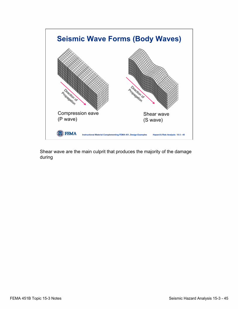
Seismic Wave Forms (Body Waves)
Compression eave(P wave)
Shear wave(S wave)
Direction of
Propagation
Direction of
Propagation
Shear wave are the main culprit that produces the majority of the damage during
FEMA 451B Topic 15-3 Notes Seismic Hazard Analysis 15-3 - 46
Hazard & Risk Analysis 15-3 - 46Instructional Material Complementing FEMA 451, Design Examples
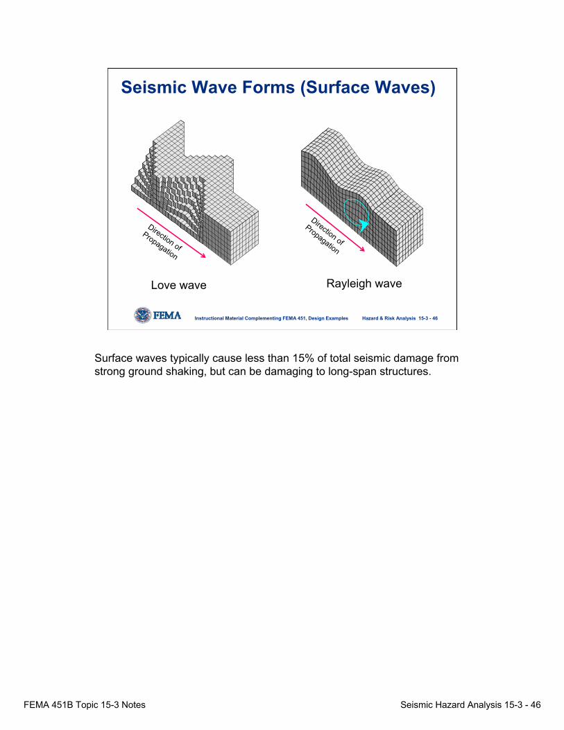
Love wave Rayleigh wave
Seismic Wave Forms (Surface Waves)
Direction of
Propagation
Direction of
Propagation
Surface waves typically cause less than 15% of total seismic damage from strong ground shaking, but can be damaging to long-span structures.

FEMA 451B Topic 15-3 Notes Seismic Hazard Analysis 15-3 - 47
Hazard & Risk Analysis 15-3 - 47Instructional Material Complementing FEMA 451, Design Examples
Earthquake Source and Seismic Waves
P – Primary wavesSH – Horizontally polarized S wavesSV – Vertically polarized S waves
SH PSV
SH
P
SV
Waves bend upwards as they approach the ground surface because of less competent material near the surface – Snell’s Law
Body waves are generated at the source and they radiate in all directions as they go through layers, they are reflected, refracted and transformed. As per Snell’s Law, the wave path is nearly vertical by the time they reach the ground surface.

FEMA 451B Topic 15-3 Notes Seismic Hazard Analysis 15-3 - 48
Hazard & Risk Analysis 15-3 - 48Instructional Material Complementing FEMA 451, Design Examples
Seismic Waves
Direction of wave propagation
Direction of wave propagation
Particle Motions
Vertical Section
Plan View
Rayleigh Love SV PSH
The waves motions of various waves are important, as the horizontally polarized shear wave is our main concern.
FEMA 451B Topic 15-3 Notes Seismic Hazard Analysis 15-3 - 49
Hazard & Risk Analysis 15-3 - 49Instructional Material Complementing FEMA 451, Design Examples
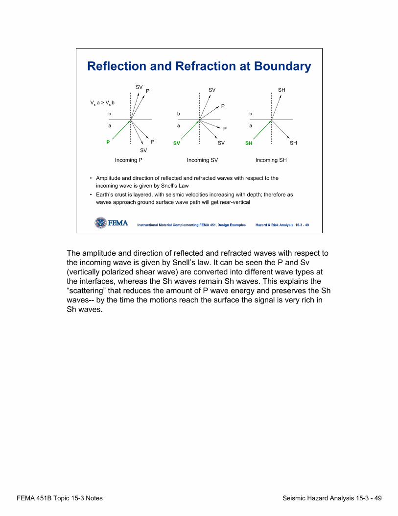
Reflection and Refraction at Boundary
Vs a > Vs b
Incoming P
PSV
P
PSV
a
b
SV
P
SV
P
SV
a
b
SH SH
SH
a
b
Incoming SV Incoming SH
• Amplitude and direction of reflected and refracted waves with respect to the incoming wave is given by Snell’s Law
• Earth’s crust is layered, with seismic velocities increasing with depth; therefore as waves approach ground surface wave path will get near-vertical
The amplitude and direction of reflected and refracted waves with respect to the incoming wave is given by Snell’s law. It can be seen the P and Sv(vertically polarized shear wave) are converted into different wave types at the interfaces, whereas the Sh waves remain Sh waves. This explains the “scattering” that reduces the amount of P wave energy and preserves the Shwaves-- by the time the motions reach the surface the signal is very rich in Sh waves.

FEMA 451B Topic 15-3 Notes Seismic Hazard Analysis 15-3 - 50
Hazard & Risk Analysis 15-3 - 50Instructional Material Complementing FEMA 451, Design Examples
What ground motions at Site A and B? Two steps:1. Define earthquake scenario2. Estimate site response and ground motions
⇒ Must be done in context of structure, type of analysis
Ground Motion Estimation
?Site A
soilrock
fault
Site B
?
Estimating ground motions is made more difficult by the presence of soil deposits which acts as a “filter,” changing the amplitude and frequency of the resultant surface motions from those that occur in hard rock.

FEMA 451B Topic 15-3 Notes Seismic Hazard Analysis 15-3 - 51
Hazard & Risk Analysis 15-3 - 51Instructional Material Complementing FEMA 451, Design Examples
Different Structures, Responses, Analyses, and Issues
The photographs illustrate a series of different structures and site conditions, all of which would respond differently to a given earthquake motion. Therefore the motions used to analyze these structures should be carefully considered – there is no on universal set of ground motions that can be usedto analyze all structures. Remember, the objective is to duplicate the most important characteristics of the potential ground shaking.

FEMA 451B Topic 15-3 Notes Seismic Hazard Analysis 15-3 - 52
Hazard & Risk Analysis 15-3 - 52Instructional Material Complementing FEMA 451, Design Examples
Ground Motion Estimation
• No “universal” set of ground motions for any region.
• Uncertainties are inherent to the process and will cause differences in results.
• Judgment is required, even with probability.
• Inconsistency among governing agencies.
It is important to emphasize that there is no “universal” set of ground motions for any region and that motions to be used will depend upon the specific issue most important to the project (unless of course one can design for all conceivable scenarios, which is economically impossible in most cases).
FEMA 451B Topic 15-3 Notes Seismic Hazard Analysis 15-3 - 53
Hazard & Risk Analysis 15-3 - 53Instructional Material Complementing FEMA 451, Design Examples
Ground Motion Estimation• Two analyses using same models and basic
parameters can give different answers (EPRI vs. NRC/LLNL studies in 1980s).
• Where time and effort are focused during the process is function of structure/system being analyzed.
• Not possible to predict actual motion that will occur at a site; mainly concerned with capturing characteristics important to performance of project.
• Seismologist and engineers must have continuous feedback!
None.

FEMA 451B Topic 15-3 Notes Seismic Hazard Analysis 15-3 - 54
Hazard & Risk Analysis 15-3 - 54Instructional Material Complementing FEMA 451, Design Examples
SPEC
TRA
L A
CC
ELER
ATI
ON
Sa
PERIOD T
SPEC
TRA
L A
CC
ELER
ATI
ON
Sa
PERIOD T
Primary concern for: Primary concern for:
Structure/System Considerations
The short stiff building would be more concerned with the low-period (high-frequency motions) portion of the spectrum, whereas the bridge would be more affected by the energy in the high-period (low frequency motions) portion of the spectrum.

FEMA 451B Topic 15-3 Notes Seismic Hazard Analysis 15-3 - 55
Hazard & Risk Analysis 15-3 - 55Instructional Material Complementing FEMA 451, Design Examples
Structure/System Issues• Place emphasis on issues
important to the specific project.
• Also, think in terms of systemperformance.
Example: If this is not an important part of the spectrum, do not spend extra time and effort on issues that affect this.
Period
SA
It important to place emphasis on the portion of the spectrum that will most affect the structure and its contents.
FEMA 451B Topic 15-3 Notes Seismic Hazard Analysis 15-3 - 56
Hazard & Risk Analysis 15-3 - 56Instructional Material Complementing FEMA 451, Design Examples
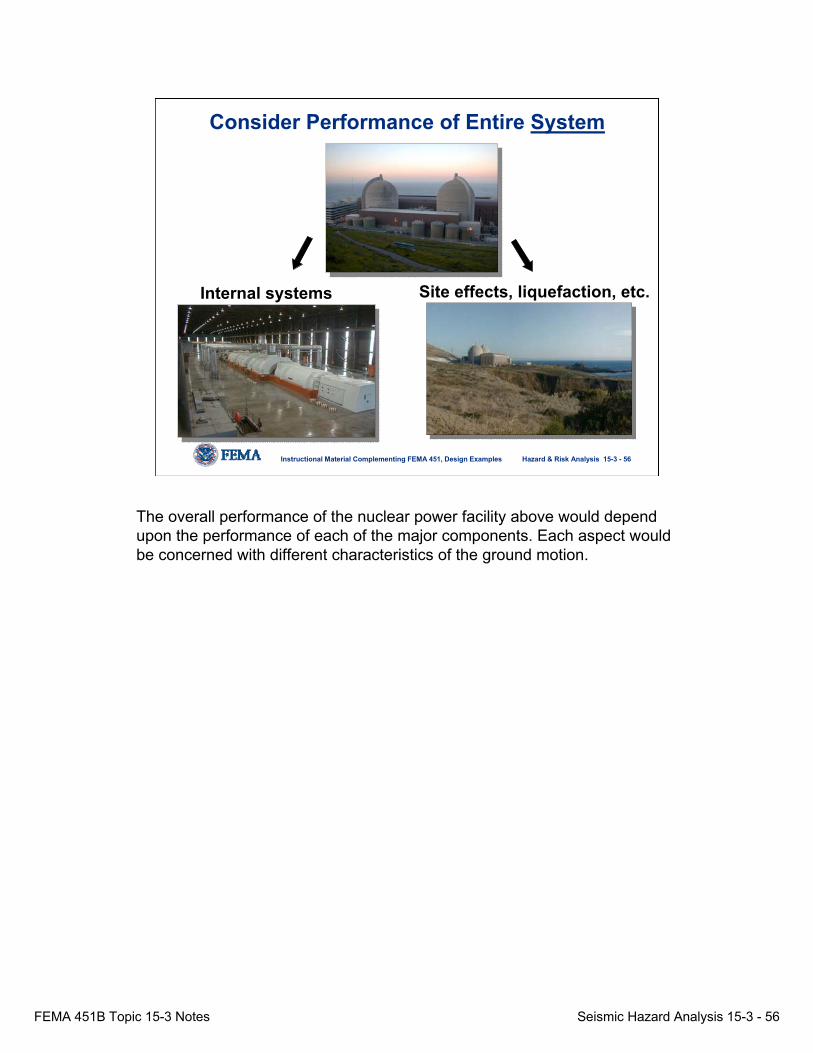
Consider Performance of Entire System
Internal systems Site effects, liquefaction, etc.
The overall performance of the nuclear power facility above would depend upon the performance of each of the major components. Each aspect would be concerned with different characteristics of the ground motion.

FEMA 451B Topic 15-3 Notes Seismic Hazard Analysis 15-3 - 57
Hazard & Risk Analysis 15-3 - 57Instructional Material Complementing FEMA 451, Design Examples
Structure/System Considerations• Type of structure (building, embankment dam, etc.)• Type and purpose of analysis – (linear elastic? time
history? liquefaction?)• Parameters that are important (pga? duration?)• Typical process: seismologist ⇒ geotech engineer ⇒
structural engineer • Seismologists and end user must be closely involved
with continuous feedback• Selection of earthquake scenario is most important
task – (do not want precise analysis of inaccurate model)
None.

FEMA 451B Topic 15-3 Notes Seismic Hazard Analysis 15-3 - 58
Hazard & Risk Analysis 15-3 - 58Instructional Material Complementing FEMA 451, Design Examples
Seismic Hazard and Seismic RiskSeismic hazard evaluation⇒ involves establishing earthquake ground motion parameters for use in evaluating a site/facility during seismic loading. By assessing the vulnerability of the site and the facility under various levels of these ground motion parameters, the seismic risk for the site/facility can then be evaluated.
• Seismic hazard – the expected occurrence of future seismic events• Seismic risk – the expected consequences of future seismic events
None.
FEMA 451B Topic 15-3 Notes Seismic Hazard Analysis 15-3 - 59
Hazard & Risk Analysis 15-3 - 59Instructional Material Complementing FEMA 451, Design Examples
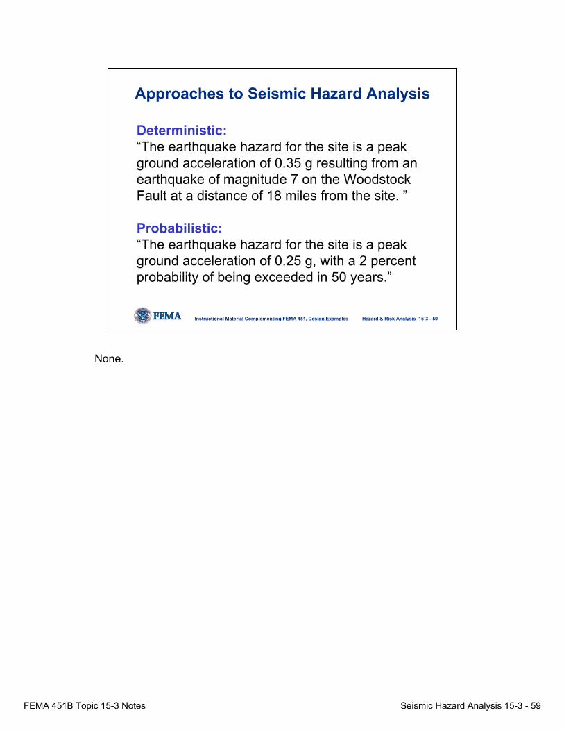
Deterministic:“The earthquake hazard for the site is a peak ground acceleration of 0.35 g resulting from an earthquake of magnitude 7 on the Woodstock Fault at a distance of 18 miles from the site. ”
Probabilistic:“The earthquake hazard for the site is a peak ground acceleration of 0.25 g, with a 2 percent probability of being exceeded in 50 years.”
Approaches to Seismic Hazard Analysis
None.
FEMA 451B Topic 15-3 Notes Seismic Hazard Analysis 15-3 - 60
Hazard & Risk Analysis 15-3 - 60Instructional Material Complementing FEMA 451, Design Examples
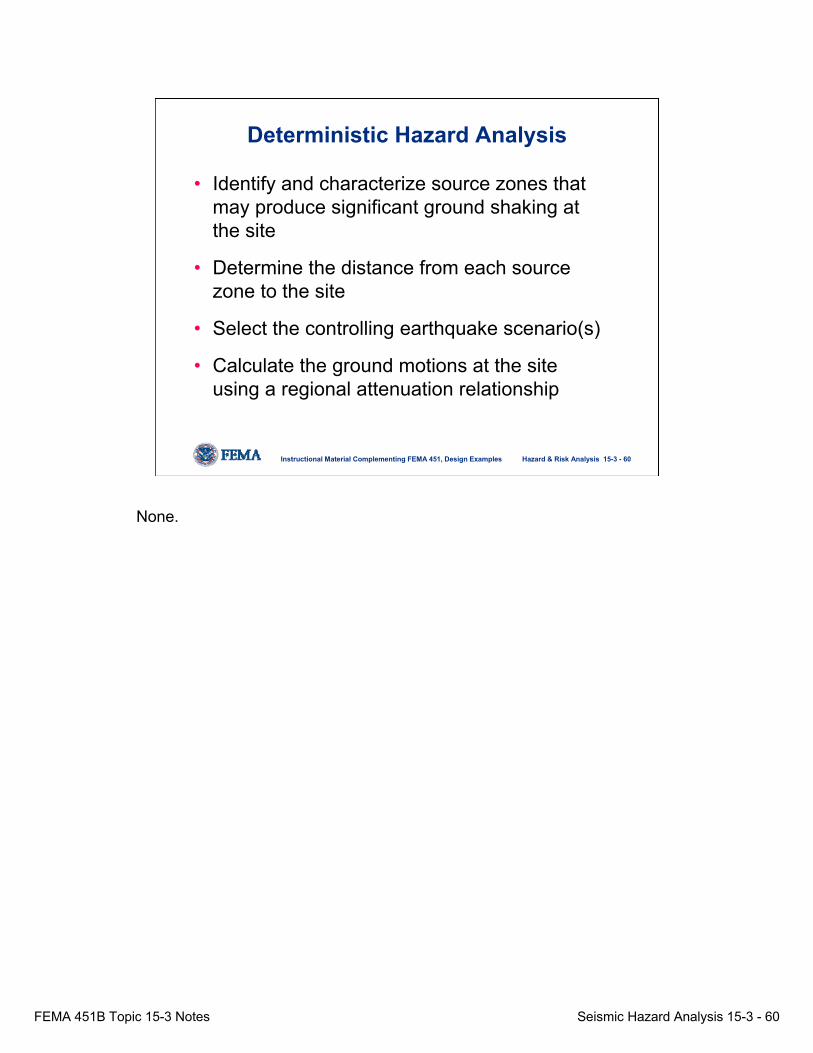
Deterministic Hazard Analysis
• Identify and characterize source zones that may produce significant ground shaking at the site
• Determine the distance from each source zone to the site
• Select the controlling earthquake scenario(s)
• Calculate the ground motions at the site using a regional attenuation relationship
None.
FEMA 451B Topic 15-3 Notes Seismic Hazard Analysis 15-3 - 61
Hazard & Risk Analysis 15-3 - 61Instructional Material Complementing FEMA 451, Design Examples
Ashley River Fault
WoodstockFault
AreaSource
SiteFixed Distance R*
Fixed Magnitude M*
“The earthquake hazard for the site is a pga of 0.35 g resulting from an earthquake of M7 on the Woodstock Fault at a distance of 18 miles from the site. ”
___________*Can use probability to help define these.
Magnitude M
Distance
Pea
k A
ccel
erat
ion
2) Controlling earthquake1) Sources*
4) Hazard at site3) Ground motion attenuation
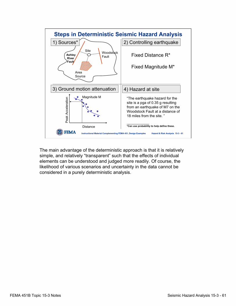
Steps in Deterministic Seismic Hazard Analysis
The main advantage of the deterministic approach is that it is relatively simple, and relatively “transparent” such that the effects of individual elements can be understood and judged more readily. Of course, the likelihood of various scenarios and uncertainty in the data cannot be considered in a purely deterministic analysis.
FEMA 451B Topic 15-3 Notes Seismic Hazard Analysis 15-3 - 62
Hazard & Risk Analysis 15-3 - 62Instructional Material Complementing FEMA 451, Design Examples
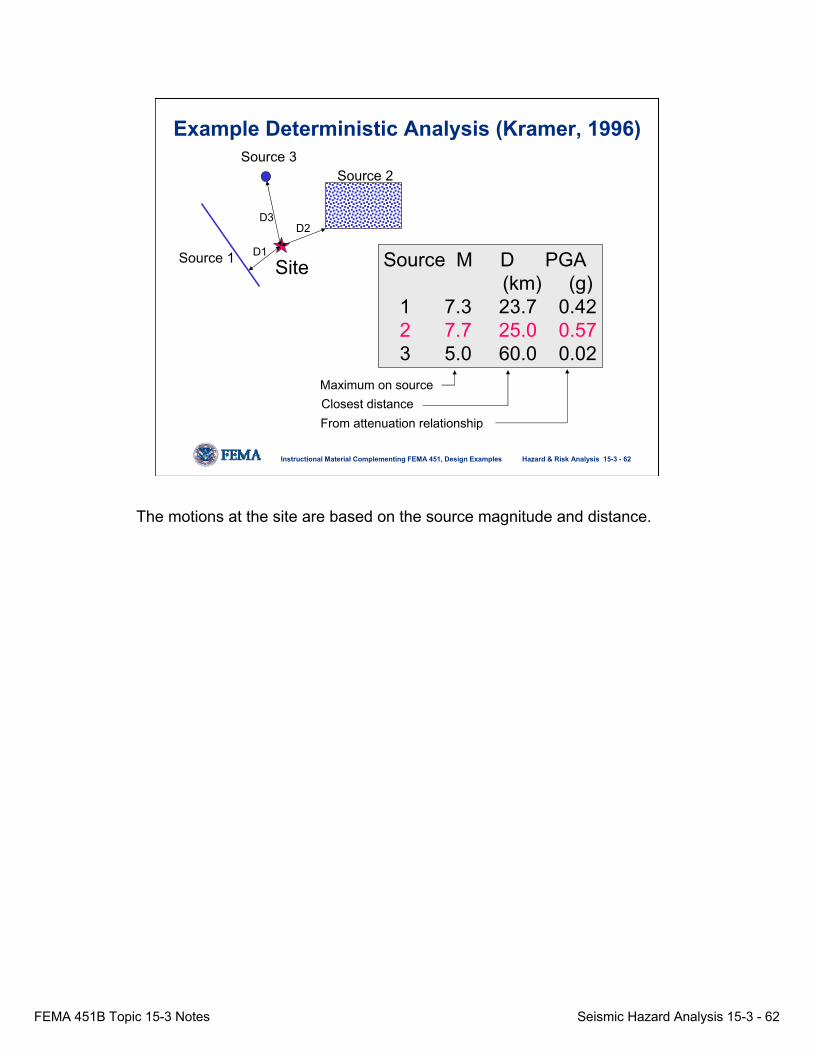
Source 1
Source 2Source 3
Site Source M D PGA(km) (g)
1 7.3 23.7 0.422 7.7 25.0 0.573 5.0 60.0 0.02
D1
D2D3
From attenuation relationshipClosest distanceMaximum on source
Example Deterministic Analysis (Kramer, 1996)
The motions at the site are based on the source magnitude and distance.
FEMA 451B Topic 15-3 Notes Seismic Hazard Analysis 15-3 - 63
Hazard & Risk Analysis 15-3 - 63Instructional Material Complementing FEMA 451, Design Examples
Advantages of Deterministic Approach
• Analysis is relatively “transparent”; effects of individual elements can be understood and judged more readily.
• Requires less expertise than probabilistic analysis.
• Anchored in reality.
Anchored in reality refers to the fact that the scenarios considered by this approach are based on real physical sources (as opposed to some of the results of probabilistic analyses which can correspond to scenarios not physically possible based on fault locations, etc.

FEMA 451B Topic 15-3 Notes Seismic Hazard Analysis 15-3 - 64
Hazard & Risk Analysis 15-3 - 64Instructional Material Complementing FEMA 451, Design Examples
Disadvantages of Deterministic Approach
• Does not consider inherent uncertainties in seismic hazard estimation (i.e., maximum magnitude, ground motion attenuation).
• Relative likelihood of events not considered (EUS vs. WUS); therefore, inconsistent levels of risk.
• Does not allow rational determination of scenario design events in many cases.
• More dependent upon analyst.
None.

FEMA 451B Topic 15-3 Notes Seismic Hazard Analysis 15-3 - 65
Hazard & Risk Analysis 15-3 - 65Instructional Material Complementing FEMA 451, Design Examples
Probabilistic Seismic Hazard Analysis⇒ Considers where, how big, and how often.
• Identify and characterize source zones that may produce significant ground shaking at the site including the spatial distribution and probability of eq’s in each zone.
• Characterize the temporal distribution and probability of earthquakes in each source zone via a recurrence relationship and probability model.
• Select a regional attenuation relationship and associated uncertainty to calculate the variation of ground motion parameters with magnitude & distance.
• Calculate the hazard by integrating over magnitude and distance for each source zone.
Probability basically considers the probability of earthquake of a given magnitude occurring at a given point along a fault multiplied by the probability that the earthquake motions produced by the event will be a certain value at a given location– we thus end up with the probabilistic ground motion for a given site. In the nomenclature of probability theory, the probability of events depends on the probability density distribution that is sampled and the sampling method. For earthquakes, we know neither because we do not understand the physics of earthquake recurrence, so we pick a distribution based on the earthquake history which for most faults is short (only a few recurrences) and complicated. As a result, various distributions consistent with the earthquake history can produce quite different estimates.

FEMA 451B Topic 15-3 Notes Seismic Hazard Analysis 15-3 - 66
Hazard & Risk Analysis 15-3 - 66Instructional Material Complementing FEMA 451, Design Examples
Ashley River Fault
Woodstock Fault
AreaSource
Site
M1
Distance
Pea
k A
ccel
erat
ion
1) Sources
4) Probability of exceedance3) Ground motion
Magnitude M
Log
# Q
uake
s > M
2) Recurrence
M2M3
Considersuncertainty
Pro
babi
lity
of E
xcee
danc
e
Ground Motion Parameter
(Uncertainty in locations of sources & Ms considered).
Steps in Probabilistic Seismic Hazard Analysis
Probability basically considers the probability of earthquake of a given magnitude occurring at a given point along a fault multiplied by the probability that the earthquake motions produced by the event will be a certain value at a given location– we thus end up with the probabilistic ground motion for a given site. A hazard curve tells you what the probability is of any particular strength of ground shaking. It doesn't tell you which value you should choose to design your building against. Do you want to be 95% safe, 99% safe, or 99.9% safe? These are really economic or political decisions, not seismological ones. Also, one has to bear in mind that low probability events do happen. The Maharashtra earthquake of 1993 is a good case in point. If a seismologist had been assessing the hazard in this part of India in 1992, he would have concluded that the probability of a damaging earthquake was extremely low. And he would have been right. Unfortunately, that very small probability came up next year.

FEMA 451B Topic 15-3 Notes Seismic Hazard Analysis 15-3 - 67
Hazard & Risk Analysis 15-3 - 67Instructional Material Complementing FEMA 451, Design Examples
0.0001
0.001
0.01
0.1
1
10
100
1000
0 2 4 6 8 10
Magnitude
Mea
n A
nnua
l Rat
e of
Exc
eeda
nce
bmam −=λlog
mλ = mean rate ofrecurrence(events/year)
a and b to be deter-mined from data; bis typically about 1.0
λ m
mλ/1 = return period
Empirical Gutenberg-RichterRecurrence Relationship
The number of earthquake of a given magnitude, based on seismic network monitoring, are used to determine recurrence relationships and/or or the rate of earthquake of various magnitudes. The number of small earthquakes is much greater than the number of large earthquakes. The number of frequent small events is used to estimate the probable rate of large events.

FEMA 451B Topic 15-3 Notes Seismic Hazard Analysis 15-3 - 68
Hazard & Risk Analysis 15-3 - 68Instructional Material Complementing FEMA 451, Design Examples
Attenuation Laws Recurrence Relationship
Distance to Site
][][],*[1 1 1
* kjkj
N
i
N
j
N
kiy rRPmMPrmyYPv
S M R
==>= ∑∑∑= = =
λ
Uncertainties Included inProbabilistic Analysis
We do not really know with confidence many of the input parameters required for seismic hazard analysis in CEUS. The above equation is complicated, but the equation simply result in the determination of one
parameter– the mean annual rate of earthquakes, λ. This is used in the Poisson model to estimate the probability of earthquakes shaking exceeding a certain value. Note that a ground shaking level (i.e., PGA) is assumed and the probability of exceeding this value is computed. Thus, the ground motion is actually the independent variable, while the probability is the dependent variable. After many probability-ground motions pairs are determined, the results are typically plotted in map form with contours of ground motions for a given probability of exceedance; see current USGS maps. On a given seismic hazard map for a given probability of exceedance (PE), locations shaken more frequently will have larger ground motions. Plotted in this manner, the maps suggest that the ground motion is the dependent variable; however, the probability is actually the dependent variable. Note the rate parameter above is used in the Poisson model in several of the following slides.
FEMA 451B Topic 15-3 Notes Seismic Hazard Analysis 15-3 - 69
Hazard & Risk Analysis 15-3 - 69Instructional Material Complementing FEMA 451, Design Examples
We Commonly Use Two Approaches to Predict the Likelihood of Earthquakes
• Time-independent (Poisson Model)
• Time-dependent Models
The difference is that for times since the previous earthquake less than about 2/3 of the assumed recurrence interval, the Poisson model predicts higher probabilities. At later times a Gaussian model predicts progressively greater probabilities. For example, consider estimating the probability of a major New Madrid earthquake in the next 20 years, assuming that the past one occurred in 1812. If we assume these earthquakes have a meanrecurrence of 500 years with standard deviation 100 years, the time dependant (Gaussian) probability is 0.1%, whereas the time independent probability is 4%. If instead we assume mean recurrence of 750 years and standard deviation 100 years, the probabilities are 0.3% and 3%. Weibulland log-normal distributions would give other values. Hence the probability we estimate depends on the distribution we chose and the numerical parameters we chose for that distribution. We pick what we want, and get the answer we wish. The tendency in the Midwest has been to use Poisson models, which give higher earthquake probabilities than the time-dependant models because we're still close to 1812. Conversely in California, most applications use time-dependant models. Even with good paleoseismic data, one gets quite a range of probability estimates. For example at Pallet Creek on the San Andreas the most recent five major earthquakes yield recurrence with a mean and standard deviation of 194 and 58 years, whereas the past ten earthquakes yield 132 and 105. Thus in 1989 the range of probabilities for a major earthquake before 2019 was estimated as about 7-51%. If this is what 10 earthquake cycles give, the implications for New Madrid where we have only 3 or 4 are obvious.
FEMA 451B Topic 15-3 Notes Seismic Hazard Analysis 15-3 - 70
Hazard & Risk Analysis 15-3 - 70Instructional Material Complementing FEMA 451, Design Examples
Poisson Model
• The simplest, most used model for earthquake probability.
• It is a time-independent model -- the probability that an earthquake will occur in an interval of time starting from now does not depend on when "now" is, because a Poisson process has no "memory."
The simplest model for earthquake occurrence is a time-independent Poisson model, in which the probability that an earthquake will occur in an interval of time starting from now does not depend on when "now" is, because a Poisson process has no "memory".

FEMA 451B Topic 15-3 Notes Seismic Hazard Analysis 15-3 - 71
Hazard & Risk Analysis 15-3 - 71Instructional Material Complementing FEMA 451, Design Examples
Poisson Distribution (general form)
P (X = k) = (λt)k e-(λt)
k!
where λ = rate (events/year)t = exposure intervalk = no. of events
The simplest model for earthquake occurrence is a time-independent Poisson model, in which the probability that an earthquake will occur in an interval of time starting from now does not depend on when "now" is, because a Poisson process has no "memory". This method is used in probabilistic analysis of both earthquake, floods, and other natural disasters.
FEMA 451B Topic 15-3 Notes Seismic Hazard Analysis 15-3 - 72
Hazard & Risk Analysis 15-3 - 72Instructional Material Complementing FEMA 451, Design Examples
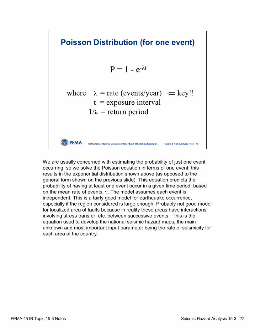
Poisson Distribution (for one event)
P = 1 - e-λt
where λ = rate (events/year) ⇐ key!!t = exposure interval
1/λ = return period
We are usually concerned with estimating the probability of just one event occurring, so we solve the Poisson equation in terms of one event; this results in the exponential distribution shown above (as opposed to the general form shown on the previous slide). This equation predicts the probability of having at least one event occur in a given time period, based on the mean rate of events, ν. The model assumes each event is independent. This is a fairly good model for earthquake occurrence, especially if the region considered is large enough. Probably not good model for localized area of faults because in reality these areas have interactions involving stress transfer, etc. between successive events. This is the equation used to develop the national seismic hazard maps, the main unknown and most important input parameter being the rate of seismicity for each area of the country.

FEMA 451B Topic 15-3 Notes Seismic Hazard Analysis 15-3 - 73
Hazard & Risk Analysis 15-3 - 73Instructional Material Complementing FEMA 451, Design Examples
Poisson Model• Note that the probabilistic earthquake risk level can
be put in the form of an earthquake return interval:
Earthquake Return Period = t/-ln(1-PE)
ReturnPE t Period10% 50 yrs. 4755% 50 yrs. 9752% 50 yrs. 2475
Note that when the exponent of the equation, λt, is small, then P ≈ λt.
Note that for low probabilities (or long return periods), the return period is approximately t/PE such that T is about = 50/0.02 = 2,500 years. This approximation works fine for low probabilities or long return periods, but does not work well for higher probabilities. For instance, the actual return period of 50% PE in 50 Years is 72 years, not 100 years as suggested by the approximate formula.
FEMA 451B Topic 15-3 Notes Seismic Hazard Analysis 15-3 - 74
Hazard & Risk Analysis 15-3 - 74Instructional Material Complementing FEMA 451, Design Examples
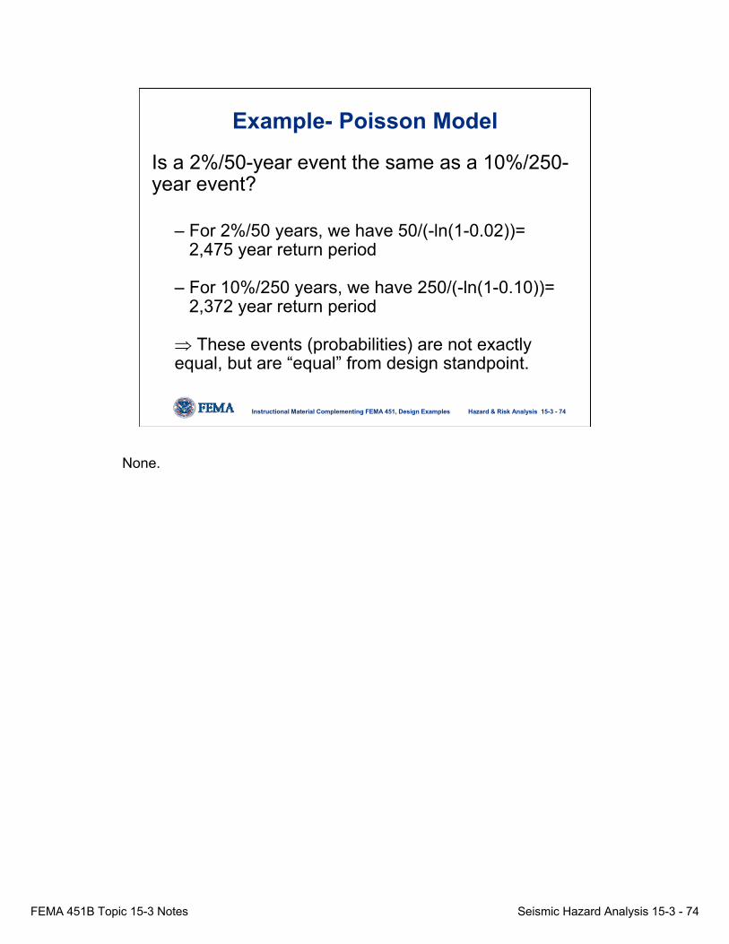
Example- Poisson Model
Is a 2%/50-year event the same as a 10%/250-year event?
– For 2%/50 years, we have 50/(-ln(1-0.02))=2,475 year return period
– For 10%/250 years, we have 250/(-ln(1-0.10))= 2,372 year return period
⇒ These events (probabilities) are not exactly equal, but are “equal” from design standpoint.
None.

FEMA 451B Topic 15-3 Notes Seismic Hazard Analysis 15-3 - 75
Hazard & Risk Analysis 15-3 - 75Instructional Material Complementing FEMA 451, Design Examples
Time-Dependent Models• Used less than simpler Poisson model• Time-dependent means that the probability of
a large earthquake is small immediately after the last, and then grows with time.
• Such models use various probability density functions to describe the time between earthquakes including Gaussian, log-normal, and Weibull distributions.
Alternative models are time-dependant, in which the probability of a large earthquake is small immediately after the last, and then grows with time. Such models use various probability density functions to describe the time between earthquakes. These include Gaussian, log- normal, and Weibull distributions, each of which give different numbers. Again, as mentioned in the previous slide, the difference is that for times since the previous earthquake less than about 2/3 of the assumed recurrence interval, the Poisson model predicts higher probabilities. At later times a Gaussian model predicts progressively greater probabilities. For example, consider estimating the probability of a major New Madrid earthquake in the next 20 years, assuming that the past one occurred in 1812. If we assume these earthquakes have a mean recurrence of 500 years with standard deviation 100 years, the time dependant (Gaussian) probability is 0.1%, whereas the time independent probability is 4%. If instead we assume mean recurrence of 750 years and standard deviation 100 years, the probabilities are 0.3% and 3%. Weibull and log-normal distributions would give other values. Hence the probability we estimate depends on the distribution we chose and the numerical parameters we chose for that distribution. We pick what we want, and get the answer we wish. The tendency in the Midwest has been to use Poisson models, which give higher earthquake probabilities than the time-dependant models because we're still close to 1812. Conversely in California, most applications use time-dependant models. Even with good paleoseismic data, one gets quite a range of probability estimates. For example at Pallet Creek on the San Andreas the most recent five major earthquakes yield recurrence with a mean and standard deviation of 194 and 58 years, whereas the past ten earthquakes yield 132 and 105. Thus in 1989 the range of probabilities for a major earthquake before 2019 was estimated as about 7-51%. If this is what 10 earthquake cycles give, the implications for New Madrid where we have only 3 or 4 are obvious.

FEMA 451B Topic 15-3 Notes Seismic Hazard Analysis 15-3 - 76
Hazard & Risk Analysis 15-3 - 76Instructional Material Complementing FEMA 451, Design Examples
Source 1
Source 2Source 3
Site
D1=?D2=?D3
Source 1
Source 2
Source 3
SiteM2=?
M3=?
M1=?A1=?
A3=?
A2=?
Example Probabilistic Analysis (Kramer)
The PSHA analyses consider all magnitudes (large enough to causedamage, typically M5 and above) from all sources at all distances. The sources vary from specific faults to large area sources (box in figure above) or in many case, a background source (the entire region in which it is determined that earthquake could occur anywhere in the general region–such as the Piedmont region of the south east).
FEMA 451B Topic 15-3 Notes Seismic Hazard Analysis 15-3 - 77
Hazard & Risk Analysis 15-3 - 77Instructional Material Complementing FEMA 451, Design Examples
Source 1
Source 2Source 3
Site
0.0 0.2 0.4 0.6 0.8
10-6
10-4
10-2
10-0
10-7
10-5
10-3
10-1
10-1
10-8
Peak Horizontal Acceleration (g)Mea
n An
nual
Rat
e of
Exc
eeda
nce
Source 1
Source 2
Source 3
All Source Zones
SEISMIC HAZARD CURVE
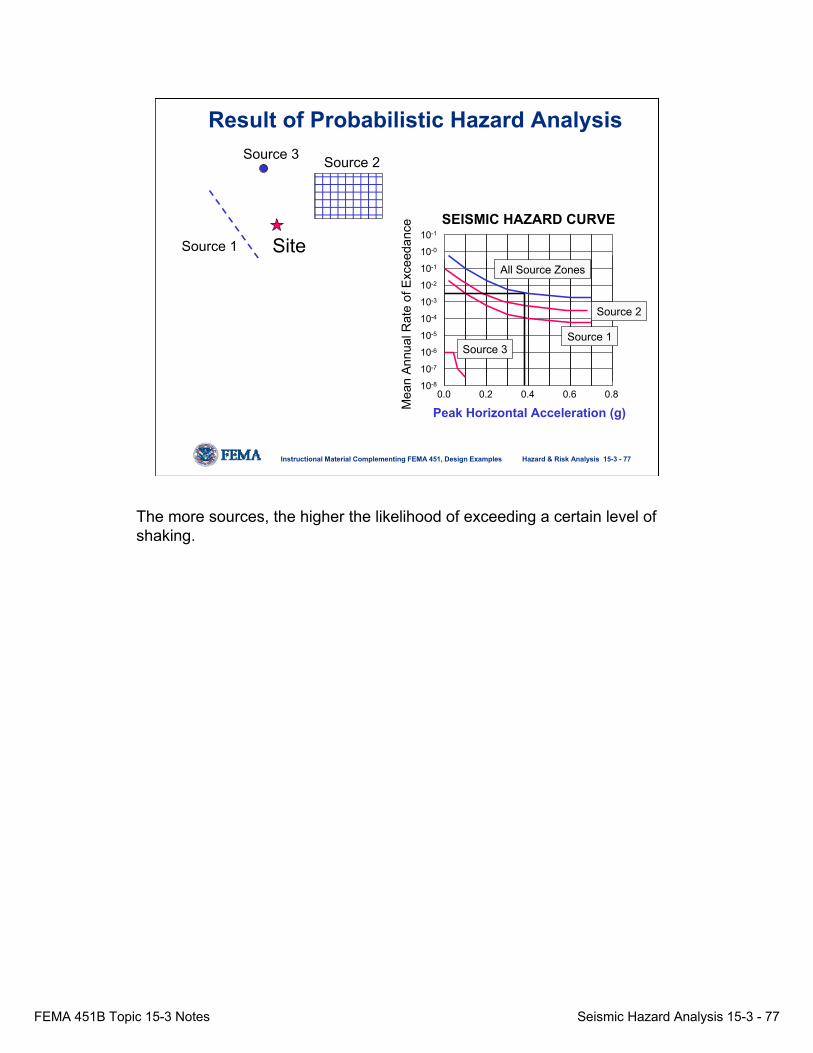
Result of Probabilistic Hazard Analysis
The more sources, the higher the likelihood of exceeding a certain level of shaking.
FEMA 451B Topic 15-3 Notes Seismic Hazard Analysis 15-3 - 78
Hazard & Risk Analysis 15-3 - 78Instructional Material Complementing FEMA 451, Design Examples
0.0 0.2 0.4 0.6 0.8
10-6
10-4
10-2
10-0
10-7
10-5
10-3
10-1
10-1
10-8
Peak Horizontal Acceleration (g)
Mea
n An
nual
Rat
e of
Exc
eeda
nce SEISMIC HAZARD CURVE
PGA = 0.33g
10% Probability in 50 yearsReturn Period = 475 yearsRate of Exceedance = 1/475=0.0021
Period, T (sec)
Acc
eler
atio
n, g
0.0 0.5 1.0 1.5
0.2
0.4
0.6
0.810% in 50 YearElastic ResponseSpectrum
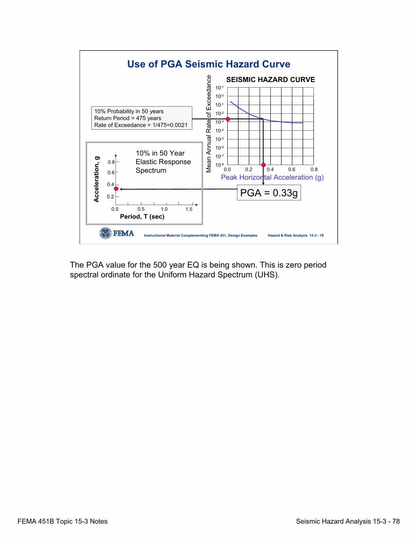
Use of PGA Seismic Hazard Curve
The PGA value for the 500 year EQ is being shown. This is zero period spectral ordinate for the Uniform Hazard Spectrum (UHS).

FEMA 451B Topic 15-3 Notes Seismic Hazard Analysis 15-3 - 79
Hazard & Risk Analysis 15-3 - 79Instructional Material Complementing FEMA 451, Design Examples
0.0 0.2 0.4 0.6 0.8
10-6
10-4
10-2
10-0
10-7
10-5
10-3
10-1
10-1
10-8
0.2 Sec Spectral Acceleration (g)
Mea
n An
nual
Rat
e of
Exc
eeda
nce SEISMIC HAZARD CURVE
0.2 Sec accn = 0.55g
10% Probability in 50 yearsReturn Period = 475 yearsRate of Exceedance = 1/475=0.0021
Period, T (sec)
Acc
eler
atio
n, g
0.0 0.5 1.0 1.5
0.2
0.4
0.6
0.8
10% in 50 yearElastic ResponseSpectrum
Use of 0.2 Sec. Seismic Hazard Curve
The 0.2 second spectral ordinate for the 500 year EQ is being shown. This is o.2 secpond spectral ordinate for the Uniform Hazard Spectrum (UHS).

FEMA 451B Topic 15-3 Notes Seismic Hazard Analysis 15-3 - 80
Hazard & Risk Analysis 15-3 - 80Instructional Material Complementing FEMA 451, Design Examples
Period, T (sec)
Acc
eler
atio
n, g
0.0 0.5 1.0 1.5
0.2
0.4
0.6
0.8
10% in 50 year ElasticResponse Spectrum (UHS)
10% in 50 year elastic response spectrum developed from the curves shown in the previous slides and additional points.

FEMA 451B Topic 15-3 Notes Seismic Hazard Analysis 15-3 - 81
Hazard & Risk Analysis 15-3 - 81Instructional Material Complementing FEMA 451, Design Examples
Large DistantEarthquake
Small NearbyEarthquake
Uniform Hazard Spectrum
Period
Response
Uniform Hazard Spectrum (UHS)
Using the UHS as a basis for spectrum matching to establish a single earthquake motion is incorrect; the extent of the issues associated with this procedures depends upon the depends upon the specifics of the analysis, such as the region of the country. That is, in northern California where the seismicity in San Francisco is dominated by the nearby San Andreas fault, the UHS and the deterministic spectra will probably be very similar because the hazard is so dominated by a single event.

FEMA 451B Topic 15-3 Notes Seismic Hazard Analysis 15-3 - 82
Hazard & Risk Analysis 15-3 - 82Instructional Material Complementing FEMA 451, Design Examples
• Developed from probabilistic analysis.
• Represents contributions from small local and large distant earthquakes.
• May be overly conservative for modal response spectrum analysis.
• May not be appropriate for artificial ground motion generation, especially in CEUS.
Uniform Hazard Spectrum
None.
FEMA 451B Topic 15-3 Notes Seismic Hazard Analysis 15-3 - 83
Hazard & Risk Analysis 15-3 - 83Instructional Material Complementing FEMA 451, Design Examples
Advantages of Probabilistic Approach• Reflects true state of knowledge and lack
thereof.• Consider inherent uncertainties in seismic
hazard estimation (i.e., maximum magnitude, ground motion attenuation).
• Considers likelihood of events considered; basis for consistent levels of risk established.
• Allows more rationale comparison among many scenarios and to other hazards.
• Less dependent upon analyst.
None.
FEMA 451B Topic 15-3 Notes Seismic Hazard Analysis 15-3 - 84
Hazard & Risk Analysis 15-3 - 84Instructional Material Complementing FEMA 451, Design Examples
Disadvantages of Probabilistic Approach• Analyses are not transparent; the effects of individual
parameters cannot be easily recognized and understood.
• “Quantitatively seductive” -- encourages use of precision that is out of proportion with the accuracy with which the input is known.
• Requires special expertise.
• May provide unrealistic scenarios (i.e., probabilistic design event could correspond to location where actual fault does not exist).
• Analyst still has big influence (methods, etc.).
Since the probabilities we estimate depend on many choices, it may no be wise to focus on specific numbers. It may make more sense to quote probabilities in broad ranges, such as low (<10%), intermediate (10-90%), or high (>90%).

FEMA 451B Topic 15-3 Notes Seismic Hazard Analysis 15-3 - 85
Hazard & Risk Analysis 15-3 - 85Instructional Material Complementing FEMA 451, Design Examples
Probabilistic vs. Deterministic
• Results of probabilistic and deterministic analyses are often similar in the WUS; not true for CEUS.
• Deterministic scenarios typically very difficult to define in CEUS.
• Best to use integrated or hybrid method that combines both approaches.
Both approaches can be combined to take advantage of the best attributes of both. This approach is used in the example project in central IL and IN shown in the following slides.

FEMA 451B Topic 15-3 Notes Seismic Hazard Analysis 15-3 - 86
Hazard & Risk Analysis 15-3 - 86Instructional Material Complementing FEMA 451, Design Examples
Deaggregation of the PSHA• Each bar represents an event that exceeds a specifiedground motion at 1 Hz – Washington, DC, example.; note mean and modal values.
The deaggregation plot above indicates the relative contribution of different earthquakes of different sizes at different distances in the Washington, DC area. The values reflect the relative contribution toward the spectral acceleration value of the UHS at 1 Hz. It is important to understand the significance between the mean and the modal events, as the modal event is the most likely event and the mean reflects the average scenario.

FEMA 451B Topic 15-3 Notes Seismic Hazard Analysis 15-3 - 87
Hazard & Risk Analysis 15-3 - 87Instructional Material Complementing FEMA 451, Design Examples
Hazard Scenario – Example
Project SiteProject Site
ILLINOISILLINOIS
The figure above illustrates two different sources zones that can affect the project site. Each of the source zones contain multiple faults that can generate earthquakes of different sizes. For a site such as that above where there are many different sources at different distances and of different magnitudes, probability is best tool to use to determine which earthquake scenarios are most critical to design for. The primary end objective was to develop an appropriate set of acceleration time histories for the design of the facility.
FEMA 451B Topic 15-3 Notes Seismic Hazard Analysis 15-3 - 88
Hazard & Risk Analysis 15-3 - 88Instructional Material Complementing FEMA 451, Design Examples
Period (sec)0.1 1
PS
A (m
/s2 )
0
1
2
3
4
5
6
For 5% damping
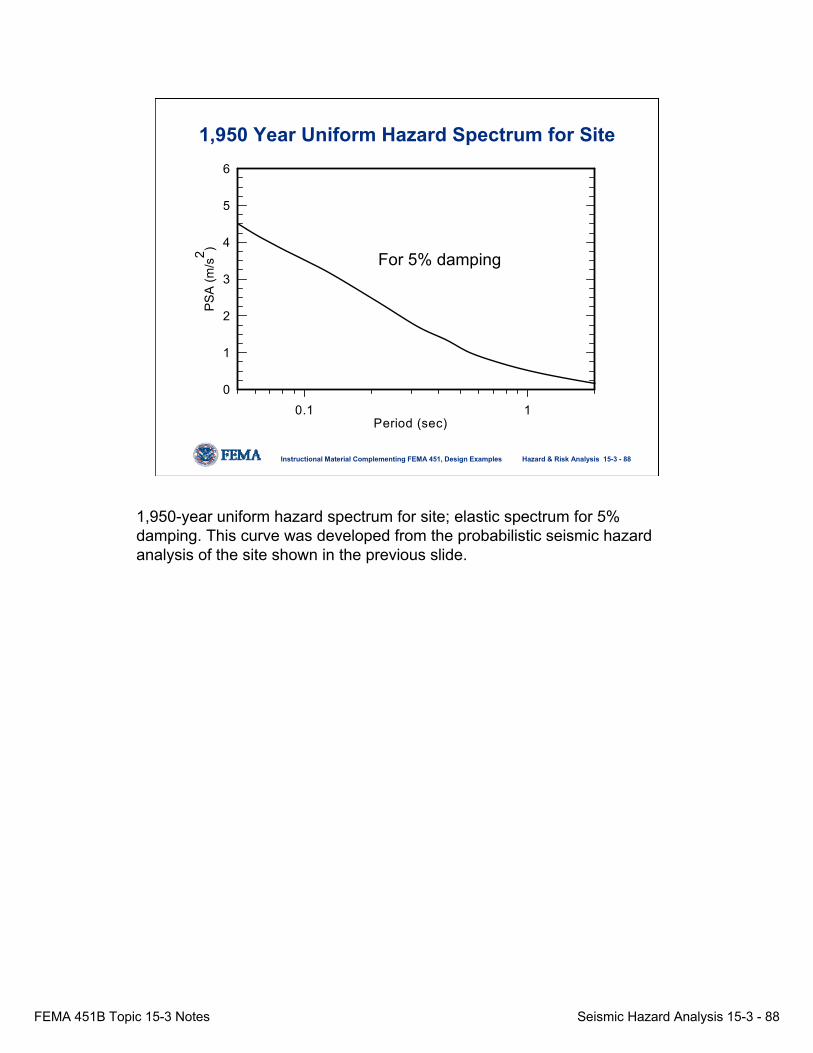
1,950 Year Uniform Hazard Spectrum for Site
1,950-year uniform hazard spectrum for site; elastic spectrum for 5% damping. This curve was developed from the probabilistic seismic hazard analysis of the site shown in the previous slide.
FEMA 451B Topic 15-3 Notes Seismic Hazard Analysis 15-3 - 89
Hazard & Risk Analysis 15-3 - 89Instructional Material Complementing FEMA 451, Design Examples
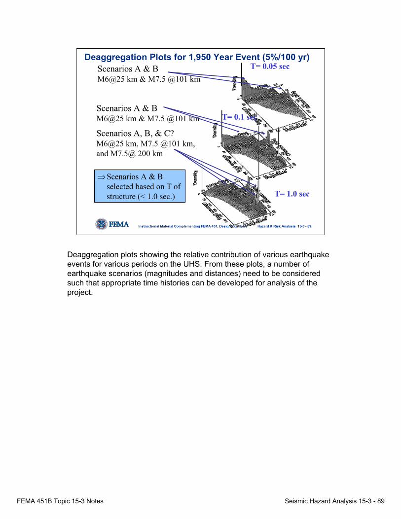
Deaggregation Plots for 1,950 Year Event (5%/100 yr)T= 0.05 sec
T= 0.1 sec
T= 1.0 sec
Scenarios A & BM6@25 km & M7.5 @101 km
Scenarios A & BM6@25 km & M7.5 @101 km
Scenarios A, B, & C?M6@25 km, M7.5 @101 km, and M7.5@ 200 km
⇒ Scenarios A & B selected based on T of structure (< 1.0 sec.)
Deaggregation plots showing the relative contribution of various earthquake events for various periods on the UHS. From these plots, a number of earthquake scenarios (magnitudes and distances) need to be considered such that appropriate time histories can be developed for analysis of the project.

FEMA 451B Topic 15-3 Notes Seismic Hazard Analysis 15-3 - 90
Hazard & Risk Analysis 15-3 - 90Instructional Material Complementing FEMA 451, Design Examples
From the top, vertical, North-South and East-West components
Stochastic Simulations of Ground Acceleration for M = 6.0 at 25 km (Scenario A)
Stochastic simulations of ground acceleration for M = 6.0 at 25 km (Scenario A); this was one of the two scenarios considered for the design of the facility.

FEMA 451B Topic 15-3 Notes Seismic Hazard Analysis 15-3 - 91
Hazard & Risk Analysis 15-3 - 91Instructional Material Complementing FEMA 451, Design Examples
Vertical, fault normal and fault parallel refer to finite fault calculations, and show 3-orthogonal components of motion, oriented with respect to source
Stochastic Simulations of Ground Acceleration forM = 7.5 at 101 km (Scenario B)
Stochastic simulations of ground acceleration for M = 7.5 at 101 km (Scenario B); this was one of the two scenarios considered for the design of the facility.
FEMA 451B Topic 15-3 Notes Seismic Hazard Analysis 15-3 - 92
Hazard & Risk Analysis 15-3 - 92Instructional Material Complementing FEMA 451, Design Examples
Discussion of Selected Scenarios A & B
• What kind of analysis to be performed?
• Is duration important, or just pga?
• Basic question: “Does it matter which event caused motions to be exceeded?”
• Seismologist and end user should be closely linked from the beginning!!
It is possible to perform analyses for all possible sources and distances, but often there is too little budget. It must be determined which scenario is the most critical. Which event is most critical depends upon many issues, such as whether duration as well as PGA is important (most geotechnical analyses), or whether PGA is the main consideration (most structural analyses).

FEMA 451B Topic 15-3 Notes Seismic Hazard Analysis 15-3 - 93
Hazard & Risk Analysis 15-3 - 93Instructional Material Complementing FEMA 451, Design Examples
National Seismic Hazard Maps • Developed by U.S. Geological Survey.
• Adopted (almost exactly) by building codes and reference standards (i.e., IBC2003) and, therefore, very important!!!
• Based on probability ⇒ maps show contours of maximum expected ground motion for a given level of certainty (90%, 98%, etc.) in 50 years; or, said differently, contours of ground motions that have a common given probability of exceedance, PE, in 50 years (10%, 2%, etc.).
The specific basis for originally selecting these three specific probability levels for mapping and use in engineering design is somewhat moot and is probably a remnant of the first series of seismic safety analyses performed for nuclear power facilities in the late 1960s and 1970s when probabilistic seismic hazard analysis techniques were being originally developed. These probabilities have become the “standard” probability levels frequently referred to and used in seismic design. The 2%/50-year map is used as the basis for structural design in most regions

FEMA 451B Topic 15-3 Notes Seismic Hazard Analysis 15-3 - 94
Hazard & Risk Analysis 15-3 - 94Instructional Material Complementing FEMA 451, Design Examples
Earthquake Probability Levels• Note that the term “2500 year earthquake”
does not indicate an event that occurs once every 2,500 years!
• Rather, this term reflects a probability, that is, the earthquake event that has a probability of 1 in 2500 of occurring in one year.
• For instance, the “100-year flood” can actually occur several years in a row or even several times in one year (as occurred in the 1990s in Virginia).
This term is commonly misunderstood and misinterpreted. The term “2500 year earthquake” does not indicate that an event that occurs once every 2,500 years! Rather, this term reflects a probability, that is, the earthquake event that has a probability of 1 in 2500 of occurring in one year. For instance, the “100-year flood” can actually occur several years in a row or even several times in one year (as occurred in the 1990s in Virginia). The Poisson model is used to predict the probability of earthquakes based on the average rate of earthquakes of a given size that occur in a region—hence the importance of seismic monitoring networks that record earthquakes, including the frequent small events that are not felt. A statically representative data catalog of the number of earthquakes of various size forms the basis for estimating the likelihood of future events, including large damaging earthquakes. The more data available, the better the predictions (at least statistically). For more on the discussion of probability associated with the maps, see FAQs at: http://geohazards.cr.usgs.gov/eq/html/faq.htmland/or: “Info for the Layman” at http://geohazards.cr.usgs.gov/eq/

FEMA 451B Topic 15-3 Notes Seismic Hazard Analysis 15-3 - 95
Hazard & Risk Analysis 15-3 - 95Instructional Material Complementing FEMA 451, Design Examples
0.0
0.5
1.0
1.5
2.0
2.5
0 0.5 1 1.5 2 2.5
Period (sec)
Spec
tral
Res
pons
e A
ccel
erat
ion
(g)
2% in 50 years 10% in 50 years
HAZARD MAP
Uniform Hazard Spectra____________________________*2002 versions revised April 2003
USGS PROBABILISTIC HAZARD MAPS (2002/2003 versions most recent )*
USGS maps are available on-line at web address: http://eqhazmaps.usgs.gov/Maps are provided for three different probability levels and four different ground motion parameters, peak acceleration and spectral acceleration at 0.2, 0.3, and 1.0 sec. periods. (These values are mapped for a given geologic site condition. Other site conditions may increase or decrease the hazard. Also, other things being equal, older buildings are more vulnerable than new ones.) The maps can be used to determine (a) the relative probability of a given critical level of earthquake ground motion from one part of the country to another; (b) the relative demand on structures from one part of the country to another, at a given probability level. In addition, (c) building codes use one or more of these maps to determine the resistance required by buildings to resist damaging levels of ground motion. The different levels of probability are those of interest in the protection of buildings against earthquake ground motion. The ground motion parameters are proportional to the hazard faced by a particular kind of building.

FEMA 451B Topic 15-3 Notes Seismic Hazard Analysis 15-3 - 96
Hazard & Risk Analysis 15-3 - 96Instructional Material Complementing FEMA 451, Design Examples
Earthquake SpectraTheme Issue : Seismic Design Provisions and GuidelinesVolume 16, Number 1February, 2000
USGS PROBABILISTIC HAZARD MAPS (and NEHRP Provisions Maps)
The Earthquake Engineering Research Institute (EERI) reference provide many important details involved in the development of the USGS maps.

FEMA 451B Topic 15-3 Notes Seismic Hazard Analysis 15-3 - 97
Hazard & Risk Analysis 15-3 - 97Instructional Material Complementing FEMA 451, Design Examples
USGS SEISMIC HAZARD MAP (PGA)
2% in 50 years
This map depicts earthquake hazard by showing, by contour values, the earthquake ground motions that have a common given probability of being exceeded in 50 years. The motions on the map above are PGAs with a 2% probability of being exceeded in 50 years (“2,500 year event”). The ground motions being considered at a given location are those from all future possible earthquake magnitudes at all possible distances from that location. The ground motion coming from a particular magnitude and distance is assigned an annual probability equal to the annual probability of occurrence of the causative magnitude and distance. The method assumes a reasonable future catalog of earthquakes, based upon historical earthquake locations and geological information on the recurrence rate of fault ruptures.When all the possible earthquakes and magnitudes have been considered, one can find a ground motion value such that the annual rate of its being exceeded has a certain value. Hence, on a given map, for a given probability of exceedance, PE, locations shaken more frequently, will have larger ground motions. For a LARGE exceedance probability, the map will show the relatively likely ground motions, which are LOW ground motions, because small magnitude earthquakes are much more likely to occur than are large magnitude earthquakes. For a SMALL exceedance probability, the map will emphasize the effect of less likely events: larger-magnitude and/or closer-distance events, producing overall LARGE ground motions on the map. The maps have this format, because they are designed to be useful in building codes, in which we assume that, for the most part, all buildings would be built to the same level of safety. For other applications, maps of another format might be more useful. For instance, many buildings across the US are built more or less the same, regardless of earthquake hazard. If we knew that a particular type of building was likely to fail at a particular ground motion level, we could make a map showing contours of the likelihood of that ground motion value being exceeded, due to earthquakes.
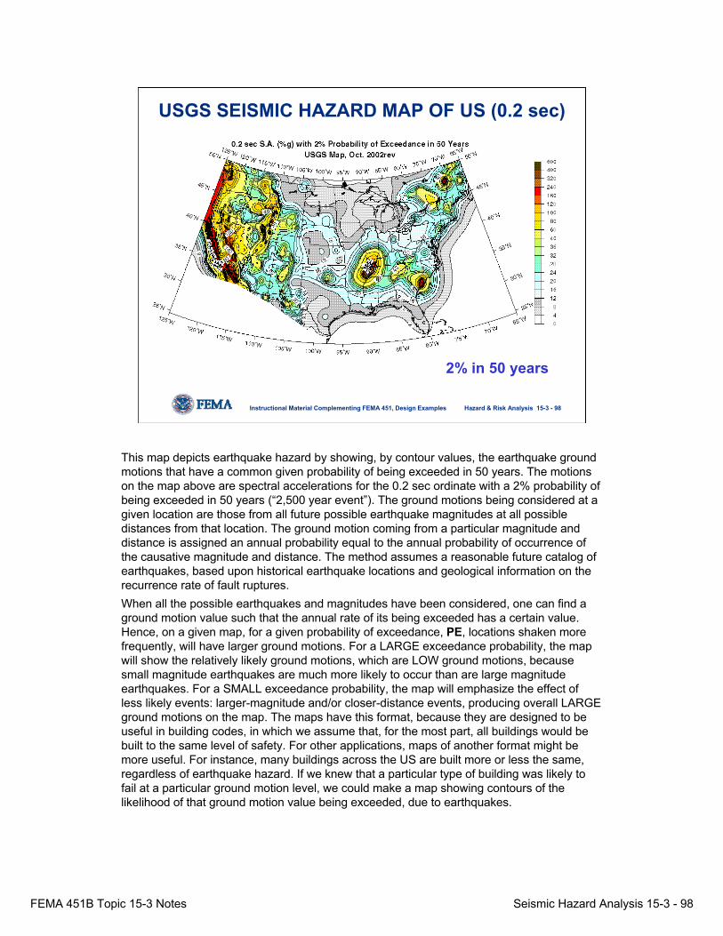
FEMA 451B Topic 15-3 Notes Seismic Hazard Analysis 15-3 - 98
Hazard & Risk Analysis 15-3 - 98Instructional Material Complementing FEMA 451, Design Examples
USGS SEISMIC HAZARD MAP OF US (0.2 sec)
2% in 50 years
This map depicts earthquake hazard by showing, by contour values, the earthquake ground motions that have a common given probability of being exceeded in 50 years. The motions on the map above are spectral accelerations for the 0.2 sec ordinate with a 2% probability of being exceeded in 50 years (“2,500 year event”). The ground motions being considered at a given location are those from all future possible earthquake magnitudes at all possible distances from that location. The ground motion coming from a particular magnitude and distance is assigned an annual probability equal to the annual probability of occurrence of the causative magnitude and distance. The method assumes a reasonable future catalog of earthquakes, based upon historical earthquake locations and geological information on the recurrence rate of fault ruptures.When all the possible earthquakes and magnitudes have been considered, one can find a ground motion value such that the annual rate of its being exceeded has a certain value. Hence, on a given map, for a given probability of exceedance, PE, locations shaken more frequently, will have larger ground motions. For a LARGE exceedance probability, the map will show the relatively likely ground motions, which are LOW ground motions, because small magnitude earthquakes are much more likely to occur than are large magnitude earthquakes. For a SMALL exceedance probability, the map will emphasize the effect of less likely events: larger-magnitude and/or closer-distance events, producing overall LARGE ground motions on the map. The maps have this format, because they are designed to be useful in building codes, in which we assume that, for the most part, all buildings would be built to the same level of safety. For other applications, maps of another format might be more useful. For instance, many buildings across the US are built more or less the same, regardless of earthquake hazard. If we knew that a particular type of building was likely to fail at a particular ground motion level, we could make a map showing contours of the likelihood of that ground motion value being exceeded, due to earthquakes.

FEMA 451B Topic 15-3 Notes Seismic Hazard Analysis 15-3 - 99
Hazard & Risk Analysis 15-3 - 99Instructional Material Complementing FEMA 451, Design Examples
USGS SEISMIC HAZARD MAP OF US (1.0 sec)
2% in 50 years
This map depicts earthquake hazard by showing, by contour values, the earthquake ground motions that have a common given probability of being exceeded in 50 years. The motions on the map above are spectral accelerations for the 1.0 sec ordinate with a 2% probability of being exceeded in 50 years (“2,500 year event”). The ground motions being considered at a given location are those from all future possible earthquake magnitudes at all possible distances from that location. The ground motion coming from a particular magnitude and distance is assigned an annual probability equal to the annual probability of occurrence of the causative magnitude and distance. The method assumes a reasonable future catalog of earthquakes, based upon historical earthquake locations and geological information on the recurrence rate of fault ruptures.When all the possible earthquakes and magnitudes have been considered, one can find a ground motion value such that the annual rate of its being exceeded has a certain value. Hence, on a given map, for a given probability of exceedance, PE, locations shaken more frequently, will have larger ground motions. For a LARGE exceedance probability, the map will show the relatively likely ground motions, which are LOW ground motions, because small magnitude earthquakes are much more likely to occur than are large magnitude earthquakes. For a SMALL exceedance probability, the map will emphasize the effect of less likely events: larger-magnitude and/or closer-distance events, producing overall LARGE ground motions on the map. The maps have this format, because they are designed to be useful in building codes, in which we assume that, for the most part, all buildings would be built to the same level of safety. For other applications, maps of another format might be more useful. For instance, many buildings across the US are built more or less the same, regardless of earthquake hazard. If we knew that a particular type of building was likely to fail at a particular ground motion level, we could make a map showing contours of the likelihood of that ground motion value being exceeded, due to earthquakes.
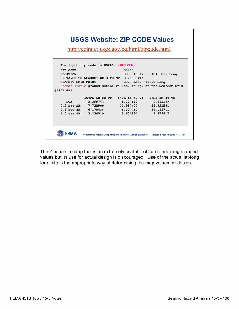
FEMA 451B Topic 15-3 Notes Seismic Hazard Analysis 15-3 - 100
Hazard & Risk Analysis 15-3 - 100Instructional Material Complementing FEMA 451, Design Examples
The input zip-code is 80203. (DENVER)ZIP CODE 80203LOCATION 39.7310 Lat. -104.9815 Long.DISTANCE TO NEAREST GRID POINT 3.7898 kmsNEAREST GRID POINT 39.7 Lat. -105.0 Long.Probabilistic ground motion values, in %g, at the Nearest Grid
point are:
10%PE in 50 yr 5%PE in 50 yr 2%PE in 50 yrPGA 3.299764 5.207589 9.642159
0.2 sec SA 7.728900 11.917400 19.9215910.3 sec SA 6.178438 9.507714 16.1337111.0 sec SA 2.334019 3.601994 5.879917
http://eqint.cr.usgs.gov/eq/html/zipcode.htmlUSGS Website: ZIP CODE Values
The Zipcode Lookup tool is an extremely useful tool for determining mapped values but its use for actual design is discouraged. Use of the actual lat-long for a site is the appropriate way of determining the map values for design.

FEMA 451B Topic 15-3 Notes Seismic Hazard Analysis 15-3 - 101
Hazard & Risk Analysis 15-3 - 101Instructional Material Complementing FEMA 451, Design Examples
USGS Seismic Hazard Maps• Hazard in some areas increased relative to
previous maps due to recent studies.• Maps developed for motions on B-C soil
boundary (soft rock).• Maps do not account for regional geological
effects such as deep profiles of unconsolidated sediments– this is big effect in CEUS (i.e., in Charleston ~1 km thick).
• New 2002 versions of maps revised in April 2003.
None.

FEMA 451B Topic 15-3 Notes Seismic Hazard Analysis 15-3 - 102
Hazard & Risk Analysis 15-3 - 102Instructional Material Complementing FEMA 451, Design Examples
National Seismic Hazard Maps Uses:• can illustrate relative probability of a given level of
earthquake ground motion of one part of the country relative to another.
• illustrate the relative demand on structures in one region relative to another, at a given probability level.
• as per building codes, use maps as benchmark to determine the resistance required by buildings to resist damaging levels of ground motion.
• with judgment and sometimes special procedures, use maps to determine the input ground motions for geotechnical earthquake analyses (liquefaction,etc.)
None.

FEMA 451B Topic 15-3 Notes Seismic Hazard Analysis 15-3 - 103
Hazard & Risk Analysis 15-3 - 103Instructional Material Complementing FEMA 451, Design Examples
USGS Seismic Hazard Curves for Various Cities
Note differences between 500-yr and 2,500-yr EQ’s
Due to the shape of the hazard curves, it can be seen that in the EUS, there is great difference between the 500 and 2,500-year event. Thus, this left many buildings in the CEUS designed for the 500-year event vulnerable to collapse in a large, rare earthquake (i.e., 2500-year event). New IBC2003 Code provisions account for this by using 2,500-year event (MCE) as the basis for design in all regions.

FEMA 451B Topic 15-3 Notes Seismic Hazard Analysis 15-3 - 104
Hazard & Risk Analysis 15-3 - 104Instructional Material Complementing FEMA 451, Design Examples
Large earthquakes rare
How Does CEUS and WUS Seismic Risk Compare?
Large earthquakes frequent vs.
People are different, so what about earthquakes? Large, damagingearthquakes occur more frequently in the western US and thus the seismic hazard is higher there, but this is not true for the overall seismic risk because the consequences of such an event are much greater in the eastern US due to the weaker infrastructure and lower attenuation. Large, damaging earthquakes occur more frequently in the western US and thus the seismic hazard is higher there, but this is not true for the overall seismic risk because the consequences of such an event are much greater in the eastern US due to the weaker infrastructure and lower attenuation.

FEMA 451B Topic 15-3 Notes Seismic Hazard Analysis 15-3 - 105
Hazard & Risk Analysis 15-3 - 105Instructional Material Complementing FEMA 451, Design Examples
1886 Charleston Earthquake Felt Over EUS!
New York >600 mi.
Charleston
St. Louis > 650 mi.
Chicago > 700 mi.
The 1886 Charleston earthquake was felt over an unusually long distance (relative to west-coast standards). Again, this reflects the lower attenuation in this region due to harder rock.

FEMA 451B Topic 15-3 Notes Seismic Hazard Analysis 15-3 - 106
Hazard & Risk Analysis 15-3 - 106Instructional Material Complementing FEMA 451, Design Examples
WUS vs. CEUS Attenuation
compare
compare
Attenuation is lower in CEUS because of location in the middle of plate. Crust is older, colder, and much harder than in the WUS.
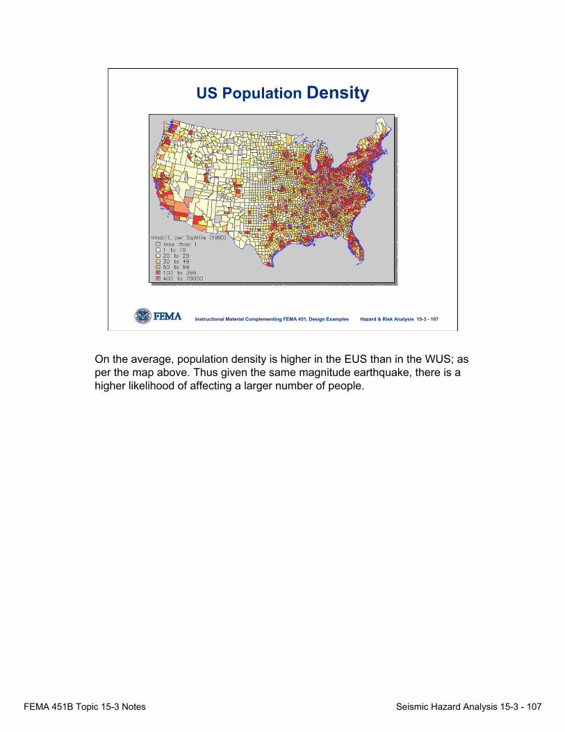
FEMA 451B Topic 15-3 Notes Seismic Hazard Analysis 15-3 - 107
Hazard & Risk Analysis 15-3 - 107Instructional Material Complementing FEMA 451, Design Examples
US Population Density
On the average, population density is higher in the EUS than in the WUS; as per the map above. Thus given the same magnitude earthquake, there is a higher likelihood of affecting a larger number of people.
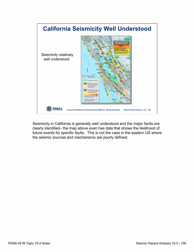
FEMA 451B Topic 15-3 Notes Seismic Hazard Analysis 15-3 - 108
Hazard & Risk Analysis 15-3 - 108Instructional Material Complementing FEMA 451, Design Examples
California Seismicity Well Understood
Seismicity relatively well understood
Seismicity in California is generally well understood and the major faults are clearly identified– the map above even has data that shows the likelihood of future events for specific faults. This is not the case in the eastern US where the seismic sources and mechanisms are poorly defined.

FEMA 451B Topic 15-3 Notes Seismic Hazard Analysis 15-3 - 109
Hazard & Risk Analysis 15-3 - 109Instructional Material Complementing FEMA 451, Design Examples
Seismically Weak Infrastructure in CEUS
There is an abundance of seismically weak infrastructure in the CEUS. Figure above shows damage to an unreinforced masonry structure near 6th
and Townsend Streets during the 1989 Loma Prieta earthquake. Close-up photos on the right show cars that were crushed leading to the death of five people. This building was located in the western US, but similar construction is abundant in the central and eastern US.

FEMA 451B Topic 15-3 Notes Seismic Hazard Analysis 15-3 - 110
Hazard & Risk Analysis 15-3 - 110Instructional Material Complementing FEMA 451, Design Examples
WUS and CEUS Risk Comparison• CEUS has potential for recurring large
earthquakes • Attenuation lower in CEUS• Weak structures not “weeded out” in CEUS• “Adolescent” seismic practice in CEUS• “Human inertia” in CEUS• Much more uncertainty in CEUS
• Bottom line ⇒ seismic risk in CEUS and WUS is comparable!
The seismic risk is higher in the WUS due to the higher frequency of earthquakes, but the risk in the EUS is comparable.
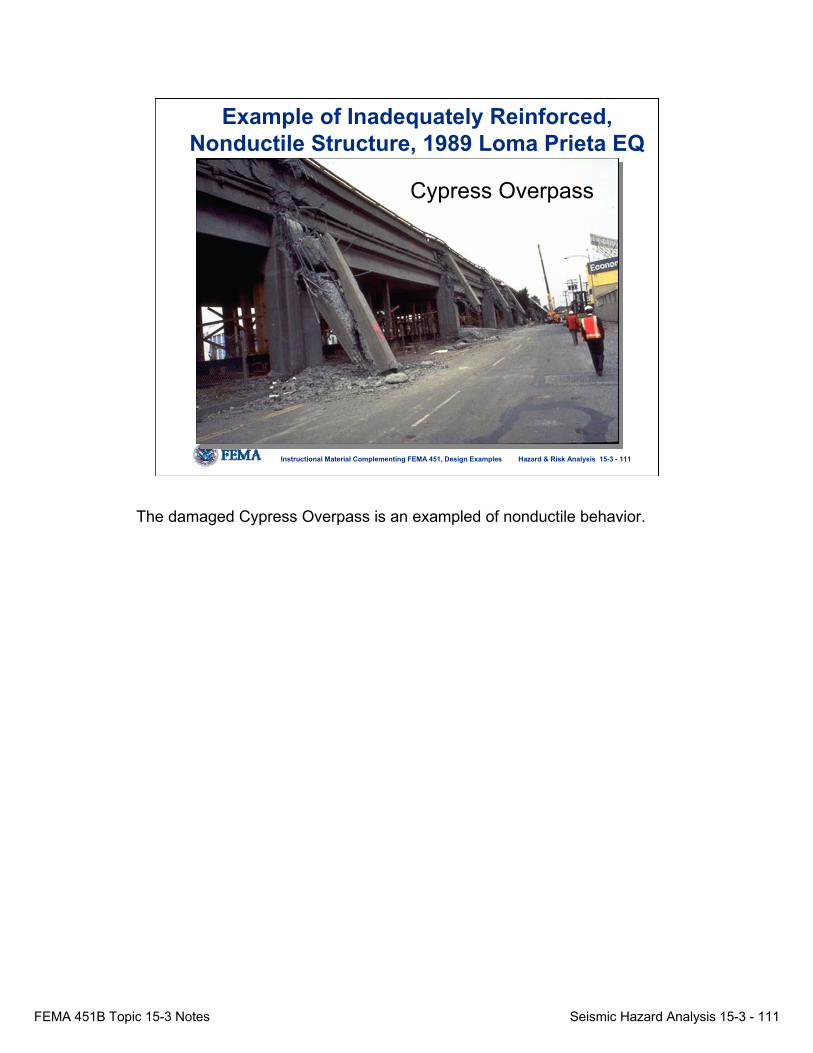
FEMA 451B Topic 15-3 Notes Seismic Hazard Analysis 15-3 - 111
Hazard & Risk Analysis 15-3 - 111Instructional Material Complementing FEMA 451, Design Examples
Example of Inadequately Reinforced, Nonductile Structure, 1989 Loma Prieta EQ
Cypress Overpass
The damaged Cypress Overpass is an exampled of nonductile behavior.

FEMA 451B Topic 15-3 Notes Seismic Hazard Analysis 15-3 - 112
Hazard & Risk Analysis 15-3 - 112Instructional Material Complementing FEMA 451, Design Examples
The poor performance of the Cypress Structure prompted the decision to tear down the rest of the structure following the 1989 Loma Prieta earthquake.

FEMA 451B Topic 15-3 Notes Seismic Hazard Analysis 15-3 - 113
Hazard & Risk Analysis 15-3 - 113Instructional Material Complementing FEMA 451, Design Examples

FEMA 451B Topic 15-3 Notes Seismic Hazard Analysis 15-3 - 114
Hazard & Risk Analysis 15-3 - 114Instructional Material Complementing FEMA 451, Design Examples

FEMA 451B Topic 15-3 Notes Seismic Hazard Analysis 15-3 - 115
Hazard & Risk Analysis 15-3 - 115Instructional Material Complementing FEMA 451, Design Examples
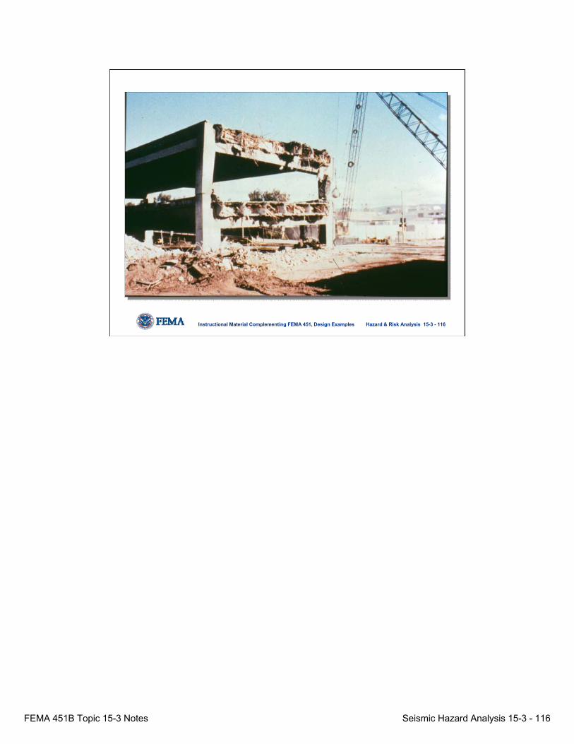
FEMA 451B Topic 15-3 Notes Seismic Hazard Analysis 15-3 - 116
Hazard & Risk Analysis 15-3 - 116Instructional Material Complementing FEMA 451, Design Examples

FEMA 451B Topic 15-3 Notes Seismic Hazard Analysis 15-3 - 117
Hazard & Risk Analysis 15-3 - 117Instructional Material Complementing FEMA 451, Design Examples

FEMA 451B Topic 15-3 Notes Seismic Hazard Analysis 15-3 - 118
Hazard & Risk Analysis 15-3 - 118Instructional Material Complementing FEMA 451, Design Examples
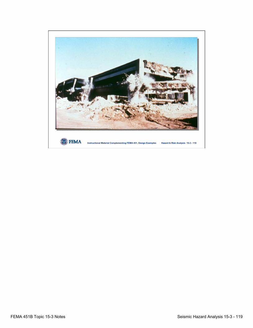
FEMA 451B Topic 15-3 Notes Seismic Hazard Analysis 15-3 - 119
Hazard & Risk Analysis 15-3 - 119Instructional Material Complementing FEMA 451, Design Examples

FEMA 451B Topic 15-3 Notes Seismic Hazard Analysis 15-3 - 120
Hazard & Risk Analysis 15-3 - 120Instructional Material Complementing FEMA 451, Design Examples
This Type of Non-Ductile Infrastructure is Common in CEUS!
This collapse was cause by one impact of the wrecking ball! Again, classic nonductile behavior.
FEMA 451B Topic 15-3 Notes Seismic Hazard Analysis 15-3 - 121
Hazard & Risk Analysis 15-3 - 121Instructional Material Complementing FEMA 451, Design Examples
WUS and CEUS Risk Comparison Summary• CEUS has potential for recurring large EQs• Attenuation lower in CEUS• Abundance of weak, non-ductile structures in CEUS;
weakest not “weeded out”• Immature seismic practice in CEUS• “Human inertia” in CEUS; little awareness• Much more uncertainty in CEUS• Areas with poor soils in CEUS
• Bottom line ⇒ seismic risk in CEUS and WUS is comparable!
The comparable seismic risks between WUS and CEUS are surprising to many.

FEMA 451B Topic 15-3 Notes Seismic Hazard Analysis 15-3 - 122
Hazard & Risk Analysis 15-3 - 122Instructional Material Complementing FEMA 451, Design Examples
Issues To Think About
• Good analogy ⇒ Kobe is to Tokyo, as CEUS is to the WUS
• Kobe M6.9 (> $120 billion losses); weaker infrastructure, poor soil conditions
• Remember ⇒ most expensive US natural disaster (Northridge, EQ ∼$30 billion) was moderate earthquake on minor fault on fringe of Los Angeles
The fact that the most expensive US natural disaster (Northridge, California, earthquake ∼$30 billion) was a moderate earthquake on minor fault on the fringe of Los Angeles is alarming in terms of demonstrating the damage potential of earthquakes.
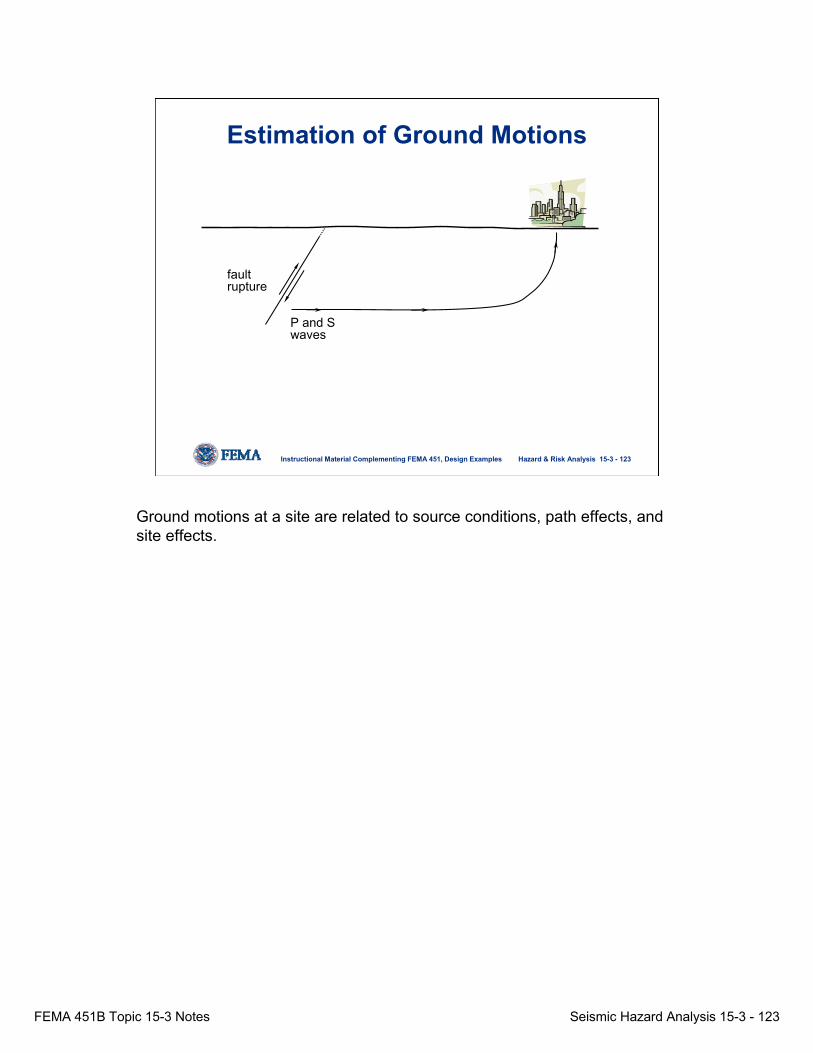
FEMA 451B Topic 15-3 Notes Seismic Hazard Analysis 15-3 - 123
Hazard & Risk Analysis 15-3 - 123Instructional Material Complementing FEMA 451, Design Examples
Estimation of Ground Motions
fault rupture
P and S waves
Ground motions at a site are related to source conditions, path effects, and site effects.
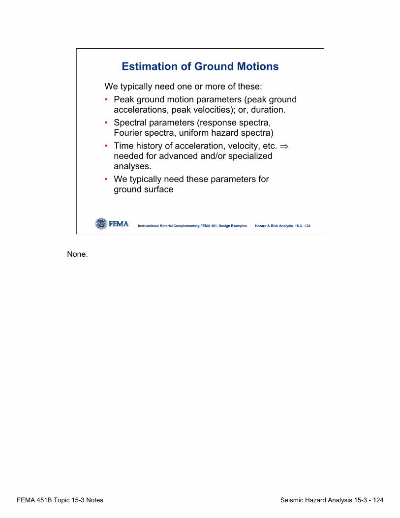
FEMA 451B Topic 15-3 Notes Seismic Hazard Analysis 15-3 - 124
Hazard & Risk Analysis 15-3 - 124Instructional Material Complementing FEMA 451, Design Examples
Estimation of Ground Motions
We typically need one or more of these: • Peak ground motion parameters (peak ground
accelerations, peak velocities); or, duration.• Spectral parameters (response spectra,
Fourier spectra, uniform hazard spectra)• Time history of acceleration, velocity, etc. ⇒
needed for advanced and/or specialized analyses.
• We typically need these parameters for ground surface
None.
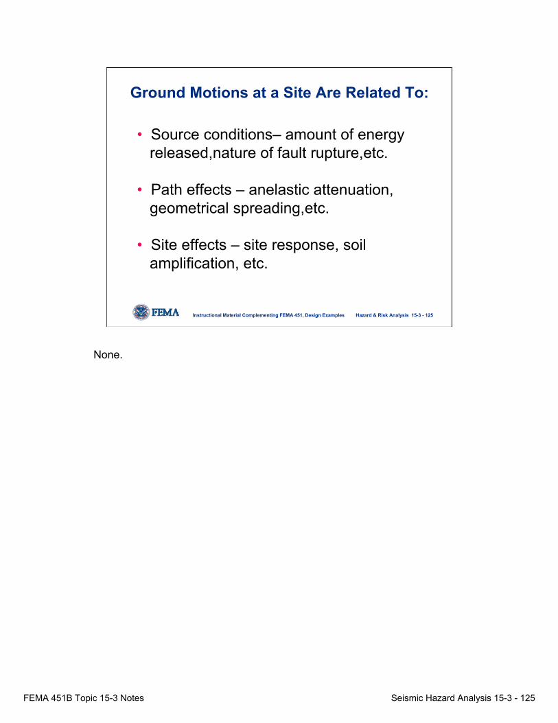
FEMA 451B Topic 15-3 Notes Seismic Hazard Analysis 15-3 - 125
Hazard & Risk Analysis 15-3 - 125Instructional Material Complementing FEMA 451, Design Examples
Ground Motions at a Site Are Related To:
• Source conditions– amount of energyreleased,nature of fault rupture,etc.
• Path effects – anelastic attenuation, geometrical spreading,etc.
• Site effects – site response, soil amplification, etc.
None.

FEMA 451B Topic 15-3 Notes Seismic Hazard Analysis 15-3 - 126
Hazard & Risk Analysis 15-3 - 126Instructional Material Complementing FEMA 451, Design Examples
Source Conditions Include:• Stress drop• Source depth• Size of the rupture area • Slip distribution (amount and distribution of
static displacement on the fault plane) • Rise time (time for the fault slip to
complete at a given point on the fault plane)
• Type of faulting • Rupture directivity
None.
FEMA 451B Topic 15-3 Notes Seismic Hazard Analysis 15-3 - 127
Hazard & Risk Analysis 15-3 - 127Instructional Material Complementing FEMA 451, Design Examples
Transmission Path Includes:
• Crustal structure
• Shear-wave velocity (or Q) and damping characteristics of the crustal rock
None.

FEMA 451B Topic 15-3 Notes Seismic Hazard Analysis 15-3 - 128
Hazard & Risk Analysis 15-3 - 128Instructional Material Complementing FEMA 451, Design Examples
Site Conditions Include:
• Rock properties beneath the site to depths of up to about 2 km (hard crystalline rock)
• Local soil conditions at the site to depths of up to several hundred feet (typically)
• Topography of the site
Local soil conditions at a site usually involves material with depths of up to several hundred feet (typically) – 30 m is more or less common value.

FEMA 451B Topic 15-3 Notes Seismic Hazard Analysis 15-3 - 129
Hazard & Risk Analysis 15-3 - 129Instructional Material Complementing FEMA 451, Design Examples
Effects of Magnitude
From USACE, 2000
The larger the magnitude, the longer the duration of motion and the larger the amplitude of motion (up to a point). United States Army Corps of Engineers (USACE) (2000). “Time history of dynamic analsyis of concrete hydraulic structures,” Engineering Circular (EC) 1110-2-6051, Department of the Army, Washington, D.C.
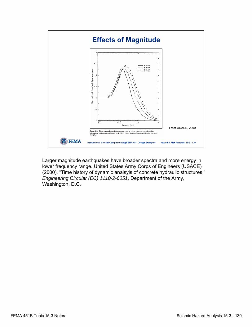
FEMA 451B Topic 15-3 Notes Seismic Hazard Analysis 15-3 - 130
Hazard & Risk Analysis 15-3 - 130Instructional Material Complementing FEMA 451, Design Examples
Effects of Magnitude
From USACE, 2000
Larger magnitude earthquakes have broader spectra and more energy in lower frequency range. United States Army Corps of Engineers (USACE) (2000). “Time history of dynamic analsyis of concrete hydraulic structures,”Engineering Circular (EC) 1110-2-6051, Department of the Army, Washington, D.C.
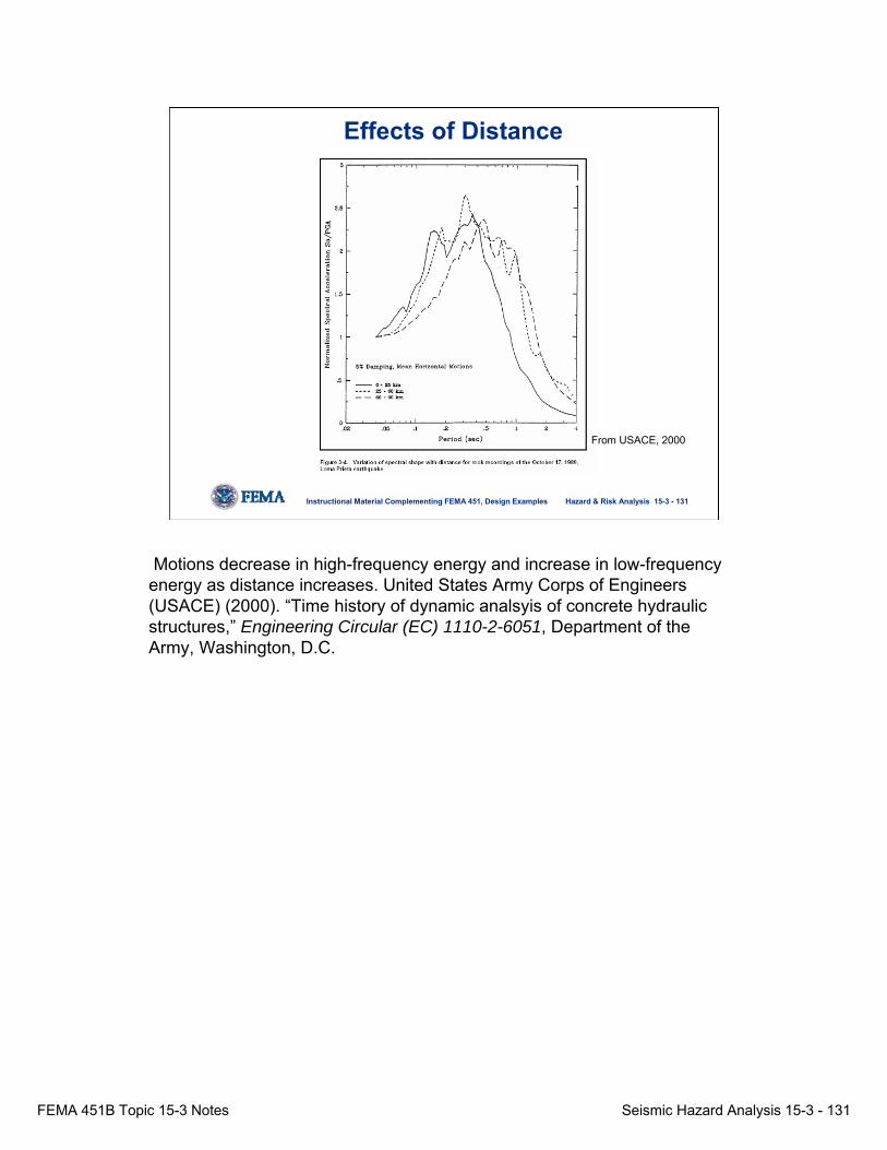
FEMA 451B Topic 15-3 Notes Seismic Hazard Analysis 15-3 - 131
Hazard & Risk Analysis 15-3 - 131Instructional Material Complementing FEMA 451, Design Examples
Effects of Distance
From USACE, 2000
Motions decrease in high-frequency energy and increase in low-frequency energy as distance increases. United States Army Corps of Engineers (USACE) (2000). “Time history of dynamic analsyis of concrete hydraulic structures,” Engineering Circular (EC) 1110-2-6051, Department of the Army, Washington, D.C.

FEMA 451B Topic 15-3 Notes Seismic Hazard Analysis 15-3 - 132
Hazard & Risk Analysis 15-3 - 132Instructional Material Complementing FEMA 451, Design Examples
Effects of Distance
From USACE, 2000
Motions decrease in high-frequency energy and increase in low-frequency energy as distance increases. United States Army Corps of Engineers (USACE) (2000). “Time history of dynamic analsyis of concrete hydraulic structures,” Engineering Circular (EC) 1110-2-6051, Department of the Army, Washington, D.C.
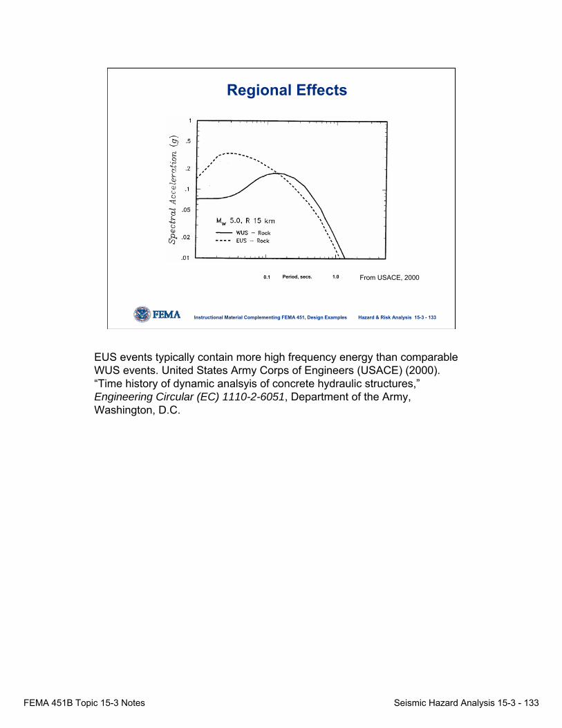
FEMA 451B Topic 15-3 Notes Seismic Hazard Analysis 15-3 - 133
Hazard & Risk Analysis 15-3 - 133Instructional Material Complementing FEMA 451, Design Examples
Regional Effects
0.1 1.0Period, secs. From USACE, 2000
EUS events typically contain more high frequency energy than comparable WUS events. United States Army Corps of Engineers (USACE) (2000). “Time history of dynamic analsyis of concrete hydraulic structures,”Engineering Circular (EC) 1110-2-6051, Department of the Army, Washington, D.C.

FEMA 451B Topic 15-3 Notes Seismic Hazard Analysis 15-3 - 134
Hazard & Risk Analysis 15-3 - 134Instructional Material Complementing FEMA 451, Design Examples
Effect of Local Site Conditions
Figure adapted from Seed and Idriss (1984); EERI.
Soft soils decrease the spectral response relative to some stiff soils, but the range over which the motions are near their maximum is broadened.

FEMA 451B Topic 15-3 Notes Seismic Hazard Analysis 15-3 - 135
Hazard & Risk Analysis 15-3 - 135Instructional Material Complementing FEMA 451, Design Examples
Special Near-source Effects
“Near-source” can be interpreted differently. For many engineering applications, a zone within about 20 km of the fault rupture is considered near-source. Other cases near-source is considered within a distance roughly equal to the ruptured length of the fault; 20 to 60 km typical
Near-source effects:• Directiviity• Fling• Radiation pattern
“Near-source” can be interpreted differently. For many engineering applications, a zone within about 20 km of the fault rupture is considered near-source. Other cases near-source is considered within a distance roughly equal to the ruptured length of the fault; 20 to 60 km typical

FEMA 451B Topic 15-3 Notes Seismic Hazard Analysis 15-3 - 136
Hazard & Risk Analysis 15-3 - 136Instructional Material Complementing FEMA 451, Design Examples
Two Causes of large velocity pulses:
• Directivity • Fling
Important Near-Fault Effects
Directivity is related to the direction of the rupture front and fling is related to permanent tectonic deformation.
FEMA 451B Topic 15-3 Notes Seismic Hazard Analysis 15-3 - 137
Hazard & Risk Analysis 15-3 - 137Instructional Material Complementing FEMA 451, Design Examples
Directivity: • Related to the direction of the rupture
front – Forward directivity: rupture toward the site
(site away from the epicenter) – Backward directivity: rupture away from the site
(site near the epicenter)
Fling: • Related to the permanent tectonic
deformation at the site
Causes of Velocity Pulses
None.
FEMA 451B Topic 15-3 Notes Seismic Hazard Analysis 15-3 - 138
Hazard & Risk Analysis 15-3 - 138Instructional Material Complementing FEMA 451, Design Examples
• Directivity – Two-sided velocity pulse due to constructive
interference of SH waves from generated from parts of the rupture located between the site and epicenter; affects fault-normal component
– Occurs at sites located close to the fault but away from the epicenter
• Fling – One-sided velocity pulse due to tectonic
deformation; affects fault-parallel component – Occurs at sites located near the fault rupture
independent of the epicenter location
Velocity Pulses
Both directivity and fling increase ground motions and seismic demand on structures.

FEMA 451B Topic 15-3 Notes Seismic Hazard Analysis 15-3 - 139
Hazard & Risk Analysis 15-3 - 139Instructional Material Complementing FEMA 451, Design Examples
-150
0
150
0 2 4 6 8 10 12
Dis
p (c
m)
Time (sec)
-0.1
0
0.1
0 2 4 6 8 10 12
Acc
(g)
Time (sec)
-80
-40
0
40
80
0 2 4 6 8 10 12
Vel
(cm
/s)
Time (sec)
Preliminary Model for Fling
Figure adapted from Abrahamson at http://civil.eng.buffalo.edu/webcast/abrahamson/presentation_files/frame.htm
The large displacement (static) shown at about 6 seconds (bottom) corresponds to the large velocity (and acceleration) pulse that occurs in the record motions.

FEMA 451B Topic 15-3 Notes Seismic Hazard Analysis 15-3 - 140
Hazard & Risk Analysis 15-3 - 140Instructional Material Complementing FEMA 451, Design Examples
QGa
-200
0
200
0 5 10 15 20 25 30 35 40
Dis
p (c
m)
Time (sec)
-0.9
0
0.9
0 5 10 15 20 25 30 35 40
Acc(
g)
Time (sec)
-200
0
200
0 5 10 15 20 25 30 35 40
Vel (
cm/s
)
Time (sec)
Vibratory Ground Motion + Fling
Figure adapted from Abrahamson at http://civil.eng.buffalo.edu/webcast/abrahamson/presentation_files/frame.htm
The large displacement shown at about 10 seconds (bottom) corresponds to the large velocity (and acceleration) pulse that occurs in the record motions.

FEMA 451B Topic 15-3 Notes Seismic Hazard Analysis 15-3 - 141
Hazard & Risk Analysis 15-3 - 141Instructional Material Complementing FEMA 451, Design Examples
-0.25
0
0.25
0.5
30 35 40 45 50 55 60
Acc
(g)
flingTCU052E
-200-150-100-50
050
100
30 35 40 45 50 55 60
Vel
(cm
/s)
flingTCU052E
-500-400-300-200-100
0100
30 35 40 45 50 55 60
Dis
(cm
)
Time (sec)
flingTCU052E
TCU052 (1999 Chi-Chi)
Figure adapted from Abrahamson at http://civil.eng.buffalo.edu/webcast/abrahamson/presentation_files/frame.htm
FEMA 451B Topic 15-3 Notes Seismic Hazard Analysis 15-3 - 142
Hazard & Risk Analysis 15-3 - 142Instructional Material Complementing FEMA 451, Design Examples
• Not currently known which types of structures are sensitive to fling ground motions.
• Preliminary results indicate some long-span structure may be sensitive to fling.
• Need to evaluate various types of structures to ground motions with and without fling to determine the effect.
Effects of Fling
In strike slip faulting, the fling affects the strike-parallel component of ground motion.

FEMA 451B Topic 15-3 Notes Seismic Hazard Analysis 15-3 - 143
Hazard & Risk Analysis 15-3 - 143Instructional Material Complementing FEMA 451, Design Examples
Forward directivity
Backward directivity
Rupture direction
Rupture direction
The areas under the far-field displacementpulses are equal, but the amplitudesand durations differ. This has majoreffects on the ground velocity and acceleration.
Ground Displacement
To Receiver
To Receiver
Figure above adapted from Martin Chapman, Virginia Tech Department of Geological Sciences. The effect of directivity is prominent in the fault parallel direction (i.e., in direction of fault rupture) but affects the fault perpendicular component of the ground motion. For instance, in strike slip faulting, the directivity pulse occurs on the strike normal component.
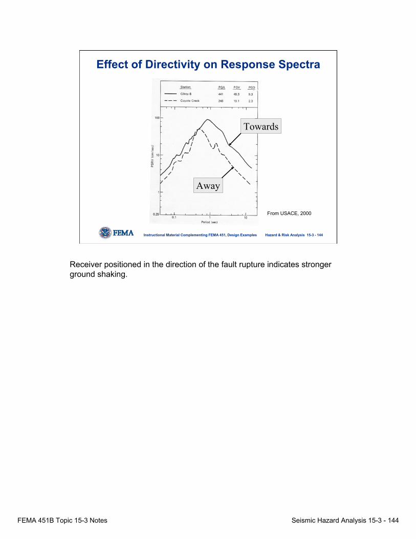
FEMA 451B Topic 15-3 Notes Seismic Hazard Analysis 15-3 - 144
Hazard & Risk Analysis 15-3 - 144Instructional Material Complementing FEMA 451, Design Examples
Towards
Away
Effect of Directivity on Response Spectra
From USACE, 2000
Receiver positioned in the direction of the fault rupture indicates stronger ground shaking.
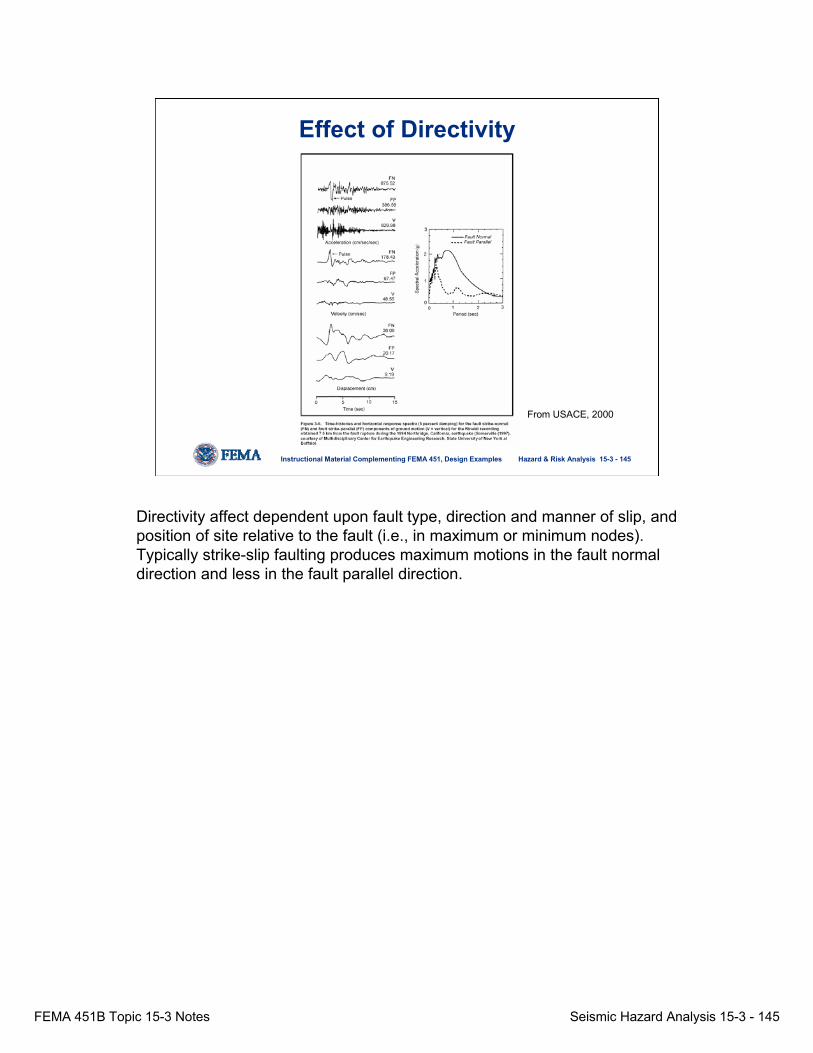
FEMA 451B Topic 15-3 Notes Seismic Hazard Analysis 15-3 - 145
Hazard & Risk Analysis 15-3 - 145Instructional Material Complementing FEMA 451, Design Examples
Effect of Directivity
From USACE, 2000
Directivity affect dependent upon fault type, direction and manner of slip, and position of site relative to the fault (i.e., in maximum or minimum nodes). Typically strike-slip faulting produces maximum motions in the fault normal direction and less in the fault parallel direction.

FEMA 451B Topic 15-3 Notes Seismic Hazard Analysis 15-3 - 146
Hazard & Risk Analysis 15-3 - 146Instructional Material Complementing FEMA 451, Design Examples
• Directivity can cause amplification of motions for sites close to the fault rupture.
• Unclear as to engineering significance of fling.
• Current attenuation relations do not include these effects.
Effects of Fling and Directivity
Both directivity and fling are difficult to predict precise and design for using simplified methods.

FEMA 451B Topic 15-3 Notes Seismic Hazard Analysis 15-3 - 147
Hazard & Risk Analysis 15-3 - 147Instructional Material Complementing FEMA 451, Design Examples
rupture direction
Fault normal componentIn the direction of forwarddirectivity.
Fault normal component
Point SourceFinite Source
Fault parallel component
Fault Plane
SH Radiation Pattern for Vertical Strike-slip
Illustration of directivity effects. Figure indicates type of energy radiation associated with each point along the fault. Lobes of energy radiation indicates predicted motions along the fault in direction of rupture. The pattern of energy radiation shown for a point along the fault is same as what overall energy pattern looks like when the fault is view from a very large scale such that it look like a point source.

FEMA 451B Topic 15-3 Notes Seismic Hazard Analysis 15-3 - 148
Hazard & Risk Analysis 15-3 - 148Instructional Material Complementing FEMA 451, Design Examples
Other Important Effects• Also, vertical motions tend to be higher
than 2/3 maximum horizontal motions when near-source.
• Subduction zone EQs vs. shallow EQs• Topographical effects (especially
basins).• Surface waves may be important for
certain long-span structures (relative motion among supports).
• Others…
Other special situations require more advanced analyses (rather than simplified without careful consideration).
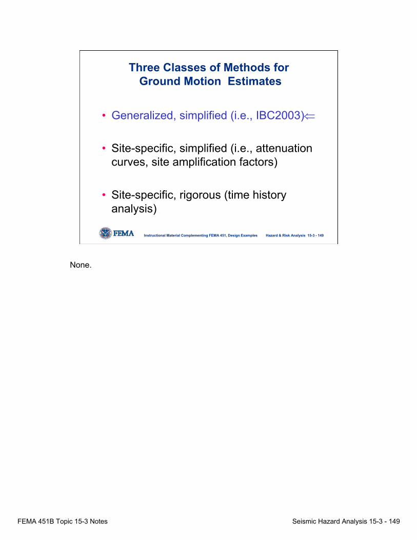
FEMA 451B Topic 15-3 Notes Seismic Hazard Analysis 15-3 - 149
Hazard & Risk Analysis 15-3 - 149Instructional Material Complementing FEMA 451, Design Examples
Three Classes of Methods forGround Motion Estimates
• Generalized, simplified (i.e., IBC2003)⇐
• Site-specific, simplified (i.e., attenuation curves, site amplification factors)
• Site-specific, rigorous (time history analysis)
None.

FEMA 451B Topic 15-3 Notes Seismic Hazard Analysis 15-3 - 150
Hazard & Risk Analysis 15-3 - 150Instructional Material Complementing FEMA 451, Design Examples
Generalized, Simplified (i.e., IBC 2003)
• Simple to use.• Based on probabilistic maps.• Does not account for regional geological effects
(maps assume standard depth for B-C boundary and profile layering) ⇒ in WUS, B-C boundary is shallow bedrock, but in some CEUS areas the B-C boundary is deep as 1 km.
• Accounts for local site effects in general manner– cannot handle special site conditions.
• Not well-suited to many geotechnical analyses (no magnitude, UHS approach, etc.).
Most generalized methods, such as those used by building codes do not account for regional geological effects (maps assume standard depth for B-C boundary and profile layering)⇒ in WUS, B-C boundary is typically shallow bedrock, but in some CEUS areas the B-C boundary is deep as 1 km.

FEMA 451B Topic 15-3 Notes Seismic Hazard Analysis 15-3 - 151
Hazard & Risk Analysis 15-3 - 151Instructional Material Complementing FEMA 451, Design Examples
IBC 2003 - Overview• Developed from a combination of three legacy
model codes (UBC, BOCA, & SBC).• Based largely on FEMA 368 and 369, NEHRP
Recommended Provisions and Commentary.• Adopted in 45 states (as of July 2004) and by
the DoD.• Incorporates most recent (2002/2003) USGS
seismic hazard maps; USGS map values capped in some areas by IBC 2003.
IBC2003 incorporates the most recent (2002/2003) USGS seismic hazard maps, but the IBC caps the USGS map values in some areas (i.e., southern California) so the IBC2003 values are lower than the USGS maps. In most other states, the USGS and IBC maps are exact.
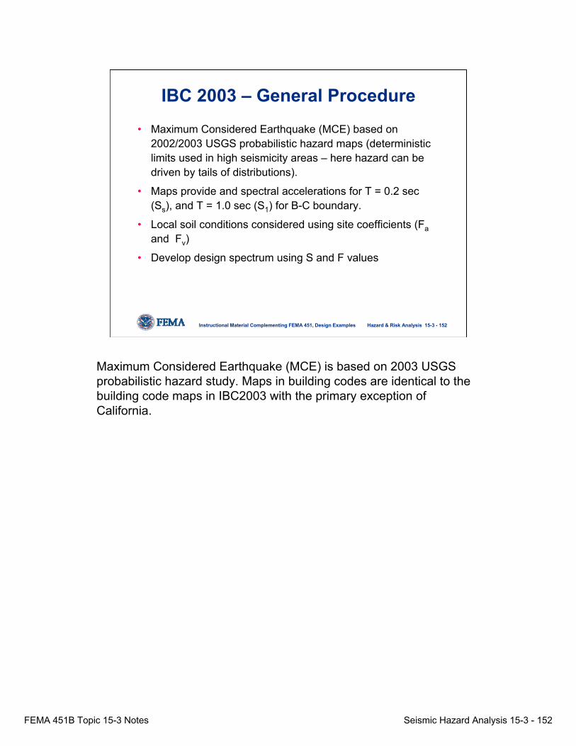
FEMA 451B Topic 15-3 Notes Seismic Hazard Analysis 15-3 - 152
Hazard & Risk Analysis 15-3 - 152Instructional Material Complementing FEMA 451, Design Examples
IBC 2003 – General Procedure
• Maximum Considered Earthquake (MCE) based on 2002/2003 USGS probabilistic hazard maps (deterministic limits used in high seismicity areas – here hazard can be driven by tails of distributions).
• Maps provide and spectral accelerations for T = 0.2 sec (Ss), and T = 1.0 sec (S1) for B-C boundary.
• Local soil conditions considered using site coefficients (Fa and Fv)
• Develop design spectrum using S and F values
Maximum Considered Earthquake (MCE) is based on 2003 USGS probabilistic hazard study. Maps in building codes are identical to the building code maps in IBC2003 with the primary exception of California.
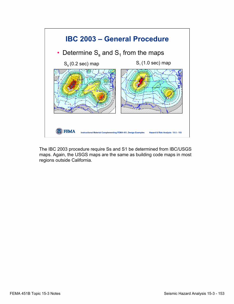
FEMA 451B Topic 15-3 Notes Seismic Hazard Analysis 15-3 - 153
Hazard & Risk Analysis 15-3 - 153Instructional Material Complementing FEMA 451, Design Examples
IBC 2003 – General Procedure
• Determine Ss and S1 from the mapsSs (0.2 sec) map S1 (1.0 sec) map
The IBC 2003 procedure require Ss and S1 be determined from IBC/USGS maps. Again, the USGS maps are the same as building code maps in most regions outside California.

FEMA 451B Topic 15-3 Notes Seismic Hazard Analysis 15-3 - 154
Hazard & Risk Analysis 15-3 - 154Instructional Material Complementing FEMA 451, Design Examples
IBC 2003 – General Procedure• Determine site class based on top 30 m:
Note special provisions for “F” sites. These site conditions are of particular concern for seismic analysis. F site involved soft soils that can greatly amplify ground motions, such as in Mexico City in 1985 or Loma Prieta in 1989 or liquefiable soils.
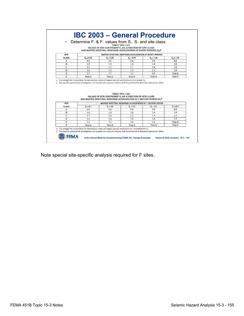
FEMA 451B Topic 15-3 Notes Seismic Hazard Analysis 15-3 - 155
Hazard & Risk Analysis 15-3 - 155Instructional Material Complementing FEMA 451, Design Examples
IBC 2003 – General Procedure• Determine Fa & Fv values from Ss, S1 and site class:
Note special site-specific analysis required for F sites.

FEMA 451B Topic 15-3 Notes Seismic Hazard Analysis 15-3 - 156
Hazard & Risk Analysis 15-3 - 156Instructional Material Complementing FEMA 451, Design Examples
0.00
0.50
1.00
1.50
2.00
2.50
3.00
0.00 0.25 0.50 0.75 1.00 1.25 1.50
Short Period Ss (sec)
Am
plifi
catio
n Fa
ABCDE
Site Class
0.00
0.50
1.00
1.50
2.00
2.50
3.00
3.50
4.00
0.00 0.25 0.50 0.75 1.00 1.25 1.50
Long Period S1 (sec)A
mpl
ifica
tion
Fv
ABCDE
Site Class
NEHRP Provisions Site Amplificationfor Site Classes A through E
Graphical representation of soil amplification factors. The poorer soil sites show higher amplifications. Note special provisions for F sites. These site conditions are of particular concern for seismic analysis. F site involved soft soils that can greatly amplify ground motions, such as in Mexico City in 1985 or Loma Prieta in 1989 or liquefiable soils.
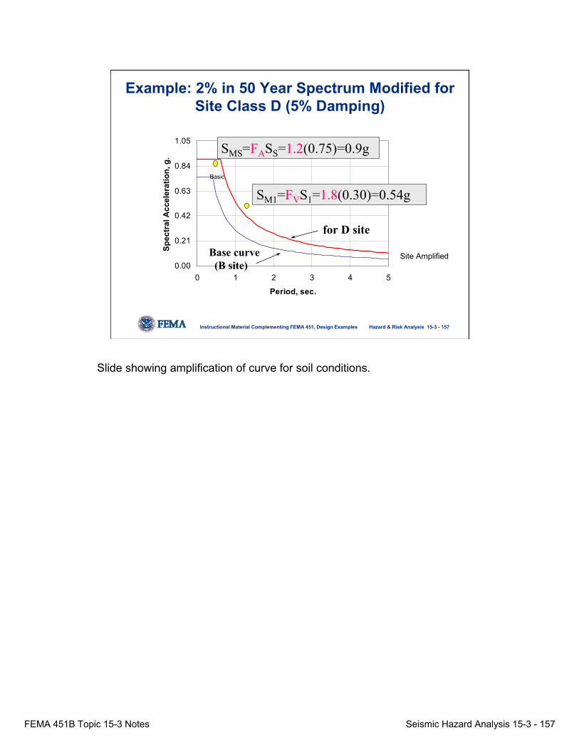
FEMA 451B Topic 15-3 Notes Seismic Hazard Analysis 15-3 - 157
Hazard & Risk Analysis 15-3 - 157Instructional Material Complementing FEMA 451, Design Examples
0.00
0.21
0.42
0.63
0.84
1.05
0 1 2 3 4 5
Period, sec.
Spec
tral
Acc
eler
atio
n, g
.
SMS=FASS=1.2(0.75)=0.9g
SM1=FVS1=1.8(0.30)=0.54gBasic
Site Amplified
Example: 2% in 50 Year Spectrum Modified for Site Class D (5% Damping)
Base curve(B site)
for D site
Slide showing amplification of curve for soil conditions.

FEMA 451B Topic 15-3 Notes Seismic Hazard Analysis 15-3 - 158
Hazard & Risk Analysis 15-3 - 158Instructional Material Complementing FEMA 451, Design Examples
IBC 2003 - General Procedure
• Adjust MCE values of Ss and S1 for local site effects:
SMS = Fa•Ss SM1 = Fv•S1
• Calculate the spectral design values SDS and SD1:
SDS = 2/3•SMS SD1 = 2/3•SM1
Note the 2/3 multiplier to reduce the motions from the MCE level.

FEMA 451B Topic 15-3 Notes Seismic Hazard Analysis 15-3 - 159
Hazard & Risk Analysis 15-3 - 159Instructional Material Complementing FEMA 451, Design Examples
IBC2003 – General Procedure
• From SDS and SMS, develop the design response spectrum
SD1
SDS
Sa=SD1/ T
1.0To
SPEC
TRA
L R
ESPO
NSE
A
CC
ELER
ATI
ON
Sa
DESIGN RESPONSE SPECTRUM
Ts
PERIOD T
Smoothed spectrum used for design. Spectrum anchored by USGS/IBC map values at short (To) and long (T = 1 sec) period.
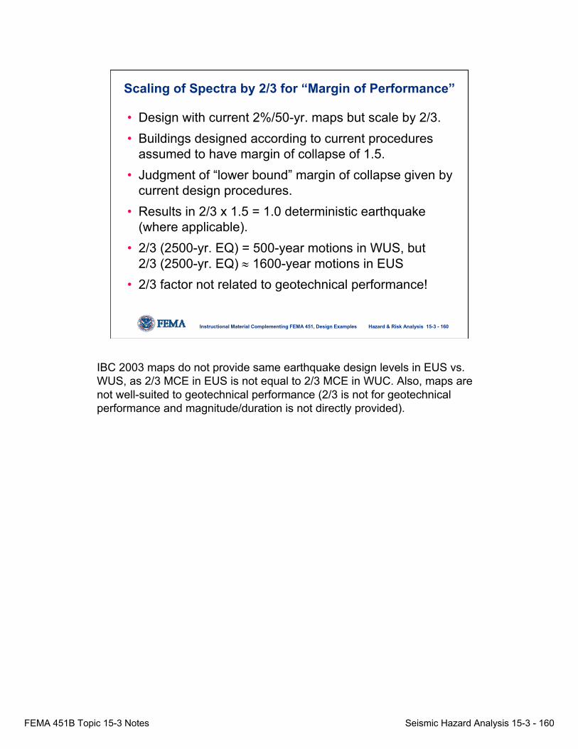
FEMA 451B Topic 15-3 Notes Seismic Hazard Analysis 15-3 - 160
Hazard & Risk Analysis 15-3 - 160Instructional Material Complementing FEMA 451, Design Examples
• Design with current 2%/50-yr. maps but scale by 2/3.• Buildings designed according to current procedures
assumed to have margin of collapse of 1.5.• Judgment of “lower bound” margin of collapse given by
current design procedures.• Results in 2/3 x 1.5 = 1.0 deterministic earthquake
(where applicable).• 2/3 (2500-yr. EQ) = 500-year motions in WUS, but
2/3 (2500-yr. EQ) ≈ 1600-year motions in EUS• 2/3 factor not related to geotechnical performance!
Scaling of Spectra by 2/3 for “Margin of Performance”
IBC 2003 maps do not provide same earthquake design levels in EUS vs. WUS, as 2/3 MCE in EUS is not equal to 2/3 MCE in WUC. Also, maps are not well-suited to geotechnical performance (2/3 is not for geotechnical performance and magnitude/duration is not directly provided).
FEMA 451B Topic 15-3 Notes Seismic Hazard Analysis 15-3 - 161
Hazard & Risk Analysis 15-3 - 161Instructional Material Complementing FEMA 451, Design Examples
Three Classes of Methods forGround Motion Estimates
• Generalized, simplified (i.e., IBC 2003)
• Site-specific, simplified (i.e., attenuation curves, site amplification factors) ⇐
• Site-specific, rigorous (time history analysis)
None.
FEMA 451B Topic 15-3 Notes Seismic Hazard Analysis 15-3 - 162
Hazard & Risk Analysis 15-3 - 162Instructional Material Complementing FEMA 451, Design Examples
Site-Specific, Simplified• Relatively simple (chart-based procedures).
• Based on probabilistic motions or deterministic scenarios.
• Can account for regional geological effects (within 2 km of surface; USGS maps assume standard depth for B-C boundary and hard rock).
• Accounts for local site (within few hundred feet of surface) effects in simplified, but more specific manner.
• Better-suited to many geotechnical analyses.
Relatively simple (chart-based procedures) are used for may preliminary and approximate analysis.

FEMA 451B Topic 15-3 Notes Seismic Hazard Analysis 15-3 - 163
Hazard & Risk Analysis 15-3 - 163Instructional Material Complementing FEMA 451, Design Examples
Site-Specific, Simplified: Comments
• Note IBC 2003 limits site-specific “benefit” (in terms of reduced design) motions to 20% for A-E sites.
• Site-specific analysis in some CEUS area less than probabilistic maps values; opposite may be true in WUS.
None.

FEMA 451B Topic 15-3 Notes Seismic Hazard Analysis 15-3 - 164
Hazard & Risk Analysis 15-3 - 164Instructional Material Complementing FEMA 451, Design Examples
Site-Specific Simplified ProceduresTypical deterministic scenario:
1. Knowing fault location and earthquake magnitude, estimate ground motion parameter (i.e, pga or spectral values) for hard rock from attenuation relationships.
2. If appropriate, correct for regional geological conditions such as deep unconsolidated sediments (Vs >700m/s and typically within 2 km of surface)
3. Modify motions for near-surface soils (Vs < 700 m/s and within few hundred of surface)*
*covered in detail in a following lecture.
None.
FEMA 451B Topic 15-3 Notes Seismic Hazard Analysis 15-3 - 165
Hazard & Risk Analysis 15-3 - 165Instructional Material Complementing FEMA 451, Design Examples
1. Estimating Motions on Hard Rock
• Typically use region-specific attenuation curve (but can use probabilistic maps also).
• Curves developed from empirical data from recorded motions in most regions.
• Curves in CEUS developed from few small EQs, plus stochastic simulations using methods developed in WUS but with CEUS geological parameters (Q, stress drop, etc.).
• Most curves provide PGA, PGV, and spectral values.
None.
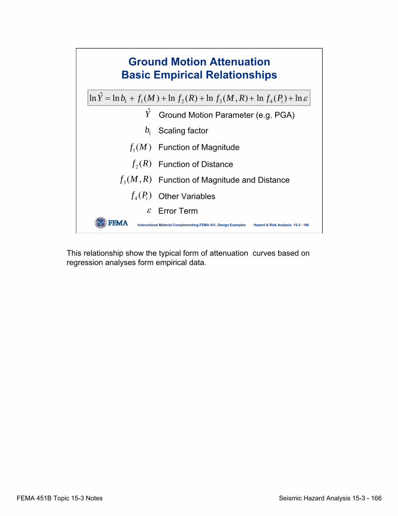
FEMA 451B Topic 15-3 Notes Seismic Hazard Analysis 15-3 - 166
Hazard & Risk Analysis 15-3 - 166Instructional Material Complementing FEMA 451, Design Examples
εln)(ln),(ln)(ln)(lnˆln 43211 +++++= iPfRMfRfMfbY
1b
)(1 Mf
)(2 Rf
),(3 RMf
)(4 iPfε
Scaling factor
Function of Magnitude
Function of Distance
Function of Magnitude and Distance
Other Variables
Error Term
Y Ground Motion Parameter (e.g. PGA)
Ground Motion AttenuationBasic Empirical Relationships
This relationship show the typical form of attenuation curves based on regression analyses form empirical data.

FEMA 451B Topic 15-3 Notes Seismic Hazard Analysis 15-3 - 167
Hazard & Risk Analysis 15-3 - 167Instructional Material Complementing FEMA 451, Design Examples
• Central and Eastern US• Subduction Zone Earthquakes• Shallow Crustal Earthquakes• Near-Source Attenuation• Extensional Tectonic Regions• Many Others• Most are for hard rock, some for “soil”
May be developed for any desired quantity(PGA, PGV, Spectral Response)
Ground Motion AttenuationRelationships for Different Conditions
A number of attenuation curves are available for specific source and site conditions.

FEMA 451B Topic 15-3 Notes Seismic Hazard Analysis 15-3 - 168
Hazard & Risk Analysis 15-3 - 168Instructional Material Complementing FEMA 451, Design Examples
Seismological Research LettersVolume 68, Number 1January/February, 1997
Ground Motion AttenuationRelationships
This slide indicates an excellent reference on recent attenuation relationships in the US.

FEMA 451B Topic 15-3 Notes Seismic Hazard Analysis 15-3 - 169
Hazard & Risk Analysis 15-3 - 169Instructional Material Complementing FEMA 451, Design Examples
Attenuation Relation for Shallow Crustal Earthquakes(Sadigh, Chang, Egan, Makdisi, and Youngs; for Rock and “Soil”)
Note that there is high variability in PGAs for various site conditions.

FEMA 451B Topic 15-3 Notes Seismic Hazard Analysis 15-3 - 170
Hazard & Risk Analysis 15-3 - 170Instructional Material Complementing FEMA 451, Design Examples
)2())exp(ln()5.8()ln( 7654321 +++++−++= ruprup rCMCCrCMCMCCy
T C1 C2 C3 C4 C5 C6 C7
PGA -0.624 1.000 0.000 -2.100 1.296 0.250 0.0000.07 0.110 1.000 0.006 -2.128 1.296 0.250 -0.0820.1 0.275 1.000 0.006 -2.148 1.296 0.250 -0.0410.2 0.153 1.000 -0.004 -2.080 1.296 0.250 0.0000.3 -0.057 1.000 -0.017 -2.028 1.296 0.250 0.0000.4 -0.298 1.000 -0.028 -1.990 1.296 0.250 0.0000.5 -0.588 1.000 -0.040 -1.945 1.296 0.250 0.0000.75 -1.208 1.000 -0.050 -1.865 1.296 0.250 0.0001 -1.705 1.000 -0.055 -1.800 1.296 0.250 0.0001.5 -2.407 1.000 -0.065 -1.725 1.296 0.250 0.0002 -2.945 1.000 -0.070 -1.670 1.296 0.250 0.0003 -3.700 1.000 -0.080 -1.610 1.296 0.250 0.0004 -4.230 1.000 -0.100 -1.570 1.296 0.250 0.000
Table for Magnitude <= 6.5
Attenuation Relation for Shallow Crustal Earthquakes(Sadigh, Chang, Egan, Makdisi, and Youngs)
Table of coefficients for use in attenuation equation.

FEMA 451B Topic 15-3 Notes Seismic Hazard Analysis 15-3 - 171
Hazard & Risk Analysis 15-3 - 171Instructional Material Complementing FEMA 451, Design Examples
0.001
0.01
0.1
1
1 10 100 1000
Distance, KM
Peak
Gro
und
Acc
eler
atio
n, G
45678
Magnitude
• typically use mean or 84th percentile (+1σ) values
Attenuation Relation for Shallow Crustal Earthquakes(for Western US on rock; from Sadigh et al., 1997 )
Attenuation of PGA vs. distance for shallow crustal earthquakes; from “Crustal Earthquakes Based on California Strong Motion Data,” by K. Sadigh, C.-Y. Chang, J.A. Egan, F. Makdisi, and R.R. Youngs, Seismological Research Letters, 68, January/February, 1997.

FEMA 451B Topic 15-3 Notes Seismic Hazard Analysis 15-3 - 172
Hazard & Risk Analysis 15-3 - 172Instructional Material Complementing FEMA 451, Design Examples
0.001
0.01
0.1
1
10
1 10 100 1000
Distance, KM
0.2
Sec.
Spe
ctra
l Acc
eler
atio
n, G
45678
0.001
0.01
0.1
1
10
1 10 100 1000
Distance, KM
1.0
Sec.
Spe
ctra
l Acc
eler
atio
n, G
45678
Magnitude Magnitude
0.2 Second Acceleration 1.0 Second Acceleration
Attenuation Relation for Shallow Crustal Earthquakes(Western US, rock conditions; Sadigh et al., 1997)
For western US on rock from “Crustal Earthquakes Based on California Strong Motion Data,” by K. Sadigh, C.-Y. Chang, J.A. Egan, F. Makdisi, and R.R. Youngs, Seismological Research Letters, 68, January/February, 1997.

FEMA 451B Topic 15-3 Notes Seismic Hazard Analysis 15-3 - 173
Hazard & Risk Analysis 15-3 - 173Instructional Material Complementing FEMA 451, Design Examples
In some regions, the presence of deep unconsolidated sediments (“soil” to geologists, “soft rock” to engineers; Vs ≈ 700 m/s) require correction of hard rock values for these conditions. Can use:
• Regional correction curve to adjust hard rock curve; or,
• A “soil” attenuation curve in Step 1 that already includes the effect of the “soil” as soil attenuation curve. In this case, the correction here for Step 2 is not required.
2. Adjustment for Regional Geology
The presence of deep unconsolidated sediments (“soil” to geologists, “soft rock” to engineers; Vs ≈ 700 m/s) require correction of hard rock values as illustrated in the following slides.

FEMA 451B Topic 15-3 Notes Seismic Hazard Analysis 15-3 - 174
Hazard & Risk Analysis 15-3 - 174Instructional Material Complementing FEMA 451, Design Examples
Shear wave velocity (ft/s)0 1000 2000 3000 4000 5000
Dep
th b
elow
gro
und
surfa
ce (f
t)
0
100
200
300
400
500
600
700
800
900
1000
1100
Soil
Soft Rock
Hard Rock
~12000 ft/s
Example: CEUS Geological Condition Requiring Adjustment:
Soil conditions such as those depicted above are common in the central and eastern US such as Memphis and Charleston.

FEMA 451B Topic 15-3 Notes Seismic Hazard Analysis 15-3 - 175
Hazard & Risk Analysis 15-3 - 175Instructional Material Complementing FEMA 451, Design Examples
EUS Hard Rock Response Spectrum(adjust with regional soil amplification curve)
Period (sec)
10-2 10-1 100 101
Spe
ctra
l Acc
eler
atio
n (g
)
10-2
10-1
100
101
Atkinson and Boore (1995) ModelMw = 7.3 R = 14.1 km
EUS Hard Rock Response Spectrum from Atkinson and Boore (1995) Model for the case where Mw = 7.3, and distance, R, = 14.1 km.

FEMA 451B Topic 15-3 Notes Seismic Hazard Analysis 15-3 - 176
Hazard & Risk Analysis 15-3 - 176Instructional Material Complementing FEMA 451, Design Examples
Regional “Soil” Amplification Factors(use to adjust hard rock curve)
Atkinson and Boore (1997)Period (sec)
10-1 100
Spec
tral A
mpl
ifica
tion
0.8
1.0
1.2
1.4
1.6
1.8
2.0
2.2
• Amplification with respect to hard rock
• Deep soil profile representative of Site Class C soil profile
The amplification curve for the deep soil profile with respect to hard rock is shown, and it can be seen that the low periods (high frequencies) will be deamplified and the high periods will be amplified. This is similar to the response expected in Memphis with about 1000 ft. of unconsolidated soil and in Charleston with 800 m of such material.
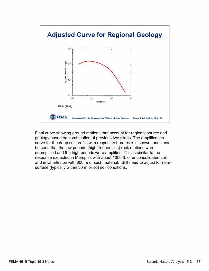
FEMA 451B Topic 15-3 Notes Seismic Hazard Analysis 15-3 - 177
Hazard & Risk Analysis 15-3 - 177Instructional Material Complementing FEMA 451, Design Examples
Adjusted Curve for Regional Geology
EPRI (1993)
Period (sec)
10-2 10-1 100 101
Spec
tral A
ccel
erat
ion
(g)
10-2
10-1
100
101
Final curve showing ground motions that account for regional source and geology based on combination of previous two slides. The amplification curve for the deep soil profile with respect to hard rock is shown, and it can be seen that the low periods (high frequencies) rock motions were deamplified and the high periods were amplified. This is similar to the response expected in Memphis with about 1000 ft. of unconsolidated soil and in Charleston with 800 m of such material. Still need to adjust for near-surface (typically within 30 m or so) soil conditions.

FEMA 451B Topic 15-3 Notes Seismic Hazard Analysis 15-3 - 178
Hazard & Risk Analysis 15-3 - 178Instructional Material Complementing FEMA 451, Design Examples
“Soil” Attenuation Relationships
Boore and Joyner (1991)
rhypo (km)
101 102 103
Sa
(cm
/s2 )
100
101
102
103
104
T = 0.2 sec
M = 8M = 7M = 6
M = 5
rhypo (km)
101 102 103
Sa
(cm
/s2 )
104
102
100
10-2
T = 1.0 sec
M = 8M = 7M = 6
M = 5
• Can use these directly where appropriate and available in lieu of two-step procedure:
Some relationships are developed for specific regions and already account for the presence of local geological conditions.

FEMA 451B Topic 15-3 Notes Seismic Hazard Analysis 15-3 - 179
Hazard & Risk Analysis 15-3 - 179Instructional Material Complementing FEMA 451, Design Examples
3. Adjustment for near-surface soil conditions (within ~30 m depth)
• pga adjustment using amplification factors
Soft soils can amplify PGAs relative to rock in many cases. Seed and Idriss (1984) and Idriss (1990). Such relationships are very approximate and should be used only when more rigorous methods are unavailable or unwarranted, such as for preliminary analysis.

FEMA 451B Topic 15-3 Notes Seismic Hazard Analysis 15-3 - 180
Hazard & Risk Analysis 15-3 - 180Instructional Material Complementing FEMA 451, Design Examples
• spectral adjustment using amplification factors
3. Adjustment for local soil conditions
Soft soils affect the shape and ordinate position of the response spectrum, as shown depicted by the red curve.
FEMA 451B Topic 15-3 Notes Seismic Hazard Analysis 15-3 - 181
Hazard & Risk Analysis 15-3 - 181Instructional Material Complementing FEMA 451, Design Examples
Three Classes of Methods forGround Motion Estimates
• Generalized, simplified (i.e., IBC 2003)
• Site-specific, simplified (i.e., attenuation curves, site amplification factors)
• Site-specific, rigorous (time history analysis) ⇐
None.
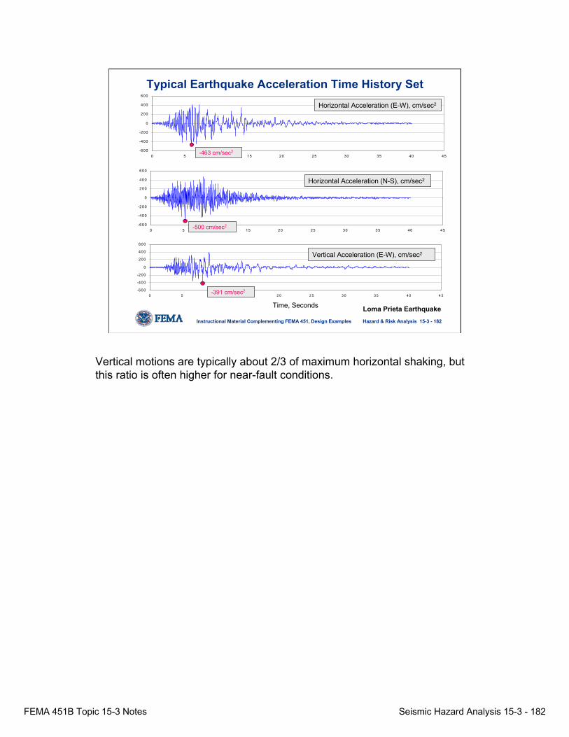
FEMA 451B Topic 15-3 Notes Seismic Hazard Analysis 15-3 - 182
Hazard & Risk Analysis 15-3 - 182Instructional Material Complementing FEMA 451, Design Examples
-600
-400
-200
0
200
400
600
0 5 10 15 20 25 30 35 40 45
-600
-400
-200
0
200
400
600
0 5 10 15 20 25 30 35 40 45
-600
-400
-200
0
200
400
600
0 5 1 0 1 5 2 0 2 5 3 0 3 5 4 0 4 5
Tim e (s e c)
Horizontal Acceleration (E-W), cm/sec2
Vertical Acceleration (E-W), cm/sec2
Horizontal Acceleration (N-S), cm/sec2
Time, Seconds Loma Prieta Earthquake
-463 cm/sec2
-500 cm/sec2
-391 cm/sec2
Typical Earthquake Acceleration Time History Set
Vertical motions are typically about 2/3 of maximum horizontal shaking, but this ratio is often higher for near-fault conditions.

FEMA 451B Topic 15-3 Notes Seismic Hazard Analysis 15-3 - 183
Hazard & Risk Analysis 15-3 - 183Instructional Material Complementing FEMA 451, Design Examples
Time History analyses• Allows best possible analysis (usually)• Increasing in usage• Time histories can be obtained from:
Databases of recorded motions such as – National and state data catalogs (NSMDS)– USGS web page – other sources (i.e., NONLIN)
By developing the motions using– modified recorded motions – synthetic motions
None.
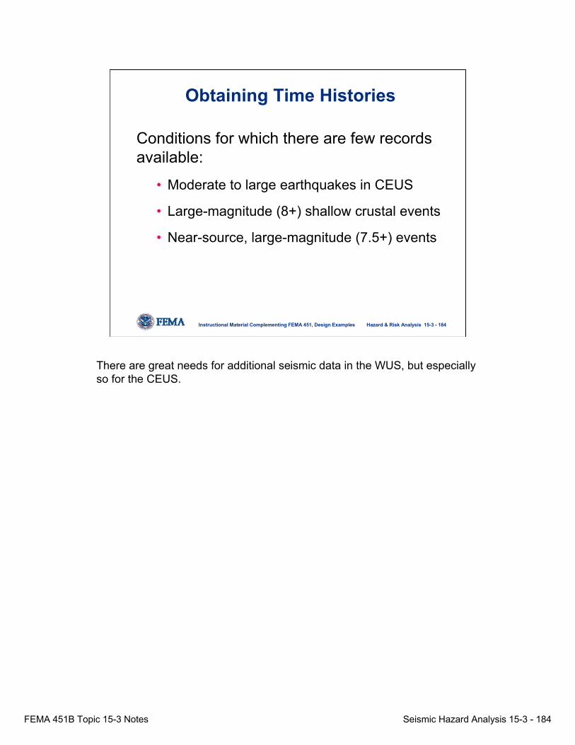
FEMA 451B Topic 15-3 Notes Seismic Hazard Analysis 15-3 - 184
Hazard & Risk Analysis 15-3 - 184Instructional Material Complementing FEMA 451, Design Examples
Obtaining Time Histories
Conditions for which there are few records available:
• Moderate to large earthquakes in CEUS
• Large-magnitude (8+) shallow crustal events
• Near-source, large-magnitude (7.5+) events
There are great needs for additional seismic data in the WUS, but especially so for the CEUS.

FEMA 451B Topic 15-3 Notes Seismic Hazard Analysis 15-3 - 185
Hazard & Risk Analysis 15-3 - 185Instructional Material Complementing FEMA 451, Design Examples
Time History Analysis• Objective: develop a set or sets of time-
histories, usually acceleration time histories, that are representative of site ground motions for the design earthquake(s)* and that are appropriate for the type of analyses planned.
• Will not be able to predict actual motions, rather interested in representing characteristics most important for design.
__________________* Discussed earlier. The design earthquake can be from deterministic or
probabilistic analysis; but, if probabilistic, the uniform hazard spectrum should probably not be used as the target spectrum. Rather, deterministic scenarios should be developed from deaggregation of the PSHA.
The design earthquake can be deterministic or probabilistic; but, if probabilistic, the uniform hazard spectrum should probably not be used as the target spectrum. Rather, deterministic scenarios should be developed from deaggregation of the PSHA.

FEMA 451B Topic 15-3 Notes Seismic Hazard Analysis 15-3 - 186
Hazard & Risk Analysis 15-3 - 186Instructional Material Complementing FEMA 451, Design Examples
Process for selecting/modifying time histories:
From: (USACE, 2000)
The table above can be used as a guide for the selection of time histories. This was adapted from the United States Army Corps of Engineers (USACE) (2000). “Time history of dynamic analysis of concrete hydraulic structures,”Engineering Circular (EC) 1110-2-6051, Department of the Army, Washington, D.C.

FEMA 451B Topic 15-3 Notes Seismic Hazard Analysis 15-3 - 187
Hazard & Risk Analysis 15-3 - 187Instructional Material Complementing FEMA 451, Design Examples
How many time histories are needed for a typical analysis?
• For linear analysis, typically 2 or 3(linear system is more influenced by frequency-domain aspects of motion)
• For non-linear analysis, typically 4 or 5(non-linear systems more influenced by time-domain aspects of record- shape and sequences of pulses, etc.)
The number of time histories to be used in an analysis, depends upon the type of analysis to be performed.
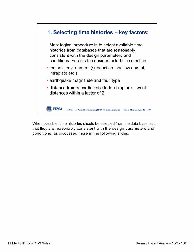
FEMA 451B Topic 15-3 Notes Seismic Hazard Analysis 15-3 - 188
Hazard & Risk Analysis 15-3 - 188Instructional Material Complementing FEMA 451, Design Examples
1. Selecting time histories – key factors:
Most logical procedure is to select available time histories from databases that are reasonably consistent with the design parameters and conditions. Factors to consider include in selection:
• tectonic environment (subduction, shallow crustal, intraplate,etc.)
• earthquake magnitude and fault type
• distance from recording site to fault rupture – want distances within a factor of 2
When possible, time histories should be selected from the data base such that they are reasonably consistent with the design parameters and conditions, as discussed more in the following slides.
FEMA 451B Topic 15-3 Notes Seismic Hazard Analysis 15-3 - 189
Hazard & Risk Analysis 15-3 - 189Instructional Material Complementing FEMA 451, Design Examples
1. Selecting time histories – key factors:
• site conditions at recording site (want similar)• response spectra of motions (want similar shape
and level to design spectra; also, want to achieve reasonable match by scaling by factor ≤ 2.0 (especially if scaling record motions to higher level)
• duration of strong shaking • if site is near-field (within about 15 km) then
acceleration record should contain strong motion pulse similar to that caused directivity, etc.
None.
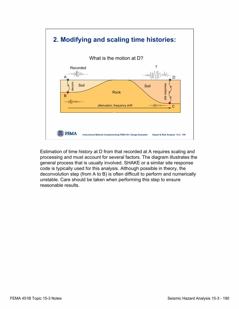
FEMA 451B Topic 15-3 Notes Seismic Hazard Analysis 15-3 - 190
Hazard & Risk Analysis 15-3 - 190Instructional Material Complementing FEMA 451, Design Examples
?
2. Modifying and scaling time histories:
What is the motion at D?
Rock
attenuation, frequency shift
Soil Soil
A
Recorded
B
C
Dde
conv
.
site
resp
onse
Estimation of time history at D from that recorded at A requires scaling and processing and must account for several factors. The diagram illustrates the general process that is usually involved. SHAKE or a similar site response code is typically used for this analysis. Although possible in theory, the deconvolution step (from A to B) is often difficult to perform and numerically unstable. Care should be taken when performing this step to ensure reasonable results.

FEMA 451B Topic 15-3 Notes Seismic Hazard Analysis 15-3 - 191
Hazard & Risk Analysis 15-3 - 191Instructional Material Complementing FEMA 451, Design Examples
2. Modifying and scaling time histories:
(a) Simple scaling – scale motions by single factor to match target spectrum;again limiting the scaling factor to 2.0.
• The required degree–of-fit to target spectrum is project-dependent, but typically want suite of candidate spectra to have average visual fit to target. More important to have conservative fit in period range of interest.
The required degree-of-fit to target spectrum is project-dependent, but typically want suite of candidate spectra to have average visual fit to target. More important to have conservative fit in period range of interest.

FEMA 451B Topic 15-3 Notes Seismic Hazard Analysis 15-3 - 192
Hazard & Risk Analysis 15-3 - 192Instructional Material Complementing FEMA 451, Design Examples
Simple Scaling to Match Design (Target) Spectrum
Real record shown (Sierra point from 1989 LPE) in plot was scaled up from 0.06g to 0.16g (target) using factor of 2.8-- too high ideally, but was deemed acceptable because of reasonable spectral match in period range of interest (∼ 1 sec.) and a lack of other recordings.
time (sec)
0 5 10 15 20 25 30 35 40
acce
lera
tion
(g)
-0.15-0.10-0.050.000.050.100.15
Period (sec)0.01 0.1 1 10
PS
A (g
)
0.0
0.1
0.2
0.3
0.4
0.5
Target design spectrum
Spectrum of scaled real record
scaled time history
Example of matching target spectrum. It can be seen that the spectral shape of the Sierra Point record matches the target reasonably well, but may not be conservative enough for certain projects, such as nuclear sites that typically require 95% of the points to be equal to higher than the target.
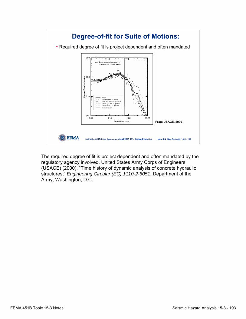
FEMA 451B Topic 15-3 Notes Seismic Hazard Analysis 15-3 - 193
Hazard & Risk Analysis 15-3 - 193Instructional Material Complementing FEMA 451, Design Examples
• Required degree of fit is project dependent and often mandated
Degree-of-fit for Suite of Motions:
From USACE, 2000
The required degree of fit is project dependent and often mandated by the regulatory agency involved. United States Army Corps of Engineers (USACE) (2000). “Time history of dynamic analysis of concrete hydraulic structures,” Engineering Circular (EC) 1110-2-6051, Department of the Army, Washington, D.C.
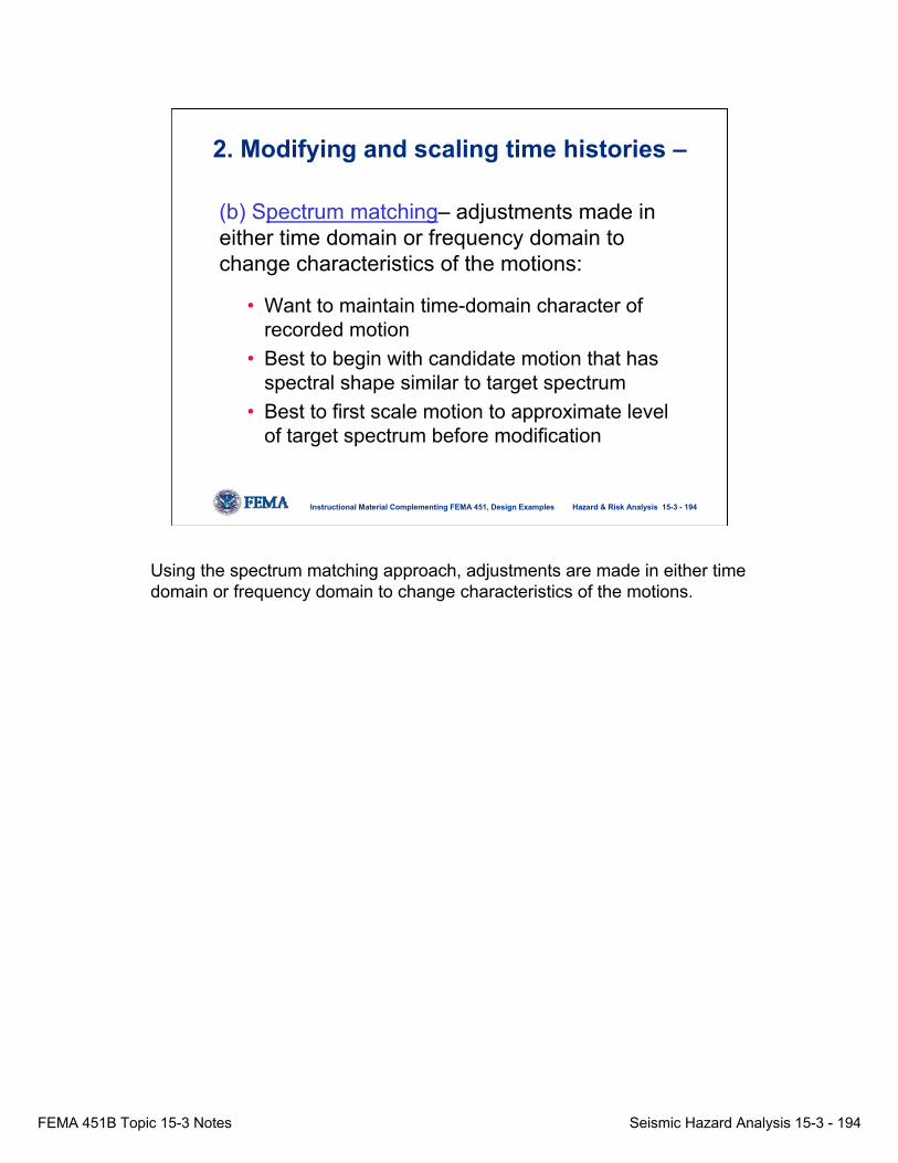
FEMA 451B Topic 15-3 Notes Seismic Hazard Analysis 15-3 - 194
Hazard & Risk Analysis 15-3 - 194Instructional Material Complementing FEMA 451, Design Examples
2. Modifying and scaling time histories –
(b) Spectrum matching– adjustments made in either time domain or frequency domain to change characteristics of the motions:
• Want to maintain time-domain character of recorded motion
• Best to begin with candidate motion that has spectral shape similar to target spectrum
• Best to first scale motion to approximate level of target spectrum before modification
Using the spectrum matching approach, adjustments are made in either time domain or frequency domain to change characteristics of the motions.

FEMA 451B Topic 15-3 Notes Seismic Hazard Analysis 15-3 - 195
Hazard & Risk Analysis 15-3 - 195Instructional Material Complementing FEMA 451, Design Examples
Spectrum Matching Methods(i) Time-Domain Approach: (Lilhanand and Tseng, 1988; Abrahamson, 1992).
• Matching accomplished by adding (or subtracting) finite-duration wavelets to (or from) the initial time-history.
• Normally provides a close fit to the target. Best to being with candidate motion has spectral shape similar to target spectrum.
• Best to first scale motion to approximate level of target spectrum before modification.
With the time-domain approach, matching is accomplished by adding (or subtracting) finite-duration wavelets to (or from) the initial time-history.

FEMA 451B Topic 15-3 Notes Seismic Hazard Analysis 15-3 - 196
Hazard & Risk Analysis 15-3 - 196Instructional Material Complementing FEMA 451, Design Examples
Spectrum Matching Methods
(ii) Frequency-Domain Approach: (Gasparini and Vanmarcke 1976; Silva and Lee 1987; Bolt and Gregor 1993).
• Adjusts only the Fourier amplitudes while the Fourier phases are kept unchanged.
• Procedure equivalent to adding or subtracting sinusoids (with the Fourier phases of the initial time-history) in the time domain.
• Does not always provide as close a fit as time-domain approach.
The frequency-domain approach adjusts only the Fourier amplitudes, while the Fourier phases are kept unchanged.
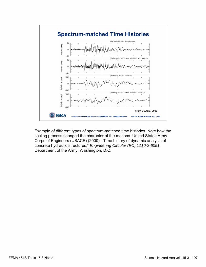
FEMA 451B Topic 15-3 Notes Seismic Hazard Analysis 15-3 - 197
Hazard & Risk Analysis 15-3 - 197Instructional Material Complementing FEMA 451, Design Examples
Spectrum-matched Time Histories
From USACE, 2000
Example of different types of spectrum-matched time histories. Note how the scaling process changed the character of the motions. United States Army Corps of Engineers (USACE) (2000). “Time history of dynamic analysis of concrete hydraulic structures,” Engineering Circular (EC) 1110-2-6051, Department of the Army, Washington, D.C.
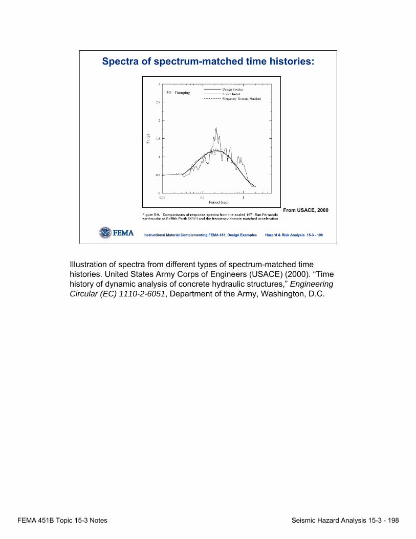
FEMA 451B Topic 15-3 Notes Seismic Hazard Analysis 15-3 - 198
Hazard & Risk Analysis 15-3 - 198Instructional Material Complementing FEMA 451, Design Examples
Spectra of spectrum-matched time histories:
From USACE, 2000
Illustration of spectra from different types of spectrum-matched time histories. United States Army Corps of Engineers (USACE) (2000). “Time history of dynamic analysis of concrete hydraulic structures,” Engineering Circular (EC) 1110-2-6051, Department of the Army, Washington, D.C.
FEMA 451B Topic 15-3 Notes Seismic Hazard Analysis 15-3 - 199
Hazard & Risk Analysis 15-3 - 199Instructional Material Complementing FEMA 451, Design Examples
Other corrections…
• Ensure records are instrument and base-line corrected, etc.
It is important to ensure that records are instrument- and base-line corrected, especially if displacements are to be calculated.

FEMA 451B Topic 15-3 Notes Seismic Hazard Analysis 15-3 - 200
Hazard & Risk Analysis 15-3 - 200Instructional Material Complementing FEMA 451, Design Examples
3. Modification for local site conditions
• Dynamic site response analysis is best approach (discussed in following lecture).
None.

FEMA 451B Topic 15-3 Notes Seismic Hazard Analysis 15-3 - 201
Hazard & Risk Analysis 15-3 - 201Instructional Material Complementing FEMA 451, Design Examples
Real vs. Synthetic Time Histories
• What is considered a “real”record? (i.e., how much modification is allowed?)
• Un-scaled record motion vs. scaled recorded motion vs. synthetic.
• Synthetic motions developed using Fourier phase spectra from real earthquake probably “real” in most important ways.
The distinction between real vs. synthetic motions is not always clear– that is, a scaled real motions may be less representative of a real earthquake motions than a carefully generated synthetic motions developed using Fourier phase spectra from a real earthquake.
FEMA 451B Topic 15-3 Notes Seismic Hazard Analysis 15-3 - 202
Hazard & Risk Analysis 15-3 - 202Instructional Material Complementing FEMA 451, Design Examples
Synthetic Time Histories – Pros and Cons
• One main concern: Is true character of real motion present?
• One main advantage: Can develop motions to match regional and site conditions (i.e., motion recorded on outcrops actually have surface wave energy included but we commonly input this to base).
– there are many data gaps in database of motions (no strong motions for CEUS)
– certainly better to have reasonable region-specific synthetic motion than inappropriate real motion
None.
FEMA 451B Topic 15-3 Notes Seismic Hazard Analysis 15-3 - 203
Hazard & Risk Analysis 15-3 - 203Instructional Material Complementing FEMA 451, Design Examples
Developing Synthetic Motions
• Process should be performed by expert, typically seismologist.
• Seismologists typically develop a suite of time histories for hard rock or B-C (soft rock) boundary.
• Geotechnical engineers typically generate top-of-profile motions using site responseanalysis.
Seismologists typically develop a suite of time histories for hard rock or B-C (soft rock) boundary and geotechnical engineers typically modify this motion based on the soil profile (less than 30 m typically).
FEMA 451B Topic 15-3 Notes Seismic Hazard Analysis 15-3 - 204
Hazard & Risk Analysis 15-3 - 204Instructional Material Complementing FEMA 451, Design Examples
The computational model for generating synthetic seismograms consists of:
• The seismic source process;
• The process of seismic wave propagation from the source region to the design site; and
• Shallow site response (site response is discussed later).
Synthetic Ground Motion Development
None.
FEMA 451B Topic 15-3 Notes Seismic Hazard Analysis 15-3 - 205
Hazard & Risk Analysis 15-3 - 205Instructional Material Complementing FEMA 451, Design Examples
Source Parameters Required• Rupture velocity, rupture initiation point, and slip-
time functions over the ruptured area are the primary source parameters needed.
Propagation (Path) Parameters Required• Average propagation usually developed with
Green’s functions -- requires knowledge of the crustal parameters such as the P and S-wave velocities, density, and damping factor (or seismic Q factor, where Q = 0.5/damping ratio).
Synthetic Ground Motion Development
None.

FEMA 451B Topic 15-3 Notes Seismic Hazard Analysis 15-3 - 206
Hazard & Risk Analysis 15-3 - 206Instructional Material Complementing FEMA 451, Design Examples
• To model complexity of seismogram, randomness (stochastic model) is often introduced, either in the source process or in the wave propagation.
– very erratic, irregular high-frequency waves from rupture process usually characterized as a “stochastic” process that must be modeled with randomness
– deterministic process often used for low-frequency portion of motion
• Hybrid models combine deterministic with random process.
Synthetic Ground Motion Generation
To model complexity of a seismogram, randomness (stochastic model) is often introduced, either in the source process or in the wave propagation. Usually, the high frequency motions (> 2 or 3 Hz) are modeled stochastically and the low frequency motions are modeled deterministically.

FEMA 451B Topic 15-3 Notes Seismic Hazard Analysis 15-3 - 207
Hazard & Risk Analysis 15-3 - 207Instructional Material Complementing FEMA 451, Design Examples
• With fault slip model and Green’s functions, ground motions are computed using the representation theorem (deconvolution process); see Aki and Richards 1980; Hartzell, Frazier, and Brune 1978.
• Simulation procedure simply sums a suite of Green’s functions lagged in time (delay caused by the rupture propagation plus the time needed for the seismic waves to travel from the corresponding point source to the site).
⇒ Green’s Function is heart of the process.
Synthetic Ground Motion Generation
The Green’s function that predicts the response at one point in the earth given an action at another point is one of the most important parameters in predicting ground motions. This function contains the effects of the “path”(i.e., geology between site and source).

FEMA 451B Topic 15-3 Notes Seismic Hazard Analysis 15-3 - 208
Hazard & Risk Analysis 15-3 - 208Instructional Material Complementing FEMA 451, Design Examples
Synthetic Ground Motion Methods
(1) Boore (1983): developed Band-Limited-White-Noise model for stochastic simulation of high-frequency ground motions.
• This simulation procedure does not use stochastic slip model.
• Procedure generates random white noise, multiplies it by a window function appropriate for the expected source duration, and then filters the windowed white noise to obtain a time-history having a band-limited Fourier amplitude spectrum specified by the ω2-source Brune (1970) model.
• Incorporates wave propagation effects of a homogeneous crust with 1/R geometrical attenuation.
None.

FEMA 451B Topic 15-3 Notes Seismic Hazard Analysis 15-3 - 209
Hazard & Risk Analysis 15-3 - 209Instructional Material Complementing FEMA 451, Design Examples
Boore (1983) – Illustration of Concept*:
*Figure adapted from Kramer (1996)
Boore (1983):
Example of the time-domain generation of a synthetic time history. The slide depicts this four-step process.
FEMA 451B Topic 15-3 Notes Seismic Hazard Analysis 15-3 - 210
Hazard & Risk Analysis 15-3 - 210Instructional Material Complementing FEMA 451, Design Examples
(2) Silva and Lee (1987): method uses formulation for the Fourier amplitude spectrum similar to Boore, but the phase spectrum from a natural time-history to generate the synthetic time-history.
(3) Publicly available computer codes: Some public domain simulation codes are: RASCAL (Silva and Lee 1987) and SMSIM (Boore 1996).
⇒ The above methods (1 through 3) are well-established.
Synthetic Ground Motion Methods
An exampled using RASCAL will be presented in the following slides.

FEMA 451B Topic 15-3 Notes Seismic Hazard Analysis 15-3 - 211
Hazard & Risk Analysis 15-3 - 211Instructional Material Complementing FEMA 451, Design Examples
Example: Synthetic Motion development with RASCALa) Pseudo Spectral Acceleration for 5% oscillator damping
Period (sec)
0.01 0.1 1 10
PSA
(g)
0.00
0.05
0.10
0.15
0.20
0.25
0.30
0.35
0.40
synthetic motion (from RASCAL)SRS target spectrum
b) Synthetic motion
time (sec)
0 5 10 15 20 25 30 35 40
acce
lera
tion
(g)
-0.15
-0.10
-0.05
0.00
0.05
0.10
0.15
Example of synthetic motion development using RASCAL computer code. The RASCAL code is used to match “target” spectrum at many points. Again, depending upon the project, the closeness of the match is often specified. Nuclear power plant type projects typically require at least 95% of the points equal or exceed the target.

FEMA 451B Topic 15-3 Notes Seismic Hazard Analysis 15-3 - 212
Hazard & Risk Analysis 15-3 - 212Instructional Material Complementing FEMA 451, Design Examples
Source Modeling for Synthetic Motions1) Point source models (i.e., Brune source spectrum):
• Simple model where the source is represented by a point.• Assumes “stationary” signal; provides average component.• Need Magnitude, stress drop Δσ, density, crust modulus.
2) Finite fault models – modeling the actual rupture:• Fault is divided into segments and each segment ruptures
after another simulating energy release.• Energy radiation from each segment is modeled using
Green’s Function.• Motion from all segments added up to generate motion at
a point from the fault.• It models directivity, radiation, and non-stationarity.
Point source models are simpler to use and more common; finite fault models are for advanced analyses.
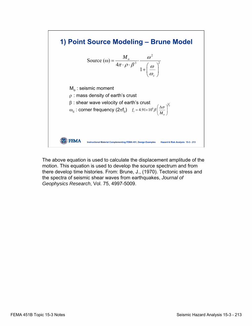
FEMA 451B Topic 15-3 Notes Seismic Hazard Analysis 15-3 - 213
Hazard & Risk Analysis 15-3 - 213Instructional Material Complementing FEMA 451, Design Examples
13
64.91 10co
fM
σβ
⎛ ⎞Δ= × ⎜ ⎟
⎝ ⎠
1) Point Source Modeling – Brune Model
Mo : seismic momentρ : mass density of earth’s crustβ : shear wave velocity of earth’s crustωc : corner frequency (2πfc)
2
23Source (ω)4
1
o
c
M ωπ ρ β ω
ω
= ⋅⋅ ⋅ ⎛ ⎞
+ ⎜ ⎟⎝ ⎠
The above equation is used to calculate the displacement amplitude of the motion. This equation is used to develop the source spectrum and from there develop time histories. From: Brune, J., (1970). Tectonic stress and the spectra of seismic shear waves from earthquakes, Journal of Geophysics Research, Vol. 75, 4997-5009.

FEMA 451B Topic 15-3 Notes Seismic Hazard Analysis 15-3 - 214
Hazard & Risk Analysis 15-3 - 214Instructional Material Complementing FEMA 451, Design Examples
Modeling Source – Brune Model
• Source spectrum for different magnitude earthquakes• Corner frequency (ωc) decreases for larger magnitudes (duration α
1/ωc)
frequency (Hz)
0.001 0.01 0.1 1 10 100
acce
lera
tion
ampl
itude
M = 8
M = 7
M = 6
M = 5
2
2341
o
c
M ωπ ρ β ω
ω
⋅⋅ ⋅ ⎛ ⎞
+ ⎜ ⎟⎝ ⎠
The Brune model is a basic source modeling scheme commonly used for many applications. This assumes an ideal, symmetrical earthquake source per se, and is much simpler than finite fault modeling. The inaccuracy of this approach is minimized with distance from the source. From: Brune, J., (1970). Tectonic stress and the spectra of seismic shear waves from earthquakes, Journal of Geophysics Research, Vol. 75, 4997-5009.

FEMA 451B Topic 15-3 Notes Seismic Hazard Analysis 15-3 - 215
Hazard & Risk Analysis 15-3 - 215Instructional Material Complementing FEMA 451, Design Examples
Modeling Path Effects
r : distance to the sourcef : frequencyβ : shear wave velocity of earth’s crustQ : quality factor (1/2D, D = damping ratio)
Q = 200 f0.2 – Western USQ = 680 f0.34 – Eastern US
( )1Path (ω)f r
Q fer
πβ−
⋅ ⋅⋅= ⋅
One the source spectrum is established, the motions are modified for attenuation through the earth’s crust. The motions are attenuated as a function of frequency.

FEMA 451B Topic 15-3 Notes Seismic Hazard Analysis 15-3 - 216
Hazard & Risk Analysis 15-3 - 216Instructional Material Complementing FEMA 451, Design Examples
Modeling Path Effects
frequency (Hz)
0.001 0.01 0.1 1 10 100
path
effe
ct
Eastern USWestern US
r = 50 km
r = 100 km
( )1f r
Q fer
πβ−
⋅ ⋅⋅⋅
• Frequency dependent attenuation• Smaller attenuation for Eastern US
Effects of different crustal conditions (EUS vs. WUS. ) and path effects. Use this spectrum to multiply the Brune source spectrum to establish the spectrum for a particular distance from the assumed point source. We can superimpose easily in the frequency domain and thus we multiply spectra together– more efficient and elegant that trying to do this in the time domain. Thus we combine all of the effects in the frequency domain to establish a final spectrum and from there we establish a time history to match the spectrum.

FEMA 451B Topic 15-3 Notes Seismic Hazard Analysis 15-3 - 217
Hazard & Risk Analysis 15-3 - 217Instructional Material Complementing FEMA 451, Design Examples
Combined Source and Path Effects
frequency (Hz)
0.001 0.01 0.1 1 10 100
acce
lera
tion
ampl
itude
Eastern USWestern US
r = 100 km
r = 50 km
• Wider band spectrum for Eastern US• Larger high frequency components for Eastern US even at large distances
This spectrum represents the combined effect both the source and path effects. This spectrum is used as the “target” spectrum to generate the time histories for this particular location. If local site effects are to be included, then consider this using site response analysis. Note the higher motions in the high-frequency range in the EUS due to the higher Q factor (stiffer rock, lower anelastic attenuation).

FEMA 451B Topic 15-3 Notes Seismic Hazard Analysis 15-3 - 218
Hazard & Risk Analysis 15-3 - 218Instructional Material Complementing FEMA 451, Design Examples
Total far-field S displacement is constructed by summation of displacement pulses for a large number of sub-faults, randomlydistributed on the fault plane.
• Approach taken is similar to that described originally by Zeng et al., Geophysical Research Letters, 1994.
• Can model some near-field effects, provides 3 components
Important Input Parameters:
1) Total Seismic Moment2) Fault dimensions3) Maximum and minimum (circular) sub-fault radii4) Sub-fault stress drop (not necessarily the static stress drop)5) Rupture velocity (spatially constant, etc.)
2) Finite Fault Model
The finite fault model is an advanced modeling technique that should be used only for the case where a reasonable amount of information is known about the relevant fault mechanisms. Otherwise, the added sophistication is unwarranted.

FEMA 451B Topic 15-3 Notes Seismic Hazard Analysis 15-3 - 219
Hazard & Risk Analysis 15-3 - 219Instructional Material Complementing FEMA 451, Design Examples
To Receiver
Sub-fault far-field displacementpulse is radiated when therupture front reaches thecenter of the sub-fault.
The area under the radiatedpulse depends upon theSub-fault moment, which inturn depends upon the radius(random) and the stress drop(constant).
The sub-faults are allowedto overlap spatially. Superpositionof the radiated pulses from the sub-faultsmodels the spatial and temporal variabilityof fault slip velocity.
Expanding Rupture Front
Fault Plane
Sub-fault
Figure above adapted from Martin Chapman, Virginia Tech department of Geological Sciences. The sub-faults are allowed to overlap spatially. Superposition of the radiated pulses from the sub-faults models the spatial and temporal variability of fault slip velocity.
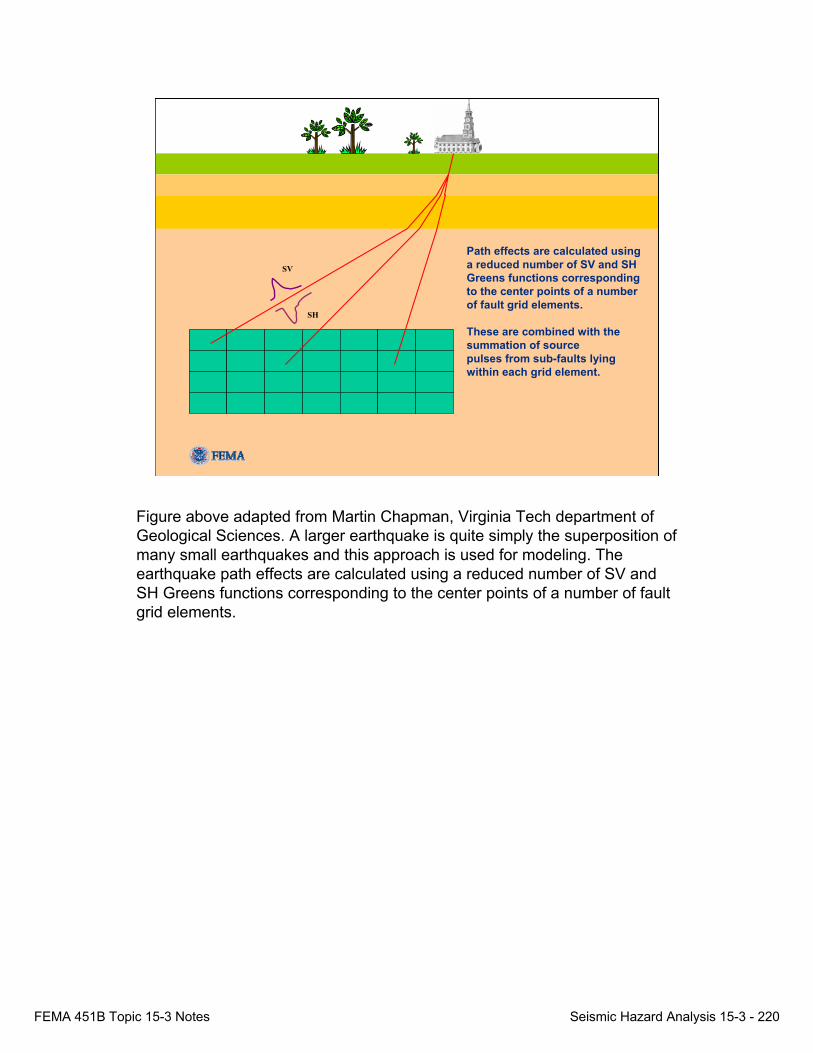
FEMA 451B Topic 15-3 Notes Seismic Hazard Analysis 15-3 - 220
Hazard & Risk Analysis 15-3 - 220Instructional Material Complementing FEMA 451, Design Examples
SV
SH
Path effects are calculated using a reduced number of SV and SH Greens functions corresponding to the center points of a number of fault grid elements.
These are combined with the summation of sourcepulses from sub-faults lying within each grid element.
Figure above adapted from Martin Chapman, Virginia Tech department of Geological Sciences. A larger earthquake is quite simply the superposition of many small earthquakes and this approach is used for modeling. The earthquake path effects are calculated using a reduced number of SV and SH Greens functions corresponding to the center points of a number of fault grid elements.

FEMA 451B Topic 15-3 Notes Seismic Hazard Analysis 15-3 - 221
Hazard & Risk Analysis 15-3 - 221Instructional Material Complementing FEMA 451, Design Examples
)()()()( fPathfPathfSourcefA seds
basesss =
).exp()exp( fkfkSourceA seds
seds
bases
basesss ππ −Φ−Φ=
).exp()/(1
)2(2
2fk
fffCA sed
sseds
cs ππ
−Φ+
=
,)2( 2 επ
π+−= fkb
fALn s
s
.)2( 2 επ
π+−= fkb
f
ALn p
sp
.()/( ) επ +−−= fkkbAALn pssps
.)(1
faGbYLn jn
jj
i π−= ∑=
s
s
p
Figure above adapted from Martin Chapman, Virginia Tech department of Geological Sciences. The Green’s function that predicts the response at one point in the earth given an action at another point is one of the most important parameters in predicting ground motions. This function contains the effects of the “path” (i.e., geology between site and source).

FEMA 451B Topic 15-3 Notes Seismic Hazard Analysis 15-3 - 222
Hazard & Risk Analysis 15-3 - 222Instructional Material Complementing FEMA 451, Design Examples
Modeling Considerations – CEUS
• Recurrence rates lower and uncertainties in source mechanisms, locations in CEUS.
• Stronger crustal structure in CEUS, therefore less attenuation.
• Stress drop?
• Too few strong motion recordings.
Modeling in the CEUS faces a number of challenges, mostly related to a lack of seismological data. A number of good references are available on this specialized area of engineering seismology such as: Boore, D. M., Joyner, W. B., and Fumal, T. E. 1997. “Equations for Estimating Horizontal Response Spectra and Peak Acceleration from Western North American Earthquakes: A Summary of Recent Work,” Seismological Research Letters, Vol 68, No. 1, pp 128-153.