seismic thickness estimation: three approaches, pros and cons gregory a. partyka bp
TRANSCRIPT

Seismic Thickness Estimation: Three Approaches, Pros and Cons
Gregory A. Partyka
bp

Outline
• IntroductionIntroduction
• Three Approaches
• Examples
• Pros and Cons
Outline
• IntroductionIntroduction
• Three Approaches
• Examples
• Pros and Cons

Blocky Wedge Model
366
400
Tra
vel T
ime
(m
s)
432
466
REFLECTIVITY
Temporal Thickness (ms)
0 5040302010

Blocky Wedge Model
366
400
Tra
vel T
ime
(m
s)
432
466
Temporal Thickness (ms)
REFLECTIVITY
BANDLIMITED REFLECTIVITY (8-10-40-50hz)
+0.025
-0.025
Amplitude
366
400
Tra
vel T
ime
(m
s)
432
466
Temporal Thickness (ms)
0 5040302010
0 5040302010

Blocky Wedge Model
366
400
Tra
vel T
ime
(m
s)
432
466
Temporal Thickness (ms)
REFLECTIVITY
BANDLIMITED REFLECTIVITY (8-10-40-50hz)
+0.025
-0.025
Amplitude
366
400
Tra
vel T
ime
(m
s)
432
466
Temporal Thickness (ms)
0 5040302010
0 5040302010

Outline
• Introduction
• Three ApproachesThree Approaches
• Examples
• Pros and Cons

Three Approaches to Thickness Estimation
1. Conventional• peak-trough time separation• amplitude
2. Spectral Decomposition• 1st dominant frequency and amplitude
3. Spectral Decomposition• discrete frequency components

Three Approaches to Thickness Estimation
1.1. ConventionalConventional• peak-trough time separationpeak-trough time separation• amplitudeamplitude
2. Spectral Decomposition• 1st dominant frequency and amplitude
3. Spectral Decomposition• discrete frequency components

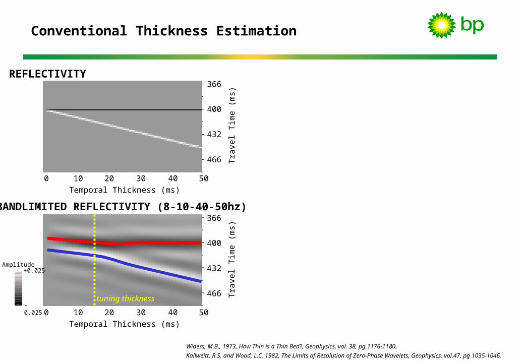
Conventional Thickness Estimation
366
400
Tra
vel T
ime
(m
s)
432
466
Temporal Thickness (ms)
REFLECTIVITY
BANDLIMITED REFLECTIVITY (8-10-40-50hz)
+0.025
-0.025
Amplitude
366
400
Tra
vel T
ime
(m
s)
432
466
Temporal Thickness (ms)
0 5040302010
0 5040302010
Conventional Thickness Estimation
366
400
Tra
vel T
ime
(m
s)
432
466
Temporal Thickness (ms)
REFLECTIVITY
BANDLIMITED REFLECTIVITY (8-10-40-50hz)
+0.025
-0.025
Amplitude
366
400
Tra
vel T
ime
(m
s)
432
466
Temporal Thickness (ms)
0 5040302010
0 5040302010
tuning thickness
Widess, M.B., 1973, How Thin is a Thin Bed?, Geophysics, vol. 38, pg 1176-1180.
Kallweitt, R.S. and Wood, L.C, 1982, The Limits of Resolution of Zero-Phase Wavelets, Geophysics, vol.47, pg 1035-1046.

-0.0250
Conventional Thickness Estimation
366
400
Tra
vel T
ime
(m
s)
432
466
Temporal Thickness (ms)
REFLECTIVITY
BANDLIMITED REFLECTIVITY (8-10-40-50hz)
+0.025
-0.025
Amplitude
366
400
Tra
vel T
ime
(m
s)
432
466
Temporal Thickness (ms)
0 5040302010
0 5040302010
0.00
5.00
10.00
15.00
20.00
25.00
30.00
35.00
40.00
45.00
50.00
0 5 10 15 20 25 30 35 40 45 50
-0.02500
-0.02000
-0.01500
-0.01000
-0.00500
0.00000
Temporal Thickness (ms)
0 5040302010
50
40
Pe
ak-
Tro
ug
h T
ime
Se
pa
ratio
n (
ms)
30
20
10
0
-0.0000
La
rge
st N
eg
ativ
e A
mp
litu
de-0.0050
-0.0100
-0.0150
45
35
25
15
5
-0.0200
tuning thickness
tuning thickness =1
1.4 * frequencyupper
tuning thickness
Widess, M.B., 1973, How Thin is a Thin Bed?, Geophysics, vol. 38, pg 1176-1180.
Kallweitt, R.S. and Wood, L.C, 1982, The Limits of Resolution of Zero-Phase Wavelets, Geophysics, vol.47, pg 1035-1046.

Three Approaches to Thickness Estimation
1. Conventional• peak-trough time separation• amplitude
2.2. Spectral DecompositionSpectral Decomposition• 11stst dominant frequency and amplitude dominant frequency and amplitude
3. Spectral Decomposition• discrete frequency components

Spectral Decomposition
• uses the discrete Fourier transform to:– quantify thin-bed interference, and– detect subtle discontinuities.

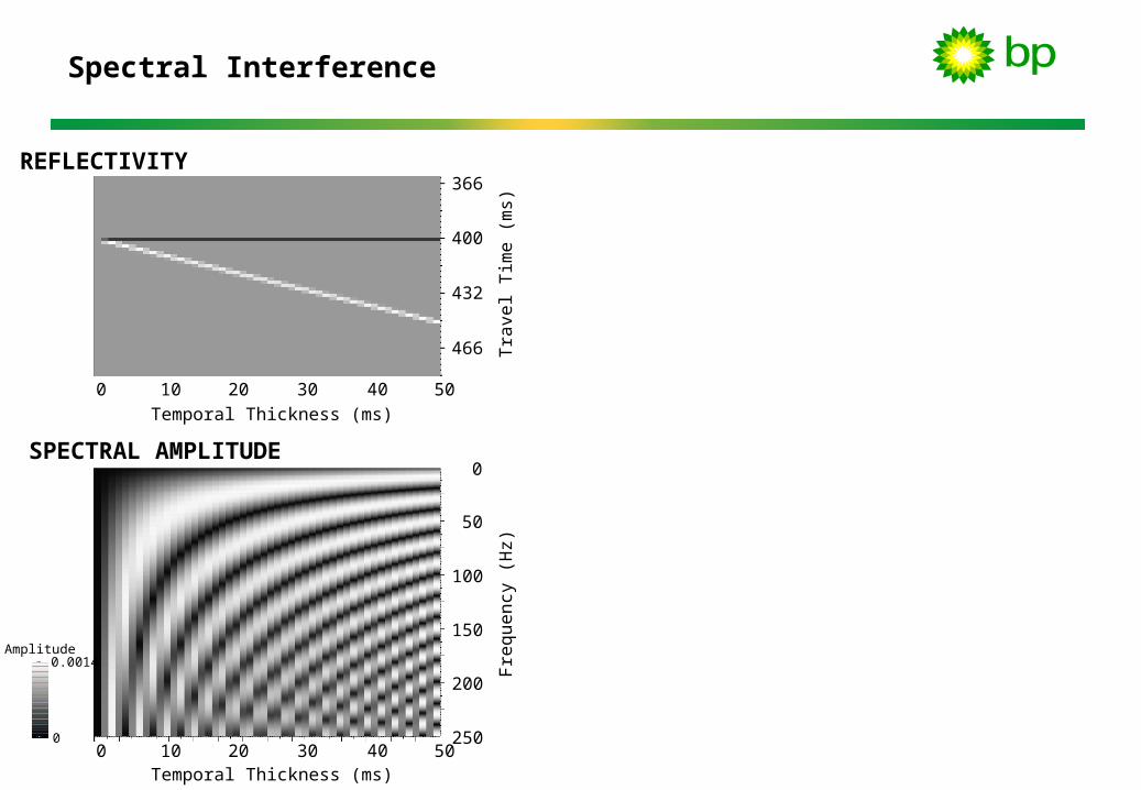
Spectral Interference
Source WaveletAmplitude Spectrum
Thin Bed ReflectionAmplitude Spectrum
Thin BedReflection
ReflectedWavelets
SourceWavelet
Thin Bed
ReflectivityAcousticImpedance
Temporal Thickness
FourierTransform
FourierTransform
Amplitude Amplitude
Fre
quen
cy
Fre
quen
cy
Temporal Thickness1
• The spectral interference pattern is imposed by the distribution of acoustic properties within the short analysis window.
Paryka, Gridley and Lopez, The Leading Edge, vol 18, no 3, 1999

Blocky Wedge Model
366
400
Tra
vel T
ime
(m
s)
432
466
REFLECTIVITY
Temporal Thickness (ms)
0 5040302010
0 5040302010
0 5040302010
Spectral Interference
366
400
Tra
vel T
ime
(m
s)
432
466
50
150
Fre
qu
en
cy (
Hz)
100
200
0
250
Temporal Thickness (ms)
REFLECTIVITY
SPECTRAL AMPLITUDE
0.0014
0
Amplitude
Temporal Thickness (ms)

0 5040302010
0 5040302010
Spectral Interference and Frequency
366
400
Tra
vel T
ime
(m
s)
432
466
50
150
Fre
qu
en
cy (
Hz)
100
200
0
250
Temporal Thickness (ms)
REFLECTIVITY
SPECTRAL AMPLITUDE
0.0014
0
Amplitude
Temporal Thickness (ms)
The temporal thickness of the wedge (t), determines the period of notching in the amplitude spectrum (Pf) with respect to frequency.
Temporal Thickness1
Temporal Thickness
Pf = 1 / t

0 5040302010
0 5040302010
Spectral Interference and Thickness
366
400
Tra
vel T
ime
(m
s)
432
466
50
150
Fre
qu
en
cy (
Hz)
100
200
0
250
Temporal Thickness (ms)
REFLECTIVITY
SPECTRAL AMPLITUDE
0.0014
0
Amplitude
Temporal Thickness (ms)
The value of the frequency component (f), determines the period of notching in the amplitude spectrum (Pt) with respect to bed thickness.
Frequency1 Pt = 1 / f

0 5040302010
0 5040302010
Spectral Interference
366
400
Tra
vel T
ime
(m
s)
432
466
50
150
Fre
qu
en
cy (
Hz)
100
200
0
250
Temporal Thickness (ms)
REFLECTIVITY
SPECTRAL AMPLITUDE
0.0014
0
Amplitude
Temporal Thickness (ms)
0 5040302010
0 5040302010
Bandwidth8-10-40-50
366
400
Tra
vel T
ime
(m
s)
432
466
BANDLIMITED REFLECTIVITY (8-10-40-50hz)
BANDLIMITED SPECTRAL AMPLITUDE
0.0014
0
Amplitude
50
150
Fre
qu
en
cy (
Hz)
100
200
0
250
Temporal Thickness (ms)
Temporal Thickness (ms)
+0.025
-0.025
Amplitude

Spectral Interference
Bandwidth8-10-40-50
0 5040302010
0 5040302010
366
400
Tra
vel T
ime
(m
s)
432
466
BANDLIMITED REFLECTIVITY (8-10-40-50hz)
BANDLIMITED SPECTRAL AMPLITUDE
0.0014
0
Amplitude
25
75
Fre
qu
en
cy (
Hz)
50
100
0
125
Temporal Thickness (ms)
Temporal Thickness (ms)
+0.025
-0.025
Amplitude

Thickness via 1st Dominant Frequency and Amplitude
Bandwidth8-10-40-50
0 5040302010
0 5040302010
366
400
Tra
vel T
ime
(m
s)
432
466
BANDLIMITED REFLECTIVITY (8-10-40-50hz)
BANDLIMITED SPECTRAL AMPLITUDE
0.0014
0
Amplitude
25
75
Fre
qu
en
cy (
Hz)
50
100
0
125
Temporal Thickness (ms)
Temporal Thickness (ms)
+0.025
-0.025
Amplitude
1st DominantFrequency

Frequencyupper and Frequency1st-dominant
= tuning thickness =1
1.4 * frequencyupper
1
2 * frequency1st-dominant

Thickness via 1st Dominant Frequency and Amplitude
1st DominantFrequency
Bandwidth8-10-40-50
0 5040302010
0 5040302010
366
400
Tra
vel T
ime
(m
s)
432
466
BANDLIMITED REFLECTIVITY (8-10-40-50hz)
BANDLIMITED SPECTRAL AMPLITUDE
0.0014
0
Amplitude
25
75
Fre
qu
en
cy (
Hz)
50
100
0
125
Temporal Thickness (ms)
Temporal Thickness (ms)
0.0000
0.0005
0.0010
0.0015
0.0020
0.0025
0
5
10
15
20
25
30
35
40
Temporal Thickness (ms)
0 5040302010
0.0014
0.0012
1st D
om
ina
nt
Am
plit
ud
e
0.0008
0.0006
0.0002
0.0000
40
35
1st D
om
ina
nt
Fre
qu
en
cy30
25
20
10
5
0
15
+0.025
-0.025
Amplitude
tuning thickness tuning thickness
tuning thickness =1
2 * frequency
0.014sec =1
2 * 36hz
1st-dominant

Three Approaches to Thickness Estimation
1. Conventional• peak-trough time separation• amplitude
2. Spectral Decomposition• 1st dominant frequency and amplitude
3.3. Spectral DecompositionSpectral Decomposition• discrete frequency componentsdiscrete frequency components

Spectral Interference
Bandwidth8-10-40-50
0 5040302010
0 5040302010
366
400
Tra
vel T
ime
(m
s)
432
466
BANDLIMITED REFLECTIVITY (8-10-40-50hz)
BANDLIMITED SPECTRAL AMPLITUDE
0.0014
0
Amplitude
25
75
Fre
qu
en
cy (
Hz)
50
100
0
125
Temporal Thickness (ms)
Temporal Thickness (ms)
+0.025
-0.025
Amplitude

Thickness via Discrete Frequency Components
0 5040302010
0 5040302010
366
400
Tra
vel T
ime
(m
s)
432
466
BANDLIMITED REFLECTIVITY (8-10-40-50hz)
BANDLIMITED SPECTRAL AMPLITUDE
0.0014
0
Amplitude
25
75
Fre
qu
en
cy (
Hz)
50
100
0
125
Temporal Thickness (ms)
Temporal Thickness (ms)
10hz
0.00E+00
2.00E-04
4.00E-04
6.00E-04
8.00E-04
1.00E-03
1.20E-03
1.40E-03
0 5 10 15 20 25 30 35 40 45 50
Temporal Thickness (ms)
0 5040302010
0.0014
0.0012
Am
plit
ud
e
0.0010
0.0008
0.0006
0.0004
0.0002
0.0000
+0.025
-0.025
Amplitude
10hz
tun
ing
th
ickn
ess
10hz amp
10hz
tun
ing
th
ickn
ess
tuning thickness =1
2 * frequency
0.050sec =1
2 * 10hz
1st-dominant

Thickness via Discrete Frequency Components
0 5040302010
0 5040302010
366
400
Tra
vel T
ime
(m
s)
432
466
BANDLIMITED REFLECTIVITY (8-10-40-50hz)
BANDLIMITED SPECTRAL AMPLITUDE
0.0014
0
Amplitude
25
75
Fre
qu
en
cy (
Hz)
50
100
0
125
Temporal Thickness (ms)
Temporal Thickness (ms)
20hz
0.00E+00
2.00E-04
4.00E-04
6.00E-04
8.00E-04
1.00E-03
1.20E-03
1.40E-03
0 5 10 15 20 25 30 35 40 45 50
Temporal Thickness (ms)
0 5040302010
0.0014
0.0012
Am
plit
ud
e
0.0010
0.0008
0.0006
0.0004
0.0002
0.0000
+0.025
-0.025
Amplitude
20hz
tun
ing
th
ickn
ess
20hz amp
20hz
tun
ing
th
ickn
ess
tuning thickness =1
2 * frequency
0.025sec =1
2 * 20hz
1st-dominant

Thickness via Discrete Frequency Components
0 5040302010
0 5040302010
366
400
Tra
vel T
ime
(m
s)
432
466
BANDLIMITED REFLECTIVITY (8-10-40-50hz)
BANDLIMITED SPECTRAL AMPLITUDE
0.0014
0
Amplitude
25
75
Fre
qu
en
cy (
Hz)
50
100
0
125
Temporal Thickness (ms)
Temporal Thickness (ms)
30hz
0.00E+00
2.00E-04
4.00E-04
6.00E-04
8.00E-04
1.00E-03
1.20E-03
1.40E-03
0 5 10 15 20 25 30 35 40 45 50
Temporal Thickness (ms)
0 5040302010
0.0014
0.0012
Am
plit
ud
e
0.0010
0.0008
0.0006
0.0004
0.0002
0.0000
+0.025
-0.025
Amplitude
30hz
tun
ing
th
ickn
ess
30hz amp
30hz
tun
ing
th
ickn
ess
tuning thickness =1
2 * frequency
0.017sec =1
2 * 30hz
1st-dominant

Thickness via Discrete Frequency Components
0 5040302010
0 5040302010
366
400
Tra
vel T
ime
(m
s)
432
466
BANDLIMITED REFLECTIVITY (8-10-40-50hz)
BANDLIMITED SPECTRAL AMPLITUDE
0.0014
0
Amplitude
25
75
Fre
qu
en
cy (
Hz)
50
100
0
125
Temporal Thickness (ms)
Temporal Thickness (ms)
20hz30hz
10hz
0.00E+00
2.00E-04
4.00E-04
6.00E-04
8.00E-04
1.00E-03
1.20E-03
1.40E-03
0 5 10 15 20 25 30 35 40 45 50
Temporal Thickness (ms)
0 5040302010
0.0014
0.0012
Am
plit
ud
e
0.0010
0.0008
0.0006
0.0004
0.0002
0.0000
+0.025
-0.025
Amplitude
20hz
tun
ing
th
ickn
ess
10hz
tun
ing
th
ickn
ess
20hz amp30hz amp
10hz amp
30hz
tun
ing
th
ickn
ess
20hz
tun
ing
th
ickn
ess
10hz
tun
ing
th
ickn
ess
tuning thickness =1
2 * frequency1st-dominant
30hz
tun
ing
th
ickn
ess

Thickness via Discrete Frequency Components
0 5040302010
0 5040302010
366
400
Tra
vel T
ime
(m
s)
432
466
BANDLIMITED REFLECTIVITY (8-10-40-50hz)
BANDLIMITED SPECTRAL AMPLITUDE
0.0014
0
Amplitude
25
75
Fre
qu
en
cy (
Hz)
50
100
0
125
Temporal Thickness (ms)
Temporal Thickness (ms)
20hz30hz
10hz
0.00E+00
2.00E-04
4.00E-04
6.00E-04
8.00E-04
1.00E-03
1.20E-03
1.40E-03
0 5 10 15 20 25 30 35 40 45 50
Temporal Thickness (ms)
0 5040302010
0.0014
0.0012
Am
plit
ud
e
0.0010
0.0008
0.0006
0.0004
0.0002
0.0000
+0.025
-0.025
Amplitude
20hz
tun
ing
th
ickn
ess
10hz
tun
ing
th
ickn
ess
20hz amp30hz amp
10hz amp
30hz
tun
ing
th
ickn
ess
20hz
tun
ing
th
ickn
ess
10hz
tun
ing
th
ickn
ess
By choosing an appropriately-low frequency component, the entire range of possible thickness is forced below the tuning thickness, and therefore can be quantified using amplitude variability alone.
30hz
tun
ing
th
ickn
ess

0.0000
0.0005
0.0010
0.0015
0.0020
0.0025
0
5
10
15
20
25
30
35
40
Thickness via 1st Dominant Frequency and Amplitude
1st DominantFrequency
Bandwidth8-10-40-50
0 5040302010
0 5040302010
366
400
Tra
vel T
ime
(m
s)
432
466
BANDLIMITED REFLECTIVITY (8-10-40-50hz)
BANDLIMITED SPECTRAL AMPLITUDE
0.0014
0
Amplitude
25
75
Fre
qu
en
cy (
Hz)
50
100
0
125
Temporal Thickness (ms)
Temporal Thickness (ms)
Temporal Thickness (ms)
0 5040302010
0.0014
0.0012
1st D
om
ina
nt
Am
plit
ud
e
0.0008
0.0006
0.0002
0.0000
40
35
1st D
om
ina
nt
Fre
qu
en
cy30
25
20
10
5
0
15
+0.025
-0.025
Amplitude
20hz
tun
ing
th
ickn
ess
10hz
tun
ing
th
ickn
ess
30hz
tun
ing
th
ickn
ess
20hz
tun
ing
th
ickn
ess
10hz
tun
ing
th
ickn
ess
tuning thickness =1
2 * frequency1st-dominant
30hz
tun
ing
th
ickn
ess

Outline
• Introduction
• Three Approaches
• ExamplesExamples
• Pros and Cons

Example
• Using discrete frequency components to determine relative thickening/thinning.


Simple Channel Cross-Section
Animating from low to high frequency,causes amplitude contours to move from thick to thin.
REFLECTIVITY
SPECTRALAMPLITUDE
travel time (m
s)frequen
cy (Hz)
0
250

Example
• Using discrete frequency components to calibrate reservoir thickness.

Deep-Water Gulf of Mexico
8hz Spectral Amplitude Map
WELL #1
Zone 1Zone 1
1 mile
Partyka, Thomas, Turco and Hartmann, SEG 2000

Thickness Modeling
Thickness (ft)0 4020 8060 100
Fre
qu
enc
y (h
z)0
40
60
2010
30
50
70
amplitude1
0
Spectral SignaturesSpectral Signatures
Well-Log Interpretation(Zone 1)
shaleshale
Seismic Modeling(Zone 1)
Tw
o-W
ay T
rave
ltim
e (m
s)
0
200
100
150
50 amplitude1
-1
0
dep
th (
feet
)
01
sandsand oiloil
Temporal Wedge ModelTemporal Wedge Model
6hz6hz
8hz8hz
Partyka, Thomas, Turco and Hartmann, SEG 2000

Thickness Calibration
6hz amplitude
8hz amplitude
Am
pli
tud
e
08hz Spectral Amplitude
Zone 1Zone 1
Thicknessfrom 6hz and 8hz energy
WELL #1
06hz Spectral Amplitude
Zone 1Zone 1
Modeled Spectral Signatures vs Thickness
Zone 1Zone 1
Fre
qu
ency
(h
z)
Modeled 6hz Spectral Amplitude vs ThicknessAriel - Zone A1
0.002
0.003
0.004
0.005
0.006
0.007
0.008
10 20 30 40 50 60 70 80 90 100
Gross Reservoir Thickness (ft)
En
erg
y 8hz
6hz
0.008
0.007
0.006
0.005
0.004
0.003
WELL #1
0
100
50
WELL #1
1
0
1 mile
1 mile
1 mile
0
40
2010
30
10 20 30 40 50 60 70 80 90 100Thickness (ft)
6hz6hz
8hz8hz
Partyka, Thomas, Turco and Hartmann, SEG 2000

Outline
• Introduction
• Three Approaches
• Examples
• Pros and ConsPros and Cons

Conventional Thickness Estimation
• Pros:– user and time intensiveness mandates careful QC.
• Cons:– two attributes are required to quantify thickness:
• peak-trough time-separation for thickness greater-than the tuning thickness, and
• amplitude for thickness less-than the tuning thickness.
– user and time intensiveness mandates careful QC.

1st Dominant Frequency and Amplitude
• Pros:– collapses the Tuning Cube into two maps. – does not require careful seismic event picking when the zone of
interest is relatively bright.• Cons:
– as in the conventional approach, two attributes are required to quantify thickness:
• 1st-dominant frequency for thickness greater-than the tuning thickness, and
• 1st-dominant amplitude for thickness less-than the tuning thickness.

Discrete Frequency Components
• Pros:– can be used qualitatively to determine relative thickening/thinning.– can be used quantitatively to calibrate reservoir thickness.– usually exhibit substantially more fidelity than full-bandwidth,
conventional amplitude/attributes. Can therefore selectively analyse frequencies exhibitting highest signal fidelity.
– usually provide superior rock mass (stratigraphic and structural) and fault definition.
– can be integrated with other appropriate information to yield a more comprehensive understanding of the reservoir.
– does not require careful seismic event picking when the zone of interest is relatively bright.

Discrete Frequency Components
• Cons:– complex layer distributions require seismic modeling analysis to
determine relationship between spectral response and thickness.