selected presentation from the instaar monday noon seminar...
TRANSCRIPT

Selected Presentation from the INSTAAR Monday Noon Seminar Series.
Institute of Arctic and Alpine Research, University of Colorado at Boulder.http://instaar.colorado.edu
http://instaar.colorado.edu/other/seminar_mon_presentations
This seminar presentation has been posted to the internet to foster communication with the science community and thepublic.
Most of the INSTAAR presentations were originally given in PowerPoint format; they were converted to Adobe PDF forposting. You may need to install the free Adobe Acrobat Reader to view these files.
These presentations are "works in progress". They are not peer reviewed. They should not be referenced for any kind ofpublication. Contact the author for proper references and additional information before any use, even for unpublishedworks such as your own presentations.
LICENSING AGREEMENT.Free use of these presentations is limited to a nonprofit educational or private non-commercial context and requires thatyou contact the author, give credit to the author, and display the copyright notice. All rights to reproduce thesepresentations are retained by the copyright owner. Images remain the property of the copyright holder. By accessingthese presentations, you are consenting to our licensing agreement.
21 Apr. 2003 Irina Overeem, INSTAAR. Email: [email protected]" Quantifying stratigraphic variability; a case-study of the New Jersey shelf over the last 21,000 years."Seminar given at INSTAAR, University of Colorado. Copyright 2003 Irina Overeem. All Rights Reserved. Overeem presentation (1.4 Mb PDF). .

Selected Presentation from the INSTAAR Monday Noon Seminar Series.
Institute of Arctic and Alpine Research, University of Colorado at Boulder.http://instaar.colorado.edu
http://instaar.colorado.edu/other/seminar_mon_presentations
21 Apr. 2003 Irina Overeem, INSTAAR. Email: [email protected]" Quantifying stratigraphic variability; a case-study of the New Jersey shelf over the last 21,000 years."Seminar given at INSTAAR, University of Colorado. Copyright 2003 Irina Overeem. All Rights Reserved. Overeem presentation (1.4 Mb PDF). .
Abstract
This talk presents a numerical modeling study using the New Jersey shelf development since the Last Glacial Maximumas an example. HydroTrend and SedFlux are run to mimic the rather complex history of the shelf, where rapid sea levelrise, glacial melting and climate change interact. We set up a ‘best-guess’ scenario and compared the simulatedstratigraphy against available seismic data and found a reasonable match.Subsequently, the ranges in key climatological boundary conditions and their effect on the stratigraphy predictions havebeen evaluated. It was found that the dynamics of the Laurentide Ice Sheet control the drainage area of the rivers draining towards theNJ shelf and as such form an important control on discharge and sediment supply variability and consequently on thedepositional geometry. Temperature and precipitation scenarios were based on CCM model output. Considerable variability especially as aresult of changing precipitation conditions, is associated with these apparently sophisticated inputs.Even more uncertain is the effect of changing storm conditions, both due to limited data input as well as a more primitiveprocess description. Uncertainty in long-term climatological boundary conditions certainly affects our ability to make quantitativestratigraphic predictions. But careful mapping of the effects of the uncertainty provides an associated variability attributethat makes the model prediction more valuable.

Quantifying stratigraphic
variability due to climatological
boundary conditions
Irina Overeem
INSTAAR noon seminar, April 2003

Outline
• Geological setting: New Jersey Shelf
• Numerical models: Hydrotrend and SedFlux
• Base-case 21,000 year simulation for New Jersey
• High-resolution sensitivity experiments (focus on climate)
SENS 1) paleo drainage area
SENS 2) paleo temperature and precipitation
SENS 3) storm climate
• Conclusions

A = drainage basin area 34,210 km2
Extra due to low sea level 24,000 km2
A = drainage basin area 59,000 km2
HUDSON
RIVER

Dyke et al., 2002
Projected Upper Hudson
drainage extends far north
A = 120,000 km2 ?
21,000 years ago

Numerical models: Hydrotrend and SedFlux
HydroTrend
INPUT(t)
T, P, A, H, ELA +
statistical properties
ENGINE
Hydrological mass balance (daily)
Qi =Qsurf +Qniv + Qgw+Qice
Empirical relation Qs ~ A, H, T
Qs ~ _ (Qi /Qmean)c
OUTPUT (t)- Q, Qs, Qb (daily)
for 5 grain-size classes
2DSedFlux
INPUT(t)
sea level(t), bathymetry (t-0)
Q, Qs, Qb
ENGINE
River: avulsion, floodplain SR
Marine: delta plume, storm-diffusion
Basin: compaction
OUTPUT (x,z,t)- 2D-geometry
- grain, perm, bulk, dens, age
(per bin)
- sedimentation rates

SedFlux simulation; 21 000 year rundaily time-step, 10 cm depth resolution
7 EPOCHS with varying input parameters
- sea level rise (Bard et al., 1990; Chappell et al., 1996 , Shackleton, 2000 )
-140
-120
-100
-80
-60
-40
-20
0
0500010000150002000025000
time in years BP
se
a l
ev
el
in m
Epoch 1 2 3 4 5 6 7

7 EPOCHS with varying input parameters
- drainage area
0
20000
40000
60000
80000
100000
120000
140000
160000
0510152025
i i k BP
Are
a i
n k
m2
sudden decoupling
glacial area
sea level rise
sea level rise
Epoch 1 2 3 4 5 6 7

7 EPOCHS with varying input parameters
- temperature and precipitation forced by relative climate factor based
on Deuterium content Vostok ice-core (Jouzel et al., 1996 )
0
0.1
0.2
0.3
0.4
0.5
0.6
0.7
0.8
0.9
1
0 5 10 15 20 25
time in kBP
rela
tive C
F
-25
-20
-15
-10
-5
0
5
10
15
20
25
jan feb mar apr may jun jul aug sept oct nov dec
21 kBP
16 kBP
14 kBP
13.9 kBP
11.5 kBP
11 kBP
6 kBP
PD
CCM1 temperature at 21 kBP
Present-Day (PD)temperature

Community Climate Model – Temperature output generated at daily resolution

7 EPOCHS with varying parameters
- run-off induced by basal glacial melt
- estimate from glaciological model
(after Marshall, 1999; 2002)
0
200
400
600
800
1000
1200
0500010000150002000025000
time in years BP
Q i
n m
3/s
base flow estimates due to LIS melt

Base case SedFlux: 21,000 year run
170 km profile
20
140
60
100
Water
Depth
in m

Base case SedFlux; simulated bulk density profile
outer Shelf
wedge
mid shelf wedge

Thickness distribution: SedFlux 21 000 yr run

well positions
Age Grain-size


SENS1: 4 paleo drainage area scenarios
0
20000
40000
60000
80000
100000
120000
140000
160000
0510152025
time in kyrs BPA
rea
in
km
2
sudden decoupling
glacial area
sea level rise
sea level rise
PD-A = 35 *103 km2
PD-A + SL-A = 59 *103 km2
PD-A+ GLAC-A = 120* 103 km2
PD-A + GLAC-A+ SL-A= 140 *103 km2
Range in input parameters
(increased uncertainty
the further back in time)
low confidence
high
confidence
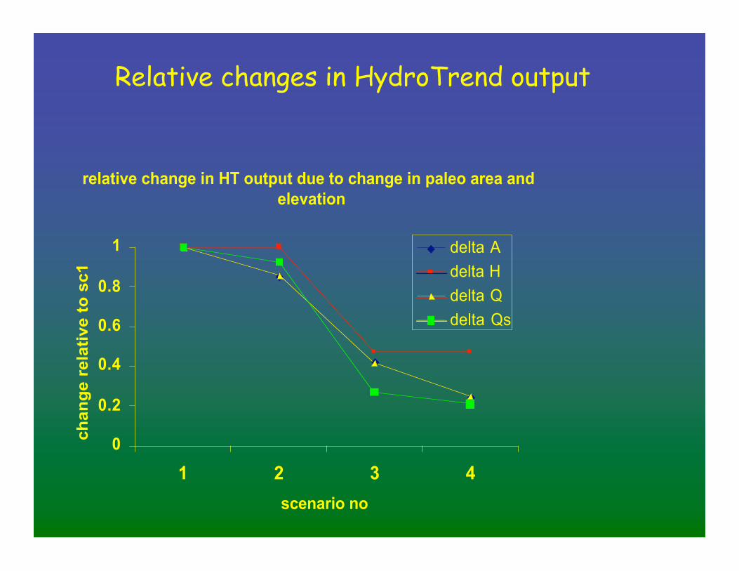
Relative changes in HydroTrend output
relative change in HT output due to change in paleo area and
elevation
0
0.2
0.4
0.6
0.8
1
1 2 3 4
scenario no
ch
an
ge
re
lati
ve
to
sc
1
delta A
delta H
delta Q
delta Qs

SENS 1 SedFlux output - sea floor properties
Sea floor properties differ tremendously between the 2 scenarios,
both in volume and GSD (x)

SedFlux output- GSD(x)
300 year run
- coarsening due to
enlargement of the
estimated drainage basin
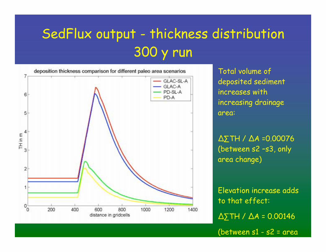
SedFlux output - thickness distribution
300 y runTotal volume of
deposited sediment
increases with
increasing drainage
area:
∆∑TH / ∆A =0.00076
(between s2 –s3, only
area change)
Elevation increase adds
to that effect:
∆∑TH / ∆A = 0.00146
(between s1 - s2 = area

SENS 2; Paleo Temperature and Precipitation:
4 scenarios
Sc1: present-day T minus T-trend of Vostok ice core
Sc2: based on Community Climate Model (CCM1) T and P at the Hudson rivermouth
Sc3: based on Community Climate Model (CCM1)T at the Hudson rivermouth, P in thedrainage basin
Sc4: P based on glaciological modeling (Marshall, 2002)
Concluding ‡ input parameters T and P have huge uncertainty
paleo precipitation 21KBP (CCM data)
0
20
40
60
80
100
120
140
160
180
200
jan feb mar apr may jun jul aug sept okt nov dec
P i
n m
m
Hudson rivermouth
projected Upper Hudson
P based on Glacial model
paleo temperature 21 KBP
-30
-20
-10
0
10
20
30
jan feb mar apr may jun jul aug sept okt nov dec
T i
n g
rd C
Hudson rivermouth
PD-Vostok
PD

Paleo Temperature and Precipitation:
HydroTrend output 300 yr run
Cooling
Effect of lower T (∆T =10 C)
- ∆Q /∆T = 9.6 m3/s / C
- ∆Qs /∆T = 17 kg/s / C
Wettening
Effect of higher P (∆P= 0.5 m)
Higher Q and Qb
∆Q /∆P = 3242 m3/s / m rain
∆Qb /∆P = 65 kg/s / m rain
- No change in Qs

SedFlux output: thickness distribution
- total deposited volume
decreases slightly with T
- total deposited volume
increases with P
- deposited volume is
dominated by P changes as
compared to T changes:
∆TH /∆P = 3777 m / m
∆TH /∆T = -109 m / C
- increase in P mainly
increases floodplain and
bedload sedimentation.

SedFlux output: GSD(t)
change in T estimate (~ 10 C)only results in limited GSD(t) change
change in P estimate (~ 0.5 m)results in more pronounced GSD(t) change

GSD(t)- relative changes
0
0.05
0.1
0.15
0.2
0.25
0.3
0.35
0.4
0.45
0.5
0 5 10 15 20 25 30
distance from rivermouth in km
de
lta
GS
D/d
elt
a P
-0.04
-0.03
-0.02
-0.01
0
0.01
0 5 10 15 20 25 30
distance from river mouth in km
delt
a G
SD
/delt
a T
Precipitation
Temperature
The mean grainsize deposited
over time is more strongly influenced
by changes in P input (~40 %)
than by changes in T input (~ 3%)

SENS 3: Storm experiments
New Jersey Shelf at present-day heavily influenced by storm ‡quantify what variability this introduces
Experiments:
Storm 0 = no storms
Storm 1 = Kdiff 0.75, Storm Mag 4
Storm 2 = Kdiff 1.5, Storm Mag 8
Storm 3 = Kdiff 3, Storm Mag 8
Storm 4 = Kdiff 10, Storm Mag 8
Storm 5 = Kdiff 20, Storm Mag 8
Storm 6 = Kdiff 50, Storm Mag 8
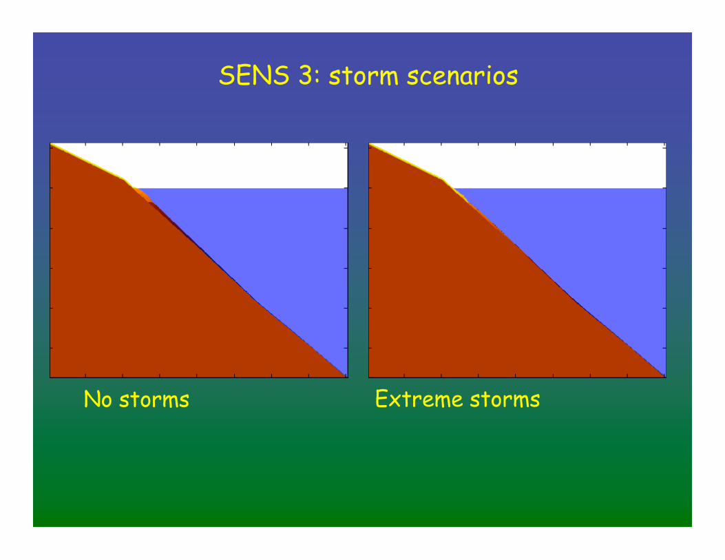
SENS 3: storm scenarios
No storms Extreme storms

SedFlux output: X-section bulk density

SedFlux output; geometric attribute
Thickness distribution
Extreme storms
No storms
∆Th prediction

++++180-460%10% -----------0-1200Ocean storms
+22%26%
Q = 210%
Qs = -15%0.5 mPrecipitation
+/--15% - 22%21%
Q = 8%
Qs = 45%10 CTemperature
+/ -
++
< 5%
10-20%
16%
36%
14%
18%
35k +/- 5k
140k +/- 50k
Area
due LIS/SL
influence
SEDFLUX
Pseudowells
SEDFLUX
Variability
_ GSD(t)
SEDFLUX
Geometry
mean TH
HydroTrend
(Qs)
Input -
Range
CLIMATIC
BOUNDARY
CONDITION
SUMMARIZING TABLE

SedFlux output; volume attribute GSD(x)
5cm-bins


dep
thd
ep
th
var GSD in phi var GSD in phi

50 cm
Entire sediment column
(5m)
10 cm

GSD-variance along the longitudinal
profile for different depth-zones

Thick storm beds
resolved
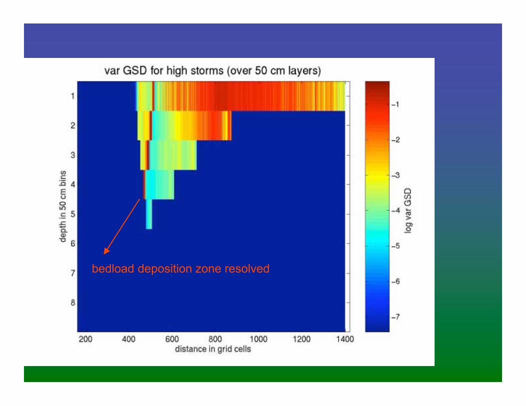
bedload deposition zone resolved
Conclusions
• SedFlux is able to predict long-term stratigraphic patterns
(geometry and thickness at 100m longitudinal resolution and physicalproperties at 10 cm depth resolution).
• To make relevant predictions for acoustic properties HydroTrend andSedFlux need to be integrated and used at daily time-step to capturepeak-flows and storms.
• High-resolution input data are increasingly online available on globalscale (e.g. present-day climate, paleo from CCM) but the associateduncertainties can be significant. This does not necessarily propagateinto the sea floor properties prediction.
• SedFlux provides a method to quantify variability due to uncertaintiesin the boundary conditions by running different input scenarios.
A high-resolution output matrix can be associated with differentresolution layer models of variance in data (e.g. variance of GSD in
50 l )