selecting public goods institutions: who likes to punish
TRANSCRIPT
No. 12-5
Selecting Public Goods Institutions: Who Likes to Punish and Reward?
Michalis Drouvelis and Julian C. Jamison
Abstract: The authors extend the standard public goods game in a variety of ways, in particular by allowing for endogenous preference over institutions and by studying the relationship between individual types, their preferences, and later behavior within the various institutional environments. They collect individual data on a variety of demographic factors, in addition to measuring levels of risk aversion and ambiguity aversion (over both gains and losses). The authors then elicit preferences in an incentive-compatible manner over voluntary contribution mechanisms with and without reward and punishment options. Finally, they randomly assign subjects to one of the four institutions and observe repeated play. They find that payoffs are significantly greater when punishment is allowed but that only a small minority of participants prefers such an environment. There is at most a weak link between individual characteristics and elicited preferences over environments. On the other hand, institutional preferences, as well as individual characteristics, are more strongly predictive of behavior in the public goods game. For instance, loss averse individuals preemptively reward more often when that option is available. This result suggests that when studying social interactions, especially if people can choose whether to participate in a sanctions-and-rewards mechanism, it is important to consider individual attitudes toward risk and uncertainty. Keywords: public goods; voluntary contribution; risk, loss, and ambiguity aversion; preference elicitation; reward and punishment JEL Classifications: C92; H41; D81 Michalis Drouvelis is a lecturer in the department of economics at the University of Birmingham. His e-mail address is [email protected]. Julian C. Jamison is a senior economist at the Federal Reserve Bank of Boston. His e-mail address is [email protected]. The authors thank Jeff Butler, Antonio Cabrales, Urs Fischbacher, Simon Gächter, Brit Grosskopf, Zack Grossman, John Hey, and participants at the Southern Economic Association meetings and the 2012 IMEBE conference for helpful comments; Lynn Conell-Price for research assistance; Walter Yuan for programming assistance; and the University of York for financial assistance. Remaining errors are due solely to the authors. This paper, which may be revised, is available on the web site of the Federal Reserve Bank of Boston at http://www.bostonfed.org /economic/wp/index.htm. This paper presents preliminary analysis and results intended to stimulate discussion and critical comment. The views expressed herein are those of the authors and do not indicate concurrence by the Federal Reserve Bank of Boston, or by the principals of the Board of Governors, or the Federal Reserve System. This version: June 5, 2012
1
I. Introduction Institutions are an integral part of our social life and organize important aspects of
economic activity. It is well-established that different institutions lead to different economic
outcomes (North 1990). How institutions are shaped also has serious implications for the
evolution of human culture and societies (Tabellini, 2008). Due to economic, political, social,
and geographical reasons, different societies select different rules to govern their institutions and
the development of institutional rules over time impacts a nation’s economic performance and
prosperity. For example, Acemoglu, Johnson, and Robinson (2001, 2002) show that the adoption
of different colonization strategies and policies have led to differences in the institutions
implemented in the respective colonized countries, which consequently have affected their long-
run economic welfare. In related work, by using a large sample of countries Easterly and Levine
(2003) and La Porta et al. (1998) demonstrate that institutions can explain differences in the
levels of a country’s economic development and financial performance, respectively. Thus, our
understanding of how institutional structures are selected and established, as well as what factors
are predictive of this process, are of great interest for economists and social scientists.
In this paper, we use experimental methods to shed more light on these questions and to
gain a better understanding of how the underlying institutions enforce a society’s norms. We
focus on institutions that are concerned with providing public goods in settings where free-riding
incentives are present. The general motivation for studying these institutions stems from the fact
that a number of real-life situations (for example, tax compliance, donations to charities, tipping
in restaurants, and participation in collective actions) are characterized by an incentive structure
where people’s individual and collective goals are at odds. This tension is starkly isolated in the
public good environments we examine. In addition, experimental behavior in these institutions
has inspired the recent development of novel theoretical models of social preferences (see
Camerer 2003) which account for a number of the observed anomalies. Therefore, identifying
which forces determine the content of acceptable standards of behavior captured by these
institutions will shed further light on the proximate sources of human cooperation. It will also
improve our inadequate understanding of how social norms are formed and enforced, insofar as
those norms arise from self-selection into groups that prefer certain modes and rules of
interaction. Our aim is to design an experiment which will provide a complete analysis of the

2
processes underlying the way that people make decisions in public good institutions by
separating the conflict between personal and collective gains.
A more specific motivation for our study comes from a burgeoning experimental
literature that investigates individuals’ voting preferences over public good institutions and over
the specific rules that govern these institutions. A main message from these studies (see the
related literature section for a more extensive review) suggests mixed evidence on which
institutions people favor, but in general it is observed that democratically selected institutions (by
using a certain voting rule) perform better than institutions that have been exogenously imposed,
both in terms of average contribution levels and efficiencies measured by net earnings. Yet the
existing literature does not address two important issues in settings involving public goods. First,
which institutions do individuals actually prefer? Second, which individual characteristics have
predictive power over their preferred institutional choice and of behaviors in the relevant
institutions?
Recent experimental studies typically implement a voting mechanism in order for
individuals to express their institutional preferences. However, at least two difficulties arise
when individuals cast their votes. First, voting may not necessarily provide an accurate measure
of which institutions individuals actually prefer. When individuals vote for a certain institution,
subsequent strategic considerations among individuals are likely to be taken into account, which
in turn may confound voting behavior. For example, subjects may consider the behavior of other
voters and vote strategically, a result that may lead to behavior that contradicts their authentic
preferences over a given institution. Second, voting has the drawback of not allowing individuals
to express the intensity of their preferences, making it impossible to draw conclusions about the
strength of their approval or disapproval.
Our paper presents a novel experiment which introduces an incentive-compatible
mechanism to elicit preferences over a menu of four institutions, each with different enforcement
mechanisms to punish and/or reward behavior that does not comply with a certain norm: a
standard voluntary contributions mechanism (VCM), a VCM with opportunities to sanction, a
VCM with opportunities to reward, and a VCM with opportunities to sanction and reward. To
elicit individual preferences, we ask subjects to indicate which institution they prefer by
indicating how much each institution is worth to them. The stated monetary amount is subtracted

3
from their total earnings if they are assigned to an institution they prefer, and it is added to their
total earnings if they are assigned to an institution they do not prefer. By observing how
individuals select institutions from the available set of options, we are able to draw conclusions
about which enforcement mechanism is actually preferred. By observing how much individuals
are prepared to pay or how much they would need to be paid to participate in a given institution,
we elicit the intensity of their preferences.
To the best of our knowledge, our paper is the first experimental study which elicits
preferences regarding public good institutions and the intensity of these preferences in an
incentive-compatible manner.1 Our study also contributes to the understanding of social norms
by simultaneously analyzing the three enforcement mechanisms that have played a central role in
the social preferences literature. As a control case, we include an institution where neither
sanctions nor rewards are present. The comparison of behavior among the three institutions using
different enforcement mechanisms enables us to disentangle which particular institutional aspect
(sanctions and/or rewards) of an institution, if any, is important for sustaining norms of high
cooperation and maximizing individuals’ overall welfare. We believe that the use of laboratory
experiments is ideal for addressing these questions, as collecting data on our variables of interest
is often infeasible in naturally occurring environments. Additionally, incentivizing preferences
and assessing efficiency issues is typically difficult in the field due to a number of factors that
operate simultaneously, confounding the analysis of causal relationships.
Furthermore, the level of tight control provided by experimental methods allows us to
elicit a number of variables that we hypothesize may influence subjects’ choice of institutions
and subsequent play. Our central focus is on preference measures, such as risk, loss, and
ambiguity aversion, an interest that stems from the fact that a high degree of uncertainty and
ambiguity about the effect of a rule change might lead to a change in an individual’s earnings.
For example, institutions with punishment options have the potential to be detrimental (or at least
add variability) to subjects’ welfare and thus may be preferred by risk-seeking subjects. In
1 Technically we need to be a bit careful about the exact usage of incentive-compatibility in this paper. The ordinal rankings are clearly incentive-compatible, and the cardinal rankings (intensities) have the right relative ratios within an individual, but may be compressed in absolute levels due to risk aversion. Cardinal preferences are always hard to compare across individuals, and that is even more true here due to potential differences in risk attitudes. In practice, as reported below, we do not see any empirical relationship between risk aversion and the absolute value of expressed intensities (not surprisingly given the stakes), so this absence is unlikely to cause any issues when interpreting the results.

4
contrast, institutions with reward mechanisms may be preferred by individuals who are averse to
ambiguity. Also, loss averse and risk averse individuals may be attracted to institutions where
sanctions and rewards are not available.
Our decision to focus on attitudes toward uncertainty is driven not just by the conceptual
arguments above, but also by previous studies that found such a link in other institutional
settings. Laboratory studies such as Bartling et al. (2009) and Dohmen and Falk (2011) have
found that subjects who are less risk-averse are more likely to sort into competitive environments
or variable-pay schemes. Similarly, Weinhold and Zak (2005) find that risk attitudes are central
to wage-related occupational choice in China. Cramer et al. (2002) exhibit a negative
relationship between risk-aversion and entrepreneurship and argue for causality, which is never
absolutely clear but certainly follows if risk attitudes are stable, as in standard theory. Finally and
perhaps most relevantly, there is a relatively long history in the contract theory literature
studying the link between risk tolerance and contract choice, going back at least to Cheung
(1969). A striking recent example is Ackerberg and Botticini (2002), who examine agricultural
institutions in Renaissance Italy and show that risk-sharing is a major determinant of contract
choice.
Although the papers described above are suggestive, the relationship between risk
tolerance and social preferences, including voluntary contributions, has received relatively scant
direct attention. There have been a few experimental studies (for example, Eckel and Wilson
2004; Humphrey and Renner 2011; Kocher et al. 2011), that have yielded equivocal evidence.
Importantly, all these studies overlook the possibility that preferences other than standard risk
preferences, such as loss and ambiguity aversion, may predict social preferences. These studies
also do not credibly elicit preferences over specific social mechanisms for procuring public
goods. In our paper, we elicit choices in order to construct four preference measures (risk
aversion, loss aversion, ambiguity aversion, and ambiguity aversion over losses) in an incentive-
compatible manner, and we provide the first comprehensive analysis of how these preference
measures can predict subjects’ reciprocal behavior in the form of punishing or rewarding their
peers.
Our main findings can be summarized as follows. First, our four preference measures are
significantly correlated with each other. Second, subjects’ individual characteristics help explain

5
their preferences over risk, loss, and ambiguity. Third, which institutions individuals prefer are,
surprisingly, not influenced by preference measures, although other individual traits do have
some explanatory power. Fourth, institutions with punishment options are best able to maintain
cooperative norms. Fifth, relative to institutions without sanctioning mechanisms, institutions
that permit sanctions incur enforcement costs that lower overall welfare in the short run but
increase overall efficiency in the long run. Sixth, positive and negative reciprocity are
significantly correlated with our preference measures. Seventh, subjects’ individual
characteristics account for the way sanctions and rewards are used.
The remainder of the paper is structured as follows. Section 2 reviews the related
literature. Section 3 outlines our experimental design and section 4 presents the results from our
data analysis. Section 5 concludes by discussing the implications of our results and how these
might be extended by further work.
II. Related Literature
Our paper contributes to three different strands of literature: a) classical public goods
experiments; b) endogenous selection of environments; and c) the interaction of preference
measures and social preferences. We discuss the related literature for each of these three lines of
research in turn. Readers familiar with the extensive literature on public goods games can skim
most of this section, but we hope that it will provide a useful survey for others, in addition to
placing our contribution in context with the existing literature.
1. Classical public goods games: Over the last 40 years of experimental economic research, there
has been extensive exploration of how people behave in decision situations where a tension
exists between personal and collective gains. By now it is well-understood that actual behavior
does not conform to standard economic theory’s sharp prediction that people will free ride. The
stylized facts emerging from these experiments suggest that, on average, individuals initially
contribute between 40 percent and 60 percent of their endowment, but contributions gradually
decline as the game progresses. The erosion of cooperation with repeated interactions is robust to
variations in experimental design—for instance, whether group composition is constant or
randomly changes over time (see, for example, Keser and van Winden 2000; Andreoni and
Croson 1998), or whether the group size changes (see for example, Isaac and Walker 1998a).

6
These findings have been widely documented in numerous experiments, which are
comprehensively surveyed by Ledyard (1995) and Gächter and Herrmann (2005). Intrigued by
the fragility of cooperation, many economists have sought to identify mechanisms in order to
remedy the free-rider problem. Thus far, a number of different processes that are able to sustain
the norm of high contributions have been proposed. Principally, these include the introduction of
sanction and reward possibilities (for example, Fehr and Gächter 2000, 2002; Noussair and
Tucker 2005; Sefton, Shupp, and Walker 2007; Sutter, Haigner, and Kocher 2010); third-party
punishment (for example, Fehr and Fischbacher 2004; Carpenter and Matthews 2012);
expressions of disapproval (for example, Gächter and Fehr 1999; Masclet et al. 2003; Rege and
Telle 2004); the threat of expelling group members (for example, Cinyabuguma, Page, and
Putterman 2005); the establishment of leaders (for example, Güth et al. 2007; Levati, Sutter, and
van der Heijden 2007); assortative matching (for example, Gächter and Thöni 2005); and
communication among players (for example, Isaac and Walker 1988b; Bochet, Page, and
Putterman 2006).
In our paper, we focus on public good environments where individuals have the opportunity
to punish and/or reward their peer group members. Since Fehr and Gächter’s seminal 2000 paper
introduced the punishment mechanism, a growing literature has been generated to examine the
effect that punishment has on cooperation (see Chaudhuri 2011 and Gächter and Herrmann 2009
for surveys).2 This work suggests that punishment prevents the decline of contribution levels
observed when sanctioning mechanisms are absent,3 and that punishment promotes efficiency (as
measured by individuals’ net earnings) in the long run but not in the short run (see Gächter,
Renner, and Sefton 2008). Another important finding of this literature is that individuals are
willing to spend their own resources in order to lower the income of those peer group members
who violate reciprocity norms. As a natural extension of findings on negative reciprocity,
economists have also explored the effect of a reward mechanism in promoting cooperative
behavior. Recent laboratory studies have shown that when the cost-to-impact ratio of rewards is
2 In disciplines other than economics, the implications of punishment have also received considerable attention (see, e.g., Yamagishi 1986; Ostrom, Walker, and Gardner 1992; de Quervain et al. 2004). 3 It is also worth mentioning that punishment’s cooperation-enhancing effect can be eradicated in the presence of antisocial punishment (see Herrmann, Thöni, and Gächter 2008; Gächter and Herrmann 2009, 2011); second-round punishment opportunities (see Cinyabuguma, Page, and Putterman 2006; Denant-Boemont, Masclet, and Noussair 2007; Nikiforakis, 2008); and its cost and effectiveness (see Anderson and Putterman 2006; Carpenter 2007, Egas and Riedl 2008; Nikiforakis and Normann 2008).

7
1:1, the reward mechanism is unable to sustain cooperation either in repeated interactions
(Sefton, Shupp, and Walker 2007) or in a one-shot environment (Walker and Halloran 2004).
However, when the benefit of receiving a reward exceeds the cost of assigning it, there is
evidence that rewards can also be effective in sustaining cooperation (e.g., Vyrastekova and van
Soest 2008; Drouvelis 2010).
A common feature of the studies cited above is that the public good environments have been
determined exogenously. In other words, the experimenter randomly assigns the participants to
one institutional environment, so subjects do not select the environment they prefer to play in. A
recent line of research has departed from this standard design to examine subjects’ behavior
when they are allowed to choose the environment in which they would like to interact. Our
experiment contributes to this recent research, and we discuss the relevant literature in the next
subsection.
2. Endogenous selection of environments. While our discussion will center on the literature
addressing endogenous selection of public good structures, it is worth mentioning that
endogenous selections of environments have been experimentally explored in other contexts.
These include prisoner’s dilemma games (Bohnet and Kübler 2005), dictator games (Lazear,
Malmendier, and Weber 2012), auctions (Palfrey and Pevnitskaya 2008; Jamison and Karlan
2009), incentive pay schemes (Eriksson and Villeval 2008; Dohmen and Falk 2011), and
competitive environments (Niederle and Vesterlund 2007; Bartling et al. 2009). With respect to
public good environments, the experimental literature has focused on the selection of
environments that offer rewards and punishments.4 For example, in a study by Botelho et al.
(2005) subjects were asked to vote for their preferred environment after they acquired experience
by playing for 10 periods in each of the available environments (a standard public good game
and a public good game with sanctioning opportunities). After the voting took place, the majority
of votes determined which environment all subjects played in for a final period.5 This study
found that subjects did not favor the sanctioning environment and also found that sanctions did
not have a sustained positive effect on contributions and profits.
4 A notable exception is Potters, Sefton, and Vesterlund (2005) who conducted an experiment in which subjects voted on whether they preferred a simultaneous versus a sequential public good game with imperfect information. Their subjects preferred the sequential ordering to the simultaneous one. 5 To make the voting decision salient, subjects’ earnings in the final period were 10 times more those of each of the first 20 periods.

8
Another experiment by Gürerk, Irlenbusch, and Rockenbach (2006) had subjects vote at the
beginning of every period whether they would like to play in an environment without or with
sanctions (both positive and negative). In each period, a participant then interacted with all the
other participants who had chosen the same institution. Their results provide evidence that given
a “voting-with-one’s-feet” approach the sanctioning environment becomes the predominant
choice over time. In a later paper, Gürerk, Irlenbusch, and Rockenbach (2009) provide further
evidence that when subjects are confronted with a choice between an environment with or
without punishment, the environment with punishment gradually becomes the dominant choice.
In both of their studies, the environment where sanctioning opportunities were available led to
higher contribution and efficiency levels.
Sutter, Haigner, and Kocher (2010) examined how endogenous selection affected three
public goods environments (a standard public good game, a public good game with punishment,
and a public good game with rewards) by letting subjects vote whether or not to accept each of
the available environments. Voting was optional and costly to those who decided to participate.
If one environment received unanimous support, it was played by all subjects in all periods; if
multiple institutions were unanimously supported the tie was randomly broken. If unanimity was
not achieved on the first vote, subjects continued voting until one environment was unanimously
chosen. Their findings suggest that institutional preferences depend on the cost-to-impact ratio of
the punishment and reward environment. When the ratio was to 1:3, 85 percent of the groups
agreed on the public good game with reward, whereas with a ratio of 1:1, 63 percent agreed on
the standard public good game. In their endogenous treatments, Sutter, Haigner, and Kocher find
that the reward environments (both under a 1:1 and a 1:3 ratio) and the punishment environment
(under a 1:1 ratio) generate higher contribution levels than the standard public good game.6
A number of recent experimental studies have further indicated that democratically selected
institutions have positive effects on behavior. Ertan, Page, and Putterman (2009) find that
institutional environments where subjects vote on whom they are allowed to punish (meaning,
below-average, average, and/or above average contributors) yield higher contributions and
greater efficiencies than institutions in which punishment is unrestricted. In the democratic
institutions, most groups vote to allow punishment of norm violators who undercontribute but do
6 Note that the punishment environment with a ratio of 1:3 was never agreed to be played.

9
not sanction high contributors (those whose contribution exceeds the norm). In another study,
Putterman, Tyran, and Kamei (2010) provide evidence that giving subjects the opportunity to
vote on the penalty structure (meaning, whom to penalize and the strength of sanctions) in an
environment that allows punishment will lead to efficiency-enhancing outcomes relative to an
environment where subjects are not given this opportunity. Kamei (2011) also finds that when a
sanctioning policy is implemented democratically, subjects who favor the policy contribute more
to their group than subjects who favor the policy contribute when the policy is implemented
exogenously. In another series of experiments, Dal Bó, Foster, and Putterman (2010) also show
that letting subjects democratically choose which policy they prefer positively affects
cooperative behavior.
A clear message from this literature is that voting is the prevalent procedure used to
implement individuals’ preferences over environments. Although voting is a valid method for
endogenously assigning individuals to specific environments, its disadvantage is that voting is
not necessarily an incentive-compatible process. Our experimental investigation contributes to
the “endogenous selection” literature in at least two respects. First, as described briefly in the
introduction and in detail below, we introduce a fully incentive-compatible mechanism to elicit
preferences over different public good environments. Second, our design consists of all four
possible environments (a standard public good game, a public good game with punishment, a
public good game with rewards, and a public good game with punishment and rewards), thus
allowing us to compare their relative appeal as well as to disentangle the different individual and
collective incentives that might be at work in these environments. Further, since we randomize
assignments, we can separate the effect of selection from the effect of the institutional rules per
se.
3. The interaction of preference measures and social preferences. This topic has received little
attention in the literature. A few experimental studies have recently addressed how preference
measures interact with social preferences, but evidence from the available studies is mixed and
focuses mainly on trust games. In a trust game in rural Paraguay, Schechter (2007) shows that
risk aversion plays an important role in determining behavior, whereas Eckel and Wilson (2004)
find no significant relationship between risk measures and the decision to trust. In another
experiment, Kocher et al. (2011) provide evidence that there is no correlation between risk
preferences and behavior in a public good game and in a trust game.

10
These experiments mainly address the issue of whether and how behavior in games
measuring social preferences is affected by preference measures. While this is a relevant research
question to identify the factors influencing prosocial behavior, another important question largely
ignored in this literature is what motivates the demand for different public good environments.
This is a significant omission, as better understanding the self-selection process can help us
improve the design of public institutions that promote social welfare and cooperation. By
designing a novel experiment which elicits preferences over a menu of public good institutions in
an incentive-compatible manner, our paper systematically investigates whether and how
individual preferences affect the choice of institutions and subsequent behavior.
III. Experimental Design
Our experiment was conducted in two parts. In the first part we elicited subjects’ levels of
risk and ambiguity aversion (over both gains and losses). In the second part we elicited
preferences over four public good environments and then randomly assigned subjects to one of
these environments to play a repeated voluntary contribution game. At the beginning of the
experiment, subjects were informed that the experiment would consist of two parts (in order to
reduce the likelihood of incorrect expectations about the nature of the experiment). However,
they were not told what would happen in the second part of the experiment (see Appendix A for
the timeline of tasks that occurred in a session).
In order to elicit their preferences, participants were shown a table with seven rows and asked
to choose between a safe option and a lottery option in each row. The safe option was exactly the
same in each row, but the amount in the lottery option increased from row to row. More
precisely, in the first row subjects could choose to receive £6 with certainty, or they could choose
to play the lottery and have a 50 percent chance of receiving £0 and a 50 percent chance of
receiving £11. Moving down the table, the amount it was possible to win in the lottery increased
to £12, £13, £14, £16, £18, and £20. After a subject had made a decision for each row, it was
randomly determined which row became relevant for payoff. Subjects were informed of their
lottery payment at the end of the experiment. This procedure guaranteed that each decision was
incentive-compatible. The number of times a subject chose the safe option indicates his or her

11
attitudes towards risk; that is, the more times a subject selected the sure payoff of £6, the more
risk averse this subject is.
As our public good environments involve payoffs that are ambiguous and may even involve
losses, we consider it important to elicit individual attitudes towards loss aversion, ambiguity
aversion, and ambiguity aversion with losses.7 To elicit such preferences we implemented a
procedure similar to the last one used to elicit risk preferences. For instance, to elicit individual
attitudes towards losses, we used the exact same table described above but with payoffs shifted
downwards by £3. Thus the lottery payoffs now involved losses, as these consisted of a 50
percent chance of losing £3 and a 50 percent chance of receiving a positive amount. As a
measure of loss aversion, we used the frequency with which a subject chose the safe option. For
the cases of ambiguity aversion with and without losses, we simply replaced the probability of
each outcome, made explicit in the lottery option, with a question mark to indicate that the
probability was unknown. The four tables were shown to subjects in a random order to control
for order effects. In particular, if the risk and loss questions (with 50–50 lotteries) always
preceded the ambiguity questions, we might expect subjects to have a 50–50 prior distribution
over outcomes when considering the ambiguous lotteries. The randomized presentation of these
questions minimized this effect.
After the elicitation of preference measures, subjects received new instructions describing
each public good environment (see Appendix B). In total, we examined four different
environments, each corresponding to a separate treatment, with the individual participants
experiencing only one treatment (a between-subjects design). We refer to our four treatments as:
a) voluntary contributions mechanism (VCM); b) VCM with punishment; c) VCM with reward;
and d) VCM with punishment and reward. In each session, a group of 12 subjects were randomly
assigned across the above treatments to play a 25 period repeated game in groups of four. The
group composition remained the same throughout the session (that is, a partner matching
protocol). Earnings were given in money units for the public good games and we used an
exchange rate of £0.01 per money unit.
7 For control purposes, we wanted to use a symmetric procedure to elicit individuals’ preferences towards risk, loss and ambiguity which prevented us from using an elicitation method similar to that of Holt and Laury (2002).
12
We will begin by describing our baseline treatment, VCM, and comment on the structure of
the remaining treatments in turn.8
a) VCM treatment
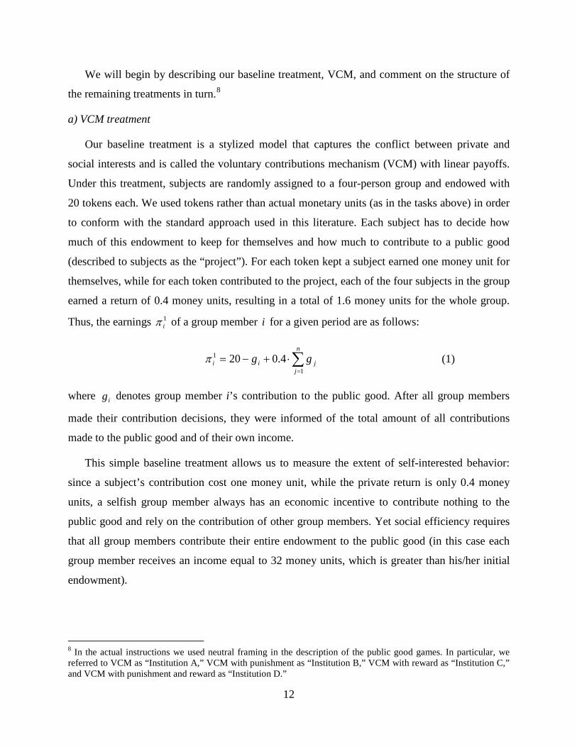
Our baseline treatment is a stylized model that captures the conflict between private and
social interests and is called the voluntary contributions mechanism (VCM) with linear payoffs.
Under this treatment, subjects are randomly assigned to a four-person group and endowed with
20 tokens each. We used tokens rather than actual monetary units (as in the tasks above) in order
to conform with the standard approach used in this literature. Each subject has to decide how
much of this endowment to keep for themselves and how much to contribute to a public good
(described to subjects as the “project”). For each token kept a subject earned one money unit for
themselves, while for each token contributed to the project, each of the four subjects in the group
earned a return of 0.4 money units, resulting in a total of 1.6 money units for the whole group.
Thus, the earnings 1iπ of a group member i for a given period are as follows:
∑=
⋅+−=n
jjii gg
1
1 4.020π (1)
where ig denotes group member i’s contribution to the public good. After all group members
made their contribution decisions, they were informed of the total amount of all contributions
made to the public good and of their own income.
This simple baseline treatment allows us to measure the extent of self-interested behavior:
since a subject’s contribution cost one money unit, while the private return is only 0.4 money
units, a selfish group member always has an economic incentive to contribute nothing to the
public good and rely on the contribution of other group members. Yet social efficiency requires
that all group members contribute their entire endowment to the public good (in this case each
group member receives an income equal to 32 money units, which is greater than his/her initial
endowment).
8 In the actual instructions we used neutral framing in the description of the public good games. In particular, we referred to VCM as “Institution A,” VCM with punishment as “Institution B,” VCM with reward as “Institution C,” and VCM with punishment and reward as “Institution D.”

13
b) VCM with punishment treatment
The VCM with punishment treatment is identical to the VCM treatment except for the
addition of a second stage. After subjects made their contribution decisions during the first stage,
the other three group members’ contribution profiles are revealed at the beginning of the second
stage. No individual subject could identify the particular contribution of any other group
member, since the order of contributions shown in each screenshot randomly changed from
period to period, and therefore, subject-specific reputations could not develop across periods.
Each subject could then assign between zero and five negative points to each of the other group
members. Assigning negative points was costly both to the punisher and the punished group
member, as each negative point costs the punisher one money unit and the punished group
member three money units. Thus, for a group member i for a given period, the total earnings
from both stages, iπ , are as follows:
∑∑≠≠
⋅−−=ij
jiij
ijii pp ,31ππ (2)
where 1iπ denotes the group member i’s payoff from the first stage (as defined in equation 1) and
ijp the number of negative points group member i assigns to group member j.
At the end of the second stage, each subject was informed about the cost incurred for
assigning negative points, the total number of negative points assigned to them, and their
earnings from each period. No information about the number of adjustment points received by
each group member was made available to them, meaning that they did not learn anything about
possible social norms regarding punishment.
c) VCM with reward treatment
The VCM with reward treatment has a similar two-stage structure to the VCM with
punishment treatment. The first stage is identical to the VCM treatment, while in the second
stage, subjects learn the whole vector of individual contributions made in their group during the
first stage. Then each subject is given the opportunity to assign positive points to other group
members—assigning positive points is costly to the donor but beneficial for the recipient. Each
positive point costs the donor one money unit and awards the recipient one money unit. Thus, for
a group member i, the total earnings from both stages, iπ , for a given period are as follows:
14
,11 ∑∑≠≠
⋅+−=ij
jiij
ijii ppππ (3)
where 1iπ denotes the group member i’s payoff from the first stage and ijp the number of
positive points group member i assigns to group member j. The number of positive points that
each group member could assign was between zero and five. As in the previous treatments,
subjects received information about their own rewards and earnings but group information was
not provided.
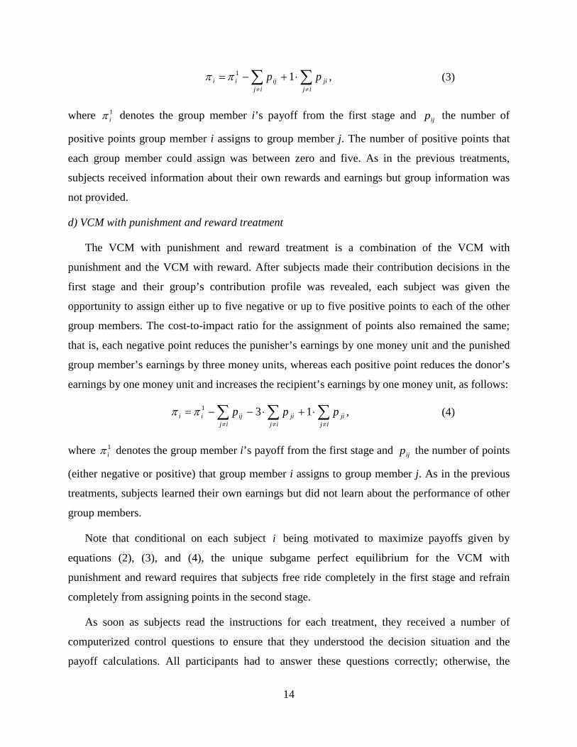
d) VCM with punishment and reward treatment
The VCM with punishment and reward treatment is a combination of the VCM with
punishment and the VCM with reward. After subjects made their contribution decisions in the
first stage and their group’s contribution profile was revealed, each subject was given the
opportunity to assign either up to five negative or up to five positive points to each of the other
group members. The cost-to-impact ratio for the assignment of points also remained the same;
that is, each negative point reduces the punisher’s earnings by one money unit and the punished
group member’s earnings by three money units, whereas each positive point reduces the donor’s
earnings by one money unit and increases the recipient’s earnings by one money unit, as follows:
,131 ∑∑∑≠≠≠
⋅+⋅−−=ij
jiij
jiij
ijii pppππ (4)
where 1iπ denotes the group member i’s payoff from the first stage and ijp the number of points
(either negative or positive) that group member i assigns to group member j. As in the previous
treatments, subjects learned their own earnings but did not learn about the performance of other
group members.
Note that conditional on each subject i being motivated to maximize payoffs given by
equations (2), (3), and (4), the unique subgame perfect equilibrium for the VCM with
punishment and reward requires that subjects free ride completely in the first stage and refrain
completely from assigning points in the second stage.
As soon as subjects read the instructions for each treatment, they received a number of
computerized control questions to ensure that they understood the decision situation and the
payoff calculations. All participants had to answer these questions correctly; otherwise, the

15
experiment would not proceed. Next, subjects were asked to indicate on a percentage scale how
much they expected to earn relative to the maximum potential earnings, considering only
earnings from the 25 rounds of the public good game (see figure C.1 in Appendix C for a
screenshot of this step). We are interested in this assessment as a means to find out whether—
and if so how— overconfidence affects the selection into public good games. Subjects received a
bonus based on the accuracy of their estimation. In particular, if their estimation was within 10
percentage points in either direction of their actual earnings (calculated as a percentage of the
maximum earnings), they received £1; if their estimation was within 15 percentage points in
either direction of their actual earnings, they received £0.50, and if their estimation was within
25 percentage points in either direction, they received £0.20. Subjects were informed about their
true rank in the distribution at the very end of the experiment.
After the subjects answered the overconfidence question, their institutional preferences were
elicited. During this phase, the subjects were asked to indicate in which public good institution
they preferred to participate by quantifying how much each institution was worth to them (in
pounds and pence). The incentive system was as follows: subjects were asked to indicate a
monetary amount for their preferred institution. They were told that if they were assigned to one
of the institutions that they indicated they were willing to pay for, then the monetary amount they
indicated would be subtracted from their final payment. If they were assigned to an institution for
which they had indicated that they would need to be paid to participate in, then the monetary
amount they stated would be added to their final payment. Note that the maximum amount they
could state was any number (with two decimals places) from –£5 to £5 (inclusive) and that the
sum of all four amounts was required to sum to 0. To control for order effects, each institution
appeared onscreen in a random order across participants. Figure C.2 in Appendix C provides a
screenshot of the interface we used for eliciting subjects’ preferences for each institution.
Our incentive mechanism allowed subjects to truthfully express the ordinal ranking of their
preferred institution as well as the strength of their preference (by stating a pound value for the
amount that their preferred structure was worth to them). As long as subjects have diminishing
marginal utility for money (that is, they would prefer to be given money in a low-income state of
the world even if an equivalent [probability-weighted] amount were taken away in a high-income
state), this mechanism induces them to state that they prefer exactly those environments in which
they expect to earn more. On a related note, this elicitation procedure does add additional ex ante

16
uncertainty to their payoffs, so one might worry that the magnitude of the expressed preferences
was a function both of actual underlying intensity and of risk aversion. However, when we
regressed the average absolute value of the expressed preferences against the normalized risk,
loss, and ambiguity attitudes, we found no relationship—suggesting that this was not a concern
in practice.
After subjects entered their relative preferences, they were informed which of the four
environments they had been assigned to and then played the game for 25 rounds. In order to
collect the same amount of independent observations for each treatment, subjects were randomly
allocated to one of the four treatments before the experiment began. After the 25 rounds of play
concluded, subjects were informed of their payoff from the lottery task, the overconfidence
question (along with their actual rank in the distribution), and their earnings from the public good
game. At this point we also collected data on the subjects’ demographic characteristics (such as
gender, age, nationality, marital status, father’s education, political and religious affiliations) and
on a self-control task that is correlated with cognitive outcomes (see Frederick 2005).
Procedures
We conducted sixteen sessions, four sessions for each of the four treatments. A total of 192
subjects participated in the experiment and in each of the four treatments there were 48 subjects.
All the subjects were recruited at the University of York, using the ORSEE software (Greiner
2004). The vast majority of participants were undergraduate students from various academic
fields. The experiment was conducted in the Centre for Experimental Economics (EXEC) lab
and all treatments were computerized and programmed with the Multistage software from
Caltech. The instructions for the elicitation of risk preferences and the description of the public
good environments are provided in Appendix B. Some of the instructions were presented on the
computer screen. At the end of a session, subjects were paid in private according to their total
earnings from all relevant tasks. Average earnings per treatment were as follows: £13.54 for the
VCM, £13.80 for the VCM with punishment, £14.19 for the VCM with reward, and £14.62 for
the VCM with punishment and reward (at the time of the experiment £1 was equivalent to
$1.61). Sessions lasted, on average, 70 minutes, with no session taking more than 90 minutes.

17
IV. Results
In the following three subsections, we present the main results from our experiment. In the first
subsection, we examine the responses that indicated the subjects’ individual attitudes towards
risk, loss, and ambiguity and how these preferences are interrelated and related to the subjects’
personal characteristics and demographics. In the second subsection, we investigate how
preference measures affect the subjects’ choice of institutions. In the last subsection, we focus on
behavior in the public good games, both in contribution levels and in the assignment of points for
punishment and rewards.
1. Preference measures, cognitive reflection test (CRT) questions, and demographics
In the first part of our experiment, we elicited subjects’ risk, loss, and ambiguity
preferences. Recall that for a given preference measure, subjects had to make seven separate
choices between a fixed amount safe option and a lottery, in which the payment amount
increased from row to row moving down the table. We use the number of times a subject chose
the safe option as a measure of his/her attitudes corresponding to the specific preference
measure. For example, when eliciting risk preferences, never choosing the risky option indicates
extreme risk aversion, whereas choosing seven risky options indicates extreme risk-seeking
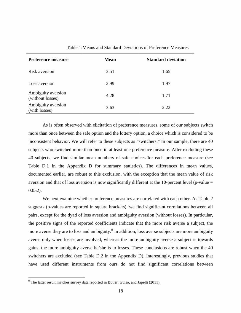
behavior. Table 1 presents summary statistics on how often the subjects chose the sure payoff for
each preference measure. We observe that, on average, our subjects are ambiguity averse both
with respect to both gains and losses. Performing a Wilcoxon matched-pairs signed rank test, we
find that the difference between the mean values of risk aversion and ambiguity (without loss)
aversion is highly statistically significant (p-value = 0.000). This is also the case when we
compare the mean value of loss aversion and that of ambiguity (with losses) aversion (p-value =
0.000). Comparing the mean values of risk aversion and loss aversion, we find significant
differences at the 5-percent level (p-value = 0.038), a result that implies our subjects were more
risk averse than loss averse.
18
Table 1:Means and Standard Deviations of Preference Measures
Preference measure Mean Standard deviation
Risk aversion 3.51 1.65
Loss aversion 2.99 1.97
Ambiguity aversion (without losses) 4.28 1.71
Ambiguity aversion (with losses) 3.63 2.22
As is often observed with elicitation of preference measures, some of our subjects switch
more than once between the safe option and the lottery option, a choice which is considered to be
inconsistent behavior. We will refer to these subjects as “switchers.” In our sample, there are 40
subjects who switched more than once in at least one preference measure. After excluding these
40 subjects, we find similar mean numbers of safe choices for each preference measure (see
Table D.1 in the Appendix D for summary statistics). The differences in mean values,
documented earlier, are robust to this exclusion, with the exception that the mean value of risk
aversion and that of loss aversion is now significantly different at the 10-percent level (p-value =
0.052).
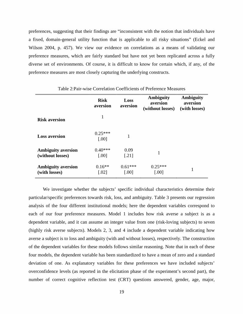
We next examine whether preference measures are correlated with each other. As Table 2
suggests (p-values are reported in square brackets), we find significant correlations between all
pairs, except for the dyad of loss aversion and ambiguity aversion (without losses). In particular,
the positive signs of the reported coefficients indicate that the more risk averse a subject, the
more averse they are to loss and ambiguity.9 In addition, loss averse subjects are more ambiguity
averse only when losses are involved, whereas the more ambiguity averse a subject is towards
gains, the more ambiguity averse he/she is to losses. These conclusions are robust when the 40
switchers are excluded (see Table D.2 in the Appendix D). Interestingly, previous studies that
have used different instruments from ours do not find significant correlations between
9 The latter result matches survey data reported in Butler, Guiso, and Japelli (2011).
19
preferences, suggesting that their findings are “inconsistent with the notion that individuals have
a fixed, domain-general utility function that is applicable to all risky situations” (Eckel and
Wilson 2004, p. 457). We view our evidence on correlations as a means of validating our
preference measures, which are fairly standard but have not yet been replicated across a fully
diverse set of environments. Of course, it is difficult to know for certain which, if any, of the
preference measures are most closely capturing the underlying constructs.
Table 2:Pair-wise Correlation Coefficients of Preference Measures
Risk aversion
Loss aversion
Ambiguity aversion
(without losses)
Ambiguity aversion
(with losses)
Risk aversion 1
Loss aversion 0.25*** [.00] 1
Ambiguity aversion (without losses)
0.40*** [.00]
0.09 [.21] 1
Ambiguity aversion (with losses)
0.16** [.02]
0.61*** [.00]
0.25*** [.00] 1
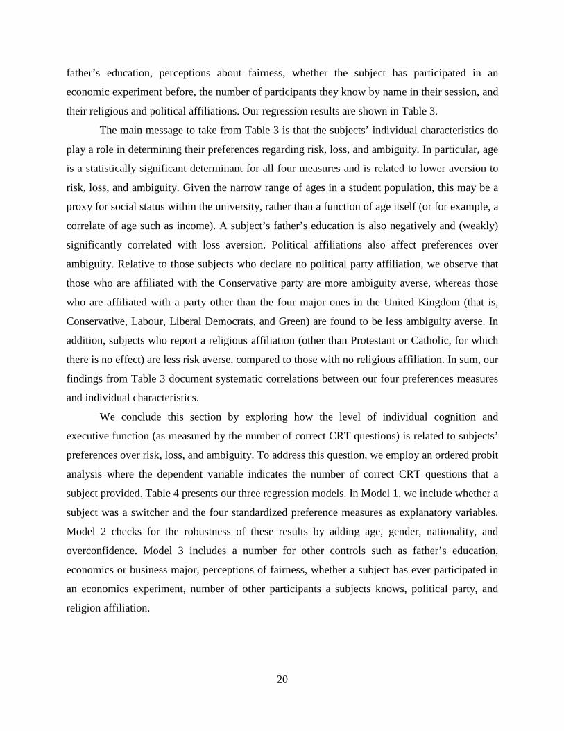
We investigate whether the subjects’ specific individual characteristics determine their
particular/specific preferences towards risk, loss, and ambiguity. Table 3 presents our regression
analysis of the four different institutional models; here the dependent variables correspond to
each of our four preference measures. Model 1 includes how risk averse a subject is as a
dependent variable, and it can assume an integer value from one (risk-loving subjects) to seven
(highly risk averse subjects). Models 2, 3, and 4 include a dependent variable indicating how
averse a subject is to loss and ambiguity (with and without losses), respectively. The construction
of the dependent variables for these models follows similar reasoning. Note that in each of these
four models, the dependent variable has been standardized to have a mean of zero and a standard
deviation of one. As explanatory variables for these preferences we have included subjects’
overconfidence levels (as reported in the elicitation phase of the experiment’s second part), the
number of correct cognitive reflection test (CRT) questions answered, gender, age, major,
20
father’s education, perceptions about fairness, whether the subject has participated in an
economic experiment before, the number of participants they know by name in their session, and
their religious and political affiliations. Our regression results are shown in Table 3.
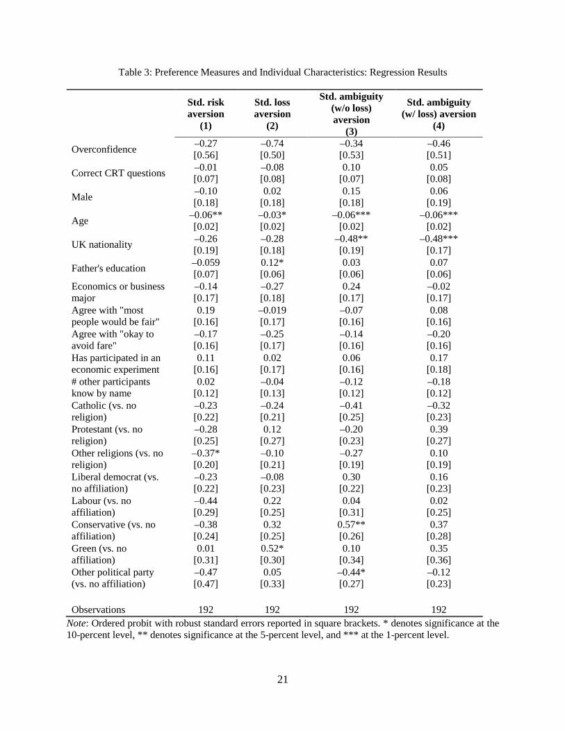
The main message to take from Table 3 is that the subjects’ individual characteristics do
play a role in determining their preferences regarding risk, loss, and ambiguity. In particular, age
is a statistically significant determinant for all four measures and is related to lower aversion to
risk, loss, and ambiguity. Given the narrow range of ages in a student population, this may be a
proxy for social status within the university, rather than a function of age itself (or for example, a
correlate of age such as income). A subject’s father’s education is also negatively and (weakly)
significantly correlated with loss aversion. Political affiliations also affect preferences over
ambiguity. Relative to those subjects who declare no political party affiliation, we observe that
those who are affiliated with the Conservative party are more ambiguity averse, whereas those
who are affiliated with a party other than the four major ones in the United Kingdom (that is,
Conservative, Labour, Liberal Democrats, and Green) are found to be less ambiguity averse. In
addition, subjects who report a religious affiliation (other than Protestant or Catholic, for which
there is no effect) are less risk averse, compared to those with no religious affiliation. In sum, our
findings from Table 3 document systematic correlations between our four preferences measures
and individual characteristics.
We conclude this section by exploring how the level of individual cognition and
executive function (as measured by the number of correct CRT questions) is related to subjects’
preferences over risk, loss, and ambiguity. To address this question, we employ an ordered probit
analysis where the dependent variable indicates the number of correct CRT questions that a
subject provided. Table 4 presents our three regression models. In Model 1, we include whether a
subject was a switcher and the four standardized preference measures as explanatory variables.
Model 2 checks for the robustness of these results by adding age, gender, nationality, and
overconfidence. Model 3 includes a number for other controls such as father’s education,
economics or business major, perceptions of fairness, whether a subject has ever participated in
an economics experiment, number of other participants a subjects knows, political party, and
religion affiliation.
21
Table 3: Preference Measures and Individual Characteristics: Regression Results
Std. risk aversion
(1)
Std. loss aversion
(2)
Std. ambiguity (w/o loss) aversion
(3)
Std. ambiguity (w/ loss) aversion
(4)
Overconfidence –0.27 [0.56]
–0.74 [0.50]
–0.34 [0.53]
–0.46 [0.51]
Correct CRT questions –0.01 [0.07]
–0.08 [0.08]
0.10 [0.07]
0.05 [0.08]
Male –0.10 [0.18]
0.02 [0.18]
0.15 [0.18]
0.06 [0.19]
Age –0.06** [0.02]
–0.03* [0.02]
–0.06*** [0.02]
–0.06*** [0.02]
UK nationality –0.26 [0.19]
–0.28 [0.18]
–0.48** [0.19]
–0.48*** [0.17]
Father's education –0.059 [0.07]
0.12* [0.06]
0.03 [0.06]
0.07 [0.06]
Economics or business major
–0.14 [0.17]
–0.27 [0.18]
0.24 [0.17]
–0.02 [0.17]
Agree with "most people would be fair"
0.19 [0.16]
–0.019 [0.17]
–0.07 [0.16]
0.08 [0.16]
Agree with "okay to avoid fare"
–0.17 [0.16]
–0.25 [0.17]
–0.14 [0.16]
–0.20 [0.16]
Has participated in an economic experiment
0.11 [0.16]
0.02 [0.17]
0.06 [0.16]
0.17 [0.18]
# other participants know by name
0.02 [0.12]
–0.04 [0.13]
–0.12 [0.12]
–0.18 [0.12]
Catholic (vs. no religion)
–0.23 [0.22]
–0.24 [0.21]
–0.41 [0.25]
–0.32 [0.23]
Protestant (vs. no religion)
–0.28 [0.25]
0.12 [0.27]
–0.20 [0.23]
0.39 [0.27]
Other religions (vs. no religion)
–0.37* [0.20]
–0.10 [0.21]
–0.27 [0.19]
0.10 [0.19]
Liberal democrat (vs. no affiliation)
–0.23 [0.22]
–0.08 [0.23]
0.30 [0.22]
0.16 [0.23]
Labour (vs. no affiliation)
–0.44 [0.29]
0.22 [0.25]
0.04 [0.31]
0.02 [0.25]
Conservative (vs. no affiliation)
–0.38 [0.24]
0.32 [0.25]
0.57** [0.26]
0.37 [0.28]
Green (vs. no affiliation)
0.01 [0.31]
0.52* [0.30]
0.10 [0.34]
0.35 [0.36]
Other political party (vs. no affiliation)
–0.47 [0.47]
0.05 [0.33]
–0.44* [0.27]
–0.12 [0.23]
Observations 192 192 192 192
Note: Ordered probit with robust standard errors reported in square brackets. * denotes significance at the 10-percent level, ** denotes significance at the 5-percent level, and *** at the 1-percent level.

22
Table 4: CRT Questions: Regression Results
Dependent variable: # correct CRT
questions 1 2 3
Switcher? –0.56***
[0.21] –0.51** [0.23]
–0.44* [0.24]
Standardized Risk aversion –0.02 [0.09]
0.00 [0.09]
–0.03 [0.10]
Standardized Loss aversion –0.21** [0.11]
–0.16 [0.11]
–0.16 [0.11]
Standardized Ambiguity (w/o loss) aversion
0.10 [0.09]
0.08 [0.09]
0.11 [0.10]
Standardized Ambiguity (w/ loss) aversion
0.14 [0.11]
0.11 [0.10]
0.12 [0.10]
Male 0.31* [0.17]
0.37** [0.18]
Age 0.00
[0.02] 0.00
[0.02]
UK nationality –0.136 [0.17]
–0.07 [0.20]
Overconfidence 1.100** [0.50]
1.09** [0.53]
Controls for other demographics? No No Yes Observations 192 192 192
Note: Ordered probit with robust standard errors reported in square brackets. * denotes significance at the 10-percent level, ** denotes significance at the 5-percent level, and *** at the 1-percent level.

23
Our regression analysis suggests that loss averse subjects appear to correctly answer
fewer CRT questions. However, this effect vanishes when we control for the other demographic
characteristics we collected. Interestingly, these characteristics have a significant impact on our
specific measure of subjects’ cognitive abilities. In particular, we find that males tend to answer
more CRT questions correctly and subjects who report high overconfidence levels also tend to
answer more CRT questions correctly. A noteworthy aspect of our regression results has to do
with the subjects who switched back in at least one of our preference elicitation tasks. In all three
models, it turns out that “switchers” tend to answer fewer CRT questions correctly. The main
findings from this section are summarized in Result 1.
RESULT 1: Preference measures are positively and significantly correlated with each other and
are systematically affected by individual characteristics such as age, nationality, political and
religious affiliations. An individual’s cognitive executive function, as measured by the CRT, are
related to his or her degree of loss aversion, gender, overconfidence, and whether the subject
switched more than once in at least one preference elicitation task.
2. Choice of institutions
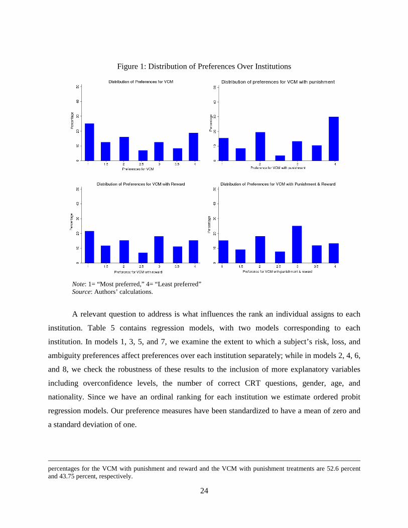
Figure 1 displays the subjects’ distribution of preferences for each of the four institutions.
The horizontal axis in each panel indicates the ranked preference for each institution using a
four-point scale, where “1” denotes a subject’s most favored institution and “4” denotes the least
favored institution. In case of a tie between two or more institutions, we assigned the average
value of the ranked positions that the two institutions occupied. This implies that the sum of the
rankings of each institution for a given subject is always equal to 10.
Most subjects exhibit a preference to participate in institutions which do not include
punishment opportunities. As Figure 1 suggests, the VCM treatment is assigned a ranking of 1,
1.5, or 2 by 53.65 percent of subjects, while the corresponding percentage of subjects who rank
the VCM with reward treatment as 1, 1.5, or 2 is 51.04 percent. On the other hand, the VCM
with punishment and reward, and the VCM with punishment treatments are ranked 1, 1.5, or 2 by
43.75 percent and 40.10 percent of subjects, respectively.10
10 As a complementary measure of preferences, we explored how much each subject was willing to pay/get paid as a percentage of the maximum amount allowed (that is, £5). This analysis conveys a similar message to our earlier discussion. Specifically, 60.42 percent and 53.13 percent of subjects report that they want to pay a non-negative amount to participate in the VCM treatment and the VCM with reward treatment; while the corresponding
24
Figure 1: Distribution of Preferences Over Institutions
Note: 1= “Most preferred,” 4= “Least preferred” Source: Authors’ calculations.
A relevant question to address is what influences the rank an individual assigns to each
institution. Table 5 contains regression models, with two models corresponding to each
institution. In models 1, 3, 5, and 7, we examine the extent to which a subject’s risk, loss, and
ambiguity preferences affect preferences over each institution separately; while in models 2, 4, 6,
and 8, we check the robustness of these results to the inclusion of more explanatory variables
including overconfidence levels, the number of correct CRT questions, gender, age, and
nationality. Since we have an ordinal ranking for each institution we estimate ordered probit
regression models. Our preference measures have been standardized to have a mean of zero and
a standard deviation of one.
percentages for the VCM with punishment and reward and the VCM with punishment treatments are 52.6 percent and 43.75 percent, respectively.

25
Table 5: Preference Measures and Choice of Institutions
Note: OLS regressions with robust standard errors in square brackets. * denotes significance at the 10-percent level, ** denotes significance at the 5-percent level, and *** denotes significance at the 1-percent level.
Dependent variable: ranking of each institution (1, 1.5, ..., 4) VCM rank VCM with punishment rank VCM with rewards rank VCM with punishment &
rewards rank 1 2 3 4 5 6 7 8
Std. Risk Aversion –9.87 (19.05)
–11.88 (19.32)
10.18 (17.69)
10.86 (17.51)
–11.75 (16.51)
–12.97 (16.37)
11.44 (16.41)
13.99 (16.82)
Std. Loss Aversion 5.19 (20.25)
–0.05 (20.56)
13.11 (22.98)
10.71 (23.86)
–9.01 (20.72)
–6.78 (21.07)
–9.30 (19.37)
–3.88 (19.42)
Std. Ambiguity Aversion
18.48 (18.29)
20.04 (19.89)
–9.89 (19.38)
–6.98 (20.58)
–4.81 (19.77)
–5.11 (20.95)
–3.78 (17.44)
–7.94 (18.23)
Std. Ambiguity (with loss) Aversion
–35.31 (22.36)
–30.65 (22.24)
0.293 (22.96)
2.52 (23.63)
8.91 (21.23)
8.24 (21.47)
26.11 (21.93)
19.89 (22.35)
Overconfidence –43.26 (93.90) 67.69
(100.69) 12.85 (93.02) –37.28
(82.33) Correct CRT questions 1.55
(15.27) –32.25** (15.06) 20.11
(13.85) 10.60 (12.90)
Male –35.88 (36.20) 31.92
(40.46) –40.27 (33.59) 44.22
(33.44)
Age –4.26 (4.52) 1.92
(5.09) –0.71 (4.45) 3.05
(4.45)
UK nationality 74.43** (36.96) –10.61
(39.29) 21.13 (36.82) –84.94**
(35.59)
Constant 21.63 (16.10)
118.40 (121.75)
–31.58* (16.29)
–71.88 (131.35)
–8.59 (15.15)
–25.95 (125.60)
18.55 (14.92)
–20.57 (118.16)
Observations 192 192 192 192 192 192 192 192

26
Our regression analysis shows that individual preference measures are not good
predictors of institutional choice, either in terms of magnitude or statistical significance. This
result is robust to several alternate specifications: excluding the 40 subjects who switched
back and forth in at least one preference elicitation task (see Table D.3 in the Appendix);
using the ordinal rather than the cardinal strength of intensity over institutional environments;
and including only one individual preference at a time in the regression (potentially
preferable because of positive correlations between some of those measures). However, the
institutional preference is not simply noise, as can be seen by noting that other individual
variables such as cognitive self-control (as assessed by the CRT task) and UK nationality do
in fact predict it. So although initially we predicted that risk, loss, and ambiguity attitudes
would be important factors at this stage (based in part on previous work as described in the
introduction), we cannot conclude that this is the case.
To further explore this possible relationship, one approach is to look for heterogeneity
within the sample. In particular, note that stating a preference intensity of 500 pence for a
particular institution implies an unrealistically large per-period gain in profits and may be an
indicator that a given subject did not fully understand the situation.11 If we restrict attention
only to those subjects who expressed preference intensities in either direction of 200 pence at
most (there are 135 such subjects from our total of 192), we find instead that being more risk
averse and being more ambiguity averse both significantly predict a preference for the default
VCM institution, meaning the simplest environment with no punishment or reward
mechanisms, as would be expected. This result is robust to the specific cutoffs on intensity
(within a reasonable range), but since this expectation was not our specific hypothesis in
advance we hesitate to give it undue weight. Nevertheless, this result suggests that at least for
some individuals, their attitude toward uncertainty is indeed an important determinant for
their preference towards social structure.
RESULT 2: Overall, preference measures do not seem to matter for institutional choice.
However, further work is warranted to explore the boundaries and extent of this relationship.
11 We thank Urs Fischbacher for suggesting this line of reasoning.

27
3. Behavior in institutions
3.1 Contribution behavior and net earnings
In this subsection, we discuss the results in the first stage of the VCM treatments.
First we present our findings with respect to subjects’ contribution behavior and then we
analyze the efficiency of each of these institutions as measured by the subjects’ average net
earnings.
Figure 2 shows the average contributions made to the public good project across all
25 rounds, smoothed by a five-period moving average. We observe very similar patterns of
average contributions between the standard VCM treatment and the VCM with reward
treatment. In particular, subjects initially contribute approximately 50 percent of their total
endowment, with group allocations declining to roughly 10 percent of the initial endowment
after 25 rounds of play. However, as is apparent in Figure 2, the time trends and average
contributions diverge when we examine the treatments which allow opportunities for
punishment; that is, the VCM with punishment and the VCM with punishment and reward.
Initial average contributions start from approximately the same point relative to the VCM and
the VCM with reward treatments, but as the game progresses the contributions dramatically
increase and move closely together. A visual inspection of Figure 2 suggests pronounced
differences between the punishment and the no-punishment treatments, which are
documented by our statistical analysis reported in Table 6.
Figure 2: Average contributions in each period by treatment
Source: Authors’ calculations.

28
Table 6 presents the p-values of the non-parametric ranksum Wilcoxon test for each
possible comparison between a pair of treatments. In parentheses, we also report the average
contributions for each treatment across all 25 periods. In particular, we observe that the
average contributions are largest in the VCM with punishment and reward treatment (14.73
tokens) and the VCM with punishment (13.74 tokens) and lowest in the VCM (6.25 tokens)
and the VCM with reward treatments (5.86 tokens). Our statistical analysis records
significant differences at the 1 percent level between the treatments with and without
punishment.
Table 6. Average Contributions and p-Values of Pairwise Comparisons
VCM (6.25)
VCM with punishment
(13.74)
VCM with reward (5.86)
VCM with punishment &
reward (14.73)
VCM (6.25) --
VCM with punishment (13.74)
0.00 --
VCM with reward (5.86)
0.66 0.00 --
VCM with punishment & reward (14.73)
0.00 0.73 0.00 --
Notes: Numbers in cells correspond to p-values for each pairwise comparison (using a ranksum Wilcoxon test). Numbers in parentheses correspond to average contributions in each treatment across all 25 periods.
We further examine the efficacy of the treatments with and without punishment by
looking at how average net earnings evolved over time. Figure 3 shows the average profits in
each period in the punishment and the non-punishment treatments, smoothed by a five-period
moving average. Most notably, we see that efficiencies follow a different dynamic across the
treatments. At the beginning of the game the VCMs with punishment yield lower average net
earnings, but as the game progresses the average net earnings increase, resulting in higher
average profits. The opposite pattern is observed in the treatments without punishment. The
net profits are not significantly different between treatments with and without punishment
when we average across all 25 periods (ranksum Wilcoxon test, p-value = 0.503; 24.19
tokens in the punishment treatments and 23.64 tokens in the no-punishment treatments).

29
However, profits are lower (p-value = 0.001) in the first 5 periods of the punishment
treatments (21.93 tokens) as compared to the ones with no punishment (25.45 tokens).
Importantly, this trend is reversed across the final 10 periods, where average net profits are
significantly higher (p-value = 0.016) for the punishment treatments (25.46 tokens) relative to
the treatments with no punishment (22.41 tokens). Our findings provide further support for
previous experimental evidence suggesting that the availability of a punishment mechanism
decreases average net earnings in the short run, but causes an increase in efficiency in the
long run.
Figure 3: Average Earnings in the Treatments with and without Punishment
Source: Authors’ calculations.
To further test that it is the punishment opportunities that cause an increase in the
efficiency of the public good institutions, we also analyze how average net earnings evolved
over time for the treatments with and without reward opportunities. As is apparent in Figure
4, which shows the average profits by period in the reward and the no-reward treatments
(smoothed by a five-period moving average), the average net earnings per subject follow a
similar dynamic across institutional conditions. Averaging across all 25 periods, net profits
are 24.55 tokens in the VCMs with reward opportunities and 23.27 tokens in the VCMs
without reward opportunities. This difference is not statistically significant (ranksum
Wilcoxon test, p-value = 0.452). Nor is any significant difference observed when we look at

30
average net earnings in either the first 5 periods or the last 10 periods. The main findings
from this section are recorded in Result 3.
RESULT 3: The VCM treatments with punishment sustain higher average contribution
levels relative to the no-punishment VCM treatments. The presence of punishment
opportunities causes an increase in efficiency, as measured by average net earnings, in the
long run.
Figure 4: Average Earnings in Treatments with and without Rewards
Source: Authors’ calculations.
3.2 Assigning points for sanctions and rewards
This section analyzes behavior in the second stage of the VCM treatments by
discussing how sanctions and rewards are actually used. Figure 5 depicts how subjects mete
out punishments and rewards based on how much the peer’s contribution deviates from the
punisher’s/donor’s contribution. The vertical axis indicates the average points assigned to a
group member by player i. The horizontal axis indicates the deviation in discrete intervals of
the recipient’s contribution from the contribution of the punisher/donor (player i). For

31
example, a subject in the VCM treatment with punishment assigned, on average, –2.21 points
to those who contributed between 11 and 20 tokens less than him/her.12
Figure 5 provides evidence that in both treatments where punishment opportunities
exist, negative deviations from the punisher are strongly sanctioned. In particular, the greater
the negative deviation is from the punisher’s contribution, the harsher the punishment. Not
surprisingly, in the VCM treatment with reward, we observe that negative deviations are not
rewarded. Positive deviations (using the donor’s contribution as a base) are rewarded, with
the reward being increasing in the size of the deviation. However, for the VCM treatment
with punishment and reward, the average points assigned for positive deviations are half as
much as the average points assigned in the reward only treatment.
Figure 5: Average Points Assigned as a Function of Deviation
from the Sanctioning/Rewarding Player’s Contribution
Source: Authors’ calculations.
To analyze the characteristics of those subjects who assign sanctions and/or rewards,
we employ a multivariate Tobit regression analysis. The dependent variable is the costs an
individual incurs by assigning sanctions and/or rewards in a given period, while the
explanatory variables include the standardized preference measures, the absolute negative
and positive deviations from player i’s contribution (as negative/positive deviations elicit
12 The actual points assigned by the punisher/donor in each deviation interval are shown in Table D.4 in Appendix D.

32
different punishment/reward responses), and other characteristics such as gender, age,
nationality, whether the subject is an economics/business major, overconfidence, and the
number of correct CRT questions. Our regression results are presented in Table 9.
In line with previous results in the literature, we find that absolute negative deviations
are significantly and negatively correlated with the points assigned for punishments and/or
rewards in all three treatments. This result suggests that the more a subject negatively
deviates from the punisher’s/donor’s contribution, the more negative points are assigned to
him/her. In addition, positive deviations are only significantly positively correlated with
points assigned in the VCM treatment with reward, implying that the more a subject
positively deviates from the donor’s contribution the more rewards the donor assigns to
him/her.
Furthermore, we document statistically significant relationships between preference
measures and punishment/reward behavior. Specifically, standardized risk aversion is
positively correlated with the assignment of points in the VCM treatment with punishment,
while loss aversion is significantly and positively correlated with assigned rewards. For the
VCM treatment with punishment and reward, we find that both risk aversion and loss
aversion are significant determinants for assigning points. The more risk averse a subjects is,
the less points he/she assigns; whereas, the more loss averse a subjects is, the more
expenditure he/she makes (by assigning more points).
Finally, our regression results indicate that there is a statistically significant
correlation between UK nationality and point assignment in all three treatments. For the
VCM treatment with reward, we also observe that gender and age are positively and
significantly correlated with assigned rewards, and that those with an economics or business
major reward significantly fewer points than other subjects.
RESULT 4: Preference measures significantly affect the points assigned in all three
treatments. Negative and positive deviations also determine punishment and reward
responses, in the expected direction. Other individual characteristics, such nationality,
gender, age, and economics/business major play a role in how individuals actually use
sanctions and rewards.

33
Table 9: Preference Measures and Assignment of Points: Regression Results
Dependent Variable: Points assigned by player i
VCM with
punishment VCM with reward
VCM with punishment and
reward 1 2 3 4 5 6 Standardized risk aversion 1.15*** 0.85** –0.32 0.02 –0.03 –0.11***
[0.28] [0.34] [0.39] [0.26] [0.05] [0.04] Standardized loss aversion 0.17 –0.20 0.79** 0.29 0.13*** 0.14**
[0.52] [0.42] [0.35] [0.37] [0.04] [0.06] Standardized ambiguity (without loss) aversion
0.05 0.23 0.05 –0.21 0.00 0.05
[0.31] [0.34] [0.29] [0.21] [0.04] [0.04] Standardized ambiguity (with loss) aversion
–0.32 0.15 –0.05 –0.28 –0.02 –0.04
[0.40] [0.50] [0.32] [0.29] [0.03] [0.06] Absolute negative deviation –0.39*** –0.40*** –0.16** –0.19*** –0.13*** –0.14***
[0.07] [0.06] [0.07] [0.06] [0.02] [0.02] Positive deviation –0.06 –0.01 0.22*** 0.22*** –0.01 0.00 [0.04] [0.03] [0.04] [0.03] [0.01] [0.01] Male –0.92 1.16** 0.05 [0.96] [0.52] [0.10] Age –0.07 0.15*** –0.02 [0.06] [0.04] [0.01] UK Nationality 1.40*** –1.24** 0.17** [0.52] [0.54] [0.07] Economics or business major –0.59 –0.90** –0.04
[0.94] [0.44] [0.10] Overconfidence 0.55 –1.29 0.14 [1.45] [1.69] [0.18] Correct CRT Questions –0.04 –0.26 –0.01 [0.29] [0.23] [0.03] Constant 4.05*** 5.78*** –3.42*** –6.36*** 0.01 0.26 [0.76] [2.17] [0.84] [2.00] [0.04] [0.41] Observations 3,600 3,600 3,600 3,600 3,600 3,600 Note: Tobit regressions with standard errors (clustered by matching group) in square brackets. * denotes significance at the 10-percent level, ** denotes significance at the 5-percent level, and *** at the 1-percent level.

34
As a final step, we check to see whether individuals’ underlying preferences over
institutions involving reward or punishment are linked to their ultimate use of reward and/or
punishment. The results of this analysis are reported in Table 10. In addition to the effect of
deviations from one’s own contribution level, as reported above, the most striking finding is
that those subjects who said they preferred a reward environment actually give out
significantly more reward points. Recall that this result is not a selection effect, since
everyone was equally likely to have ended up in the reward setting, and indeed the subjects
are aware that they are matched with people with all different possible preferences.
Nevertheless, these subjects seem to have an underlying belief in the efficacy of rewards to
induce positive behavior (or simply for its own sake). No similar link is found in the case of
punishment.
Table 10: Institutional Preferences and the Assignment of Points for Punishment and Reward
Dependent Variable: Points assigned by player i
VCM with
punishment VCM with reward
VCM with punishment and
reward 1 2 3 4 5 6 Absolute negative deviation –0.40*** –0.15** –0.13*** [0.07] [0.07] [0.02] Positive deviation –0.08 0.22*** –0.01 [0.05] [0.04] [0.01] Ranking of VCM with punishment 0.14 –0.01 [0.29] [0.27] Ranking of VCM with reward –0.41** –0.43** [0.18] [0.19] Ranking of VCM with punishment and reward 0.007 0.01 [0.036] [0.05] Constant 3.16*** 4.08*** –2.36*** –2.46** –0.184* –0.02 [1.19] [1.06] [0.83] [0.97] [0.099] [0.10] Observations 3,600 3,600 3,600 3,600 3,600 3,600
Note: Tobit regressions with standard errors (clustered by independent matching groups) in square brackets. * denotes significance at the 10-percent level, ** denotes significance at the 5-percent level, and *** at the 1-percent level.

35
V. Concluding remarks
This paper provides experimental evidence that a subject’s individual characteristics are
significantly related to his/her economic preferences, which in turn affect behavior in public
goods settings (although surprisingly not the initial institutional preferences). The set of four
institutions we are concerned with in this study are: the standard VCM, the VCM with
punishment, the VCM with reward, and the VCM with punishment and reward. The literature
on public good games suggests the existence of different payoff implications among these
institutions, depending on the rules governing the game. It is therefore a logical inference to
associate preferences over institutions with risk and ambiguity preferences, and to examine
the empirical validity of this relationship. Our novel experimental design also provides us
with a rich dataset which allows us to analyze whether and how preference measures are
correlated with each other, as well as whether these measures gauge the impact of social
preferences such as negative or positive reciprocity. These issues have been relatively less
explored in the literature and our experiment provides a complete set of answers to these
questions in the context of a public good game.
Our paper also demonstrates the significance of individual traits to preference
measures. Although this relationship has recently seen growing interest (see Borghans et al.
2009; Dohmen et al. 2011; Fréchette, Schotter, and Trevino 2011; Butler, Guiso, and Jappelli
2011), these studies limit their attention to particular aspects of individuals’ preferences
(typically risk and ambiguity aversion). We extend this literature by examining four
preference measures: risk aversion, loss aversion, ambiguity aversion, and ambiguity (with
loss) aversion. We show that all four measures are related to a number of individual
characteristics including age, nationality, political and religious affiliations. Interestingly, our
analysis also suggests that our preference measures are strongly correlated with each other,
implying that individuals have a general utility function that is applicable to situations
involving risk and ambiguity. In addition, we find that executive function and cognitive
fluidity, as measured by the number of correct answers to CRT questions, is also associated
with preference measures.
Furthermore, we provide evidence that some individual characteristics are related to
preferences over institutions. The explanation of these preferences is important as they can
have serious implications for a society’s evolution, as well as on its economic performance
and welfare over time. It is therefore important to analyze from an empirical perspective how
institutions are determined. Our findings suggest that most people prefer to participate in
institutions where no sanctioning is present. We also show that the demand for these

36
environments is affected by cognitive sophistication but importantly does not seem to be
affected by attitudes toward risk, loss, or ambiguity.13 Of course, participants had not
experienced any of the environments when making their choices, which was a deliberate
design decision in order to exclude any confounds such as status quo bias, strategic
considerations, or choosing whichever institution happened to have given the highest payoff
based on limited exposure to these environments. A natural avenue for further work is to see
what happens when subjects have amassed some degree of experience with the various
institutional environments. It is also worth pointing out that some previous literature (see
Allen and Lueck 1995 for a review) similarly concludes that there is a weaker relationship
between risk attitudes and contract choice than has been hypothesized by many researchers.
We document significant relationships between reciprocity (whether driven by
strategic concerns or moral disgust) and preference measures. Risk aversion is positively
(negatively) correlated with points assigned in the VCM with punishment (VCM with
punishment and reward), whereas loss aversion is positively related with point assignment in
the VCM with punishment and reward. Our paper confirms and validates previous findings
that although in the short run institutions with sanctions yield lower welfare, in the long run
institutions are more efficient with a punishment mechanism: subjects’ earnings, on average,
are higher relative to the average earnings of those who participate in institutions without
sanctioning options.
Our evidence also suggests some new avenues to enrich the economic theory on
social interactions and the emergence of institutions. For example, recent social preference
models can explain contribution decisions and punishment patterns in public good
environments but lack the ability to incorporate factors such as preference measures and
individual characteristics, which have been shown to have significant predictive behavior.
Our research provides further evidence that risk and social preferences should be
incorporated into economic analysis, as these are related notions that help us further
understand certain aspects of economic behavior. However, additional work remains to be
done in producing a rich body of empirical knowledge in explaining how individual traits
interact with economic preferences.
13 As reported above, we do see some interesting links when the sample is restricted to subjects who are not at the tails of the distribution. Since this was an ex post analysis, we cannot be as statistically confident in it. However, it is reassuringly suggestive for future study.
37
References Acemoglu, Daron, Simon Johnson, and James A. Robinson. 2001. “The Colonial Origins of
Comparative Development: An Empirical Investigation.” American Economic Review
91(5): 1369–1401.
Acemoglu, Daron, Simon Johnson, James A. Robinson. 2002. “Reversal of Fortunes:
Geography and Institutions in the Making of the Modern World Income Distribution.”
Quarterly Journal of Economics 117(4): 1231–1294.
Ackerberg, Daniel A., and Maristella Botticini. 2002. “Endogenous Matching and the
Empirical Determinants of Contract Form.” Journal of Political Economy 110(3):
564–591.
Allen, Douglas W., and Dean Lueck. 1995. “Risk Preferences and the Economics of
Contracts.” American Economic Review, Papers and Proceedings 85(2): 447–451.
Anderson, Christopher M., and Louis Putterman, 2006. “Do Non-Strategic Sanctions Obey
the Law of Demand? The Demand for Punishment in the Voluntary Contribution
Mechanism.” Games and Economic Behavior 54(1) 1–24.
Andreoni, James, and Rachel Croson. 2008. “Partners versus Strangers: Random Rematching
in Public Goods Experiments.” In Handbook of Experimental Economic Results, ed.
By Charles R. Plott and Vernon L. Smith, pp. 776–783. Amsterdam: North-Holland.
Bartling, Björn, Ernst Fehr, Michel André Maréchal, and Daniel Schunk. 2009.
“Egalitarianism and Competitiveness.” American Economic Review, Papers and
Proceedings 99(2): 93–98.
Bochet, Olivier, Talbot Page, and Louis Putterman. 2006. “Communication and Punishment
in Voluntary Contribution Experiments.” Journal of Economic Behavior and
Organization 60(1): 11–26.
Bohnet, Iris, and Dorothea Kübler. 2005. “Compensating the Cooperators: Is Sorting in the
Prisoner’s Dilemma Possible?” Journal of Economic Behavior and Organization
56(1): 61–76.
Borghans, Lex, Bart. H. H. Golsteyn, James J. Heckman, and Huub Meijers. 2009. “Gender
Differences in Risk Aversion and Ambiguity Aversion.” Journal of the European
Economic Association 7( 2–3): 649–658.

38
Botelho, Anabela, Glenn W. Harrison, Lígia M. Costa Pinto, and Elizabet E. Rutström. 2005.
“Social Norms and Social Choice.” Núcleo de Investigação em Microeconomia
Aplicada (NIMA) Working Paper 30. Braga: University of Minho. Available at
http://www3.eeg.uminho.pt/publications/NIMAwp30.pdf.
Butler, Jeffrey V., Luigi Guiso, and Tullio Jappelli. 2011. “The Role of Intuition and
Reasoning in Driving Aversion to Risk and Ambiguity.” CEPR Discussion Paper
8334. London: Centre for Economic Policy Research. Available at
http://www.cepr.org/pubs/new-dps/dplist.asp?dpno=8334.asp.
Camerer, Colin F. 2003. Behavioral Game Theory: Experiments on Strategic Interaction.
Princeton, NJ: Princeton University Press.
Carpenter, Jeffrey P. 2007. “The Demand for Punishment.” Journal of Economic Behavior
and Organization 62(4): 522–542.
Carpenter, Jeffrey. P., and Peter Hans Matthews. 2012. “Norm Enforcement: Anger,
Indignation, or Reciprocity?” Journal of the European Economic Association 10(3):
555–572.
Chaudhuri, Ananish. 2011. “Sustaining Cooperation in Laboratory Public Goods
Experiments: A Selective Survey of the Literature.” Experimental Economics 14(1):
47–83.
Cheung, Steven N.S. 1969. “Transaction Costs, Risk Aversion, and the Choice of Contractual
Arrangements.” Journal of Law and Economics 12(1): 23–42.
Cinyabuguma, Matthias, Talbot Page, and Louis Putterman, 2005. “Cooperation Under the
Threat of Expulsion in a Public Goods Experiment.” Journal of Public Economics
89(8): 1421–1425.
Cinyabuguma, Matthias, Talbot Page, and Louis Putterman. 2006. “Can Second-Order
Punishment Deter Perverse Punishment?” Experimental Economics 9(3): 265–279.
Cramer, J. S., Joop Hartog, Nicole Jonker, and Mirjam Van Praag. 2002. “Low Risk Aversion
Encourages the Choice for Entrepreneurship: An Empirical Test of a Truism.”
Journal of Economic Behavior & Organization 48(1): 29–36.
Dal Bó, Pedro, Andrew Foster, and Louis Putterman. 2010. “Institutions and Behavior:
Experimental Evidence on the Effects of Democracy.” American Economic Review
100(5): 2205–2229.

39
de Quervain, Dominique J.-F., Urs Fischbacher, Valerie Treyer, Melanie Schellhammer,
Ulrich Schnyder, Alfred Buck, and Ernst Fehr. 2004. “The Neural Basis of Altruistic
Punishment.” Science 305(5688): 1254–1258.
Denant-Boemont, Laurent, David Masclet, and Charles Noussair. 2007. “Punishment,
Counterpunishment and Sanction Enforcement in a Social Dilemma Experiment.”
Economic Theory 33(1): 145–167.
Dohmen, Thomas, and Armin Falk. 2011. “Performance Pay and Multidimensional Sorting:
Productivity, Preferences and Gender.” American Economic Review 101(2): 556–90.
Dohmen, Thomas, Armin Falk, David Huffman, Uwe Sunde, Jürgen Schupp and Gert G.
Wagner. 2011. “Individual Risk Attitudes: Measurement, Determinants, and
Behavioral Consequences.” Journal of the European Economic Association 9(3):
522–550.
Drouvelis, Michalis. 2010. “The Behavioral Consequences of Unfair Punishment.”
Department of Economics Discussion Paper 10-34. Birmingham: University of
Birmingham. Available at
ftp://ftp.bham.ac.uk/pub/RePEc/pdf/10-34.pdf
Easterly, William, and Ross Levine. 2003. “Tropics, Germs, and Crops: How Endowments
Influence Economic Development.” Journal of Monetary Economics. 50(1): 3–39.
Eckel, Catherine C., and Rick K. Wilson. 2004. “Is Trust a Risky Decision?” Journal of
Economic Behavior and Organization 55(4): 447–465.
Egas, Martijn, and Arno Riedl, 2008. “The Economics of Altruistic Punishment and the
Maintenance of Cooperation. Proceedings of the Royal Society B Biological Sciences
275(1637): 871–878.
Eriksson, Tor, and Marie-Claire Villeval. 2008. “Performance Pay, Sorting and Social
Motivation: An Experiment on Incentives and Sorting” Journal of Economic Behavior
and Organization 68(2): 412–421.
Ertan, Arhan, Talbot Page, and Louis Putterman. 2009. “Who to Punish? Individual
Decisions and Majority Rule in Mitigating the Free Rider Problem.” European
Economic Review 53(5): 495–511.
Fehr, Ernst, and Urs Fischbacher. 2004. “Third-Party Punishment and Social Norms.”
Evolution and Human Behavior 25(2): 63–87.

40
Fehr, Ernst, and Simon Gächter. 2000. “Cooperation and Punishment in Public Goods
Experiments.” American Economic Review 90(4): 980–994.
Fehr, Ernst and Simon Gächter. 2002. “Altruistic Punishment in Humans.” Nature
415(6868): 137–140.
Fréchette, Guillaume R., Andrew Schotter, and Isabel Trevino. 2011. “Personality and
Choice in Risky and Ambiguous Environments: An Experimental Study.” Department
of Economics Working Paper. New York: New York University. Available at
https://files.nyu.edu/gf35/public/print/Frechette_2011c.pdf.
Frederick, Shane. 2005. “Cognitive Reflection and Decision Making” Journal of Economic
Perspectives 19(4): 25–42.
Gächter, Simon and Ernst Fehr. 1999. “Collective Action as a Social Exchange.” Journal of
Economic Behavior and Organization 39(4): 341–369.
Gächter, Simon and Benedikt Herrmann. 2005. “Human Cooperation from an Economic
Perspective.” In Cooperation in Primates and Humans Mechanisms and Evolution,
ed. By Peter M. Kappeler and Carel P. van Schaik, pp. 275–302. Heidelberg:
Springer-Verlag.
Gächter, Simon and Benedikt Herrmann. 2009. “Reciprocity, Culture and Human
Cooperation: Previous Insights and a New Cultural Experiment.” Philosophical
Transactions of the Royal Society B – Biological Sciences 364(1518): 761–806.
Gächter, Simon, and Benedikt Herrmann. 2011. “The Limits of Self-Governance when
Cooperators Get Punished: Experimental Evidence from Urban and Rural Russia.”
European Economic Review 55(2): 193–210.
Gächter, Simon, Elke Renner, and Martin Sefton. 2008. “The Long-Run Benefits of
Punishment.” Science 322(5907): 1510.
Gächter, Simon, and Christian Thöni. 2005. “Social Learning and Voluntary Cooperation
Among Like-Minded People.” Journal of the European Economic Association 3(2–3):
303–314.
Greiner, Ben. 2004. “An Online Recruitment System for Economic Experiments.” In
Forschung und wissenschaftliches Rechnen. Gesellschaft für wissenschaftliche
Datenverarbeitung Bericht, Vol. 63, ed. By Kurt Kremer and Volker Macho, pp. 79–
93. Göttingen, Germany: Gesellschaft für Wissenschaftliche Datenverarbeitung.
41
Gürerk, Özgür, Bernd Irlenbusch, and Bettina Rockenbach. 2006. “The Competitive
Advantage of Sanctioning Institutions.” Science 312(5770): 108–111.
Gürerk, Özgür, Bernd Irlenbusch and Bettina Rockenbach. 2009. “Voting with Feet:
Community Choice in Social Dilemmas.” IZA Discussion Paper 4643. Bonn,
Germany: Institute for the Study of Labor. Available at
http://ftp.iza.org/dp4643.pdf.
Güth, Werner, M.Vittoria Levati, Matthias Sutter, and Eline van der Heijden. 2007. “Leading
by Example With and Without Exclusion Power in Voluntary Contribution
Experiments.” Journal of Public Economics 91(5–6): 1023–1042.
Herrmann, Benedikt, Christian Thöni, and Simon Gächter. 2008. “Antisocial Punishment
Across Societies.” Science 319(5868): 1362–1367.
Holt, Charles A., and Susan. K Laury. 2002. “Risk Aversion and Incentive Effects.” American Economic Review 92(5): 1644–1655.
Humphrey, Steven J., and Elke Renner. 2011. “The Social Costs of Responsibility.” Centre
for Decision Research & Experimental Economics (CeDEx) Discussion Paper 2011–
02. Nottingham, UK: University of Nottingham. Available at
http://www.criticaltheology.ac.uk/cedex/documents/papers/2011-02.pdf.
Isaac, R. Mark, and James M. Walker. 1988a. “Group Size Effects in Public Goods
Provision: The Voluntary Contributions Mechanism.” Quarterly Journal of
Economics 103(1): 179–200.
Isaac, R. Mark, and James M. Walker. 1988b. “Communication and Free-Riding Behavior:
The Voluntary Contribution Mechanism.” Economic Inquiry 26: 585–608.
Jamison, Julian, and Dean S. Karlan. 2009. “When Curiosity Kills the Profits: An
Experimental Examination.” Games and Economic Behavior 66(2): 830–840.
Kamei, Kenji. 2011.” Democracy and Resilient Pro-Social Behavioral Change: An
Experimental Study.” Department of Economics Working Paper. Providence, RI:
Brown University. Available at
http://www.econ.brown.edu/students/kenju_kamei/jmp.pdf.
Keser, Claudia and Frans van Winden. 2000. “Conditional Cooperation and Voluntary
Contributions to Public Goods.” Scandinavian Journal of Economics 102(1): 23–29.

42
Kocher, Martin G., Peter Martinsson, Dominik Matzat, and Conny Wollbrant. 2011. “The
Role of Beliefs, Trust, and Risk in Contributions to a Public Good.” Working Papers
in Economics 482. Gothenberg, Sweden: University of Gothenburg. Available at
http://hdl.handle.net/2077/24123.
La Porta, Rafael, Florencio Lopez de Silanes, Andrei Shleifer, and Robert W. Vishny. 1998.
“Law and Finance.” Journal of Political Economy 106(6): 1113–1155.
Lazear, Edward P., Ulrike Malmendier, and Roberto A. Weber. 2012. “Sorting in
Experiments with Application to Social Preferences.” American Economic Journal:
Applied Economics 4(1): 136–163.
Ledyard, John. 1995. “Public Goods: A Survey of Experimental Research.” In Handbook of
Experimental Economics, ed. By John H. Kagel and Alvin E. Roth, pp. 111–194.
Princeton, NJ: Princeton University Press.
Levati, M. Vittoria, Matthias Sutter, and Eline van der Heijden. 2007. “Leading by Example
in a Public Goods Experiment with Heterogeneity and Incomplete Information.”
Journal of Conflict Resolution 51(5): 793–818.
Masclet, David, Charles Noussair, Steven Tucker, and Marie-Claire Villeval. 2003.
“Monetary and Non-Monetary Punishment in the Voluntary Contributions
Mechanism.” American Economic Review 93(1): 366–380.
Niederle, Muriel, and Lise Vesterlund. 2007. “Do Women Shy Away From Competition? Do
Men Compete Too Much?” Quarterly Journal of Economics 122(3): 1067–1101.
Nikiforakis, Nikos. 2008. “Punishment and Counter-Punishment in Public Good Game: Can
We Really Govern Ourselves?” Journal of Public Economics 92(1–2): 91–112.
Nikiforakis, Nikos, and Hans-Theo Normann. 2008. “A Comparative Static Analysis of
Punishment in Public-Good Experiment.” Experimental Economics 11(4): 358–369.
North, Douglass C. 1990. Institutions, Institutional Change and Economic Performance.
Cambridge, UK: Cambridge University Press.
Noussair, Charles, and Steven Tucker. 2005. “Combining Monetary and Social Sanctions to
Promote Cooperation.” Economic Inquiry 43(3): 649–660.
43
Ostrom, Elinor, James Walker, and Roy Gardner. 1992. “Covenants With and Without a
Sword: Self-Governance is Possible.” American Political Science Review 86(2): 404–
417.
Palfrey, Thomas R., and Svetlana Pevnitskaya. 2008. “Endogenous Entry and Self-Selection
in Private-Value Auctions: An Experimental Study.” Journal of Economic Behavior
and Organization 66(3–4): 731–747.
Potters, Jan, Martin Sefton, and Lise Vesterlund. 2005. “After You—Endogenous
Sequencing in Voluntary Contribution Games.” Journal of Public Economics 89(8):
1399–1419.
Putterman, Louis, Jean-Robert Tyran, and Kenju Kamei. 2011. “Public Goods and Voting on
Formal Sanction Schemes.” Journal of Public Economics 95(9–10): 1213–1222.
Rege, Mari, and Kjetil Telle. 2004. “The Impact of Social Approval and Framing on
Cooperation in Public Good Situations.” Journal of Public Economics 88(7–8): 1625–
1644.
Schechter, Laura. 2007. “Traditional Trust Measurement and the Risk Confound: An
Experiment in Rural Paraguay.” Journal of Economic Behavior and Organization
62(2): 272–292.
Sefton, Martin, Robert Shupp, and James M., Walker. 2007. “The Effects of Rewards and
Sanctions in Provision of Public Goods.” Economic Inquiry 45(4): 679–690.
Sutter, Matthias, Stefan Haigner, and Martin G. Kocher. 2010. “Choosing the Carrot or the
Stick? Endogenous Institutional Choice in Social Dilemma Situations.” Review of
Economic Studies 77(4): 1540–1566.
Tabellini, Guido. 2008. “Presidential Address: Institutions and Culture.” Journal of the
European Economic Association 6(2–3): 255–294.
Vyrastekova, Jana, and Daan van Soest. 2008. “On the (In)effectiveness of Rewards in
Sustaining Cooperation.” Experimental Economics 11(1): 53–65.
Walker, James M., and Matthew A. Halloran. 2004. “Rewards and Sanctions and the
Provision of Public Goods in One-Shot Settings.” Experimental Economics 7(3): 235–
247.

44
Weinhold, Diana, and Paul J. Zak. 2005. “The Choice of Institutions: The Role of Risk and
Risk-Aversion.” Working Paper. Available at
http://papers.ssrn.com/sol3/papers.cfm?abstract_id=784765.
Yamagishi, Toshio. 1986. “The Provision of a Sanctioning System as a Public Good.”
Journal of Personality and Social Psychology 51(1): 110–116.
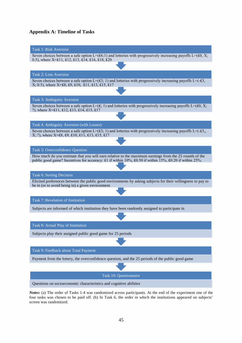
45
Appendix A: Timeline of Tasks
Notes: (a) The order of Tasks 1-4 was randomized across participants. At the end of the experiment one of the four tasks was chosen to be paid off. (b) In Task 6, the order in which the institutions appeared on subjects’ screen was randomized.
Task 10: Questionnaire
Questions on socioeconomic characteristics and cognitive abilities
Task 9: Feedback about Total Payment
Payment from the lottery, the overconfidence question, and the 25 periods of the public good game
Task 8: Actual Play of Institution
Subjects play their assigned public good game for 25 periods
Task 7: Revelation of Institution
Subjects are informed of which institution they have been randomly assigned to participate in
Task 6: Sorting Decision Elicited preferences between the public good environments by asking subjects for their willingness to pay to be in (or to avoid being in) a given environment
Task 5: Overconfidence Question How much do you estimate that you will earn relative to the maximum earnings from the 25 rounds of the public good game? Incentives for accuracy: ₤1 if within 10%, ₤0.50 if within 15%, ₤0.20 if within 25%.
Task 4. Ambiguity Aversion (with Losses) Seven choices between a safe option L=(₤3; 1) and lotteries with progressively increasing payoffs L=(-₤3,, X; ?), where X=₤8, ₤9, ₤10, ₤11, ₤13, ₤15, ₤17
Task 3: Ambiguity Aversion Seven choices between a safe option L=(₤; 1) and lotteries with progressively increasing payoffs L=(₤0, X; ?), where X=₤11, ₤12, ₤13, ₤14, ₤15, ₤17
Task 2: Loss Aversion Seven choices between a safe option L=(₤3; 1) and lotteries with progressively increasing payoffs L=(-₤3, X; 0.5), where X=₤8, ₤9, ₤10, ₤11, ₤13, ₤15, ₤17
Task 1: Risk Aversion Seven choices between a safe option L=(₤6;1) and lotteries with progressively increasing payoffs L=(₤0, X; 0.5), where X=₤11, ₤12, ₤13, ₤14, ₤16, ₤18, ₤20

46
Appendix B: Experimental Instructions
Note: These are the written instructions used in all experimental sessions. The order of tasks
for the preference elicitation in Section A was random for each subject. The order of
institutions was the same for all subjects (as appears in the instructions of Section B).
However, the order in which the institutions appeared on subjects’ screen (see Appendix C
for a screenshot) was randomized.
Instructions – Section A
During this experiment, you will take part in two Sections. You will now undertake Section
A. You will learn about Section B at the beginning of that section, where you will receive
new instructions.
At the beginning of this experiment, everyone will receive a lump-sum payment, which
ensures that you will have positive overall earnings.
Section A involves decision making between two options. In the first option, there will
always be a fixed amount of money, whereas, in the second option, there will be some
randomness involved in determining your payoff.
At the end of Section A, one of your decisions will be randomly chosen and you will receive
the payment according to the resulting outcome from this decision.
Your total earnings from this experiment will consist of your income in Section A and your
income in Section B.

47
Risk:
Loss:

48
Ambiguity:
Ambiguity (with losses):

49
Instructions – Section B
You are now about to take part in Section B of this session. For this Section, you will now
have to choose which of the following institutions described below you want to participate in.
If you read the instructions carefully, you can, depending on the decisions that you and other
participants make, earn a considerable amount of money. It is therefore very important that
you read these instructions with care.
These instructions are solely for your private use. It is prohibited to communicate with the
other participants during the session. If you have any questions, please raise your hand, but
avoid distracting others in the room. We would like to stress to you that your answers are
entirely anonymous.
In this Section, unless otherwise stated, we will not speak in terms of Pounds, but of Money
Units. Your entire earnings will, thus, be calculated in Money Units. At the end of the session
the total amount of Money Units you have earned will be converted to Pounds at the
following rate:
1 Money Unit = 0.01 Pounds
At the end of the session your entire earnings will be paid to you in cash. These earnings will
be added to what you have earned from Section A.
At the beginning of Section B, in each period the participants are divided into groups of four.
You will therefore be in a group with 3 other participants. The composition of the groups
will remain the same throughout this Section. Each institution consists of twenty-five
periods. Below we describe each of the four institutions in detail.
After the twenty-five periods, you will need to answer a short sequence of survey questions.

50
INSTITUTION A
At the beginning of each period each participant receives 20 tokens. We call this his or her
endowment. Your task is to decide how to use your endowment. You have to decide how
many of the 20 tokens you want to contribute to a project and how many of them to keep for
yourself.
Your income therefore consists of two parts:
(1) The tokens which you have kept for yourself (“Income from retained tokens”) whereby 1
token = 1 Money Unit.
(2) The “Income from the project”. This income is calculated as follows:
Your income from the project = 0.4 times the total contributions to the project.
For each token which you keep for yourself you earn an income of 1 Money Unit. For each
token contributed to the project instead, then the total contributions to the project would rise
by one token. Your income from the project would rise by 0.4*1=0.4 Money Units. However
the income of the other group members would also rise by 0.4 Money Units each, so that the
total income of the group from the project would rise by 1.6 Money Units. Your contribution
to the project therefore also raises the income of the other group members. On the other hand
you earn an income for each token contributed by the other members to the project. For each
token contributed by any member you earn 0.4*1=0.4 Money Units.
The income of each group member from the project is calculated in the same way, i.e., each
group member receives the same income from the project. Assume, for example, that the sum
of the contributions of all group members is 40 tokens. In this case each member of the group
receives an income from the project of: 0.4*40 = 16 Money Units.
Your period income is therefore calculated as follows:
Period income in Money Units =
(20 – your contribution to the project) + 0.4*(total contributions to the project)

51
INSTITUTION B
Institution B consists of two stages in each period. The first stage is identical to that of
Institution A. That is, at the first stage you have to decide how many tokens out of 20 you
want to contribute to a project (and hence you decide with it how many tokens you keep for
yourself). Your income from the first stage will be calculated exactly in the same way as in
Institution A. For each token you keep for yourself, you earn an income of 1 Money Unit. For
any token you contribute to the project, you and all other group members will earn 0.4 Money
Units. Therefore, each token that another group member contributes to the project will
increase your income by 0.4 Money Units.
What is different in Institution B?
Now there is a second stage. At the start of the second stage, you see how much each group
member contributed to the project in the first stage. During this stage, you can alter the
income of each other group member by assigning negative points. By assigning negative
points, you can decrease the income of each other group member. You can assign
between 0 and 5 negative points to each group member.
Each negative point that you assign decreases this group member’s income by 3 Money
Units. For example, if you assign 2 negative points, this group member’s income will be
decreased by 6 Money Units. The only exception arises because negative points cannot do
more than eliminate a group member’s first stage income. Thus, a group member’s income
cannot be decreased by more than their first stage income, through negative points assigned
by others.
If you assign negative points, you have costs in Money Units. The more negative points you
assign, the higher your costs. For each negative point that you assign, there is a cost to
you of 1 Money Unit. For example, if you assign 2 negative points, this costs you 2 Money
Units. We refer to this as “Cost of negative points assigned by you”. Just as you can decrease
other members’ income by assigning negative points to them, so they can also decrease your
income by the same method. We refer to this as “Number of negative points assigned to you”.

52
Your period income is therefore calculated as follows:
Period income in Money Units =
= Income from the first stage
– Cost of negative points assigned by you
– 3*(Number of negative points assigned to you)
if the impact of the negative points assigned to you is less than the income from the first
stage;
OR
= 0 – Cost of negative points assigned by you
if the impact of the negative points assigned to you is greater than the income from the first
stage.

53
INSTITUTION C
Institution C consists of two stages in each period. The first stage is identical to that of
Institution A. That is, at the first stage you have to decide how many tokens out of 20 you
want to contribute to a project (and hence you decide with it how many tokens you keep for
yourself). Your income from the first stage will be calculated exactly in the same way as in
Institution A. For each token you keep for yourself, you earn an income of 1 Money Unit. For
any token you contribute to the project, you and all other group members will earn 0.4 Money
Units. Therefore, each token that another group member contributes to the project will
increase your income by 0.4 Money Units.
What is different in Institution C?
Now there is a second stage. At the start of the second stage, you see how much each group
member contributed to the project in the first stage. During this stage, you can alter the
income of each other group member by assigning positive points. By assigning positive
points, you can increase the income of each other group member. You can assign
between 0 and 5 positive points to each group member.
Each positive point that you assign increases this group member’s income by 1 Money
Unit. For example, if you assign 2 positive points, this group member’s income will be
increased by 2 Money Units.
If you assign positive points, you have costs in Money Units. The more positive points you
assign, the higher your costs. For each positive point that you assign, there is a cost to you
of 1 Money Unit. For example, if you assign 2 positive points, this costs you 2 Money Units.
We refer to this as “Cost of positive points assigned by you”. Just as you can increase other
members’ income by assigning positive points to them, so they can also increase your income
by the same method. We refer to this as “Number of positive points assigned to you”.

54
Your period income is therefore calculated as follows:
Period income in Money Units =
= Income from the first stage
– Cost of positive points assigned by you
+ 1*(Number of positive points assigned to you)

55
INSTITUTION D
Institution D consists of two stages in each period. The first stage is identical to that of
Institution A. That is, at the first stage you have to decide how many tokens out of 20 you
want to contribute to a project (and hence you decide with it how many tokens you keep for
yourself). Your income from the first stage will be calculated exactly in the same way as in
Institution A. For each token you keep for yourself, you earn an income of 1 Money Unit. For
any token you contribute to the project, you and all other group members will earn 0.4 Money
Units. Therefore, each token that another group member contributes to the project will
increase your income by 0.4 Money Units.
What is different in Institution D?
Now there is a second stage. At the start of the second stage, you see how much each group
member contributed to the project in the first stage. During this stage, you can alter the
income of each other group member by assigning negative or positive points. By
assigning negative points, you can decrease the income of each other group member. By
assigning positive points, you can increase the income of each other group member.
You can assign between 0 and 5 negative or positive points to each group member.
Each negative point that you assign decreases this group member’s income by 3 Money
Units. For example, if you assign 2 negative points, this group member’s income will be
decreased by 6 Money Units. The only exception arises because negative points cannot do
more than eliminate a group member’s first stage income. Thus, a group member’s income
cannot be decreased by more than their first stage income, through negative points assigned
by others. Each positive point that you assign increases this group member’s income by
1 Money Unit. For example, if you assign 2 positive points, this group member’s income will
be increased by 2 Money Units.
If you assign either negative or positive points, you have costs in Money Units. The more
negative or positive points you assign, the higher your costs. For each negative point that

56
you assign, there is a cost to you of 1 Money Unit. For each positive point that you
assign, there is a cost to you of 1 Money Unit. For example, if you assign 2 negative points,
this costs you 2 Money Units. If you assign 2 positive points, this costs you 2 Money Units.
We refer to this as “Cost of negative points assigned by you” and “Cost of positive points
assigned by you”, respectively.
Just as you can decrease or increase other members’ income by assigning negative or positive
points to them, so they can also decrease or increase your income by the same method. We
refer to this as “Number of negative points assigned to you” and “Number of positive points
assigned to you”, respectively.
Your period income is therefore calculated as follows:
Period income in Money Units = = Income from the first stage
– Cost of negative points assigned by you
– Cost of positive points assigned by you
– 3*(Number of negative points assigned to you)
+ 1*(Number of positive points assigned to you)
if the impact of the negative and positive points assigned to you is less than the income from
the first stage;
OR
= 0 – Cost of negative points assigned by you
– Cost of positive points assigned by you
if the impact of the negative and positive points assigned to you is greater than the income
from the first stage.
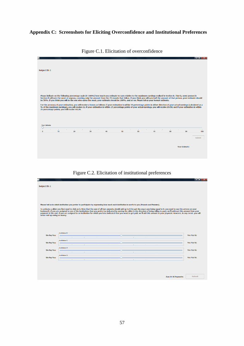
57
Appendix C: Screenshots for Eliciting Overconfidence and Institutional Preferences
Figure C.1. Elicitation of overconfidence
Figure C.2. Elicitation of institutional preferences

58
Appendix D: Additional Statistical and Regression Analysis
Table D.1. Means and Standard Deviations of Preference Measures
(Excluding the 40 “Switchers”)
Preference measure Mean Standard deviation
Risk aversion 3.47 1.70
Loss aversion 2.98 2.04
Ambiguity aversion (without losses) 4.36 1.83
Ambiguity aversion (with losses) 3.62 2.36
Table D.2. Pair-wise Correlation Coefficients of Preference Measures
(Excluding the 40 “Switchers”)
Risk Loss Ambiguity without loss
Ambiguity with loss
Risk 1
Loss .33*** [.00] 1
Ambiguity without loss
0.44*** [.00]
0.07 [.36] 1
Ambiguity with loss
0.20** [.01]
0.64*** [.00]
0.24*** [.00] 1

59
Table D.3. Preference Measures and Choice of Institutions (Excluding the 40 “Switchers”)
Note: OLS regressions with robust standard errors in square brackets. * denotes significance at the 10-percent level, ** denotes significance at the 5-percent level, and *** denotes significance at the 1-percent level.
Table D.4. Assignment of Points for Different Levels of Deviation Across All Periods
Treatments [–20, –11] [–10, –1] 0 [1, 10] [11, 20] VCM with punishment –2.21 –0.87 –0.08 –0.33 –0.35 VCM with reward 0.01 0.10 0.13 0.43 0.63 VCM with punishment and reward –2.00 –0.41 –0.01 0.01 –0.04
Dependent variable: ranking of each institution (1, 1.5, ..., 4) VCM rank VCM with
punishment rank
VCM with reward rank
VCM with punishment and
reward rank 1 2 3 4 5 6 7 8 Std. Risk Aversion
–23.96 (22.52)
–26.19 (23.19)
5.67 (21.97)
5.45 (21.20)
4.66 (18.59)
4.13 (17.03)
13.64 (20.08)
16.61 (20.78)
Std. Loss Aversion
25.02 (25.85)
18.23 (26.34)
22.28 (29.59)
22.80 (31.03)
–22.97 (24.54)
–23.70 (24.70)
–24.33 (25.19)
–17.34 (25.57)
Std. Ambiguity Aversion
15.81 (20.10)
19.00 (22.24)
–6.93 (22.31)
0.96 (23.97)
–10.00 (21.63)
–16.39 (22.47)
1.12 (19.75)
–3.58 (21.34)
Std. Ambiguity (with loss) Aversion
-45.71* (25.10)
–39.43 (25.25)
–3.28 (27.52)
–0.32 (28.62)
15.46 (24.31)
12.90 (24.57)
33.53 (25.50)
26.84 (26.43)
Over- confidence 4.06
(104.37) 88.44 (117.66) –42.57
(100.81) –49.93 (93.22)
Correct CRT questions –2.33
(19.94) –35.97 (19.45) 34.28**
(16.91) 4.01 (16.30)
Male –25.76 (41.47) 15.48
(47.79) –40.04 (39.45) 50.32
(37.60)
Age –3.72 (5.29) 8.92*
(5.20) –8.59* (4.62) 3.39
(4.38)
UK 71.38 (43.52) –3.304
(48.96) 12.91 (44.66) –80.99*
(42.37)
Constant 26.61 (18.70)
84.08 (133.53)
–27.21 (19.53)
–217.06 (143.53)
–10.01 (17.81)
154.57 (133.50)
10.62 (17.18)
–21.60 (123.11)
Obs. 152 152 152 152 152 152 152 152