IEEE TRANSACTIONS ON MAGNETICS, VOL. 42, NO. 4, APRIL 2006 1227

Selection of Approximation Models forElectromagnetic Device Optimization

Linda Wang and David A. Lowther

Department of Electrical and Computer Engineering, McGill University, Montreal, QC H3A 2A7, Canada

Approximation models are frequently used in design optimization in order to reduce computational cost. Many new forms of approx-imation model have appeared recently, but it is difficult to know which one to choose for the problem at hand. This paper investigatesa model selection strategy that estimates the accuracy of all the different approximation models under consideration, so that the mostaccurate one can be chosen.

Index Terms—Approximation models, cross-validation, electromagnetic devices, numerical analysis.

I. INTRODUCTION

THE optimization of electromagnetic devices is often per-formed using finite-element analysis code coupled with

optimization algorithms. In order to reduce the computationalcost of finite-element analysis, simple approximation models ofthe device performance can be built based on several test runsof the analysis code. These models can then be used in placeof finite-element analysis during optimization. This practice iscommonly used in engineering design where a single run of theanalysis code is very expensive [1].

Traditionally, the most common type of approximationmodels is low-order polynomials. However, many new typesof models have emerged recently that claim to have moreflexibility in modeling nonlinearities. Given this variety ofchoices, it has become difficult for an engineer to select themost appropriate model for the device under study. The goal ofour work is to investigate a model selection strategy that canchoose the most accurate model out of a given set of differentmodel types. We demonstrate that the cross-validation methodused for assessing a model’s accuracy can give a reliable metricfor model selection.

II. BACKGROUND

All approximation models are constructed with three steps:1) select a set of sample points in the design space; 2) run theanalysis code at each sample point and obtain the correspondingresponse data; and 3) fit the response data to a model. In orderto select the most appropriate model for the problem at hand,we analyze the response data obtained in Step 2 and predictthe accuracy of all the model types under consideration. Thefollowing sections briefly describe three approximation modeltypes considered in this work, and also discuss the cross-valida-tion method which can be used to assess their accuracy.

Digital Object Identifier 10.1109/TMAG.2006.871954

A. Response Surface Modeling

Response surface (RS) models fit the response data to alow-order polynomial using least-squares regression. Quadraticpolynomials are most commonly used, which have the form

where is the number of design variables, is a vector of lengthcontaining the design variable values, and the s are model

parameters determined with least-squares regression. RS mod-eling smooths out data rather than interpolating them. Due totheir ease of use, RS models are the most popular model typefound in the optimization of electromagnetic devices [2], [3].

B. Radial Basis Functions

Radial basis function (RBF) models use a linear combina-tion of radially symmetric functions to interpolate sampled datapoints. The simplest form of these models is

where is the Euclidean distance, is the total number ofsample points, is the th sample point, and the s are modelparameters found by solving a linear system of equations.RBF models are shown to produce good fit for arbitrary contours[4].

C. Kriging

The most common form of Kriging models consist of a con-stant term plus a departure

(3)

where the departure is a realization of a stochastic processwith mean zero, variance , and nonzero covariance [5]. In thismodel, can be thought of as a “global” approximation for theentire design space, while is added to create “localized”deviations so that the model can interpolate sampled data points.

0018-9464/$20.00 © 2006 IEEE

1228 IEEE TRANSACTIONS ON MAGNETICS, VOL. 42, NO. 4, APRIL 2006

The covariance matrix of is

(4)

where is the correlation matrix, and is the user-specifiedcorrelation function. Gaussian correlation functions are mostcommonly used. They have the form

(5)

Fitting an approximation model then consists of estimating theunknown parameters in (3), in (5), and (the varianceof ). and are found using maximum likelihood es-timation, while is solved as an -dimensional optimizationproblem. Kriging claims to be superior in modeling local non-linearities. However, it is also significantly more complex thanRS and RBF models. Both Kriging and RBF models have beenapplied to the optimization of electromagnetic devices [6].

D. Model Accuracy Assessment and Cross-Validation

It is essential to assess the accuracy of an approximationmodel before it can be used for optimization. Model accuracyis usually assessed by comparing some response data producedby the analysis code with the corresponding response datapredicted by the model. A metric is calculated based on thesetwo sets of values (such as root mean squared error) to quantifythe degree of accuracy.

After a model is built, a straightforward way to assess its ac-curacy is to run the analysis code at a large additional set ofsample points and compare the outputs with the ones predictedby the model. However, this comes at a high cost since runninganalysis code is time-consuming. Cross-validation is a modelassessment method that can estimate the accuracy of a modelwithout requiring any additional sample points. Suppose thatan approximation model has been built using sample pointsand their corresponding response data. A practical version ofcross-validation that can be used to validate this model is as fol-lows [7].

1) Randomly divide the sample points into two mutually-exclusive sets: set with points, and set withpoints.

2) Build a new approximation model using only the samplepoints in and their response data.

3) With this new approximation model, predict the responseat each sample point in . Using these predicted re-sponses along with the true responses already available,calculating a model accuracy metric.

4) Repeat Steps 1)–3) for a total of times, and calculatethe average of the accuracy metric found in Step 3) acrossthese iterations. This average is then cross-validation’sestimate of the model accuracy.

Cross-validation essentially works by estimating a model ac-curacy metric with only a limited number of sample points. Themodel accuracy metric obtained this way cannot be as reliable asone calculated using a large number of additional sample points.However, this method saves significant computation time since

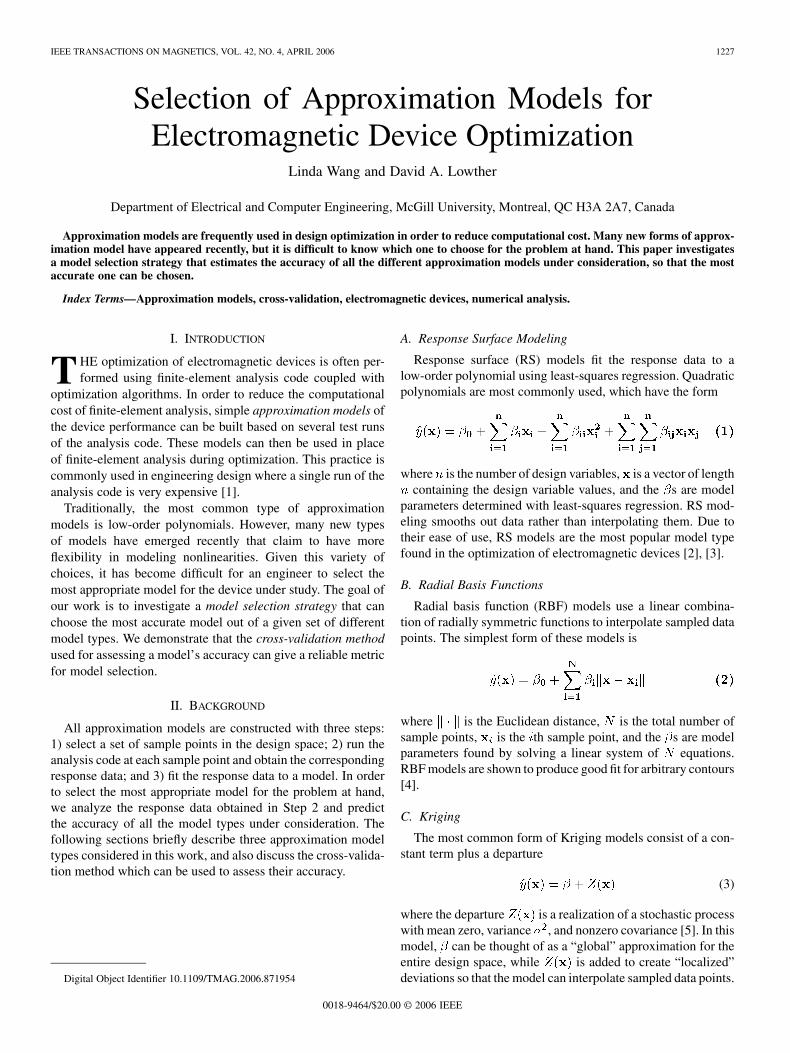
Fig. 1. 1–D and 2–D mathematical test functions.

it avoids running the analysis code. A recommended value forin the method was found to be [7].

III. MODEL SELECTION USING CROSS-VALIDATION

Given several different types of approximation models, cross-validation can be used to select the one with the best accuracymetric value. This model selection strategy requires generatingand cross-validating all the approximation models under con-sideration. The computational cost of this approach is justifiedby the fact that model fitting and assessment usually take onlyseconds, while a single run of the analysis code could last min-utes to hours, if not longer.

IV. EXPERIMENTAL SETUP

This work investigates the reliability of using cross-validationto select the best model out of RS, RBF, and Kriging models. Wetest the model selection method on both mathematical functionsand electromagnetic applications.

A. Mathematical Test Functions

The eight mathematical functions used in this work areshown in Fig. 1. These are smooth, nonlinear functions com-monly used for testing optimization algorithms [8]. Functions

– are one-dimensional (1-D) problems, while – aretwo-dimensional (2-D) problems. We will sample and buildapproximation models for these functions.

B. Electromagnetic Applications

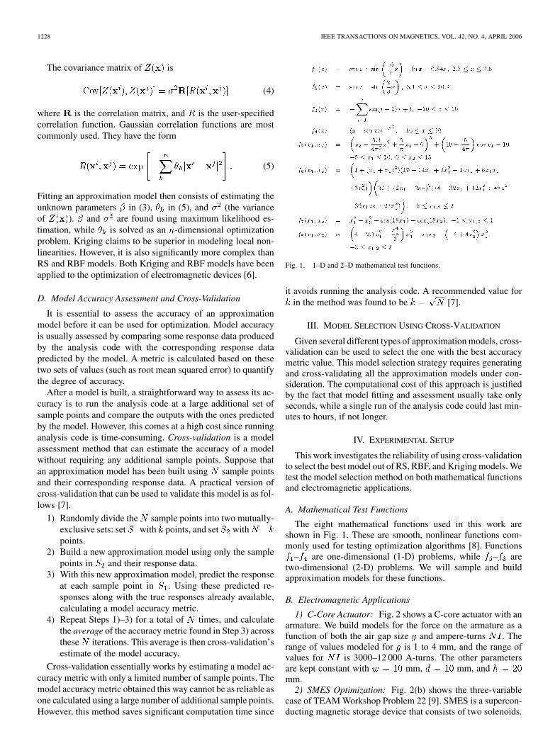
1) C-Core Actuator: Fig. 2 shows a C-core actuator with anarmature. We build models for the force on the armature as afunction of both the air gap size and ampere-turns . Therange of values modeled for is 1 to 4 mm, and the range ofvalues for is 3000–12 000 A-turns. The other parametersare kept constant with mm, mm, andmm.

2) SMES Optimization: Fig. 2(b) shows the three-variablecase of TEAM Workshop Problem 22 [9]. SMES is a supercon-ducting magnetic storage device that consists of two solenoids.

WANG AND LOWTHER: SELECTION OF APPROXIMATION MODELS FOR ELECTROMAGNETIC DEVICE OPTIMIZATION 1229

Fig. 2. Two test problems. (a) C-core actuator with armature. (b) SMES (from[9]).

The dimensions of the inner solenoid stay fixed, while the di-mensions of the outer solenoid (determined by variables ,and ) should be optimized to reduce stray fields while keepingthe stored energy close to 180 MJ. The stray field is evaluatedalong 22 equidistant points on lines a and b. The following ob-jective function is to be minimized:

Energy(6)

where

In this work, approximation models are built for the objectivefunction. Both the SMES and the C-core problem use MagNet[10] as the analysis program.

C. Sampling Strategy

To select the set of sample points with which to build anapproximation model, we use Latin hypercube sampling. Thisstrategy samples all regions of the design space equally, makingit especially suitable for modeling with computer analysis code[5]. For the mathematical functions, we tested 15 different sizesof that varied from 8 to 64. For the C-core problem, we usedtwo different sizes of 8 and 16. For the SMES problem, we usedtwo different sizes of 16 and 64.

D. Model Accuracy Metrics

Many types of metrics can be used to assess model accuracy.Since we use cross-validation’s estimation of such metrics toselect models, it is important to examine whether the model se-lection is affected by the type of metric used. We examine twopopular metrics, root mean squared error (RMSE) and R squared

. They are defined as follows:

(7)

(8)

where is the number of responses used to calculate the metric,is the th response produced by analysis code, is the cor-

responding th prediction produced by the model, and is the

mean of the ’s. An accurate model should have a low RMSEvalue or a high value.

E. Verification of Model Selection

In order to verify the accuracy of model selection done bycross-validation, we use 2000 additional sample points for alltest problems. The accuracy metrics are calculated using these2000 points. We can then find the error in cross-validation’sestimation of the metrics, and also determine whether the modelselected is indeed the most accurate one (i.e., the one with thebest metric value as calculated using the 2000 points).

In order to have fair comparison among the problems, nor-malization is done so that the metrics produced are between zeroand one. The error in estimating a metric is then

error metric metric

where metric is the metric value estimated using cross-valida-tion, and metric is the metric calculated using 2000 points.The error is between zero and one.

V. RESULTS

A. Mathematical Functions

1) Error in Metric Estimation: Fig. 3(a) shows the averageerror in estimating the RMSE for the four 1-D mathematicalfunctions. The number of sample points is varied from 8 to 64,and the average error is shown separately for the three types ofmodels investigated. Linear fits for the average errors are alsoshown. We can see that the estimation error of the RMSE de-creases for all three models as the number of sample pointsincreases. This agrees with the intuition that cross-validationshould become more reliable as the number of sample pointsincreases. For these 1-D problems, the estimation error for theRMSE is quite low (less than 0.3) when the number of samplesreaches 24. The difference in the estimation error among thethree models does not appear to be significant; therefore, the re-liability of cross-validation with RMSE is not dependent uponthe model type.

Fig. 3(b) shows the average error in estimating for the four1-D mathematical functions. Cross-validation performs signif-icantly worse for RS models than the other two models whenestimating . Kriging and RBF, on the other hand, had similarresults to the ones for RMSE.

Fig. 4(a) and (b) shows the RMSE and estimation error forthe four 2-D problems. These figures indicate similar trends tothe ones discussed for 1-D problems. As before, cross-validationperforms worse for RS models when it estimates .

2) Accuracy of Model Selection: Fig. 5 shows the per-centage of time that cross-validation selected the correct modelfor the eight mathematical functions. As the number of samplepoints increased, cross-vailidation becomes more reliable,resulting in a higher accuracy of model selection. In fact, whenthe number of sample points is large, incorrect model selectionsare largely due to two models having very similar accuracies,making them difficult to distinguish with cross-validation.

The results also show that cross-validation with hasa lower model selection accuracy than cross-validation withRMSE. This is possibly due to the high estimation errors forRS models. Although not shown, it is interesting to note that inover 80% of the cases tested, the functions were modeled best

1230 IEEE TRANSACTIONS ON MAGNETICS, VOL. 42, NO. 4, APRIL 2006

Fig. 3. Average error in metric estimation for 1-D functions. (a) RMSEestimation. (b) R estimation.

Fig. 4. Average error in metric estimation for 2-D functions. (a) RMSEestimation. (b) R estimation.

with Kriging. This verifies Kriging’s claim to be a very flexiblefor highly nonlinear functions.

B. Electromagnetic Applications

The C-core problem was modeled with sample sizes of 8 and16. Model selection was correct for all cases, both when cross-

Fig. 5. Percentage of correct model selections.

validation was performed with RMSE and . In all cases, thebest model was the RS model, indicating that this problem isquadratic.

The SMES objective function was modeled with sample sizesof 16 and 64. Model selection was also correct for all cases. Witha sample size of 16, RS models were the best; with a sample sizeof 64, Kriging models were the best (while RS models were justslightly worse). This indicates that the SMES objective functionis highly quadratic in its variables as well.

VI. CONCLUSION

We have shown that using cross-validation is a feasiblestrategy for the selection of approximation models. Resultsshow that using RMSE as the model accuracy metric is morereliable than using . Furthermore, the performance ofcross-validation using RMSE is not biased against any modeltype tested, whereas cross-validation using does not performas well for RS models. For highly nonlinear 1-D problems,around 16 samples were needed for the model selection to bereliable; for highly nonlinear 2-D problems, around 32 sampleswere needed.

REFERENCES

[1] T. W. Simpson et al., “Approximation methods in multidisciplinary anal-ysis and optimization: A panel discussion,” Struct. Multidisc. Optim.,vol. 27, pp. 302–313, 2004.

[2] D. Dyck, D. A. Lowther, Z. Malik, R. Spence, and J. Nelder, “Responsesurface models of electromagnetic devices and their application to de-sign,” IEEE Trans. Magn., vol. 34, no. 3, pp. 1821–1824, May 1999.

[3] J. T. Li, Z. J. Liu, M. A. Jabbar, and X. K. Gao, “Design optimizationof cogging torque minimization using response surface methodology,”IEEE Trans. Magn., vol. 40, no. 2, pp. 1178–1179, Mar. 2004.

[4] M. J. D. Powell, “Radial basis functions for multivariable interpolation:A review,” in Algorithms for Approximation. Oxford, U.K.: OxfordUniv. Press, 1987, pp. 105–210.

[5] T. J. Santner, B. J. Williams, and W. I. Notz, The Design and Analysisof Computer Experiments. New York: Springer-Verlag, 2003.

[6] L. Lebensztajn, C. A. R. Marretto, M. C. Costa, and J.-L. Coulomb,“Kriging: A useful tool for electromagnetic devices optimization,” IEEETrans. Magn., vol. 40, no. 2, pp. 1196–1199, Mar. 2004.

[7] M. Meckesheimer and A. J. Booker, “Computationally inexpensivemetamodel assessment strategies,” AIAA J., vol. 40, no. 10, pp.2053–2060, 2002.

[8] A. Törn and A. Zilinskas, Global Optimization. New York: Springer-Verlag, 1989.

[9] B. Brandstaetter. SMES Optimization Benchmark, TEAM Work-shop Problem 22, 3 Parameter Problem. [Online]. Available:http://www-igte.tugraz.ac.at/archive/team/index.htm

[10] MagNet 6 User Manual, 2004. Infolytica Corp.

Manuscript received June 20, 2005 (e-mail: linda.wang@mail.mcgill.ca).