Selling to Strategic Consumers When Product Value is Uncertain:The Value of Matching Supply and Demand

Robert SwinneyGraduate School of Business, Stanford University

518 Memorial Way, Stanford, CA 94305-5015, swinney@stanford.edu

May, 2008

Abstract

Quick response inventory practices�which combine reduced production leadtimes, sophisti-cated information systems, and continuous demand forecasting improvement�are often discussedas a potential remedy to the negative aspects of supply and demand mismatches. We addressthe value of these practices when selling to a forward-looking consumer population with uncer-tain, heterogeneous values for a product. Consumers have the option of purchasing the productearly, before its value has been learned, or delaying the purchase decision until a time at whichvaluation uncertainty has been resolved, a trade-o¤ frequently made by consumers shopping fornew or innovative products. While individual consumer valuations are uncertain ex ante, themarket size is uncertain to the �rm. The �rm may either commit to a single production run ata low unit cost prior to learning demand, or commit to a quick response strategy which allowsadditional production (at a higher unit cost) after learning additional demand information. We�nd that it is possible for a quick response strategy to decrease the pro�t of the �rm, thoughwhether this occurs depends on various characteristics of the market; speci�cally, we identifyconditions under which quick response always increases pro�ts (when prices are increasing, whendissatis�ed consumers can return the product) and conditions under which quick response maydecrease pro�ts (when prices are constant or when consumer returns are not allowed). Finally,we demonstrate that our model is also applicable to a manufacturer selling to a population ofstrategic retailers, and we discuss factors that in�uence the manufacturer�s incentives to adopta short leadtime manufacturing strategy.

1 Introduction

In October of 2007, Susan faced a dilemma. Her three year-old son, Ryan, had recently developed

a strong interest in the Little Einstein line of toys produced by Fisher-Price. Susan knew that

one particular toy�the Pat-Pat Rocket�was rumored to be a �hot toy�for toddlers during the 2007

holiday shopping season. By chance, Susan one day came across a store with several Pat-Pat

Rockets in stock. She knew that if she purchased the toy immediately, there was no guarantee

that Ryan would still enjoy Little Einstein products in three months time; his taste in toys seemed

to change weekly. If she did not buy the toy now, however, she believed her chances of �nding it in

1

the future may be slim, particularly if the toy turned out to be a hot holiday gift. Susan ultimately

chose to purchase the Pat-Pat Rocket; the risk of not obtaining the toy was too great to delay her

decision until closer to the holidays.

Parents increasingly participate in this unfortunate holiday ritual (Slatalla 2002), trading o¤

the risk of buying early and facing uncertain value for the product (i.e., possibly buying a toy

that turns out to be a �dud� or that their child does not want) with the risk of buying late

and facing uncertain availability for the product (i.e., experiencing a stock-out). Recent history

provides numerous examples of hot holiday toys for which demand outstrips expectations, from

Barbie to Elmo to the Nintendo Wii video game system. Stock-outs during the holidays are

assumed to be particularly costly to �rms, as consumers shopping for gifts are more likely to switch

to a competitor�s product rather than wait for an inventory replenishment that occurs after the

holidays have concluded. Indeed, the perception is that potential losses due to inventory shortages

during the holidays can be enormous�Richtel (2007), for example, reports estimates that Nintendo

experienced lost sales in excess of $1 billion due to unsatis�ed demand on the Wii video game

system during the 2007 holiday season.

Long production and shipping leadtimes are often cited as key causes for holiday gift shortages,

particularly on those products manufactured in Asia and exported to the US or Europe. Due to

these long leadtimes, demand forecasts must be made far in advance of the selling season, when

uncertainty concerning �nal demand is high. Thus, if leadtimes could be reduced�via, for example,

localized production, increased capacity, improved information systems, and expedited shipping

methods�allowing for a rapid response to updated demand information closer to (or during) the

selling season, supply and demand could be more closely matched, reducing or eliminating costly

shortages. Such techniques (often known as reactive capacity or quick response systems) can be

expensive due to expedited production or transportation costs, but are known to provide signi�cant

value to �rms by better matching supply with uncertain demand (Fisher and Raman 1996). The

consensus is that quick response systems are bene�cial to a �rm: indeed, in the absence of �xed

costs related to the implementation of such systems, the opportunity to procure additional inventory

after learning updated demand information is an option which always possesses positive value.

In this paper, we consider whether (and under what conditions) quick response inventory prac-

tices do in fact bene�t a �rm. Motivated by our example of holiday gifts, we consider a product

2

characterized by initially uncertain consumer value. This may be the case if, for instance, the

product is a new or innovative item (e.g., a complex or innovative product such as a Nintendo Wii,

an Apple iPhone, or an automobile), a media item (such as books, movies, music, or video games),

or the consumer�s requirements for the item are uncertain (e.g., snow skis for a potential weekend

trip in two months when weather is unknown, or a gift for a child whose preferences frequently

change). Over time, consumers learn more information about the product and gain a better sense

of its value; for example, via channels such as professional product reviews from web sites and

magazines, the reviews of fellow consumers (e.g., from online retailers such as Amazon.com), the

experiences of friends and family who may have purchased the same product, or via the resolution

of intrinsic uncertainty in product value (e.g., the weather a¤ecting the value of a pair of skis is

known the day of the ski trip). Individual consumers thus makes a decision on when and whether

to purchase the product: the later the customer waits to buy, the more information she will have

about product value and the greater the risk of a stock-out.

When consumers experience this type of time dependent learning, greater availability resulting

from an improved matching of supply and demand encourages consumers to delay purchasing the

product: by reducing the likelihood of a stock-out, the �rm decreases the riskiness of waiting

to learn more information about product value. Thus, there is a clear interaction of consumer

learning (of product value) and �rm learning (of product demand). We explore this interaction

by addressing how the responsiveness of the �rm�s supply chain�its ability to respond to improved

demand information�a¤ects consumer purchasing behavior. We analyze models with a single �rm

selling to a rational, forward-looking consumer population. Consumers choose to either purchase

early�prior to learning their value for a product�or purchase late, after learning their value. The

�rm chooses to either commit to a single production run in advance of learning product popularity

or to adopt the ability to rapidly produce inventory after stochastic demand is revealed.

Using this stylized framework, we demonstrate that the basic intuition that quick response

provides an option with purely positive value may be incorrect; that is, even without �xed costs it

is possible for a �rm to be worse o¤ if it has an additional procurement opportunity after receiving

updated demand information. This occurs when consumers�cognizant of the results of the �rm�s

operating policies, in particular the inventory availability�modify their own purchasing behavior to

account for the implementation of a quick response system. In other words, while quick response

3

does better match supply and demand, demand itself can be negatively a¤ected once consumers

become aware of the increased availability resulting from quick response and optimize their own

behavior accordingly. The net e¤ect may decrease �rm pro�ts, though we demonstrate that

whether this occurs (and to what degree it occurs) depends heavily on several characteristics of the

selling environment; speci�cally, when prices increase over time or when dissatis�ed consumers can

return the product for a full refund, quick response always increases �rm pro�t, whereas if prices

are constant or decline over time or if consumers cannot return the product for a full refund, quick

response may decrease �rm pro�t. Finally, we demonstrate that our model of a �rm selling to

multiple consumers with uncertain value is analogous to a manufacturer selling to multiple retailers

facing uncertain demand, and we derive additional insights concerning this interpretation of the

model.

The remainder of the paper is organized as follows. §2 provides a review of the literature. §3

introduces the model, and §§4�5 analyze the consumer decision and the equilibrium to the game,

respectively. Three extensions are then analyzed: consumer returns in §6, pricing in §7, and a

model of a manufacturer selling to multiple retailers in §8. §9 concludes the paper with a discussion

of the results.

2 Related Literature

There are two areas of the literature that are of particular relation to this analysis: the �rst

concerns forward-looking or �strategic�consumer behavior. Explicitly modeling the intertemporal

purchasing decision of rational consumers has received increased attention in recent years; see, for

example, Aviv and Pazgal (2007), Liu and van Ryzin (2005), Su and Zhang (2005), and Jerath et al.

(2007). The most relevant papers to our own from this stream of research are those addressing

uncertain consumer valuations. DeGraba (1995) explains why a �rm may intentionally understock

to induce consumers to purchase when valuations are uncertain and learned over time. Unlike

our model, there is no demand uncertainty to the �rm. Xie and Shugan (2001) demonstrate

that selling to consumers prior to the determination of value and consumption (e.g., with advance

ticket sales) can substantially increase �rm pro�ts. Alexandrov and Lariviere (2006) consider the

problem of a restaurant choosing whether to o¤er reservations (guaranteed seats) to customers who

4

may or may not value dining on a given night, demonstrating when reservations increase the pro�t

of the �rm. Dana (1998) and Akan et al. (2007) discuss optimal pricing to screen heterogeneous

consumers whose values are revealed over time. In these papers, in contrast to our model, inventory

(or capacity) is either in�nite, exogenously set, or �xed throughout the selling season, and hence

issues of inventory replenishment after receiving updated demand information are not considered.

An exception is Debo and van Ryzin (2007), who consider a periodic review inventory problem.

However, in their model the base-stock level is exogenously given, as is the decision of how often to

replenish, whereas in our model, inventory levels and the decision of whether to obtain a midseason

replenishment are endogenously determined.

Uncertain consumer valuations are also a hallmark of the herding literature�see, e.g., Bikhchan-

dani et al. (1992). Typically in this literature, the actions of the �rm are �xed, while consumers

observe the sequence of sales and use Bayesian updating to determine whether to purchase a prod-

uct with uncertain value. An exception is Debo (2007), which incorporates both the consumer

learning characteristics of the herding literature and the �rm�s decision to price optimally with �xed

inventories. In contrast to the herding literature, our model does not allow consumers to observe

the sequence of sales of the product and infer value from this information; rather, valuations are

exogenously revealed over time, e.g., via external channels such as expert product reviews. We

abstract from the consumer learning dynamics of the herding literature to focus instead on the

inventory game between the �rm and consumers, as well as the decision to adopt quick response

inventory practices.

In §6, we address consumer returns policies which allow customers who buy prior to learning

their value to return the product should their realized valuation turn out to be low. Such policies

have received attention in the literature: Davis et al. (1995) and Moorthy and Srinivasan (1995)

analyze the value of money-back guarantees when selling to consumers with uncertain value; Gallego

and Sahin (2006) discuss multiperiod pricing of a single-consumption good with �xed capacity and

unknown value to consumers, and demonstrate that selling call options on capacity can increase

�rm revenue (call options being analogous to costly product returns); Su (2007) provides an analysis

of how consumer product returns a¤ect inventory decisions when valuations are learned after the

purchase of an item (e.g., experience goods); and Coughlan et al. (2007) address the role of returns

policies in competitive retail settings. These papers do not consider the impact of consumer returns

5

policies on a �rm�s incentives to adopt a rapid procurement strategy, however.

The second broad stream of research related to our own is the quick response literature�see,

for example, Fisher and Raman (1996), Eppen and Iyer (1997), Iyer and Bergen (1997), and

Fisher et al. (2001). In the absence of strategic consumer behavior, these papers demonstrate the

value engendered by the ability of a �rm to react quickly to updated demand information. In a

related paper (Cachon and Swinney 2007), we address the value of quick response systems in a

fashion retail setting with forward-looking consumers. The model in Cachon and Swinney (2007)

is characterized by markdowns and known consumer valuations, and consumers may strategically

delay purchasing in order to �get a good deal�when the item goes on sale. The present model,

by contrast, is characterized by constant (or increasing, as discussed in §7) prices and unknown

consumer valuations�as a result, consumers delay purchasing to obtain better information about

product value. Consequently, while Cachon and Swinney (2007) is applicable to setting in which

value is easily judged and markdowns are likely (e.g., fashion), the present analysis is applicable to

more complex products in which value is di¢ cult to judge or inherently stochastic.

3 Model

A single �rm sells a single product at an exogenous price1 p to a consumer population of uncertain

size, N . Uncertainty in market size is the result of an exogenous stochastic process; that is, N is a

random variable with positive support, distribution function F (�) and density f (�). The product

is sold over two periods. At the start of the �rst period, neither the �rm nor consumers know the

value of N . At some point in the �rst period (e.g., after observing early sales), the �rm exogenously

and perfectly learns N .2

In addition to market size uncertainty, consumers face uncertainty about their own private

valuations for the product. Nature moves �rst (prior to the start of the game) and decides the

�type�of each consumer: a fraction � of the population has positive value v > p for the item, while

a fraction 1� � has zero value. If a consumer possesses value v for the product, we refer to her as1 In §7, we relax the assumption of exogenous prices and consider endogenous pricing.2 In reality, forecast updating and re�nement may be the the result of an endogenous process, e.g., monitoring

early sales and imputing total demand, or performing market research. To avoid issues outside the scope of thisanalysis�e.g., demand estimation based on stochastic arrivals�we assume that the revelation of N is exogenous andperfect.

6

a �high type�consumer, whereas if she possesses zero value for the product, we refer to her as a

�low type�consumer.

In the �rst period, consumers do not know their private valuation for the product (their type).

In the second period, consumers exogenously learn their value for the product (e.g., via product

reviews from professionals and other consumers, experiences with demonstration units in-store,

etc.). While consumers do not know their individual valuations in period one, they do know the

underlying probability structure that determines their type (i.e., they know �); given this structure,

from the point of view of an individual consumer (absent any additional information), the consumer

is high type with probability � and low type with probability 1� �.

In the �rst period, each consumer receives a noisy private signal that is an indication of her

type. We de�ne � to be the quality of the signal, i.e., the probability that the signal is correct.

For example, a high type consumer receives a signal of high product value with probability �, and

a low type consumer receives a signal of low product value with the same probability. We allow

consumers to be heterogeneous in the quality of their private signals by letting � be distributed

among the population (independently of consumer type) according to the continuous distribution

G (�) with support on the interval (1=2; 1). Such heterogeneity in the quality of the signal may

represent, for example, domain expertise of the population in the product category (e.g., some

consumers are highly technical and capable of accurately judging the quality of a new, high tech

product, while some less sophisticated consumers receive more noisy signals that leave them less

sure of product value). Consumers are aware of their individual values of �, and the distribution

G (�) and density g (�) of consumer signal strengths is known to the �rm.

After receiving their private signals, consumers arrive at the �rm throughout the �rst period.

Each consumer updates her beliefs of product value (via Bayes�rule) and calculates the expected

utility of purchasing early (before knowing product value) and the expected utility of purchasing

late (after learning product value), based on her private signal and individual signal strength. In

order to evaluate the expected surplus of delaying a purchase until the late period, consumers must

also form expectations on the probability that a unit will be obtained in the late period (i.e., the

second period availability), which we denote b�.Consumers are risk-neutral expected utility maximizers that discount future consumption at

rate � 2 [0; 1], and hence consumers choose to purchase in the period that maximizes their total

7

Period 1 Period 2

The firmproduces initial

inventory.

Consumers arrive, receive a privatesignal of product value, and chooseto either purchase immediately or

wait until period 2.

If firm has QR capabilities, market size(N) is learned. A second productionrun occurs and arrives immediately.

Consumers who voluntarily waitedfor period 2 arrive and purchase ifthey have positive value and the

product is available.

Valuations revealedto consumers.

Before the Selling Season

Figure 1. Sequence of events.

expected discounted surplus (expected product value minus purchase price). All consumers who

arrive at the store in the second period know their value and purchase if and only if they have

positive surplus and the product is in-stock, and any consumer who does not obtain a unit receives

zero surplus.

We consider two potential operating regimes for the �rm: the single procurement regime (SP),

and the quick response regime (QR). In the single procurement regime, all production occurs in

advance of the selling season, and the �rm chooses an inventory level q before learning market size

(N). There is a linear unit production or ordering cost c1. In the quick response regime, the

�rm is allowed to procure some inventory q prior to the realization of N , but may also produce

or procure additional inventory�at an increased cost�after monitoring initial sales and updating

demand forecasts in the �rst period. Inventory procured using quick response is assumed to arrive

immediately and prior to any stock-out in period one. In this regime, the unit procurement

cost prior to the realization of N is c1, and the unit procurement cost after N has been realized

is c2, where c1 � c2. The �rm is assumed to have in�nite reactive capacity, though capacity

constraints may easily be added without qualitatively a¤ecting any results. The �rm chooses an

initial inventory level q at the start of the game that maximizes total expected pro�t over both

periods, and chooses an inventory replenishment (in the quick response regime) which maximizes

pro�t-to-go. Excess inventory is costlessly carried from period one to period two, and we assume

that excess inventory remaining at the end of period two has zero value. The sequence of events

is summarized in Figure 1.

8

4 The Consumer Decision: Wait or Buy

In this section we analyze the consumer decision: whether to wait or buy. We begin by discussing

the nature of consumer expectations of second period availability (b�). We assume that consumersform rational expectations (see, e.g., Muth 1961, Su and Zhang 2005, and Cachon and Swinney

2007) concerning the availability of the product (i.e., consumers possess beliefs about the chance of

obtaining the product period two that are consistent with the equilibrium availability in the second

period). Rational expectations may be formed by repeated interaction with a �rm over time; for

instance, consumers have come to expect that video game manufacturer Nintendo is incapable of

rapid inventory replenishment to meet demand (Richtel 2007) and hence future availability is low.

On the other hand, consumers have come to expect that General Motors will satisfy demand on hit

products and hence future availability is high, a belief that GM is now actively trying to change

(Stoll 2007). We further assume that the allocation of inventory in the late period is random

(all consumers have an equal chance of procuring a unit). Because expectations are rational and

consumers have an equal chance of obtaining a unit in the late period, all consumers must have

identical expectations of b�.In analyzing the consumer decision, the relevant unit of analysis is a consumer who arrives

in period one, �nds a unit in-stock,3 and considers purchasing the product immediately (which

ensures that a unit will be obtained, but not that value will be high) or delaying the purchase

decision until period two (which ensures that the consumer will only purchase if she has high value

for the product, but does not ensure that she will successfully obtain a unit). The expected surplus

of a period one purchase is s (�) v� p, where s (�) is the posterior probability that the consumer

has high value for the product, conditional on a signal s 2 fl; hg (i.e., low or high value) and signal

strength �. For a consumer receiving a high value signal, this posterior probability is

h (�) =Pr (High Type and High Signal)

Pr (High Signal)=

��

�� + (1� �) (1� �) : (1)

Note that h (�) is increasing in �. Similarly, if the consumer receives a signal indicating that the

3 If any consumer �nds the �rm out-of-stock, the game essentially over; due to our assumption that the �rm�s QRorder arrives prior to any potential stock-out, if a consumer �nds the �rm out-of-stock, all subsequent consumers willas well, regardless of the operating regime.

9

product is low value, the posterior probability is

l (�) =(1� �) �

(1� �) � + � (1� �) : (2)

Note that l (�) is decreasing in �. If l (�) v� p > 0 for some �, consumers receiving a low signal

may receive positive surplus from an early period purchase, whereas if l (�) v� p < 0, they always

receive negative surplus. In the following analysis, we assume that the latter case holds for all �,

though this assumption may be relaxed without qualitatively changing the results.

Due to this assumption, all consumers receiving a low signal have negative expected surplus

from purchasing in the early period. It follows that all low signal consumers will delay purchasing

until the second period, and only those consumers who receive a high signal will consider a purchase

in period one. For these consumers, the expected surplus from waiting until the late period is

� (v � p) ��b��� + (1� �) (1� �) : (3)

Because b� � 1, it is true that (3) is increasing in � at a slower rate than �rst period surplus.Furthermore, if � = 1, then early period surplus is strictly greater than late period surplus, while

if � = 1=2, the opposite relationship holds (from our assumption that l (1=2) v � p < 0). Thus,

given any expectation of b�, there exists a unique � such that early period surplus exactly equalslate period surplus. As a result, consumers who have high signal quality (accurately judge product

value) will purchase in the early period, while consumers who have low signal quality (poorly judge

product value) will delay until the late period. In other words, in any equilibrium there exists some

critical signal quality, below which consumers wait for the late period and above which consumers

purchase in the early period.4 The �rm, which forms beliefs on consumer behavior in order to

estimate demand in each period, thus possesses a belief b� on the critical signal strength. We assumethat these expectations are consistent with the equilibrium consumer actions, i.e., the expectations

are rational.4We assume that consumers who are indi¤erent purchase in the early period.

10

5 Equilibrium and the Value of Quick Response

From the analysis in the preceding section, we conclude that we seek an equilibrium to the game that

consists of consumer purchasing behavior and an inventory decision on the part of the �rm. Such

an equilibrium will be characterized by values of q (the �rm�s inventory level) and � (the critical

signal strength of the consumer population). Let the superscript � denote a generic equilibrium

parameter (replacing � with SP or QR when referring speci�cally to the single procurement or

quick response case). We then formally de�ne the equilibrium as follows:

De�nition 1 A equilibrium (q�; ��) with rational expectations to the game between the �rm and

the consumer population satis�es:

1. The �rm chooses an initial inventory level q� to maximize total expected pro�t, conditional

on beliefs about consumer behavior, b�;2. The consumer population determines the critical signal strength ��, conditional on beliefs

about second period availability b�;3. Beliefs are rational, b� = �� and b� = � (q�; ��), where � (q; �) is the second period �ll rate

given initial inventory q and critical signal strength �.

The critical signal strength is determined by calculating the surplus from an immediate purchase

by a consumer who arrives at the store and �nds a unit in-stock, and equating that surplus with

the expected surplus of delaying the purchase until the late period, yielding

�� =(1� �) p

(1� �) p+ � (v � p)�1� �b�� : (4)

Because the actions of all consumers may be summarized by a single variable (��, the critical signal

strength), there are essentially two actions in the game: the �rm chooses an inventory level (which

depends upon how many consumers purchase early and how many purchase late), and consumers

determine the critical signal quality, which depends upon the expected second period availability

(and hence the inventory level of the �rm). The rational expectations hypothesis thus implies the

game is one of simultaneous moves with two players.

11

We must prove that the equilibrium to the game exists (and that such an equilibrium is unique)

in order to discuss its properties; the following lemma accomplishes this for the SP regime.

Lemma 1 When the �rm operates in the single procurement regime, an equilibrium (qsp; �sp) exists

and is unique. The equilibrium total demand to the �rm is

D = N

�� + (1� �)

Z 1

�sp(1� x) g (x) dx

�: (5)

Proof. In order to determine the equilibrium to the game, we must �rst derive the �rm�s best reply

to a belief b� concerning customer behavior. All consumers who receive a high value signal with asignal strength greater than b� purchase in the �rst period, thus �rst period demand is composedof two types of consumers: those with high value (probability �) and correct signals (probability

�), and those with low value (probability 1� �) and incorrect signals (probability 1� �). Let

�1 = �

Z 1

b� xg (x) dx+ (1� �)Z 1

b� (1� x) g (x) dx:

The total demand in the early period is thus N�1. All consumers with signal strengths less thanb� delay purchasing until the late period, at which time only those consumers with high value willpurchase the product. Demand in this period will thus consist of all consumers who have high value

(probability �) and received a low value signal in period one (probability 1��), and consumers who

have high value (probability �), received correct signals in period one (probability �), and chose to

delay their purchase (signal strength between 1/2 and b�). Let�2 = �

Z 1

1=2(1� x) g (x) dx+ �

Z b�1=2xg (x) dx;

such that the total late period demand is N�2. The total demand is thus D = N (�1 + �2), where

�1 + �2 = � + (1� �)Z 1

b� (1� x) g (x) dx:

The �rm�s expected pro�t is � (q) = E [pmin (q;D)� c1q], which is a concave function of q yielding

an optimal inventory level satisfying Pr (D < q) = (p� c1) =p. Substituting for D, we see that the

12

best reply function is

q (b�) = �� + (1� �)Z 1

b� (1� x) g (x) dx�F�1

�p� c1p

�:

We may now derive the equilibrium to the game by imposing the rational expectations hypothesis,

which implies b� = �sp and b� = � (qsp; �sp). The �rm best reply is decreasing in �sp (the more

consumers that purchase early, the higher the demand and thus the inventory level of the �rm).

The actual �ll rate � (q; �) is increasing in � (intuitively, if more consumers wait until the late

period, total demand decreases and hence the �ll rate given a �xed inventory level increases�see

the technical appendix for a detailed derivation). This implies that a unique consumer best

reply exists, determined by the solution to (4) with b� = � (qsp; �sp), and further that best reply

is increasing in the inventory level of the �rm (since higher inventory implies a higher �ll rate).

Because one best reply is increasing and one is decreasing, they must intersect at a unique point,

hence an equilibrium to the game exists and is unique.

From (5), the equilibrium demand of the �rm is decreasing in �sp. It is apparent, then, that

the �rm prefers more consumers to purchase early as this increases total demand; the �rm enjoys

the bene�ts of valuation uncertainty due to the rationing risk created by limited inventories in the

late period. This result is sometimes referred to as the advance selling phenomenon�see Xie and

Shugan (2001)�in which a �rm exploits consumer valuation uncertainty by inducing some consumers

to purchase the product before learning their value that will ultimately be dissatis�ed (have low

valuation).

We next move to the game in which the �rm operates in the QR regime. Recall that the �rm

behaves in a subgame perfect manner; that is, when determining the number of units to produce

using quick response, the �rm chooses an inventory level that maximizes total pro�t. As a result,

if the �rm has quick response capabilities, rational consumers must believe that the �ll rate at that

�rm is equal to 1; after learning the true value of demand, the �rm cannot credibly commit to

satisfying anything less than the total demand it receives.5 Consequently, quick response increases

5 It is worthwhile to consider what would happen if the �rm did not maximize revenue when placing the quickresponse order�for instance, the �rm might plan ex ante to ful�ll some fraction of the total demand while leaving someresidual rationing risk in order to �train� repeat customers to expect limited availability. If the �rm is capable ofsuch credible commitment, it is still true that quick response increases overall availability and increases the consumerincentive to wait until the late period, just not to the extent that it would if the �rm behaves in a subgame perfectmanner. Unless the �rm commits to not use quick response at all (in which case, the �rm essentially operates without

13

the expected surplus of late period consumers and strengthens the incentive for consumers to wait.

All else being equal, this will shift demand from the early period to the late period, which will in

turn decrease the amount of advance selling that occurs.

The story does not end with the e¤ect of quick response on consumer behavior, however; QR

also o¤ers value by better matching supply and demand under uncertainty. Thus, it remains to be

seen how QR a¤ects the pro�t of the �rm in equilibrium. Before we answer this question, we must

�rst demonstrate that an equilibrium exists and is unique when the �rm operates in the QR regime.

The following lemma does this, in addition to comparing the equilibrium outcomes (critical signal

strength and inventory level) to the single procurement regime.

Lemma 2 When the �rm operates in the quick response regime, a subgame perfect equilibrium

(qqr; �qr) exists and is unique. In equilibrium, more consumers wait for the late period (�sp � �qr)

and the �rm sets a lower inventory level (qqr � qsp) than in the single procurement regime.

Proof. Because the �rm operates in the QR regime, the only rational belief of the consumer

population is that b� = 1; because the quick response procurement is subgame perfect, the �rm

will satisfy all second period demand. Hence, the consumer best reply is independent of any �rm

actions, and is dictated by the solution to (4) with b� = 1, which implies�qr =

(1� �) p(1� �) p+ � (v � p) (1� �) :

This is clearly a unique consumer best reply, and it is immediately apparent that �sp � �qr for

any equilibrium �ll rate in the single procurement regime. The �rm�s pro�t function is � (q) =

E [pD � c1q � c2(D � q)+], where D = N (�1 + �2) and �1 and �2 as are in the proof of Lemma 1.

It follows that the �rm best reply exists and is unique, given by

q (�qr) =

�� + (1� �)

Z 1

�qr(1� x) g (x) dx

�F�1

�c2 � c1c2

�;

hence the equilibrium existence and uniqueness results follow. This furthermore implies

(1� �)Z 1

�sp(1� x) g (x) dx � (1� �)

Z 1

�qr(1� x) g (x) dx;

quick response), its adoption will generally increase availability and the incentive to wait until the late period.

14

and hence it follows that total equilibrium demand to the �rm is greater in the SP regime than in

the QR regime, yielding qqr � qsp.

Note that the equilibrium with quick response is subgame perfect due to our assumptions on the

behavior of the �rm when making the second inventory procurement. Having demonstrated that

equilibria exist and are unique in both regimes, we may now address the value of quick response:

the incremental increase in pro�t due to the adoption of a quick response system.

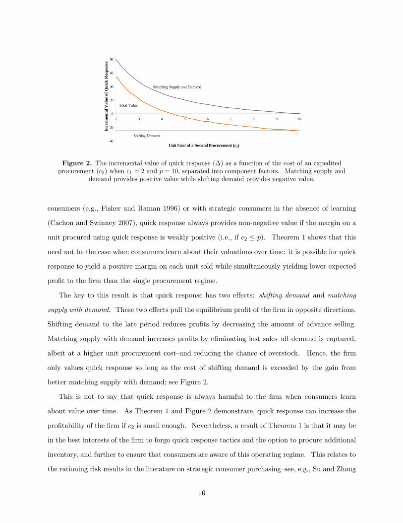
Theorem 1 Let � = �qr��sp be the incremental equilibrium value of quick response. � is strictly

decreasing in the cost of quick response (c2), and if c2 = p, � � 0.

Proof. De�ne �qr (q) = E�pD � c1q � c2 (D � q)+

�, where D is the total demand at the �rm (a

function of �qr). Let �qr be the equilibrium pro�t of the �rm with quick response, and let �sp

be the equilibrium pro�t without QR. Di¤erentiating �qr with respect to c2, we have, from the

Envelope Theorem,

d�qr

dc2=@�qr (q)

@c2

����q=qqr

+@�qr (q)

@q

dqqr

dc2=@�qr (q)

@c2

����q=qqr

:

Note that since �qr contains no dependence on c2, there is no derivative term with respect to �qr.

This impliesd�qr

dc2= �Pr (D > qqr) = �1 + c2 � c1

c2< 0:

Thus, the equilibrium pro�t of the �rm is decreasing in c2. Note that, in the limit as c2 ! p, the

margin on each unit sold that is procured via QR goes to zero. Hence, the �rm�s pro�t e¤ectively

becomes the same as if it did not have QR capabilities, with one caveat: in equilibrium, more

consumers will wait for the late period than if the �rm did not have QR. Thus, limc2!p �qr =

�spj�=�qr � �spj�=�sp , i.e., for large c2 QR yields lower expected pro�ts than the SP regime.

The �rst part of Theorem 1 is natural�the value of a quick response system is decreasing in

the marginal cost of a midseason replenishment. A more surprising result is provided by the

second part of the theorem, which demonstrates that the value of a quick response option (�) can

be negative if c2 = p. Combining both parts of the theorem implies that quick response may

reduce the pro�t of the �rm even if the marginal procurement cost is strictly less than the selling

price. This result stands in contrast to the existing literature on quick response: with non-strategic

15

­40

­20

0

20

40

60

80

2 3 4 5 6 7 8 9 10

Unit Cost of a Second Procurement (c2)

Incr

emen

tal V

alue

 of Q

uick

 Res

pons

e

Matching Supply and Demand

Shifting Demand

Total Value

Figure 2. The incremental value of quick response (�) as a function of the cost of an expeditedprocurement (c2) when c1 = 2 and p = 10, separated into component factors. Matching supply and

demand provides positive value while shifting demand provides negative value.

consumers (e.g., Fisher and Raman 1996) or with strategic consumers in the absence of learning

(Cachon and Swinney 2007), quick response always provides non-negative value if the margin on a

unit procured using quick response is weakly positive (i.e., if c2 � p). Theorem 1 shows that this

need not be the case when consumers learn about their valuations over time: it is possible for quick

response to yield a positive margin on each unit sold while simultaneously yielding lower expected

pro�t to the �rm than the single procurement regime.

The key to this result is that quick response has two e¤ects: shifting demand and matching

supply with demand. These two e¤ects pull the equilibrium pro�t of the �rm in opposite directions.

Shifting demand to the late period reduces pro�ts by decreasing the amount of advance selling.

Matching supply with demand increases pro�ts by eliminating lost sales�all demand is captured,

albeit at a higher unit procurement cost�and reducing the chance of overstock. Hence, the �rm

only values quick response so long as the cost of shifting demand is exceeded by the gain from

better matching supply with demand; see Figure 2.

This is not to say that quick response is always harmful to the �rm when consumers learn

about value over time. As Theorem 1 and Figure 2 demonstrate, quick response can increase the

pro�tability of the �rm if c2 is small enough. Nevertheless, a result of Theorem 1 is that it may be

in the best interests of the �rm to forgo quick response tactics and the option to procure additional

inventory, and further to ensure that consumers are aware of this operating regime. This relates to

the rationing risk results in the literature on strategic consumer purchasing�see, e.g., Su and Zhang

16

(2005) and Debo and van Ryzin (2007). In contrast to the mere reduction of inventory described

in this literature, Theorem 1 implies that the �rm may be better o¤ with an entirely di¤erent

operating policy (Single Procurement vs. Quick Response) when consumers behave strategically�

the inability to react to updated demand information in a timely and responsive way can bene�t the

�rm by generating a credible mismatch between supply and demand and inducing more consumers

to purchase prior to learning their value.

The fact that it may be optimal for the �rm to operate without quick response lends justi�cation

to publicized �limited edition� runs of certain products: such tactics induce consumers who are

otherwise �on the fence� to purchase the product prior to learning if they truly value it, lest no

inventory remain once valuations are revealed. For example, Disney is famous for releasing its

classic �lms on video for very limited periods of time, after which the �lms are �placed in the

Disney vault,�not to be released again for a period of several years. However, as we shall see in

the following sections, this result is sensitive to at least two key assumptions regarding the nature

of the product.

6 Consumer Returns

The preceding analysis assumed that any consumer who purchased an item early had no recourse if

their value for that item turned out to be low�that is, the possibility that a consumer could return

a product if she is dissatis�ed was excluded. In some industries, this assumption is appropriate.

For example, with most types of media (e.g., movies, music, video games, or computer software)

returns are forbidden once an item has been opened (often due to fears of piracy), and Amazon.com

does not allow returns on large televisions due to the logistical challenges of return shipping.

In some cases, however, product returns are a common and important component of �rm strat-

egy. Satisfaction guarantees abound in many settings (clothing, electronics, etc.), with �rms

encouraging customers to try new products �risk free�while promoting generous return policies.

At both Amazon.com and the electronics retailer Best Buy, for example, returns are allowed for full

refunds on most items within a 30 day period; during the holidays this return window is extended

up to a maximum of 90 days. Such policies increase the consumer incentive to purchase early by

reducing the consequences of buying a product which is not valued.

17

In this section, we consider the e¤ect of returns policies on our model of consumer and �rm

learning. Such policies have been addressed�see the discussion in §2�though unlike some previous

papers, we do not address the issue of designing the optimal return policy, but rather we assume

that the �rm o¤ers full refunds to any dissatis�ed customer (possibly for marketing or competitive

reasons) due to the ubiquity of this type of return policy in retailing. (Implications of partial

refunds are discussed at the end of this section.)

Returns occur immediately following the early period, prior to the arrival of late period demand.

In addition to assuming that returns are for full refunds, we assume that returned products are

resalable�that is, the �rm may repackage and resell in the late period any returns that occur from

early period demand. For generality, we assume that consumers who make a return incur a hassle

cost h � 0, and that returns are costly to the �rm, incurring a restocking fee of r � 0 on each

returned item. We assume that p � h � 0, i.e., a dissatis�ed consumer bene�ts from a return.

This implies that if h (�) v � p � 0, then

h (�) v � p+ (1� h (�)) (p� h) � h (�) v � p � 0; (6)

i.e., with returns, high signal consumers have greater incentive to purchase in the early period. We

assume also that returns are enough of a hassle (h is large enough) that low signal consumers still

do not purchase in the early period, i.e., that l (1=2) v � p+ (1� l (1=2)) (p� h) < 0.

We are interested in how the addition of the described return policy changes the results of

§5, speci�cally the results provided in Theorem 1. As we might expect from (6), by increasing

expected surplus in the early period, returns encourage more consumers to purchase early. While

this would seem to bene�t the �rm, the increase in advance purchasing comes at a price: consumers

who purchase in the early period and are dissatis�ed are costly to the �rm, due to the fact that each

returned unit costs the �rm the price of the refund, p, and the restocking fee, r. Thus, the value of

quick response practices�which as we have already mentioned shift demand from the early period

to the late period by lessening the availability risk associated with delaying a purchase�will di¤er

from that derived in the model without returns. The following theorem formalizes this argument.

Theorem 2 Let �r = �qrr � �spr be the incremental equilibrium value of quick response with con-

sumer returns. �r is strictly decreasing in the cost of quick response (c2), and if c2 = p, �r � 0.

18

Proof. The proofs of equilibrium existence and uniqueness are similar to Lemmas 1 and 2, and

are hence omitted. First, we note that with consumer returns, any consumers who purchase in the

early period and are dissatis�ed with the product will return the item. Because we assume that

these products are returned at the start of the late period and are resalable, the total demand to

the �rm is simply �N . Thus, the expected pro�t (without quick response) is

�spr (q) = E�p�N � p (�N � q)+ � c1q � r (1� �)N

Z 1

�spr

(1� x) g (x) dx�;

where �spr refers to the equilibrium critical consumer signal strength with returns, determined by

equating expected �rst and second period surplus, yielding

�spr =h (1� �)

h (1� �) + � (v � p)�1� �b�� :

Immediately we see that (conditional on identical second period �ll rates), �spr � �sp if h � p, i.e.,

holding inventory availability constant, returns encourage more consumers to buy early. As in the

case without returns, quick response induces b� = 1, hence�qrr =

h (1� �)h (1� �) + � (v � p) (1� �)

and �spr � �qrr for any equilibrium belief concerning the �ll rate in the SP regime. Thus, the

expected pro�t with quick response is

�qrr (q) = E�p�N � c2 (�N � q)+ � c1q � r (1� �)N

Z 1

�qrr

(1� x) g (x) dx�:

Clearly �qrr is strictly decreasing in c2 (and hence �r is as well). In addition, for any q,

�qrr (q)� �spr (q)

= E�(p� c2) (�N � q)+ + r (1� �)N

�Z 1

�spr

(1� x) g (x) dx�Z 1

�qrr

(1� x) g (x) dx��:

Because �spr � �qrr , this number is weakly positive if p� c2 � 0, hence for any �xed quantity, quick

response provides non-negative value (and thus the same holds at the optimal quantities), proving

19

the result.

When the �rm allows consumer returns, quick response always increases pro�ts (�r � 0) if

the margin on a unit procured using QR is positive (c2 � p). Recall that in the absence of

consumer returns, quick response may decrease pro�ts (� � 0) even if c2 � p; see Theorem 1.

The two consequences of quick response�shifting demand from the early period to the late period,

and matching supply and demand�move the �rm�s pro�t in opposite directions when returns are

not allowed. Shifting demand in particular hurts the �rm because it means that consumers who

would have purchased with an expectation of positive surplus in the early period may instead not

purchase in the late period after learning their value.

With consumer returns, however, shifting demand increases �rm pro�t, because consumers who

purchase early and are not satis�ed with the product are costly to the �rm (due to the restocking

fee), and the �rm would rather these consumers delay purchasing until they learn their valuations.

Indeed, the above result extends to the case when some or all of the returned goods are not

resalable�in that case, returns are even more costly to the �rm due to the lost opportunity of

reselling a returned product. This result is due to the tendency of consumers to hoard inventory:

given that returns are possible, a consumer would rather purchase an item early and run the risk of

having to return the product, as opposed to delaying the purchase and risking a stock-out. Quick

response reduces the amount of consumer hoarding by increasing overall availability, which in turn

decreases the number of costly returns. See Figure 3 for a graphical depiction of this e¤ect on �rm

pro�t.

This result di¤ers from the existing literature. DeGraba (1995) shows, for instance, that limiting

availability increases the pro�t of the �rm when consumers learn their value over time. Theorem

2 implies that if consumer returns are allowed, exactly the opposite is true: the �rm prefers the

highest level of availability possible (that created by quick response, which provides one hundred

percent availability) in order to minimize the consumer tendency to hoard inventory. The reason

for this di¤erence is that we have assumed that returns are costly to the �rm. Advance selling

by limiting availability (DeGraba 1995) or reducing initial prices (Xie and Shugan 2001) provides

value precisely because dissatis�ed consumers cannot return the product for a full refund. Indeed,

Xie and Shugan (2001) discuss how returns can bene�t the �rm with advance selling�provided that

refunds are not for the full selling price, and indeed that refunds are small enough that the �rm

20

0

10

20

30

40

50

60

70

80

90

100

2 3 4 5 6 7 8 9 10

Unit Cost of a Second Procurement (c2)

Incr

emen

tal V

alue

 of Q

uick

 Res

pons

eMatchingSupply andDemand

Total Value

Shifting Demand

Figure 3. The incremental value of quick response as a function of the cost of an expedited procurement(c2) when c1 = 2 and p = 10, separated into component factors. With costly returns, both matching

supply and demand and shifting demand provide positive value.

pro�ts from every returned unit. In general, if returns are not full refunds, whenever returns

are costly (i.e., whenever the �rm restocking costs plus the di¤erence between the return amount

and the purchase price is positive), Theorem 2 holds, whereas whenever returns are pro�table (the

restocking cost plus the di¤erence between the return amount and purchase price is negative), the

result mirrors that of Theorem 1.

While partial refunds may be reasonable in a booking context (such as airline tickets) in which

service fees for changing reservations are customary, in retailing the vast majority of returns are

for full (or nearly full) refunds due to competitive pressure, and are subsequently costly to �rms�

see Stock et al. (2006) for a discussion of how �rms actively attempt to minimize returns, and

Moorthy and Srinivasan (1995) for a discussion of costly returns. In our model, the interaction of

two e¤ects�consumer learning and costly product returns�implies that the �rm would rather sell

to high type consumers alone in the late period than sell to both types of consumers in the early

period and su¤er a large number of returns. Quick response provides a tool to induce precisely

such behavior, while simultaneously providing value by better matching supply and demand; as a

result, when consumer returns are an issue, quick response yields signi�cant value to the �rm.

21

7 Pricing

In this section, we endogenize pricing in our original model and address how the value of quick

response is a¤ected. We consider two types of pricing: �xed pricing (in which the retailer sets a

single price for both periods) and dynamic pricing (in which the retailer may set di¤erent prices

for each period).

7.1 Fixed Pricing

Unlike the inventory level, price is directly observed by consumers, and hence the �rm acts as a

Stackelberg leader in the price game. Thus, the model with �xed pricing entails a �rst stage in

which the �rm sets the (constant) selling price, and a second stage which behaves identically to the

games analyzed in §§3�5. As a result, given a particular price, the previous results continue to hold

(notably the equilibrium existence results) in the second stage of the game, and we need only analyze

the �rm�s choice of the selling price by comparing expected pro�ts in the inventory/purchasing

subgames using various price levels. The following theorem con�rms that the result of Theorem 1�

quick response may decrease �rm pro�t�continues to hold even when the �rm may set a (constant)

price level.

Theorem 3 Let �fp = �qrfp��

spfp be the incremental equilibrium value of quick response with �xed

pricing. �fp is strictly decreasing in the cost of quick response (c2), and if c2 = v, �fp � 0.

Proof. Note that the existence of an equilibrium is immediate, due to the fact that we have

already shown an equilibrium exists to the inventory/purchasing subgames and the �rm�s expected

payo¤s are bounded (by 0 and EN (v � c1)) and its strategy space is a compact interval [c1; v] in

the pricing supergame ([c2; v] when using quick response�if price is less than c2 but greater than c1,

the �rm will never use QR and reverts to the SP regime). Let �qrfp, pqrfp, and q

qrfp be the equilibrium

pro�t, price, and inventory of the �rm with quick response and �xed pricing, and let �spfp be the

equilibrium pro�t without QR. Di¤erentiating �qrfp with respect to c2, we have, from the Envelope

Theorem,d�qrfpdc2

=@�qrfp@c2

+@�qrfp@p

dpqrfpdc2

+@�qrfp@�

d�qrfpdc2

�@�qrfp@c2

:

22

Observe that either@�qrfp@p = 0 (the �rm prices at an interior optimum) or

dpqrfpdc2

= 0 (the �rm prices

on the boundary, i.e., c2 or v). Unlike the case without pricing,d�qrfpdc2

in general does not equal

zero. This is due to the fact thatdpqrfpdc2

� 0 andd�qrfpdp � 0�in other words, higher costs of quick

response lead to higher prices (a natural result) and higher prices lead to more consumers waiting

until the late period, see equation (4). Because@�qrfp@� � 0 (the more consumers that wait, the lower

the �rm�s pro�ts), it follows that the@�qrfp@�

d�qrfpdc2

� 0. Finally, since

d�qrfpdc2

�@�qrfp@c2

= �Pr�D > qqrfp

�= �1 + c2 � c1

c2< 0;

we �nd that pro�t is decreasing in c2, precisely as in the case without pricing, and �fp is similarly

decreasing in c2. In the limit as c2 ! v, the �rm�s optimal price with QR goes to v, and margin on

each unit sold that is procured via QR goes to zero. Hence, the �rm�s pro�t e¤ectively becomes

the same as if it did not have QR capabilities, with two caveats: it is constrained to price at v

(in the SP regime, the �rm can price anywhere in the interval [c1; v]), and in equilibrium, more

consumers will wait for the late period than if the �rm did not have QR due to the fact that QR

naturally shifts demand. In other words, if c2 = v,

�fp = �qrfp � �

spfp = �qrjp=v � max

p2[c1;v]�sp � �qrjp=v � �

spjp=v � 0

where the last inequality follows from Theorem 1.

The key to this result is the following: when prices are �xed across time, regardless of the

optimal price level, adopting quick response increases the consumer incentive to wait and hence

decreases advance selling and �rm pro�t. The freedom to set the price is of little value in the quick

response regime when c2 is large, as the �rm�s optimal price lies in the interval [c2; v]�if the the price

is lower than c2, then quick response is never used, hence the �rm essentially moves to the single

procurement regime. In the single procurement regime, the �rm remains free to price anywhere

in the interval [c1; v]. When the cost of quick response is large, the quick response regime has two

detrimental e¤ects to the �rm: pricing is constrained and more consumers delay purchasing due to

higher availability. As a result, the single procurement regime becomes even more attractive than

in the exogenous price case. Thus, Theorem 3 mirrors the result of Theorem 1: it is possible for

23

quick response to decrease pro�t (�fp � 0) even when the margin is positive (c2 � p � v).

7.2 Dynamic Pricing

In the dynamic pricing case, we assume that the �rm announces the �rst period price at the start

of the �rst period and announces the second period price at the start of period two. Consumers

develop rational expectations of future prices�that is, they correctly anticipate the price in period

two. We �rst note that if the �rm is free to set di¤erent prices in each period but is constrained

only to mark prices down over time, Theorem 3 continues to hold. The reason is that it is never

optimal in the current model to set a lower price in period two than in period one�lower late period

prices would only encourage more consumers to delay purchasing and hence decrease the amount

of advance selling. Thus, a �rm constrained to mark down over time chooses to set a constant

price, and the model reduces to the �xed pricing case analyzed above.

If the �rm can raise prices over time, however, a di¤erent picture emerges. Let p1 and p2 be

the selling price of the product in periods one and two, respectively. Note that the optimal selling

price in the second period is p2 = v; all consumers know their values, and possess values equal to

v or 0 for the product. Hence, the �rm extracts all surplus from consumers purchasing in period

two by charging the valuation of the high type consumers. Consequently, all consumers have zero

surplus in period two (both high and low types, regardless of whether they successfully procure a

unit), and all consumers with positive �rst period surplus purchase in that period. In general, the

optimal �rst period price satis�es p1 � v, i.e., the �rm charges a lower �rst period price to induce

some advance selling among consumers.

Because all consumers have identically zero surplus in period two, if the �rm adopts quick

response and raises the consumer expectation of availability in the late period (b�), the �rm does

not raise the expected surplus to any consumers from a second period purchase. Thus, quick

response no longer shifts demand�the only e¤ect remaining is matching supply and demand, hence

quick response always has positive value. The following theorem summarizes this result.

Theorem 4 Let �dp = �qrdp � �spdp be the incremental equilibrium value of quick response with

dynamic pricing. �dp is strictly decreasing in the cost of quick response (c2), and if c2 = v,

�dp � 0.

24

Proof. From the preceding discussion, p2 = v, and the existence of an equilibrium to the �rst

period pricing supergame follows from a similar argument to Theorem 3. Combined with the

rational expectations assumption of consumer beliefs concerning future pricing, this implies the

critical � is determined by the solution to ����+(1��)(1��)v � p1 = 0, yielding

�� =p1 (1� �)

� (v � p1) + p1 (1� �)

regardless of the �rm�s operating regime. Note that because the second period price is equal

to v the �rm always makes a pro�t on a unit procured using quick response, and furthermore

�rst period price may lie anywhere in the interval [c1; v]. It is straightforward to see that �dp

is decreasing in c2. Next observe that, as a function of q and p1, pro�t in the SP regime is

�spdp (q; p1) = E [p1min (�1N; q)� c1q], where �1 is a function of p1 (implicitly via ��). Similarly,

pro�t in the QR regime is

�qrdp (q; p1) = E�p1min (�1N; q)� c1q + v

��2N + (�1N � q)+

�� c2 ((�1 + �2)N � q)+

�:

Because �2N+(�1N +�q)+ � (�1N + �2N � q)+ = ((�1 + �2)N � q)+, it follows that �qrdp (q; p1) �

�spdp (q; p1) for any q and p1 (and hence for optimal inventories and prices in the respective regimes).

Thus, �dp � 0 for all c2 � v.

The key to Theorem 4 is that increasing prices over time provides consumers with greater

incentive to purchase early, shifting demand from the late period to the early period. This e¤ect

counteracts the tendency of quick response to shift demand from the early period to the late period.

Thus, dynamic pricing and quick response are complimentary in the sense that they enhance one

another�s value: increasing prices reduces costly demand shifting due to quick response, and quick

response eliminates costly supply/demand mismatches in the second period, mismatches which are

particularly costly under dynamic pricing due to the higher price in period two.

We note that due to the assumption that consumer values follow a two point distribution,

dynamic pricing in the present model completely eliminates strategic waiting in the sense that

all consumers receive zero surplus in period two and hence consumers purchase in period one if

and only if they have positive expected surplus. Should consumers have more than one positive

25

valuation in period two, in general dynamic pricing will not eliminate all strategic waiting, i.e., it

will provide positive surplus to some consumers in period two. In that case, the adoption of quick

response once again shifts demand from the early period to the late period and decreases advance

selling; nevertheless, increasing prices over time continues to reduce the amount of strategic waiting

that occurs and hence minimizes the negative aspects of demand shifting due to quick response.

8 A Manufacturer Selling to Many Retailers

The entirety of the discussion has focused on consumers as end users of the product; alternatively,

we might think of the consumer population as a continuum of retailers, each with (potentially) unit

demand for a product. In this case, the �rm from our model is a manufacturer or supplier, and

the retailers choose whether to stock the product based on their own private signals of whether the

product will be in-demand at their location. This setting is described in the Sport Obermeyer case

study, see Hammond and Raman (1994). In this section, we explore this alternative interpretation

of the model, and consider how a di¤erent perception of a �customer� can produce new insights

from the results.

Consider a single manufacturer introducing a new product to a continuous population of re-

tailers. The manufacturer is uncertain as to how many retailers will consider purchasing the

product, thus N represents the (stochastic) number of retailers in the population and F represents

the manufacturer�s beliefs concerning N . Demand at the retailers follows independent draws from

a two point distribution: with probability � a retailer will face unit demand, and with probability

1 � � the retailer will face zero demand.6 All consumer demand occurs in period two; we may

interpret period one purchases by the retailers as binding pre-orders or advance purchases from the

manufacturer (as in the case of Sport Obermeyer). A consequence of this assumption is that � = 1

for the retailers (because all �consumption,� i.e. sales, occur at a single future date, there should

be no discounting of period two consumption relative to period one consumption).

Each retailer sells the product to consumers for an identical price v (e.g., a manufacturer

suggested retail price). For simplicity, we assume that retailers cannot sell (or purchase) fractions

6This formulation is equivalent to a �xed, deterministic population of retailers N with a stochastic fraction �possessing value v for the product. In this case, all parties know how many retailers are in the market, but thepopularity of the product amongst the consumer population (�) is unknown. As long as the supplier and retailersshare a common belief concerning the distribution of �, all results continue to hold.

26

of a unit, i.e., retailers purchase either one unit or zero units. The remainder of the model remains

the same as that described in §3, with appropriate modi�cations made where necessary, e.g., each

retailer receives a private signal s 2 fl; hg that is an indication of the eventual demand at her

location�low (zero) or high (one).

Previous authors�for example, Cachon (2004), Taylor (2006), Dong and Zhu (2007), and Granot

and Yin (2008)�have addressed the optimal timing of sales within the channel (before or after

forecast updates) and the optimal allocation of inventory risk between a manufacturer and a retailer.

Our model takes a di¤erent tack: given that retailers may purchase at any point in time (i.e., prior

to or after learning demand), what are the manufacturer�s incentives to reduce leadtimes and

create a �exible (upstream) supply chain that allows for additional production and replenishment

in mid-season? In particular, the manufacturer�s decision to adopt quick response will alter retailer

purchasing behavior, just as in the consumer oriented model discussed previously. The question is

then: when does this change in retailer purchasing behavior help�or hurt�the manufacturer?

To answer this question, the following corollary summarizes and restates the results of Theorems

1�4 in a manner consistent with the manufacturer/retailer interpretation of the model. In that

context, consumer returns correspond to manufacturer return or buy-back policies, and dynamic

pricing (particularly increasing prices over time) corresponds to advance purchase contracts, while

constant pricing corresponds to traditional static wholesale price contracts.

Corollary 1 When a manufacturer sells to a continuum of strategic retailers that are free to pur-

chase before or after learning demand:

1. Under a wholesale price contract with exogenous, constant, or non-increasing prices, the man-

ufacturer may not choose to adopt quick response even if c2 is less than the wholesale price.

2. Under a wholesale price contract with unconstrained pricing in both periods (e.g., advance

purchase discounts), the manufacturer always chooses to adopt quick response.

3. Under a buy-back contract, the manufacturer may not adopt quick response if the manufac-

turer�s margin on each unsold (returned) unit is positive.

4. Under a buy-back contract, the manufacturer will adopt quick response if the manufacturer�s

margin on each unsold (returned) unit is negative.

27

As the corollary shows, whether the manufacturer wishes to adopt quick response depends on

the type of supply contract it utilizes with the retailers: if, for instance, the contract allows for

buy-backs (i.e., unsold products can be returned to the supplier, see Cachon 2003), then rapid

production enables the manufacturer to mitigate strategic hoarding of inventory by the retailers

(and subsequent costly returns). On the other hand, if the contract is of the wholesale price

type (i.e., returns are not allowed), the manufacturer has less incentive to adopt quick response�

it can bene�t by advance selling to retailers due to the scarcity engendered by a slower supply

chain. Furthermore, if the manufacturer can o¤er advance-purchase discounts to retailers, the

incentive to adopt quick response increases; by raising prices over time (via the guise of �advance

purchase discounts�) the manufacturer mitigates the degree of strategic waiting by retailers and

hence induces advance purchasing.

9 Discussion

Quick response systems�or, more generally, leadtime reduction and rapid inventory replenishment�

are often suggested as potential panaceas to the ill e¤ects of supply and demand mismatches.

Provided the �xed costs of implementing such systems are low enough, it is argued, the option

to receive additional inventory after a forecast update can only increase a �rm�s pro�t. We have

demonstrated that this basic intuition may be incorrect once the consumer response to increased

availability is taken into account. Though it is a commonly held belief that a faster, more responsive

supply chain is a more pro�table supply chain, we show that such responsiveness is not necessarily

bene�cial to a �rm: when returns are forbidden or when prices are constant, the �rm can exploit

valuation uncertainty by advance selling, and quick response decreases the extent to which the

�rm can advance sell. By operating with rapid ful�llment capabilities, the �rm loses its ability to

credibly restrict inventory to create a stock-out risk, and thus may reduce its overall pro�tability.

The key to this result is that, when consumers learn about product value over time, there

are two components of the value of quick response: matching supply and demand and shifting

demand. The �rst component is well known to increase the pro�t of the �rm by eliminating

lost sales and reducing excess inventory. Shifting demand, on the other hand, can decrease �rm

pro�t by reducing the amount of advance selling and hence the overall demand. In some cases

28

E¤ect of Quick Response on Firm Pro�tModel Demand Matching Demand Shifting Total

Base + � �Base with Returns + + +Base with Fixed Pricing + � �Base with Dynamic Pricing + n=a +

Table 1. A summary of the results on the value of quick response.

(summarized in summarized in Table 1) demand shifting can be reduced (if prices increase over

time) or bene�cial to the �rm (if consumer returns are allowed and are costly). In the former

case, increasing prices mitigate the e¤ects of strategic consumer waiting by reducing second period

surplus and hence inducing more consumers to buy early. In the latter case, consumers are likely to

hoard inventory�they would rather purchase a unit prior to learning their value and risk a return,

than delay purchasing and risk a stock-out. Hoarding is costly for �rms because of explicit costs

of restocking returned inventory and implicit opportunity costs associated with reselling the unit.

By adopting quick response, �rms can mitigate consumer hoarding behavior by signaling high

availability: if stock-outs are unlikely (or impossible) then consumers have little reason to hoard,

which in turn reduces the number of costly returns for the �rm. A consequence of quick response

that was detrimental to the �rm without consumer returns�shifting demand�becomes bene�cial

with returns.

We have also shown that the model of a �rm selling to consumers is analogous to a manufacturer

selling to strategic retailers. In that context, the manufacturer�s incentives to adopt a quick

response production and ful�llment system depends upon the type of contract it employs with the

retailers: quick response is bene�cial when the contract consists of advance purchase discounts or

costly buy-backs (unpro�table on a per-unit basis), while it may be detrimental to the manufacturer

under a constant wholesale price or pro�table buy-backs (pro�table on a per-unit basis).

It is worth noting that quick response is an operational proxy for (more generically) information.

Taken in that context, our results on the value of quick response are essentially results on the value

of accurate information concerning product demand. The fact that quick response sometimes yields

negative value supports the maxim that ignorance can be bliss; the lack of accurate information

on demand can serve as a commitment mechanism to keep inventory scarce and increase advance

selling. Taken together, our results provide insight into when a �rm should adopt a fast supply

29

chain that allows action on improved demand information. Whether selling to consumers or

retailers, the value of matching supply and demand depends not only on the reduction of lost sales

and excess inventory, but also on the strategic response of the �rm�s customers to increased product

availability. This response can be harmful (if advance selling decreases as a result), bene�cial (if

costly returns are allowed and hoarding is an issue), and even diminished or eliminated by the

appropriate pricing strategy (increasing prices over time in the optimal manner). Care must thus

be taken when assessing the value of supply chain responsiveness in order to assess all consequences

of such a strategy�both operational and behavioral.

Acknowledgements. Many thanks to Gérard Cachon, Marshall Fisher, Serguei Netessine,

Senthil Veeraraghavan, Arvind Tripathi, and seminar participants at the University of Pennsylvania,

the University of Texas at Dallas, the University of Rochester, the University of Washington,

New York University, London Business School, Washington University in St. Louis, Northwestern

University, the University of Chicago, Columbia University, Duke University, Stanford University,

and the INFORMS Annual Meeting in Seattle for numerous comments and suggestions.

References

Akan, M., B. Ata, J. Dana. 2007. Revenue management by sequential screening. Working paper,Northwestern University.

Alexandrov, A., M. A. Lariviere. 2006. Are reservations recommended? Working paper, North-western University.

Aviv, Y., A. Pazgal. 2007. Optimal pricing of seasonal products in the presence of forward-lookingconsumers. Forthcoming, Manufacturing Service Oper. Management.

Bikhchandani, S., D. Hirshleifer, I. Welch. 1992. A theory of fads, fashion, custom, and culturalchange as informational cascades. The Journal of the Political Economy 100(5) 992�1026.

Cachon, G. 2004. The allocation of inventory risk in a supply chain: Push, pull, and advance-purchase discount contracts. Management Sci. 50(2) 222�238.

Cachon, G. P. 2003. Supply chain coordination with contracts. Handbooks in Operations Researchand Management Science: Supply Chain Management , chap. 6. North Holland.

Cachon, G. P., R. Swinney. 2007. Purchasing, pricing, and quick response in the presence ofstrategic consumers. Working paper, University of Pennsylvania.

Coughlan, A., C. Savaskan, J. Schulman. 2007. E¤ect of return policies on retail competition.Working paper, Northwestern University.

Dana, J. 1998. Advance-purchase discounts and price discrimination in competitive markets. Jour-nal of the Political Economy 106(2) 395�422.

30

Davis, S., E. Gerstner, M. Hagerty. 1995. Money back guarantees in retailing: Matching productsto consumer tastes. Journal of Retailing 71(1) 7�22.

Debo, L. 2007. In the shadow of the past: Optimal pricing strategies for products with unknownquality and observable price and sales history. Working paper, Carnegie Mellon University.

Debo, L., G. van Ryzin. 2007. Inventories and consumer search behavior when product quality isuncertain. Working paper, Carnegie Mellon University.

DeGraba, P. 1995. Buying frenzies and seller-induced excess demand. The RAND Journal ofEconomics 26(2) 331�342.

Dong, L., K. Zhu. 2007. Two-wholesale-price contracts: Push, pull, and advance-purchase discountcontracts. Manufacturing Service Oper. Management 9(3) 291�311.

Eppen, G. D., A. V. Iyer. 1997. Improved fashion buying with bayesian updating. Oper. Res. 45(6)805�819.

Fisher, M., K. Rajaram, A. Raman. 2001. Optimizing inventory replenishment of retail fashionproducts. Manufacturing Service Oper. Management 3(3) 230�241.

Fisher, M., A. Raman. 1996. Reducing the cost of demand uncertainty through accurate responseto early sales. Oper. Res. 44(1) 87�99.

Gallego, G., Ö. Sahin. 2006. Inter-temporal valuations, product design and revenue management.Working paper, Columbia University.

Granot, D., S. Yin. 2008. Price and order postponement in a decentralized newsvendor model withmultiplicative and price-dependent demand. Oper. Res. 56(1) 121�139.

Hammond, J. H., A. Raman. 1994. Sport Obermeyer Ltd. Case Study, Harvard Business School.

Iyer, A. V., M. E. Bergen. 1997. Quick response in manufacturer-retailer channels. ManagementSci. 43(4) 559�570.

Jerath, K., S. Netessine, S. K. Veeraraghavan. 2007. Revenue management with strategic customers:Last minute selling and opaque selling. Working paper, University of Pennsylvania.

Liu, Q., G. van Ryzin. 2005. Strategic capacity rationing to induce early purchases. Working paper,Columbia University.

Moorthy, S., K. Srinivasan. 1995. Signaling quality with a money-back guarantee: The role oftransaction costs. Marketing Sci. 14(4) 442�466.

Muth, J. F. 1961. Rational expectations and the theory of price movements. Econometrica 29(3)315�335.

Richtel, M. 2007. A year later, the same scene: Long lines for the elusive Wii. The New YorkTimes.

Slatalla, M. 2002. Hot holiday toys: A parent�s strategy. The New York Times.

Stock, J., T. Speh, H. Shear. 2006. Managing product returns for competitive advantage. SloanManagement Review 48(1) 57�62.

31

Stoll, J. 2007. How GM handles a hit: Build fewer. The Wall Street Journal.

Su, X. 2007. Consumer returns policies and supply chain performance. Working paper, Universityof California, Berkeley.

Su, X., F. Zhang. 2005. Strategic consumer behavior, commitment, and supply chain performance.Working paper, University of California, Berkeley.

Taylor, T. 2006. Sale timing in a supply chain: When to sell to the retailer. Manufacturing ServiceOper. Management 8(1) 23�42.

Xie, J., S. M. Shugan. 2001. Electronic tickets, smart cards, and online prepayments: When andhow to advance sell. Marketing Sci. 20(3) 219�243.

32

Technical Appendix to �Selling to Strategic Consumers WhenProduct Value is Uncertain: The Value of Matching Supply and

Demand�

Robert SwinneyGraduate School of Business, Stanford University

518 Memorial Way, Stanford, CA 94305-5015, swinney@stanford.edu

May, 2008

1 Second Period Fill Rate

With a random allocation rule, the actual second period �ll rate is given by

� (q; �) = E�min

�(q � �1N)+ ; �2N

�=�2N

�;

where �1 and �2 are functions of �. Note that

d�1d�

= � (��+ (1� �) (1� �)) g (�) < 0

andd�2d�

= ��g (�) > 0;

and hence d(�1+�2)d� = � (1� �) (1� �) g (�) < 0. Intuitively, higher � implies more consumers

wait until the late period to purchase, hence �rst period demand is decreasing in � while second

period demand is increasing in �. Furthermore, advance selling implies d(�1 + �2)=d� < 0, i.e., if

more consumers wait to purchase, less end up buying the product.

Note that if q < �1N , no customers are served in period two, while if q > �1D1and q > (�1+�2)D,

1

all customers are served in period two. Consequently,

� (q; �) = Pr (q=�1 < N)� 0 + Pr (N < q=(�1 + �2))� 1

+Pr (q=�1 < N < q=(�1 + �2))� E�q � �1N�2N

���� q=�1 < N < q=(�1 + �2)

�:

Thus, the derivative is given by

d� (q; �)

d�= f

�q

�1 + �2

�d

d�

�q

�1 + �2

�+d

d�

Z q=�1

q=(�1+�2)

�q � �1x�2x

�f (x) dx:

Calculating the derivative of the integral yields

Z q=�1

q=(�1+�2)

��q � �1x

�22x

d�2d�

� 1

�2

d�1d�

�f (x) dx� f

�q

�1 + �2

�d

d�

�q

�1 + �2

�:

Thus, the derivative reduces to

d� (q; �)

d�= � 1

�2

Z q=�1

q=(�1+�2)

�q � �1x�2x

d�2d�

+d�1d�

�f (x) dx:

Because d (�1 + �2) =d� < 0 andq��1x�2x

d�2d� +

d�1d� <

d�2d� +

d�1d� , due to the fact that the �ll rate is less

than one, it follows that d�(q;�)d� > 0.

2