semantic 3d reconstruction with finite element bases arxiv
TRANSCRIPT

RICHARD, VOGEL, ET AL.: SEMANTIC 3D RECONSTRUCTION WITH FEM BASES 1
Semantic 3D Reconstruction with FiniteElement BasesAudrey Richard1,†
Christoph Vogel2,†
Maroš Bláha1
Thomas Pock2,3
Konrad Schindler1
1 Photogrammetry & Remote SensingETH Zurich, Switzerland
2 Institute of Computer Graphics & VisionTU Graz, Austria
3 Austrian Institute of Technology
† shared first authorship
Abstract
We propose a novel framework for the discretisation of multi-label problems on ar-bitrary, continuous domains. Our work bridges the gap between general FEM discreti-sations, and labeling problems that arise in a variety of computer vision tasks, includingfor instance those derived from the generalised Potts model. Starting from the popularformulation of labeling as a convex relaxation by functional lifting, we show that FEMdiscretisation is valid for the most general case, where the regulariser is anisotropic andnon-metric. While our findings are generic and applicable to different vision problems,we demonstrate their practical implementation in the context of semantic 3D reconstruc-tion, where such regularisers have proved particularly beneficial. The proposed FEMapproach leads to a smaller memory footprint as well as faster computation, and it con-stitutes a very simple way to enable variable, adaptive resolution within the same model.
1 IntroductionA number of computer vision tasks, such as segmentation, multiview reconstruction, stitch-ing and inpainting, can be formulated as multi-label problems on continuous domains, byfunctional lifting [10, 13, 28, 34, 36]. A recent example is semantic 3D reconstruction (e.g.[4, 18]), which solves the following problem: Given a set of images of a scene, reconstructboth its 3D shape and a segmentation into semantic object classes. The task is particularlychallenging, because the evidence is irregularly distributed in the 3D domain; but it alsopossesses a rich, anisotropic prior structure that can be exploited. Jointly reasoning aboutshape and class allows one to take into account class-specific shape priors (e.g., buildingwalls should be smooth and vertical, and vice versa smooth, vertical surfaces are likely tobe building walls), leading to improved reconstruction results. So far, models for the men-tioned multi-label problems, and in particular for semantic 3D reconstruction, have beenlimited to axis-aligned discretisations. Unless the scenes are aligned with the coordinate
c© 2017. The copyright of this document resides with its authors.It may be distributed unchanged freely in print or electronic forms.
arX
iv:1
710.
0174
9v1
[cs
.CV
] 4
Oct
201
7

2 RICHARD, VOGEL, ET AL.: SEMANTIC 3D RECONSTRUCTION WITH FEM BASES
Figure 1: Semantic 3D model, estimated from aerial views with our FEM method.
axes, this leads to an unnecessarily large number of elements. Moreover, since the evidenceis (inevitably) distributed unevenly in 3D, it also causes biased reconstructions. Thus, it isdesirable to adapt the discretisation to the scene content (as often done for purely geometricsurface reconstruction, e.g. [25]).
Our formulation makes it possible to employ a finer tesselation in regions that are likelyto contain a surface, exploiting the fact that both high spatial resolution and high numericalprecision are only required in those regions. Our discretisation scheme leads to a smallermemory footprint and faster computation, and it constitues a very simple technique to al-low for arbitrary adaptive resolution levels within the same problem. I.e., we can refine orcoarsen the discretisation as appropriate, to adapt to the scene to be reconstructed. Whileour scheme is applicable to a whole family of finite element bases, we investigate two par-ticularly interesting cases: Lagrange (P1) and Raviart-Thomas elements of first order. Wefurther show that the grid-based voxel discretisation is a special case of our P1 basis, suchthat minimum energy solutions of “identical” discretisations (same vertex set) are equivalent.
2 Related WorkSince the seminal work [14] volumetric reconstruction from image data has evolved remark-ably [12, 16, 21, 22, 23, 29, 43, 46]. Most methods use depth maps or 2.5D range scansfor evidence [51, 52], represent the scene via an indicator or signed distance function in thevolumetric domain, and extract the surface as its zero level set, e.g., [30, 42].
Joint estimation of geometry and semantic labels, which had earlier been attempted onlyfor single depth maps [26], has recently emerged as a powerful extension of volumetric 3Dreconstruction from multiple views [1, 4, 18, 24, 39, 44, 45]. A common trait of theseworks is the integration of depth estimates and appearance-based labeling information frommultiple images, with class-specific regularisation via shape priors.
Multi-label problems are in general NP-hard, but under certain conditions on the pair-wise interactions, the original non-convex problem can be converted into a convex one viafunctional lifting and subsequent relaxation, e.g. [10]. This construction was further ex-tended to anisotropic (direction-dependent) regularisers [41]. Moreover, [53] also relaxedthe requirement that the regulariser forms a metric on the label set, yet its construction canonly be applied after discretisation [28]. In this paper, we consider the relaxation in its mostgeneral form [53], but are not restricted to it. The latter construction is also the basis to themodel of [18], whose energy model we adapt for our semantic 3D reconstruction method.Their voxel-based formulation can be seen as a special case of our discretisation scheme.
For (non-semantic) surface reconstruction, several authors prefer a data-dependent dis-cretisation, normally a Delaunay tetrahedralisation of a 3D point cloud [20, 25, 47]. The oc-cupancy states of the tetrahedra are found by discrete (binary) labeling, and the final surfaceis composed of the triangles that separate different labels. Loosely speaking, our proposedmethodology can be seen either as an extension of [18] to arbitrary simplex partitions of thedomain; or as an extension of [25] to semantic (multi-label) reconstruction.

RICHARD, VOGEL, ET AL.: SEMANTIC 3D RECONSTRUCTION WITH FEM BASES 3
We note that regular voxel partitioning of the volume leads to a high memory consump-tion and computation time. Yet, we are essentially reconstructing a 2D manifold in 3D space,and this can be exploited to reduce run-time and memory footprint. [24] use an octree in-stead of equally sized voxels to adapt to the local density of the input data. [4] go one stepfurther and propose an adaptive octree, where the discretisation is refined on-the-fly, duringoptimisation. In our framework the energy is independent of the discretisation, it can thus becombined directly with such an adaptive procedure.
Also volumetric fusion via signed distance functions [32] benefits from irregular tes-selations of 3D space, e.g., octrees [40] or hashmaps [33]. In contrast to our work, thesetarget real-time reconstruction and refrain from global optimisation, instead locally fusingdepth maps. Their input normally is a densely sampled, overcomplete RGB-D video-stream,whereas we deal with noisy and incomplete inputs. To achieve high-quality reconstructionsin our setting, we incorporate semantic information, leading to a multi-label problem.
Our work is based on the finite element method (FEM), e.g. [8, 37]. Introduced by Ritz[38] more than a century ago, and refined by Galerkin and Courant [11], FEM serves tonumerically solve variational problems, by partitioning the domain into finite, parametrisedelements. In computer vision FEM has been applied in the context of level-set methods [49]and for Total Variation [2]. To our knowledge, we are the first to apply it to multi-labeling.
3 MethodThe multi-labeling problem [10, 28, 41, 53] in the domain Ω ⊂ Rd is defined by finding mlabeling functions xi : Ω→0,1, i = 1 . . .m as the solution of:
infxi
m
∑i=1
∫Ω
ρi(z)xi(z)dz+ J(xi), s. t.
m
∑i=1
xi(z) = 1 ∀z ∈Ω, (1)
where ρ models the data term for a specific label at location z ∈ Ω and J denotes a convexregularisation functional that enforces the spatial consistency of the labels. One prominentexample is to chose J := ‖·‖2, known as Total Variation, which penalises the perimeter of theindividual regions [10, 34]. Note that in the two-label case (Potts model), this relaxation isexact after thresholding with any threshold from the open unit interval [10]. Although we areultimately interested in non-metric regularisation, we start with the continuous, anisotropicmodel [41], and postpone the extension to the non-metric case to Sec. 3.5.
3.1 Convex RelaxationThe continuous model allows for an anisotropic regulariser in J: label transitions can bepenalised on the area of the shared surface, as well as on the surface normal direction. Thisis achieved with problem-specific 1-homogeneous functions that emerge from convex sets,so called Wulff-shapes. A relaxation of xi(z) ∈ 0,1 to xi(z) ∈ [0,1] then leads to a convexenergy, which can be written as the following saddle point problem, with primal functions xand dual functions λ :
minxi
maxλ i ∑
i
∫Ω
ρi(z)xi(z)+〈xi(z),∇·λ i(z)〉dz, s.t. λ
i(z)−λj(z)∈W i j,
m
∑i=1
xi(z)=1,xi(z)≥0. (2)
The constraints have to be fulfilled for all z ∈ Ω. In addition to the primal variables xi,we have introduced the dual vector-field λ i : Rd → Rd , whose pairwise differences areconstrained to lie in the convex sets (Wulff-shapes) W i j. By letting these shapes take ananisotropic form, one can then encode scene structure, e.g. [18, 41]. For our problem we

4 RICHARD, VOGEL, ET AL.: SEMANTIC 3D RECONSTRUCTION WITH FEM BASES
demand Neumann conditions at the boundary of Ω, i.e. 〈λ i,ν〉 = 0,∀z ∈ ∂Ω, because thescene will continue beyond our domain (ν is the normal of the domain boundary ∂Ω).
3.2 Finite Element SpacesHere, we can only informally introduce the basic idea of FEM and explain its suitability forproblems of the form (2). We refer to textbooks [8, 15, 27] for a deeper and formal treatment.
One way to solve (2) is to approximate it at a finite number of regular grid points, usingfinite differences. FEM instead searches for a solution in a finite-dimensional vector space;this trial space is a subspace of the space in which the exact solution is defined. To thatend, one chooses a suitable basis for the trial space, with basis functions of finite support, aswell as an appropriate test function space. FEM methods then find approximate solutions tovariational problems by identifying the element from the trial space that is orthogonal to allfunctions of the test function space. For our saddle-point problem, we can instead identifythe trial space with our primal function space and the test space with its dual counterpart.Now, we can apply the same principles, and after discretisation our solution corresponds tothe continuous solution defined by the respective basis. As (2) is already a relaxation of theoriginal problem (1), we do not present an analysis of convergence at this point. Instead, thereader is referred to [2] for an introduction to this somewhat involved topic.
In order to choose a space with good approximation properties and suitable basis func-tions, we tesselate our domain into simplices. More formally, we define M=F,V,S to bea simplex mesh with vertices v∈V,v∈Rd , faces f ∈F defined by d, and simplices s∈ S,defined by d+1 vertices that partition Ω: ∪ksk = Ω,sl ∩ sk = fl,k∈F – i.e. two adjacent sim-plices share only a single face. In this work, for a specific set of vertices V , we select M tobe the corresponding Delaunay tetrahedralisation of Ω and only consider explicit bases. Inparticular, we focus on the Lagrangian (P1) basis, which we use in the following to deriveour framework; and on the Raviart-Thomas (RT) basis. Details for the latter are given in thesupplementary material. The main difference between them is that P1 leads to piecewise lin-ear solutions, which must be thresholded, while RT leads to a constant labeling function persimplex, similar to discrete MAP solutions on CRFs. We note that constant labeling can leadto artefacts, such that the adaptiveness of the FEM model becomes even more important.
The idea of both derivations is similar: (i) select a basis for our primal (P1) or dual (RT)variable set, (ii) find a suitable form via the divergence theorem and Fenchel duality, (iii)extend to the non-metric case, following a principle we term ”label mass preservation”.
3.3 Lagrange ElementsThe Lagrange Pk(M) basis functions describe a conforming polynomial basis of order k+1on our simplex mesh M, i.e. its elements belong to the Hilbert space of differentiable func-tion with finite Lebesgue measure on the domain Ω: Pk(M)⊂ H1(Ω) := p ∈ L2(Ω),∇p ∈(L2(Ω)d). We are interested in the Lagrange basis of first order, P1(M):
P1(M):=p : Ω→R|p∈C(Ω), p(x) :=∑s∈S
cTs x+ds,cs∈Rd ,ds∈R, if x∈s and 0 else. (3)
We construct our linear basis with functions that are defined for each vertex v of a simplex sand can be described in local form with barycentric coordinates:
p1s,v(x) := αv with x = ∑
v∈sαvv, ∑
v∈sαv = 1, αv ≥ 0 if x ∈ s and 0 else. (4)
In each simplex, one can define a scalar field φs(x) ∈ R and compute a gradient in this basisthat will be constant per simplex s (cf. Fig. 2):

RICHARD, VOGEL, ET AL.: SEMANTIC 3D RECONSTRUCTION WITH FEM BASES 5
Figure 2: Left: Illustration of P1 basis function shape. Middle: Scalar field defined as aconvex combination of basis coefficients. Right: Gradient definition in a simplex (5).
φs(x) := ∑v∈s
φv p1s,v and ∇φs = ∑
v∈sφvJv, (5)
with coefficients φv ∈R. Jv ∈Rd denotes a vector that is normal to the face fv opposite nodev, has length | fv||s|d , and points towards the simplex centre. | fv| denotes the area of the face fv,and |s| the volume of the simplex s (cf . Fig. 2 and supplementary material).
3.4 DiscretisationTo apply our Lagrange basis to (2) we first make use of the divergence theorem:∫
Ω
〈xi(z),∇·λ i(z)〉dz =∫
Ω
〈∇xi(z),λ i(z)〉dz−∫
∂Ω
〈ν(z),λ i(z)〉dz︸ ︷︷ ︸=0
. (6)
The latter summand vanishes by our choice of λ . Our approach for a discretisation in theLagrange basis is to choose the labeling function xi ∈ P1(M). This implies that our dualspace consists of constant vector-fields per simplex: λ i
s ∈ Rd . To fulfill the constraint set in(2) we have to verify that, per simplex, the λ i
s lie in the respective Wulff-shape. The simplexconstraints on the xi have to be modeled per vertex. According to (4), the labeling functionsare convex combinations of their values at the vertices and thus stay within the simplex.
We also have to convert the continuous data costs ρ i into a cost per vertex ρ iv, which
can be achieved by convolving the continuous cost with the respective basis function: ρ iv :=∫
Ω ∑s∈N (v) φs(x)ρ i(x)dx. In practice, the integral can be computed by sampling ρ . Integrat-ing the right hand side in (6) over the simplex s leads to a weighting with its volume |s| andthe energy (2) in the discrete setting becomes:
minxi
maxλ i ∑
v,iρ
ivxi
v+∑s,i|s|〈∇xi,λ i
s〉 s.t. (λ is−λ
js)∈W i j ∀i< j, s∈ S,
m
∑i=1
xiv=1, xi
v≥0 ∀v∈V. (7)
3.5 Non-metric extensionTo start with, we note that a non-metric model does not exist in the continuous case [31]and our extension works only after the discretisation into the FEM basis. Please refer tothe supplementary material for an in-depth discussion. Note that our label set of semanticclasses does not have a natural order (in contrast to, e.g., stereo depth or denoised brightness);and also the direction-dependent regulariser is unordered and does not induce a metric cost.To allow for non-metric regularisation we transform the constraint set (λ i−λ j ∈W i j), byintroducing auxiliary variables zi j and Lagrange multipliers yi j, and use Fenchel-Duality:
maxλ i
s ,zi js
minyi j
s∑i< j〈(λ i
s−λj
s )− zi j,yi js 〉−δW i j(zi j
s ) = maxλ i
s
minyi j
s∑i< j−〈(λ i
s−λj
s ),yi js 〉+ ||yi j
s ||W i j . (8)
The dual functions of the indicator functions for the convex sets W i j are 1-homogeneous,of the form || · ||W i j := supw∈W i j wT·. Recall that our label costs are not metric: ∀i< j< k :

6 RICHARD, VOGEL, ET AL.: SEMANTIC 3D RECONSTRUCTION WITH FEM BASES
Figure 3: Left: Without our non-metric extension, optimisation w.r.t. (7) can lower transitioncosts by inserting another label (here 1 between 0 and 2). Right: A solution is to split thegradients of the indicator functions and use direction-dependent variables xi j.
|yi j|W i j + |y jk|W jk ≥ |yik|W ik , does not hold. It was shown [53] that a regulariser of the form(8) transforms any non-metric cost to the metric case. Figure 3 shows an example. Here,an expensive transition between labels 0 and 2 will be replaced by two cheaper transitions0–1 and 1–2. To prevent this, we replace the yi j with direction dependent variables xi j: Werearrange (8) and combine the first summand with the regulariser from (7) to arrive at thefollowing equations (for now ignoring |s|):
∑s
∑i〈∇xi,λ i
s〉−∑i〈λ i
s ,∑j 6=i
(yi j
s [i < j]− y jis [i > j]
)〉,
with [·] denoting Iverson brackets. Let xi j := [yi j]+ and x ji := [−y ji]+, where [·]+ :=max(0, ·).Expanding the gradient (5) we get, per simplex s,
∑i
∑v∈s
λisxi
v([Jv]+− [−Jv]+)−〈λ is , ∑
j:i6= j(xi j− x ji)〉, (9)
which we analyse further to achieve non-metric costs. It was observed in [53] that the xi j ∈Rd can be interpreted as encoding the “label mass” that transitions from label i to label jin a specific direction. Positivity constraints (by definition) on the xi j avoid the transport ofnegative label mass. To anchor transport of mass on the actual mass of label i present at avertex, we introduce the variables xii for the mass that remains at label i, and split the aboveconstraints into two separate sets with the help of additional dual variables θ :
λis(∑
v∈sxi
v[Jv]+−∑j
xi js )+θ
is(∑
v∈sxi
v[−Jv]+−∑j
x jis )+∑
i, jδ≥0(xi j
s ). (10)
Note that this construction is only possible because our elements (simplices) are of strictlypositive volume, in contrast to zero sets in Ω w.r.t. the Lebesgue measure. Finally, we canwrite down our discrete energy in the Lagrange basis defined on the simplex mesh M:
minxi,xi j
maxλ i,θ i ∑
v∈V∑
iρ
ivxi
v +δ∆(xiv)+∑
i< j∑s∈S|s|||xi j
s − x jis ||W i j+
∑s
∑i
θis(∑
v∈sxi
v[−Jv]+−∑j
x jis )+∑
s∑
iλ
is(∑
v∈sxi
v[Jv]+−∑j
xi js )+∑
i, jδ≥0(xi j
s ),(11)
where we have moved the weighting with |s| from the constraint set to the regulariser, anddenote by δ∆(·) the indicator function of the unit simplex.
4 Semantic Reconstruction ModelA prime application scenario for our FEM multi-label energy model (11) is 3D semanticreconstruction. In particular, we focus on an urban scenario and let our labeling functions

RICHARD, VOGEL, ET AL.: SEMANTIC 3D RECONSTRUCTION WITH FEM BASES 7
Figure 4: (a): Wulff-shape (red) with isolines. (b): Minkowski sum of two Wulff-shapes.(c): Simplices are split after inserting new vertices (blue) close to the surface (green). Right:Initialisation of vertices after refinement. (d): Finite differences on a regular grid ([18]) onlycover constraints in green areas, the P1 basis covers all of the domain Ω.
encode freespace (i = 1), building wall, roof, vegetation or ground. Objects that are notexplicitly modeled are collected in an extra clutter class. We define the data cost ρ at a 3D-point x ∈Ω as in [18]: project x into the camera views c ∈ C, and retrieve the correspondingdepth dc(x) and class likelihoods σ i
c(x) from the image space. The σ i are obtained from aMultiBoost classifier. For the depth we look at the difference between the actual distancedc(x) to the camera and the observed depth: d(x,c) := dc(x)− dc(x). For the freespace labelwe always set the cost to 0, for i 6= 1 we define:
ρi(x) := ∑
c∈Cσ
ic(x)[(k−1)ε ≤ d(x,c)≤ kε]+β [|d(x,c)| ≤ kε]sign(d(x,c)). (12)
This model assumes independence of the per-pixel observations, and exponentially dis-tributed inlier noise in the depthmaps, bounded by a parameter kε (k=3 in practice). It isessentially a continuous version of [18], see that paper for details. The parameter ε sets alower bound for the minimal height of the simplices in the tesselation, and thus defines thetarget resolution. The discretisation of the data cost involves a convolution with the respec-tive basis functions, which can be approximated via sampling. Please refer to the supplemen-tary material for details. The Wulff-shapes W i j in (11) are given as the Minkowski sum of theL2-Ball, B2
κ i j := x ∈Rd |‖x‖2 ≤ κ i j and an anisotropic shape Ψi j: W i j := Ψi j⊕B2κ i j . In the
isotropic part, κ i j contains the neighbourhood statistics of the classes. The anisotropic partΨi j models the likelihood of a transition between classes i and j in a certain direction. Fig. 4(a,b) shows an example. For our case we prefer flat, horizontal surfaces at the following labeltransitions: ground-freespace, ground-building, building-roof, ground-vegetation and roof-freespace. A second prior prefers vertical boundaries for the transitions building-freespaceand building-vegetation. More details on the exact form can be found in [18].
The energy (11) is already in primal-dual form, such that we can apply the minimisationscheme of [9], with pre-conditioning [35]. That numerical scheme requires us to projectonto shapes that are Minkowski sums of convex sets. In our case, the sets are simple andthe projection onto each shape can be performed in closed form. We employ a Dykstra-like projection scheme [5], which avoids storing additional variables and proves remarkablyefficient, see supplementary material. We also project the labeling functions xi directly ontothe unit simplex [48]. In order to extract the transition surface, we employ a variant ofmarching tetrahedra (triangles) [42], using the isolevel at 0.5 for each label.
We conclude with two interesting remarks. First, note that a tesselation with a regulargrid [18] can be seen as a simplified version of our discretisation in the P1 Lagrange basis. InFig. 4d we consider the 2D case of the regular grid used in [18]. Here, variables are definedat voxel level. In its dual graph, the vertex set consists of the corners of the primal grid cubes,leading to shifted indicator variables. Per vertex the data term is mainly influenced from thecost in its Voronoi area. Similarly, [18] evaluates the data cost at grid centers, approximately

8 RICHARD, VOGEL, ET AL.: SEMANTIC 3D RECONSTRUCTION WITH FEM BASES
Figure 5: Left: Synthetic 2D scene, colors indicateground (gray), building (red) and roof (yellow). Mid-dle: Control mesh. Right: Example reconstruction.
overallacc. [%]
Tetra Octree MB
Scene 1 84.0 83.9 82.5Scene 2 92.5 92.8 89
Table 1: Quantitative comparisonwith octree model [4] and Multi-Boost input data.
corresponding to integration within the respective Voronoi-area of grid cell. Furthermore,taking finite differences in this regular case corresponds to verifying constraints for only oneof the two triangles (Fig. 4d). The supplementary material includes a more formal analysis.
Second, our formulation is adaptive, in the sense of [4]: Hierarchical refinement of thetesselation can only decrease our energy. Hence, our scheme is applicable when refining themodel on-the-fly. We again must defer a formal proof to the supplementary material and givean intuitive, visual explanation in Fig. 4c . Assume that (x∗,λ ∗,θ ∗) is an optimal solutionfor a certain triplet M = F,V,S. Then a refined tesselation M = F ,V , S can be found byintroducing additional vertices, i.e. V ⊂ V (ideally on the label transition surfaces). To definea new set of simplices, we demand that no faces are flipped, ∀s ∈ S,∃s ∈ S with s∩ s = s.Then one can find a new variable set and data cost ρ with the same energy: We initialisethe new variables from the continuous solution at the respective location, and find new ρvby integration. Subsequent minimisation in the refined mesh can only decrease the energy.The argument works in both ways: Vertices that have the same solution as their adjacentneighbors can be removed without changing the energy. For now we stick to this simplescheme, future work might explore more sophisticated ideas, e.g. along the lines of [17].
5 EvaluationBefore we present results on challenging real 3D data we evaluate our method in 2D on asynthetic dataset. All results are obtained with a multi-core implementation, on a 12-core, 3.5GHz machine with 64GB RAM. For clarity, we only present the Lagrange discretisation. Werefer to the supplementary material for an evaluation of the Raviart-Thomas discretisation.
Input Data. We create a synthetic 2D scene composed of 4 labels: free space, build-ing, ground and roof, surrounded by 17 virtual cameras. To replace depth maps and class-likelihood images, we extract 2D points on the boundary “surface” and assign ground truthlabel costs to each point. For the evaluation in 3D, we use three real-world aerial mappingdata sets. Our method requires two types of input data: depthmaps and pixel-wise classprobabilities (cf . Sec. 4). Moreover, we build a control mesh M around the initially pre-dicted surface, to facilitate our FEM discretisation. Ideally, the control mesh enwraps thetrue surface, using a finer meshing close to it. We densely evaluate the data cost at the ver-tices of a regular data cost grid and let each control vertex accumulate the cost of its nearestneighbours in that grid, to approximate an integration over its Voronoi cell.
2D Lagrange results. Fig. 5 illustrates the result we obtain in a perfect setting. The orig-inal 2D image serves as ground truth for our quantitative evaluation. In this baseline setting,our method achieves 99.8% of overall accuracy and 99.7% of average accuracy, confirmingthe soundness of our Lagrange discretisation. In order to evaluate how our model behavesin a more realistic setting, we conduct a series of experiments where we incrementally adddifferent types of perturbations. Our algorithm is tested against: (i) noise in the initial 2Dpoint cloud, respectively depth maps, (ii) wrong class probabilities and (iii) ambiguous class

RICHARD, VOGEL, ET AL.: SEMANTIC 3D RECONSTRUCTION WITH FEM BASES 9
Figure 6: (a) Illustration of the control mesh foundation. Dots represent values of the data-cost grid and crosses the control vertices. Voronoi cells of the control vertices are depictedwith dashed grey lines and the control mesh with a solid black line. Colors indicate ground(purple), building (red), roof (yellow), free space (cyan) and no datacost (black). (b) Quan-titative evaluation of Lagrange FEM method w.r.t. different degradations of the input data.
probabilities of random subsets, (iv) missing data, e.g. deleting part of a facade to simulateunobserved areas, (v) sparsity of the initial point cloud. Fig. 6b illustrates the influence ofdefective inputs. Under reasonable assumptions on the magnitude of the investigated pertur-bations, we do not observe a significant loss in accuracy. The reconstruction quality starts todecrease if more than half of the input data is misclassified or if the input point cloud is ex-cessively sparse, meaning that >50% of the input is wrong or nonexistent. Average accuracyis naturally more sensitive, due to the larger relative error in small classes.
Influence of the control mesh. Recall from (12) that the data cost of a control vertexv∈V is approximately equal to an integral of ρ over its respective Voronoi area (cf . Fig. 6a,left). Therefore, but also because of the sign change in (12), vertices close to the surfacereceive small cost values and are mainly steered by the regulariser, i.e. these vertices realisea smooth surface. On the other hand, vertices that integrate only over areas with positive ornegative sign determine the inside/outside decision, but are more or less agnostic about theexact location of the surface. We conclude that a sufficient amount of control vertices shouldlie within the band [d− 3ε; d + 3ε] defined by the truncation of the cost function aroundthe observed depth d (cf . (12) and [18]). Ideally control vertices are equally distributedalong each line-of-sight in front and behind the putative match (cf . Fig. 6a, middle column).Undersampling within the near-band can lead to smooth, but inaccurate results (cf . Fig. 6a,top right). Unobserved transitions, e.g. building-ground or roof-building, can also lead toproblems if the affected simplices are too large. To mitigate the effect, we add a few vertices(e.g., a sparse regular grid) on top of the control mesh (cf . Fig. 6a, bottom row). Finally,oversampling each line-of-sight in order to increase the resolution of the control mesh is notrecommended, the right spacing is determined by the noise level and ε and k, chosen in (12).
To conclude, it is an important advantage of the FEM framework that additional verticescan be inserted as required, without changing the energy. In future work we will use thisflexibility to develop smarter control meshes, possibly as a function of the local noise level.
3D Lagrange results. To test our algorithm on real world data, we focus on a datasetfrom the city of Enschede. Complementary results for other datasets are shown in the supple-mentary material. As baseline we use [4], the current state-of-the-art in large-scale semantic

10 RICHARD, VOGEL, ET AL.: SEMANTIC 3D RECONSTRUCTION WITH FEM BASES
3D reconstruction. Due to the lack of 3D ground truth, we follow their evaluation protocoland back-project subsets of the 3D reconstruction to image space, where it is compared to amanual segmentation. As can be seen in Fig. 7 and Tab. 1, the two results are similar in termsof quantitative correctness. We note that measuring labeling accuracy in the 2D projectiondoes not consider the geometric quality of the reconstruction within regions of a single label.
Figs. 1 and 7 show city-modelling results obtained from (nadir and oblique) aerial im-ages. Visually, our models are crisper and less “clay-like”. Compared to axis-aligned dis-cretisation schemes, e.g. [4, 18], our method appears to better represent surfaces not alignedwith the coordinate axis, and exhibit reduced grid aliasing. Both effects are consistent withthe main strength of the FEM framework, to adapt the size and the orientation of the volumeelements to the data. Small tetrahedra, and vertices that coincide with accurate 3D points onsurface discontinuities, favour sharp surface details and crease edges (e.g., substructures onroofs). Faces that follow the data points rather than arbitrary grid directions mitigate aliasingon surfaces not aligned with the coordinate axes (e.g., building walls). The freedom of alocal control mesh unleashes the power of the regulariser in regions where the evidence isweak or ambiguous (e.g., roads, weakly textured building parts).
As already mentioned, our FEM framework can be readily combined with on-the-flyadaptive computation, as used in the baseline [4]. Compared to their voxel/octree model,adaptive refinement is straight-forward, due to the flexibility of the FEM framework, whichallows for the introduction of arbitrary new vertices. As a preliminary proof-of-concept, wehave tested the naive refinement scheme described in Sec. 4. We execute three refinementsteps, where we repeatedly reconstruct the scene and subsequently refine simplices that con-tain surface transitions, while lowering ε by half. Compared to computing everything at thefinal resolution, this already yields substantial savings of 89–97% in memory and 82–93% incomputation time, without any loss in accuracy. Targetting ε ≥ 1√
3(measured w.r.t. a bound-
ing box of 256 units), the runtimes for the tested scenes are 1h04m–1h47m and memoryconsumption is 573–764 MB, on a single machine.
Figure 7: Quantitative evaluation of Scene 1 from Enschede. Left: One of the input images.Middle left: Semantic 3D model. Middle right: Back-projected labels overlayed on theimage. Right: Error map, misclassified pixels are marked in red.
6 ConclusionWe have proposed a novel framework for the discretisation of multi-label problems, andhave shown that, in the context of semantic 3D reconstruction, the increased flexibility ofour scheme allows one to better adapt the discretisation to the data at hand. Our basic ideais generic and not limited to semantic 3D reconstruction or the specific class of regularis-ers. We would like to explore other applications where it may be useful to abandon griddiscretisations and move to a decomposition into simplices.
Acknowledgements: Audrey Richard was supported by SNF grant 200021_157101. Christoph Vogeland Thomas Pock acknowledge support from the ERC starting grant 640156, ’HOMOVIS’.

RICHARD, VOGEL, ET AL.: SEMANTIC 3D RECONSTRUCTION WITH FEM BASES 11
Supplementary Material
This document provides supplementary information to support the main paper. It is struc-tured as follows: Sec. A gives more information about the data and pre-processing used inour experiments, not mentioned in the paper due to lack of space. We hope that the addeddetails will help readers to better appreciate the experimental results. In Sec. B we showcomplementary results obtained with the proposed Lagrange FEM method on other datasets,as well as the full large-scale reconstruction of the city of Enschede. Sec. C contains tech-nical details and formal proofs that had to be omitted in the paper. Finally, Sec. D discussesour formalism for the case of the Raviart-Thomas basis (instead of Lagrange P1), leadingto piecewise constant labels. We also show results in 2D and 3D and a comparison to thoseobtained with the Lagrange basis.
A Input Data
For our real-world experiments, we start from aerial images, cf . Fig. 8. To mitigate foreshort-ening and occlusion, images are acquired in a Maltese cross configuration, with four obliqueviews in addition to the classical nadir view. We orient the images with VisualSFM [50],create depth maps from neighbouring views with Semi-global Matching [6, 19], and predictpixel-wise class-conditional probabilities with a MultiBoost classifier [3]. The classifier istrained on a few hand-labeled images, using the same features as [4]: raw RGB-intensities ina 5×5 window, and 19 geometry features (height, normal direction, anisotropy of structuretensor, etc.) derived from the depth map.
Figure 8: Input data. Left: aerial input images for one position (four oblique views to thenorth, east, south, west, and a nadir image). Middle: oriented image block. Right: depthmap and class probabilities (visualised by maximum-likelihood labels).
B Additional Visualizations
We have tested our semantic reconstruction method on several (synthetic) 2D and (real)3D datasets. Here we provide additional examples to give the reader an impression of thevariety of cases tested in our evaluation. We apply the same prior models as for our 3Dreconstructions. We prefer flat, horizontal structures in the model for the following label
12 RICHARD, VOGEL, ET AL.: SEMANTIC 3D RECONSTRUCTION WITH FEM BASES
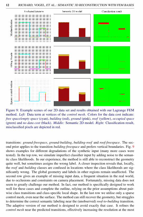
Figure 9: Example scenes of our 2D data set and results obtained with our Lagrange FEMmethod. Left: Data term at vertices of the control mesh. Colors for the data cost indicate:free space/empty space (cyan), building (red), ground (pink), roof (yellow), occupied space(green) and no data cost (black). Middle: Semantic 2D model. Right: Classification result,misclassified pixels are depicted in red.
transitions: ground-freespace, ground-building, building-roof and roof-freespace. The sec-ond prior applies to the transition building-freespace and prefers vertical boundaries. Fig. 9shows examples for different degradations of the synthetic input (many more cases weretested). In the top row, we simulate imperfect classifier input by adding noise to the seman-tic class likelihoods. In our experience, the method is still able to reconstruct the geometryquite well, but sometimes assigns the wrong label. A closer inspection reveals that, locally,the roof and building classes are confused in locations where the class likelihoods are sig-nificantly wrong. The global geometry and labels in other regions remain unaffected. Thesecond row gives an example of missing input data, a frequent situation in the real world,due to occlusions and constraints on camera placement. Fortunately, missing data does notseem to greatly challenge our method. In fact, our method is specifically designed to workwell for these cases and complete the outline, relying on the prior assumptions about pair-wise class transitions and class-specific local shape. In the last row we utilise only a sparsecontrol mesh, even near the surface. The method can still recover the geometry, but strugglesto determine the correct semantic labeling near the (unobserved) roof-to-building transition.The adaptive version of our method is designed to avoid exactly that case. It refines thecontrol mesh near the predicted transitions, effectively increasing the resolution at the most

RICHARD, VOGEL, ET AL.: SEMANTIC 3D RECONSTRUCTION WITH FEM BASES 13
Figure 10: Additional datasets. First row: Original aerial images. Second row: Semantic 3Dmodels obtained with the Lagrange FEM method for Enschede (left), Zürich (middle) andDortmund (right). For the latter, light green denotes an additional class grass and agricul-tural fields.
promising locations.Fig. 10 shows city models obtained from two additional aerial datasets (Zürich, Switzer-
land and Dortmund, Germany), and a further patch from Enschede. These results qualita-tively illustrate that our method works for different image sets and architectural layouts.
Finally, we show the complete semantic 3D reconstruction of Enschede. Fig. 11 showsthe model rendered in an oblique view, together with the corresponding viewpoint in GoogleEarth, to illustrate its accuracy and high level-of-detail.
C Proofs
In this section we give the technical proofs promised in the main paper, as well as furtherdetails about the optimisation. We start with a discussion of the extension to non-metricenergies, and its consequences on the equivalence of continuous and discrete models.
C.1 Non-metric priors: continuous vs. discrete
The main message of this section is that a non-metric model does not exist in the continuousview, unless one imposes additional constraints on the function spaces. We briefly explainwhy: Let’s look at the transition boundary between two labels i and k. Without additionalconstraints, one can always introduce a zero set with label j between the two, i.e., a setwith Lebesgue measure 0 in the domain space. If the transition costs are not metric, thenthe cost for the label pair i,k is potentially higher than the sum of the costs for i, jand j,k. Inserting the zero set will avoid that extra cost and the energy will be under-estimated. In other words, let S be a segmentation of Ω into regions Si and Sk, labeled withi and k respectively. Assume further that their costs do not fulfill the triangle inequalityw.r.t. another label j. Then one can find a sequence of segmentations Sn := Sn
i ,Snj ,S
nk with

14 RICHARD, VOGEL, ET AL.: SEMANTIC 3D RECONSTRUCTION WITH FEM BASES
Figure 11: Large-scale semantic 3D reconstruction of Enschede (Netherlands), computedfrom aerial images with our Lagrange FEM method. Top: View from Google Earth (notused during reconstruction). Bottom: Our model from matching viewpoint.

RICHARD, VOGEL, ET AL.: SEMANTIC 3D RECONSTRUCTION WITH FEM BASES 15
S = limn→∞
(Sn): the label j disappears in the limit, such that limn→∞
infE(Sn) < E(S). Hence,metric transition costs are a necessary condition for the lower semi-continuity of the energyfunctional. Methods that try to resolve the issue with additional constraints on the functionspace, for instance by demanding Lipshitz continuity of the labeling functions, are an activeresearch area, e.g. [7], but are beyond the scope of this work.
The above conceptual problem does have consequences for a practical implementation:Any discretisation of the domain will ultimately consist only of a finite number of elementsof measurable (> 0) volume. Thus, the label j in the example will not disappear completelyfrom the solution, and the computed energy matches the solution. In practice, one can simplyprescribe a minimum edge length in the tesselation, since one cannot refine infinitely. Notethat this also constrains the Lipshitz constant of the labeling functions; they are restricted tovalues between 0 and 1, such that the Lipshitz constant of functions f ∈P1(M) defined on themesh M = V,F,S is bounded by minv∈s,s∈S ||Jv||, cf . (13). Because we utilise a Delaunaytriangulation/tetrahedralisation of the domain and also limit the minimal dihedral angle, afurther constraint on the edge length implies a bound on the Lipshitz constant. Note also, ouranalysis implies that a discrete solution in the non-metric setting does not have a continuouscounterpart, and consequently investigations of the limiting case, i.e., convergence analysisafter infinite refinement of the tesselation, are futile.
C.2 Gradient in the Lagrange basisWe show that gradients of functions in the P1 (Lagrange) basis are constant per simplex sand given by:
∇φs = ∑v∈s
φvJv (13)
Here, the coefficients φv ∈ R and Jv ∈ Rd denote a vector of length | fv||s|d , normal to the facefv opposite to vertex v, and pointing inwards towards the center of the simplex. Recall that| fv| is the area of face fv and |s| is the volume of simplex s.
The gradient can be obtained with basic algebra. First, notice that the gradient of φs in(13) has to fulfill 〈vl− vk,∇φs〉= φvl −φvk , meaning that integration along the edge leads tothe respective change in φs. After collecting a sufficient number of linear equations of thisform, one can directly solve the resulting linear system. Since Jv is, by definition, orthogonalto all edges that do not involve vertex v, we arrive at (13).
Formally, we pick one vertex v of simplex s and compile for l = 1 . . .d (vl 6= v) equationsof the form 〈vl − v,∇φs〉 = φvl −φv. By construction, 〈Jvl ,vk− v〉 = δk=l . The vector Jvl isnormal to face fvl . The scalar product of the edge (vl − v) and the normal is the ”height”within the simplex, so with the chosen scaling of Jvl we have 〈Jvl ,vl− vk〉= 1 for any k 6= l.
Thus multiplying each side of our equation system by a matrix with the vectors Jvl , l =1 . . .d as columns leads to: ∇φs = ∑l Jvl (φvl −φv). If we can show that ∑l Jvl =−Jv, then wearrive at the desired expression (13). For vk,v j 6= v, 〈∑l Jvl ,v j−vk〉= 〈Jvl ,v j〉−〈Jvk ,vk〉= 0and 〈∑l Jvl ,vk−v〉= 〈Jvk ,vk−v〉= 1. All equations are also fulfilled by Jv in place of ∑l Jvl ,which concludes the proof.
C.3 Data Term for Lagrange basisWe again start from the ideas in the main paper. We have to convert the continuous datacosts ρ i into discrete form (in a practical implementation, “continuous” means that the cost

16 RICHARD, VOGEL, ET AL.: SEMANTIC 3D RECONSTRUCTION WITH FEM BASES
can be evaluated at any z ∈ Ω). In our basis representation, we can get discrete cost valuesfor the basis elements by convolving the continuous cost with the respective basis function.For simplicity, we consider the P1 basis function here. Thus, we seek a cost per vertex ρ i
v.In detail we obtain:∫
Ω
xi(z)ρ i(z)dz =∑s
∫sxi
s(z)ρi(z)dz = ∑
s
∫s∑v∈s
φv p1s,v(z)ρ
i(z)dz =
∑v∈V
φv
(∑
s∈N(v)
∫s
p1s,v(z)ρ
i(z)dz
)︸ ︷︷ ︸
:=ρ iv
= 〈ρ iv,x
iv〉. (14)
To numerically compute ρ iv, we sample ρ i at a finite number of locations z ∈ Ω. For
each z we determine into which simplex s it falls, and accumulate the contributions of ρ i(z)over all i = 1 . . .m, weighted by their barycentric coordinates. The final step is to scale ρ i
v
by ∑s∈N(v)|s|d and divide by the sum of weights assigned to vertex v. In other words, we
compute the sample mean and scale it by the area covered by the vertex. In our currentimplementation ρ is sampled at regular grid points, without importance sampling. Thissimple strategy is indeed very similar to the method employed in [4, 18]. There, the datacost is evaluated on a regular grid, by reprojecting grid vertices into each image, computingthe data term, and adding its respective contribution to the grid location. Such a “per-voxelaccumulation” is equivalent to integrating the data cost within the respective Voronoi-areaof a vertex in the dual grid: the latter is proportional to the number of regular samples thatfall into a Voronoi-cell and therefore have the respective vertex as nearest neighbour. Hence,summing the individual contributions directly corresponds to integrating the data term withinthe Voronoi region.
C.4 Grid vs. P1Here, we detail why the grid-based version with finite differences (corresponding to [18])can be seen as an approximation of our proposed FEM discretisation with P1 basis elements,if the vertices (cells) are aligned in a regular grid. Without loss of generality we consider agrid of edge length 1, and note that in this case the gradient for a function f : Ω ⊂ Rd → Rat a grid point x, evaluated with forward differences becomes:
∇ f = ( fx+e1 − fx, . . . , fx+ed − fx)T = ∑
iei fx+ei −∑
iei fx = ∑ fx+eiJx+ei + fxJx, (15)
with ei the unit vector in direction i. We have used the identity ei = Jx+ei , according to thedefinition in Sec. C.2, and obtain the last equality from ∑l Jvl =−Jv, cf . Sec. C.2. This is ex-actly the formula for the gradient of the corresponding P1 function in the simplex defined bythe vertices x,x+ eid
i=1. Accordingly, if implemented as finite differences, the constraintson the dual vector field λ , see Eq. (2) from the paper, are only checked within the respectivesimplex, but not in the whole domain (1/2 of the domain in 2D; 1/6 in 3D). Note also that,with grid-aligned vertices, the simplex in question cannot be part of a partition of Ω ⊂ Rd ,unless d ≤ 2: edges of adjacent faces would intersect.
Fig. 12 illustrates the specific case with d = 2. On the left, the regular grid (green) andthe triangle (simplex, red). Grid centers correspond to vertices in the (triangle-)mesh. Thegrid corresponds to the discretisation used in [18], whereas the simplex mesh is used in this
RICHARD, VOGEL, ET AL.: SEMANTIC 3D RECONSTRUCTION WITH FEM BASES 17
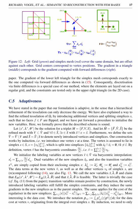
Figure 12: Left: Grid (green) and simplex mesh (red) cover the same domain, but are offsetagainst each other. Grid centers correspond to vertex positions. The gradient in a triangle(middle) corresponds to the gradient computed with forward differences (right).
paper. The gradient of the lower left triangle for the simplex mesh corresponds exactly tothe one computed via forward differences as shown in (15). Consequently, discretisationvia finite differences is a special case of our method, where the elements are layed out on aregular grid, and the constraints are tested only in the upper right triangle (in the 2D case).
C.5 Adaptiveness
We have stated in the paper that our formulation is adaptive, in the sense that a hierarchicalrefinement of the tesselation can only decrease the energy. We have also explained a way tofind the refined tesselation of Ω, by introducing additional vertices and splitting simplices s,such that no faces f ∈ F are flipped; and we have put forward a procedure to initialise thenew variables. Here, we formally prove that the described scheme is sound.
Let (x∗,λ ∗,θ ∗) be the solution for a triplet M = F,V,S. And let M = F ,V , S be therefined mesh with V ⊂ V and ∀s ∈ S,∃s ∈ S with s∩ s = s. Furthermore, we define the setsV = V \V and S = S\S to denote newly introduced vertices and simplices. Our constructionworks by induction, i.e. we introduce one vertex v at a time. The vertex is assumed to lie insimplex s ∈ S, s = vkd+1
k=1 , which is split into simplices skd+1k=1 with sk∩ sl = /0,∀k 6= l. By
definition, vertex v has the barycentric coordinates |sk||s| , i.e. v = ∑
d+1k=1
|sk||s| vk.
We initialize the labeling variables at new vertices v ∈ V via barycentric interpolation:xi
v = ∑vk∈s|sk||s| x
ivk
. Dual variables of the new simplices sk, and also the transition variables
xi j, are simply copied from their enclosing simplex s: λ isk
:= λ is , θ i
sk:= θ i
s and xi jsk
:= xi js .
The data terms at the new vertex v, as well as at the other vertices vk of simplex s, are(re)computed following (14), see also Fig. 13. We call the new variables x, λ , θ and claimthat EM(x∗,λ ∗,θ ∗) = EM(x, λ , θ) and that x, λ , θ is feasible. The latter is trivially the case(cf . Eq. (11) from the paper); transition variables remain positive by construction, the newlyintroduced labeling variables still fulfill the simplex constraints, and they induce the samegradients in the new simplices as in the parent simplex. The same applies for the cost of theregulariser in the new simplices: ∑i< j |s|||x
i js − x ji
s ||W i j = ∑i< j ∑sk∈s |sk|||xi jsk− x ji
sk||W i j . More
interesting is the data cost. We introduce the notation ρv,s :=∫
s p1s,v(z)ρ
i(z)dz for the datacost at vertex v, originating from the integral over simplex s. By induction, we need to only

18 RICHARD, VOGEL, ET AL.: SEMANTIC 3D RECONSTRUCTION WITH FEM BASES
Figure 13: Updated data term after adding a new vertex.
verify the following equality for simplex s, which is split into skd+1k=1 :
∑k
xivk
ρvk,s = ∑k
xivk ∑
j 6=kρvk,s j +∑
jxi
vρv,s j = ∑k
xivk ∑
j 6=kρvk,s j +
|sk||s| ∑
jxi
vkρv,s j (16)
Recall we have ”old” vertices vk, s = vkd+1k=1 and a new vertex v. According to (16), we
must verify:
ρvk,s= ∑j 6=k
ρvk,s j+|sk||s| ∑
jρv,s j⇔
∫sρ(z)p1
s,vk(z)dz=
∫sρ(z) ∑
j 6=kp1
s j ,vk(z)+
|sk||s| ∑
jp1
s j ,v(z)dz.
(17)It is sufficient to show
p1s,vk
(z) = ∑j 6=k
p1s j ,vk
(z)+|sk||s| ∑
jp1
s j ,v(z) ∀z ∈ s. (18)
The right hand side represents a linear function for each skd+1k=1 . We can check if both sides
agree on d + 1 points in each simplex, which is easy to verify. The locations we check –substitute z on both sides of Eq. (18) – are vkd+1
k=1 and v. These are the defining vertices ofthe d+1 simplices skd+1
k=1 . Left and right hand side vanish, except for v and vk. Finally, weget |sk|
|s| for v and 1 for vk on both sides.In our adaptive version, we directly follow the proof and split simplices with the intro-
duction of a single new vertex. We emphasise again that this splitting schedule is merely aproof of concept. The FEM discretisation allows for more sophisticated refinement schemes,e.g., along the lines of [17], or flipping edges according to the energy functional, etc.
C.6 OptimisationThe energy (11) from the paper is given in primal-dual form, optimisation with existing toolsis straight-forward. We apply the minimisation scheme of [9], with pre-conditioning [35].Internally, that algorithm however requires the projection onto the Wulff-shapes W i j, whichis slightly more involved.
C.6.1 Proxmap for the Minkowski sum of convex sets
Recall that, per label pair i, j, our Wulff-shapes are of the form W i j := Ψi j⊕B2κ i j . They
are the Minkowski sum of two simple convex sets. Recall that the Ψi j encode the directiondependent likelihood of a certain label transition. In our case, all Wulff-shapes permit a

RICHARD, VOGEL, ET AL.: SEMANTIC 3D RECONSTRUCTION WITH FEM BASES 19
closed form projection scheme, such that we solve the following sub-problem as proximalstep, independently per simplex s:
argminxi j ,x ji
12||xi j− xi j||2 + 1
2||x ji− x ji||2 + sup
w∈Ψi j⊕B2κi j
wT(xi j− x ji)+ ι≥0(xi j)+ ι≥0(x ji). (19)
For the following derivation we rename the two sets W1 := Ψi j and W2 := B2κ i j . In order to
decouple the argument within the regulariser, we introduce auxiliary variables yk,zk2k=0
and additional Lagrange multipliers µk,λk2k=0, and replace xi j and x ji respectively:
minxi j ,x ji,yk,zk
maxµk,λk
12||xi j− xi j||2 + 1
2||x ji− x ji||2+
∑k∈1,2
supw∈Wk
wT(yk− zk)+ ι≥0(y0)+ ι≥0(z0)−2
∑k=0
λTk (x
i j− yk)−µTk (x
ji− zk).
(20)
Optimality w.r.t. xi j,x ji implies:
xi j = xi j +2
∑k=0
λk and x ji = x ji +2
∑k=0
µk, (21)
which, after reinserting into (20), leads to:
minyk,zk
maxµk,λk
−12||
2
∑k=0
λk− xi j||2 + −12||
2
∑k=0
µk− x ji||2+
supw1∈W1,w2∈W2
wT1(y1− z1)+wT
2(y2− z2)+ ι≥0(y0)+ ι≥0(z0)+2
∑k=0
λTk yk +µ
Tk zk .
(22)
Applying Fenchel-duality yields:
maxµk,λk
minzk
−12||
2
∑k=0
λk− xi j||2 + −12||
2
∑k=0
µk− x ji||2
− ιW1(−λ1)− ιW2(−λ2)− ι≤0(−λ0)− ι≤0(−µ0)+2
∑k=1
(λk +µk)Tzk.
(23)
The latter summand requires λ1 =−µ1 and λ2 =−µ2:
minµ0,λk
12||
2
∑k=0
λk−xi j||2+12||
2
∑k=1
λk+x ji−µ0||2+ιW1(−λ1)+ιW2(−λ2)+ι≥0(λ0)+ι≥0(µ0). (24)
In this last form, we can apply a few iterations of block coordinate descent on the dualvariables and recover the update for xi j,x ji from (21).
D Raviart-Thomas basis
D.1 MethodologyIn this section, we show how to discretise the convex relaxation, Eq. (2) from the paper, forthe case of the Raviart-Thomas basis. For convenience, we restate the energy:
minxi
maxλ i ∑
i
∫Ω
ρi(z)xi(z)+〈xi(z),∇·λ i(z)〉dz, s.t. λ
i(z)−λj(z)∈W i j,
m
∑i=1
xi(z)=1,xi(z)≥0. (25)

20 RICHARD, VOGEL, ET AL.: SEMANTIC 3D RECONSTRUCTION WITH FEM BASES
The Raviart-Thomas basis is chosen as a strong contrast to the (preferred) Lagrangebasis. With Raviart-Thomas functions, we model the dual functions λ in (25), within our trialspace. The Raviart-Thomas RTk(M) basis functions describe a div-conforming polynomialbasis of order k+1, i.e. the divergence of the modeled vector field is continuous acrosssimplices. We again discretise on a simplex mesh M = F,V,S with vertices v ∈V,v ∈ Rd ;faces f ∈ F defined by d vertices; and simplices s ∈ S defined by d + 1 vertices, whichpartition Ω: ∪ksk = Ω,sl ∩ sk = fk,l ∈ F .
RT 0(M) := p : Ω→ Rd |φ(x) := ∑s∈S
φs(x) with φs(x) := csx+ds,cs∈R,ds∈Rd ,
if x∈s and 0 else,and φs(x) is continuous for x ∈ fv(s) in direction νsfv. (26)
Here, we have used νsfv to denote the (outward-pointing) normal of face fv of simplex s. By
convention the face fv is located opposite the vertex v. We construct our linear basis withfunctions that are defined for each face fv in a simplex s, and can be described in a localform as:
φ0s,v(x) := (x− v)
| fv||s|d
if x ∈ s and 0 else,
where we again let | fv| denote the area of the face and |s| the volume of the simplex. Let νsfv
be the normal of face fv in simplex s, then the basis functions fulfill:
〈φ 0s,u(x),ν
sfv〉 := [u = v] ∀x ∈ fv, (27)
with [·] denoting the Iverson bracket.These basis functions make up the global function space by enforcing a consistent orien-
tation. For each face f we can distinguish its two adjacent simplices s+ and s−, by analysingthe scalar product of the vector 1 and the normal ν
s±f of the shared face f (by convention
again pointing outwards of the respective simplex). W.l.o.g., we define sis±f := sign〈νs±
f ;1〉,i.e. s+f νs+
f = s−f νs−f . The global basis functions per face fv are then given by:
φ0s,v :=
sisfv(x− v) | fv||s|d if x ∈ s
0 else.(28)
In each simplex, our vector-field φs(x) ∈ Rd can then be defined in the following manner,with coefficients φ fv ∈ R:
φs(x) := ∑v∈s
φ fvφ0s,v(x).
By construction, cf . (27),(28), the vector-field is continuous along a face x ∈ f in directionof the face normal ν f (of arbitrary, but fixed orientation), i.e. for neighbouring faces s+ ands− we have:
〈φs±(x),ν f 〉= sis±f 〈x− v±,ν f 〉
| f ||s±|d
φ fv± = φ fv± . (29)
Here, v+ is the vertex in simplex s+ opposite to the shared face, and v− is the vertex insimplex s−. Thus, our function in φ is a RT function iff for all neighbouring faces s± wehave φ fv+ = φ fv− . In other words, basis coefficients only exist for faces of the simplices.

RICHARD, VOGEL, ET AL.: SEMANTIC 3D RECONSTRUCTION WITH FEM BASES 21
The variables we are interested in are the labeling functions xi, which are members ofour test function space, composed of piecewise constant functions per simplex:
U0(M) := u : Ω→ R|u(x) := ∑s∈S
us(x), with us(x) = us if x∈s and 0 else. (30)
Before we can utilise our new basis to discretise (25) we need a way to enforce theconstraints on our dual variables λ i(z)−λ j(z) ∈W i j for all z ∈Ω. It is sufficient to enforcethe constraints on the dual functions λ in (25) only at the face midpoints z fv := 1/d ∑w∈ fv wof faces fv ∈ s. This ensures the constraints are also valid for any point in the simplexs. Because the Wulff shapes are convex, it is sufficient to prove that a vector field φ(x) ∈RT 0(M),φ(x) := ∑s∈S φs(x) at any point x ∈ s can be written as a convex combination of thevalues at the face midpoints:
φs(x) = ∑fv∈s
αz fvφ(z fv),with ∑
fv∈sαz fv
= 1.
After some elementary algebra it turns out that, if x = αivi, then αz fv:= (1−d ·αi) encode
this convex combination. Furthermore, the value of φs at a location x ∈ s can be found bylinear combination of basis coefficients at the vertices of s:
φs(x) = ∑v∈s
sisfv(x− v)| fv||s|d
φv. (31)
D.2 DiscretisationWith these relations, we can discretise the energy (25) for labeling functions xi ∈U0(M) anddual vector-field λ i ∈ RT 0(M). First, we convert the continuous data costs ρ i into a costper simplex ρ i
s, which can again be achieved by convolving the cost with the respective (persimplex constant) basis function: ρ i
s :=∫
s us(z)ρ i(z)dz =∫
s ρ i(z)dz. In practice, the integralis computed via sampling. Next, we discretise the second part of our energy with the help ofthe divergence theorem and (29):∫
Ω
xi(z)∇·λ i(z)dx=∑s∈S
∫Sxi
s∇·λ (z)dx=∑s∈S
∫∂S
xis〈λ (z),ν(z)〉dz= ∑
v∈s,s∈Sxi
sλifv | fv|sisfv (32)
As shown, we need to verify the constraints only at face midpoints z fv . The vectors λs(z fv)are linear in the basis coefficients for any z ∈Ω, and the discretised version of (25) becomes
minxi
maxλ i ∑
s∈Sρ
isx
is +∑
v∈s,s∈Sxi
sλifv | fv|sisfv , s.t. λ
is(z fv)−λ
js (z fv) ∈W i j, xi
s ∈ ∆ ∀i< j,v∈s,s∈S.
(33)Here, we let ∆ encode the unit simplex. Finally, for every simplex s, we replace the constraintset ∑i< j λ i
s(z fv)−λj
s (z fv)∈W i j in the same manner as for the Lagrangian basis. We introduceauxiliary variables and Lagrange multipliers yi j
s, fv ,∀i < j, and exploit Fenchel-Duality toobtain
maxλ i
s
minyi j
s∑v∈s
∑i< j||yi j
s, fv ||W i j−∑v∈s
∑i〈λ i
s(z fv), ∑j:i< j
yi js, fv − ∑
j: j<iy ji
s, fv〉=
maxλ i
s
minyi j
s∑v∈s
∑i< j||yi j
s, fv ||W i j−∑v∈s
∑i
λifv
(| fv|sisfv|s|d
[∑f∈s
(z f−v)T(
∑j:i< j
yi js, f− ∑
j: j<iy ji
s, f
)]).
(34)

22 RICHARD, VOGEL, ET AL.: SEMANTIC 3D RECONSTRUCTION WITH FEM BASES
Figure 14: Left: Synthetic 2D scene. Colors indicate ground (gray), building (red) and roof(yellow). Middle: Zoom of the control mesh. Right: Reconstructed semantic 2D model.
Furthermore, recall that we use Neumann conditions at the boundary of Ω, which translatesinto coeffients λ i
f = 0, ∀ f ∈ ∂Ω. Combining (33) and (34), we get the (metric) energy forthe Raviart-Thomas discretisation:
minxi,yi j
maxλ i ∑
s∈S∑
iρ
isx
is + ||y
i js, fv ||W i j + ι∆(xi
s)
+∑v∈s
∑i
λifv | fv|sisfv
(xi
s−1|s|d
[∑f∈s
(z f−v)T(
∑j:i< j
yi js, f− ∑
j: j<iy ji
s, f
)]) (35)
To extend it to non-metric pairwise costs, as in the Lagrangian case, we need to imposeadditional assumptions. One possibility is to utilise basis functions for the dual variables,which are continuous in all directions at the faces. In that case, it is only necessary to checkthe constraints at the faces and not for each face in each simplex, i.e. the variables for yi j
s+, f
and yi js−, f merge into one set. Another possibility is to only force the normal component
along the faces of λ to be contained in the Wulff-shapes. In this direction, RT is alreadycontinuous and the Lagrange multipliers y can be merged. This line of attack leads to ascheme that is remarkably similar to belief propagation on a Markov random field, in thesense that the discretisation lacks a continuous counterpart to begin with, and may lead tostronger grid artifacts. We stop at this point and leave an investigation of such models tofuture work.
D.3 2D results
Fig. 14 illustrates the result we obtain with the Raviart-Thomas FEM method (RT). We usethe same (perfect) baseline setting as for the Lagrange FEM method (P1) in the main paper.In that setting, the RT method achieves 97.5% of overall accuracy and 92.8% of averageaccuracy. While these results confirm that also the RT method is sound, they also show itslimitations compared to the Lagrange basis. Simplices not aligned with object boundaries,straddling multiple labels, will necessarily introduce errors in the reconstruction. Note thatwe do not used edge information to guide the meshing; especially since such informationis not available for our target application, semantic 3D reconstruction. We refer to the 3Dqualitative comparison (cf . Sec. D.4) for a more detailed analysis of the differences betweenthe two methods.
RICHARD, VOGEL, ET AL.: SEMANTIC 3D RECONSTRUCTION WITH FEM BASES 23
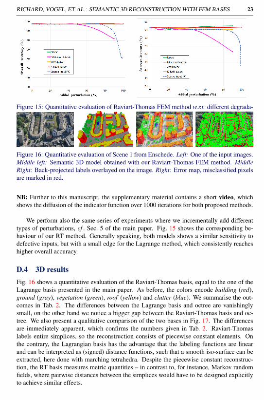
Figure 15: Quantitative evaluation of Raviart-Thomas FEM method w.r.t. different degrada-tions of the input data.
Figure 16: Quantitative evaluation of Scene 1 from Enschede. Left: One of the input images.Middle left: Semantic 3D model obtained with our Raviart-Thomas FEM method. MiddleRight: Back-projected labels overlayed on the image. Right: Error map, misclassified pixelsare marked in red.
NB: Further to this manuscript, the supplementary material contains a short video, whichshows the diffusion of the indicator function over 1000 iterations for both proposed methods.
We perform also the same series of experiments where we incrementally add differenttypes of perturbations, cf . Sec. 5 of the main paper. Fig. 15 shows the corresponding be-haviour of our RT method. Generally speaking, both models shows a similar sensitivity todefective inputs, but with a small edge for the Lagrange method, which consistently reacheshigher overall accuracy.
D.4 3D resultsFig. 16 shows a quantitative evaluation of the Raviart-Thomas basis, equal to the one of theLagrange basis presented in the main paper. As before, the colors encode building (red),ground (gray), vegetation (green), roof (yellow) and clutter (blue). We summarise the out-comes in Tab. 2. The differences between the Lagrange basis and octree are vanishinglysmall, on the other hand we notice a bigger gap between the Raviart-Thomas basis and oc-tree. We also present a qualitative comparison of the two bases in Fig. 17. The differencesare immediately apparent, which confirms the numbers given in Tab. 2. Raviart-Thomaslabels entire simplices, so the reconstruction consists of piecewise constant elements. Onthe contrary, the Lagrangian basis has the advantage that the labeling functions are linearand can be interpreted as (signed) distance functions, such that a smooth iso-surface can beextracted, here done with marching tetrahedra. Despite the piecewise constant reconstruc-tion, the RT basis measures metric quantities – in contrast to, for instance, Markov randomfields, where pairwise distances between the simplices would have to be designed explicitlyto achieve similar effects.

24 RICHARD, VOGEL, ET AL.: SEMANTIC 3D RECONSTRUCTION WITH FEM BASES
Data set Error measure Tetra P1 Tetra RT Octree MB
Scene 1 Overall acc. [%] 84.0 81.9 83.9 82.5Average acc. [%] 81.1 79.1 80.6 81.4
Table 2: Quantitative comparison of our two proposed FEM methods with octree model [4]and MultiBoost input data [3].
Figure 17: Reconstruction with Raviart-Thomas (left) and with the Lagrange basis (right).We deliberately select a low resolution, choose flat shading and plot mesh edges, to accentu-ate the differences. Please refer to the text for details.

RICHARD, VOGEL, ET AL.: SEMANTIC 3D RECONSTRUCTION WITH FEM BASES 25
References[1] Yingze Bao, Manmohan Chandraker, Yuanqing Lin, and Silvio Savarese. Dense object
reconstruction using semantic priors. In CVPR, 2013.
[2] Sören Bartels. Total variation minimization with finite elements: Convergence anditerative solution. SIAM, 50(3), 2012.
[3] D. Benbouzid, R. Busa-Fekete, N. Casagrande, F-D. Collin, and B. Kégl. MULTI-BOOST: a multi-purpose boosting package. JMLR, 2012.
[4] Maros Blaha, Christoph Vogel, Audrey Richard, Jan Dirk Wegner, Thomas Pock,and Konrad Schindler. Large-scale semantic 3d reconstruction: An adaptive multi-resolution model for multi-class volumetric labeling. In CVPR, 2016.
[5] J. P. Boyle and R. L. Dykstra. A method for finding projections onto the intersection ofconvex sets in Hilbert spaces. Lecture Notes in Statistics, 1986.
[6] G. Bradski. The OpenCV Library. Dr. Dobb’s Journal of Software Tools, 2000.
[7] Elie Bretin and Simon Masnou. A new phase field model for inhomogeneous minimalpartitions, and applications to droplets dynamics, 2017.
[8] Franco Brezzi and Michel Fortin. Mixed and Hybrid Finite Element Methods. Springer-Verlag New York, 1991.
[9] Antonin Chambolle and Thomas Pock. A first-order primal-dual algorithm for convexproblems with applications to imaging. JMIV, 40(1), 2011.
[10] Antonin Chambolle, Daniel Cremers, and Thomas Pock. A convex approach to mini-mal partitions. SIAM, 5(4), 2012.
[11] R. Courant. Variational methods for the solution of problems of equilibrium and vibra-tions. Bull. Amer. Math. Soc., 49(1), 01 1943.
[12] D. Cremers and K. Kolev. Multiview stereo and silhouette consistency via convexfunctionals over convex domains. PAMI, 33(6), 2011.
[13] D. Cremers, T. Pock, K. Kolev, and A. Chambolle. Convex Relaxation Techniques forSegmentation, Stereo and Multiview Reconstruction. In Advances in Markov RandomFields for Vision and Image Processing. MIT Press, 2011.
[14] Brian Curless and Marc Levoy. A volumetric method for building complex modelsfrom range images. SIGGRAPH, 1996.
[15] Ricardo G. Durán. Mixed Finite Element Methods. Springer Berlin Heidelberg, 2008.
[16] Yasutaka Furukawa and Jean Ponce. Accurate, dense, and robust multi-view stereopsis.PAMI, 2010.
[17] Eitan Grinspun, Petr Krysl, and Peter Schröder. CHARMS: A Simple Framework forAdaptive Simulation. SIGGRAPH, 2002.

26 RICHARD, VOGEL, ET AL.: SEMANTIC 3D RECONSTRUCTION WITH FEM BASES
[18] Christian Häne, Christopher Zach, Andrea Cohen, Roland Angst, and Marc Pollefeys.Joint 3d scene reconstruction and class segmentation. In CVPR, 2013.
[19] Heiko Hirschmüller. Stereo processing by semiglobal matching and mutual informa-tion. PAMI, 2008.
[20] M. Jancosek and T. Pajdla. Multi-view reconstruction preserving weakly-supportedsurfaces. In CVPR, 2011.
[21] Michael Kazhdan, Matthew Bolitho, and Hugues Hoppe. Poisson surface reconstruc-tion. In EUROGRAPHICS, 2006.
[22] K. Kolev, T. Brox, and D. Cremers. Fast joint estimation of silhouettes and dense 3Dgeometry from multiple images. PAMI, 2012.
[23] Ilya Kostrikov, Esther Horbert, and Bastian Leibe. Probabilistic labeling cost for high-accuracy multi-view reconstruction. In CVPR, 2014.
[24] Abhijit Kundu, Yin Li, Frank Dellaert, Fuxin Li, and James M. Rehg. Joint semanticsegmentation and 3d reconstruction from monocular video. In ECCV, 2014.
[25] Patrick Labatut, Jean-Philippe Pons, and Renaud Keriven. Efficient Multi-View Re-construction of Large-Scale Scenes using Interest Points, Delaunay Triangulation andGraph Cuts. In ICCV, 2007.
[26] L’ubor Ladický, Paul Sturgess, Christopher Russell, Sunando Sengupta, Yalin Bastan-lar, William Clocksin, and Philip Torr. Joint optimisation for object class segmentationand dense stereo reconstruction. In BMVC, 2010.
[27] Mats G. Larson and Fredrik Bengzon. The Finite Element Method: Theory, Implemen-tation, and Applications. Springer Publishing Company, Incorporated, 2013.
[28] Jan Lellmann and Christoph Schnörr. Continuous multiclass labeling approaches andalgorithms. SIIMS, 4(4), 2011.
[29] Shubao Liu and David B. Cooper. Ray Markov random fields for image-based 3dmodeling: Model and efficient inference. In CVPR, 2010.
[30] William E. Lorensen and Harvey E. Cline. Marching cubes: A high resolution 3dsurface construction algorithm. In SIGGRAPH, 1987.
[31] F. Maggi. Sets of Finite Perimeter and Geometric Variational Problems: An Intro-duction to Geometric Measure Theory. Cambridge Studies in Advanced Mathematics.Cambridge University Press, 2012.
[32] Richard A. Newcombe, Shahram Izadi, Otmar Hilliges, David Molyneaux, DavidKim, Andrew J. Davison, Pushmeet Kohli, Jamie Shotton, Steve Hodges, and AndrewFitzgibbon. Kinectfusion: Real-time dense surface mapping and tracking. In ISMAR,Washington, DC, USA, 2011.
[33] Matthias Nießner, Michael Zollhöfer, Shahram Izadi, and Marc Stamminger. Real-time3d reconstruction at scale using voxel hashing. ACM Trans. Graph., 32(6), November2013.

RICHARD, VOGEL, ET AL.: SEMANTIC 3D RECONSTRUCTION WITH FEM BASES 27
[34] Claudia Nieuwenhuis, Eno Töppe, and Daniel Cremers. A survey and comparison ofdiscrete and continuous multi-label optimization approaches for the potts model. IJCV,104(3), 2013.
[35] Thomas Pock and Antonin Chambolle. Diagonal preconditioning for first order primal-dual algorithms in convex optimization. In ICCV, 2011.
[36] Thomas Pock, Daniel Cremers, Horst Bischof, and Antonin Chambolle. Global solu-tions of variational models with convex regularization. SIIMS, 3(4), 2010.
[37] J. Reddy. An Introduction to the Finite Element Method. McGraw-Hill Education,2005.
[38] Walter Ritz. Über eine neue methode zur lösung gewisser variationsprobleme der math-ematischen physik. Journal für die reine und angewandte Mathematik, 1909.
[39] Nikolay Savinov, L’ubor Ladický, Christian Häne, and Marc Pollefeys. Discrete opti-mization of ray potentials for semantic 3d reconstruction. In CVPR, 2015.
[40] F. Steinbruecker, J. Sturm, and D. Cremers. Volumetric 3d mapping in real-time on acpu. In ICRA, 2014.
[41] E. Strekalovskiy and D. Cremers. Generalized ordering constraints for multilabel opti-mization. In ICCV, 2011.
[42] G. Treece. Regularised marching tetrahedra: improved iso-surface extraction. Com-puters & Graphics, 23(4), August 1999. ISSN 00978493.
[43] Ali Osman Ulusoy, Michael J. Black, and Andreas Geiger. Patches, planes and proba-bilities: A non-local prior for volumetric 3D reconstruction. In CVPR, 2016.
[44] Ali Osman Ulusoy, Michael J. Black, and Andreas Geiger. Semantic multi-view stereo:Jointly estimating objects and voxels. In CVPR, 2017.
[45] Vibhav Vineet, Ondrej Miksik, Morten Lidegaard, Matthias Nießner, Stuart Golodetz,Victor A. Prisacariu, Olaf Kähler, David W. Murray, Shahram Izadi, Patrick Perez, andPhilip H. S. Torr. Incremental dense semantic stereo fusion for large-scale semanticscene reconstruction. In ICRA, 2015.
[46] George Vogiatzis, Carlos Hernández Esteban, Philip H. S. Torr, and Roberto Cipolla.Multiview stereo via volumetric graph-cuts and occlusion robust photo-consistency.PAMI, 29(12), 2007.
[47] H. H. Vu, P. Labatut, J. P. Pons, and R. Keriven. High accuracy and visibility-consistentdense multiview stereo. PAMI, 34(5), May 2012.
[48] Weiran Wang and Miguel Á. Carreira-Perpiñán. Projection onto the probabilitysimplex: An efficient algorithm with a simple proof, and an application. CoRR,abs/1309.1541, 2013.
[49] Martin Weber, Andrew Blake, and Roberto Cipolla. Sparse finite elements for geodesiccontours with level-sets. In Tomás Pajdla and Jirí Matas, editors, ECCV, 2004.

28 RICHARD, VOGEL, ET AL.: SEMANTIC 3D RECONSTRUCTION WITH FEM BASES
[50] Changchang Wu. VisualSFM: A visual structure from motion system, 2011.
[51] C. Zach, T. Pock, and H. Bischof. A globally optimal algorithm for robust TV-L1 rangeimage integration. In ICCV, 2007.
[52] Christopher Zach. Fast and high quality fusion of depth maps. 3DV, 2008.
[53] Christopher Zach, Christian Häne, and Marc Pollefeys. What is optimized in convexrelaxations for multilabel problems: Connecting discrete and continuously inspiredMAP inference. PAMI, 2014.