Journal of

Marine Science and Engineering

Article

Semi-Active Structural Control of Offshore WindTurbines Considering Damage Development

Arash Hemmati and Erkan Oterkus *

Department of Naval Architecture, Ocean & Marine Engineering, University of Strathclyde,Glasgow G4 0LZ, UK; arash.hemmati-topkanloo@strath.ac.uk* Correspondence: erkan.oterkus@strath.ac.uk; Tel.: +44-141-548-3876

Received: 29 June 2018; Accepted: 31 August 2018; Published: 5 September 2018�����������������

Abstract: High flexibility of new offshore wind turbines (OWT) makes them vulnerable sincethey are subjected to large environmental loadings, wind turbine excitations and seismic loadings.A control system capable of mitigating undesired vibrations with the potential of modifying itsstructural properties depending on time-variant loadings and damage development can effectivelyenhance serviceability and fatigue lifetime of turbine systems. In the present paper, a modelfor offshore wind turbine systems equipped with a semi-active time-variant tuned mass damperis developed considering nonlinear soil–pile interaction phenomenon and time-variant damageconditions. The adaptive concept of this tuned mass damper assumes slow change in its structuralproperties. Stochastic wind and wave loadings in conjunction with ground motions are applied to thesystem. Damages to soil and tower caused by earthquake strokes are considered and the semi-activecontrol device is retuned to the instantaneous frequency of the system using short-time Fouriertransformation (STFT). The performance of semi-active time-variant vibration control is comparedwith its passive counterpart in operational and parked conditions. The dynamic responses for asingle seismic record and a set of seismic records are presented. The results show that a semi-activemass damper with a mass ratio of 1% performs significantly better than a passive tuned mass damperwith a mass ratio of 4%.

Keywords: offshore wind; structural control; semi-active; tuned mass damper; earthquake

1. Introduction

The wind industry has attracted attention and is growing rapidly due to the environmentalconcerns over conventional energy resources. The offshore wind industry, in particular, is becomingmore attractive because of its advantages over onshore wind. Offshore wind turbines (OWT) aresubject to undesirable vibrations caused by environmental loadings, seismic excitations, and rotorfrequency excitations, and these excessive vibrations need to be minimized to increase serviceabilityand lifetime of the system. A number of structural control devices using vibration control mechanismshave been developed to mitigate the aforementioned excessive vibrations. Tuned mass dampers(TMDs) and tuned liquid dampers (TLDs) are two main vibration control devices widely used.

Various vibration control mechanisms originally from civil engineering field have been proposedto control the level of vibrations in the wind industry. Three main vibration control methods suchas passive, semi-active, and active exist. The applications and descriptions of these methods utilizedin buildings and wind turbine structures were reviewed by Symans and Constantinou [1] and Chenand Georgakis [2]. The passive control system improves damping and stiffness of the main structurewithout the need of employing external forces [3,4]. The vibrations are not tracked via sensorsin this method as curations of this system are constant. This method is widely used due to easyimplementation and maintenance. Active vibration control system is a more sophisticated method

J. Mar. Sci. Eng. 2018, 6, 102; doi:10.3390/jmse6030102 www.mdpi.com/journal/jmse

J. Mar. Sci. Eng. 2018, 6, 102 2 of 22

in which not only mechanical properties are adjusted in the time domain but also external forces areemployed. Thus, active control method requires the presence of active forces from external sources,resulting in high cost and complexity of the system. Semi-active vibration control system is themodified version of the passive control system with the capability of adjusting the properties of thesystem in the time domain with respect to certain properties of vibration forces such as frequencycontent and amplitudes. Vibration amplitudes and frequencies are tracked down using sensorsand signal processing techniques in order to adjust the structural properties. Therefore, semi-activesystem optimizes vibration control capacity without employing external forces. In other words,semi-active system enjoys the best of both active and passive systems; therefore, it can be a morereliable and economically viable option for offshore wind turbines which are subjected to changes intheir natural frequencies.

There is a considerable amount of literature on passive vibration control devices for wind turbines.One of the early studies in this field was done by Enevoldsen and Mørk [5] in which effects ofpassive tuned mass dampers on a 500 kW wind turbine were studied and a cost-effective designwas achieved owing to the implementation of structural control devices. Later on, Murtagh et al. [6]investigated the use of tuned mass dampers (TMD) for mitigating along-wind vibrations of windturbines. They concluded that the dynamic responses could be reduced providing that the device istuned to the fundamental frequency. Colwell and Basu [7] examined effects of tuned liquid columndampers (TLCDs) on offshore wind turbine systems to suppress the excessive vibrations and found thatTLCD can minimize vibrations up to 55% of peak responses of OWTs compared to the uncontrolledsystem. Stewart and Lackner [8] examined the impact of passive tuned mass dampers (PTMD)considering wind–wave misalignment on offshore wind turbine loads for monopile foundations.The results demonstrated that TMDs are effective in damage reduction of towers, especially in side–sidedirections. Stewart and Lackner [9] in another study investigated the effectiveness of TMD systemsfor four different types of platforms including monopile, barge, spar buoy, and tension-leg and theyobserved tower fatigue damage reductions of up to 20% for various TMD configurations. In addition,passive multiple tuned mass dampers (MTMD) were proposed to improve the effectiveness of thevibration control system [10]. Dinh and Basu [10] investigated the use of passive MTMDs for structuralcontrol of nacelle and tower of spar floating wind turbines and concluded that MTMDs are moreeffective in displacement reduction. Whilst passive control methods can reduce the dynamic vibrationsto some extent provided they are tuned properly, they can be easily off-tuned as soon as the dominatingfrequency of the system changes, resulting in ineffectiveness of the system and even increasedvibrations compared to the uncontrolled system. Highly dynamic nature of offshore wind turbinessubjected to a number of dynamic loadings and interacting with nonlinear soil conditions results influctuations in fundamental frequency. Abrupt pulsed nature excitations such as earthquake motionscan lead to degradation of soil stiffness and, consequently, reduction in natural frequency. Furthermore,the cyclic vibration of surrounding soil can cause natural frequency reduction. In addition, naturalfrequency increase might occur when there is stiffening phenomena in certain soil types. Therefore,this raises many questions regarding the use of passive control devices in offshore wind turbines forthe whole lifetime in which there are variations in dominating frequency and the application of moresophisticated vibration control devices needs to be examined.

Active vibration control has also been studied for the application of wind turbines by a numberof researchers [11–17]. Most studies of active control systems for wind turbines were focused on thevibration control of the blades. For example, Stanio and Basu [14] proposed an active vibration controlsystem based on active tendons for wind turbines. The results of their numerical simulations showedthat the proposed control approach is robust in improving the blade responses under vibrations due tothe change of rotational speed of the blades. In addition, Fitzgerald and Basu [17] proposed a cableconnected to an active tuned mass damper for the reduction of in-plane blade vibration and they foundthat the proposed control system mitigates the vibrations of large and flexible blades more effectively.In addition, Kim et al. [18] introduced a robust modal control of lightly damped structures using an

J. Mar. Sci. Eng. 2018, 6, 102 3 of 22

active dynamic vibration absorber. They used a single active electrical dynamic absorber and tested itseffectiveness in control of multiple modes both experimentally and analytically.

The semi-active control mechanism is more suitable for the systems with high time-variantparameters such as offshore wind turbines. Semi-active vibration control devices for the applicationof buildings have been actively studied by a number of researchers [1,19–23] in the last few decades.However, their application in wind energy is a new field. One of the earliest studies on semi-activecontrol mechanism for wind turbines was done by Kirkegaard et al. [24], in which they presented anexperimental and numerical investigation of semi-active vibration control of offshore wind turbinesequipped with a magnetorheological (MR) fluid damper. The authors claimed that using MR dampersfor offshore wind turbines results in considerable reduction of the lateral displacement compared tothe uncontrolled system. Later on, Karimi et al. [25] proposed a controllable valve in tuned liquidcolumn dampers for the application of offshore wind turbines. In addition, the use of semi-active tunedmass dampers in control of flapwise vibrations of wind turbines was examined by Arrigan et al. [26].The authors proposed a frequency-tracking algorithm for retuning the vibration control device andthey observed significant vibration reductions owing to the semi-active mechanism. Furthermore,Weber [27] studied application of an adaptive tuned mass damper concept based on semi-activecontroller using MR dampers. Their results showed that the real-time controlled MR semi-active tunedmass damper is a robust device for reducing structural vibrations. Semi-active control mechanism fortuned liquid column dampers (TLCDs) was also studied by Sonmez et al. [28]. The authors used acontrol algorithm based on short-time Fourier transformation (STFT) and investigated the effectivenessof the proposed device under random excitations. More recently, Sun [29] explored semi-active tunedmass dampers for the NREL (National Renewable Energy Laboratory) 5 MW baseline wind turbineexcited by environmental loadings in conjunction with seismic motions considering post-earthquakedamage to soil and tower stiffnesses. The author demonstrated the superiority of semi-active vibrationcontrol over the passive one in multihazard conditions. Although Sun’s [29] work is well founded,it is limited to only one earthquake record (1994 Northridge Newhall 90) and further study for asuite of earthquake records with different frequency contents and intensities is required. Anotherlimitation of the aforementioned work is that soil–pile interaction was modeled using a simplifiedmethod (closed-form solution) in which the stiffness of embedded pile is considered with a constantrotation and lateral stiffness value in seabed level. More advanced soil–pile interaction model basedon time-variant nonlinear stiffness considering soil damage phenomena can enhance the previousworks. In addition, the effect of semi-active tuned mass dampers on other structural responses such asbase shear and base moment should be investigated.

To fill this gap, this study investigates semi-active tuned mass dampers for offshore wind turbinesunder multihazard conditions considering time-variant nonlinear soil–pile interaction propertiesand time-variant damage. A detailed model of the modern NREL 5 MW wind turbine equippedwith semi-active tuned mass dampers (STMD) is developed. Stochastically wave and wind loadingsin conjunction with seismic loadings are applied to the system and dynamic responses such asdisplacement, base shear, and base moments are investigated. Compared to the previous models,the developed model has the capacity to consider soil–pile interactions more realistically. Furthermore,a suite of seismic records is used with the aim to consider a wider range of seismic characteristics in thesimulations. This paper is organized into five sections. In Section 2, the numerical model of the systemincluding tuned mass dampers, the wind turbine, soil–pile interaction, and the control algorithm ispresented. Section 3 defines the loading sources including wind, wave, and earthquake. The numericalresults and discussions are presented in Section 4 and conclusions are made in Section 5.

J. Mar. Sci. Eng. 2018, 6, 102 4 of 22

2. Model Description

2.1. Tuned Mass Damper Systems

A tuned mass damper (TMD) is a structural control device that consists of a mass, a damper,and a mass attached to a primary structure to control excessive vibration of the primary structureby dissipating energy. The key feature of a TMD is that its frequency is tuned to a particularstructural frequency to mitigate the vibrations when that frequency is excited. The theory of multipledegrees of freedom (MDOF) systems using tuned mass dampers are illustrated and presented in thefollowing section.

The governing equations for the MDOF system in Figure 1 are given as:

m1..u1 + c1

.u1 + k1u− k2(u2 − u1)− c2(

.u2 −

.u1) = p1 −m1

..ug

m2..u2 + c2(

.u2 −

.u1) + k2(u2 − u1)− k3(u3 − u2)− c3(

.u3 −

.u2) = p2 −m2

..ug

...

md..ud + cd

.ud + kdud = −md(

..un +

..ug) (1)

where mi, ci, ki, ui, and pi are mass, damping, stiffness, deflection, and point load for different degreesof freedom of main structure (i = 1, 2, . . . , n), and md, cd, kd, and ud are mass, damping, stiffness,and deflection for the TMD attached to the primary structure. ug is the absolute ground motion due toseismic loadings. The optimal tuned frequency of the TMD, ωd is defined as:

ωd = γω (2)

in which ω is the natural frequency, and γ is the optimal tuning ratio which is determined by thefollowing formula:

γ =1

1 + µ(3)

where µ is the mass ratio as given by the following formula:

µ =md

n∑

i=1mi

(4)

J. Mar. Sci. Eng. 2018, 6, x 5 of 22

Figure 1. Multi degrees of freedom system equipped with a tuned mass damper (TMD).

The schematic configuration of a TMD inside the nacelle is shown in Figure 2.

Figure 2. Schematic figure of TMD in the nacelle.

2.2. Semi-Active Vibration Control Algorithm

There are three main parameters that define a tuned mass damper: mass, stiffness, and damping. Mass of vibration control device cannot be changed in time domain due to practical reasons and only stiffness and damping of the device are altered in time domain depending on instantaneously structural properties of the system and instant dynamic responses. There have been studies on algorithms for time-variant properties of semi-active tuned mass dampers by [21,23,26,28]. In most of the previous studies, the stiffness of semi-active TMD is tuned according to instantaneously identified frequency using short-time Fourier transform and the damping parameters are modulated based on the TMD deflection in each time step.

2.2.1. Varying Stiffness

Stiffness of the semi-active tuned mass damper can be modified based on the identified dominant frequency using short-time Fourier transformation (STFT) function as suggested in the previous studies such as [27,29,30]. Unlike the standard Fourier transform, short-time Fourier transformation adds a time dimension to the base function parameters. A signal x(τ) is multiplied by a moving window function as h(τ − t):

Figure 1. Multi degrees of freedom system equipped with a tuned mass damper (TMD).

J. Mar. Sci. Eng. 2018, 6, 102 5 of 22

The schematic configuration of a TMD inside the nacelle is shown in Figure 2.

J. Mar. Sci. Eng. 2018, 6, x 5 of 22

Figure 1. Multi degrees of freedom system equipped with a tuned mass damper (TMD).

The schematic configuration of a TMD inside the nacelle is shown in Figure 2.

Figure 2. Schematic figure of TMD in the nacelle.

2.2. Semi-Active Vibration Control Algorithm

There are three main parameters that define a tuned mass damper: mass, stiffness, and damping. Mass of vibration control device cannot be changed in time domain due to practical reasons and only stiffness and damping of the device are altered in time domain depending on instantaneously structural properties of the system and instant dynamic responses. There have been studies on algorithms for time-variant properties of semi-active tuned mass dampers by [21,23,26,28]. In most of the previous studies, the stiffness of semi-active TMD is tuned according to instantaneously identified frequency using short-time Fourier transform and the damping parameters are modulated based on the TMD deflection in each time step.

2.2.1. Varying Stiffness

Stiffness of the semi-active tuned mass damper can be modified based on the identified dominant frequency using short-time Fourier transformation (STFT) function as suggested in the previous studies such as [27,29,30]. Unlike the standard Fourier transform, short-time Fourier transformation adds a time dimension to the base function parameters. A signal x(τ) is multiplied by a moving window function as h(τ − t):

Figure 2. Schematic figure of TMD in the nacelle.

2.2. Semi-Active Vibration Control Algorithm

There are three main parameters that define a tuned mass damper: mass, stiffness, and damping.Mass of vibration control device cannot be changed in time domain due to practical reasons and onlystiffness and damping of the device are altered in time domain depending on instantaneously structuralproperties of the system and instant dynamic responses. There have been studies on algorithms fortime-variant properties of semi-active tuned mass dampers by [21,23,26,28]. In most of the previousstudies, the stiffness of semi-active TMD is tuned according to instantaneously identified frequencyusing short-time Fourier transform and the damping parameters are modulated based on the TMDdeflection in each time step.

2.2.1. Varying Stiffness

Stiffness of the semi-active tuned mass damper can be modified based on the identified dominantfrequency using short-time Fourier transformation (STFT) function as suggested in the previous studiessuch as [27,29,30]. Unlike the standard Fourier transform, short-time Fourier transformation adds atime dimension to the base function parameters. A signal x(τ) is multiplied by a moving windowfunction as h(τ − t):

x̂(τ) = x(τ)h(τ − t) (5)

in which x̂(τ) is a weighted signal, τ is the moving time and t is the fixed time.The spectrum S(t, ω) at the fixed time can be defined by applying Fourier transform to x̂(τ):

S(t, ω) =1

2π

∫e−jωt x̂ =

12π

∫e−jωtx(τ)h(τ − t) (6)

and the power spectral density P(t, ω) of time t is calculated as

P(t, ω) = |S(t, ω)|2 = S(t, ω).S(t, ω) (7)

Then, the dominant frequency at time t can be identified using following equations:

ωinst = {ω|P(ti, ω) = max{P(ti, ω)}} (8)

ωid =∑i

k=max{1,i−m+1} ωinst(tk)max{P(tk, ω)}

∑ik=max{1,i−m+1}max{P(tk, ω)}

(9)

J. Mar. Sci. Eng. 2018, 6, 102 6 of 22

where ωid is the dominant frequency at time ti determined through finding the average of instantaneousfrequencies over m time steps (m = 3), and ωinst is the instantaneous frequency. In this study, a movingwindow of 500 time steps (n = 500) with a Hamming window is used. The length of the hammingwindow is taken 1024, L, resulting in the vector of Pi with the size of N × 1, where N = (0.5 * L) + 1.The dominant frequency at each time step is calculated and then stiffness of the tuned mass is retunedusing the dominant frequency as

ktd = kt=0

d (ωidωn

)2

(10)

in which ktd is the time-variant stiffness of tuned mass damper that can be realized through a variable

stiffness device, kt=0d is the initial stiffness of tuned mass damper at the time of zero, and ωn is

the predamage fundamental frequency of the system in which the TMD was tuned to before thedevelopment of any damages.

2.2.2. Varying Damping

The damping of tuned mass dampers can be altered according to the dynamic responses in orderto increase the effectiveness of the device. In the previous studies by Abe and Igusa [31], the authorsinvestigated the time-variant damping for tuned mass dampers and concluded that TMD can improveits performance if the damping of TMD is time-dependent in such a way that its damping valuechanges to zero for the duration in which the relative displacement of TMD is increasing. This resultsin an increase in the efficiency of the system for controlling excessive vibrations. This time-dependentdamping algorithm has been used in other works [23,29,32]. In this method, the relative displacementof TMD is tracked in each time step and if it is larger than that of the previous time step, the dampingof TMD is set to zero, cd

t = 0; otherwise the damping value is set to 2copt, cdt = 2copt. copt is the

optimal value of TMD’s damping which can be determined from an estimation method suggested bySadek et al. [33].

2.3. NREL 5 MW Wind Turbine

The 5 MW NREL wind turbine is considered as it is widely used as the turbine for benchmarkstudies [34]. This turbine is supported by the baseline monopile foundation developed in thesecond phase of Offshore Code Comparison (OC3) project conducted by NREL [35]. The geometricconfiguration of the turbine is shown in Figure 3. The tower and monopile are modeled bythree-dimensional Timoshenko beam theory.

The particulars of the offshore wind turbine are listed in Table 1. Table 2 provides the materialproperties of the steel used in the tower and monopile of the offshore wind turbine. To consideradditional weight of welds, bolts, and paint, the density of the steel in the tower is assumed 8% higherthan that of the regular steel based on the value given in [34].

J. Mar. Sci. Eng. 2018, 6, 102 7 of 22

J. Mar. Sci. Eng. 2018, 6, x 7 of 22

2.3. NREL 5 MW Wind Turbine

The 5 MW NREL wind turbine is considered as it is widely used as the turbine for benchmark studies [34]. This turbine is supported by the baseline monopile foundation developed in the second phase of Offshore Code Comparison (OC3) project conducted by NREL [35]. The geometric configuration of the turbine is shown in Figure 3. The tower and monopile are modeled by three-dimensional Timoshenko beam theory.

Figure 3. Schematic configuration of the offshore wind turbine.

The particulars of the offshore wind turbine are listed in Table 1. Table 2 provides the material properties of the steel used in the tower and monopile of the offshore wind turbine. To consider additional weight of welds, bolts, and paint, the density of the steel in the tower is assumed 8% higher than that of the regular steel based on the value given in [34].

Table 1. Properties of NREL 5 MW baseline turbine.

Turbine Rated Power, Rotor Orientation 5 MW, Upwind, 3 Blades Control System Variable Speed, Collective Pitch

Blade Rotor Diameter, Hub Height 126 m, 90 m Cut-In, Rated, Cut-Out Wind Speed 3 m/s, 11.4 m/s, 25 m/s Cut-In, Rated Rotor Speed 6.9 rpm, 12.1 rpm Hub mass, Blade mass 56,780 kg, 17,740 kg

Nacelle Nacelle Dimensions 18 m × 6 m × 6 m Nacelle Mass 240,000 kg

Tower Base diameter, base thickness 6.0 m, 27 mm Top diameter, top thickness 3.87 m, 19 mm Tower mass 347,460 kg

Figure 3. Schematic configuration of the offshore wind turbine.

Table 1. Properties of NREL 5 MW baseline turbine.

Turbine Rated Power, Rotor Orientation 5 MW, Upwind, 3 Blades

Control System Variable Speed, Collective PitchBlade Rotor Diameter, Hub Height 126 m, 90 m

Cut-In, Rated, Cut-Out Wind Speed 3 m/s, 11.4 m/s, 25 m/sCut-In, Rated Rotor Speed 6.9 rpm, 12.1 rpm

Hub mass, Blade mass 56,780 kg, 17,740 kgNacelle Nacelle Dimensions 18 m × 6 m × 6 m

Nacelle Mass 240,000 kgTower Base diameter, base thickness 6.0 m, 27 mm

Top diameter, top thickness 3.87 m, 19 mmTower mass 347,460 kg

Table 2. Material properties.

Component Density (kg/m3) Young’s Modulus (GPa) Poisson’s Ratio

Tower 8500 210 0.3Monopile 7850 210 0.3

2.4. Soil–Pile Interaction

The nonlinear lateral soil resistance–deflection relationship for sand layers can be defined by ahyperbolic tangent function [36]:

P = Aputanh[

kHApu

y]

(11)

J. Mar. Sci. Eng. 2018, 6, 102 8 of 22

where P is the soil reaction at a given depth, A is a calibration factor which equals to 0.9 for cyclicloading, y is the lateral deflection of soil layers, and k is the initial stiffness coefficient which isdetermined from a function of the angle of internal friction, φ′ [36]. H is depth and pu is the ultimatelateral bearing capacity determined by the following equation:

pu = min

{pus = (C1H + C2D)γH

pud = C3DγH(12)

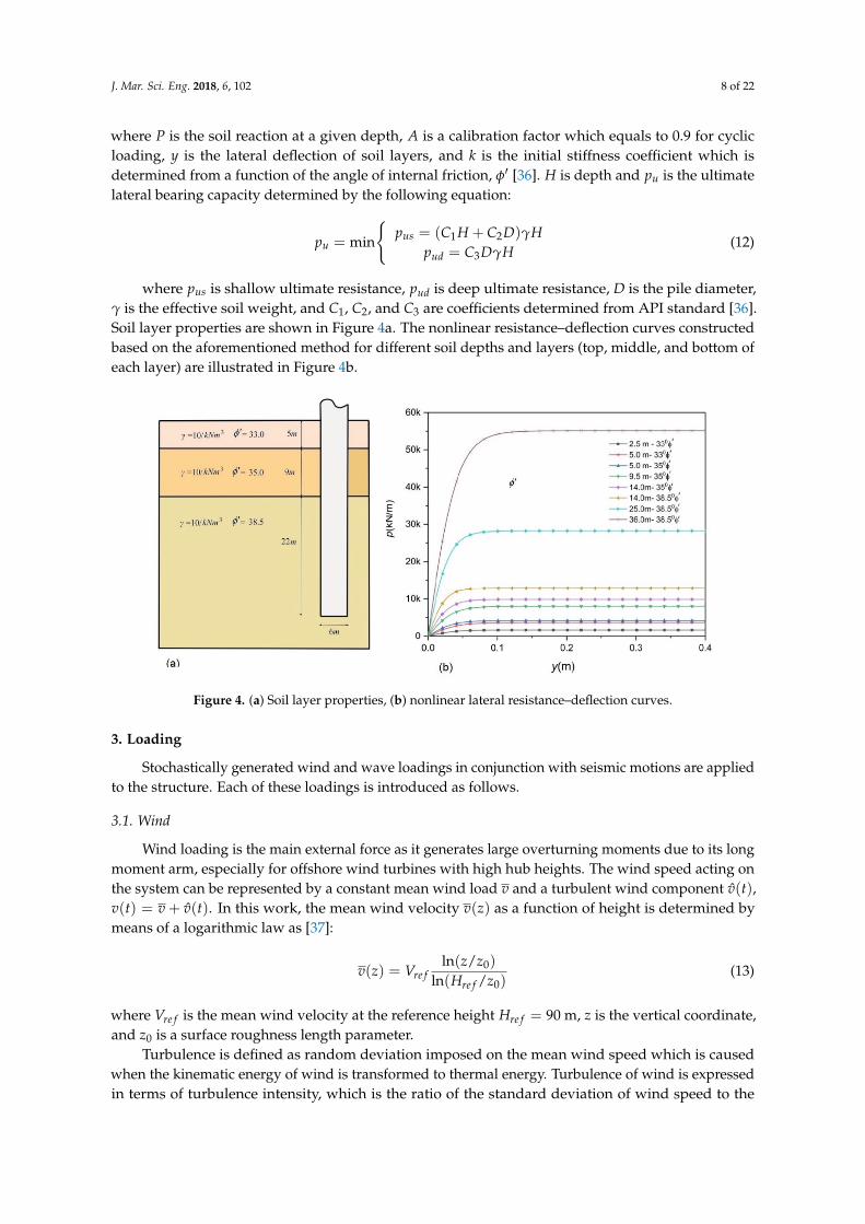
where pus is shallow ultimate resistance, pud is deep ultimate resistance, D is the pile diameter,γ is the effective soil weight, and C1, C2, and C3 are coefficients determined from API standard [36].Soil layer properties are shown in Figure 4a. The nonlinear resistance–deflection curves constructedbased on the aforementioned method for different soil depths and layers (top, middle, and bottom ofeach layer) are illustrated in Figure 4b.

J. Mar. Sci. Eng. 2018, 6, x 8 of 22

Table 2. Material properties.

Component Density (kg/m3) Young’s Modulus (GPa) Poisson’s Ratio Tower 8500 210 0.3

Monopile 7850 210 0.3

2.4. Soil–Pile Interaction

The nonlinear lateral soil resistance–deflection relationship for sand layers can be defined by a hyperbolic tangent function [36]:

tanhuu

kHP Ap y

Ap=

(11)

where P is the soil reaction at a given depth, A is a calibration factor which equals to 0.9 for cyclic loading, y is the lateral deflection of soil layers, and k is the initial stiffness coefficient which is

determined from a function of the angle of internal friction, φ′ [36]. H is depth and up is the ultimate lateral bearing capacity determined by the following equation:

=+=

=HDCp

H)DCHC(pminp

3ud

21usu γ

γ (12)

where usp is shallow ultimate resistance, udp is deep ultimate resistance, D is the pile diameter, γ is the effective soil weight, and 1C , 2C , and 3C are coefficients determined from API standard [36]. Soil layer properties are shown in Figure 4a. The nonlinear resistance–deflection curves constructed based on the aforementioned method for different soil depths and layers (top, middle, and bottom of each layer) are illustrated in Figure 4b.

Figure 4. (a) Soil layer properties, (b) nonlinear lateral resistance–deflection curves.

3. Loading

Stochastically generated wind and wave loadings in conjunction with seismic motions are applied to the structure. Each of these loadings is introduced as follows.

3.1. Wind

Wind loading is the main external force as it generates large overturning moments due to its long moment arm, especially for offshore wind turbines with high hub heights. The wind speed acting on the system can be represented by a constant mean wind load v and a turbulent wind

Figure 4. (a) Soil layer properties, (b) nonlinear lateral resistance–deflection curves.

3. Loading

Stochastically generated wind and wave loadings in conjunction with seismic motions are appliedto the structure. Each of these loadings is introduced as follows.

3.1. Wind

Wind loading is the main external force as it generates large overturning moments due to its longmoment arm, especially for offshore wind turbines with high hub heights. The wind speed acting onthe system can be represented by a constant mean wind load v and a turbulent wind component v̂(t),v(t) = v + v̂(t). In this work, the mean wind velocity v(z) as a function of height is determined bymeans of a logarithmic law as [37]:

v(z) = Vre fln(z/z0)

ln(Hre f /z0)(13)

where Vre f is the mean wind velocity at the reference height Hre f = 90 m, z is the vertical coordinate,and z0 is a surface roughness length parameter.

Turbulence is defined as random deviation imposed on the mean wind speed which is causedwhen the kinematic energy of wind is transformed to thermal energy. Turbulence of wind is expressedin terms of turbulence intensity, which is the ratio of the standard deviation of wind speed to the

J. Mar. Sci. Eng. 2018, 6, 102 9 of 22

mean wind speed. Kaimal spectrum Sv( f ) [38] is adopted in this study to calculate the turbulent windvelocity as follows:

Sv( f ) =4I2Lk

(1 + 6 f Lk/v)5/3 (14)

where I is the wind turbulence intensity, f is the frequency (Hz), and Lk is an integral length scaleparameter. In this study, the stochastic wind profile is generated using Turbsim code [39] over arectangular grid with 961 points (31 × 31) based on Equations (13) and (14). Then, the aerodynamicloadings on the blades are computed in FAST (Version 8.15, NREL, Golden, CO, USA) [40]code using the aforementioned wind profile based on blade element momentum (BEM) theory.Finally, the generated wind loading time history is used in the developed code to consideraerodynamic loadings.

3.2. Sea Wave Load

Wave loading acting on cylindrical structural members of fixed platforms can be obtained usingMorison’s equation [37] as the sum of inertia and drag forces. The transverse sea wave force acting ona strip of a length dz is given by the sum of inertia and drag force terms as the following equation [41]:

dF =ρw

2CdDυ|υ|dz +

πD2

2Cmρw

.υdz (15)

where Cd and Cm are the drag and inertia coefficients, respectively (Cd = 1.2 and Cm = 2 in the currentstudy), D is the diameter of the member,

.υ and υ are horizontal acceleration and velocity of fluid

particles induced by wave excitations, and ρw is water density (1025 kg/m3).The spectrum developed through the Joint North Sea Wave Observation Project (JONSWAP) is

used to generate wave time histories [42] as follows:

Sηη( f ) =αg2

f 5 exp[−5

4(

fm

f)4]

γexp [− ( f− fm)2

2σ2 fm2 ](16)

in which Sηη( f ) is JONSWAP spectrum, η is the function of water surface elevation, γ is the peakenhancement factor (3.3 for the north sea), g is the acceleration of gravity, and f is the wave frequency(Hz). The constants in this equation can be defined as

α = 0.076(

U102/Fg

)0.22(17)

fm = 11(v10F/g2)−1/3

/π (18)

and

σ =

{0.07,0.09,

f ≤ fm

f > fm(19)

where U10 is the mean wind velocity at 10 m from the sea surface, and F is the fetch length in whichthe wind blows without any change of direction.

Then, total wave force acting on the structural members can be calculated as

Ff (t) =∫ d

0dFφ f (z)dz (20)

where dF is the wave loading on the member mentioned in Equation (15), and φ f is the shape functionof the offshore structure subjected to wave loading, d is the depth of the water surface, and z is thevertical direction.

J. Mar. Sci. Eng. 2018, 6, 102 10 of 22

3.3. Seismic Excitation

To simulate seismic excitations on the offshore wind turbines, time series of acceleration of strongground motions during past earthquake events are used. Two horizontal directions are selected torepresent the behavior of earthquake events. In this study, sloshing of water surrounding the structureis ignored as it is believed to have insignificant effects. The seismic records are selected from the PacificEarthquake Engineering Research centre (PEER) Database [43] and listed in Table 3. The magnitudesof the seismic ground motions selected in this study vary between 5.5 and 7.5.

Table 3. Seismic records.

ID Earthquake Magnitude Year Record Station Soil Type

1 Kobe, Japan 6.9 1995 Kobe University B2 Northridge-01 6.69 1994 17645 D3 Northridge-Landers 7.28 1992 17645 Saticoy St. D4 Northridge-Narrows-01 5.99 1987 17645 Saticoy St. D5 Tabas, Iran 7.35 1978 Tabas C6 Manjil, Iran 7.37 1990 Abbar E7 Manjil, Iran 7.37 1990 Abhar D8 Manjil, Iran 7.37 1990 Qazvin C9 Manjil, Iran 7.37 1990 Rudsar D

10 Erzican, Turkey 6.69 1992 Erzincan D11 Loma Prieta 6.93 1989 Apeel 10-Skyline D12 Loma Prieta 6.93 1989 Apeel 2-Redwood City E13 Cape Mendocino 7.01 1992 Cape Mendocino B14 Cape Mendocino 7.01 1992 Eureka-Myrtle & West C15 Cape Mendocino 7.01 1992 Fortuna-Fortuna Blvd. D16 Cape Mendocino 7.01 1992 Petrolia D17 Cape Mendocino 7.01 1992 Shelter Cove Airport D18 Landers 7.28 1992 Amboy C19 Landers 7.28 1992 Baker Fire Station D20 Landers 7.28 1992 Bell Gardens-Jaboneria D21 Imperial Valley-06 6.53 1979 Aeropuerto Mexicali C22 Imperial Valley-06 6.53 1979 Agrarias D24 Imperial Valley-06 6.53 1979 Bonds Corner D24 Imperial Valley-06 6.53 1979 Brawley Airport C25 Imperial Valley-06 6.53 1979 Calexico Fire Station D26 Imperial Valley-06 6.53 1979 Calipatria Fire Station D27 Imperial Valley-06 6.53 1979 Cerro Prieto D28 Imperial Valley-06 6.53 1979 Chihuahua D29 Imperial Valley-06 6.53 1979 Coachella Canal #4 C30 Imperial Valley-06 6.53 1979 Compuertas C

4. Numerical Results and Discussions

4.1. Model Verification

In this section, the results of the natural frequency and dynamic analyses using the developedmodel in MATLAB (R2017a, MathWorks, Natick, MA, USA) are verified. To carry out natural frequencyanalysis, the stiffness of nonlinear soil–pile interaction is linearized by taking initial stiffness ofthe p–y curves [44]. The resulting first and second natural frequencies are listed in Table 4 andcompared with the results of the model created by commercial finite element software ANSYS(16, Canonsburg, PA, USA) and the results from the literature [45]. There is good agreement betweenthe results of natural frequency analyses.

J. Mar. Sci. Eng. 2018, 6, 102 11 of 22

Table 4. Natural frequency analysis results (Hz).

Mode Code ANSYS Dong Hywan Kim et al. [45]

1nd Fore–aft 0.235 0.234 0.2341nd Side-to-side 0.235 0.234 0.233

2nd Fore–aft 1.426 1.426 1.4062nd Side-to-side 1.426 1.426 1.515

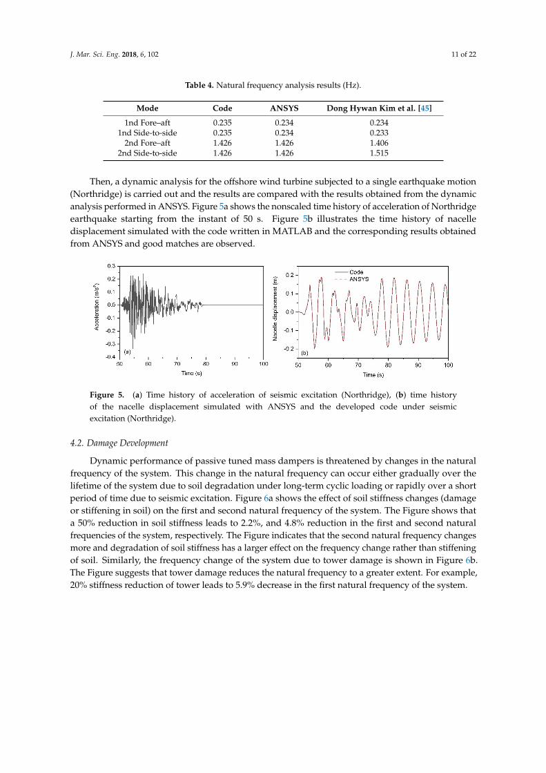
Then, a dynamic analysis for the offshore wind turbine subjected to a single earthquake motion(Northridge) is carried out and the results are compared with the results obtained from the dynamicanalysis performed in ANSYS. Figure 5a shows the nonscaled time history of acceleration of Northridgeearthquake starting from the instant of 50 s. Figure 5b illustrates the time history of nacelledisplacement simulated with the code written in MATLAB and the corresponding results obtainedfrom ANSYS and good matches are observed.

J. Mar. Sci. Eng. 2018, 6, x 11 of 22

4. Numerical Results and Discussions

4.1. Model Verification

In this section, the results of the natural frequency and dynamic analyses using the developed model in MATLAB (R2017a, MathWorks, Natick, MA, USA) are verified. To carry out natural frequency analysis, the stiffness of nonlinear soil–pile interaction is linearized by taking initial stiffness of the p–y curves [44]. The resulting first and second natural frequencies are listed in Table 4 and compared with the results of the model created by commercial finite element software ANSYS (16, Canonsburg, PA, USA) and the results from the literature [45]. There is good agreement between the results of natural frequency analyses.

Table 4. Natural frequency analysis results (Hz).

Mode Code ANSYS Dong Hywan Kim et al. [45] 1nd Fore–aft 0.235 0.234 0.234

1nd Side-to-side 0.235 0.234 0.233 2nd Fore–aft 1.426 1.426 1.406

2nd Side-to-side 1.426 1.426 1.515

Then, a dynamic analysis for the offshore wind turbine subjected to a single earthquake motion (Northridge) is carried out and the results are compared with the results obtained from the dynamic analysis performed in ANSYS. Figure 5a shows the nonscaled time history of acceleration of Northridge earthquake starting from the instant of 50 s. Figure 5b illustrates the time history of nacelle displacement simulated with the code written in MATLAB and the corresponding results obtained from ANSYS and good matches are observed.

Figure 5. (a) Time history of acceleration of seismic excitation (Northridge), (b) time history of the nacelle displacement simulated with ANSYS and the developed code under seismic excitation (Northridge).

4.2. Damage Development

Dynamic performance of passive tuned mass dampers is threatened by changes in the natural frequency of the system. This change in the natural frequency can occur either gradually over the lifetime of the system due to soil degradation under long-term cyclic loading or rapidly over a short period of time due to seismic excitation. Figure 6a shows the effect of soil stiffness changes (damage or stiffening in soil) on the first and second natural frequency of the system. The Figure shows that a 50% reduction in soil stiffness leads to 2.2%, and 4.8% reduction in the first and second natural frequencies of the system, respectively. The Figure indicates that the second natural frequency changes more and degradation of soil stiffness has a larger effect on the frequency change rather than stiffening of soil. Similarly, the frequency change of the system due to tower damage is shown in Figure 6b. The Figure suggests that tower damage reduces the natural frequency to a greater extent.

Figure 5. (a) Time history of acceleration of seismic excitation (Northridge), (b) time historyof the nacelle displacement simulated with ANSYS and the developed code under seismicexcitation (Northridge).

4.2. Damage Development

Dynamic performance of passive tuned mass dampers is threatened by changes in the naturalfrequency of the system. This change in the natural frequency can occur either gradually over thelifetime of the system due to soil degradation under long-term cyclic loading or rapidly over a shortperiod of time due to seismic excitation. Figure 6a shows the effect of soil stiffness changes (damageor stiffening in soil) on the first and second natural frequency of the system. The Figure shows thata 50% reduction in soil stiffness leads to 2.2%, and 4.8% reduction in the first and second naturalfrequencies of the system, respectively. The Figure indicates that the second natural frequency changesmore and degradation of soil stiffness has a larger effect on the frequency change rather than stiffeningof soil. Similarly, the frequency change of the system due to tower damage is shown in Figure 6b.The Figure suggests that tower damage reduces the natural frequency to a greater extent. For example,20% stiffness reduction of tower leads to 5.9% decrease in the first natural frequency of the system.

J. Mar. Sci. Eng. 2018, 6, 102 12 of 22

J. Mar. Sci. Eng. 2018, 6, x 12 of 22

For example, 20% stiffness reduction of tower leads to 5.9% decrease in the first natural frequency of the system.

Figure 6. Frequency change due to (a) soil degrading/stiffening, (b) tower stiffness reduction.

The degradation stiffness model of monopile foundations under long-term cyclic loading was studied by Martin Achmus et al. [46]. Sun also considered soil and tower stiffness damage development for seismic loading using simplified linear stiffness reduction scenarios [29]. In this study, a rapid degradation stiffness model is assumed as the focus of the study is on the short-term damage development due to seismic excitation. Therefore, the damage development model similar to Sun [29] is assumed with the values in which a 5% reduction in natural frequency occurs. To model damage development, it is assumed that damage begins developing at the start of earthquake and soil stiffness and tower stiffness reduces linearly in 20 s as depicted in Figure 7. Tower stiffness and tower stiffness are assumed to reduce 30% and 15%, respectively. The reduction in the stiffness of the tower is assumed in the whole tower.

Figure 7. Damage development: (a) soil stiffness, (b) tower stiffness.

4.3. Response to a Single Seismic Record

To give a preliminary insight into the dynamic responses of offshore wind turbines equipped with semi-active and passive tuned mass dampers considering frequency change as a result of damage development, the responses to a single seismic record for different loading conditions are discussed in this section. Four loading conditions are adopted according to IEC (International Electrotechnical Commission) standards [47] and their properties are tabulated in Table 5. In the first loading condition scenario (LC1), the turbine is operating under steady wind loading at the rated wind speed. In the second loading condition (LC2), the parked turbine is subjected to a steady wind speed of 40 m/s. For both of these loading conditions, there is no wave loading which represents calm sea conditions. Loading conditions LC3 and LC4 are the same as LC1 and LC2 but with stochastic wind and wave loadings. For all these loading conditions, the seismic event in conjunction with damage development occurs at the instant of 50 s.

Figure 6. Frequency change due to (a) soil degrading/stiffening, (b) tower stiffness reduction.

The degradation stiffness model of monopile foundations under long-term cyclic loading wasstudied by Martin Achmus et al. [46]. Sun also considered soil and tower stiffness damage developmentfor seismic loading using simplified linear stiffness reduction scenarios [29]. In this study, a rapiddegradation stiffness model is assumed as the focus of the study is on the short-term damagedevelopment due to seismic excitation. Therefore, the damage development model similar to Sun [29]is assumed with the values in which a 5% reduction in natural frequency occurs. To model damagedevelopment, it is assumed that damage begins developing at the start of earthquake and soil stiffnessand tower stiffness reduces linearly in 20 s as depicted in Figure 7. Tower stiffness and tower stiffnessare assumed to reduce 30% and 15%, respectively. The reduction in the stiffness of the tower is assumedin the whole tower.

J. Mar. Sci. Eng. 2018, 6, x 12 of 22

For example, 20% stiffness reduction of tower leads to 5.9% decrease in the first natural frequency of the system.

Figure 6. Frequency change due to (a) soil degrading/stiffening, (b) tower stiffness reduction.

The degradation stiffness model of monopile foundations under long-term cyclic loading was studied by Martin Achmus et al. [46]. Sun also considered soil and tower stiffness damage development for seismic loading using simplified linear stiffness reduction scenarios [29]. In this study, a rapid degradation stiffness model is assumed as the focus of the study is on the short-term damage development due to seismic excitation. Therefore, the damage development model similar to Sun [29] is assumed with the values in which a 5% reduction in natural frequency occurs. To model damage development, it is assumed that damage begins developing at the start of earthquake and soil stiffness and tower stiffness reduces linearly in 20 s as depicted in Figure 7. Tower stiffness and tower stiffness are assumed to reduce 30% and 15%, respectively. The reduction in the stiffness of the tower is assumed in the whole tower.

Figure 7. Damage development: (a) soil stiffness, (b) tower stiffness.

4.3. Response to a Single Seismic Record

To give a preliminary insight into the dynamic responses of offshore wind turbines equipped with semi-active and passive tuned mass dampers considering frequency change as a result of damage development, the responses to a single seismic record for different loading conditions are discussed in this section. Four loading conditions are adopted according to IEC (International Electrotechnical Commission) standards [47] and their properties are tabulated in Table 5. In the first loading condition scenario (LC1), the turbine is operating under steady wind loading at the rated wind speed. In the second loading condition (LC2), the parked turbine is subjected to a steady wind speed of 40 m/s. For both of these loading conditions, there is no wave loading which represents calm sea conditions. Loading conditions LC3 and LC4 are the same as LC1 and LC2 but with stochastic wind and wave loadings. For all these loading conditions, the seismic event in conjunction with damage development occurs at the instant of 50 s.

Figure 7. Damage development: (a) soil stiffness, (b) tower stiffness.

4.3. Response to a Single Seismic Record

To give a preliminary insight into the dynamic responses of offshore wind turbines equippedwith semi-active and passive tuned mass dampers considering frequency change as a result of damagedevelopment, the responses to a single seismic record for different loading conditions are discussedin this section. Four loading conditions are adopted according to IEC (International ElectrotechnicalCommission) standards [47] and their properties are tabulated in Table 5. In the first loading conditionscenario (LC1), the turbine is operating under steady wind loading at the rated wind speed. In thesecond loading condition (LC2), the parked turbine is subjected to a steady wind speed of 40 m/s.For both of these loading conditions, there is no wave loading which represents calm sea conditions.Loading conditions LC3 and LC4 are the same as LC1 and LC2 but with stochastic wind and waveloadings. For all these loading conditions, the seismic event in conjunction with damage developmentoccurs at the instant of 50 s.

J. Mar. Sci. Eng. 2018, 6, 102 13 of 22

Table 5. Loading condition (LC) information.

Wind Wave Seismic

Loadcases Wind Speed at theHub Height (m/s)

TurbulenceIntensity (%)

WavePeriod (s)

Significant WaveHeight (m)

StartingInstant Damping

LC1 11.4 (Operational) 0 - - 50 s 1%LC2 40.0 (Parked) 0 - - 50 s 5%LC3 11.4 (Operational) 14.5 9.5 5.0 50 s 1%LC4 40.0 (Parked) 11.7 11.5 7.0 50 s 5%

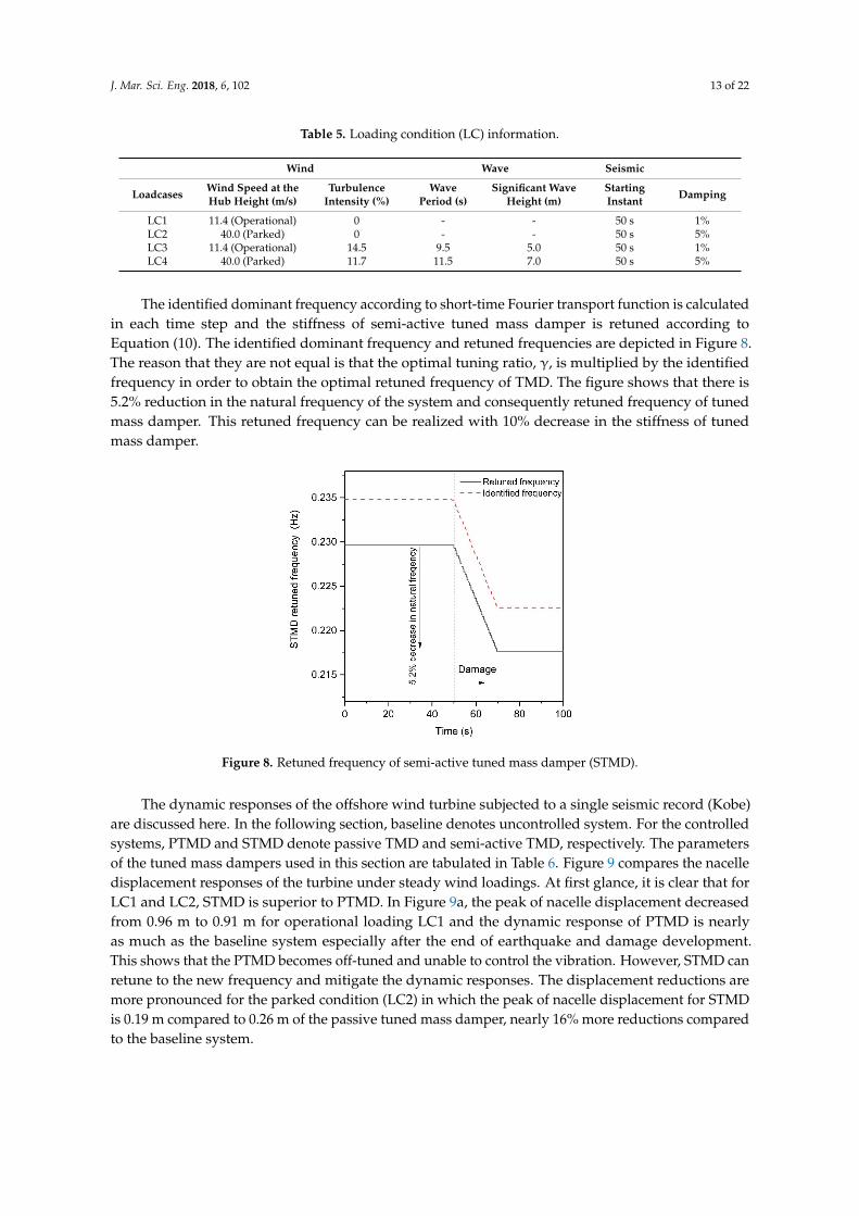
The identified dominant frequency according to short-time Fourier transport function is calculatedin each time step and the stiffness of semi-active tuned mass damper is retuned according toEquation (10). The identified dominant frequency and retuned frequencies are depicted in Figure 8.The reason that they are not equal is that the optimal tuning ratio, γ, is multiplied by the identifiedfrequency in order to obtain the optimal retuned frequency of TMD. The figure shows that there is5.2% reduction in the natural frequency of the system and consequently retuned frequency of tunedmass damper. This retuned frequency can be realized with 10% decrease in the stiffness of tunedmass damper.

J. Mar. Sci. Eng. 2018, 6, x 13 of 22

Table 5. Loading condition (LC) information.

Wind Wave Seismic

Loadcases Wind Speed at the Hub Height (m/s)

Turbulence Intensity (%)

Wave Period (s)

Significant Wave Height

(m)

Starting Instant

Damping

LC1 11.4 (Operational) 0 - - 50 s 1% LC2 40.0 (Parked) 0 - - 50 s 5% LC3 11.4 (Operational) 14.5 9.5 5.0 50 s 1% LC4 40.0 (Parked) 11.7 11.5 7.0 50 s 5%

The identified dominant frequency according to short-time Fourier transport function is calculated in each time step and the stiffness of semi-active tuned mass damper is retuned according to Equation (10). The identified dominant frequency and retuned frequencies are depicted in Figure 8. The reason that they are not equal is that the optimal tuning ratio, γ, is multiplied by the identified frequency in order to obtain the optimal retuned frequency of TMD. The figure shows that there is 5.2% reduction in the natural frequency of the system and consequently retuned frequency of tuned mass damper. This retuned frequency can be realized with 10% decrease in the stiffness of tuned mass damper.

Figure 8. Retuned frequency of semi-active tuned mass damper (STMD).

The dynamic responses of the offshore wind turbine subjected to a single seismic record (Kobe) are discussed here. In the following section, baseline denotes uncontrolled system. For the controlled systems, PTMD and STMD denote passive TMD and semi-active TMD, respectively. The parameters of the tuned mass dampers used in this section are tabulated in Table 6. Figure 9 compares the nacelle displacement responses of the turbine under steady wind loadings. At first glance, it is clear that for LC1 and LC2, STMD is superior to PTMD. In Figure 9a, the peak of nacelle displacement decreased from 0.96 m to 0.91 m for operational loading LC1 and the dynamic response of PTMD is nearly as much as the baseline system especially after the end of earthquake and damage development. This shows that the PTMD becomes off-tuned and unable to control the vibration. However, STMD can retune to the new frequency and mitigate the dynamic responses. The displacement reductions are more pronounced for the parked condition (LC2) in which the peak of nacelle displacement for STMD is 0.19 m compared to 0.26 m of the passive tuned mass damper, nearly 16% more reductions compared to the baseline system.

Figure 8. Retuned frequency of semi-active tuned mass damper (STMD).

The dynamic responses of the offshore wind turbine subjected to a single seismic record (Kobe)are discussed here. In the following section, baseline denotes uncontrolled system. For the controlledsystems, PTMD and STMD denote passive TMD and semi-active TMD, respectively. The parametersof the tuned mass dampers used in this section are tabulated in Table 6. Figure 9 compares the nacelledisplacement responses of the turbine under steady wind loadings. At first glance, it is clear that forLC1 and LC2, STMD is superior to PTMD. In Figure 9a, the peak of nacelle displacement decreasedfrom 0.96 m to 0.91 m for operational loading LC1 and the dynamic response of PTMD is nearlyas much as the baseline system especially after the end of earthquake and damage development.This shows that the PTMD becomes off-tuned and unable to control the vibration. However, STMD canretune to the new frequency and mitigate the dynamic responses. The displacement reductions aremore pronounced for the parked condition (LC2) in which the peak of nacelle displacement for STMDis 0.19 m compared to 0.26 m of the passive tuned mass damper, nearly 16% more reductions comparedto the baseline system.

J. Mar. Sci. Eng. 2018, 6, 102 14 of 22

Table 6. TMD parameters.

Mass (kg) kd (N/m) cd (N/(m/s)) ωd (Hz)

20,000 41,657 10,000 0.229

J. Mar. Sci. Eng. 2018, 6, x 14 of 22

Table 6. TMD parameters.

Mass (kg) kd (N/m) cd (N/(m/s)) ωd (Hz) 20,000 41,657 10,000 0.229

Figure 9. Time history of nacelle displacement under steady wind loading and seismic excitation considering damage development. (a) LC1, (b) LC2. PTMD: passive tuned mass damper.

To scrutinize the energy spectrum of dynamic responses, the power spectral density (PSD) of the nacelle displacements for LC1 and LC2 is obtained and presented in Figure 10. Fast Fourier transformation based on Hamming window is used to capture a smooth PSD curve. Figure 10a indicates that there are two distinct peaks corresponding to the energy of wind loading and turbine frequency (1P) whose frequencies are around zero and 0.2 Hz, respectively. It is clear that the PSD for energy from wind loading (frequencies close to zero) shows negligible changes for PTMD and STMD as these devices are tuned to the first natural frequency of the system. However, a 37% reduction in the peak of the power spectrum for the STMD system can be observed for the turbine frequency (1P). Similarly, power spectral density of the nacelle displacement for LC2 (parked condition) is shown in Figure 10b. Compared to the operational condition (Figure 10a), energy spectrum corresponding to frequency of wind loading (close to zero) has much lower peak due to the fact that in parked condition the turbine absorbs a small portion of wind loading as a result of pitching mechanism in the blades and the energy is concentrated around the frequency range of first natural frequency of structure. This is expected because in the parked condition the vibration of structural modes dominates compared to the operational condition where the vibration due to external excitations dominates. The Figure also indicates that the peak of spectrum for the STMD system is reduced as much as 92% compared to the baseline system (uncontrolled system). However, this percentage reduction is lower for the PTMD with 76% reduction. These reductions for both PTMD and STMD are higher in the parked condition (Figure 10b) compared to the operational condition (Figure 10a) because in the parked conditions the aerodynamic damping is negligible and these structural control devices compensate for low total damping value of the system.

Figure 10. Power spectral density (PSD) of nacelle displacement under steady wind loading and seismic excitation considering damage development. (a) LC1, (b) LC2.

Figure 9. Time history of nacelle displacement under steady wind loading and seismic excitationconsidering damage development. (a) LC1, (b) LC2. PTMD: passive tuned mass damper.

To scrutinize the energy spectrum of dynamic responses, the power spectral density (PSD) ofthe nacelle displacements for LC1 and LC2 is obtained and presented in Figure 10. Fast Fouriertransformation based on Hamming window is used to capture a smooth PSD curve. Figure 10aindicates that there are two distinct peaks corresponding to the energy of wind loading and turbinefrequency (1P) whose frequencies are around zero and 0.2 Hz, respectively. It is clear that the PSD forenergy from wind loading (frequencies close to zero) shows negligible changes for PTMD and STMDas these devices are tuned to the first natural frequency of the system. However, a 37% reduction inthe peak of the power spectrum for the STMD system can be observed for the turbine frequency (1P).Similarly, power spectral density of the nacelle displacement for LC2 (parked condition) is shown inFigure 10b. Compared to the operational condition (Figure 10a), energy spectrum corresponding tofrequency of wind loading (close to zero) has much lower peak due to the fact that in parked conditionthe turbine absorbs a small portion of wind loading as a result of pitching mechanism in the bladesand the energy is concentrated around the frequency range of first natural frequency of structure.This is expected because in the parked condition the vibration of structural modes dominates comparedto the operational condition where the vibration due to external excitations dominates. The Figure alsoindicates that the peak of spectrum for the STMD system is reduced as much as 92% compared to thebaseline system (uncontrolled system). However, this percentage reduction is lower for the PTMDwith 76% reduction. These reductions for both PTMD and STMD are higher in the parked condition(Figure 10b) compared to the operational condition (Figure 10a) because in the parked conditionsthe aerodynamic damping is negligible and these structural control devices compensate for low totaldamping value of the system.

Figure 11 compares the nacelle displacement responses of the turbine under stochastic wave–waveloadings in conjunction with seismic ground motion and damage development (LC3 and LC4). Again itcan be seen that the STMD system shows a better performance in mitigating vibrations and reducingpeak displacements. For example, the peak value of displacement is decreased from 1.5 m of thebaseline system to 1.27 m of the STMD system for the operational condition (LC3), with 15% reduction.This reduction percentage for the PTMD system is lower, as much as only 6%. Therefore, the STMD’seffectiveness in reducing the peak values is more than twice that of the PTMD. For the parked condition(LC4), higher vibration reductions are observed. For example, the peak nacelle displacement reducedfrom 1.91 m to 1.01 m as a result of the implementation of the semi-active tuned mass damper.This means that the semi-active achieves 47% reduction in the peak nacelle displacement.

J. Mar. Sci. Eng. 2018, 6, 102 15 of 22

J. Mar. Sci. Eng. 2018, 6, x 14 of 22

Table 6. TMD parameters.

Mass (kg) kd (N/m) cd (N/(m/s)) ωd (Hz) 20,000 41,657 10,000 0.229

Figure 9. Time history of nacelle displacement under steady wind loading and seismic excitation considering damage development. (a) LC1, (b) LC2. PTMD: passive tuned mass damper.

To scrutinize the energy spectrum of dynamic responses, the power spectral density (PSD) of the nacelle displacements for LC1 and LC2 is obtained and presented in Figure 10. Fast Fourier transformation based on Hamming window is used to capture a smooth PSD curve. Figure 10a indicates that there are two distinct peaks corresponding to the energy of wind loading and turbine frequency (1P) whose frequencies are around zero and 0.2 Hz, respectively. It is clear that the PSD for energy from wind loading (frequencies close to zero) shows negligible changes for PTMD and STMD as these devices are tuned to the first natural frequency of the system. However, a 37% reduction in the peak of the power spectrum for the STMD system can be observed for the turbine frequency (1P). Similarly, power spectral density of the nacelle displacement for LC2 (parked condition) is shown in Figure 10b. Compared to the operational condition (Figure 10a), energy spectrum corresponding to frequency of wind loading (close to zero) has much lower peak due to the fact that in parked condition the turbine absorbs a small portion of wind loading as a result of pitching mechanism in the blades and the energy is concentrated around the frequency range of first natural frequency of structure. This is expected because in the parked condition the vibration of structural modes dominates compared to the operational condition where the vibration due to external excitations dominates. The Figure also indicates that the peak of spectrum for the STMD system is reduced as much as 92% compared to the baseline system (uncontrolled system). However, this percentage reduction is lower for the PTMD with 76% reduction. These reductions for both PTMD and STMD are higher in the parked condition (Figure 10b) compared to the operational condition (Figure 10a) because in the parked conditions the aerodynamic damping is negligible and these structural control devices compensate for low total damping value of the system.

Figure 10. Power spectral density (PSD) of nacelle displacement under steady wind loading and seismic excitation considering damage development. (a) LC1, (b) LC2. Figure 10. Power spectral density (PSD) of nacelle displacement under steady wind loading andseismic excitation considering damage development. (a) LC1, (b) LC2.

J. Mar. Sci. Eng. 2018, 6, x 15 of 22

Figure 11 compares the nacelle displacement responses of the turbine under stochastic wave–wave loadings in conjunction with seismic ground motion and damage development (LC3 and LC4). Again it can be seen that the STMD system shows a better performance in mitigating vibrations and reducing peak displacements. For example, the peak value of displacement is decreased from 1.5 m of the baseline system to 1.27 m of the STMD system for the operational condition (LC3), with 15% reduction. This reduction percentage for the PTMD system is lower, as much as only 6%. Therefore, the STMD’s effectiveness in reducing the peak values is more than twice that of the PTMD. For the parked condition (LC4), higher vibration reductions are observed. For example, the peak nacelle displacement reduced from 1.91 m to 1.01 m as a result of the implementation of the semi-active tuned mass damper. This means that the semi-active achieves 47% reduction in the peak nacelle displacement.

Figure 11. Time history of nacelle displacement under stochastic wind–wave loadings and seismic excitation considering damage development. (a) LC3, (b) LC4.

Looking into power spectral density of the nacelle displacement for LC3 and LC4 in Figure 12, some energy is concentrated around the frequency of 0.1 Hz that corresponds to the energy of wave loadings. Similar to Figure 10, more PSD reduction is observed for parked condition (LC4). However, the difference between the reduction in PSD for PTMD and STMD is less than 10%.

Figure 12. PSD of nacelle displacement under stochastic wind–wave loadings and seismic excitations considering damage development. (a) LC3, (b) LC4.

Figures 13 and 14 show a representative 50 s window time history of the base shear force for steady (LC1 and LC2) and stochastic loadings (LC3 and LC4), respectively. For steady wind loadings (LC1 and LC2), larger base shear is obtained during ground motion and both passive and semi-active TMDs have slight effects on the dynamic responses during the ground motion and damage development. However, the displacements after the damage development are reduced owing to the vibration control devices. For both load cases, STMD is superior to the PTMD. On the other hand, for stochastic loading (Figure 14), changes in the base shear due to tuned mass dampers are insignificant.

Figure 11. Time history of nacelle displacement under stochastic wind–wave loadings and seismicexcitation considering damage development. (a) LC3, (b) LC4.

Looking into power spectral density of the nacelle displacement for LC3 and LC4 in Figure 12,some energy is concentrated around the frequency of 0.1 Hz that corresponds to the energy of waveloadings. Similar to Figure 10, more PSD reduction is observed for parked condition (LC4). However,the difference between the reduction in PSD for PTMD and STMD is less than 10%.

J. Mar. Sci. Eng. 2018, 6, x 15 of 22

Figure 11 compares the nacelle displacement responses of the turbine under stochastic wave–wave loadings in conjunction with seismic ground motion and damage development (LC3 and LC4). Again it can be seen that the STMD system shows a better performance in mitigating vibrations and reducing peak displacements. For example, the peak value of displacement is decreased from 1.5 m of the baseline system to 1.27 m of the STMD system for the operational condition (LC3), with 15% reduction. This reduction percentage for the PTMD system is lower, as much as only 6%. Therefore, the STMD’s effectiveness in reducing the peak values is more than twice that of the PTMD. For the parked condition (LC4), higher vibration reductions are observed. For example, the peak nacelle displacement reduced from 1.91 m to 1.01 m as a result of the implementation of the semi-active tuned mass damper. This means that the semi-active achieves 47% reduction in the peak nacelle displacement.

Figure 11. Time history of nacelle displacement under stochastic wind–wave loadings and seismic excitation considering damage development. (a) LC3, (b) LC4.

Looking into power spectral density of the nacelle displacement for LC3 and LC4 in Figure 12, some energy is concentrated around the frequency of 0.1 Hz that corresponds to the energy of wave loadings. Similar to Figure 10, more PSD reduction is observed for parked condition (LC4). However, the difference between the reduction in PSD for PTMD and STMD is less than 10%.

Figure 12. PSD of nacelle displacement under stochastic wind–wave loadings and seismic excitations considering damage development. (a) LC3, (b) LC4.

Figures 13 and 14 show a representative 50 s window time history of the base shear force for steady (LC1 and LC2) and stochastic loadings (LC3 and LC4), respectively. For steady wind loadings (LC1 and LC2), larger base shear is obtained during ground motion and both passive and semi-active TMDs have slight effects on the dynamic responses during the ground motion and damage development. However, the displacements after the damage development are reduced owing to the vibration control devices. For both load cases, STMD is superior to the PTMD. On the other hand, for stochastic loading (Figure 14), changes in the base shear due to tuned mass dampers are insignificant.

Figure 12. PSD of nacelle displacement under stochastic wind–wave loadings and seismic excitationsconsidering damage development. (a) LC3, (b) LC4.

Figures 13 and 14 show a representative 50 s window time history of the base shear force for steady(LC1 and LC2) and stochastic loadings (LC3 and LC4), respectively. For steady wind loadings (LC1 andLC2), larger base shear is obtained during ground motion and both passive and semi-active TMDshave slight effects on the dynamic responses during the ground motion and damage development.However, the displacements after the damage development are reduced owing to the vibration control

J. Mar. Sci. Eng. 2018, 6, 102 16 of 22

devices. For both load cases, STMD is superior to the PTMD. On the other hand, for stochastic loading(Figure 14), changes in the base shear due to tuned mass dampers are insignificant.J. Mar. Sci. Eng. 2018, 6, x 16 of 22

Figure 13. Time history of fore–aft base shear force under only steady wind loading and seismic excitation considering damage development. (a) LC1, (b) LC2.

Figure 14. Time history of fore–aft base shear force under stochastic wind–wave loadings and seismic excitations considering damage development. (a) LC3, (b) LC4.

Figures 15 and 16 compare the base overturning moment time histories for the controlled and uncontrolled systems. Figure 15 shows that the vibration control devices mitigate the base moment values after the development of damage for steady loading. For load case (LC1), the peak values of the base moment, which occur at 69 s, reduce 10% and 15% when PTMD and STMD are used, respectively. This reduction is higher for the parked condition (LC2), where PTMD and STMD reduce the base moment values up to 43% and 57%, respectively. For stochastic loading (Figure 16), the effect of the vibration control devices is less significant for this single seismic motion record.

Figure 15. Time history of the fore–aft base moment under only steady wind loading and seismic excitation considering damage development. (a) LC1, (b) LC2.

Figure 13. Time history of fore–aft base shear force under only steady wind loading and seismicexcitation considering damage development. (a) LC1, (b) LC2.

J. Mar. Sci. Eng. 2018, 6, x 16 of 22

Figure 13. Time history of fore–aft base shear force under only steady wind loading and seismic excitation considering damage development. (a) LC1, (b) LC2.

Figure 14. Time history of fore–aft base shear force under stochastic wind–wave loadings and seismic excitations considering damage development. (a) LC3, (b) LC4.

Figures 15 and 16 compare the base overturning moment time histories for the controlled and uncontrolled systems. Figure 15 shows that the vibration control devices mitigate the base moment values after the development of damage for steady loading. For load case (LC1), the peak values of the base moment, which occur at 69 s, reduce 10% and 15% when PTMD and STMD are used, respectively. This reduction is higher for the parked condition (LC2), where PTMD and STMD reduce the base moment values up to 43% and 57%, respectively. For stochastic loading (Figure 16), the effect of the vibration control devices is less significant for this single seismic motion record.

Figure 15. Time history of the fore–aft base moment under only steady wind loading and seismic excitation considering damage development. (a) LC1, (b) LC2.

Figure 14. Time history of fore–aft base shear force under stochastic wind–wave loadings and seismicexcitations considering damage development. (a) LC3, (b) LC4.

Figures 15 and 16 compare the base overturning moment time histories for the controlled anduncontrolled systems. Figure 15 shows that the vibration control devices mitigate the base momentvalues after the development of damage for steady loading. For load case (LC1), the peak values of thebase moment, which occur at 69 s, reduce 10% and 15% when PTMD and STMD are used, respectively.This reduction is higher for the parked condition (LC2), where PTMD and STMD reduce the basemoment values up to 43% and 57%, respectively. For stochastic loading (Figure 16), the effect of thevibration control devices is less significant for this single seismic motion record.

J. Mar. Sci. Eng. 2018, 6, x 16 of 22

Figure 13. Time history of fore–aft base shear force under only steady wind loading and seismic excitation considering damage development. (a) LC1, (b) LC2.

Figure 14. Time history of fore–aft base shear force under stochastic wind–wave loadings and seismic excitations considering damage development. (a) LC3, (b) LC4.

Figures 15 and 16 compare the base overturning moment time histories for the controlled and uncontrolled systems. Figure 15 shows that the vibration control devices mitigate the base moment values after the development of damage for steady loading. For load case (LC1), the peak values of the base moment, which occur at 69 s, reduce 10% and 15% when PTMD and STMD are used, respectively. This reduction is higher for the parked condition (LC2), where PTMD and STMD reduce the base moment values up to 43% and 57%, respectively. For stochastic loading (Figure 16), the effect of the vibration control devices is less significant for this single seismic motion record.

Figure 15. Time history of the fore–aft base moment under only steady wind loading and seismic excitation considering damage development. (a) LC1, (b) LC2.

Figure 15. Time history of the fore–aft base moment under only steady wind loading and seismicexcitation considering damage development. (a) LC1, (b) LC2.

J. Mar. Sci. Eng. 2018, 6, 102 17 of 22J. Mar. Sci. Eng. 2018, 6, x 17 of 22

Figure 16. Time history of the fore–aft base moment under stochastic wind–wave loadings and seismic considering damage development. (a) LC3, (b) LC4.

It should be noted that the semi-active tuned mass damper used in this study has both varying stiffness and damping and the combined effect of them is shown in the results. Individual effects of them were also investigated to determine the contribution of each in the response reduction and the results showed that the contribution of each effect individually varies depending on the load cases. However, for all load cases, the contribution of varying damping is larger than the contribution of varying stiffness. For example, the contribution of the varying damping in the response reduction (nacelle deflection) is 57%, whereas the corresponding contribution of varying stiffness is 43%.

4.4. Response to a Seismic Record Set

In this section, more analyses based on a set of ground motion records with different soil and intensity properties as listed in Table 3 are performed and the influences of the structural control devices on the dynamic responses are systematically investigated. Standard deviation and peak values of each time history are taken for the systems equipped with optimal PTMD and STMD with mass ratios ranging between 1% and 4% and compared with the baseline system (uncontrolled system) as the percentage of reduction (improvement). The positive values mean a reduction in the responses which can be defined as the effectiveness of the structural control device. On the other hand, negative values denote increases in the response which means that the vibration control device worsens the vibration performance. The standard deviations and peak values of fore–aft displacements of the nacelle are tracked as they are representative of serviceability and fatigue lifetime of the system, respectively. Then, these values are compared with those of the uncontrolled system (offshore wind turbine without any structural control devices) as the percentage of reduction.

Peak Response Reduction = uncontrolled controlled

uncontrolled

Peak PeakPeak

− (21)

Std Response Reduction = uncontrolled controlled

uncontrolled

Std StdStd

− (22)

in which Peak and Std denote peak and standard deviation of deflections, respectively. Controlled denotes the offshore wind turbine equipped with structural control devices, and Uncontrolled denotes the baseline offshore wind turbine without any vibration control devices. Figure 17a,b illustrates the standard deviation reduction of the nacelle displacement for STMD and PTMD, respectively, for loading condition LC3. For STMD, it is clear that dynamic responses reduce as the mass ratio increases for most ground motions. However, a different trend for PTMD (Figure 17b) is observed in which negative performances are seen for most ground motion records and even increasing the mass ratio of TMD does not improve the performance. This behavior is expected since the passive tuned mass damper is unable to mitigate the vibrations as it becomes off-tune by changing the frequency of the system due to damage development.

Figure 16. Time history of the fore–aft base moment under stochastic wind–wave loadings and seismicconsidering damage development. (a) LC3, (b) LC4.

It should be noted that the semi-active tuned mass damper used in this study has both varyingstiffness and damping and the combined effect of them is shown in the results. Individual effects ofthem were also investigated to determine the contribution of each in the response reduction and theresults showed that the contribution of each effect individually varies depending on the load cases.However, for all load cases, the contribution of varying damping is larger than the contribution ofvarying stiffness. For example, the contribution of the varying damping in the response reduction(nacelle deflection) is 57%, whereas the corresponding contribution of varying stiffness is 43%.

4.4. Response to a Seismic Record Set

In this section, more analyses based on a set of ground motion records with different soil andintensity properties as listed in Table 3 are performed and the influences of the structural controldevices on the dynamic responses are systematically investigated. Standard deviation and peak valuesof each time history are taken for the systems equipped with optimal PTMD and STMD with massratios ranging between 1% and 4% and compared with the baseline system (uncontrolled system) as thepercentage of reduction (improvement). The positive values mean a reduction in the responses whichcan be defined as the effectiveness of the structural control device. On the other hand, negative valuesdenote increases in the response which means that the vibration control device worsens the vibrationperformance. The standard deviations and peak values of fore–aft displacements of the nacelle aretracked as they are representative of serviceability and fatigue lifetime of the system, respectively.Then, these values are compared with those of the uncontrolled system (offshore wind turbine withoutany structural control devices) as the percentage of reduction.

Peak Response Reduction =Peakuncontrolled − Peakcontrolled

Peakuncontrolled(21)

Std Response Reduction =Stduncontrolled − Stdcontrolled

Stduncontrolled(22)

in which Peak and Std denote peak and standard deviation of deflections, respectively. Controlleddenotes the offshore wind turbine equipped with structural control devices, and Uncontrolled denotesthe baseline offshore wind turbine without any vibration control devices. Figure 17a,b illustratesthe standard deviation reduction of the nacelle displacement for STMD and PTMD, respectively,for loading condition LC3. For STMD, it is clear that dynamic responses reduce as the mass ratioincreases for most ground motions. However, a different trend for PTMD (Figure 17b) is observed inwhich negative performances are seen for most ground motion records and even increasing the massratio of TMD does not improve the performance. This behavior is expected since the passive tunedmass damper is unable to mitigate the vibrations as it becomes off-tune by changing the frequency ofthe system due to damage development.

J. Mar. Sci. Eng. 2018, 6, 102 18 of 22J. Mar. Sci. Eng. 2018, 6, x 18 of 22

Figure 17. Standard deviation reduction of fore–aft displacement for LC3 under a set of seismic records. (a) STMD, (b) PTMD.

Figure 17 shows standard deviation reduction for all seismic records for only nacelle displacement under LC3 loading conditions. For the sake of brevity, the dynamic response reductions for all the seismic records are averaged for each loading condition and presented in Figures 18 and 19. The average of reduction percentage in the standard deviation of dynamic responses for all ground motion records for load cases LC3 and LC4 (stochastic wind and wave loading in conjunction with seismic excitation and damage development) is obtained and plotted in Figure 18. Dashed lines correspond to semi-active tuned mass dampers and solid lines are for passive tuned mass dampers. For the operational condition (Figure 18a), the standard deviation of nacelle displacements reduces by 20% for STMD with 1% mass ratio and this reduction percentage increases to 39% by increasing the mass ratio to 4%. On the other hand, the PTMD with 1% mass ratio leads to only 10% standard deviation reduction, half of its STMD counterpart. It is interesting that the performance of PTMD becomes worse when the mass ratio increases up to 4%, resulting in 10% increase in the standard deviation of deflection. This suggests that increasing the mass ratio of PTMD cannot improve its dynamic performance and even it worsens the dynamic performance due to the controller becoming off-tune as well as the reduction in the natural frequency of system as a result of the additional mass of tuned mass damper. From the results shown in Figure 18, it is concluded that a semi-active mass damper with a mass ratio of 1% shows much better performance than a passive tuned mass damper with a mass ratio of 4% for the case when there is a change in natural frequency of the system. This means that STMD with a very low mass ratio is more effective than a PTMD with a large mass ratio. Similar trends can be observed for base shear force and base moment responses; however, it should be noted that base shear force and base moment experience lower dynamic response reduction with the vibration control devices. For example, the standard deviation of the base shear force shows a maximum of 7% reduction for STMD with a mass ratio of 3%. Therefore, it could be concluded that the considered structural control devices have more influence on nacelle displacement and base overturning moments rather than base shear force.

Figure 18. Standard deviation reduction of fore–aft displacement for stochastic wind–wave loadings and seismic excitation. (a) LC3, (b) LC4.

Figure 17. Standard deviation reduction of fore–aft displacement for LC3 under a set of seismic records.(a) STMD, (b) PTMD.

Figure 17 shows standard deviation reduction for all seismic records for only nacelle displacementunder LC3 loading conditions. For the sake of brevity, the dynamic response reductions for allthe seismic records are averaged for each loading condition and presented in Figures 18 and 19.The average of reduction percentage in the standard deviation of dynamic responses for all groundmotion records for load cases LC3 and LC4 (stochastic wind and wave loading in conjunction withseismic excitation and damage development) is obtained and plotted in Figure 18. Dashed linescorrespond to semi-active tuned mass dampers and solid lines are for passive tuned mass dampers.For the operational condition (Figure 18a), the standard deviation of nacelle displacements reducesby 20% for STMD with 1% mass ratio and this reduction percentage increases to 39% by increasingthe mass ratio to 4%. On the other hand, the PTMD with 1% mass ratio leads to only 10% standarddeviation reduction, half of its STMD counterpart. It is interesting that the performance of PTMDbecomes worse when the mass ratio increases up to 4%, resulting in 10% increase in the standarddeviation of deflection. This suggests that increasing the mass ratio of PTMD cannot improve itsdynamic performance and even it worsens the dynamic performance due to the controller becomingoff-tune as well as the reduction in the natural frequency of system as a result of the additionalmass of tuned mass damper. From the results shown in Figure 18, it is concluded that a semi-activemass damper with a mass ratio of 1% shows much better performance than a passive tuned massdamper with a mass ratio of 4% for the case when there is a change in natural frequency of the system.This means that STMD with a very low mass ratio is more effective than a PTMD with a large mass ratio.Similar trends can be observed for base shear force and base moment responses; however, it shouldbe noted that base shear force and base moment experience lower dynamic response reduction withthe vibration control devices. For example, the standard deviation of the base shear force showsa maximum of 7% reduction for STMD with a mass ratio of 3%. Therefore, it could be concludedthat the considered structural control devices have more influence on nacelle displacement and baseoverturning moments rather than base shear force.

J. Mar. Sci. Eng. 2018, 6, x 18 of 22

Figure 17. Standard deviation reduction of fore–aft displacement for LC3 under a set of seismic records. (a) STMD, (b) PTMD.

Figure 17 shows standard deviation reduction for all seismic records for only nacelle displacement under LC3 loading conditions. For the sake of brevity, the dynamic response reductions for all the seismic records are averaged for each loading condition and presented in Figures 18 and 19. The average of reduction percentage in the standard deviation of dynamic responses for all ground motion records for load cases LC3 and LC4 (stochastic wind and wave loading in conjunction with seismic excitation and damage development) is obtained and plotted in Figure 18. Dashed lines correspond to semi-active tuned mass dampers and solid lines are for passive tuned mass dampers. For the operational condition (Figure 18a), the standard deviation of nacelle displacements reduces by 20% for STMD with 1% mass ratio and this reduction percentage increases to 39% by increasing the mass ratio to 4%. On the other hand, the PTMD with 1% mass ratio leads to only 10% standard deviation reduction, half of its STMD counterpart. It is interesting that the performance of PTMD becomes worse when the mass ratio increases up to 4%, resulting in 10% increase in the standard deviation of deflection. This suggests that increasing the mass ratio of PTMD cannot improve its dynamic performance and even it worsens the dynamic performance due to the controller becoming off-tune as well as the reduction in the natural frequency of system as a result of the additional mass of tuned mass damper. From the results shown in Figure 18, it is concluded that a semi-active mass damper with a mass ratio of 1% shows much better performance than a passive tuned mass damper with a mass ratio of 4% for the case when there is a change in natural frequency of the system. This means that STMD with a very low mass ratio is more effective than a PTMD with a large mass ratio. Similar trends can be observed for base shear force and base moment responses; however, it should be noted that base shear force and base moment experience lower dynamic response reduction with the vibration control devices. For example, the standard deviation of the base shear force shows a maximum of 7% reduction for STMD with a mass ratio of 3%. Therefore, it could be concluded that the considered structural control devices have more influence on nacelle displacement and base overturning moments rather than base shear force.

Figure 18. Standard deviation reduction of fore–aft displacement for stochastic wind–wave loadings and seismic excitation. (a) LC3, (b) LC4. Figure 18. Standard deviation reduction of fore–aft displacement for stochastic wind–wave loadingsand seismic excitation. (a) LC3, (b) LC4.

J. Mar. Sci. Eng. 2018, 6, 102 19 of 22

J. Mar. Sci. Eng. 2018, 6, x 19 of 22

Similarly, the average reduction percentage in peak values of dynamic responses for all ground motion records is plotted in Figure 19. Similar trends to the results of standard deviations are observed with some differences. For example, for the operational loading LC3, the reduction in the peak value of the nacelle displacement is 11% for the STMD with a mass ratio of 1% and it increases to 32% with a fourfold increase in the mass ratio. It is worthy to note that the PTMD’s effectiveness in mitigating the peak values of dynamic responses is very low for all the mass ratios. This means that PTMD systems have negative impacts on the peak values, resulting in a deterioration in serviceability of the system. Similar trend for LC4 can be seen in Figure 19b; however, the peak response reductions are higher for STMDs compared to the operational loading.

Figure 19. Peak response reduction of fore–aft displacement for stochastic wind–wave loadings and seismic excitation. (a) LC3, (b) LC4.

Since changes in the natural frequency of the system are inevitable due to various reasons and a number of measurement campaigns in operational wind farms have observed a difference between design natural frequency and real natural frequency, semi-active tuned mass dampers are a better option for massive tuned mass dampers. Therefore, implementation of this kind of vibration control device can mitigate undesired vibrations and reduce the dynamic response, especially the displacements and base overturning moments to a great extent. Consequently, it has the potential to reduce fatigue damages and increase the lifetime of the system, resulting in an improvement in lifecycle of wind turbines and reduction in the cost of energy production. In terms of practicality of implementation, MR dampers can be used as time-variant damping devices and variable stiffness devices can be used in order to change the stiffness of the device.

5. Conclusions

In this paper, a numerical model for an offshore wind turbine controlled by semi-active tuned mass dampers (STMD) subjected to wind, wave, and earthquake excitations considering time-variant damage development are presented. Nonlinear soil–pile interaction is considered. Short-time Fourier transform (STFT) is utilized to identify the changes in the natural frequency of the system and to retune the semi-active tuned mass damper. Time-variant stiffness and damping of STMD are modified in each time step according to a vibration control algorithm based on short-time Fourier transform. Numerical analyses are carried out for operational and nonoperational conditions to investigate the performance of STMD compared to the PTMD under multihazards. Dynamic responses for a single earthquake record as well as a set of earthquake records are presented. The results show that STMDs perform significantly better than PTMDs, especially when there is a change in natural frequency of the system. A semi-active mass damper with a mass ratio of 1% shows much better performance than a passive tuned mass damper with a mass ratio of 4%. A semi-active tuned mass damper with a mass ratio of 2% can reduce the standard deviation of the displacement and base overturning moment up to 20% and 16%, respectively. However, its passive counterpart increases the dynamic responses. This significant difference between the performances of the passive and semi-active devices is for the case when the natural frequency is shifted by up to only 5% and is even higher for the case with higher frequency changes. The results highlight the significance of implementation

Figure 19. Peak response reduction of fore–aft displacement for stochastic wind–wave loadings andseismic excitation. (a) LC3, (b) LC4.

Similarly, the average reduction percentage in peak values of dynamic responses for all groundmotion records is plotted in Figure 19. Similar trends to the results of standard deviations are observedwith some differences. For example, for the operational loading LC3, the reduction in the peak valueof the nacelle displacement is 11% for the STMD with a mass ratio of 1% and it increases to 32% with afourfold increase in the mass ratio. It is worthy to note that the PTMD’s effectiveness in mitigating thepeak values of dynamic responses is very low for all the mass ratios. This means that PTMD systemshave negative impacts on the peak values, resulting in a deterioration in serviceability of the system.Similar trend for LC4 can be seen in Figure 19b; however, the peak response reductions are higher forSTMDs compared to the operational loading.

Since changes in the natural frequency of the system are inevitable due to various reasonsand a number of measurement campaigns in operational wind farms have observed a differencebetween design natural frequency and real natural frequency, semi-active tuned mass dampers are abetter option for massive tuned mass dampers. Therefore, implementation of this kind of vibrationcontrol device can mitigate undesired vibrations and reduce the dynamic response, especially thedisplacements and base overturning moments to a great extent. Consequently, it has the potentialto reduce fatigue damages and increase the lifetime of the system, resulting in an improvement inlifecycle of wind turbines and reduction in the cost of energy production. In terms of practicality ofimplementation, MR dampers can be used as time-variant damping devices and variable stiffnessdevices can be used in order to change the stiffness of the device.

5. Conclusions

In this paper, a numerical model for an offshore wind turbine controlled by semi-active tunedmass dampers (STMD) subjected to wind, wave, and earthquake excitations considering time-variantdamage development are presented. Nonlinear soil–pile interaction is considered. Short-time Fouriertransform (STFT) is utilized to identify the changes in the natural frequency of the system and to retunethe semi-active tuned mass damper. Time-variant stiffness and damping of STMD are modified in eachtime step according to a vibration control algorithm based on short-time Fourier transform. Numericalanalyses are carried out for operational and nonoperational conditions to investigate the performanceof STMD compared to the PTMD under multihazards. Dynamic responses for a single earthquakerecord as well as a set of earthquake records are presented. The results show that STMDs performsignificantly better than PTMDs, especially when there is a change in natural frequency of the system.A semi-active mass damper with a mass ratio of 1% shows much better performance than a passivetuned mass damper with a mass ratio of 4%. A semi-active tuned mass damper with a mass ratio of 2%can reduce the standard deviation of the displacement and base overturning moment up to 20% and16%, respectively. However, its passive counterpart increases the dynamic responses. This significantdifference between the performances of the passive and semi-active devices is for the case when thenatural frequency is shifted by up to only 5% and is even higher for the case with higher frequency

J. Mar. Sci. Eng. 2018, 6, 102 20 of 22

changes. The results highlight the significance of implementation of a semi-active tuned mass damperfor offshore wind turbines which are subjected to varying natural frequency due to gradual or suddendamage development. To implement the aforementioned structural control devices in the design ofoffshore wind turbines, more comprehensive studies with a focus on the experimental investigationsand practicalities of these devices are needed. Furthermore, the maintenance requirements of thesedevices should be investigated in the scope of total maintenance regime of the offshore wind turbine.

Author Contributions: A.H. and E.O. conceived and designed the simulations. A.H. developed the simulationtool. A.H. and E.O. analyzed the data and wrote the paper.

Acknowledgments: This research was made possible by a Ph.D. scholarship from the University ofStrathclyde scholarship.

Conflicts of Interest: The authors declare no conflict of interest.

References

1. Symans, M.D.; Constantinou, M.C. Semi-active control systems for seismic protection of structures:A state-of-the-art review. Eng. Struct. 1999, 21, 469–487. [CrossRef]

2. Chen, J.-L.; Georgakis, C.T. Spherical tuned liquid damper for vibration control in wind turbines.J. Vib. Control. 2013, 21, 1875–1885. [CrossRef]

3. Housner, G.W.; Bergman, L.A.; Caughey, T.K.; Chassiakos, A.G.; Claus, R.O.; Masri, S.F.; Skelton, R.E.;Soong, T.T.; Spencer, B.F.; Yao, J.T.P. Structural Control: Past, Present, and Future. J. Eng. Mech. 1997, 123,897–971. [CrossRef]

4. Soong, T.T.; Spencer, B.F. Supplemental energy dissipation: state-of-the-art and state-of-the-practice.Eng. Struct. 2002, 24, 243–259. [CrossRef]

5. Enevoldsen, I.; Mørk, K.J. Effects of a Vibration Mass Damper in a Wind Turbine Tower*. Mech. Struct. Mach.1996, 24, 155–187. [CrossRef]

6. Murtagh, P.J.; Ghosh, A.; Basu, B.; Broderick, B.M. Passive control of wind turbine vibrations includingblade/tower interaction and rotationally sampled turbulence. Wind Energy 2008, 11, 305–317. [CrossRef]

7. Colwell, S.; Basu, B. Tuned liquid column dampers in offshore wind turbines for structural control. Eng. Struct.2009, 31, 358–368. [CrossRef]

8. Stewart, G.M.; Lackner, M.A. The impact of passive tuned mass dampers and wind–wave misalignment onoffshore wind turbine loads. Eng. Struct. 2014, 73, 54–61. [CrossRef]

9. Stewart, G.; Lackner, M. Offshore wind turbine load reduction employing optimal passive tuned massdamping systems. IEEE Transact. Control. Syst. Technol. 2013, 21, 1090–1104. [CrossRef]

10. Dinh, V.N.; Basu, B. Passive control of floating offshore wind turbine nacelle and spar vibrations by multipletuned mass dampers. Struct. Control. Health Monit. 2014, 22, 152–176. [CrossRef]

11. Lackner, M.; Rotea, M.; Saheba, R. Active structural control of offshore wind turbines. In Proceedings ofthe 48th AIAA Aerospace Sciences Meeting Including the New Horizons Forum and Aerospace Exposition,Orlando, FL, USA, 4–7 January 2010.

12. Fitzgerald, B.; Basu, B.; Nielsen, S.R.K. Active tuned mass dampers for control of in-plane vibrations of windturbine blades. Struct. Control. Health Monit. 2013, 20, 1377–1396. [CrossRef]

13. Fitzgerald, B.; Basu, B. Active tuned mass damper control of wind turbine nacelle/tower vibrations withdamaged foundations. Key Eng. Mater. 2013, 569–570, 660–667. [CrossRef]

14. Staino, A.; Basu, B. Dynamics and control of vibrations in wind turbines with variable rotor speed. Eng. Struct.2013, 56, 58–67. [CrossRef]

15. Krenk, S.; Svendsen, M.N.; Høgsberg, J. Resonant vibration control of three-bladed wind turbine rotors.AIAA J. 2012, 50, 148–161. [CrossRef]

16. Maldonado, V.; Boucher, M.; Ostman, R.; Amitay, M. Active vibration control of a wind turbine blade usingsynthetic jets. Int. J. Flow Control. 2009, 1, 227–238. [CrossRef]

17. Fitzgerald, B.; Basu, B. Cable connected active tuned mass dampers for control of in-plane vibrations of windturbine blades. J. Sound Vib. 2014, 333, 5980–6004. [CrossRef]

18. Kim, S.-M.; Wang, S.; Brennan, M.J. Optimal and robust modal control of a flexible structure using an activedynamic vibration absorber. Smart Mater. Struct. 2011, 20, 045003. [CrossRef]

J. Mar. Sci. Eng. 2018, 6, 102 21 of 22

19. Yalla, S.K.; Kareem, A.; Kantor, J.C. Semi-active tuned liquid column dampers for vibration control ofstructures. Eng. Struct. 2001, 23, 1469–1479. [CrossRef]

20. Hrovat, D.; Barak, P.; Rabins, M. Semi-active versus passive or active tuned mass dampers for structuralcontrol. J. Eng. Mech. 1983, 109, 691–705. [CrossRef]

21. Sun, C.; Nagarajaiah, S. Study on semi-active tuned mass damper with variable damping and stiffness underseismic excitations. Struct. Control. Health Monit. 2013, 21, 890–906. [CrossRef]

22. Karnopp, D.; Crosby, M.J.; Harwood, R. Vibration control using semi-active force generators. J. Eng. Ind.1974, 96, 619–626. [CrossRef]

23. Nagarajaiah, S.; Sonmez, E. Structures with semiactive variable stiffness single/multiple tuned mass dampers.J. Struct. Eng. 2007, 133, 67–77. [CrossRef]

24. Kirkegaard, P.H.; Nielsen, S.R.K.; Poulsen, B.L.; Andersen, J.; Pedersen, L.H.; Pedersen, B.J. Semiactivevibration control of a wind turbine tower using an MR damper. In Proceedings of the Fifth EuropeanConference on Structural Dynamics, Munich, Germany, 2–5 September 2002.

25. Karimi, H.R.; Zapateiro, M.; Luo, N. Semiactive vibration control of offshore wind turbine towers with tunedliquid column dampers using H output feedback control. In Proceedings of the 2010 IEEE InternationalConference on Control Applications, Yokohama, Japan, 8–10 September 2010.

26. Arrigan, J.; Pakrashi, V.; Basu, B.; Nagarajaiah, S. Control of flapwise vibrations in wind turbine blades usingsemi-active tuned mass dampers. Struct. Control. Health Monit. 2010, 18, 840–851. [CrossRef]

27. Weber, F. Dynamic characteristics of controlled MR-STMDs of Wolgograd Bridge. Smart Mater. Struct. 2013,22, 095008. [CrossRef]

28. Sonmez, E.; Nagarajaiah, S.; Sun, C.; Basu, B. A study on semi-active Tuned Liquid Column Dampers(sTLCDs) for structural response reduction under random excitations. J. Sound Vib. 2016, 362, 1–15.[CrossRef]

29. Sun, C. Semi-active control of monopile offshore wind turbines under multi-hazards. Mech. Syst. Signal Proc.2018, 99, 285–305. [CrossRef]

30. Song, B.; Yi, Y.; Wu, J.C. Study on Seismic Dynamic Response of Offshore Wind Turbine Tower with MonopileFoundation Based on M Method. Adv. Mater. Res. 2013, 663, 686–691. [CrossRef]

31. Abé, M.; Igusa, T. Semi-Active Dynamic Vibration Absorbers For Controlling Transient Response.J. Sound Vib. 1996, 198, 547–569. [CrossRef]

32. Sun, C. Mitigation of offshore wind turbine responses under wind and wave loading: Considering soileffects and damage. Struct. Control Health Monit. 2018, 25, 1–22. [CrossRef]

33. Sadek, F.; Mohraz, B.; Taylor, A.W.; Chung, R.M. A method of estimating the parameters of tuned massdampers for seismic applications. Earthq. Eng. Struct. Dyn. 1997, 26, 617–636. [CrossRef]

34. Jonkman, J.; Butterfield, S.; Musial, W.; Scott, G. Definition of a 5-MW Reference Wind Turbine for Offshore SystemDevelopment; Office of Energy Efficiency and Renewable Energy: Washington, DC, USA, 2009; TechnicalReport No. NREL/TP-500-38060.

35. Jonkman, J.; Musial, W. Offshore code comparison collaboration (OC3) for IEA task 23 offshore windtechnology and deployment. Off. Sci. Technol. Inf. Technol. Rep. 2010, 303, 275–3000.

36. American Petroleum Institute (API). RP 2A-WSD: Recommended Practice for Planning, Designing and ConstructingFixed Offshore Platforms Working Stress Design; API Publishing Services: Short Hills, NJ, USA, 2000.

37. DNV. DNV-OS-J101 Design of Offshore Wind Turbine Structures; DNV: Oslo, Norway, 2004.38. Kaimal, J.; Wyngaard, J.; Izumi, Y.; Cote, O. Spectral characteristics of surface-layer turbulence. Q. J. R.

Meteorol. Soc. 1972, 98, 563–589. [CrossRef]39. Jonkman, B.J. TurbSim user’s guide: version 1.50. Nrel Rep. Natl Renew. Energy Lab. 2009, 7, 58.40. Jonkman, J.M.; Buhl, M.L. SciTech Connect.: FAST User’s Guide-Updated August 2005; Technical Report No.

NREL/TP-500-38230; SciTech: Perth, Australia, 2005.41. DNV. DNV-RP-C205: Environmental conditions and environmental loads; DNV: Oslo, Norway, 2010; pp. 9–123.42. Hasselmann, K. Measurements of wind-wave growth and swell decay during the Joint North Sea Wave

Project (JONSWAP). Dtsch.hydrogr.z 1973, 12, 1–95.43. Chiou, B.; Darragh, R.; Gregor, N.; Silva, W. NGA Project Strong-Motion Database. Earthq. Spectr. 2008, 24,

23–44. [CrossRef]44. Doherty, P.; Gavin, K. Laterally loaded monopile design for offshore wind farms. Proc. Inst. Civ. Eng. Energy

2012, 165, 7–17. [CrossRef]

J. Mar. Sci. Eng. 2018, 6, 102 22 of 22

45. Kim, D.H.; Lee, S.G.; Lee, I.K. Seismic fragility analysis of 5 MW offshore wind turbine. Renew. Energy 2014,65, 250–256. [CrossRef]

46. Achmus, M.; Kuo, Y.-S.; Abdel-Rahman, K. Behavior of monopile foundations under cyclic lateral load.Comput. Geotech. 2009, 36, 725–735. [CrossRef]

47. International Electrotechnical Commission. IEC 61400-1: Wind Turbines Part 1: Design Requirements, 3rd ed.;IEC: Geneva, Switzerland, 2005.

© 2018 by the authors. Licensee MDPI, Basel, Switzerland. This article is an open accessarticle distributed under the terms and conditions of the Creative Commons Attribution(CC BY) license (http://creativecommons.org/licenses/by/4.0/).