Semi Global Boundary Detection

Roy Josef Jevnisek, Shai AvidanTel-Aviv University

AbstractSemi Global Boundary Detection (SGBD) breaks the image into scan lines inmultiple orientations, segments each one independently, and combines the resultsinto a final probabilistic 2D boundary map.

The reason we break the image into scan lines is that they are a mid-levelimage representation that captures more information than a local patch. Luckily,scan lines are 1D signals that can be optimally segmented using dynamic pro-gramming, and we make the assumption that the border pixels between segmentsare boundary pixels in the image.

This leads to a simple and efficient algorithm for boundary detection. Theentire algorithm requires little parameter tuning, works well across different datasets and modalities, and produces sharp boundaries. We report results on severalbenchmarks that include both color and depth.

Keywords: Edge / Boundary Detection, Semi Global Matching

1. Introduction

The goal of this work is to accurately detect and localize boundaries in naturalscenes using image measurements along scan lines. We use Dynamic Program-ming (DP) to find an optimal segmentation for each scan line and take the bound-aries between these 1D segments to determine boundary pixels in the image.

Boundary pixels can be recovered either locally or globally. Edge detectionalgorithms are local in the sense that they determine if a pixel is a boundary pixelbased on a local patch around it. Global methods, on the other hand, partition theimage into regions based on global considerations. The boundary pixels then aretaken to be the boundaries between regions. The two approaches can be combinedwith local methods providing important cues to a global algorithm.

We propose a mid-level image representation that is based on scan lines indifferent directions (e.g., rows, columns). Scan lines are not local, because they

Preprint submitted to Computer Vision and Image Understanding June 26, 2016

extend beyond a local patch. On the other hand, they are not global, because ascan line does not span the whole image. The reason we use scan lines is thatthey are a 1D signal and there are efficient and optimal algorithms for segmentingthem.

Interestingly, a similar approach works quite well in stereo. There, SemiGlobal Matching (SGM) [1] solves stereo matching by breaking the image intomultiple scan lines in different directions and finding an optimal stereo matchingfor each scan line independently. The results from all scan lines are later combinedto give the final stereo matching solution. SGM-based algorithms are consistentlyranked at the top of various stereo benchmarks such as the Middlebury data set[2] and the KITTI dataset [3].

Our algorithm, termed Semi Global Boundary Detection (SGBD), breaks animage into multiple scan lines in different directions. It then segments each scanline multiple times with different number of segments per scan line and differentfeature channels. Each such segmentation give rise to boundary pixels and be-cause we collect statistics of each segment within a scan line we can determinethe strength of boundary pixels. The results are then aggregated to obtain a finalprobability map.

The proposed algorithm enjoys a number of favorable features. It requirestuning just a small number of parameters and we tune them only once on the theBSDS500 training set. Once tuned, it performs consistently well across a widerange of image data sets and imaging conditions. This includes indoor as well asoutdoor images, RGB as well as depth images and clean as well as noisy images.This is an important quality of the algorithm because we do not know who isgoing to use it and on what type of images. Finally, the algorithm is simple toimplement, quite fast in practice, and can be easily made to run in parallel on aGPU (The source code will be released).

2. Background

The literature on edge detection is vast and will not be covered here. A popularand early edge detector that is still in use today is the Canny edge detector [4] thatdetects a peak in gradient magnitude in the direction normal to the edge.

A trend in recent years, though, is to learn edge detectors. Martin et al. learn todetect natural image boundaries using local brightness, color and texture cues [5].Dollar et al. use a boosted classifier to classify each pixel based on its surround-ing patch [6]. Mairal et al. use discriminative sparse image models to learn classspecific edge detectors [7]. Ren and Bo learned sparse codes of patch gradients

2

[8]. Recently, Dollar and Zitnick [9] used structured forest for fast edge detec-tion. Leordeanu et al. [10] proposed a closed-form solution to the generalizedboundary detection problem. They assume that boundaries often coincide acrossmultiple channels and fit them with a linear model. This is reduced to solving aneigenvector problem.

These different edge detectors fit the framework of Arbelaez et al. [11] thatalso proposed a contour detection based on multiple local cues. They furthershowed how the output of any contour detection can be fed into a globalizationframework based on spectral clustering that leads to an automatically generatedhierarchical segmentation.

Recently, Isola et al. [12] introduced a crisp boundary detection algorithmthat relies on pointwise mutual information. In particular, they observe that pixelsbelonging to the same object exhibit higher statistical dependencies than pixelsbelonging to different objects. These dependencies are used as local cues forspectral clustering [11].

Andres et al. [13] treat the problem of image segmentation as a multi-cutproblem that can be solved using Integer Linear Programming (ILP) with an ex-ponential number of constraints. However, they can find the violating constraintsin polynomial time and add them iteratively. This gives a practical solution to themulticut problem which is NP-hard.

Our algorithm is inspired by the work of Hirschmuller on Semi Global Match-ing (SGM) [1]. He used SGM to solve stereo matching by breaking the image intomultiple scanlines in different directions and finding an optimal stereo matchingfor each scanline independently. The results from all scanlines are later combinedto give the final stereo matching solution.

SGM uses Dynamic Programming to find the optimal disparity assignment perscanline. We use Dynamic Programming as well, but use it for segmentation andnot labeling. In fact, our work closely follows the original work of Bellman thatused Dynamic Programming for a piecewise linear approximation of curves [14].

It is instructive to relate our work on segmenting scan lines to work on imagesegmentation using graph cuts. For example, Zabih and Kolmogorov [15] pro-posed an EM procedure for unsupervised image segmentation. The M step dividesthe pixels into categories (without enforcing spatial coherency) using a standardclustering technique (i.e., k-means). The E step runs graph-cut [16] to segmentthe image into spatially coherent regions based on the current category estimates.The advantage of such an approach is that it works on the entire image at once.On the downside, observe that it combines two non-optimal steps (graph-cuts andk-means). In fact, this is also done in the case of interactive image segmentation

3

0 50 100 150 200 250 3000 2 4 6 8 10 12 14 16 18 20

0

0.05

0.1

0.15

0.2

0.25

(a) (b) (c)

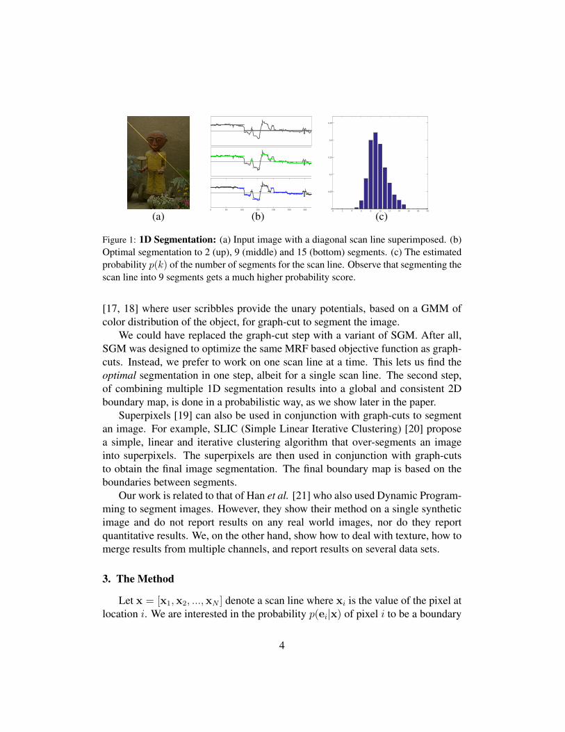
Figure 1: 1D Segmentation: (a) Input image with a diagonal scan line superimposed. (b)Optimal segmentation to 2 (up), 9 (middle) and 15 (bottom) segments. (c) The estimatedprobability p(k) of the number of segments for the scan line. Observe that segmenting thescan line into 9 segments gets a much higher probability score.

[17, 18] where user scribbles provide the unary potentials, based on a GMM ofcolor distribution of the object, for graph-cut to segment the image.

We could have replaced the graph-cut step with a variant of SGM. After all,SGM was designed to optimize the same MRF based objective function as graph-cuts. Instead, we prefer to work on one scan line at a time. This lets us find theoptimal segmentation in one step, albeit for a single scan line. The second step,of combining multiple 1D segmentation results into a global and consistent 2Dboundary map, is done in a probabilistic way, as we show later in the paper.

Superpixels [19] can also be used in conjunction with graph-cuts to segmentan image. For example, SLIC (Simple Linear Iterative Clustering) [20] proposea simple, linear and iterative clustering algorithm that over-segments an imageinto superpixels. The superpixels are then used in conjunction with graph-cutsto obtain the final image segmentation. The final boundary map is based on theboundaries between segments.

Our work is related to that of Han et al. [21] who also used Dynamic Program-ming to segment images. However, they show their method on a single syntheticimage and do not report results on any real world images, nor do they reportquantitative results. We, on the other hand, show how to deal with texture, how tomerge results from multiple channels, and report results on several data sets.

3. The Method

Let x = [x1,x2, ...,xN ] denote a scan line where xi is the value of the pixel atlocation i. We are interested in the probability p(ei|x) of pixel i to be a boundary

4

pixel between two segments, when segmenting the entire scan line x into k seg-ments. Since we don’t know the number of segments k ahead of time we applythe law of total probability and obtain:

p(ei|x) =K∑k=1

p(ei|x, k)p(k|x). (1)

In words, the probability p(ei|x) is marginalized over all possible segmen-tations of x into k segments. Clearly, there are many ways to segment x intok segments and we make the simplifying assumption that only the optimal seg-mentation matters. We show how to find the optimal segmentation in section 3.1.Since k is not given ahead of time we show how to compute p(k|x) using theprincipal of Minimum Description Length (MDL) in section 3.2. In section 3.3we show how to estimate p(ei|x, k) which is the local probability of a pixel to bean edge pixel, given that x is segmented into k segments.

3.1. Optimal Segmentation of 1D SignalsWe wish to find an optimal segmentation of x into k segments, where each seg-

ment is represented by a model (e.g., constant, linear, etc...). To do so, define an er-ror function err(i, j) that determines how well the model approximates the pointsxi, · · · ,xj . Let OPTk(n) denote the optimal error of segmenting [x1,x2, ...,xn]into k segments. We are interested in OPTK(N) and can find it using the follow-ing recursive equation:

OPTk(N) = min1≤m≤N−1

{OPTk−1(m) + err(m+ 1, N)}

With the initial condition OPT1(m) = err(1,m). This can be solved using dy-namic programming. By backtracking OPTK(N) we can find the set of transi-tions (i.e., edge pixels) as well.

The complexity of the algorithm isO(N3) because we need to compute err(i, j)for O(N2) pairs and each such operation takes O(N). This can be reduced toO(N2) by using an integral scan line (i.e., a 1D integral image). For an imageof size N × N pixels, the overall complexity of the algorithm is O(NKN2) =O(N3), where N is the length of the scan line (say, width or height of the image)and K is the maximum number of segments per scan line (K is a small constant).

5

3.2. Estimating Number of SegmentsThe optimal segmentation algorithm described above assumes the number of

segments,K, is known. This is not the case in practice. We cannot choose aK thatminimizes the segmentation error because the error is monotonically decreasingas K increases. Instead, we use the Minimal Descriptive Length (MDL) principlethat penalizes the model as the number of parameters (i.e., segments) increases.It was shown in [21] that the MDL factor for a piecewise polynomial functionwith degree P and white additive Gaussian noise is proportional to KPln(N).Therefore, we define the MDL error for k to be:

MDLE(k) = OPTk(N) + λkP ln(N) (2)

where λ is a regularization weight balancing the measured error with the numberof segments used. Minimizing (2) implies that there is only one correct value fork. A better alternative is to estimate the probability distribution function (pdf) ofk. To do so, we normalize it into a probability:

p(k|x) = 1

Z· exp

{−MDLE(k)−MDLEmin

σ2

}(3)

Where MDLEmin is the minimal value of (2) over all k, Z is a factor that nor-malizes the distribution p(k) and σ2 is a tunable parameter that controls the spreadof p(k). This gives us the probability of segmenting x into k segments. Figure 1illustrates this. It shows an image with a diagonal scan line superimposed on it.Next to it we show the results of optimally segmenting this 1D line into differ-ent numbers of segments. As can be seen, p(k), the probability of the number ofsegments, for this scan line peaks at k = 9.

3.3. Estimating Local Edge StrengthOnce we segment x into k segments we need to assign a probability to each

boundary pixel found by that segmentation. For example, we can set

p(ei|x, k) = 1k(xi) (4)

where 1k(xi) is an indicator function that equals 1 if xi is a transition pixel whenoptimally segmenting x into k segments and zero otherwise. This means that alledge pixels found for a particular value k have the same probability. Clearly, thisis not true in practice and we must augment 1k(xi) with some local edge esti-mation. For example, we can approximate each segment with its mean and take

6

the difference of the means to the left and right of the edge pixel to measure localedge strength. This did not work well in practice. The reason that the difference ofmeans failed is that it falsely enhanced edges inside textured areas, where bound-aries do not exist. In also falsely punished edges between two textures that arevery different but have similar means.

This is why we introduce texture as a way to measure edge strength. Specif-ically, we calculate a histogram of textons for every segment. We then take thelocal edge strength to be the chi-square distance between the texton histograms tothe right and to the left of the boundary. Formally:

p(ei|x, k) = 1k(xi)χ2(hL,xi

, hR,xi) (5)

where hL,xiand hR,xi

are the texton histograms to the left and right of the edgepixel xi, respectively.

We calculate the texton histograms in a method similar to [11]. Given an inputimage, we convert it to Lab space and work on the L channel. We convolve the Lchannel with 16 Gaussian derivative filters, then cluster the 16D vectors into 32prototype textons using k-means and assign each pixel to the closest prototype.

It is worth comparing the approach we take to the one taken by Arbelaez et al.[11]. There, edge pixels are first detected using a fixed scale local operator andthen merged into a global solution using normalized cuts. Here, on the other hand,edge pixels are first detected in a semi-global manner. Then we estimate the localedge strength at those points. This allows us to use adaptive scale. For each edgepixel we look at the segments to its left and right, extract a histogram of textonsand measure the chi-squared distance between the two histograms.

4. The Algorithm

Section 3 described the method we use for a single scanline. Here we providethe overall algorithm. It consists of the following steps:

1. Semi-Global Smoothing the image.2. Running the 1D method on each scan line.3. Merging the 1D results to produce a 2D edge map.

As an optional post-processing step we run the Ultrametric contour map algorithm[11]. Algorithm 1 gives the pseudo-code.

7

4.1. Semi-Global SmoothingWe work in Lab space and observe noticeable jpeg compression artifacts, esp-

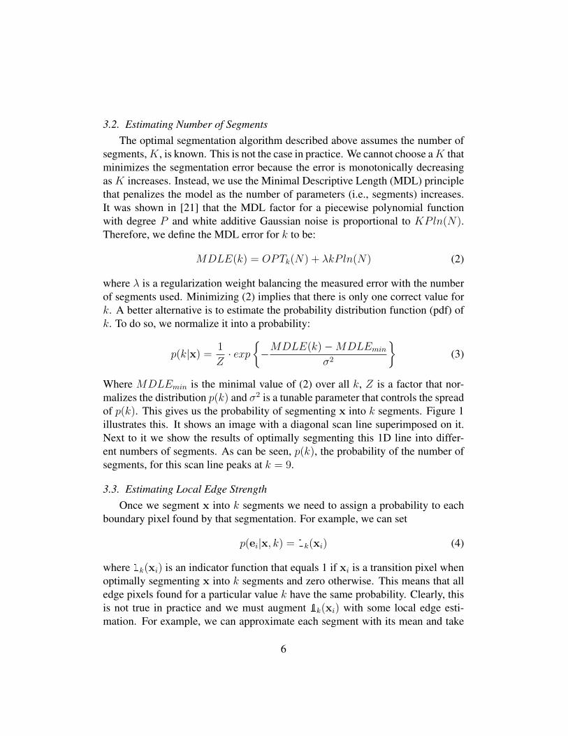
cially in the a and b channels, that cause multiple spurious edges. Smoothing theimage with a median, Gaussian or bilateral filter did not eliminate these artifacts.Therefore, we perform semi-global smoothing. Figure 2 illustrates semi-globalsmoothing on the L, a and b channels of an image.

Semi-global smoothing relies on 1D segmentation to determine the spatialextent of smoothing. Specifically, let xi ∈ sk(j) denote that pixel xi belongs tothe j-th segment when segmenting x into k segments. Then the smoothed valueof xi is set to:

xSmoothi =

∑k

p(k|x) · µsk(j) (6)

Where µsk(j) is the mean of segment sk(j). This smoothing operation is quitestrong, so for the a and b channels we average it with the original channels. TheL channel was not smoothed. In addition, we normalize the mean and variance ofthe image to a global mean and variance that was computed once on the BSDS500training set.

Once we have smoothed the a and b channel, and have normalized all threechannels for mean and variance, we run our method on each scan line in eachchannel in each direction.

4.2. Merging 1D Results to 2D Edge MapAfter running our method on all scan lines we end up with four 2D proba-

bility maps per channel. These maps are the result of running the algorithm indifferent directions (i.e., rows, columns and both diagonals). Each map indicatesthe probability of a pixel to belong to a boundary (i.e., edge) that is in a directionperpendicular to the scan line.

We merge the edge maps in each direction by taking the maximum acrossthe different channels, as each channel reflects different properties. This gives usfour edge maps, one per direction that encodes edge information from all chan-nels. Finally, we determine the orientation of each boundary pixel by projectingthe four maps onto several orientations and picking the one that maximizes theircombination.

As a final step we feed our edge maps to the Ultrametric contour map al-gorithm [11]. As an input to the oriented watershed transform we provide asmoothed version of the four probability maps that we calculated. In addition[11]’s code expects 8-channels, so we averaged the results of consecutive angles,0◦ with 45◦, 45◦ with 90◦ and so on, to extend the 4 directions into 8. A pseudo-code of the algorithm is given in Algorithm 1.

8

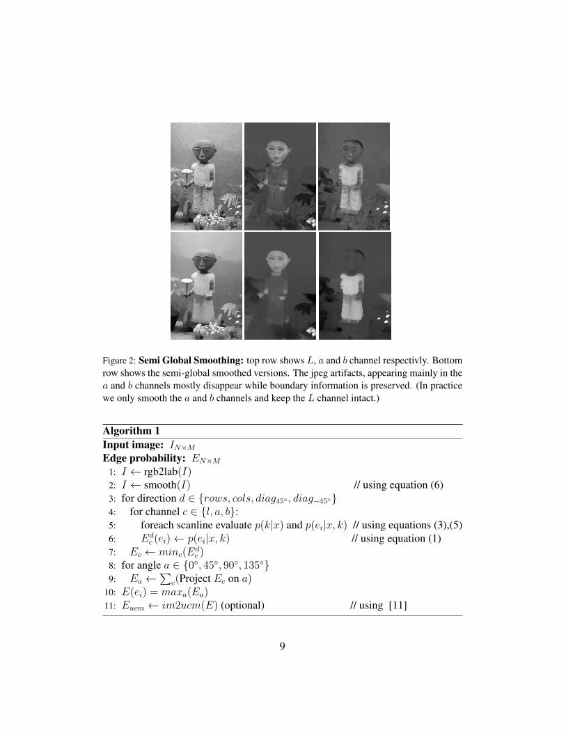
Figure 2: Semi Global Smoothing: top row shows L, a and b channel respectivly. Bottomrow shows the semi-global smoothed versions. The jpeg artifacts, appearing mainly in thea and b channels mostly disappear while boundary information is preserved. (In practicewe only smooth the a and b channels and keep the L channel intact.)

Algorithm 1Input image: IN×M

Edge probability: EN×M

1: I ← rgb2lab(I)2: I ← smooth(I) // using equation (6)3: for direction d ∈ {rows, cols, diag45◦ , diag−45◦}4: for channel c ∈ {l, a, b}:5: foreach scanline evaluate p(k|x) and p(ei|x, k) // using equations (3),(5)6: Ed

c (ei)← p(ei|x, k) // using equation (1)7: Ec ← minc(E

dc )

8: for angle a ∈ {0◦, 45◦, 90◦, 135◦}9: Ea ←

∑c(Project Ec on a)

10: E(ei) = maxa(Ea)11: Eucm ← im2ucm(E) (optional) // using [11]

9

5. Results

We report results on a number of datasets. The first is the original BerkeleySegmentation Data Set (BSDS300), the second is the new and larger BSDS500,and the third is the NYU RGBD data set. On the NYU dataset we report resultson the RGB component as well as the depth component, in addition to resultson RGBD. This dataset was used by Ren and Bo [8] to evaluate edge detectionusing RGB or RGBD images. Their algorithm requires training and they use a60%/40% training/testing split. We don’t use the training set and report resultson the test set only. We also demonstrate the tolerance of the algorithm to noise,and perform an experiment on BSDS500 images that are corrupted with whiteGaussian noise.

All experiments were carried out with the same parameters. The parameterswere tuned using the 200 training set images of the BSDS500 data set. Oncetuned, these parameters are fixed in all the experiments reported here. The param-eters that needs to be tuned are γ, the tradeoff between segmentation error and theMDL factor, and σ, std of the Gaussian kernel for estimating p(k). To do that, westarted with a 3 × 3 grid of values and evaluated the F-measure. We found thepoint on the grid with maximal F-measure and repeated the process with a finergrid centered at it. We repeated the process until there was no significant increasein F-measure (3 iterations). It turned out that σ2 = 15 was optimal across allchannels and γL = 0.1, γa = γb = 0.7, γdepth = 0.1 were optimal for the L, a,b and depth channels, respectively. All parameters were tuned with maximal Kequals 20 (we observed that p(k) for k ≥ 15 is negligible).

5.1. ExperimentsTable 1 show results of our algorithm on the BSDS300 and BSDS500 datasets

and compares it to several other methods. On the BSDS300 data set, our algorithmachieves a result of F = 0.69. On the BSDS500 data set we achieve a score ofF = 0.72 which is slightly worst than recent results of [11] (F = 0.73) and [8, 9](F = 0.74). We report here the results on the test set but it is worth noting thatthe performance of our algorithm are the same on the train set as well. This is anindication that the algorithm is very stable and performs consistently well acrossa wide range of image data sets and imaging conditions, as will be described laterin the section.

For the BSDS500 dataset we report the results of three variants of the algo-rithm. The first variant, termed SGBD-naive, only uses equation 4 and does not

10

(a) (b) (c) (d)

Figure 3: BSDS500 results: Top first row shows BSDS500 images. The bottom threebottom rows show the boundary probabilities for SGBD-naive, SGBD and SGBD-owt-ucm. Columns show image with (a) min recall, (b) max recall, (c) min precision, and (d)max precision. These are the probability maps produced by our method. Observe howcrisp are the boundaries.

take local edge strength (i.e., texture information) into account. The second vari-ant, termed SGBD, uses texture to estimate the local edge strength (i.e., equation 5). The third variant, termed SGBD-owt-ucm, applies the Ultrametric Contour Mapon top of the results of the SGBD algorithm. As can be seen in table 1 the naive al-gorithm achieves a 0.68 F-score with no texture information whatsoever. Addingtexture information improves the results to 0.7 F-score and adding the UltrametricContour Map method brings the overall performance to 0.72.

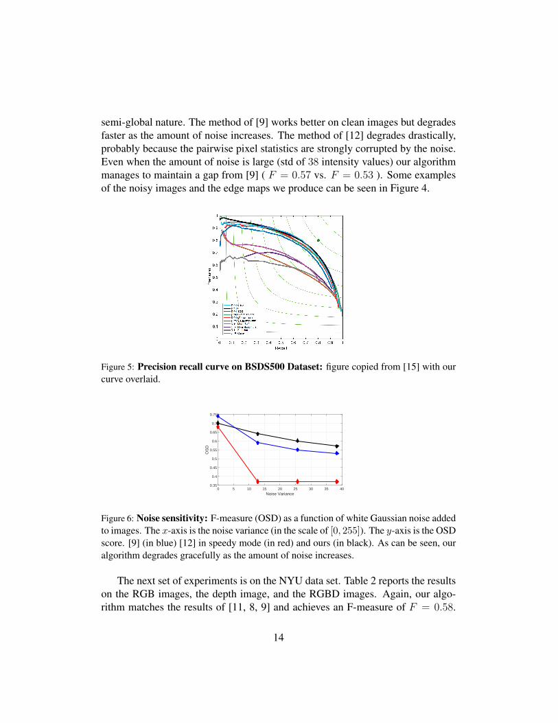
Figures 3 show results on the BSDS500 data set. In particular, we show theimages with the lowest/highest precision/recall. Figure 5 shows the ROC curve ofour method, along with several other methods.

Next we conduct an experiment to demonstrate the robustness of our algorithmto noise. In the experiment we add increasing amounts of noise to the BSDS500test images and compare our method to that of [9] and [12]. Results are reportedin Figure 6. As can be seen, our algorithm is quite robust to noise because of its

11

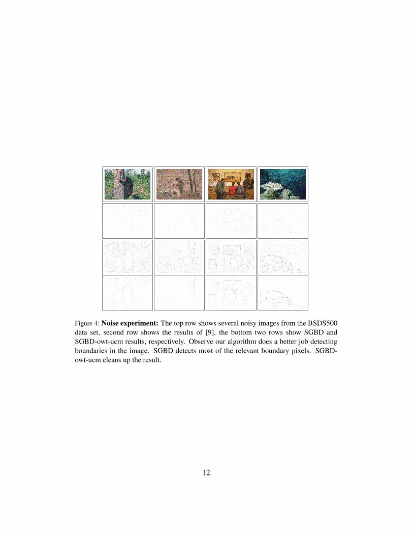
Figure 4: Noise experiment: The top row shows several noisy images from the BSDS500data set, second row shows the results of [9], the bottom two rows show SGBD andSGBD-owt-ucm results, respectively. Observe our algorithm does a better job detectingboundaries in the image. SGBD detects most of the relevant boundary pixels. SGBD-owt-ucm cleans up the result.

12

BSDS300Method OSD OIS APHuman 0.79 - -SCG[8] 0.71 - -gPb-owt-ucm[11] 0.71 0.74 0.73Gb[5] 0.67 - -BEL [6] 0.66 - -Canny [4] 0.58 0.62 0.58

SGBD-owt-ucm 0.69 0.71 0.69

BSDS500Method OSD OIS APHuman 0.80 0.80 -Crisp-MS, [12] 0.74 0.77 0.78SE-MS, T=4 [9] 0.74 0.76 0.78SCG [8] 0.74 0.76 0.77gPb-owt-ucm [11] 0.73 0.76 0.73Sketch Tokens [22] 0.73 0.75 0.78gPb[11] 0.71 0.74 0.65NCuts[23] 0.64 0.68 0.45MeanShift[24] 0.64 0.68 0.56Felz-Hutt[25] 0.61 0.64 0.56Canny[4] 0.60 0.63 0.58

SGBD-owt-ucm 0.72 0.74 0.72SGBD 0.70 0.72 0.73SGBD-naive 0.68 0.69 0.71

Table 1: Results on the BSDS dataset: Our results (bottom row) compared to recenttechniques.

13

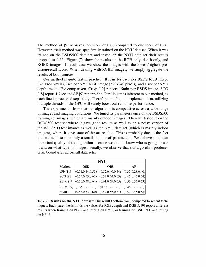
semi-global nature. The method of [9] works better on clean images but degradesfaster as the amount of noise increases. The method of [12] degrades drastically,probably because the pairwise pixel statistics are strongly corrupted by the noise.Even when the amount of noise is large (std of 38 intensity values) our algorithmmanages to maintain a gap from [9] ( F = 0.57 vs. F = 0.53 ). Some examplesof the noisy images and the edge maps we produce can be seen in Figure 4.

Figure 5: Precision recall curve on BSDS500 Dataset: figure copied from [15] with ourcurve overlaid.

Noise Variance0 5 10 15 20 25 30 35 40

OS

D

0.35

0.4

0.45

0.5

0.55

0.6

0.65

0.7

0.75

Figure 6: Noise sensitivity: F-measure (OSD) as a function of white Gaussian noise addedto images. The x-axis is the noise variance (in the scale of [0, 255]). The y-axis is the OSDscore. [9] (in blue) [12] in speedy mode (in red) and ours (in black). As can be seen, ouralgorithm degrades gracefully as the amount of noise increases.

The next set of experiments is on the NYU data set. Table 2 reports the resultson the RGB images, the depth image, and the RGBD images. Again, our algo-rithm matches the results of [11, 8, 9] and achieves an F-measure of F = 0.58.

14

(a) (b) (c) (d)

Figure 7: NYU Results top two rows RGB images, rows 3 and 4 depth images, rows 56 & 7 RGBD images. Columns show image with (a) min recall, (b) max recall, (c) minprecision, and (d) max precision.

15

The method of [9] achieves top score of 0.60 compared to our score of 0.58.However, their method was specifically trained on the NYU dataset. When it wastrained on the BSDS500 data set and tested on the NYU data set their resultsdropped to 0.55. Figure (7) show the results on the RGB only, depth only, andRGBD images. In each case we show the images with the lowest/highest pre-cision/recall score. When dealing with RGBD images, we simply aggregate theresults of both sources.

Our method is quite fast in practice. It runs for 8sec per BSDS RGB image(321x481pixels), 3sec per NYU RGB image (320x240 pixels), and 1 sec per NYUdepth image. For comparison, Crisp [12] reports 15min per BSDS image, SCG[18] report 1-2sec and SE [9] reports 6hz. Parallelism is inherent to our method, aseach line is processed separately. Therefore an efficient implementation, utilizingmultiple threads or the GPU will surely boost our run time performance.

The experiments show that our algorithm is competitive across a wide rangeof images and imaging conditions. We tuned its parameters once on the BSDS500training set images, which are mainly outdoor images. Then we tested it on theBSDS500 test set where it gave good results as well as on a noisy version ofthe BSDS500 test images as well as the NYU data set (which is mainly indoorimages), where it gave state-of-the-art results. This is probably due to the factthat we need to tune only a small number of parameters. We believe this is animportant quality of the algorithm because we do not know who is going to useit and on what type of images. Finally, we observe that our algorithm producescrisp boundaries across all data sets.

NYUMethod OSD OIS APgPb [11] (0.51,0.44,0.53) (0.52,0.46,0.54) (0.37,0.28,0.40)SCG [8] (0.55,0.53,0.62) (0.57,0.54,0.63) (0.46,0.45,0.54)SE-MS[9] (0.60,0.58,0.64) (0.61,0.59,0.65) (0.56,0.57,0.63)

SE-MS[9] (0.55, - , - ) (0.57, - , - ) (0.46, - , - )SGBD (0.58,0.53,0.60) (0.59,0.55,0.61) (0.52,0.45,0.58)

Table 2: Results on the NYU dataset: Our result (bottom row) compared to recent tech-niques. Each parenthesis holds the values for RGB, depth and RGBD. [9] report differentresults when training on NYU and testing on NYU, or training on BSDS500 and testingon NYU.

16

6. Conclusions

We presented a simple algorithm for boundary detection that relies on a SemiGlobal analysis of the image. The algorithm works on scan lines, which are a mid-level image representation, that is not purely local like patch based methods, yetis not global, as it does not work on the entire image. The reason for using scanlines is that they are 1D signals and as such we can use Dynamic Programming toefficiently find a globally optimal segmentation. This is based on the assumptionwe make that the boundaries between 1D segments are the boundary pixels in theimage. We gave a probabilistic analysis that suggests how to combine all the 1Dresults into a single coherent probabilistic 2D boundary map, and evaluated it on anumber of data sets. The algorithm is simple to implement, and works well acrossa wide range of data sets without any modification.

References

[1] H. Hirschmuller, Stereo processing by semiglobal matching and mutual in-formation, IEEE Trans. Pattern Anal. Mach. Intell. 30 (2) (2008) 328–341.

[2] D. Scharstein, R. Szeliski, A taxonomy and evaluation of dense two-framestereo correspondence algorithms, Int. J. Comput. Vision 47 (1-3) (2002) 7–42. doi:10.1023/A:1014573219977.URL http://dx.doi.org/10.1023/A:1014573219977

[3] A. Geiger, P. Lenz, R. Urtasun, Are we ready for autonomous driving? thekitti vision benchmark suite, in: Conference on Computer Vision and Pat-ternRecognition (CVPR), 2012.

[4] J. Canny, A computational approach to edge detection, Pattern Analysis andMachine Intelligence, IEEE Transactions on PAMI-8 (6) (1986) 679–698.doi:10.1109/TPAMI.1986.4767851.

[5] D. R. Martin, C. Fowlkes, J. Malik, Learning to detect natural image bound-aries using local brightness, color, and texture cues, IEEE Trans. PatternAnal. Mach. Intell. 26 (5) (2004) 530–549.

[6] P. Dollar, Z. Tu, S. Belongie, Supervised learning of edges and object bound-aries, in: CVPR (2), 2006, pp. 1964–1971.

17

[7] J. Mairal, M. Leordeanu, F. Bach, M. Hebert, J. Ponce, Discriminative sparseimage models for class-specific edge detection and image interpretation, in:ECCV (3), 2008, pp. 43–56.

[8] X. Ren, L. Bo, Discriminatively trained sparse code gradients for contourdetection, in: NIPS, 2012, pp. 593–601.

[9] P. Dollar, C. L. Zitnick, Structured forests for fast edge detection, in: ICCV,2013.

[10] M. Leordeanu, R. Sukthankar, C. Sminchisescu, Efficient closed-form solu-tion to generalized boundary detection, in: ECCV (4), 2012, pp. 516–529.

[11] P. Arbelaez, M. Maire, C. Fowlkes, J. Malik, Contour detection and hierar-chical image segmentation, IEEE Trans. Pattern Anal. Mach. Intell. 33 (5)(2011) 898–916.

[12] P. Isola, D. Zoran, D. Krishnan, E. H. Adelson, Crisp boundary detectionusing pointwise mutual information., in: ECCV (3), 2014, pp. 799–814.

[13] B. Andres, J. H. Kappes, T. Beier, U. Kothe, F. A. Hamprecht, Probabilisticimage segmentation with closedness constraints, in: ICCV, 2011, pp. 2611–2618.

[14] R. Bellman, On the approximation of curves by line segments using dynamicprogramming, Commun. ACM 4 (6) (1961) 284.

[15] R. Zabih, V. Kolmogorov, Spatially coherent clustering using graph cuts, in:CVPR (2), 2004, pp. 437–444.

[16] Y. Boykov, O. Veksler, R. Zabih, Fast approximate energy minimizationvia graph cuts, IEEE Trans. Pattern Anal. Mach. Intell. 23 (11) (2001)1222–1239. doi:10.1109/34.969114.URL http://doi.ieeecomputersociety.org/10.1109/34.969114

[17] Y. Boykov, M. Jolly, Interactive graph cuts for optimal boundary and regionsegmentation of objects in N-D images, in: ICCV, 2001, pp. 105–112.

[18] C. Rother, V. Kolmogorov, A. Blake, ”grabcut”: interactive foreground ex-traction using iterated graph cuts, ACM Trans. Graph. 23 (3) (2004) 309–314.

18

[19] X. Ren, J. Malik, Learning a classification model for segmentation, in: Proc.9th Int’l. Conf. Computer Vision, Vol. 1, 2003, pp. 10–17.

[20] R. Achanta, A. Shaji, K. Smith, A. Lucchi, P. Fua, S. Susstrunk,SLIC superpixels compared to state-of-the-art superpixel methods,IEEE Trans. Pattern Anal. Mach. Intell. 34 (11) (2012) 2274–2282.doi:10.1109/TPAMI.2012.120.URL http://dx.doi.org/10.1109/TPAMI.2012.120

[21] T. X. Han, S. Kay, T. S. Huang, Optimal segmentation of signals and itsapplication to image denoising and boundary feature extraction, in: ICIP,2004, pp. 2693–2696.

[22] J. J. Lim, C. L. Zitnick, P. Dollr, Sketch tokens: A learned mid-levelrepresentation for contour and object detection., in: CVPR, IEEE, 2013, pp.3158–3165.URL http://dblp.uni-trier.de/db/conf/cvpr/cvpr2013.html

[23] T. Cour, F. Benezit, J. Shi, Spectral segmentation with multiscale graph de-composition, in: 2005 IEEE Computer Society Conference on ComputerVision and Pattern Recognition (CVPR 2005), 20-26 June 2005, San Diego,CA, USA, 2005, pp. 1124–1131. doi:10.1109/CVPR.2005.332.URL http://dx.doi.org/10.1109/CVPR.2005.332

[24] D. Comaniciu, P. Meer, Mean shift: A robust approach toward feature spaceanalysis, IEEE Trans. Pattern Anal. Mach. Intell. 24 (5) (2002) 603–619.doi:10.1109/34.1000236.URL http://doi.ieeecomputersociety.org/10.1109/34.1000236

[25] P. F. Felzenszwalb, D. P. Huttenlocher, Efficient graph-based image seg-mentation, International Journal of Computer Vision 59 (2) (2004) 167–181.doi:10.1023/B:VISI.0000022288.19776.77.URL http://dx.doi.org/10.1023/B:VISI.0000022288.19776.77

19