semi-markov reliability model of the cold …jaqm.ro/issues/volume-5,issue-3/pdfs/grabski.pdf ·...

International Symposium on Stochastic Models

in Reliability Engineering, Life Sciences and Operations Management (SMRLO'10)

486

SEMI-MARKOV RELIABILITY MODEL

OF THE COLD STANDBY SYSTEM Franciszek GRABSKI Prof, Department of Mathematics and Physics, Polish Naval University, Gdynia, Poland E-mail: [email protected]

Abstract: The semi-Markov reliability model of the cold standby system with renewal is presented in the paper. The model is some modification of the model that was considered by Barlow & Proshan (1965), Brodi & Pogosian (1978). To describe the reliability evolution of the system, we construct a semi-Markov process by defining the states and the renewal kernel of that one. In our model the time to failure of the system is represented by a random variable that denotes the first passage time from the given state to the subset of states. Appropriate theorems from the semi-Markov processes theory allow us to calculate the reliability function and mean time to failure. As calculating an exact reliability function of the system by using Laplace transform is often complicated we apply a theorem which deals with perturbed semi-Markov processes to obtain an approximate reliability function of the system. Key words: semi-Markov process; perturbed process; reliability model; renewal standby system

1. Description and Assumptions

We assume that the system consists of one operating series subsystem (unit), an identical stand-by subsystem and a switch (see Figure 1):

1 2 N

N1 2

Figure 1. Diagram of the system



487

Each subsystem consists of N components. We assume that time to failure of those

elements are represented by non-negative mutually independent random variables kζ ,

Nk ,...,1= , with distributions given by probability density functions ( )xfk , 0≥x ,

Nk ,...,1= . When the operating subsystem fails, the spare is put in motion by the switch

immediately. The failed subsystem is renewed. There is a single repair facility. A renewal time is a random variable having distribution depending on a failed component. We suppose that the lengths of repair periods of units are represented by identical copies of non-negative

random variables kγ , Nk ,...,1= , which have cumulative distribution functions

( ) ( )xPxH kk ≤= γ , 0≥x . The failure of the system occurs when the operating subsystem

fails and the subsystem that has sooner failed in not still renewed or when the operating

subsystem fails and the switch also fails. Let U be a random variable having binary

distribution

where 0=U , if a switch is failed at the moment of the operating unit failure, and

1=U , if the switch works at that moment. We suppose that the whole failed system is

replaced by the new identical one. The replacing time is a non negative random variable η

with CDF

Moreover, we assume that all random variables mentioned above are independent.

2. Construction of Semi-Markov Reliability Model

To describe the reliability evolution of the system, we have to define the states and the renewal kernel. We introduce the following states:

0 – failure of the system;

k – renewal of the failed subsystem after a failure of k -th, Nk ,...,1= , component

and the work of a spare unit

1+N – both an operating unit and a spare are "up". The scheme shown in Figure 2 presents functioning of the system. Let

∗∗∗= 210 ,,0 τττ - denote the instants of the states changes, and ( ){ }0: ≥ttY be a random

process with the state space { }1,,...,1,0 += NNS , which keeps constant values on the half-

intervals [ ) ,...1,0,, 1∗+

∗nn ττ , and is right-hand continuous. This process is not a semi-Markov

one, as no memory property is satisfied for any instants of the state changes of that one.

Let us construct a new random process in a following way. Let 00 τ= and ,..., 21 ττ

denote instants of the subsystem failures or instants of the whole system renewal.

The random process ( ){ }0: ≥ttX defined by equation

(1)

is the semi-Markov one.



488

To have a semi-Markov process as a model we have to define its initial distribution and all elements of its kernel. Recall that the semi-Markov kernel is the matrix of transition probabilities of the Markov renewal process

(2)

I

II

ζ2

ζ1

ζΝ

ζ2

γ2

γ1

τ1 τ2 τ3τ4

t

γΝ

γΝ

τ∗1

τ∗2 τ∗

3 τ∗4 τ∗

5τ∗

6

0

Figure 2. Reliability evolution of the standby system

where

(3)

From the definition of semi-Markov process it follows that the sequence

( ){ },...1,0: =nX nτ is a homo-geneous Markov chain with transition probabilities

(4)

The function

(5)

is a cumulative probability distribution of a random variable iT that is called a

waiting time of the state i . The waiting time iT is the time spent in state i when the

successor state is unknown. The function

(6)

is a cumulative probability distribution of a random variable ijT that is called a

holding time of a state i , if the next state will be j . From here we have

(7)

It follows from that a semi-Markov process with a discrete state space can be

defined by the transition matrix of the embedded Markov chain: [ ]SjipP ij ∈= ,: and a

matrix of CDF of holding times: ( ) ( )[ ]SjitFtF ij ∈= ,: .

In this case semi-Markov kernel has a form



489

(8)

The semi-Markov ( ){ }0: ≥ttX will be defined if we define all elements of the

matrix .

For Nj ,...,1= we obtain

where

Using Fubini theorem we obtain

(9)

For 0=j we have

(10)

For Nji ,...,1, = we get

The same way we obtain

(11)

For Ni ,...,1= and 0=j we have

(12)

where

(13)

From the assumption it follows that (14)



490

All elements of the kernel have been defined, hence the semi-Markov process

( ){ }0: ≥ttX describing reliability of the renewal cold standby system has been constructed.

3. Exponential Time to Failure of Elements

Assuming the exponential time to failure of elements we obtain a special case of

the model. Suppose that random variables kζ , Nk ,...,1= are exponentially distributed

with parameters kλ , Nk ,...,1= , correspondingly. Hence

Because of the no memory property of the exponential distribution, the assumption

concerning of the whole subsystem renewal can be substituted by the assumption concerning failed element renewal.

In this case we obtain

(15)

for Nj ,...,1= , where

For 0=j we obtain

(16)

For Nji ,...,1, =

(17)

For 0=j

(18)

4. Approximate Model

For simplicity we consider an approximate model. We can assume that the renewal time of the subsystem is a random variable γ having CDF

(19)

This way we obtain 3-state semi-Markov process with kernel

, (20)

where (21)



491

(22)

Assume that, the initial state is 2 . It means that an initial distribution is

(23)

Hence, the semi-Markov model has been constructed.

5. Reliability Characteristics

A value of a random variable

(24)

denotes a discrete time (a number of state changes) of a first arrival at the set of

states SA ⊂ of the embedded Markov chain .

(25)

denotes a first passage time to the subset A or the time of a first arrival at the set

of states SA ⊂ of the semi-Markov process ( ){ }0: ≥ttX . A function

(26)

is the Cumulative Distribution Function (CDF) of a random variable denoting

the first passage time from the state to a subset A or the exit time of ( ){ }0: ≥ttX

from the subset with the initial state . We will present some theorems concerning

distributions and parameters of the random variables which are conclusions from theorems presented by Koroluk & Turbin (1976), Silvestrov (1980), Grabski (2002).

THEOREM 1 For the regular semi-Markov processes such that,

(27)

distributions are proper and they are the unique solutions of the

equations system

. (28)

Applying a Laplace-Stieltjes (L-S) transformation for the system of integral equations we obtain the linear system of equations for (L-S) transforms

(29)

where

(30)

are L-S transforms of the unknown CDF of the random variables , and

(31)



492

are L-S transforms of the given functions . That linear system of

equations is equivalent to the matrix equation

, (32)

where (33)

is the unit matrix, (34)

is the square sub-matrix of the L-S transforms of the matrix while

(35)

are one column matrices of the corresponding L-S transforms. The linear system of equations (29) for the L-S transforms allows us to obtain the

linear system of equations for the moments of random variables

THEOREM 2 If • assumptions of theorem 1 are satisfied, •

•

then there exist expectations and second moments

and they are unique solutions of the linear systems equations, which have

following matrix forms

(36)

where

(37)

where

,

and is the unit matrix.

In our case the random variable , that denotes the first passage time from the state to the subset represents the time to failure of the system in our model.

The function (38)

is the reliability function of the considered cold standby system with repair. In this case the system of linear equations (29) for the Laplace-Stieltjes transforms

with the unknown functions is

(39)

Hence



493

(40)

Consequently, we obtain the Laplace transform of the reliability function

(41)

The transition matrix of the embedded Markov chain of the semi-Markov process

( ){ }0: ≥ttX is

, (42)

where

The of the waiting times are

Hence

(43)

In this case equation (37) takes the form of

(44)

The solution of it is:

(45)

6. An Approximate Reliability Function

In this case calculating an exact reliability function of the system by means of Laplace transform is a complicated matter. Finding an approximate reliability function of that system is possible by using results from the theory of semi-Markov processes perturbations. The perturbed semi-Markov processes are defined in different ways by different authors. We introduce Pavlov and Ushakov (1978) concept of the perturbed semi-Markov process presented by I.B. Gertsbakh (1984).

Let be a finite subset of states and be at least countable subset of

. Suppose ( ){ }0: ≥ttX is SM process with the state space and the kernel

, the elements of which have the form .

Assume that

(46)

and

(47)



494

Let us notice that .

A semi-Markov process ( ){ }0: ≥ttX with the discrete state space defined by the

renewal kernel , is called the perturbed process with respect to

SM process with the state space defined by the kernel

.

We are going to present our version of theorem proved by I.B. Gertsbakh (1984). The number

(48)

where

(49)

is the expected value of the waiting time in state for the process .

Denote the stationary distribution of the embedded Markov chain in SM process

by . Let

(50)

We are interested in the limiting distribution of the random variable , that denotes the first passage time from

the state to the subset .

THEOREM 3 If the embedded Markov chain defined by the matrix of transition probabilities

satisfies the following conditions

(51)

(52)

(53)

then

(54)

where is the unique solution of the linear system of equations

(55)

From that theorem it follows that for small we get the following approximating formula

(56)



495

The considered SM process with the state space we

can assume to be the perturbed process with respect to the SM process

with the state space and the kernel

(57)

where

(57)

Because and

(57)

then

(57)

From

(57)

we get

(57)

Notice, that . Hence . Finally we obtain

(57)

The transition matrix of the embedded Markov chain of SM process

is

(58)

From the system of equations

(59)

we get . It follows from the theorem 3 that for a small

(60)

where

(61)

and



496

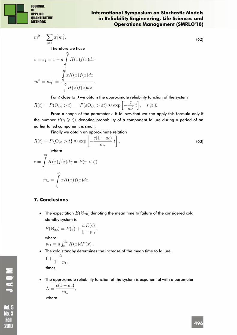
(62)

Therefore we have

(62)

For close to we obtain the approximate reliability function of the system

(62)

From a shape of the parameter it follows that we can apply this formula only if

the number , denoting probability of a component failure during a period of an

earlier failed component, is small. Finally we obtain an approximate relation

(63)

where

(62)

7. Conclusions

• The expectation denoting the mean time to failure of the considered cold

standby system is

where

.

• The cold standby determines the increase of the mean time to failure

times.

• The approximate reliability function of the system is exponential with a parameter

where



497

References

1. Barlow, R.E. and Proshan, F. Mathematical Theory of Reliability, Wiley: New-York, London,

Sydney, 1965 2. Brodi, S.M. and Pogosian, I.A. Embedded Stochastic Processes in the Queue Theory, Naukova

Dumka, Kiev, 1978 (in Russian) 3. Gertsbakh, I.B. Asymptotic methods in reliability theory: A review, Adv. Appl. Prob., 16, 1984,

pp. 147-175 4. Grabski, F.G. Semi-Markov model of reliability and operation, PAN IBS, Operation Research,

30, Warszawa, 2002, pp. 161 (in Polish) 5. Grabski, F.G. Applications of Semi-Markov processes in safety and reliability analysis,

SSARS 2009, Gdańsk, 2009, pp. 94 6. Koroluk, W.S. and Turbin, A.F. Semi-Markov Processes and Their Applications, Naukova

Dumka, Kiev, 1976 (in Russian) 7. Pavlov, I.V. and Ushakov, I.A. The asymptotic distribution of the time until a semi-Markov

process gets out of the kernel, Engineering Cybernetics, 20 (3), 1978 8. Silvestrov, D.S. Semi-Markov Processes with Discrete State Space, Sovietskoe Radio, Moscow,

1980 (in Russian)

semi-markov reliability model of the cold …jaqm.ro/issues/volume-5,issue-3/pdfs/grabski.pdf ·...

Documents