POLITECNICO DI TORINO

Master’s Degree in Communication and Computer NetworksEngineering

Master’s Thesis

Semi-persistent data schedulinganalysis over ultra low latency

communication networks

AdvisorCarla Fabiana ChiasseriniCo-advisor:Jérôme Härri

Candidate

Alberto LamorteID number 252880

Academic Year 2019-2020

Abstract

In this thesis we analyse performances of communication in a railway environment,where requirements are very strict in terms of latency and reliability. Nowadayson the train backbone, time sensitive networks are used because they meet thosestrict requirements.

The scope of this thesis is to analyse performances of different algorithms to seeif it is possible with current technologies to provide a wireless connection above thetime sensitive network, working on the so called wireless train backbone, and prac-tically implement a wireless link in a wired network. The first scheduling algorithmthat are analysed is the semi-persistent scheduling, the algorithm currently stan-dardized by 3GPP for cellular communications without the eNodeB coordination.The algorithm is tested using NS3, a network simulator. The second algorithmthat is tested is the self-organized time division multiple access algorithm. This al-gorithm has been tested in vehicular environment and under certain condition hasshown better performances then semi-persistent scheduling algorithm. In this the-sis it is tested using a MATLAB implementation and applied on the same scenarioof semi-persistent scheduler.

Dans cette thèse, nous analysons les performances de communication dans unenvironnement ferroviaire, où les exigences sont très strictes en termes de latenceet de fiabilité. De nos jours sur la dorsale du train, des réseaux sensibles au tempssont utilisés car ils répondent à ces exigences strictes.

Le but de cette thèse est d’analyser les performances de différents algorithmespour voir s’il est possible avec les technologies actuelles de fournir une connexionsans fil au-dessus du réseau sensible au temps, en travaillant sur ce que l’on appellela dorsale du train sans fil, et de mettre en œuvre pratiquement une liaison sans fildans un réseau câblé. réseau. Le premier algorithme d’ordonnancement analysé estl’ordonnancement semi-persistant, l’algorithme actuellement standardisé par 3GPPpour les communications cellulaires sans la coordination eNodeB. L’algorithme esttesté à l’aide de NS3, un simulateur de réseau. Le deuxième algorithme testé estl’algorithme d’accès multiple à répartition dans le temps auto-organisé. Cet algo-rithme a été testé en environnement véhiculaire et dans certaines conditions a mon-tré de meilleures performances que l’algorithme de programmation semi-persistant.Dans cette thèse, il est testé à l’aide d’une implémentation MATLAB et appliquésur le même scénario de planificateur semi-persistant.

ii

Acknowledgements

I would like to thank my supervisor Jérôme Härri for all the suggestions, thepatience and all the time he dedicated me. I would thank my supervisor CarlaChiasserini for the support she gave me, as well as the hope when difficult periodcame.

would say thank you to my family for love I receive from them, the courage Ineeded and because they spurred me to be more determined.

I want to thank all my friends for all the time they dedicated me, for all theenergy I needed.

i

Contents

List of Tables iii

List of Figures iv

1 Introduction 1

2 State of the art 42.1 TSN: application for ultra reliable and low latency communications 42.2 Wireless TSN . . . . . . . . . . . . . . . . . . . . . . . . . . . . . . 62.3 3GPP C-V2X roadmap . . . . . . . . . . . . . . . . . . . . . . . . . 7

2.3.1 Release 12 and 13 . . . . . . . . . . . . . . . . . . . . . . . . 92.3.2 Release 14 and 15 . . . . . . . . . . . . . . . . . . . . . . . . 122.3.3 Release 16 . . . . . . . . . . . . . . . . . . . . . . . . . . . . 15

2.4 C-V2X schedulers . . . . . . . . . . . . . . . . . . . . . . . . . . . . 172.4.1 Semi-Persistent Scheduling (SPS) . . . . . . . . . . . . . . . 172.4.2 Self-organized Time Division Multiple Access (STDMA) . . 202.4.3 OOC codes . . . . . . . . . . . . . . . . . . . . . . . . . . . 25

3 Analytical study and simulations 273.1 Perfect scheduler analysis . . . . . . . . . . . . . . . . . . . . . . . 273.2 Network Simulator and workflow . . . . . . . . . . . . . . . . . . . 303.3 Simulations . . . . . . . . . . . . . . . . . . . . . . . . . . . . . . . 31

3.3.1 Simulations using semi-persistent scheduler . . . . . . . . . . 313.3.2 Simulations using optical orthogonal codes . . . . . . . . . . 353.3.3 Comparison between semi-persistent scheduler and optical

orthogonal codes scheduler . . . . . . . . . . . . . . . . . . . 42

4 Conclusion and future work 444.1 Conclusion . . . . . . . . . . . . . . . . . . . . . . . . . . . . . . . . 444.2 Future works . . . . . . . . . . . . . . . . . . . . . . . . . . . . . . 45

Bibliography 46

ii

List of Tables

2.1 5G V2X services requirements . . . . . . . . . . . . . . . . . . . . . 142.2 Multiple numerologies in NR . . . . . . . . . . . . . . . . . . . . . . 152.3 SPS RRI parameter . . . . . . . . . . . . . . . . . . . . . . . . . . . 182.4 STDMA system parameters description . . . . . . . . . . . . . . . . 22

3.1 Perfect scheduler . . . . . . . . . . . . . . . . . . . . . . . . . . . . 293.2 Conversion from density and inter-antenna distance . . . . . . . . . 333.3 2D-1D table conversion . . . . . . . . . . . . . . . . . . . . . . . . . 39

iii

List of Figures

2.1 Sidelink possible scenarios . . . . . . . . . . . . . . . . . . . . . . . 82.2 ProSe reference architecture extension . . . . . . . . . . . . . . . . 92.3 Structure of Sidelink resource pool . . . . . . . . . . . . . . . . . . 102.4 Example of sidelink time/frequency allocation . . . . . . . . . . . . 112.5 Reference signals disposition . . . . . . . . . . . . . . . . . . . . . . 122.6 PHY description . . . . . . . . . . . . . . . . . . . . . . . . . . . . 132.7 NR PHY description . . . . . . . . . . . . . . . . . . . . . . . . . . 162.8 STDMA parameters . . . . . . . . . . . . . . . . . . . . . . . . . . 232.9 OSTDMA representation . . . . . . . . . . . . . . . . . . . . . . . . 242.10 Distributed allocation: OOC-based access to slots . . . . . . . . . . 26

3.1 Scenario representation . . . . . . . . . . . . . . . . . . . . . . . . . 283.2 Workflow representation . . . . . . . . . . . . . . . . . . . . . . . . 313.3 Comparison between STDMA and OOC . . . . . . . . . . . . . . . 323.4 PRR over distance with SPS . . . . . . . . . . . . . . . . . . . . . . 333.5 PRR over density for different TX-RX distance with SPS . . . . . . 343.6 PRR survival function with SPS . . . . . . . . . . . . . . . . . . . . 353.7 PRR for different packet size with SPS . . . . . . . . . . . . . . . . 363.8 PRR over variable packet size with SPS scheduler . . . . . . . . . . 373.9 Scenario representation . . . . . . . . . . . . . . . . . . . . . . . . . 373.10 PRR over density with OOC . . . . . . . . . . . . . . . . . . . . . . 383.11 PRR over distance with OOC . . . . . . . . . . . . . . . . . . . . . 393.12 PRR survival function with OOC scheduler . . . . . . . . . . . . . . 403.13 PRR over different packet size with OOC scheduler . . . . . . . . . 413.14 PRR over variable packet size with OOC scheduler . . . . . . . . . 423.15 PRR over different modulation with OOC scheduler . . . . . . . . . 43

iv

Chapter 1

Introduction

Vehicular communications are getting more and more important in communi-cation field, because it is thought that autonomous driving would provide bettersafety, as stated in [1], and efficiency, in respect with human driven mobility, moreprone to errors. In [2] they estimate that autonomous driving would decrease traffic,it would reduce carbon oxide emission, increasing mobility. Car-to-car and car-to-infrastructure communication are just few examples of communications needed forthis technological transition, but the evolution of mobility is not just related to cardriving.

Inspired by car environment, the same idea could be extended in the railwayenvironment, thinking in the future about autonomous-driven trains. Nowadaysthe trains are spaced in the system in inefficient way, because the space amongone train and the following one must be very high for safety reason, exploitingpoorly the infrastructure capacity. Moreover, the train structure itself is rigidand this rigidity implies many disadvantages in terms of maintenance and trafficengineering. Using the same idea of car environment, the consists in a train can beseen as independent and a track can evolve ongoing by single consists that can joinor leave the group, according to their destination. A similar concept is used in carmobility by platooning, where cars, or trucks, could create groups of vehicle rollingcompact, in order to save space and reduce air friction. In order to establish thiskind of groups of vehicle, all the members must be in communication. This kind ofcommunications are challenging in terms of reliability and latency.

In the trail-way environment, the requirements are strict because high speed isinvolved, and high density can be a possible scenario trains mast be able to manage.The industrial requirements for latency must stay below 1 ms and for reliability of1 packet lost every 106, and they are similar to railway communication in order todeal with high speed and low distance among consists. This kind of requirementsare met in industrial environment by time sensitive networks (TSN). This kindof wired networks have all synchronized nodes and evident latency restriction pernode in the network, as well as high reliability and limited jitter.

1

Introduction

Currently all the consists in a train are physically linked and so wired. ONone hand this connection is effective for low interference and implementation ofTSN, but, on the other hand, this network is static. Physically separation amongconsists in the train means exploit a wireless channel among consists for controland management communication, forming the so called Wireless train backbonecommunication (WLTB), as stated in one of objectives in [3]. Exploiting a wirelessconfiguration, the advantage resides in the flexibility and scalability of the com-munication inside the train. Moreover, the train topology can be variable so thatspace efficiency can improve.

So the main scope of the project is to find a way to introduce wireless links insidea local area network that satisfies time sensitive networks standard and continue tosatisfy the standard independently from wireless or wire links: wireless links shouldnot impact on the time sensitiveness of the network.

For wireless communication there are different possibilities. First of all a wifiapproach was discussed, in particular the newest IEEE 802.11 BD, for the technol-ogy capability to naturally handle local area networks. As major alternative, 5Gapproach was considered for the capabilities of this technology. These two tech-nologies are deeply explained and analysed in [4]. It is important to mention thatfrom long time there is a comparison among cellular technology and wifi technology,discussing which one is better for vehicle communication. Thinking at the data rateconstrains, visible light communication was considered. This technology, describedin [5], is already proposed for vehicle platooning as analysed in [6]. Lastly, concern-ing the cellular communication, the 4G approach was considered because of someadvantages such as already existing protocols and prototypes. In particular the C-V2X already standardized by 3GPP offer two possibilities: LTE D2D, standardizedin releases 12 and 13, and LTE V2X, standardized in releases 14 and 15.

Safe4RAIL analysed all the proposals already described and finally decided tochoose the LTE V2X approach for market availability, because a ready prototypewas important to speed up the process of real implementation. Among the issuesthis kind of approach has, the main question is how good the standardized scheduler,the so called semi-persistent scheduler, or in other words, the main question is ifthe standardized scheduler can satisfy latency requirements and how reliable it is.

In chapter 2 we would study some literature about resource allocation andscheduling, vehicular networks and proximity service. In particular we would ex-plain the static and dynamic allocation, the exploitation of vehicle computing ca-pabilities for a cloud-based scheduling and finding optimal solutions using gametheory

A study would be performed in section 3.3 to determinate if this algorithm isstrong enough. For this purpose, we will study the algorithm response in functionof packet size, inter-distance among vehicles, variable packet size and a study aboutreliability. An alternative on this algorithm is present in Optical Orthogonal Codes(OOC), a scheduler that is considered a valid alternative to Dedicated Short range

2

Introduction

communication DSRC standard. This second scheduler would be simulated inMATLAB algorithm in section 3.3 and would be compared with the results obtainby NS3 simulation of semi-persistent scheduler.

Finally in chapter 4 we report our comments and conclusions and we explain allthe future works can be developed starting from this thesis.

3

Chapter 2

State of the art

In this chapter we illustrate the most recent studies about resource allocation,scheduling in vehicular environment in general.

We then analyse more deeply the structure of semi-persistent scheduling and self-organizing time division multple access, in order to have a clearer idea about howthey work and how they would be used in the simulations performed in section 3.3.

2.1 TSN: application for ultra reliable and low la-tency communications

Latency, as it is defined in [7], is the time elapsing from the instant of thebeginning of transmission by the transmitter to the complete reception by receiver.The term ultra-low-latency (ULL) refers to latencies in the order of few millisecondsor less then one millisecond.

ULL applications often require the so called deterministic latency or in otherwords, the latency must not exceed a certain bound, an example of application ofthis kind is industrial automation. Some others may require the so called proba-bilistic latency, i.e. a pre-determined delay bound that are met with a pre-definedprobability; an example of these applications is a multimedia streaming. In orderto guarantee these strict requirements the time sensitive networks are used.

TSN is standardized by IEEE 802.1 working group. Its aim is to develop stan-dards in areas like LAN/MAN architectures, inter-networking among IEEE 802LANs and MANs, security, IEEE 802 network management, protocol layers higherthan MAC and LLC layer. Their work is continuously revised: the current stan-dard is IEEE 802.1Q-2018. The standard specifies the bridge as a network entitywithin 802.1 enable communication among TSN network and an external networklike a IEEE 802 LAN. It is important to notice that TSN can be deployed over Eth-ernet, to support real-time industrial automation and control system applications.In case instead the physical layer used in the bridge is wireless, then some PKI are

4

State of the art

normally used, depending on applications.

[8] illustrates that the initial standardization had started with IEEE 802.1 Audioand Video Bridging, but then the task group evolved into time sensitive network-ing task group in 2012 because other user cases like industrial and automotiveapplication were taking into account.

The most useful standards for the scope of this thesis are the IEEE 802.1AS-2011and IEEE 802.1Q-2018. The former standard describes timing and synchronizationfor time-sensitive application in bridged local area networks, while the latter stan-dard deals in general with bridges and bridged networks. In particular inside IEEE802.1Q-2018 the amendment IEEE 802.1Qbv describes the scheduled traffic.

The standard specifies the flow concept, characterized by quality of service re-quirements like latency or bandwidth requirements. The definition of TSN flow asstated in [7] is "an end-to-end unicast or multicast network connection from oneend station (talker, sender) to another station(s) (listener(s), receiver(s)) thoughtthe time-sensitive capable network"; the term flow is sometimes referred as stream.Each TSN flow is defined by a priority code and by VLAN ID. In order to guaran-tee requested resources, the network has admission control and stream reservationprocedures. These procedures are performed in a centralized or distributed man-ner, depending on the complexity of the network, using the recommended YANGmodel and NETCONF protocol to configure network devices. Lastly, Path controlelement protocol uses existing routing algorithm for traffic-engineered networks.

Is important that each node is synchronized with the others, so that the networkbecame time-aware and can compute peer path delay and residence time inside eachnode: these information are fundamental for the scheduler and for routing choices.All the nodes’clock synchronization process is based on master-slave hierarchy andit is described in the standard IEEE 802.1AS-REV.

The concept of delay in TSN networks, do not care about average delay norfastest delivery, but the most important parameter is the worst case delay. Inorder to reduce the delay as small as possible each node has some traffic shapingpolicies. Moreover, to deal better with scheduled traffic slots, during which somepackets of certain TSN flow are forwarded by a node, a guard band is introduced,whose size is the largest possible interfering fragment. In this way the node can usepreemption and manage more effectively the traffic.

Due to very high reliability requirements, some mechanisms of packets repli-cation is used. They are replicated taking care of address, traffic class and pathinformation. Nodes must have duplicate frame elimination capability, in order torecognise packet replica and eventually drop them. The management of packetreplication is not trivial and to implement this function a centralized managementis required.

5

State of the art

2.2 Wireless TSN

In Release 16, 3GPP has considered the possibility to integrate time sensitivenetworking networks into 5G systems. As stated in [9], 3GPP has supported TSNconfiguration models, internetworking with TSN, simplified traffic scheduling, timesyncronization features and time sensitive communication traffic classes. Practi-cally, in release 16, a 5G network node can be seen as a logical TSN bridge and theentire network as a TSN network.

In [9] is mention anywhere the possibility of a wireless 5G connection that satis-fies TSN requirements. Wireless links are more prone to errors and delays, due tointerference; also security could be an issue.

In the following we would illustrates some studies to have a wireless link thatsatisfies TSN characteristics. In order to do so, the most important feature todefine are requirements. For different applications, we have different requirementsto satisfy. For example, in [10] the machine type communication has constrains onreliability at 99.999% and on latency set to 1 ms. For [11], in industrial environment(motion-control), the maximum end to end latency cannot exceed 0.1 ms and thereliability must be 99.9999%. As [12], Intelligent transportation system must satisfythe same requirements of URLLC so again e2e latency of 1 ms and reliability of99.999%. For what concern the Safe4RAIL requirements, listed in [] the maximumallowed end-to-end latency must be lower than cycle time of 40 ms and a reliabilityof 99,999%, or in other words, a probability of error equal to 0,001 percent, it meansone error every hundred thousand transmissions.

In order to define the key challenges towards wireless TSN networks, the AvnuAlliance wrote a white paper published in January 2018. The Avnu Alliance isa consortium consisting of professional, automotive, consumer electronics and in-dustrial manufacturing companies, working on defining a common certification foriter-operable TSN standards. In the white paper written by Steven F. Bush etal. [13], they state five points to meet in order to deploy wireless TSN: wirelessconfiguration of wired TSN, hybrid wired-wireless time synchronization, wirelessTSN scheduling, wireless redundancy for wired TSN and wireless TSN switch de-ployment.

The paper states that wireless configuration and switch deployment are rela-tively easy, the other phases have some gaps: tightness of synchronization, thepossibility of a wireless scheduler to be compliant with IEEE 802.2Qv, that wouldbe configurable and take care of synchronization errors, the integrability of wirelessinterface into IEEE 802.1CB seamlessly.

Furthermore, the paper raises an issues related to cybersecurity. Indeed, au-thentication and availability are the most important functions into an industrialsystem. In order to get them, the paper suggests the use of private key exchangeand for transmitting he keys, they encourage to take care of the development ofquantum key distribution and they suggest the use of IEEE P1913 keychain YANG

6

State of the art

model to manage key lifetimes.Finally, [13] concludes arguing that the most challenging issue is reliability with

determinism, because even if latency requirements can be met and retransmissioncan be considered to improve reliability, the target message must reach its destina-tion before the end of the scheduled period, to satisfy deterministic property.

The paper written by A. Mildner et al. in May 2019 [14] first considers the fourkey pillars: time synchronization, bounded low latency, ultra reliability and resourcemanagement. Considering as wireless medium a IEEE 802.11 physical layer, theauthors have focused on the IEEE 1588v2 Precision Time Protocol (PTP), and802.11 Beacon Frames and the internal Time Synchronization Function (TSF) forsynchronizing clocks. For what concern ultra reliability and low latency, they saythat even if we could consider retransmission into the latency period, the concept oflatency and determinism is still under research. Finally, the resource management ispossible exploiting wireless channel and it is more flexible than wired network. Thefinal conclusions of the paper states that the wireless deployment of time sensitivenetworking is still at early development stage, especially for what concern clocksynchronization and resource scheduling to meet bounded latency.

We can conclude after having analysed the current state of the art regardingwireless deployment of time sensitive networking that the implementation is still atinitial stage and many gaps must be filled. One of the most important issues stillremain the use of a scheduler capable of guaranteeing a bounded latency. So in thefollowing we explore some known scheduler and their performances.

2.3 3GPP C-V2X roadmap

In order to implement the communication among consists we need to chooseamong different technologies. As reported in [15], Safe4RAIL has considered LTE,ZigBee, WirelessHART, Ultra Wide Band, Wi-Fi, ECHORING, Wireless Interfacefor Sensors Actuators, as well as futures technologies like SHARP, LTE Release 15and 16 (5G), WirelessHP and Wifi 6 (IEEE 802.ax). Taking care of advantagesand disadvantages from every technology the Safe4Rail2 consortium has chosenthe LTE V2X technology as most appropriate for the scope of the project. In thefollowing we would describe how C-V2X communication has evolved release afterrelease, and how the 5G would modify it.

Since 3GPP release 12, a new interface was introduced: the so called PC5 overwhich the sidelink relies on. The sidelink is a new idea that add new functionalityto the communication: users can communicate directly without necessarily rely ona base station. The sidelink is neither an uplink channel nand a downlink channel,but it is defined as a third independent channel. For its configuration, the sidelink ismore similar to uplink than the downlink, because relies on the same single carrierfrequency division multiple access (SC-FDMA) used in LTE uplink.

7

State of the art

The main use of the sidelink is when the users are out of cell coverage: in thisscenario they must communicate without the presence of a base station. This sce-nario implies a completely distributed management of resources. A second possiblescenario is when just one user is in coverage but the other one is not covered bythe base station. In this second scenario the first user can receive some informationfrom the base station and handle the sidelink communication, reducing to the mini-mum the interference with the eventual users inside the cell. The second user wouldfollow the first user choices because it would know the first one is under coverage.A third possible scenario is when both users are in coverage of a base band. Inthis configuration they can decide if communicate through the base station as innormal cellular communication, or they could exploit the sidelink to communicatedevice to device. The advantage of this scenario in respect with the first one is thatthe base station have all scheduling information of users inside the cell and cansuggest a proper resource scheduling to D2D users, in order to reduce interferenceas much as possible. It must be noticed that uplink and downlink communicationhave higher priority than D2D communication, so in case the cell has reached themaximum capacity, the D2D communication cannot be a feasible choice.

Figure 2.1. Sidelink possible scenarios

The sidelink can be different, depending on modes. From rel. 12 to rel. 15, upto 4 modes have been defined: mode 1 and mode 2 are defined in rel. 12, theyare enhanced in rel. 13, mode 3 and mode 4 are defined in rel. 14. In rel. 15,3GPP has enhanced the 4 modes with some extra services. Finally, in rel. 16, thatwill be frozen in March 2020, they will introduce an optional second interface withimproved performances, known as NR V2X, consisting on 2 different modes andeventually 4 sub-modes for mode 2. Looking into the future development, release17, scheduled for delivery in 2021, has the following objectives: NR Sidelink en-hancement, NR Sidelink relay, Proximity based services in 5GS and enhancementsof V2X services.

8

State of the art

2.3.1 Release 12 and 13

Starting from Release 12 of LTE standard, 3GPP has formalized the Device-to-Device communications under the name of Proximity Services (ProSe). ProSeintroduce an extension to the classic LTE reference architecture, defining new net-work elements, new functions and new set of interfaces as illustrated in Figure 2.2

Figure 2.2. ProSe reference architecture extension (from [16]), section 4.2

Alongside the classical interfaces Uu (which connects the UEs with the eNodeB),numerous new interfaces (PC1 to PC8 and SGi) enable direct communicationsbetween devices without requiring the data flow to pass through the network. ThePC5 interface represents the air interface between UEs: it is denominated Sidelink,to distinguish it from the classic Uplink and Downlink that take place on the Uuinterface.

Sidelink communications are based on the concept of resource pools, which de-termine the subsets of the UL resources that are dedicated to a specific UE-to-UEchannel. Resource pools are formed by:

• subframe pool (in time domain), identifying a subset of the subframes

• resource block pool (in frequency domain), a subset of the PRBs

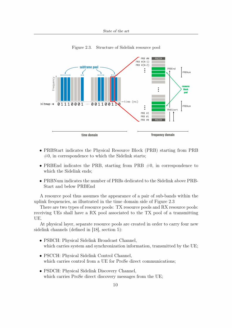
as illustrated in Figure 2.3.In the time domain, the subframe pools are laid out according to a periodic

structure. The channel occupation within the periods is determined by bitmaps(such as, for instance, the subframeBitmap-r12 in [17], section 6.3.8), whose ‘1’ bitsdenote the subframes which are part of the resource pool, as illustrated in the timedomain side of Figure 2.3.

Within each subframe marked with a ’1’, a resource block pool is defined infrequency domain by three parameters:

9

State of the art

Figure 2.3. Structure of Sidelink resource pool

• PRBStart indicates the Physical Resource Block (PRB) starting from PRB#0, in correspondence to which the Sidelink starts;

• PRBEnd indicates the PRB, starting from PRB #0, in correspondence towhich the Sidelink ends;

• PRBNum indicates the number of PRBs dedicated to the Sidelink above PRB-Start and below PRBEnd

A resource pool thus assumes the appearance of a pair of sub-bands within theuplink frequencies, as illustrated in the time domain side of Figure 2.3

There are two types of resource pools: TX resource pools and RX resource pools:receiving UEs shall have a RX pool associated to the TX pool of a transmittingUE.

At physical layer, separate resource pools are created in order to carry four newsidelink channels (defined in [18], section 5):

• PSBCH: Physical Sidelink Broadcast Channel,which carries system and synchronization information, transmitted by the UE;

• PSCCH: Physical Sidelink Control Channel,which carries control from a UE for ProSe direct communications;

• PSDCH: Physical Sidelink Discovery Channel,which carries ProSe direct discovery messages from the UE;

10

State of the art

• PSSCH: Physical Sidelink Shared Channel,which carries data from a UE for ProSe Direct Communication.

ProSe supports both one-to-one and one-to-many communication paradigms,although the latter is reserved to public safety UEs, as expressed in [16]

ProSe supports two communications modes, which differ on the allocation schemeadopted for transmission of the Sidelink Control Information (SCI) on the sidelinkcontrol channel (PSCCH):

• Mode 1: scheduled resource allocation

• Mode 2: autonomous resource selection

In mode 1, transmissions on the Sidelink are authorized by the installed net-work, which provides the transmitting UE with PSCCH resources to transmit theSCI in, and PSSCH resources to transmit data in. In mode 2, transmissions areunsupervised: transmitting UEs randomly choose the resources, within the PSCCHresource pool, in which to transmit the SCI.

The four sidelink physical channels are periodically interleaved in time, withperiodicity equal to one Sidelink Control Period as illustrated in Figure 2.4, anexample related to communication mode 2, wherein a PSSCH pool is staticallyallocated.

Figure 2.4. Example of sidelink time/frequency allocation

All the channels are implemented using OFDMA. The multiple access by dif-ferent users is achieved by assign different sub-carrier frequencies. The available

11

State of the art

bandwidth is composed by resource blocks in frequency domain. Every resourceblock is composed by 12 sub-carriers each 15kHz wide. In time domain instead, aframe last for 10 ms, and it is divided into subframes, 1 ms long. Each subframe isfurther divided into two slots whose length is 0.5 ms. The resource block, in time,last for one slot in the time domain.

2.3.2 Release 14 and 15

In 3GPP release 14, short-range LTE V2X was defined, thus they introducedmode 3 and mode 4 in addition to the previous mode 1 and mode 2 from D2Dcommunication. A new D2D interface is thus designed specifically for V2V com-munication, so specifically addressed for high speed nodes (maximum consideredspeed at 250 km/h [19]) and high density network (up to thousands of nodes).

To cope with high speed - and thus with Doppler effect - additional demodulationreference signal symbols are added to the channel, according to Figure 2.5.

Figure 2.5. Reference signals disposition, from [20]

Secondly, to reduce latency and satisfy V2V requirements, in mode 3 and 4the resource structure is changed in respect with mode 1 and 2. In particularthe PSCCH contain the sidelink control information (SCI) also called schedulingassignment (SA), that is used by the receiver to know the organization of the radioresources in PSSCH. The SCI is transmitted identically, configured in format 0 formode 1 and 2, format 1 for mode 3 and 4. The retransmission is mandatory becauseof lack of feedback channel in SL communication. The receiver can also implementthe hybrid automatic repeat request (HARQ) by combining different redundancyversions of PSSCH transport block.

Focusing in particular on mode 3 and 4, we can say that PSCCH and PSSCH areseparated in frequency. In fact the resource grid is split into many sub-channels,each one is divided into two parts: at the first resource block (RB) at lower fre-quency is placed the PSCCH and up above there is the PSSCH, composed by theother resource blocks in the sub-channel; this scheme is repeated in frequency overmany sub-channels, as depicted in Figure 2.6.

12

State of the art

Figure 2.6. PSCCH and PSSCH

In 3GPP release 15, frozen in March 2019, there are some PC5 interface en-hancements that are backward compatible with services in release 14. In [21] theyare described all the standardized enhancements:

• Carrier aggregation supported even for mode 4, with support of up to eightbands;

• Higher order of MCSs, including 64 QAM modulation;

• Maximum time beetween arrival at physical layer reduced from 20ms to 10ms;

• Radio resource pool sharing between mode 3 and mode 4;

• Transmit diversity using Small Cyclic Delay Diversity technique.

Moreover in the same technical report [21], some important new scenario areintroduced. They are:

• Vehicle Platooning;

• Advanced Driving that enables semi-automated or fully-automated driving;

• Extended Sensors that enable the exchange of raw or processed data gatheredthrough local sensors;

• Remote driving

These new scenarios have requirements reported in Table 2.1 and these KPIs arevery important for what it is known as 5G V2X services or enhanced vehicular-to-everything (eV2X).

With these requirements we can state that release 15 is the first release thatstandardize some ultra reliable and ultra low latency (URULL) services. Moreover

13

State of the art

Table 2.1. 5G V2X services requirements: [22]

5G V2X service Packet size [Bytes] Reliability [%] Latency [ms]Vehicle Platooning 300-400 90 25Advanced Driving 2000 99.99 10Extended Sensors 1600 99 100Remote Driving - 99.999 5

in release 15, 3GPP has standardized the 5G system phase 1 and thus the new radiospecifications for 5G in the so called ’Non-Stand-Alone’ (NSA) version. In thesespecifications they standardized the so called 5G new radio (5G NR), that is theradio access technology for the fifth generation mobile network. Among others, themost important novelties are the frequency bands use and the flexible numerologies.

5G NR uses:

• Frequency Range 1 (FR1) that include frequency bands above 6 GHz;

• Frequency Range 2 (FR2) that corresponds to bands between 24 and 100 GHz,the so called mmWave.

More specifically the FR1 covers spectrum from 410 MHz to 7.125 GHz and thesupported channel bandwidth are 5, 10, 15, 20, 25, 30, 40, 50, 60, 80, 90, 100MHz. The FR2 covers spectrum from 2.425 GHz and 52.6 GHz and the supportedchannels bandwidth are 50, 100, 200 and 400 MHz.

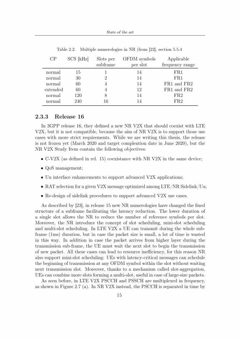
Differently from LTE RAT, where possible bandwidth blocks are just 1.4, 3,5, 10, 15 and 20 MHz, in 5G NR there are many channel bandwidth possibilitiesthanks to a flexible numerologies, or variable Sub-Carrier Spacing (SCS), fixed inLTE at 15 kHz, in 5g NR numerology changes. As stated in [21], a NR channelbandwidth is formed by a number of resource blocks, defined as "a consecutiveseries of 12 sub-carriers". Like in LTE numerology, in time domain radio framesare 10 ms long, composed by 10 subframes of 1 ms each. Nevertheless, in 5G NR inone subframe can fit one or more slots, depending on the sub-carrier spacing (SCS)as shown in [?]

Note that in case the cell has a large delay spread it is possible to use an extendedcyclic prefix for sub-carrier spacing equal to 60 kHz; in that case in one time slotit is possible to send just 12 OFDM symbols and not 14 as usual.

An important feature introduced is that in TDD operation, each OFDM symbolin a slot can be used in downlink, uplink or in a flexible manner: in other wordsthe scheduler can configure them semi-statically or dynamically.

14

State of the art

Table 2.2. Multiple numerologies in NR (from [22], section 5.5.4

CP SCS [kHz] Slots persubframe

OFDM symbolsper slot

Applicablefrequency range

normal 15 1 14 FR1normal 30 2 14 FR1normal 60 4 14 FR1 and FR2extended 60 4 12 FR1 and FR2normal 120 8 14 FR2normal 240 16 14 FR2

2.3.3 Release 16In 3GPP release 16, they defined a new NR V2X that should coexist with LTE

V2X, but it is not compatible, because the aim of NR V2X is to support those usecases with more strict requirements. While we are writing this thesis, the releaseis not frozen yet (March 2020 and target complention date in June 2020), but theNR V2X Study Item contain the following objectives:

• C-V2X (as defined in rel. 15) coexistance with NR V2X in the same device;

• QoS management;

• Uu interface enhancements to support advanced V2X applications;

• RAT selection for a given V2Xmessage optimized among LTE/NR Sidelink/Uu;

• Re-design of sidelink procedures to support advanced V2X use cases.

As described by [23], in release 15 new NR numerologies have changed the fixedstructure of a subframe facilitating the latency reduction. The lower duration ofa single slot allows the NR to reduce the number of reference symbols per slot.Moreover, the NR introduce the concept of slot scheduling, mini-slot schedulingand multi-slot scheduling. In LTE V2X a UE can transmit during the whole sub-frame (1ms) duration, but in case the packet size is small, a lot of time is wastedin this way. In addition in case the packet arrives from higher layer during thetransmission sub-frame, the UE must wait the next slot to begin the transmissionof new packet. All these cases can lead to resource inefficiency, for this reason NRalso support mini-slot scheduling: UEs with latency-critical messages can schedulethe beginning of transmission at any OFDM symbol within the slot without waitingnext transmission slot. Moreover, thanks to a mechanism called slot-aggregation,UEs can combine more slots forming a multi-slot, useful in case of large-size packets.

As seen before, in LTE V2X PSCCH and PSSCH are multiplexed in frequency,as shown in Figure 2.7 (a). In NR V2X instead, the PSCCH is separated in time by

15

State of the art

PSSCH: control information are sent before PSSCH transmission, so that a receivercan decode the message exactly when the transmission finish, not necessarily at theend of the sub-frame as in LTE V2X; in this way NR V2X can satisfy tighterlatency constraints. In Figure 2.7 (b) is illustrated the multiplexing in time, where,as [23] points out "the use of resources marked as "Idle/PSSCH" is still underconsideration and can be left idle or used for the transmission of PSSCH".

Figure 2.7. PSCCH and PSSCH in LTE V2X and NR V2X (from [23])

One key mechanism introduced in NR V2X is sidelink feedback channels. Evenif LTE V2X supports re-transmission, they are blind, or in other words, the retrans-mission are performed both in case the receiver effectively receive the packet or not.This re-transmission mechanism is fundamental to guarantee some reliability. Theintroduction of Physical Sidelink Feedback Channel (PSFCH) can provide higherchannel efficiency, higher channel state information leading to better reliability.

Like LTE V2X release 12, NR V2X defined 2 modes: the first one allow directcommunication within gNode B coverage, while the second mode support commu-nication completely independent from gNode B. Differently from previous releases,NR V2X Sidelink introduce new 4 sub-modes that distinguishes mode 2:

• Mode 2a: similarly with C-V2X sidelink mode 4, each UE selects its resourcesautonomously, considering sensed information;

• Mode 2b: UE can assist others to select resources, ;

• Mode 2c: UEs select resources using pre-configured grants;

16

State of the art

• Mode 2d: special UEs select resources for themselves and for other UEs, mainlyused for group communication for applications like platooning .

In further 3GPP meetings mode 2b and 2c are abandoned as separate sub-modesbecause mode 2b features can be used in modes 2a and 2d, while the pre-definedpatterns can be used in mode 2a.

What was thought in mode 2b - that can be exploited as well both in modes 2aand 2d - is the possibility by a user, for example the receiver, to notify the preferredresource elements using PSFCH. In mode 2a, every user can sense the PSFCH togather information about other UE preferred resource so that each user can choosethe best resources. The main limitation of this approach is high complexity in caseof high density scenario. In mode 2d a UE can perform resource allocation foritself and for the rest of the group. This sub-mode is useful in group applicationlike platooning. The user that perform resource allocation for the members of thegroup is called scheduling UE (S-UE). This mechanism is beneficial to the group,because it can reduce the number of collisions within the group. The main issue ofthis mode is the definition of S-UE: one proposal sees the S-UE be a pre-configuredvehicle, but this would imply additional hardware/processing capabilities for certainvehicles. Another proposal sees a geo-location based choice, in particular a vehiclein the middle of the group could have better radio information of all other membersof the platoon.

2.4 C-V2X schedulers

In order to meet requirements, one of the most important element in the trans-mission chain is the scheduler. In the following sections we describe the schedulerstandardized by 3GPP for LTE V2X mode 4 and some of our proposals that can beused as comparison to understand which one better fit the requirements for C-V2Xservices.

The first scheduler is called semi-persistent scheduler, while the others are theself organizing TDMA and the optical orthogonal codes.

2.4.1 Semi-Persistent Scheduling (SPS)

Because of periodicity and predictable packet size in V2X communication, 3GPPhas proposed a standardized scheduler called semi-persistent scheduling (SPS) thatis sensing-based. Its aim is to optimize the resource grid and minimize transmissioncollisions among different users.

As described in [24], in semi-persistent-scheduling every user transmits packetsin a certain slot every resource reservation interval (RRI). A counter is linkedwith each transmission and it is called SL_RESELECTION_COUNTER. Everytransmission this counter is reduced by one by the user MAC entity. When the

17

State of the art

counter reach zero, the user would reuse the same resource with probability pRK(probability resource keep) or would reselect a different resource with probability1 − pRK . In any case the user would extract an integer value randomly selectedamong the range C1 and C2 in uniform distribution. These two parameters dependsof course by the RRI value, according to Table 2.3. If the reselection choice is takenthe user generate some resource candidates inside the selection window.

Table 2.3. SL_RESELECTION_COUNTER range, depending on RRI value: [24]

RRI [C1, C2]

>= 100ms [5,15]50ms [10,30]20ms [25,75]

The selection window is a set of subframes in advance in respect of currentsubframe by T1 and T2. T1 depends on the user process delay, while T2 dependsfrom system requirements. Resource candidates are generated in function of whatwas sensed in the sensing window, whose length is of 1000 ms. The resource isselected uniformly randomly among the resource candidates.

In case two users selects the same time-frequency resource for transmission, thecollision cannot be avoided, but neither detected by either users. A bad feature ofthis scheduler is that in case of collision, it would persist over multiple messageswithout the user know about the collision. Furthermore, because of standardizedmessage frequencies, the probability of users select same messaging interval increase.For this reason the algorithm is not persistent but semi-persistent.

Analytical model and analysis In 2018, Manuel Gonzalez et al. published[25], where they explored the analytical model of C-V2X mode 4 and performancesfor a semi-persistent scheduler.

Initially the paper introduces the physical layer related to mode 4 and they itexplains the scheduling algorithm, defining variables like λ the packets transmittedper second per vehicle, the probability of reselection when the counter reach 0 pres aswell as dt,r: the distance among transmitter and receiver. Then the paper considerall possible sources of error and quantifies them probabilistically. δHD = Pr(e =HD) is the probability that the error come from half duplex impairment: this errorhappen when a user cannot receive a packet because that user was transmittingat that time slot. δSEN = Pr(e = SEN |e /= HD) is the probability that theerror is due to receiving power below a threshold PSEN , excluding half dupleximpairment. δPRO = Pr(e = PRO|e /= SEN, e /= HD) is the probability thatthe received power is higher that PSEN , the half duplex impairment is excluded,δCOL = Pr(e = COL|e /= PRO, e /= SEN, e /= HD) is the probability that another

18

State of the art

user has transmitted on the same time time slot, excluding the previous errors.The paper expands the previous formulas, exploring the sources of error. For

example the half duplex impairment depends just by the number of transmittedpackets by each vehicle and the number of sub-frames within a second,

δHD =λ

1000

Then, the sensing error

δSEN(dt,r) =1

2

(1− erf

(Pt − PL(dt,r)− PSEN

σ√2

))depends from the path loss and TX-RX distance, the transmitted power Pt and thereceiving power threshold PSEN .

δPRO(dt,r) =+ inf∑s=− inf

BL(s) · fSNR|Pr>PSEN ,dt,r(s)

where

fSNR|Pr>PSEN ,dt,r(s) =

{fSNR,dt,r

(s)

1−δSENa if Pr > PSEN

0 if Pr ≤ PSEN

is the PDF of the SNR experienced at a distance dt,r for values greater that PSEN ,and BL(s) is the BLER for SNR equal to s (these values come from look up tables).Finally the probability of error due to collision is

δCOL(dt,r) = 1−∏i

(1− δiCOL (dt,r, dt,i, di,r)

)where

δiCOL (dt,r, dt,i, di,r) = pSIM (dt,i) · pINT (dt,r, di,r)

is the probability of packet loss due to a collision with vehicle i, and it dependsfrom the probability that user i and user t transmit simultaneously on same re-sources and from probability that of interference with user i on the receiver, due tohigher received power from packet transmitted by user i in respect with that onetransmitter by user t.

Finally, in the paper this model has been validated by simulations in Veins andOMNET++, using SUMO for traffic simulation. The results state that the meanabsolute deviation of the model from the simulation is always below 2.5%, so themodel can be seen as valuable tool to further investigate behaviour of C-V2X mode4 under different scenarios and parameters.

19

State of the art

2.4.2 Self-organized Time Division Multiple Access (STDMA)Self-organizing TDMA (STDMA) is a protocol based on MAC layer. As stated

in [26], it is used in shipping (Automatic Identification System, AIS) and in airlinecompanies for his periodical structure. Because his tested on field effective, Eure-pean Telecommunication Standard Institute (ETSI) has considered STDMA a goodalternative to Carrier Sense Multiple Access with Collision Avoidance (CSMA/CA).

STDMA structure is composed by slot, whose dimensions, in terms of durationand bandwidth, depends from the fixed packet size. N slots form a frame, that isrepeated periodically in order to support periodical transmission. The parameter Ndepends from the application, from packet size and transmission parameters: fixedN, the channel capacity is determined. It is also assumed that all the users areslot-synchronized, but frame-synchronization is not required.

The STDMA protocol is based on slot reservation, so each user would transmitduring his slots time and would receive during the others slots. In order to avoidcollision, the protocol need to determine which slots each user can use to transmit.The protocol consists of four phases:

1. initialization phase;

2. network entry phase;

3. first frame phase;

4. continuous operation phase;

Initialization phase During the initialization phase, the selected user, beforeenter in the system, need to listen the channel for one entire frame and assign toevery slot a state depending on what they receive during each slot duration. Thelistening starting point depends from the user startup, so it is random. The possibleslot states are:

• Free slot;

• Internally allocated slot;

• Externally allocated slot;

• Unavailable slot.

Free: the slot is unused by any other user within range.Externally Allocated: the slot is used by an other one user within range, with apower level received above the Clear Channel Accessment (CCA) threshold.Internally Allocated: the slot is used or reserved by the current user.Unavailable: the slot is used by an other user but the received information cannotbe decoded correctly.

20

State of the art

Is important to notice that during the initialization phase, the state “internallyallocated” is impossible to find because no packets are scheduled yet. It must benoticed that a slot can be assigned the state “Unavailable” when a collision occur.We assume that the user during the following phases would continuously updatethe slot states, monitoring them during the receiving time. Once the selected userhas listened all the N slots and has assigned to each one a state, it follows withnetwork entry phase.

Network entry phase In network entry phase the current user should transmit aNetwork Entry Packet (NEP). This packet is sent just once and it’s aim is to informother users within range that a network joining is occurring. The NEP is trasmit ina free slot chosen randomly according to Random Access Time-Division MultipleAccess (RATDMA) protocol, because the slot is used without pre-annuntiation.In this phase two parameters are defined: the Candidate Set and Nominal Trans-mission Slot. The Candidate Set (CS) is the set of all free slots. The NominalTransmission Slots (NTS) is the set of slots chosen from the algorithm to actuallytransmit the packets, at this step it coincides with the NEP. The last part of thisphase is to choose the NTS among CS for the first transmission. In order to do sosome steps are required:a Nominal Increment (NI) is defined as NI = N/Rr the ideal interval between twoconsecutive packets;a Nominal Starting Slot (NSS) is defined and it is randomly chosen slot among CS;a Selection Interval (SI) is defined and it is the set of slots centred around NSS,whose cardinality depends from variable parameter s, that is the ratio of the lengthof SI and the length of NS and it is lower or equal to one.

After have defined SI, CS is compiled adding at first all free slots, then addingsome externally allocated slots in case the CS minimum size is not reached usingjust free slots. It has to be considered that externally allocated slots are addingstarting from those used by further users in respect of current user. Once definedCS, the NTS is chosen randomly with uniform probability over all CS. It mustbe noticed that in case the NTS correspond to an external allocated slot, somecollisions would be possible. Once the NTS is chosen, the user can transmit theNEP, adding the offset between the NEP slot and the NTS slot and it would enterin first frame phase.

First frame phase The main aim of first frame phase is to reserve all successiveNTS to satisfy the user communication. If the first packet was reserved by previousphase, the other r-1 NTSs must be decided before transmitting the first packet. Inthe first packet would be attached a timeout t0 to the NTS 0 and an offset to reservethe NTS 1. The timeout is used to reserve NTS 0 slot in the consecutive frames,so at every frame, at that timeslot, the timer would be decreased of one time unit.When it reaches 0, a new slot must be reserved according to procedures reported in

21

State of the art

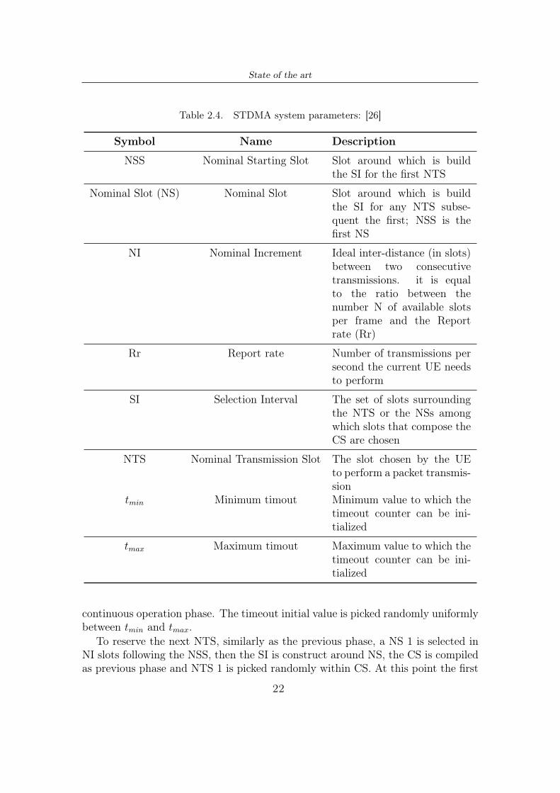
Table 2.4. STDMA system parameters: [26]

Symbol Name Description

NSS Nominal Starting Slot Slot around which is buildthe SI for the first NTS

Nominal Slot (NS) Nominal Slot Slot around which is buildthe SI for any NTS subse-quent the first; NSS is thefirst NS

NI Nominal Increment Ideal inter-distance (in slots)between two consecutivetransmissions. it is equalto the ratio between thenumber N of available slotsper frame and the Reportrate (Rr)

Rr Report rate Number of transmissions persecond the current UE needsto perform

SI Selection Interval The set of slots surroundingthe NTS or the NSs amongwhich slots that compose theCS are chosen

NTS Nominal Transmission Slot The slot chosen by the UEto perform a packet transmis-sion

tmin Minimum timout Minimum value to which thetimeout counter can be ini-tialized

tmax Maximum timout Maximum value to which thetimeout counter can be ini-tialized

continuous operation phase. The timeout initial value is picked randomly uniformlybetween tmin and tmax.

To reserve the next NTS, similarly as the previous phase, a NS 1 is selected inNI slots following the NSS, then the SI is construct around NS, the CS is compiledas previous phase and NTS 1 is picked randomly within CS. At this point the first

22

State of the art

packet is transmitted and it would contain the timeout t0 referring to NTS 0 overnext frames and the offset in slots from NTS 0 to NTS 1. Doing so, all the usersthat receive correctly the packet, can set the NTS 0 slot to the state externallyallocated, as well as the user would set it as internally allocated. This procedure isrepeated for r-1 times, until all r NTS are allocated. After the last transmission, theuser moves to the continuous operation phase. The picture section 2.4.2 representan example of first frame phase

Figure 2.8. STDMA parameters

Continuous operation phase The selected user enters in this phase when itis in steady state, so it has entered in the network, it has reserved his slot, itis aware of other user reservation and other users are aware of his reservationpattern. In this phase, the user transmits a packet in the NTS slot, decreasing theassociated timeout before the transmission. When the timeout reaches 0, a newNTS is reserved, following the same mechanism as before, and in the next packetit would be attached the offset and timeout associated.

It must be noticed that in this phase, the use of offset change from previousphase. If before it represented the number of slots for NTS i+1 from NTS i, inthis phase it indicates the offset related to the same NTS but in the next frame.In order to distinguish this two differences, the timeout is set to 0. So when thetimeout reach 0, the relative offset is reserving the NTS in the next frame.

Analytical model and analysis As seen in LTE physical layer description,the physical structure is characterized by several subchannel in frequency. Due toantenna limitation, a transmitting user is not able to sense the all the slots locatedat NTS slots.

This phenomenon is called by the authors “HD impairments” and due to thisphenomenon a new slot state must be introduced: hidden slot, that are those slot

23

State of the art

that cannot be received/sensed because located during user transmission. So a newsource of loss must be considered because of HD impairment, because of possiblecollisions.

In order to avoid HD effect we could extend the STDMA protocol into theOFDMA deployment (OSTDMA). The OSTDMA simply deal with possible colli-sions due to hidden slots removing these slots from CS during re-reservation def-inition. The current slot is however hold because other users would not select itbefore knowing the re-reservation parameters of the current NTS.

Figure 2.9. OFDM Self-organizing TDMA

This method uses a lot of resources, so it would work well when the channel loadis low, but in high channel load it would create collisions from other sources. Inorder to have better slot efficiency the author proposed the selective hiding STDMA(SH-STDMA). This second proposal assign a penalty to the SI higher if the distanceamong the user occupying a slot in the SI is nearer the receiver. In this way, whenthe CS must be compiled, free slots are added starting from subframes with lowerpenalties, or in other words, the algorithm selects slots externally allocated by usersthat are the furthest in mean from the receiver.

As expected the results in simulations shows that OSTDMA works better forlower channel load, but with higher channel load the SH-STDMA is better. So, in

24

State of the art

function of the channel load considered in the scenario, we choose one or the otherproposal.

2.4.3 OOC codesOptical Orthogonal Codes (OOC) are a family of (0,1) sequence that has some

special characteristics that were exploited for the first time in applications like codedivision multiple access (CDMA). It is possible to create a long set and then chunkit into (0,1) sequences called codewords. As described in [27], the codes satisfy theautocorrelation property and the cross-correlation property: the auto-correlation ofeach codeword in the OOC has a strong peak at τ = 0, and very low elsewhere andcross-correlation between any two sequences remains low. In particular given anypair of codewords u and v, from the same OOC set and with length L and given athreshold λ holds the following inequality:

L∑j=1

uj · vj ≤ λ ∀u /= v

Another important property of these codes is their periodic correlation, if wetake cyclic shift of codewords from an optical orthogonal codes, the correlationproperties are not affected.

The previous properties allow detection of desired signal reducing at minimumthe interference with unwanted signals in the medium. For this reason, opticalorthogonal codes are also used in those applications where low interference is akey element like mobile radio, radar and sonar signal design or frequency hoppingspread spectrum communications.

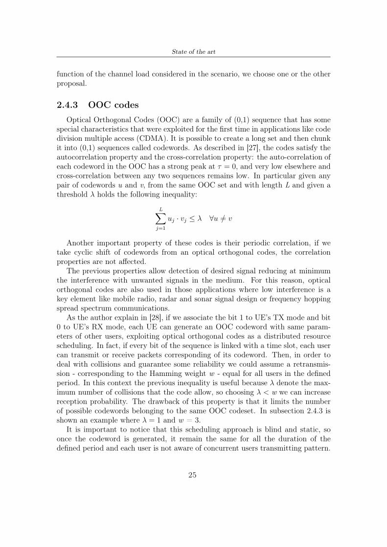
As the author explain in [28], if we associate the bit 1 to UE’s TX mode and bit0 to UE’s RX mode, each UE can generate an OOC codeword with same param-eters of other users, exploiting optical orthogonal codes as a distributed resourcescheduling. In fact, if every bit of the sequence is linked with a time slot, each usercan transmit or receive packets corresponding of its codeword. Then, in order todeal with collisions and guarantee some reliability we could assume a retransmis-sion - corresponding to the Hamming weight w - equal for all users in the definedperiod. In this context the previous inequality is useful because λ denote the max-imum number of collisions that the code allow, so choosing λ < w we can increasereception probability. The drawback of this property is that it limits the numberof possible codewords belonging to the same OOC codeset. In subsection 2.4.3 isshown an example where λ = 1 and w = 3.

It is important to notice that this scheduling approach is blind and static, soonce the codeword is generated, it remain the same for all the duration of thedefined period and each user is not aware of concurrent users transmitting pattern.

25

State of the art

Figure 2.10. Distributed allocation: OOC-based access to slots (from [28])

26

Chapter 3

Analytical study andsimulations

In this chapter we describe the scenario we have used in simulations. All param-eters are provided and all possible topologies are described, in such a way we candescribe how a perfect scheduler should perform, so that we can than compare withperformances given by semi-persistent scheduler and self-organizing time divisionmultiple access scheduler. After this theoretical analysis, we briefly introduce thenetwork simulator we have used. After the simulator description, we describe howthe workflow has been modified during the internship and which issues we haveencountered. After we expose simulation results both in NS3 and MATLAB, withcomments about results.

3.1 Perfect scheduler analysis

The scenario used is the depot, wherein we assumed 200 consists, organized in10 tracks with 20 consists each. Every track is spaced of 2 meters, each consist is26m long and spaced in respect to the next one 1 meter, for a total track length of269m. Each consist is 3 meters large.

The speed inside the depot is negligible, so that it can be excluded any significantDoppler effect, but path loss and shadowing effect have to be considered.

In the depot there are many consists, so high load is expected, and two phases:track creation, during which consist inside the same track as well as consists be-longing to different tracks would communicate, and track management where justconsist of the same track would communicate.

Exchanged packets are 1432 bits as packet size and they are transmitted every40ms.

There are two different possible topologies: mesh network and linear network.

27

Analytical study and simulations

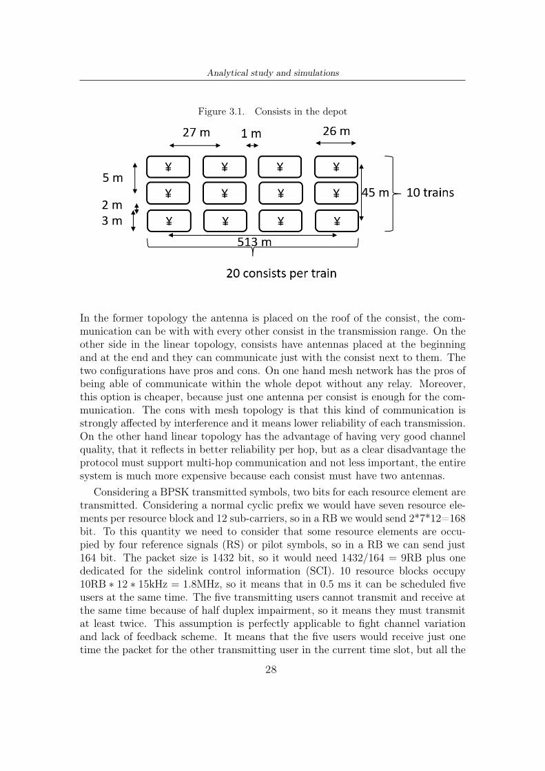
Figure 3.1. Consists in the depot

In the former topology the antenna is placed on the roof of the consist, the com-munication can be with with every other consist in the transmission range. On theother side in the linear topology, consists have antennas placed at the beginningand at the end and they can communicate just with the consist next to them. Thetwo configurations have pros and cons. On one hand mesh network has the pros ofbeing able of communicate within the whole depot without any relay. Moreover,this option is cheaper, because just one antenna per consist is enough for the com-munication. The cons with mesh topology is that this kind of communication isstrongly affected by interference and it means lower reliability of each transmission.On the other hand linear topology has the advantage of having very good channelquality, that it reflects in better reliability per hop, but as a clear disadvantage theprotocol must support multi-hop communication and not less important, the entiresystem is much more expensive because each consist must have two antennas.

Considering a BPSK transmitted symbols, two bits for each resource element aretransmitted. Considering a normal cyclic prefix we would have seven resource ele-ments per resource block and 12 sub-carriers, so in a RB we would send 2*7*12=168bit. To this quantity we need to consider that some resource elements are occu-pied by four reference signals (RS) or pilot symbols, so in a RB we can send just164 bit. The packet size is 1432 bit, so it would need 1432/164 = 9RB plus onededicated for the sidelink control information (SCI). 10 resource blocks occupy10RB ∗ 12 ∗ 15kHz = 1.8MHz, so it means that in 0.5 ms it can be scheduled fiveusers at the same time. The five transmitting users cannot transmit and receive atthe same time because of half duplex impairment, so it means they must transmitat least twice. This assumption is perfectly applicable to fight channel variationand lack of feedback scheme. It means that the five users would receive just onetime the packet for the other transmitting user in the current time slot, but all the

28

Analytical study and simulations

other receiving users would receive the packet twice.According to specification, each user would receive from higher layers a packet

to transmit periodically, it means that in that interval the scheduler must serveall users twice. In particular, following our scenario, every 0.5 ms the schedulercan allocate five users at the same time for 40 ms, it means that the scheduler has2slot per ms ∗ 40ms ∗ 5users = 400 time-frequency slots to assign. In the specificscenario, we should schedule 200 users, that transmitting two times need exactly400 transmission slots.

A perfect scheduler would allocate user according to the following scheme: if aslot is free allocate a new user in that slot and in the first free time-frequency slotin a time-set not yet occupied by any other users already scheduled in the currenttime-set. The Table 3.1 would better clarify the scheme: in the first time slot thefirst five users are allocated at different five sub-channels in the frequency domain,then in the second time slot other 4 users are scheduled and one user of the previousset is rescheduled, in such a way its information can be received by the four usersbelonging to the previous set. In the third time slot other three new users arescheduled plus one user of the first time slot set and one user of the second timeslot set and so on and so forth.

Table 3.1. Time frequency allocation in a perfect scheduler

1 1 2 3 4 52 6 6 7 8 93 7 10 10 11 124 8 11 13 13 145 9 12 14 15 15

It must be notices that the scheme would repeat exactly every 6 time-sets, soit means that if the total time-frequency slots is not a multiple of 6, some userscannot transmit twice. If we need to sacrifice some transmissions, the schedulercould avoid to send a message that a very far user has not received yet, becauseeven in case of transmission the further distance could effect the good receptionof the message anyway. For this purpose, the scheduler could assign a increasingnumber starting from users in the centre of the system and then at higher and higherdistances, such that the very last users that must be scheduled at the end of the 40ms are the furthest users. It must be considered that because of different receivedpower some messages cannot be decoded by all users, but for sake of simplicity wewould consider same received power at all receiving users. In the real world thisscheduler can be implemented in case an eNodeB would assign each user to eachtime-frequency slot. In that case the sidelink channel used would be the mode 3.This option is indeed probable because in a depot, there is the possibility of thepresence of a eNB.

29

Analytical study and simulations

In case the eNB is not present in the depot, all the consists must autonomouslycoordinate following a semi-persistent scheduler or a STDMA scheduler.

3.2 Network Simulator and workflowNS-3 is a discrete-event network simulator, targeted primarily for research and

educational use. NS-3 has been used because it allows users to run real implemen-tation code in the simulator.

Initially, one of the scopes of the internship was to upgrade some provided codeswritten in some older NS-3 versions, like NS-3.18 and NS-3.22 up to version NS-3.30. The main reason was that newer version provides more functionalities and thecorresponding simulations would have been more realistic. The main objective wasto have a stable newest version of the simulator, implementing LTE V2X feature.Upon that, the next step would be to change the LTE V2X scheduler and implementa different scheduler based on self-organizing time division multiple access.

The starting point was a NS-3.22 code of the implementation of LTE D2D, onthe same version a code implementing LTE V2X was provided. The workflow wasto start from the LTE V2X version and update it to version 30.

The first errors came by the new compiler: old codes are compiled by old com-pilers, but nowadays new compilers have more strict rules in order to prevent errorsinside the code. Other source of errors was that from past versions of network sim-ulator to version 30, many structures are changed, so during the compiling phase,many variables cannot be created because those structures did not exist any morein the new version of the simulator. Fixing these kind of errors were difficult be-cause sometimes some structures change radically where the simulator intended tosave variables, so we were stuck.

In the meanwhile, the national institute of standard technology website pub-lished a version of network simulator 3.30, implementing the LTE D2D. At thispoint, the workflow was modified: starting from NS-3.30 implementing LTE D2D,I would have to use the linux command diff among the two implementation ofLTE D2D and LTE V2X both in version 3.22, to generate the updated version ofLTE V2X running on network simulator version 30. Practically, we were meant tomodify the new code following the modifications were made in the older code toimplement the V2X feature. Diff command shown some changes in the two codes,like the scheduler, the physical layer module and some helper to deal with newobject that were created. For a better comprehension the Figure 3.2 explain themain objective. The main issue was that many modification were done on datastructure in the old simulator version that are no more existing in the new one ofthe simulator, so the most complex part was to understand which data structureswere change, how to apply modification from old data structures to new ones.

Unfortunately, these issues stole a lot of time and the limited duration of theinternship forces the workflow to redirect efforts in different direction again. The

30

Analytical study and simulations

Figure 3.2. Workflow representation

new aim of the internship became to investigate the semi-persistent scheduler inold version of NS-3.22 and compare the performances with the optical orthogonalcodes scheduler using an implementation in MATLAB as a simulation.

Indeed, as came from [26] and can be observed in Figure 3.3: in low channelload and very high channel load, optical orthogonal codes have better performancesthen STDMA. For this reason, it sounds reasonable explore how OOC performs inrespect with semi-persistent scheduling.

3.3 Simulations

For each simulation, the variation over density and inter-consist distance is anal-ysed, because the main scope is to observe if there is a possible scenario to meetrequirements. Moreover, a dedicated investigation over distribution is performed,in such a way to verify requirements in terms of probabilities. Furthermore, a vari-ation over different packet size is made to see if some observation can be made withthat parameter, both for fixed size or with variable packet size, following a gaussiandistribution and finally varying the modulation used.

3.3.1 Simulations using semi-persistent scheduler

The following simulations are performed considering a mesh topology, with an-tennas placed on top of the consist and being able to communicate with all othersantennas. The simulation select each consist as transmitter, and then sense the con-dition for every receiver, placed at a certain distance. When all consists are chosenas transmitter, the program estimate a mean value of parameters in function of

31

Analytical study and simulations

Figure 3.3. Comparison between STDMA and OOC taken from [26]

distance among transmitter and receiver.

Semi-persistent scheduling over density In figure 3.4 the first feature it canbe noticed is that independently by the simulation density, the performances don’tchange. This fact lead to the conclusion that the channel has enough capability tosustain all transmissions in the scenario.

The second important observation is about the points where distance is high:they do not follow the normal behaviour. The reason can be found in the so called"border effect". Indeed, the only consists that are so far apart are those at thelimit of the depot, and for those consists, the channel has more capacity, so theyhave better performances.

Another important observation must be done around network topology. Asdescribed before, the simulation are performed varying inter-antenna distances. Theantennas are thought to be placed on the top of the consists in a mesh topology, sothat all of them can communicate with every other consists. But as shown in 3.4,performances become very weak when the distance exceed half of the depot area.

32

Analytical study and simulations

Figure 3.4. PRR for different inter-antenna distance

Table 3.2. Conversion from density and inter-antenna distance

density [veh/hm2] inter-antenna distance [m]

87 444130 74180 37250 25500 172000 124000 9

Having this information in mind, seems reasonable to allow a multi-hop com-munication and reduce the antenna range capability. For example, if we wouldplace the antennas on consists like in a linear topology, antenna distance became10 meters. At that distance, the PRR is very high, so it would provide higherreliability.

Semi-persistent scheduling over distance In Figure 3.5 can be observed thatthe PRR is independent from density of antennas, but just the TX-RX distanceaffects performances. In other words, it means that the system can handle properlyall consists inside the depot, just shadowing effect and propagation affect transmis-sion in this configuration.

33

Analytical study and simulations

Figure 3.5. PRR over density for different TX-RX distance

Semi-persistent scheduling distribution probability InFigure 3.6 it is shownthe survival function of received packets, or in other words, it is shown the reli-ability of a packet to be received. In particular we have shown a density of 250veh/hm2, that corresponds to 200 consists in the depot, spaced by 2 meters amongconsists and 28 meters among consecutive antennas, in a mesh topology. If welook the reliability at a TX-RX distance of 10 m, we can see that we are sure thePRR is greater then 96%, but then the probability decrease quite fast. It must benoticed, that inter-consist distance is 2 meters, so if we observe from simulation atwhich point the probability degrade, it is around 99.95%. This quantity is still farfrom requirements for TSN, but it is a good improvements if we would use a lineartopology, in which antennas are placed in front and in the back of each consist, anda better per-hop communication can be reached.

Semi-persistent scheduling over different fixed packet size Considering afixed packet size, we can observe in Figure 3.7 that we have same performancesfor some packet dimensions. As we can see, just three lines are shown because theothers are overwritten, as they are exactly the same. So packet size of 15 bytes and50 bytes have the same performances of a size of 100 bytes, then 179, 200 and 300bytes have the same performances. This behaviour can be explained by the factthat some padding is inserted inside a packet, so until the size doesn’t reach thethreshold, performances doesn’t change. This behaviour is important to observebecause if the packet size is around the padding threshold, it can be considered toreduce a bit of information in order to get higher performances, or in the opposite

34

Analytical study and simulations

Figure 3.6. Reliability for density at 250veh/hm2 and TX-RX distance at 10m

case, include more information that would not affect the transmission.

Semi-persistent scheduling over variable packet size It is possible that thesystem may work with fixed packet size, but sounds reasonable that the applicationsends some small packets as well as big packets. For this reason we have studied thebehaviour of the system, in case of a variable packet size, statistically distributedas a gaussian with mean equal to 340 bytes and a standard deviation of 100 bytes.In other words, the 95% of packet sizes are between 140 and 540 bytes. Results areshown in Figure 3.8.

We can observe that for short distance the system has very high probability ofreception: 99.9% for distance before 15 meters. then it slowly decrease to 99% until200 meters and then decrease steeply. The steep decrease at 200 m is reasonablelooking at the behaviour for fixed packet size at 300 bytes, but what is much betterfor variable packet size is the performance for lower distances, that before wasaround 99% for small packet size and small distance.

3.3.2 Simulations using optical orthogonal codes

In the following sections we describe the behaviour of the system using opticalorthogonal codes in conditions as similar as possible to previous scenario, in order tobe comparable. Unfortunately, the codes are extremely different so some differencemust be reported.

First of all, the scenario is no more a 2D depot, but it is more a 1D line, whereone transmitter at the centre of the line send a message, and all the consists inside

35

Analytical study and simulations

Figure 3.7. PRR for different packet size

the receiving range receive it. The receiving range is the same as the depot scenario:the hypotenuse of the 2D depot whose length is 514 m.

Secondly, the code just test the behaviour of the system at layer 2, so the physicallayer is completely ignored, that’s why, as we describe later, the performance doesnot change over distance: no path loss or shadowing effects are considered, but justcollisions.

It must be noticed that all consists in the range, check if the transmitting slotcorresponds to a slot already occupied by other consists - this case would lead toa collision - or occupied by themselves - leading not to receiving it because of halfduplex hiding.

Lastly, because this is a linear topology, the density is specify in vehicles/km,differently as before, but the number of vehicles in the system remain compatiblewith previous scenario.

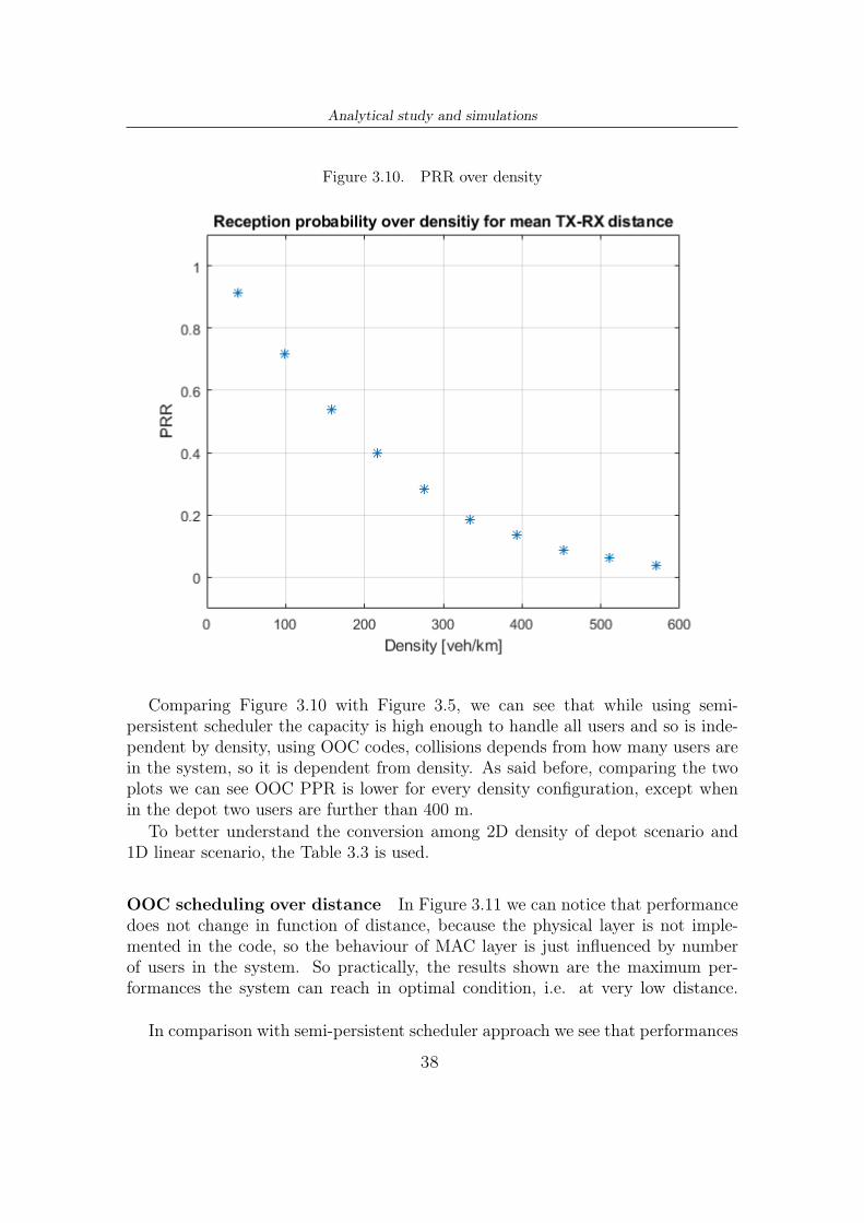
OOC scheduling over density Regarding Figure 3.10, the first observation isabout how the system reacts when we change the density. As we can see, the PRR

36

Analytical study and simulations

Figure 3.8. PRR over gaussian distributed packet size

Figure 3.9. Consists in the linear depot

decrease like an exponential.A second observation is that even in the best possible condition the OOC ap-

proach reach at maximum 90% of reception probability due to collision and halfduplex impairment.

37

Analytical study and simulations

Figure 3.10. PRR over density

Comparing Figure 3.10 with Figure 3.5, we can see that while using semi-persistent scheduler the capacity is high enough to handle all users and so is inde-pendent by density, using OOC codes, collisions depends from how many users arein the system, so it is dependent from density. As said before, comparing the twoplots we can see OOC PPR is lower for every density configuration, except whenin the depot two users are further than 400 m.

To better understand the conversion among 2D density of depot scenario and1D linear scenario, the Table 3.3 is used.

OOC scheduling over distance In Figure 3.11 we can notice that performancedoes not change in function of distance, because the physical layer is not imple-mented in the code, so the behaviour of MAC layer is just influenced by numberof users in the system. So practically, the results shown are the maximum per-formances the system can reach in optimal condition, i.e. at very low distance.

In comparison with semi-persistent scheduler approach we see that performances

38

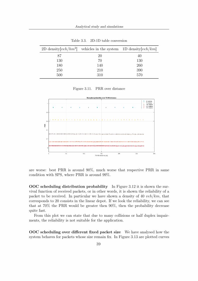
Analytical study and simulations

Table 3.3. 2D-1D table conversion

2D density[veh/hm2] vehicles in the system 1D density[veh/km]

87 20 40130 70 130180 140 260250 210 390500 310 570

Figure 3.11. PRR over distance

are worse: best PRR is around 90%, much worse that respective PRR in samecondition with SPS, where PRR is around 99%.

OOC scheduling distribution probability In Figure 3.12 it is shown the sur-vival function of received packets, or in other words, it is shown the reliability of apacket to be received. In particular we have shown a density of 40 veh/km, thatcorresponds to 20 consists in the linear depot. If we look the reliability, we can seethat at 70% the PRR would be greater then 90%, then the probability decreasequite fast.

From this plot we can state that due to many collisions or half duplex impair-ments, the reliability is not suitable for the application.

OOC scheduling over different fixed packet size We have analysed how thesystem behaves for packets whose size remain fix. In Figure 3.13 are plotted curves

39

Analytical study and simulations

Figure 3.12. Reliability for density at 70veh/km

at different densities, depending on packet size. We can see that the PRR decreaseexponentially, increasing with packet size, but for small packets the curve tends tobe almost linear.

The best possible performance is when we have low packet size and few consistsin the depot, reaching a PRR around 99%.

Comparing with the corresponding plot using semi-persistent scheduler, we cansee that OOC approach is worse

OOC scheduling over variable packet size In Figure 3.14 is shown the be-haviour of the system, when packets are not all the same, but they have differentsizes, distributed as a gaussian, with mean equal to 200 and standard deviationequal to 80. This means that 95% of packets have size between 40 and 360 bytes.

These values are a lower than the corresponding plots of semi-persistent sched-uler, but in this case the mean value is much closer to system packet size: 179bytes.

We can immediately observe that PRR does not depend from distance, but it

40

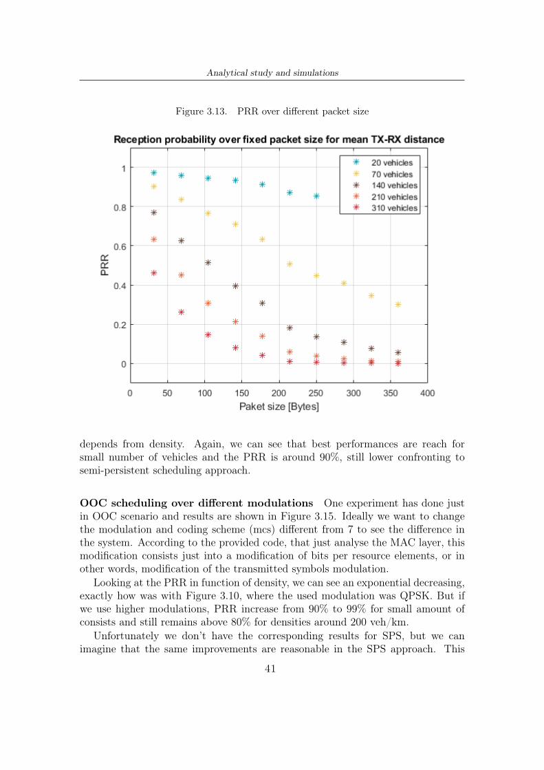
Analytical study and simulations

Figure 3.13. PRR over different packet size

depends from density. Again, we can see that best performances are reach forsmall number of vehicles and the PRR is around 90%, still lower confronting tosemi-persistent scheduling approach.

OOC scheduling over different modulations One experiment has done justin OOC scenario and results are shown in Figure 3.15. Ideally we want to changethe modulation and coding scheme (mcs) different from 7 to see the difference inthe system. According to the provided code, that just analyse the MAC layer, thismodification consists just into a modification of bits per resource elements, or inother words, modification of the transmitted symbols modulation.

Looking at the PRR in function of density, we can see an exponential decreasing,exactly how was with Figure 3.10, where the used modulation was QPSK. But ifwe use higher modulations, PRR increase from 90% to 99% for small amount ofconsists and still remains above 80% for densities around 200 veh/km.

Unfortunately we don’t have the corresponding results for SPS, but we canimagine that the same improvements are reasonable in the SPS approach. This

41

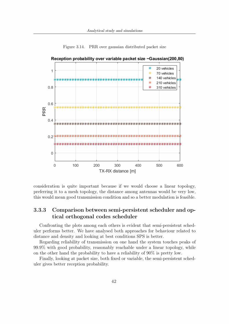
Analytical study and simulations

Figure 3.14. PRR over gaussian distributed packet size

consideration is quite important because if we would choose a linear topology,preferring it to a mesh topology, the distance among antennas would be very low,this would mean good transmission condition and so a better modulation is feasible.

3.3.3 Comparison between semi-persistent scheduler and op-tical orthogonal codes scheduler

Confronting the plots among each others is evident that semi-persistent sched-uler performs better. We have analysed both approaches for behaviour related todistance and density and looking at best conditions SPS is better.

Regarding reliability of transmission on one hand the system touches peaks of99.9% with good probability, reasonably reachable under a linear topology, whileon the other hand the probability to have a reliability of 90% is pretty low.

Finally, looking at packet size, both fixed or variable, the semi-persistent sched-uler gives better reception probability.

42

Analytical study and simulations

Figure 3.15. PRR over different modulation

43

Chapter 4

Conclusion and future work

After having analysed the behaviour of the system and having appreciated thecomparison between the two proposed algorithms, in this final chapter we drawconclusions about our experiments and we describe what will experiment next, tobetter research on this field, to reach our objectives.

4.1 Conclusion

We have analysed many system parameters in order to look at some perfor-mances, but for both tested schedulers we are still quite far from requirements fortime sensitive networks. Nevertheless, there are some important results that wecan remember.

The most important one is the 0.999 reliability in a transmission at 10 meters.This results assure a good condition transmission per hop in a linear topology.Linear topology would imply more packets to send and multi-hop problem, but incase these problems would find solution, per hop conditions are good.

The second observation that we can make is the obvious superiority of semi-persistent scheduler with respect to optical orthogonal codes. This can be ex-plained because OOC assign slots to users without considering the users already inthe channel, while semi-persistent approach sense the channel before choosing thetransmitting slots.

Finally we need to observe that when transmission conditions are good we couldimprove performances increasing the modulation, and even considering a variablepacket size could be beneficial for the system, because even if the behaviour inmean remain the same, it is better for lower distances and lower densities.

44

Conclusion and future work

4.2 Future worksThis thesis analyses performaces of OOC algorithm simulated in MATLAB. The

next step would be looking at the same experiments using an STDMA scheduler inMATLAB, to see if performances increase in respect to semi-persisten scheduler. Ifso, would be better to have the same scheduler in NS3 environment and simulate thescenario in a full stack implementation, comparing results with the correspondingusing semi-persistent scheduler. After the NS3 simulation, the next interestingstep would be implementing the STDMA scheduler in Open Air Interface (OAI)and emulate the scenario first in the emulator environment, then test the schedulerdeploying the code directly in real world.

Finally, in March 2020 the 3GPP release 16 would be frozen and physical layerwould be specified, as well as the scheduler: an interesting comparison would beapplying STDMA or semi-persistent scheduler on 5G physical layer and comparingit with the standardized scheduler.

45

Bibliography

[1] “Saving lives: Boosting car safety in the EU.” https://eur-lex.europa.eu/legal-content/EN/TXT/HTML/?uri=CELEX:52016DC0787&from=EN.

[2] “Self driving cars in the EU.” https://www.europarl.europa.eu/news/en/headlines/economy/20190110STO23102/self-driving-cars-in-the-eu-from-science-fiction-to-reality.

[3] “Safe 4 RAIL 2 project.” www.safe4rail.eu.[4] G. Naik, B. Choudhury, and J.-M. Park, “Ieee 802.11bd and 5g nr v2x: Evo-

lution of radio access technologies for v2x communications,” IEEE Access,vol. PP, pp. 1–1, 05 2019.

[5] A. Jovicic, J. Li, and T. Richardson, “Visible light communication: opportu-nities, challenges and the path to market,” IEEE Communications Magazine,vol. 51, pp. 26–32, December 2013.

[6] S. Ishihara, R. V. Rabsatt, and M. Gerla, “Improving reliability of platooningcontrol messages using radio and visible light hybrid communication,” in 2015IEEE Vehicular Networking Conference (VNC), pp. 96–103, Dec 2015.

[7] A. Nasrallah, A. S. Thyagaturu, Z. Alharbi, C. Wang, X. Shao, M. Reisslein,and H. ElBakoury, “Ultra-low latency (ull) networks: The ieee tsn and ietfdetnet standards and related 5g ull research,” IEEE Communications SurveysTutorials, vol. 21, pp. 88–145, Firstquarter 2019.

[8] “Time sensitive networking (tsn) task group.” https://1.ieee802.org/tsn.[9] “Ls on 3gpp 5g system support for integration with ieee tsn

networks.” http://www.ieee802.org/1/files/public/docs2019/liaison-3gppsa2-1908630-5g-integration-with-tsn-0719.pdf.

[10] A. Z. Hindi, S. Elayoubi, and T. Chahed, “Performance evaluation of ultra-reliable low-latency communication over unlicensed spectrum,” in ICC 2019 -2019 IEEE International Conference on Communications (ICC), pp. 1–7, May2019.

[11] C. Stefanovic, “Industry 4.0 from 5g perspective: Use-cases, requirements, chal-lenges and approaches,” in 2018 11th CMI International Conference: Prospectsand Challenges Towards Developing a Digital Economy within the EU, pp. 44–48, Nov 2018.

46

Bibliography

[12] E. G. Ström, P. Popovski, and J. Sachs, “5g ultra-reliable vehicular communi-cation,” CoRR, vol. abs/1510.01288, 2015.

[13] “Industrial wireless time-sensitive networking: Rfc on the pathforward.” https://avnu.org/wp-content/uploads/2014/05/Industrial-Wireless-TSN-Roadmap-v1.0.3-1.pdf.

[14] Time Sensitive Networking for Wireless Networks-A State of the Art Analysis,2019.

[15] “D2.6–wireless consist network report.” http://www.ieee802.org/1/files/public/docs2019/liaison-3gppsa2-1908630-5g-integration-with-tsn-0719.pdf.

[16] [TS 23.303], "Technical Specification Group Services and System Aspects; Prox-imity -based services (ProSe); Stage 2", 3gpp ts 23.303 v13.2.0 ed., 12/2015.

[17] [TS 36.331], "Technical Specification Group Radio Access Network; EvolvedUniversal Terrestrial Radio Acess (E-UTRA); Radio Resource Control (RCC);Protocol specification", 3gpp ts 36.331 v13.0.0 ed., 12/2015.

[18] [TS 36.300], "Evolved Universal Terrestrial Radio Access (E-UTRA) andEvolved Universal Terrestrial Radio Access Network (E-UTRAN); Overall de-scription; Stage 2", 3gpp ts 36.300 v13.3.0 ed., 4/2016.

[19] [TS 22.185], "Technical Specification Group Services and System Aspects; Ser-vice requirements for V2X services; Stage 1", 3gpp ts 22.185 v15.0.0 ed.,6/2018.

[20] “3gpp v2x overview.” https://www.3gpp.org/v2x.[21] [TR 21.915], "Technical Specification Group Services and System Aspects;

Release 15 Description; Summary of Rel-15 Work Items", 3gpp tr 21.915v15.0.0 ed., 9/2019.

[22] [TR 22.186], "Technical Specification Group Services and System Aspects; En-hancement of 3GPP support for V2X scenarios", 3gpp tr 22.186 v16.2.0 ed.,6/2019.

[23] G. Naik, B. Choudhury, and J. Park, “Ieee 802.11bd 5g nr v2x: Evolutionof radio access technologies for v2x communications,” IEEE Access, vol. 7,pp. 70169–70184, 2019.

[24] N. Bonjorn, F. Foukalas, and P. Pop, “Enhanced 5g v2x services using sidelinkdevice-to-device communications,” in 2018 17th Annual Mediterranean Ad HocNetworking Workshop (Med-Hoc-Net), pp. 1–7, June 2018.

[25] M. Gonzalez-Martín, M. Sepulcre, R. Molina-Masegosa, and J. Gozalvez, “An-alytical models of the performance of c-v2x mode 4 vehicular communications,”IEEE Transactions on Vehicular Technology, vol. 68, pp. 1155–1166, Feb 2019.

[26] L. Gallo and J. Härri, “Self organizing tdma over lte sidelink,” Tech. Rep.RR-5105, 2017.

[27] F. R. K. Chung, J. A. Salehi, and V. K. Wei, “Optical orthogonal codes: design,analysis and applications,” IEEE Transactions on Information Theory, vol. 35,pp. 595–604, May 1989.

47

Bibliography

[28] L. Gallo, Medium access control for cellular-based vehicular ad-hoc networks.PhD thesis, Thesis, 05 2017.

48