semiactive coulomb friction lead–lag dampers€¦ · dissipation characteristics of the device...

JOURNAL OF THE AMERICAN HELICOPTER SOCIETY 55, 012005 (2010)

Semiactive Coulomb Friction Lead–Lag Dampers

Olivier A. Bauchau∗ Yannick Van Weddingen Sandeep AgarwalDaniel Guggenheim School of Aerospace Engineering, Georgia Institute of Technology, Atlanta, GA

Lead–lag dampers are present in most rotor systems to provide the desired level of damping for all flight conditions. These

dampers are critical components of the rotor system and also represent a weight and drag penalty together with a major

source of maintenance costs. The performance of semiactive Coulomb friction based lead–lag dampers is examined in this

study. First, conceptual designs of semiactive friction dampers for rotorcraft applications are briefly presented. Next, the

concept of adaptive damping is discussed: by adjusting the normal contact force at the frictional interface, the energy

dissipation characteristics of the device can be tailored, providing “damping on demand.” The behavior of friction dampers

in both ground resonance and forward flight is simulated for the UH-60 aircraft and compared with that of present hydraulic

dampers. The approach used for modeling the frictional process is presented in detail. The final part of this paper explores

the concept of selective damping, in which the energy dissipation capacity of semiactive devices is targeted to a specific

mode. Practical implementation of this concept is shown to face many challenges.

Introduction

Although it would be most desirable to completely eliminate lead–lag dampers from articulated helicopter rotor systems, this ideal goalremains elusive despite significant research in this area. Designs havebeen proposed that eliminate the need for lead–lag dampers in groundresonance or air resonance cases, but designs that achieve both goalssimultaneously have not been fully satisfactory (Refs. 1–6). Furthermore,lead–lag damping is also required during maneuvering flight, such asdescent flight conditions. Consequently, lead–lag dampers are found onmany rotor systems despite the added mechanical complexity and cost.Hydraulic dampers are complex mechanical components that requirethe use of hydraulic fluids in the rotating system. This results in highmaintenance costs to prevent oil leaks and subsequent failure. Moreover,internal seal failures can reduce damping in the device with no externalsigns of leakage. Elastomeric dampers are conceptually simpler andprovide a “dry rotor,” but their damping characteristics can degrade dueto temperature and stress cycling, thus resulting in high maintenancecost. More often than not, this degradation occurs without external signsof failure, and hence dampers must be replaced on a regular basis, furthercontributing to the high cost of ownership of the device. It should alsobe noted that elastomeric dampers present a certain stiffness associatedwith the inherent stiffness of the material. This stiffness changes the rotordynamic characteristics, and hence the damper becomes an integral partof the rotor system.

The hydraulic and elastomeric lead–lag dampers described in theprevious paragraph are usually passive devices. More often than not,dampers are designed to provide sufficient damping for the most critical

∗Corresponding author; e-mail: [email protected] received December 2007; accepted August 2009.

flight conditions, typically ground resonance and violent maneuvers. Forpassive devices, this damping level and the associated damping forceswill then be present at all flight conditions, whether required or not. Inmany cases, the required level of damping in forward flight might besignificantly lower than that required in ground resonance; yet, when apassive device is used, the same damping level will be present throughoutthe flight envelope. In forward flight, dampers will experience large 1Pmotions due to Coriolis and drag forces, resulting in large damper forces;since 1P motions will not lead to an instability, these large damping forcesmight not be necessary, although contributing to fatigue of the damperand connected components. This problem was recognized in the designof hydraulic lead–lag dampers. The hydraulic damper of the UH-60helicopter, for instance, features a pressure relief valve that limits thedamper force to a preset level for high stroking velocity. While suchhydraulic damper remains a passive device, it clearly features an attemptto achieve “damping on demand,” i.e., the tailoring of the amount ofdamping provided by the device to the required damping level.

The concept of “adaptive damping” or “damping on demand” takes onnew dimensions when semiactive devices are used as rotorcraft lead–lagdampers. In semiactive devices, actuation is used to modify the phys-ical characteristics of a passive element. This is to be contrasted withactive devices, for which controlled actuation forces are directly appliedto the system. For instance, the use of semiactive, magnetorheologicalfluid dampers was explored by Gandhi et al. (Refs. 7, 8) and Zhao et al.(Ref. 9). In this concept, the lead–lag damper is a hydraulic device featur-ing a magnetic particle laden fluid. A magnetic field is used to change therheological properties of the fluid, thereby adjusting damping levels tomeet the requirement for a specific flight condition. Further investiga-tions, such as in Ref. 10, have been done including magnetorheologicalfluid devices in more advanced damper designs. In this work, a differentconcept is investigated: Coulomb friction forces will be used to provide

DOI: 10.4050/JAHS.55.012005 C© 2010 The American Helicopter Society012005-1

O. A. BAUCHAU JOURNAL OF THE AMERICAN HELICOPTER SOCIETY

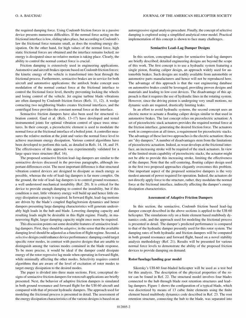
the required damping force. Using Coulomb friction forces in a passivedevice presents numerous difficulties. If the normal force acting on thefrictional interface is low, sliding takes place, but according to Coulomb’slaw the frictional force remains small, as does the resulting energy dis-sipation. On the other hand, for high values of the normal force, highstatic frictional forces are obtained and the interface remains locked; noenergy is dissipated since no relative motion is taking place. Clearly, theability to control the normal contact force is crucial.

Friction damping is extensively used in engineering applications.Automotive and aircraft brakes operate based on Coulomb friction forces:the kinetic energy of the vehicle is transformed into heat through thefrictional process. Furthermore, semiactive brakes are in service for bothaircraft and automotive applications: the antilock brake concept usesmodulation of the normal contact force at the frictional interface tocontrol the frictional force level, thereby preventing locking the wheelsand losing control of the vehicle. Jet engine turbine blade vibrationsare often damped by Coulomb friction forces (Refs. 11, 12). A wedgecontacting two neighboring blades creates frictional interfaces, and thecentrifugal force provides the constant normal force at the interface.

Semiactive friction dampers have also been used for structural vi-bration control. Gaul et al. (Refs. 13–17) have developed and testedinstrumented joints for optimal vibration control of space truss struc-tures. In their concept, a piezoelectric element is used to modulate thenormal force at the frictional interface of a bolted joint. A controller mea-sures the relative motion at the joint and varies the normal force level toachieve maximum energy dissipation. Various control algorithms havebeen developed to perform this task, as detailed in Refs. 14, 18, and 19.The effectiveness of this approach was experimentally validated for alarge space truss structure (Ref. 16).

The proposed semiactive friction lead–lag dampers are similar to thesemiactive devices discussed in the previous paragraphs, although im-portant differences exist. The most important difference is that structuralvibration control devices are designed to dissipate as much energy aspossible, whereas the role of lead–lag dampers is far more complex. Onthe ground, the role of lead–lag dampers is to control ground resonance,a well understood mechanical instability (Ref. 20). It is critical for thedevice to provide enough damping to control the instability, but if thiscondition is met, little vibratory energy will build up and hence little en-ergy dissipation capacity is required. In forward flight, lead–lag motionsare driven by the blade’s coupled flap/lag/torsion dynamics and hencedampers presenting large damping characteristics will generate undesir-ably high loads in the hub and blade. Lowering damping capacity andresulting loads might be desirable in this flight regime. Finally, in ma-neuvering flight, larger damping capacity might once more be required.

This discussion points out some desirable features of semiactive lead–lag dampers. First, they should be adaptive, in the sense that the availabledamping level should be adjusted as a function of flight regime. Second, aselective design could enhance device performance: damping could targetspecific rotor modes, in contrast with passive designs that are unable todistinguish among the various modes contained in the blade response.To be more precise, it would be ideal if the damper could dissipateenergy of the rotor regressive lag mode when operating in forward flight,while minimally affecting the other modes. Selectivity requires controlalgorithms that are aware of the level of excitation of rotor modes totarget energy dissipation to the desired modes.

The paper is divided into three main sections. First, conceptual de-signs of semiactive friction dampers for rotorcraft applications are brieflypresented. Next, the behavior of adaptive friction dampers is simulatedin both ground resonance and forward flight for the UH-60 aircraft andcompared with that of present hydraulic dampers. The approach used formodeling the frictional process is presented in detail. The assessment ofthe energy dissipation characteristics of the various designs is based on an

autoregressive signal analysis procedure. Finally, the concept of selectivedamping is explored using a simplified analytical rotor model. Practicalimplementation of this concept is shown to face many challenges.

Semiactive Lead–Lag Damper Designs

In this section, conceptual designs for semiactive lead–lag dampersare briefly described; detailed engineering designs are beyond the scopeof this work. The first concept is to use a hydraulic system featuring asingle piston, floating caliper design, an approach widely used for au-tomobile brakes. Such designs are readily available from automobile orautomotive parts manufacturers and hence will not be reproduced here.The advantage of this approach is that the vast engineering databaseon automotive brakes could be leveraged, providing proven designs andmaterials and leading to low-cost devices. The disadvantage of this ap-proach is that it requires the use of hydraulic lines in the rotating system.However, since the driving piston is undergoing very small motions, nodynamic seals are required, drastically limiting leaks.

In an effort to avoid hydraulic systems, the second concept uses anelectric motor to actuate a floating caliper design similar to that used inautomotive brakes. The last concept relies on piezoelectric actuation: Aset of piezoelectric stack actuators provides the required normal force atthe friction interface, generating the desired friction force. The actuatorswork in compression at all times, a requirement for piezoelectric stacks.The advantage of these last two approaches is the electric actuation: theseare “dry dampers.” A number of disadvantages stem from the limitationsof piezoelectric actuation. Indeed, as wear develops at the frictional inter-face, an increasing stroke will be required of the stack actuators. In viewof the limited strain capability of piezoelectric stacks, the actuator mightnot be able to provide this increasing stroke, limiting the effectivenessof the damper. Note that the self-centering, floating caliper design usedin the first two proposed approaches elegantly overcomes this problem.One important aspect of the proposed semiactive dampers is the verymodest amount of power required for operation. Indeed, the actuators donot directly apply force to the structure, rather, they modulate the normalforce at the frictional interface, indirectly affecting the damper’s energydissipation characteristics.

Assessment of Adaptive Friction Dampers

In this section, the semiactive, Coulomb friction based lead–lagdamper concept described in the above sections is applied to the UH-60helicopter. The simulations rely on a finite element based multibody dy-namics code, and the approach used for modeling the frictional processis presented in detail. The damper’s predicted performance is comparedto that of the hydraulic damper presently used for this rotor system. Thedamping rates of both hydraulic and friction dampers will be computedin both ground resonance and forward flight, based on a novel stabilityanalysis methodology (Ref. 21). Results will be presented for variousnormal force levels to demonstrate the ability of the proposed frictiondevices to provide damping on demand.

Rotor/fuselage/landing gear model

Sikorsky’s UH-60 four-bladed helicopter will be used as a test bedfor this analysis. The description of the physical properties of the ro-tor can be found in Ref. 22. The structural model involves four bladesconnected to the hub through blade root retention structures and lead–lag dampers. Figure 1 shows the configuration of a typical blade, whichwas discretized by means of 13 cubic finite elements using the finiteelement based multibody dynamics code described in Ref. 23. The rootretention structure, connecting the hub to the blade, was separated into

012005-2

SEMIACTIVE COULOMB FRICTION LEAD–LAG DAMPER 2010

Fig. 1. UH-60 rotor system with the proposed semiactive Coulomb

friction lead–lag damper.

three segments labeled segment 1, 2, and 3, respectively, in Fig. 1. Thefirst segment, modeled by one beam element, was attached to the hub.The flap, lead–lag, and pitch hinges of the blade were modeled by threerevolute joints connecting the first two segments of the root retentionstructure. The physical characteristics of the elastomeric bearing wererepresented by springs and dampers in the joints to model the stiffnessand energy dissipation characteristics of the elastomeric material. Theouter two segments, each modeled by two beam elements, were rigidlyconnected to each other and to the pitch horn. Finally, the outermost seg-ment was rigidly connected to the blade and damper horn. The pitch angleof the blade was set by the following control linkages: the swashplate,pitch link, and pitch horn. The pitch link, modeled by three cubic beamelements, was attached to the rigid swashplate by means of a universaljoint and to the rigid pitch horn by a spherical joint. The damper armand damper horn were modeled as rigid bodies. The lead–lag damperwas modeled as a prismatic joint; its end points were connected to thedamper arm and horn. Since the kinematics of the damper are accuratelymodeled, all kinematic couplings between blade and damper motions aretaken into account.

For forward flight simulations, the hub of the rotor model described inthe previous paragraph was connected to the ground; fuselage dynamicswas therefore ignored in this case. For ground resonance simulations, thesame rotor model was connected to the fuselage, represented by a rigidbody with appropriate mass and moment of inertia characteristics. Thelanding gear consists of three supporting structures: the left, right, andtail gears, respectively. Each gear includes an oleo strut and tire. The oleostruts were modeled as prismatic joints connected to the fuselage centerof mass and to the tires. The axis of each prismatic joint was properlyaligned with the axis of the corresponding strut, and a combinationincluding springs and a linear dashpot was added to each prismatic jointto model the characteristics of the two-stage oleo device. The tires weremodeled by a set of linear springs and dashpots connected to the ground.Each tire features three spring stiffness constants: one constant for motionin the direction perpendicular to the ground plane and two constants formotions in the ground plane. Additional information and data about thefixed system model can be found in Refs. 24 and 25.

Friction modeling

An important aspect of the present work is the modeling of the frictiondampers. From a kinematics standpoint, the damper is modeled as aprismatic joint, which allows the relative displacement, �, of the twosides of the joint along a prescribed direction in the material frame,n. The normal force at the frictional interface is denoted f n, a time-dependent user input. The friction model described later then evaluatesthe magnitude of the frictional force, which is applied as equal andopposite forces on the two sides of the joint, providing full couplingbetween the frictional process and the system dynamic response.

The detailed modeling of frictional forces poses unique computa-tional challenges that will be illustrated using Coulomb’s law as anexample. When sliding takes place, Coulomb’s law states that the fric-tion force, F f , is proportional to the magnitude of the normal force,F f = −μk(v) f n sign(v), where μk(v) is the coefficient of kinetic fric-tion and v = � the magnitude of the relative velocity vector at theprismatic joint. Both friction force and relative displacement are posi-tive in the direction of n. If the relative velocity vanishes, sticking takesplace. In this case, the frictional force is |F f | ≤ μs f n, where μs is thecoefficient of static friction.

Application of Coulomb’s law involves discrete transitions from stick-ing to sliding and vice versa, as dictated by the vanishing of the relativevelocity or the magnitude of the friction force. These discrete transitionscan cause numerical difficulties that are well documented, and numerousauthors have advocated the use of a continuous friction law (Refs. 26–28)typically written as

F f = −μk(v) f n sign(v) (1 − e−|v|/v0 ) (1)

where (1−e−|v|/v0 ) is a “regularization factor” that smoothes out the fric-tion force discontinuity and v0 a characteristic velocity usually chosen tobe small compared to the maximum relative velocity encountered duringthe simulation. The continuous friction law describes both sliding andsticking behavior, i.e., it completely replaces Coulomb’s law. Stickingis replaced by “creeping” between the contacting bodies with a smallrelative velocity. Various forms of the regularizing factor have appearedin the literature; a comparison between these various models is given inRef. 29.

Replacing Coulomb’s friction law by a continuous friction law is apractice widely advocated in the literature; however, this practice presentsa number of shortcomings (Refs. 30, 31). First, it alters the physical be-havior of the system and can lead to the loss of important informationsuch as abrupt variations in frictional forces; second, it negatively impactsthe computational process by requiring very small time step sizes whenthe relative velocity is small; and finally, it does not appear to be able todeal with systems presenting different values for the static and kineticcoefficients of friction. Over the years, several friction models have beenproposed that more accurately capture various physical aspects of thefriction process, such as the Valanis model (Ref. 32), or the exponentialdecay model of Ref. 33. Dahl (Ref. 34) proposed a differential model ableto emulate the hysteretic force–displacement behavior that characterizesmicro-slip. The state of the art in friction modeling was advanced usingthe paradigm of “intermeshing bristles” to explain the friction forces be-tween two contacting bodies (Ref. 35). Based on this phenomenologicaldescription of friction, Canudas de Wit et al. have proposed the LuGremodel (Ref. 36). This model is able to capture experimentally observedphenomena such as presliding displacements, the hysteretic relationshipbetween the friction force and the relative velocity, the variation of thebreakaway force as a function of force rate, and stick-slip motion associ-ated with the Stribeck effect. The LuGre model has further been refinedby Swevers et al. (Ref. 37) and Lampaert et al. (Ref. 38).

012005-3


The LuGre model is an analytical friction model summarized by thefollowing two equations:

μ = σ0z + σ1dz

d t+ σ2v (2)

dz

d t= v − σ0|v|

μk + (μs − μk)e−|v/vs |γ z (3)

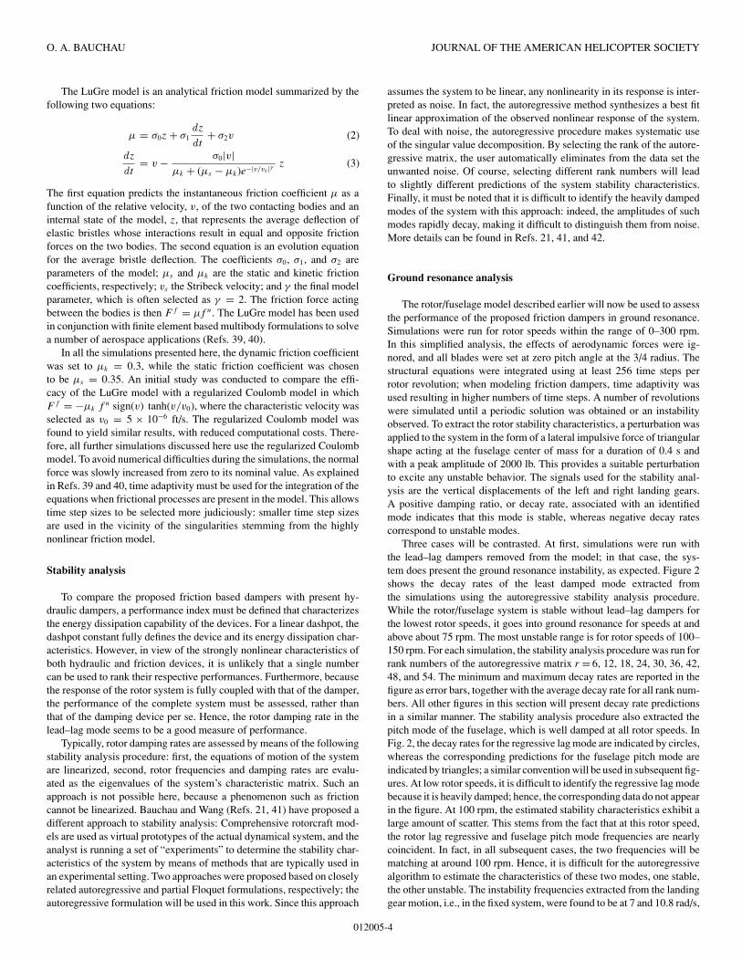
The first equation predicts the instantaneous friction coefficient μ as afunction of the relative velocity, v, of the two contacting bodies and aninternal state of the model, z, that represents the average deflection ofelastic bristles whose interactions result in equal and opposite frictionforces on the two bodies. The second equation is an evolution equationfor the average bristle deflection. The coefficients σ0, σ1, and σ2 areparameters of the model; μs and μk are the static and kinetic frictioncoefficients, respectively; vs the Stribeck velocity; and γ the final modelparameter, which is often selected as γ = 2. The friction force actingbetween the bodies is then F f = μf n. The LuGre model has been usedin conjunction with finite element based multibody formulations to solvea number of aerospace applications (Refs. 39, 40).

In all the simulations presented here, the dynamic friction coefficientwas set to μk = 0.3, while the static friction coefficient was chosento be μs = 0.35. An initial study was conducted to compare the effi-cacy of the LuGre model with a regularized Coulomb model in whichF f = −μk f n sign(v) tanh(v/v0), where the characteristic velocity wasselected as v0 = 5 × 10−6 ft/s. The regularized Coulomb model wasfound to yield similar results, with reduced computational costs. There-fore, all further simulations discussed here use the regularized Coulombmodel. To avoid numerical difficulties during the simulations, the normalforce was slowly increased from zero to its nominal value. As explainedin Refs. 39 and 40, time adaptivity must be used for the integration of theequations when frictional processes are present in the model. This allowstime step sizes to be selected more judiciously: smaller time step sizesare used in the vicinity of the singularities stemming from the highlynonlinear friction model.

Stability analysis

To compare the proposed friction based dampers with present hy-draulic dampers, a performance index must be defined that characterizesthe energy dissipation capability of the devices. For a linear dashpot, thedashpot constant fully defines the device and its energy dissipation char-acteristics. However, in view of the strongly nonlinear characteristics ofboth hydraulic and friction devices, it is unlikely that a single numbercan be used to rank their respective performances. Furthermore, becausethe response of the rotor system is fully coupled with that of the damper,the performance of the complete system must be assessed, rather thanthat of the damping device per se. Hence, the rotor damping rate in thelead–lag mode seems to be a good measure of performance.

Typically, rotor damping rates are assessed by means of the followingstability analysis procedure: first, the equations of motion of the systemare linearized, second, rotor frequencies and damping rates are evalu-ated as the eigenvalues of the system’s characteristic matrix. Such anapproach is not possible here, because a phenomenon such as frictioncannot be linearized. Bauchau and Wang (Refs. 21, 41) have proposed adifferent approach to stability analysis: Comprehensive rotorcraft mod-els are used as virtual prototypes of the actual dynamical system, and theanalyst is running a set of “experiments” to determine the stability char-acteristics of the system by means of methods that are typically used inan experimental setting. Two approaches were proposed based on closelyrelated autoregressive and partial Floquet formulations, respectively; theautoregressive formulation will be used in this work. Since this approach

assumes the system to be linear, any nonlinearity in its response is inter-preted as noise. In fact, the autoregressive method synthesizes a best fitlinear approximation of the observed nonlinear response of the system.To deal with noise, the autoregressive procedure makes systematic useof the singular value decomposition. By selecting the rank of the autore-gressive matrix, the user automatically eliminates from the data set theunwanted noise. Of course, selecting different rank numbers will leadto slightly different predictions of the system stability characteristics.Finally, it must be noted that it is difficult to identify the heavily dampedmodes of the system with this approach: indeed, the amplitudes of suchmodes rapidly decay, making it difficult to distinguish them from noise.More details can be found in Refs. 21, 41, and 42.

Ground resonance analysis

The rotor/fuselage model described earlier will now be used to assessthe performance of the proposed friction dampers in ground resonance.Simulations were run for rotor speeds within the range of 0–300 rpm.In this simplified analysis, the effects of aerodynamic forces were ig-nored, and all blades were set at zero pitch angle at the 3/4 radius. Thestructural equations were integrated using at least 256 time steps perrotor revolution; when modeling friction dampers, time adaptivity wasused resulting in higher numbers of time steps. A number of revolutionswere simulated until a periodic solution was obtained or an instabilityobserved. To extract the rotor stability characteristics, a perturbation wasapplied to the system in the form of a lateral impulsive force of triangularshape acting at the fuselage center of mass for a duration of 0.4 s andwith a peak amplitude of 2000 lb. This provides a suitable perturbationto excite any unstable behavior. The signals used for the stability anal-ysis are the vertical displacements of the left and right landing gears.A positive damping ratio, or decay rate, associated with an identifiedmode indicates that this mode is stable, whereas negative decay ratescorrespond to unstable modes.

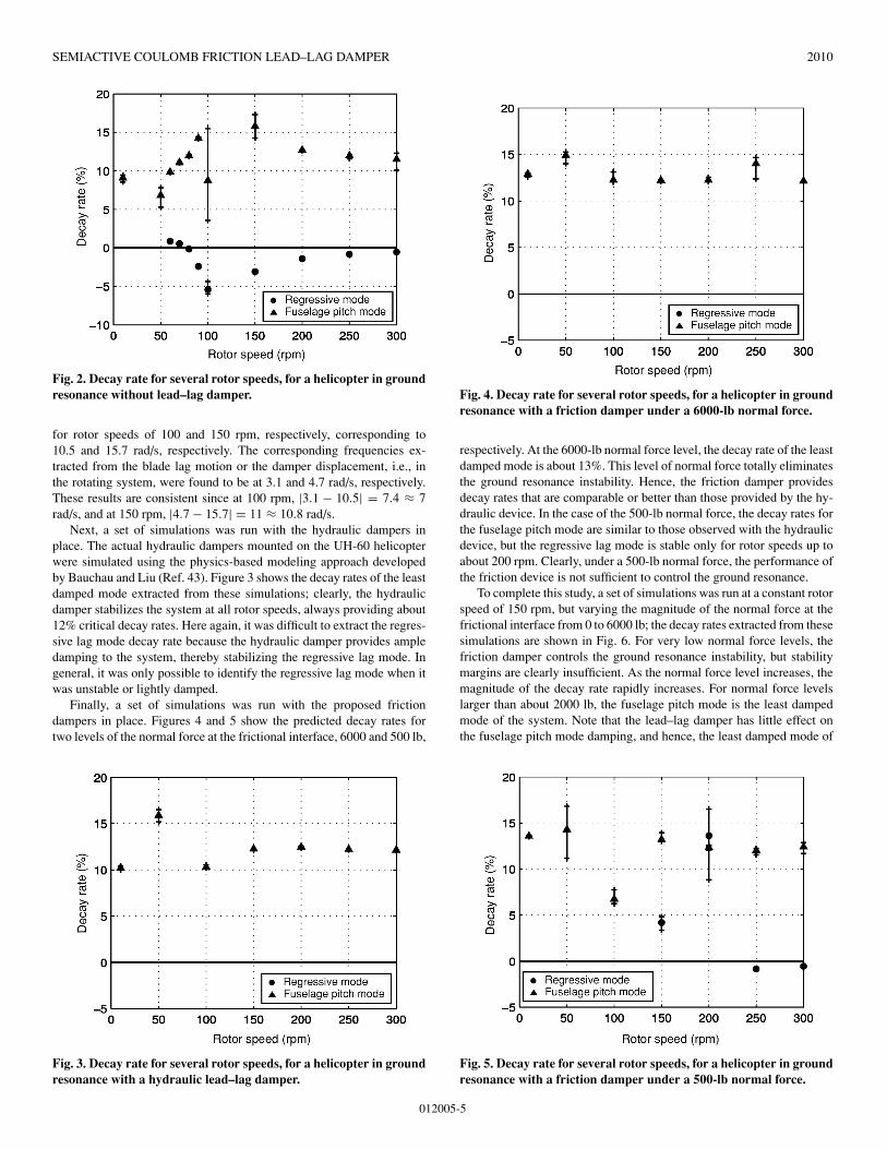
Three cases will be contrasted. At first, simulations were run withthe lead–lag dampers removed from the model; in that case, the sys-tem does present the ground resonance instability, as expected. Figure 2shows the decay rates of the least damped mode extracted fromthe simulations using the autoregressive stability analysis procedure.While the rotor/fuselage system is stable without lead–lag dampers forthe lowest rotor speeds, it goes into ground resonance for speeds at andabove about 75 rpm. The most unstable range is for rotor speeds of 100–150 rpm. For each simulation, the stability analysis procedure was run forrank numbers of the autoregressive matrix r = 6, 12, 18, 24, 30, 36, 42,48, and 54. The minimum and maximum decay rates are reported in thefigure as error bars, together with the average decay rate for all rank num-bers. All other figures in this section will present decay rate predictionsin a similar manner. The stability analysis procedure also extracted thepitch mode of the fuselage, which is well damped at all rotor speeds. InFig. 2, the decay rates for the regressive lag mode are indicated by circles,whereas the corresponding predictions for the fuselage pitch mode areindicated by triangles; a similar convention will be used in subsequent fig-ures. At low rotor speeds, it is difficult to identify the regressive lag modebecause it is heavily damped; hence, the corresponding data do not appearin the figure. At 100 rpm, the estimated stability characteristics exhibit alarge amount of scatter. This stems from the fact that at this rotor speed,the rotor lag regressive and fuselage pitch mode frequencies are nearlycoincident. In fact, in all subsequent cases, the two frequencies will bematching at around 100 rpm. Hence, it is difficult for the autoregressivealgorithm to estimate the characteristics of these two modes, one stable,the other unstable. The instability frequencies extracted from the landinggear motion, i.e., in the fixed system, were found to be at 7 and 10.8 rad/s,

012005-4


Fig. 2. Decay rate for several rotor speeds, for a helicopter in ground

resonance without lead–lag damper.

for rotor speeds of 100 and 150 rpm, respectively, corresponding to10.5 and 15.7 rad/s, respectively. The corresponding frequencies ex-tracted from the blade lag motion or the damper displacement, i.e., inthe rotating system, were found to be at 3.1 and 4.7 rad/s, respectively.These results are consistent since at 100 rpm, |3.1 − 10.5| = 7.4 ≈ 7rad/s, and at 150 rpm, |4.7 − 15.7| = 11 ≈ 10.8 rad/s.

Next, a set of simulations was run with the hydraulic dampers inplace. The actual hydraulic dampers mounted on the UH-60 helicopterwere simulated using the physics-based modeling approach developedby Bauchau and Liu (Ref. 43). Figure 3 shows the decay rates of the leastdamped mode extracted from these simulations; clearly, the hydraulicdamper stabilizes the system at all rotor speeds, always providing about12% critical decay rates. Here again, it was difficult to extract the regres-sive lag mode decay rate because the hydraulic damper provides ampledamping to the system, thereby stabilizing the regressive lag mode. Ingeneral, it was only possible to identify the regressive lag mode when itwas unstable or lightly damped.

Finally, a set of simulations was run with the proposed frictiondampers in place. Figures 4 and 5 show the predicted decay rates fortwo levels of the normal force at the frictional interface, 6000 and 500 lb,


resonance with a hydraulic lead–lag damper.


resonance with a friction damper under a 6000-lb normal force.

respectively. At the 6000-lb normal force level, the decay rate of the leastdamped mode is about 13%. This level of normal force totally eliminatesthe ground resonance instability. Hence, the friction damper providesdecay rates that are comparable or better than those provided by the hy-draulic device. In the case of the 500-lb normal force, the decay rates forthe fuselage pitch mode are similar to those observed with the hydraulicdevice, but the regressive lag mode is stable only for rotor speeds up toabout 200 rpm. Clearly, under a 500-lb normal force, the performance ofthe friction device is not sufficient to control the ground resonance.

To complete this study, a set of simulations was run at a constant rotorspeed of 150 rpm, but varying the magnitude of the normal force at thefrictional interface from 0 to 6000 lb; the decay rates extracted from thesesimulations are shown in Fig. 6. For very low normal force levels, thefriction damper controls the ground resonance instability, but stabilitymargins are clearly insufficient. As the normal force level increases, themagnitude of the decay rate rapidly increases. For normal force levelslarger than about 2000 lb, the fuselage pitch mode is the least dampedmode of the system. Note that the lead–lag damper has little effect onthe fuselage pitch mode damping, and hence, the least damped mode of


resonance with a friction damper under a 500-lb normal force.

012005-5


Fig. 6. Decay rate for several normal force levels, for a helicopter in

ground resonance with a rotor speed of 150 rpm.

the system, the fuselage pitch mode, retains a nearly constant decay ratefor all normal force levels greater than about 2000 lb.

Forward flight analysis

Next, the performance of the proposed friction damper will be as-sessed in the forward flight regime. The model described in the abovesections will be used here again, but the rotor hub is now connected toan inertial point; the rotor speed is set to its nominal speed of 258 rpmand the forward speed is 154.8 kt, corresponding to an advance ratio ofμ = 0.36. The aerodynamic model combines thin airfoil theory with athree-dimensional dynamic inflow model. The inflow velocities at eachspanwise location were computed using the finite state induced flowmodel developed by Peters et al. (Refs. 44, 45). The airfoil has a constantlift curve slope, a0 = 5.73, drag coefficient, cd = 0.018, and a vanish-ing moment coefficient about the quarter-chord. The number of inflowharmonics was selected as m = 10, corresponding to 66 aerodynamicinflow states for this problem.

Simulations were run with various normal load levels to assess theeffect of the normal force on the decay rate for the undesirable regressivelag mode. In each case, the stability analysis procedure was run for ranknumbers of the autoregressive matrix r = 12, 24, 36, 48, 60, 72, 84, 96,108, and 120. For each load level, the decay rates for these differentrank numbers were averaged and the minimal and maximal values werecomputed. Figure 7 shows that increasing the normal load level increasesthe regressive lag mode decay rate, as expected. Furthermore, in therange of normal loads investigated in this study, the relationship betweenthese two quantities seems roughly linear. As in the case of the groundresonance analysis, the damping capacity of the proposed friction devicecan exceed that of the currently installed hydraulic damper, for highenough levels of the normal force.

This finding is visually confirmed by observing Fig. 8, which showsthe response of the lead–lag angle to an initial excitation for the hydraulicand friction dampers with three different normal load levels: 2500, 5000,and 10,000 lb. It is clear that the hydraulic device provides higher levelsof damping than the friction device for normal force levels of 2500 and5000 lb, but at the 10,000-lb level, the situation is reversed. Clearly,the proposed friction device is able to provide damping on demand byvarying the normal force level. In forward flight at 154.8 kt, the rotor isstable without lead–lag dampers, although the decay rate is undesirably

Fig. 7. Evolution of the regressive decay rate with the normal load,

in forward flight at 154 kt. The horizontal line indicates the decay

rate obtained with the hydraulic damper.

0 1 2 3 42

4

6

8

10

0 1 2 3 42

4

6

8

10

0 1 2 3 42

4

6

8

10

Lag a

ngle

(deg)

0 1 2 3 42

4

6

8

10

Time (s)

Hydraulic

2500 lb

5000 lb

10,000 lb

Fig. 8. Time histories of the blade lag angle for several normal force

levels in forward flight at 154 kt.

012005-6


0 45 90 135 180 225 270 315 360−0.04

−0.03

−0.02

−0.01

0

Da

mp

er

stro

ke (

ft)

0 45 90 135 180 225 270 315 360−0.5

0

0.5

Da

mp

er

velo

city

(ft

/s)

0 45 90 135 180 225 270 315 360−4000

−2000

0

2000

4000

Da

mp

er

forc

e (

lb)

Azimuth (deg)

HydraulicFriction 5000 lb



Fig. 9. Comparison of the time histories of the damper stroke, the

damper velocity, and the damper force over one period in forward

flight at 154 kt.

low. With a semiactive device, the damping level in the various flightregimes can be selected independently; in forward flight, once a desireddamping level has been determined, Fig. 7 can be used to estimate therequired normal force level. For passive devices, the damping level is aconsequence of the physical characteristics of the damper, which havebeen selected to provide adequate energy dissipation characteristics inground resonance and maneuver flights.

As shown in Fig. 8, the asymptotic average lead–lag angles as wellas their waveforms are different for the hydraulic and friction damperswith various normal load levels. This underlines the fully coupled natureof the problem: Damper performance is not solely a consequence ofthe device’s physical characteristics but also of its interaction with thedynamical system. This is also observed in the top plot of Fig. 9, whichrepresents the damper stroke in the hydraulic damper and in the frictiondamper with a 5000-lb normal force, over one period of the rotor. Theother plots show the damper velocity and the damper force in both cases.It can be seen that the two responses share some similarities. In fact,comparing the force outputs of both dampers, it seems quite naturalthat the hydraulic damper has a slightly better decay rate than the frictiondamper under a 5000-lb normal force, although they are apparently close.Also note the square waves characteristics of friction behavior. It alsoshows that the peak damper forces are ±1500 lb in the friction damper,whereas those observed in the hydraulic damper are ±3200 lb. Clearly,the friction damper reduces blade inplane loads.

Assessment of the Concept of Selectivity

The preceding section has focused on adaptive damping or “dampingon demand.” With semiactive dampers, it is possible to proceed onestep further and selectively damp the component of damper stroke ata specific frequency, while minimally affecting other components. Tobe more precise, the stroking of a rotorcraft lead–lag damper consistsof the superposition of motions at the first lag frequency, ωζ , and theresponse at all other frequencies. The former contains motions due to thestable progressive mode, the collective and differential inplane modes,and the potentially unstable regressive inplane mode that is targeted here,whereas the latter contains, in particular, the contributions at 1P, and atnP in general. The relative velocity of the damper, v(t), is written asv(t) = vr (t) + vo(t), where vr is the relative velocity at the regressivelag frequency, whereas vo represents all other components. Included inthis latter category, is the large damper stroke rate at 1P, generated bythe Coriolis forces associated with the flapping of the blade; in forwardflight, this 1P component dominates the damper stroke rate. The reasonfor making a distinction between lag regressive and other componentsis clear: The purpose of the damper is to control the potentially unstableregressive lag mode. Passive dampers will generate damping forces thatdepend, in general, on the device’s stroke and stroke rate across the entirefrequency spectrum, and consequently, they apply large damping forcesin response to large 1P stroke rates. These large forces are not necessarysince the inherently stable 1P motion does not need damping, but yet, areapplied to the blade and hub, in turn creating large stresses and potentialfatigue problems. The concept of selective damping can now be definedmore precisely for rotorcraft problems: Can a semiactive damper be usedto selectively damp the regressive lag mode of the blade while minimallyaffecting the other modes?

Selective damping algorithm

To assess the concept of selectivity, a semiactive friction damper willbe considered. It is assumed that a controller adjusts the normal forceat the friction interface to be proportional to the relative velocity, i.e.,f n = (f n

ref/vref ) |v|, where f nref and vref are reference values of the normal

force and relative velocity, respectively. The friction force becomes F f =−crefv, where cref = μ(f n

ref/vref ). If the maximum normal force can bemodulated in time, the friction force becomes F f = −c(t)v, where 0 ≤c(t) ≤ cmax: the friction damper behaves like a viscous damper with anadjustable dashpot constant. Note that a similar effect could be obtainedwith magnetorheological dampers (Ref. 9), or with hydraulic dampersfeaturing controllable flow valves, although in both cases, some level ofnonlinearity would be typically observed. The present controller makesthe damper behave like a viscous damper, but other strategies are possible,such as a full normal force strategy (bang–bang controller). However,this strategy creates undesirable impulsive forces and simulations alsoshowed selective damping to be ineffective in this case. In view of theexploratory nature of this study, the simple model described above willbe used. Note that if the device is passive, i.e., c(t) = c, the damperbecomes a simple, linear viscous damper.

The work done by the damper force between two arbitrary times, tiand tf > ti , is

Wti→tf =∫ tf

ti

F f v d t = −∫ tf

ti

c(t)v2 d t ≤ 0 (4)

This work is necessarily negative, as expected in view of the dissipativenature of the device. Next, the work done by the damper force on theregressive lag component of the relative velocity during the same period

012005-7


is

Wti→tfr =

∫ tf

ti

F f vr d t = −∫ tf

ti

c(t)vvr d t ≤>

0 (5)

It is important to note that the instantaneous work done by the frictionforce on the regressive lag component can be negative, positive, or evenzero, because the product vvr can be negative, positive, or zero. Evena passive device, for which c(t) = c, could instantaneously add energyto the regressive lag mode, although the device is instantaneously dis-sipative, as implied by Eq. (4). This observation clearly underlines thefact that passive devices are not ideally suited to the targeted dampingof a specific component of the stroke rate. On the other hand, the sameobservation suggests a strategy for selective damping, when a semiactivedevice is available. If vvr > 0, the damper extracts energy from theregressive lag mode, whereas if vvr < 0, the damper adds energy tothe same mode. The following selective strategy is proposed: if vvr > 0,select c = cmax to maximize energy dissipation of the regressive lagmode, while possible, whereas if vvr < 0, select c = 0 to avoid addingany energy to the targeted mode. This approach will maximize energydissipation of the targeted mode.

Model problem

The concept of selectivity will be tested within the framework of theground resonance analysis developed by Coleman and Feingold (Ref. 20).Their model was modified to include the blades’ flapping motion in ad-dition to the lead–lag motion. The flapping degrees of freedom influencethe lead–lag degrees of freedom through the Coriolis coupling term.The presence of a flapping motion is representative of slope landing, forexample. The rotor consists of four identical rigid blades connected tothe hub by means of offset lag hinges. A semiactive friction damper islocated in each hinge. The hub is represented by a concentrated mass andis connected to the ground by springs and linear dashpots along two or-thogonal directions. All the model parameters can be found in Table 1. Tointroduce a 1P component into the lag motion, a sinusoidal flap motion ofthe blade was prescribed at the 1P frequency, βi = β0 +β1 sin ψi , whereβ0 = 15◦ and β1 = 7◦. Hence, the total lead–lag response containeda 1P contribution, a regressive component, and several other modes. Ahigh value of the coning angle β0 was chosen to ensure the presence of alarge enough 1P contribution, so as to better exhibit the identification andstabilization of the lag regressive component that might potentially besmall compared to the dominant (but stable) 1P component. The smallerthe amplitude of the 1P motion, the easier one would expect the identifi-cation of the lag regressive part to be; hence, a more demanding case isbeing considered here.

Using the multiblade coordinate transformation, the lead–lag angle,ζi , i = 1, 2, 3, 4, of each blade can be written as

ζi = ζ0 + ζs sin ψi + ζc cos ψi + (−1)i ζd (6)

where ζ0, ζs , ζc, and ζd are functions of the nondimensional time = t ,ψi is the azimuthal position of the ith blade, and the rotor angularspeed. It will be convenient to introduce the following notation for thecyclic component of the lead–lag angle, ζy,i = ζs sin ψi + ζc cos ψi , andthe nondimensional time derivative of the blade lead–lag angle becomes

ζ ∗i = ζ ∗

0 + ζ ∗y,i + (−1)i ζ ∗

d (7)

where the notation (·)∗ indicates a derivative with respect to the non-dimensional time .

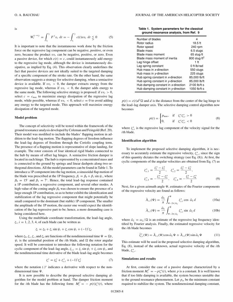
It is now possible to describe the proposed selective damping al-gorithm for the model problem at hand. The damper friction momentfor the ith blade has the following form: M

f

i = − p(t)ζ ∗i (t), where

Table 1. System parameters for the classicalground resonance analysis, from Ref. 9

Number of blades 4Rotor radius 18.5 ftRotor speed 240 rpmBlade mass 6.5 slugsBlade mass moment 65 slug·ftBlade mass moment of inertia 800 slug·ft2Lag hinge offset 1 ftLag spring constant 0 ft·lb/radHub mass in x-direction 550 slugsHub mass in y-direction 225 slugsHub spring constant in x-direction 85,000 lb/ftHub spring constant in y-direction 85,000 lb/ftHub damping constant in x-direction 2100 lb/ft·sHub damping constant in y-direction 1050 lb/ft·s

p(t) = c(t)d2 and d is the distance from the center of the lag hinge tothe lead–lag damper axis. The selective damping control algorithm nowbecomes

p(t) ={

pmax, if ζ ∗i ζ ∗

i,r > 0

0, if ζ ∗i ζ ∗

i,r < 0(8)

where ζ ∗i,r is the regressive lag component of the velocity signal for the

ith blade.

Identification algorithm

To implement the proposed selective damping algorithm, it is nec-essary to accurately estimate the regressive velocity, ζ ∗

i,r , since the signof this quantity dictates the switching strategy (see Eq. (8)). At first, thecyclic components of the angular velocities are obtained from Eq. (7) as

ζ ∗y,1 = ζ ∗

1 − ζ ∗3

2, ζ ∗

y,2 = ζ ∗2 − ζ ∗

4

2,

ζ ∗y,3 = − ζ ∗

1 − ζ ∗3

2, ζ ∗

y,4 = − ζ ∗2 − ζ ∗

4

2(9)

Next, for a given azimuth angle , estimates of the Fourier componentsof the regressive velocity are found as follows:

Ac,i() = ωζ

π

∫

−2π/ωζ

ζ ∗y,i cos ωζd (10a)

As,i() = ωζ

π

∫

−2π/ωζ

ζ ∗y,i sin ωζd (10b)

where ωζ = ωζ / is an estimate of the regressive lag frequency iden-tified by Fourier analysis. Finally, the estimated regressive velocity forthe ith blade becomes

ζ ∗i,r () = Ac,i() cos ωζ + As,i() sin ωζ (11)

This estimate will be used in the proposed selective damping algorithm,Eq. (8), instead of the unknown, actual regressive velocity of the ithblade, ζ ∗

i,r .

Simulations and results

At first, consider the case of a passive damper characterized by afriction moment M

f

i = −pζ ∗i (t), where p is a constant. It is well known

that if too little damping is available, the system becomes unstable dueto the ground resonance phenomenon. Let pcr be the minimum constantrequired to stabilize the system. The nondimensional damping constant,

012005-8


0 50 100 150 200−0.1

0

0.1q y

/R (

nondim

.)

0 50 100 150 200−0.05

0

0.05

q y/R

(nondim

.)

0 50 100 150 200−0.01

0

0.01

q y/R

(nondim

.)

0 50 100 150 200−0.01

0

0.01

ψ = Ωt (rad)

q y/R

(nondim

.)

SelectivePassive

SelectivePassive

SelectivePassive

SelectivePassive

Case a

Case b

Case c

Case d

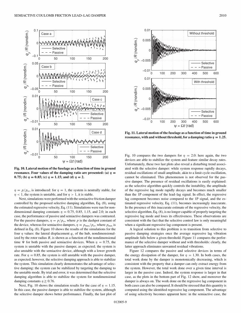
Fig. 10. Lateral motion of the fuselage as a function of time in ground

resonance. Four values of the damping ratio are presented: (a) η =0.75; (b) η = 0.85; (c) η = 1.15; and (d) η = 2.

η = p/pcr, is introduced: for η = 1, the system is neutrally stable, forη < 1, the system is unstable, and for η > 1, it is stable.

Next, simulations were performed with the semiactive friction dampercontrolled by the proposed selective damping algorithm, Eq. (8), usingthe estimated regressive velocity, Eq. (11). Simulations were run for non-dimensional damping constants η = 0.75, 0.85, 1.15, and 2.0; in eachcase, the performance of passive and semiactive dampers was contrasted.For the passive dampers, η = p/pcr, where p is the dashpot constant ofthe device, whereas for semiactive dampers, η = pmax/pcr, where pmax isdefined in Eq. (8). Figure 10 shows the results of the simulations for thefour η values: the lateral displacement qy of the hub, nondimensional-ized by the rotor radius R, is shown as a function of the nondimensionaltime for both passive and semiactive devices. When η = 0.75, thesystem is unstable with the passive damper, as expected; the system isalso unstable with the semiactive device, although with a lower growthrate. For η = 0.85, the system is still unstable with the passive damper,as expected; however, the selective damping approach is able to stabilizethe system. This simulation clearly demonstrates the advantage of selec-tive damping: the system can be stabilized by targeting the damping tothe unstable mode. By trial and error, it was determined that the selectivedamping algorithm is able to stabilize the system for nondimensionaldamping constants η >∼ 0.76.

Next, Fig. 10 shows the simulation results for the case of η = 1.15.In this case, the passive damper is able to stabilize the system, althoughthe selective damper shows better performance. Finally, the last plot of

0 100 200 300 400 500 600−0.01

−0.005

0

0.005

0.01

q y/R

(n

on

dim

.)

0 100 200 300 400 500 600−0.01

−0.005

0

0.005

0.01

ψ = Ωt (rad)

q y/ R

(n

on

dim

.)

SelectivePassive

SelectivePassive

Without threshold

With threshold


resonance, with and without threshold, for a damping ratio η = 1.25.

Fig. 10 compares the two dampers for η = 2.0: here again, the twodevices are able to stabilize the system and feature similar decay rates.Unfortunately, these two last plots also reveal a disturbing trend associ-ated with the selective damper: while system response rapidly decays,residual oscillations of small amplitude, akin to a limit cycle oscillation,cannot be eliminated. This phenomenon is not observed for the pas-sive damper. The presence of residual oscillations is easily explained:as the selective algorithm quickly controls the instability, the amplitudeof the regressive lag mode rapidly decays and becomes much smallerthan the 1P component of the lead–lag signal. In effect, the regressivelag component becomes noise compared to the 1P signal, and the es-timated regressive velocity, Eq. (11), becomes increasingly inaccurate.In the presence of this inaccurate estimate of the regressive velocity, theselective algorithm, Eq. (8), is no longer capable of properly targeting theregressive lag mode and loses its effectiveness. These observations areconsistent with the fact that the selective control law is only meaningfulwhen a significant regressive lag component is present.

A logical solution to this problem is to transition from selective topassive damping strategies once the average regressive lag vibrationamplitude falls below a given threshold. Figure 11 compares the perfor-mance of the selective damper without and with thresholds: clearly, thelatter approach eliminates unwanted residual vibrations.

Figure 12 compares the passive and selective devices in terms ofthe energy dissipation of the damper, for η = 1.30. In both cases, thetotal work done by the damper is monotonically decreasing, which isconsistent with the property that a damper can only extract energy fromthe system. However, the total work done over a given time interval islarger in the passive case. Indeed, the system response is larger in thatcase, as the plots in the bottom part of Fig. 12 show, and moreover thedamper is always on. The work done on the regressive lag component inboth cases can also be compared. It should be stressed that this quantity iscomputed using the identified regressive lag component. The advantageof using selectivity becomes apparent here: in the semiactive case, the

012005-9


0 10 20 30 40 50−0.03

−0.025

−0.02

−0.015

−0.01

−0.005

0

Work

done (

nondim

.)

0 10 20 30 40 50−0.03

−0.025

−0.02

−0.015

−0.01

−0.005

0

Work

done (

nondim

.)

0 10 20 30 40 50−0.01

−0.005

0

0.005

0.01

q y/R

(nondim

.)

0 10 20 30 40 50−0.01

−0.005

0

0.005

0.01

q y/R

(nondim

.)

0 10 20 30 40 50−10

−5

0

5

10

ψ = Ω t (rad)

ζ 1(d

eg)

0 10 20 30 40 50−15

−10

−5

0

5

10

ψ = Ω t (rad)

ζ 1 (

deg)

Total workWork on regressiveWork on other modes

Total workWork on regressiveWork on other modes

Fig. 12. Total work done by the damper, work done on the regressive component, and work done on the other components in ground resonance,

for η = 1.30. Passive case: left part; selective case: right part. See Fig. 13 for a more detailed view of the work done by the regressive lag

component.

work done on the regressive lag component decreases monotonically,whereas in the passive device, the instantaneous power on the regressivelag component can be positive, implying that energy is in fact transferredto the regressive lag component. Consequently, it can be observed thatthe work done on the regressive lag component over a given period oftime is larger in the selective case, leading to a better damping out of theinstability. This is clearly shown in Fig. 13, which represents the workdone on the regressive lag component in more detail.

Finally, simulations have been run that reveal some of the drawbacksto the use of selectivity: indeed, for the selective law to work correctly, theregressive lag component used in the control law needs to be properlyidentified. This is visually demonstrated in Fig. 14, which shows thelateral motion of the fuselage in the passive and selective cases, thelatter being this time performed with an error introduced intentionally inthe frequency identification: the identified regressive lag frequency usedin the control law was set to a value lower than that obtained throughFourier analysis by 2.5%, to simulate the unavoidable error inherent toany identification algorithm. It clearly shows that the passively stablesystem can be destabilized through an inappropriate control schedule.

In summary, it has been demonstrated that a simple algorithm forselective damping can be very effective. In fact, when using selectivity,it is possible to stabilize a system that would be unstable when using

Fig. 13. Work done on the regressive component in ground resonance.

012005-10



resonance. An erroneous value of the estimated regressive frequency

was used.

a passive damper of identical dashpot constant. On the other hand, se-lective damping also presents serious drawbacks. First, as the availabledamping of the device increases, the advantage of selectivity decreases.For fail safe design considerations, semiactive devices are likely to bebuilt with η > 1.0 to ensure system stability in the case of controlleror actuator failure. Hence, it is unlikely that selective damping will leadto dramatic performance improvements. Second, because the nonperi-odic regressive lag mode is targeted for damping, the selective damperactuation is itself nonperiodic; this will result in unwanted 1P fixed sys-tem vibrations. Third, the accurate identification of the regressive lagcomponent is indispensable. Finally, the actuation associated with selec-tive damping is more complex than that required for adaptive damping.Whereas adaptive damping calls for slow actuation, typically varyingwith flight condition only, selective damping requires a more complex,faster actuation schedule.

Conclusions

This paper has focused on the analysis and performance evaluationof semiactive, Coulomb friction lead–lag dampers. Both adaptive andselective damping strategies were investigated. Simulations were run inboth ground resonance and forward flight to assess the use of frictionas an energy dissipation mechanism to control the ground resonanceinstability and provide adequate lead–lag damping levels. The followingconclusions can be drawn from this study:

1) Through identification of modal decay rates, it was demonstratedthat the energy dissipation capacity of the proposed friction damperincreases with increasing normal force levels. Furthermore, the proposedconcept is able to match or exceed the damping levels of the presentlyinstalled hydraulic dampers on the UH-60 aircraft.

2) The ability to adapt the damping level of the proposed device en-ables the concept of damping on demand. For flight conditions requiringlower energy dissipation levels, it becomes possible to lower the damp-ing forces in the damper, as well as those applied to the blade and hub,resulting in lower stress levels and potential weight savings.

In the second part of this paper, the concept of selective damping wasinvestigated. Whereas many dampers are designed to absorb as muchenergy as possible, the purpose of rotorcraft lead–lag dampers is to con-trol the rotor regressive lag mode. The concept of selective dampingis to target energy dissipation to the regressive lag mode while min-

imally affecting the other modes. Selective algorithms were proposedand implemented within a simplified analytical framework. The follow-ing conclusions can be drawn from this exploratory study:

1) Selectivity does enhance the performance of lead–lag dampers. Infact, when using selectivity, it is possible to stabilize a system that wouldbe unstable when using a passive damper of identical dashpot constant.

2) While the potential of selective damping has been demonstrated,this concept faces numerous drawbacks that might prevent its practi-cal implementation. Indeed, selectivity requires increased actuation andcontroller complexity; furthermore, fail safe operation considerationsmight drive the design to a configuration where selectivity provides littleadvantage over less complex designs. Clearly, further studies would berequired to obtain fully satisfactory designs.

Acknowledgments

This work was sponsored under an SBIR contract with Materi-als Technologies Corporation, Monroe, CT. The contract monitor isDr. Thomas Maier.

References

1Gandhi, F., and Weller, W., “Active Aeromechanical Stability Aug-mentation Using Fuselage State Feedback,” American Helicopter Society42nd Annual Forum Proceedings, Virginia Beach, VA, April 29–May 1,1997.

2Gandhi, F., and Hathaway, E., “Optimized Aeroelastic Couplingsfor Alleviation of Helicopter Ground Resonance,” Journal of Aircraft,Vol. 35, (4), 1998, pp. 582–590.

3Gandhi, F., and Malovah, B., “Influence of Balanced RotorAnisotropy in the Design of Aeromechanically Stable Helicopters,” AIAAJournal, Vol, 37, (10), 1999, pp. 1152–1160.

4Gandhi, F., “Concepts for Damperless Aeromechanically StableRotors,” Proceedings of the Royal Aeronautical Society Innovation inRotorcraft Technology Conference, London, UK, June 25–26, 1997,pp. 14.1–14.31.

5Hathaway, E., and Gandhi, F., “Concurrent Optimization of Aero-elastic Couplings and Rotor Stiffness for the Alleviation of HelicopterAeromechanical Instability,” Journal of Aircraft, Vol. 38, (1), 2001,pp. 69–80.

6Hathaway, E., and Gandhi, F., “Individual Blade Control for Al-leviation of Helicopter Ground Resonance,” Proceedings of the 39thAIAA/ASME/ASCE/AHS/ASC Structures, Structural Dynamics, andMaterials Conference, Long Beach, CA, April 20–23, 1998, AIAA 98-2006, pp. 2507–2517.

7Marathe, S., Gandhi, F., and Wang, K. W., “Helicopter BladeResponse and Aeromechanical Stability with a Magnetorheological FluidBased Lag Damper,” Journal of Intelligent Material Systems and Struc-tures, Vol. 9, (4), 1998, pp. 272–282.

8Gandhi, F., Wang, K.W., and Xia, L., “Magnetorheological FluidDamper Feedback Linearization Control for Helicopter Rotor Applica-tion,” Smart Materials and Structures, Vol. 10, (1), 2001, pp. 96–103.

9Zhao, Y., Choi, Y. T., and Wereley, N. M., “Semiactive Dampingof Ground Resonance in Helicopters Using MagnetorheologicalDampers,” Journal of the American Helicopter Society, Vol. 49, (3), 2004,pp. 468–482.

10Hu, W., and Wereley, N. M., “Magnetorheological Fluid and Elas-tomeric Lag Damper for Helicopter Stability Augmentation,” Interna-tional Journal of Modern Physics B, Vol. 19, (7–9), 2005, pp. 1471–1477.

012005-11


11Yang, B. D., and Menq, C. H., “Characterization of Contact Kinemat-ics and Application to the Design of Wedge Dampers in TurbomachineryBlading, Part I: Stick-Slip Contact Kinematics,” ASME Journal ofEngineering for Gas Turbines and Power, Vol. 120, (3), 1999,pp. 410–417.

12Yang, B. D., and Menq, C. H., “Characterization of Contact Kinemat-ics and Application to the Design of Wedge Dampers in TurbomachineryBlading, Part II: Prediction of Forced Response and Experimental Ver-ification,” ASME Journal of Engineering for Gas Turbines and Power,Vol. 120, (3), 1999, pp. 418–423.

13Gaul, L., and Lenz, J, “Active Damping of Space Structures by Con-tact Pressure Control in Joints,” Mechanics of Structures and Machines,Vol. 26, (1), 1998, pp. 81–100.

14Gaul, L., and Nitsche, R., “Friction Control for Vibration Suppres-sion,” Mechanical Systems and Signal Processing, Vol. 14, (2), 2000,pp. 139–150.

15Gaul, L., and Nitsche, R., “The Role of Friction in MechanicalJoints,” Applied Mechanics Reviews, Vol. 54, (2), 2001, pp. 93–105.

16Gaul, L., Albrecht, H., and Wirnitzer, J., “Semiactive Damping ofLarge Space Truss Structures Using Friction Joints,” Proceedings of theSPIE—The International Society for Optical Engineering, Vol. 4935,2002, pp. 232–243.

17Gaul, L., Albrecht, H., and Wirnitzer, J., “Semiactive Friction Damp-ing of Large Space Truss Structures,” Shock and Vibration, Vol. 11, (4),2004, pp. 173–186.

18Ferri, A. A., and Heck, B. S., “Analytical Investigation of DampingEnhancement Using Active and Passive Structural Joints,” Journal ofGuidance, Control, and Dynamics, Vol. 15, (1), 1992, pp. 1258–1264.

19Dupont, P., Kasturi, P., and Stokes, A., “Semiactive Control of Fric-tion Dampers,” Journal of Sound and Vibration, Vol. 202, (2), 1997,pp. 203–218.

20Coleman, R. P., and Feingold, A. M., “Theory of Self-Excited Me-chanical Oscillations of Helicopter Rotors with Hinged Blades,” NACATechnical Report 1351, 1956.

21Bauchau, O. A., and Wang, J. L., “Efficient and Robust Approachesto the Stability Analysis of Large Multibody Systems,” Journal ofComputational and Nonlinear Dynamics, Vol. 3, (1), January 2008,pp. 011001 1–12.

22Bousman, W. G., and Maier, T., “An Investigation of HelicopterRotor Blade Flap Vibratory Loads,” American Helicopter Society 48thAnnual Forum Proceedings, Washington, DC, June 3–5, 1992.

23Bauchau, O. A., Bottasso, C. L., and Nikishkov, Y. G., “ModelingRotorcraft Dynamics with Finite Element Multibody Procedures,” Math-ematical and Computer Modeling, Vol. 33, (10–11), 2001, pp. 1113–1137.

24Welsh, W. A., “Simulation and Correlation of a Helicopter Air-OilStrut Dynamic Response,” American Helicopter Society 43rd AnnualForum Proceedings, St. Louis, MO, May 18–20, 1987.

25Welsh, W. A., “Dynamic Modeling of a Helicopter Lubrication Sys-tem,” American Helicopter Society 44th Annual Forum Proceedings,Washington, DC, June 16–18, 1988.

26Oden, J. C., and Martins, J. A. C., “Models and Computational Meth-ods for Dynamic Friction Phenomena,” Computer Methods in AppliedMechanics and Engineering, Vol. 52, (2), 1985, pp. 527–634.

27Shigley, J. E., and Mischke, C. R., Mechanical Engineering Design,McGraw-Hill Book Company, New York, 1989, Chapter 6.

28Cardona, A., and Geradin, M., “Kinematic and Dynamic Analysisof Mechanisms with Cams,” Computer Methods in Applied Mechanicsand Engineering, Vol. 103, (1), 1993, pp. 115–134.

29Banerjee, A. K., and Kane, T. R., “Modeling and Simulation of RotorBearing Friction,” Journal of Guidance, Control, and Dynamics, Vol. 17,1994, pp. 1137–1151.

30Bauchau, O. A., “On the Modeling of Friction and Rolling in FlexibleMulti-Body Systems,” Multibody System Dynamics, Vol. 3, (1), 1999,pp. 209–239.

31Bauchau, O. A., and Rodriguez, J., “Modeling of Joints with Clear-ance in Flexible Multibody Systems,” International Journal of Solidsand Structures, Vol. 39, (1) 2002, pp. 41–63.

32Valanis, K. C., “A Theory of Viscoplasticity without a Yield Surface,”Archives of Mechanics, Vol. 23, (4), 1971, pp. 171–191.

33Hsu, T-K., and Peters, D. A., “A Simple Dynamic Model for Sim-ulating Draft-Gear Behavior in Rail-Car Impacts,” ASME Journal ofEngineering for Industry, Vol. 100, (2), November 1978, pp. 492–496.

34Dahl, P. R., “Solid Friction Damping of Mechanical Vibrations,”AIAA Journal, Vol. 14, (6), 1976, pp. 1675–1682.

35Haessig, D. A., and Friedland, B., “On the Modeling and Simula-tion of Friction,” ASME Journal of Dynamic Systems, Measurement andControl, Vol. 113, (1), 1991, pp. 354–362.

36Canudas de Wit, C., Olsson, H., Astrom, K. J., and Lischinsky, P., “ANew Model for Control of Systems with Friction,” IEEE Transactionson Automatic Control, Vol. 40, (2), 1995, pp. 419–425.

37Swevers, J., Al-Bender, F., Ganesman, C. G., and Prajogo, T., “AnIntegrated Friction Model Structure with Improved Presliding Behaviorfor Accurate Friction Compensation,” IEEE Transactions on AutomaticControl, Vol. 45, (4), 2000, pp. 675–686.

38Lampaert, V., Swevers, J., and Al-Bender, F., “Modification of theLuuven Integrated Friction Model Structure,” IEEE Transactions onAutomatic Control, Vol. 47, (4), 2002, pp. 683–687.

39Bauchau, O. A., Rodriguez, J., and Bottasso, C. L., “Modeling ofUnilateral Contact Conditions with Application to Aerospace SystemsInvolving Backlash, Freeplay and Friction,” Mechanics Research Com-munications, Vol. 28, (5), 2001, pp. 571–599.

40Bauchau, O. A., and Ju, C. K., “Modeling Friction Phenomenain Flexible Multibody Dynamics,” Computer Methods in Applied Me-chanics and Engineering, Vol. 195, (50–51), October 2006, pp. 6909–6924.

41Bauchau, O. A., and Wang, J. L., “Stability Analysis of ComplexMultibody Systems,” Journal of Computational and Nonlinear Dynam-ics, Vol. 1, (1), January 2006, pp. 71–80.

42Bauchau, O. A., and Wang, J. L., “Stability Evaluation and Sys-tem Identification of Flexible Multibody Systems,” Multibody SystemDynamics, Vol. 18, (1), October 2007, pp. 95–106.

43Bauchau, O. A., and Liu, H., “On the Modeling of Hydraulic Com-ponents in Rotorcraft Systems,” Journal of the American HelicopterSociety, Vol. 51, (2), April 2006, pp. 175–184.

44Peters, D. A., Karunamoorthy, S., and Cao, W. M., “Finite StateInduced Flow Models, Part I: Two-Dimensional Thin Airfoil,” Journalof Aircraft, Vol. 32, (2), 1995, pp. 313–322.

45Peters, D. A., and He, C. J., “Finite State Induced Flow Models,Part II: Three-Dimensional Rotor Disk,” Journal of Aircraft, Vol. 32, (2),1995, pp. 323–333.

012005-12

semiactive coulomb friction lead–lag dampers€¦ · dissipation characteristics of the device...

Documents