Senate Bill 350 Study Volume VIII: Economic Impact Analysis PREPARED FOR

PREPARED BY

David Roland-Holst

Drew Behnke

Samuel Evans

Cecilia Han Springer

Sam Heft-Neal

July 8, 2016

Senate Bill 350 Study The Impacts of a Regional ISO-Operated Power Market on California

List of Report Volumes

Executive Summary

Volume I. Purpose, Approach, and Findings of the SB 350 Regional Market Study

Volume II. The Stakeholder Process

Volume III. Description of Scenarios and Sensitivities

Volume IV. Renewable Energy Portfolio Analysis

Volume V. Production Cost Analysis

Volume VI. Load Diversity Analysis

Volume VII. Ratepayer Impact Analysis

Volume VIII. Economic Impact Analysis

Volume IX. Environmental Study

Volume X. Disadvantaged Community Impact Analysis

Volume XI. Renewable Integration and Reliability Impacts

Volume XII. Review of Existing Regional Market Impact Studies

Volume VIII. SB 350 Study: Economic Model & Impacts Final Report

Prepared for:

Berkeley Economic Advising and Research 1442A Walnut Street, Suite 108 Berkeley, CA 94705 www.bearecon.com July 8, 2016 © All rights reserved.

Final Report

-VIII-2-

Executive Summary California’s Senate Bill No. 350—the Clean Energy and Pollution Reduction Act of 2015—(SB 350) requires the California Independent System Operator (CAISO, Existing ISO, or ISO) to conduct one or more studies of the impacts of a regional market enabled by governance modifications that would transform the ISO into a multistate or regional entity (Regional ISO). SB 350, in part, specifically requires an evaluation of how regionalization would impact the creation or retention of jobs and other benefits to the California economy. Understanding these economic impacts is an integral part of the policy making process, and as a result Berkeley Economic Advising and Research (BEAR) has been engaged to model these impacts. This report is Volume VIII of XII of an overall study in response to SB 350’s legislative requirements. The BEAR dynamic economic forecasting model was used to evaluate California’s long-term growth prospects from developing a Regional ISO. Results are generated for 3 primary scenarios and 1 sensitivity scenario across 3 time periods. Current Practice (CP) refers to business as usual renewables procurement to meet California’s 50% Renewable Portfolio Standard by 2030 (50% RPS), the CAISO footprint as-is, and a 2,000 MW limit on net bilateral sales from CAISO entities. Two regionalization scenarios were compared to Current Practice. Regional 2 examines a regional market with business as usual renewables procurement and a regional ISO that includes most of U.S. WECC. Regional 3 examines a regional market with more out-of-state renewables procurement and a regional ISO that includes most of U.S. WECC. The study considers a sensitivity to the Current Practice scenario where the limit on net bilateral sales from CAISO entities is increased to 8,000 MW. As an initial baseline we provide evidence-based support that California’s higher Renewable Portfolio Standard (“RPS”) (50% by 2030) will provide a wide range of benefits to California households and enterprises. Across all scenarios, including the Current Practice scenario, we project higher statewide gross product, real output, state revenue, and employment. By 2030, we estimate there will be an additional 90,000 – 110,000 statewide jobs created from the 50% RPS policy goal depending on scenario analyzed. Furthermore, we find that reduced energy rates will lead to increase household income across every scenario, ensuring that an increased RPS will provide a stream of benefits to all Californians. While these findings offer support that a clean energy future is beneficial to the California economy, there are important differences between the scenarios that are worth noting. Most notably, we find that regionalization (scenarios Regional 2 and Regional 3) offers the most benefits to California in terms of job creation and income gains. Specifically, we find that regionalization can create 9,900 (Regional 3) to 19,300 (Regional 2) more jobs than the Current Practice scenario in 2030. Furthermore, the more affordable energy from regionalization offers further stimulus for the state economy, creating jobs that increase community real incomes by the equivalent of $290 (Regional 2) to $550 (Regional 3) per household in 2030.

Final Report

-VIII-3-

Although there will be less jobs from renewable buildout created in the regionalization scenarios due to the lower renewable capacity investments within California, we find that efficiency gains and the associated ratepayer savings will spur induced jobs through increased spending on services and consumption. Consequently, the net employment impacts from regionalization are positive. This finding is significant as these jobs are often “invisible” in the sense they are not directly captured or advocated for by the renewable buildout. However, these jobs are equally as important, and arguably more so, as they allow increased discretionary spending among lower socio-economic groups, and spur job creation across the entire state. Indeed, we find that hundreds of disadvantaged communities stand to receive significant job creation and income gains. As these communities are the most at-risk and underrepresented, our findings demonstrate that a regional renewable energy market will benefit all of California. The results for disadvantaged communities are discussed in Volume X of the SB 350 study.

Final Report

-VIII-4-

Table of Contents

I. Introduction ............................................................................................................................. VIII-5

II. Previous Literature ............................................................................................................... VIII-5 A. Estimating Impacts ........................................................................................................................ VIII-5 B. Previous Studies ............................................................................................................................. VIII-6

III. Model and Methodology ....................................................................................................... VIII-8 A. BEAR Model Description .............................................................................................................. VIII-8 B. Scenarios ......................................................................................................................................... VIII-10 C. Disaggregation .............................................................................................................................. VIII-10

1. Step 1 – Census Tracts ........................................................................................................................... VIII-11 2. Step 2 – Disadvantaged Community Level .................................................................................... VIII-12

IV. Results ..................................................................................................................................... VIII-12 A. Baseline Effects of Investment in 50% RPS ........................................................................ VIII-12 B. Impact of Regionalization ......................................................................................................... VIII-13

1. Employment Impacts by Occupation .............................................................................................. VIII-14 2. Impacts by Income Decile .................................................................................................................... VIII-18 3. Sensitivity Analysis ................................................................................................................................. VIII-20

V. Conclusion ............................................................................................................................. VIII-20

VI. References ............................................................................................................................. VIII-21

Final Report

-VIII-5-

I. Introduction Comparing scenarios, we find that a regional energy market in 2030 (Regional 2 and Regional 3) can create 9,900 – 19,400 more jobs than the Current Practice (CP 1), primarily through making electricity more affordable and the associated induced job effects from these savings. Specifically, the increased affordable energy from regionalization is expected to produce a higher statewide household real disposable income of $300 - $550 per household in 2030. Although Current Practice will see the most jobs directly linked to the large in-state renewable buildout requirements from 33% to 50%, a regional market in California can help the state balance both ratepayer savings and renewable buildout job creation. Indeed, we find that the regional market with California-focused procurement (Regional 2) offers the highest impact on statewide output and employment compared to Current Practice 1 and Regional 31. The balance of this section of the SB350 report is organized as follows: Sections 2 and 3 provide background information and details the methodological approach used for this analysis; Section 4 presents our main findings of state-wide impacts across scenarios2; and Section 5 provides conclusions.

II. Previous Literature

A. Estimating Impacts As explained in E3’s report (Volume IV), regionalization could have a significant impact on the location and characteristics of new renewable generation resources developed by California to meet its 50% Renewable Portfolio Standard (“RPS”) by 2030. Investments of this magnitude will have a material effect on the state’s economy. However, estimating the economic impacts of the different investment scenarios is complicated as there are several economic drivers of income and job dynamics. In general, these drivers can be classified under one of three groups:

1. Power Capacity Investment – These are the economic impacts associated with the direct build out of new renewable generation. This includes both direct jobs working on the construction of the facility and operations, as well as indirect supply chain related jobs. There are also induced effects through increased household income from related jobs supporting the renewable generation buildout(?).

2. Infrastructure Investment – Increased renewable buildout also requires a related investment in infrastructure, such as new or upgraded transmission, to ensure the

1 As discussed later in the section, a Current Practice sensitivity case (Scenario 1B) that assumes high bilateral exports absent a regional market produced the greatest employment impact but is very unlikely to materialize in practice due to the challenges of exporting large amounts of renewables under the current market structure. 2 More details on disadvantaged community effects are also presented in Volume 10.

Final Report

-VIII-6-

new generation reliably connects to the grid. This associated increase in infrastructure produces a variety of direct, indirect, and induced jobs.

3. Income/expenditure effects of electricity rate reductions – The implementation of the 50% RPS will affect electricity rates, resulting in a change in discretionary income. The associated expenditure effects of this change will impacts jobs across the entire economy through different spending patterns.

Adding further complexity to the estimation challenge is the fact that the income and job growth across all of these drivers will occur through a combination of effects:

1. Direct Effects – This is the increased economic activity in response to direct spending (either investment or consumption) on capacity buildout (e.g. jobs associated with the direct renewable buildout such as construction or operations).

2. Indirect Effects – This is the economic activity in enterprises linked by supply chains to directly affected sectors (e.g. suppliers of input components and raw materials)

3. Induced Effects – Demand from rising household income (e.g. spending by employed of directly and indirectly affected firms or from ratepayer savings).

Of particular interest are the induced effects as they are often the largest driver of job creation, but can be challenging to quantify. As a result, a model that does not accurately reflect these subtleties nor captures the entire supply chain of California will produce biased results.

B. Previous Studies There have been a few previous studies that consider how renewable energy contributes to job creation in California. The majority of these studies are based on voluntary survey results and offer past assessments of existing projects within the state. The California Advanced Energy Employment Survey is a publication-based on a survey of more than 2,000 companies in California. The survey reports some 431,800 jobs in the advanced energy economy in 2014. However, the majority of jobs (70%) are captured in the energy efficiency sector. If we strictly consider the advanced electricity generation sector, the report finds 95,000 employed in this sector, with the majority working in solar generation (~73,000). The report makes no distinction between those who work in utility-scale solar versus rooftop solar. Utility-scale wind generation was estimated to employ an additional 3,270 workers. Two recent reports from the Donald Vial Center on Employment in the Green Economy (which is affiliated with the Berkeley Labor Center) have studied how renewable energy contributes to job growth. The first, “Environmental and Economic Benefits of Building Solar in California,” by Peter Philips (2014) considers the employment effects of building 4,250 MW of utility-scale solar powered facilities over the previous five years. This report offers a useful comparison to this SB350 report as it focuses on utility-scale solar and relies on actual industry data.

Final Report

-VIII-7-

Phillips (2014) finds that an estimated 10,200 construction job-years3 were created during the rapid expansion of utility-scale solar generation facilities from 2010–2014. On average, these jobs paid $78,000 per year and offered health and pension benefits. Additionally, 136 permanent operations and maintenance job-years were created and are expected to last the lifetime of these facilities paying $69,000 a year on average with benefits. There were also an estimated 1,600 job-years created in the supply chain to perform other new business activities associated with construction. Finally, the newly-created jobs boosted consumer spending, resulting in an additional 3,700 jobs-years to meet the increased consumer demand. In total, this suggests an estimated 15,000 job-years were created from some 1,350 MW of increased solar generation capacity constructed in the timeframe of 2010–2014. The Philips (2014) study methodology is largely based on a review of existing literature. First, he identifies the electricity generation capacity of new utility-scale solar projects that were built or under construction between 2010 and 2014. Next, using four other studies, Philips takes the average number of job-years, supply chain multipliers, income, and pension benefits per MW installed from three large PV projects in central and southern California.4 He then multiplies the total number of estimated MW by the number of job-years (or other variable) per MW to obtain the estimates given above. The second report from the Donald Vial Center is, “Job Impacts of California’s Existing and Proposed Renewables Portfolio Standard,” by Betony Jones, Peter Philips, and Carol Zabin (2015). This study considers both the historical job creation for California’s renewable energy investments between 2003 and 2014 and forecasts estimates for jobs from 2015 to 2030 to meet the 50% RPS. Their study includes other sources of renewables outside of solar (such as wind), but does not include jobs created from renewable self-generation, which does not count towards the 50% RPS directly. They also do not report on jobs in operations and maintenance of these new plants as the authors argue that they are much smaller in quantity, and are unlikely to change significantly from the transition from conventional to renewable sources. Finally, the authors do not consider the jobs required for new transmission infrastructure or increased energy storage, both of which are likely needed to achieve the 50% RPS goal. Jones et al. consider both the historical creation of jobs in the timeframe 2003 – 2014 as well as forecasting jobs creation in 2015 – 2030. Much like Philips (2014), the authors’ first start with the total amount of renewable energy capacity that was built between 2003 and 2014, as well as estimates needed to achieve 50% RPS by 2030. The authors find that from 3 Jobs here mean job-years, or 2,080 hours of work. Construction workers are often rotated off jobs to get experience in other types of construction over the course of a year, and therefore one job year may be spread across two or more workers. In contrast, the study’s estimated 136 operations and maintenance jobs each represent 25 job-years, with each job lasting the expected lifetime of a newly-built solar electrical generation facility. 4The reports are: Stephen F. Hamilton, Darin Smith and Tepa Banda, “Economic Impact to San Luis Obispo County of the California Valley Solar Ranch,” Appendix 14B, December, 2010; Stephen F. Hamilton, Mark Berkman and Michelle Tran, “Economic and Fiscal Impacts of the Topaz Solar Farm,” March, 2011; Aspen Group, “Socioeconomic and Fiscal Impacts of the California Valley Solar Ranch and Topaz Solar Farm Projects on San Luis Obispo County,” January, 2011. Mark Berkman and Wesley Ahlgren, “Economic and Fiscal Impacts of the Desert Sunlight Solar Farm,” The Brattle Group (private communication with the author).

Final Report

-VIII-8-

2003 – 2014, California added some 7,000 MW of in-state capacity and is projected to need an additional 30,600 – 37,400 MW of additional capacity to meet the 50% RPS. The authors use the JEDI model to then provide a historical estimate of the number of jobs created and forecast future jobs. They find that in 2003 – 2014 about 52,000 direct job-years were created due to the construction of renewable energy plants. This includes both labor-based jobs and professional services. Including both the related indirect jobs (from inputs) and induced jobs (from increased consumer spending in the service sector) this estimate stretches to 130,000 total job-years. Note that these estimates are gross, rather than net. For the period from 2015 – 2030, the authors find that increasing the RPS to 50% by 2030 would create an additional 354,000 (low scenario) to 429,000 (high scenario) direct construction job-years. Including both indirect and induced jobs, this number becomes an estimated 879,000 to 1,067,000 job-years by 2030. In terms of permanent jobs instead of job years, these numbers represent some 23,600 to 28,600 direct full-time construction jobs and about 58,600 to 71,100 total full-time jobs from 2015 – 2030. It should be noted that these numbers represent “cumulative jobs” across the 2015 – 2030 period, a somewhat ambiguous aggregation of differences form reference employment levels over 15 years. In more concrete terms, annual average job creation and the increase in the standing labor force by 2030 are less than 10% of these cumulative numbers. The authors concede that their estimates likely overstate the amount of jobs created. They compare their results to their co-author Philips’ study from 2014 and find that JEDI overestimates direct jobs per MW, especially for solar which Philips (2014) has industry data for. For example, Philips (2014) estimates approximately 2.4 direct jobs per MW, while Jones et al. (2015) estimate 5.8 direct jobs per MW. Therefore, they conclude that the JEDI model is best used for comparisons between alternative scenarios and technology mixes than for absolute job numbers.

III. Model and Methodology

A. BEAR Model Description

The BEAR model is a dynamic economic forecasting model for evaluating long-term growth prospects for California (Roland-Holst, 2015). The model is an advanced policy simulation tool that models demand, supply, and resource allocation across the California economy, estimating economic outcomes annually over the period 2015–2030. This kind of Computable General Equilibrium (“CGE”) model is a state-of-the-art economic forecasting tool, using a system of equations and detailed economic data that simulate price-directed interactions between firms and households in commodity and factor markets. The role of government, capital markets, and other trading partners are also included, with varying degrees of detail, to close the model and account for economy-wide resource allocation, production, and income determination.

Final Report

-VIII-9-

BEAR is calibrated to a 2013 dataset of the California economy and it includes highly disaggregated representation of firm, household, employment, government, and trade behavior (Table 1). The model’s 2015 - 2030 baseline is calibrated to the California Department of Finance economic and demographic projections. The model’s baseline is recalibrated to incorporate the new data whenever new projections are released.

Table 1: BEAR 2013 - Current Structure

1. 195 production activities

2. 195 commodities (includes trade and transport margins)

3. 15 factors of production

4. 22 labor categories

5. Capital

6. Land

7. Natural capital

8. 10 Household types, defined by income decile

9. Enterprises

10. Federal Government (7 fiscal accounts)

11. State Government (27 fiscal accounts)

12. Local Government (11 fiscal accounts)

13. Consolidated capital account

14. External Trade Account

For the SB 350 study the BEAR model was aggregated to 60 economic sectors (Table 2). The electric power sector was disaggregated by 8 generation types in order to be consistent with the portfolios generated by the RESOLVE and PSO models.

Final Report

-VIII-10-

Table 2: 60 Sector BEAR Model Aggregation

B. Scenarios

The BEAR model produces results at the state level. Results are generated for 3 primary scenarios and 1 sensitivity scenario across 3 time periods. The scenarios are:

• Current Practice 1: Current Practice Procurement, CAISO operations, 2,000MW export limit

• Regional 2: Current Practice Procurement, WECC-wide operations, 8,000 MW export limit

• Regional 3: WECC-wide Procurement, WECC-wide operations, 8,000 MW export limit

• Sensitivity 1b: Current Practice Procurement, CAISO operations, 8,000MW export limit

The reporting years for the economic study are: 2020, 2025, and 2030.

C. Disaggregation

The process of estimating economic impacts on disadvantaged communities is carried out in several steps. This assessment technique leverages available data to downscale state level estimates to the census tract level conforming to disadvantaged community definitions. Detailed descriptions of each step are presented below.

Final Report

-VIII-11-

Figure 1: Downscaling Results to Identify Impacts of Disadvantaged Communities

1. Step 1 – Census Tracts

State-wide results produced by the BEAR model are first disaggregated to individual census tracts. Complete data on economic activities are not available at the census tract level, so it is not possible to build Social Accounting Matrices (SAMs) for individual census tracts. Instead, we construct census tract shares of state level economic activity for select variables of interest, i.e. income by decile, sector of employment, and occupation. Census tract estimates of these values are derived from the American Communities Survey (“ACS”)5 using the 5-year averages covering the period 2008-2013.

Income

The ACS reports income by tax bracket, however, the BEAR model estimates impacts on income by decile. Consequently, tax brackets were converted to income decile according to the share of overlap in each category. The number of households in each income decile was calculated for each census tract. State level income estimates were then shared out across census tracts according to the number of households in each income decile in each census tract.

The income estimates are presented as community income per household in 2030. In order to estimate the number of households in each census tract in 2030 we use Department of Finance estimates of population growth by county. We assume that population growth within counties is constant across census tracts and that household size remains constant so population growth is equivalent to growth in households. Relying on these assumptions, we calculate household growth rates for each census tract and apply them to the current number of households in order to forecast the number of households in each census tract in 2030.

5 http://factfinder.census.gov/

Final Report

-VIII-12-

Jobs

Job estimates from the BEAR model measure total jobs by occupation. Jobs due to ratepayer impacts at the state level are calculated by netting out statewide total estimated direct jobs. Jobs by occupation resulting from ratepayer savings are then downscaled from state to census tract level according to the number of employees in each occupation in each census tract. Direct jobs are downscaled from the county to census tract level according to the number of employees in construction-based occupations in each census tract. Renewable buildout and ratepayer savings jobs are then summed to estimate total jobs in each census tract.

2. Step 2 – Disadvantaged Community Level

In the final step, we use CalEnviroScreen 2.0 (“CES”)6 to identify census tracts designated as disadvantaged communities. We define disadvantaged communities as census tracts in the top 25th percentile of CES scores. By this definition, there are 2,009 disadvantaged communities (census tracts) in California. Income and job estimates for the subset of census tracts meeting this condition are presented in Volume X of the SB 350 study.

IV. Results Study results are presented below in two formats. Section 4.1 presents results comparing all scenarios to a hypothetical reference point that maintains the state’s current 33% RPS. Section 4.2 fulfills the direct requirements of SB350 by isolating the specific impacts of regionalization.

A. Baseline Effects of Investment in 50% RPS To better understand how California’s future renewables investments could affect the state’s economy and job creation we simulated a hypothetical reference point in which the state maintains its 33% RPS and does not expand to 50% by 2030. By first doing this we find strong evidence that regional electric power trading can benefit the California economy across a variety of indicators. Table 3 shows the percentage change from the reference scenario in 2030 for gross state product, real output, employment, state revenue, and real wage. The differences reported are estimated with respect to a reference scenario assuming no additional RPS investment from 2020. For Current Practice 1, we find increases ranging from 0.21% (state revenue) to 0.48% (real income).

6 http://oehha.ca.gov/ej/pdf/CES2_0SHP.zip

Final Report

-VIII-13-

Table 3: Baseline Impacts of Moving from 33% RPS to 50% RPS (Percent Change

from Reference in 2030)

Current Practice 1 Regional 2 Regional 3

Gross State Product 0.32% 0.37% 0.35%

Real Output 0.35% 0.40% 0.39%

Employment 0.29% 0.35% 0.32%

Real Income 0.48% 0.53% 0.61%

State Revenue 0.21% 0.33% 0.34%

Percent changes are useful in comparing the relative impacts between different scenarios, but do not give a clear idea to the size of these effects. To counter this, we also report our findings in terms of raw number in Table 4. These results illustrate the size of the impacts with Gross State Product increasing some $11.3 – $13 billion depending on the scenario. Real income is projected to increase the largest, ranging between $26.9 billion - $34.7 billion depending on scenario. In regards to jobs, we find an estimated increase of 90,000 new jobs in 2030 under Current Practice 1 to 110,000 new jobs under Regional 2. Table 4: Baseline Impacts of Moving from 33% RPS to 50% RPS (Difference from

Reference in 2030; 2015 $ Billions Unless Noted)

Current Practice 1 Regional 2 Regional 3

Gross State Product 11.298 12.987 12.467

Real Output 18.289 21.027 20.564

Employment (,000 FTE) 90.330 109.678 100.247

Real Income 26.853 30.970 34.747

State Revenue 6.082 6.669 7.663

B. Impact of Regionalization While these numbers are supportive that increasing to a 50% RPS is beneficial for the California economy, we are more interested in how this scenario compares to Regional 2 and Regional 3, which introduce WECC procurement and operations. In general, we find that some form of regionalization is more beneficial to the California economy, with more growth across every single indicator compared to Current Practice. Of the two regionalization scenarios, we find the most gains in Regional 2, due to both the lower electricity rates associated with regional operations as well as the comparatively larger build out in California compared to Regional 3.

Final Report

-VIII-14-

1. Employment Impacts by Occupation

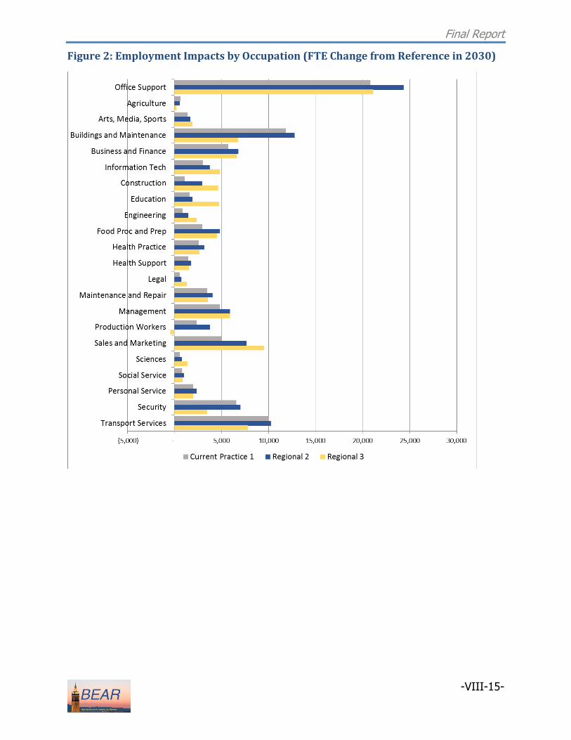
One of the salient features of the BEAR model is the ability to forecast employment impacts by occupation. In Figure 2 we present the employment impacts (relative to the 33% RPS reference scenario) by occupation across the different scenarios. Significant gains in employment span a variety of diverse sectors, signaling the large scope of indirect and induced effects from increasing the RPS. For example, while we find large increases in employment sectors readily associated with a large renewable build out such as construction, there are also large projected increases in sectors that are much less direct such as office support, sales and marketing, and food processing and preparation. In Figure 3 we compare how Current Practice 1 compares to the two different regionalization scenarios, Regional 2 and Regional 3. Here we find that job creation increases universally across all categories for Regional 2 compared to Current Practice 1, while Regional 3 shows some categories with less jobs created than Current Practice 1. This finding is important as although all scenarios stimulate job creation in California (as seen in Figure 2), there are some large differences between the regionalization scenarios in which occupations are affected.

Final Report

-VIII-15-

Figure 2: Employment Impacts by Occupation (FTE Change from Reference in 2030)

Final Report

-VIII-16-

Figure 3: Employment Impacts by Occupation – Regionalization Comparison (FTE Change from Baseline in 2030)

For each of the occupation classes previously listed, job creation either occurs as a result of the renewable buildout or from ratepayer savings effects. In Figure 4 and Figure 5, we show the different job creation between scenarios for ratepayer savings induced jobs and jobs from the renewable buildout. Regional 2 produces the most jobs overall, with an increase of over 19,000 jobs compared to Current Practice 1. This large growth is led primarily from ratepayer savings induced jobs and increased renewable build in California. Comparing Current Practice 1 and Regional 3 we find that Regional 3 has an even larger increase in jobs generated by the ratepayer savings from reduced energy rates, but has less jobs overall compared to Regional 2 due to less renewable buildout job creation in solar from more out-of-state renewables procurement.

Final Report

-VIII-17-

Figure 4: Statewide Jobs Created by 2030

Figure 5: Difference in Statewide Jobs Created by 2030

Final Report

-VIII-18-

2. Impacts by Income Decile

Another notable feature of the BEAR model is the ability to forecast results across income deciles. Given that the benefits from an increased renewable buildout will not be uniformly disturbed across the population, this feature of the model is particularly relevant for this study. The results for income impacts by decile are listed in Figure 6. In general, we find that the largest share of increases across income deciles occur in the middle and upper income deciles, with the largest projected increases occurring in decile 7, 8, and 9 under Regional 3. Consistent with our other results, we find the largest increases across all income groups in Regional 3. These results are reflective of the fact that more out-of-state procurement and Regional ISO operations in Regional 3 will produce the lowest energy rates among all scenarios, resulting in higher household income across all deciles. The difference in statewide income across all deciles can be seen more clearly in Figure 7, which reports the difference in statewide income between Scenario 1 and Regional 2 and Regional 3. As seen in the figure, Regional 3 results in the largest income effect owing to the lower rates from full regionalization. Note however that these figures should not be interpreted as how much additional income each household in California will enjoy as a result of regionalization. Instead, those households that receive new jobs will receive the vast amount of new benefits, while other households will only see a small increase from ratepayer savings. Therefore, this figure is somewhat misleading as it averages out the benefits across all households, when in reality only a few will receive the majority of benefits. However as each utility has different rate classes and rate allocations, it is not feasible to do a rate allocation study for this detail of a study.

Final Report

-VIII-19-

Figure 6: Household Real Income Impact by Decile (Percent Change from Reference in 2030)

Figure 7: Difference in Statewide Income in Year 2030

Final Report

-VIII-20-

3. Sensitivity Analysis

The economic analysis includes one sensitivity analysis that is identical to the Current Practice 1 scenario except with a higher limit on net bilateral sales from CAISO entities (8000MW vs. 2000MW). The statewide macroeconomic impacts for sensitivity 1B are shown in Table 5. The positive economic impacts compared to Current Practice 1 are due to the higher levels of investments in in-state wind and solar resources, combined with greater ratepayer savings due to the higher export capacity. The two regionalization scenarios result in moderately lower levels of employment growth compared to the sensitivity 1B scenario. Regional 2 results in 1,212 fewer jobs created and Regional 3 results in 9,432 fewer jobs created. Similar results are observed for gross state product and real output. Despite slightly lower ratepayer savings than the two regionalization scenarios, the greater in-state investments due to the renewable buildout generate more jobs and in-state economic activity. It is important to note that this sensitivity is an extreme bookend to isolate the benefits of a regional market holding the level of export capability constant. Achieving this level of export capability under the current market structure is extremely unlikely given the operational and market barriers that exist in the West. Nonetheless, the statewide macroeconomic impacts of this sensitivity are presented here for completeness.

Table 5: Macroeconomic Impacts for Sensitivity 1B in 2030 (2015 $ billions unless noted)

1B – CP1 Regional 2 – 1B Regional 3 – 1B

Gross State Product 2.284 -0.595 -1.115 Real Output 3.607 -0.869 -1.332 Employment (,000 FTE) 20.560 -1.212 -9.432

Real Income 4.285 -0.168 3.609 State Revenue 0.792 -0.205 0.788

V. Conclusion Although we find that all renewables investment scenarios offer tremendous benefits to a wide group of occupations and income groups, regionalization offers benefits to the widest group of Californians. While this is an important finding on its own, the benefits of a regional market undoubtedly extend beyond California. Regionalization offers other states an opportunity to increase their own RPS providing both job creation and income benefits through ratepayer savings. The foundation developed in this study could be used by others to assess what would demonstrate the scope of ratepayer benefits beyond California, and especially with respect to states who might opt in or out of a given regional framework. Our current findings are

Final Report

-VIII-21-

based on a variety of assumptions regarding the coordination and renewable buildout of other states, but they do not elucidate potential benefits that might recruit other states to the regional initiative. Such an exercise would be valuable for political sustainability, but also to facilitate more optimal regional trading and transmission integration for states considering joining the Regional ISO.

VI. References AEE Institute, “California Advanced Energy Employment Survey,” prepared by BW

Research Partnership for the Advanced Energy Economy Institute, December 2014. El Alami, Karim, and Daniel Kammen, “Green Job Creation and Regional Economic

Opporunties at the State Level, University of California, Berkele, Renewable & Appropriate Energy Laboratory, April 2015.

Jones, Betony, Peter Philips, and Carol Zabin, “Job Impacts of California’s Existing Proposed

Renewables Portfolio Standard - California,” University of California, Berkeley, Donald Vial Center on Employment in the Green Economy, August, 2015.

Kahle, David and Hadley Wickham. ggmap: Spatial Visualization with ggplot2. The R

Journal, 5(1), 144-161. http://journal.r-project.org/archive/2013-1/kahle-wickham.pdf

Philips, Peter, “Environmental and Economic Benefits of Building Solar in California:

Quality Careers – Cleaner Lives,” University of California, Berkeley, Donald Vial Center on Employment in the Green Economy, November, 2014.

Roland-Holst, David. 2015. “Berkeley Energy And Resources (BEAR) Model - Technical

Documentation for a Dynamic California CGE Model for Energy and Environmental Policy Analysis.”

bearecon.com