senior design project 2017, team 21, final report … report.pdf · senior design project 2017,...
TRANSCRIPT

SENIOR DESIGN PROJECT 2017, TEAM 21, FINAL REPORT 1
Electromagnetic Soil Moisture Sensor (ESMS)
Final Report
Kyle Richard, Nicholas Keith, Erik Sprague, Mohamed A. Mohamed
Abstract – Electromagnetic Soil Moisture Sensor is an
electromagnetic system that allow users to map moisture
levels over a small area of soil. It detects the power of the
electromagnetic energy radiated from the soil using an
antenna. Soil moisture is a key variable in controlling
water and heat energy between the land surface and the
atmosphere. Therefore, soil moisture plays an important
role in the development of weather patterns. The signal
captured is then fed into a Radio Frequency (RF)
receiver, where it’s amplified and filtered. The filtered
data is then saved on a micro SD card. The data in the
SD card is processed in a computer to produce a position
vs. brightness temperature map of the landscape.
Index Terms – Radiometry, Emissivity, Brightness
Temperature
I. INTRODUCTION
SUSTAINABILITY is a social movement that
aims to create a human lifestyle that preserves the earth’s
natural resources. We now live in a modern, consumerist,
and largely urban existence throughout the developed world,
where we consume a lot of natural resources every day. One
of these largely consumed resources is water. One of the
most urgent challenges facing our world today is ensuring an
adequate supply and quality of water in light of our
increased need and climate change. The agricultural sector
consumes about 70% of the planet’s accessible freshwater –
more than twice that of industry (23%), and municipal use
(8%) [8]. ESMS will help farmers reduce water waste
significantly, by allowing farmers to distribute water
efficiently across their landscapes.
A. Current Solutions
The most effective current solutions involve
radiometers or radar systems [1]. The premise of this is that
water in soil decreases the soil’s emissivity. Power radiated
is proportional to brightness temperature: P=KTBB, where K
is Boltzmann’s constant, TB is brightness temperature and B
is bandwidth. TB = e*T, where e is emissivity and T is the
true temperature. Soil of the same temperature with different
water content will radiate different power levels. By
directing an antenna at a certain area and measuring the
power received, the brightness temperature of that area can
be determined. This is also known as the “antenna
temperature.”
NASA developed such a system. They launched the
Soil Moisture Active Passive (SMAP) mission on January
31, 2015 [2]. The SMAP system consists of a radar and a
radiometer system that penetrates into the top 2 inches of the
soil. This mission will improve climate and weather
forecasts and allow scientists to monitor droughts and
predict floods and storms earlier and better. However, it was
built on large scale to see moisture levels across continents
using satellites.
Handheld moisture sensors have also been built that
require their user to place a pin into the soil to get a moisture
reading, but this method is both tiresome and time-
consuming. It is mainly used in construction to check
moisture levels under construction sites. These tools are not
always accurate and are not very efficient for farms.
B. Our Solution
To make radiometer technology more available to
users on a small scale, we would like to make a radiometer
system that could be mounted on a tractor or a drone. The
ideal case would be a drone-mounted system, but we will
prioritize the radiometric aspect and mount it to a drone if
time permits.
With our project, a small-scale farmer could be able
to map out the moisture in his or her fields. Using this
information, the farmer can optimize their irrigation system
and save water. During a time where water is becoming
more scarce, especially in the western part of the country,
this could mitigate the necessity for limitations on water use
in areas experiencing drought.
Additionally, our project could be used by
companies hoping to do construction on previously
untouched lands. The ESMS may be used to quickly
determine whether the land of interest is a wetland, which
would save time and money for the owner of the land and
the construction company.

SENIOR DESIGN PROJECT 2017, TEAM 21, FINAL REPORT 2
C. Specifications
Figure 1 lists the specifications for ESMS. The
specifications include operation time, system weight, and
measurement precision. We anticipate that our system will
be drawing 352 mA from a 11.1 V battery. The battery has a
capacity of 22mA hours, therefore our system could operate
for 6 hours. The reason for having an operation time of 30
minutes is that in the ideal case that the system is mounted to
a drone, the drone would likely not be able to fly with a
large payload for more than 30 minutes. The heavier the
payload of a drone, the shorter the flight time. This leads
into the overall system weight specification, we want to
build a system that is less than 3kg. After researching we
discovered there are drones that have the ability to fly for 30
min while carrying this payload. The last specification is
radiometric sensitivity of less than 1 kelvin. Meaning our
radiometer would be able to measure brightness temperature
to the accuracy of 1 kelvin. Brightness temperature is
proportional to the percentage of water in the soil. A study
done at Purdue University, called Soil Moisture Sensing
with Microwave Radiometers, researched the connection
between soil moisture and brightness temperature. In the
experiment they measured a bare field with a relatively
smooth surface. For comparison purposes they measure this
field at wet and dry conditions. There was about a 70k
difference for a 14 % difference in the soil moisture.
Meaning every 1% change in water concentration is
equivalent to a brightness temperature change of 5K.
System Requirements Specs
Operation Time 30 min
System Overall Weight < 3kg
Measurement Precision ΔT < 5 Kelvin
Figure 1. ESMS System Requirements
II. DESIGN
Figure 2 shows our system block diagram. The
major components comprising our project are an RF
receiver, a control circuit, various sensors to collect data,
and a power supply. The RF receiver consists of an antenna,
a circuit to amplify and filter the antenna signal, and a power
detector which produces a DC output voltage from which the
received signal’s input power may be determined. This
voltage will be sampled by our microcontroller along with
readings from two reference sources. The data will be stored
in an SD card and placed into a computer program after
collection. The program will utilize the power readings from
the antenna and two reference sources to determine the
antenna temperature. Soil with a high moisture content will
cause a lower antenna temperature, and that with a low
moisture content will cause a higher reading.
Figure 2. System Block Diagram
1. RF Antenna and Receiver
For the antenna, we acquired a microstrip-patch
antenna from the MIRSL (Microwave Instructional Remote
Sensing Laboratory). Designing a microstrip patch antenna
from scratch is very time-consuming, and building an
antenna is not the primary intent of our project. We
conducted analysis on the antenna we acquired to measure
its characteristics. The structure of the antenna consists of
two metal electrodes with a dielectric layer sandwiched
between them. We will build an L-band radiometer (1 - 2
GHz). Therefore, we want our antenna to resonate within
that band. Figure 3 shows the microstrip patch antenna we
used. L and W represent the length and width of each patch,
and h is the thickness of the dielectric material. For the
antenna, we have L=W= 6.85 cm, and h = 0.2 cm.
Figure 3. 2x2 Microstrip Patch Antenna
SENIOR DESIGN PROJECT 2017, TEAM 21, FINAL REPORT 3
The equation for the resonant frequency of the
patch antenna is:
𝑓0 =𝐶
2𝐿√𝜀𝑟
where c is the speed of light, L is the patch length, and ϵr is
the relative permittivity of the dielectric, ϵr = 2.406.
To determine the different antenna parameters, we
measured them using an HP Agilent network analyzer in the
MIL lab to look at S11. Figure 4 shows the S11 parameters
when the four patches are connected to the network
analyzer. The first minimum point shows the measured
resonant frequency to be f = 1.412 GHz with a BW= 20
MHz. Since the antenna has a resonant frequency of 1.412
GHz, it falls within the Radio Astronomy Band: 1.4-1.427
GHz. This means that we do not have to worry about Radio
Frequency Interference (RFI) with cell phones and other
devices with our antenna.
Figure 4. S11 vs. frequency showing 1.412 GHz as the
resonant frequency
The reason why we see a second minimum point at
almost double the initial frequency is because this is a multi-
band antenna, meaning that it can resonate at different
frequencies for different applications. However, since we are
working in L-band, we are only interested in the first one
and the second one will be filtered out using a bandpass
system in the receiver circuit.
The receiver circuit consists of a cascade of a low-
noise amplifier (LNA), bandpass filter, and a power
amplifier (PA). We know that the ambient noise floor, tested
a matched load, is about -75 dBm at room temperature. We
know that we want our signal to be well above the noise
floor, so we estimated that a ballpark of 40-50 dB of gain
would be adequate. We received amplifiers and a bandpass
filter from the MIRSL lab to test out the functionality and
gain an understanding of the radiometer circuit. The
bandpass filter is paired with the antenna; it has the same
bandwidth and center frequency. When we connect the LNA
to the bandpass filter to the PA and view the output on the
spectrum analyzer, we see the shape of the filter’s frequency
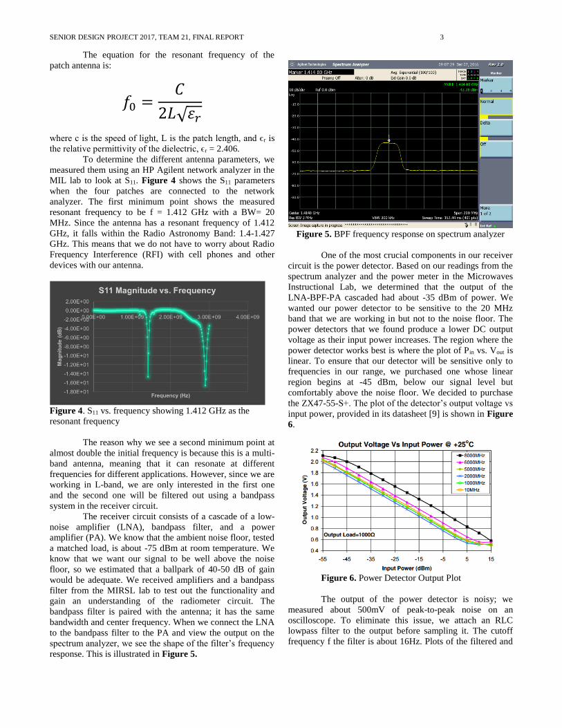
response. This is illustrated in Figure 5.
Figure 5. BPF frequency response on spectrum analyzer
One of the most crucial components in our receiver
circuit is the power detector. Based on our readings from the
spectrum analyzer and the power meter in the Microwaves
Instructional Lab, we determined that the output of the
LNA-BPF-PA cascaded had about -35 dBm of power. We
wanted our power detector to be sensitive to the 20 MHz
band that we are working in but not to the noise floor. The
power detectors that we found produce a lower DC output
voltage as their input power increases. The region where the
power detector works best is where the plot of Pin vs. Vout is
linear. To ensure that our detector will be sensitive only to
frequencies in our range, we purchased one whose linear
region begins at -45 dBm, below our signal level but
comfortably above the noise floor. We decided to purchase
the ZX47-55-S+. The plot of the detector’s output voltage vs
input power, provided in its datasheet [9] is shown in Figure
6.
Figure 6. Power Detector Output Plot
The output of the power detector is noisy; we
measured about 500mV of peak-to-peak noise on an
oscilloscope. To eliminate this issue, we attach an RLC
lowpass filter to the output before sampling it. The cutoff
frequency f the filter is about 16Hz. Plots of the filtered and

SENIOR DESIGN PROJECT 2017, TEAM 21, FINAL REPORT 4
unfiltered output are compared in Figure 7a and Figure 7b,
respectively.
Figure 7a. Unfiltered Detector Output
Figure 7b. Filtered Detector Output
2. Control circuit
To calibrate our system properly, we need receiver
output readings and temperature readings of our reference
sources for each sample. The GPS receiver has a data rate of
10Hz, which sets the upper limit for the data rate of the rest
of our system. We count a “supersample” as a receiver
output reading from the antenna and each reference source
and, the temperatures of the reference sources, which is five
analog readings in total. Each of these supersamples will be
stamped with a location and time from the GPS receiver.
The microcontroller will also have to change the switch
control logic using its GPIO pins in between receiver
samples. Since all of this will only be happening around 10
Hz, this is not a hard requirement to meet.
The control circuit will determine if the switch
outputs the antenna or the reference sources, it will sample
the outputs from each sensor, and record all data to the SD
card. Initially we wanted to take supersamples at 10Hz, once
every 100ms, but the settling time of the low pass filter is
only 62.5ms. Since each source (antenna, noise diode,
matched load) must be sampled within a supersample, and
we cannot sample faster than the filter’s settling time, the
slowest data rate for supersamples would be 3*62.5ms =
187.5ms. We decided to go with an even number and sample
a source every 65ms, giving a supersample time of 195 ms.
We chose the Arduino Mega 2560 [10] to function
as our control circuit. The Arduino comes with 54 I/O pins
and 16 analog inputs, which will be used to coordinate
switching and sample the sensor outputs. Another advantage
of the Arduino Mega 2560 is that there are various breakout
boards that can easily be incorporated with it. We purchased
a GPS breakout board and an SD breakout board which both
can be simply connected to the Arduino. The Arduino
software is easy to learn how to use and program our own
code. With a 16MHz processor, it has the ability to take the
samples and coordinate the messages laid out in the previous
paragraph.
The analog to digital converter (ADC) can limit our
radiometric sensitivity, so its resolution must not put the
sensitivity below 5K. To find the limit set by the ADC,
simply find the change in power corresponding to an
increase of one-bit level at the detector output, and convert
this to a brightness temperature with the P=KTB relation.
We found that with the stock 10-bit ADC included with our
Arduino, our sensitivity was 6.4K. To improve this, a 15-bit
ADC breakout board was purchased. This changed the
radiometric sensitivity limit set by the ADC to 0.38K.
3. Data Processing
To conserve computing power and make the design
simpler, we will do all of our data processing after collection
on a PC. A program will be required to read the data on the
SD card line by line and run an algorithm to calculate the
brightness temperatures that we need.
To understand our data, we need to create a lookup
table of detector output voltage vs. input power. Figure 4,
the plot provided in the datasheet, provides a rough idea of
these values. However, more accurate numbers will be
required to make calculations. A lookup table will be
developed using technology in the MIL lab. A signal
generator will be used to increase the input power to the
detector in small increments, while a multimeter will record
the output voltage. The data will be stored in an excel file
and used later by the processing algorithm.
Our reference sources, a matched load and a noise
source, are critical components. The program will first
convert the recorded receiver output voltage to an input
power, based on values from the lookup table. Resistive
temperature detectors (RTD), which are devices whose
resistance changes based on their temperature, will be used
to find the temperature of each reference source. Since we
will not be working in extreme temperatures, mostly any
SENIOR DESIGN PROJECT 2017, TEAM 21, FINAL REPORT 5
RTD with a large dynamic range will suffice. The matched
load produces the same noise power as is expected, P =
KTB. The noise source, however, has a high Equivalent
Noise Ratio (ENR). This means that it produces noise that is
equal to the product of KTB and its ENR; it will radiate
power as though it was much hotter than its actual
temperature. We will multiply the measured temperature of
the noise source by the ENR to find what temperature it
appears to be, radiometrically. Since power has a linear
relationship to temperature, our values of temperature and
detector input power combined form a line on a temperature
vs. power plot. By finding the point on this line where the
measured antenna output power lies, the antenna
temperature can be extrapolated. This calibration process
will be carried out for every supersample.
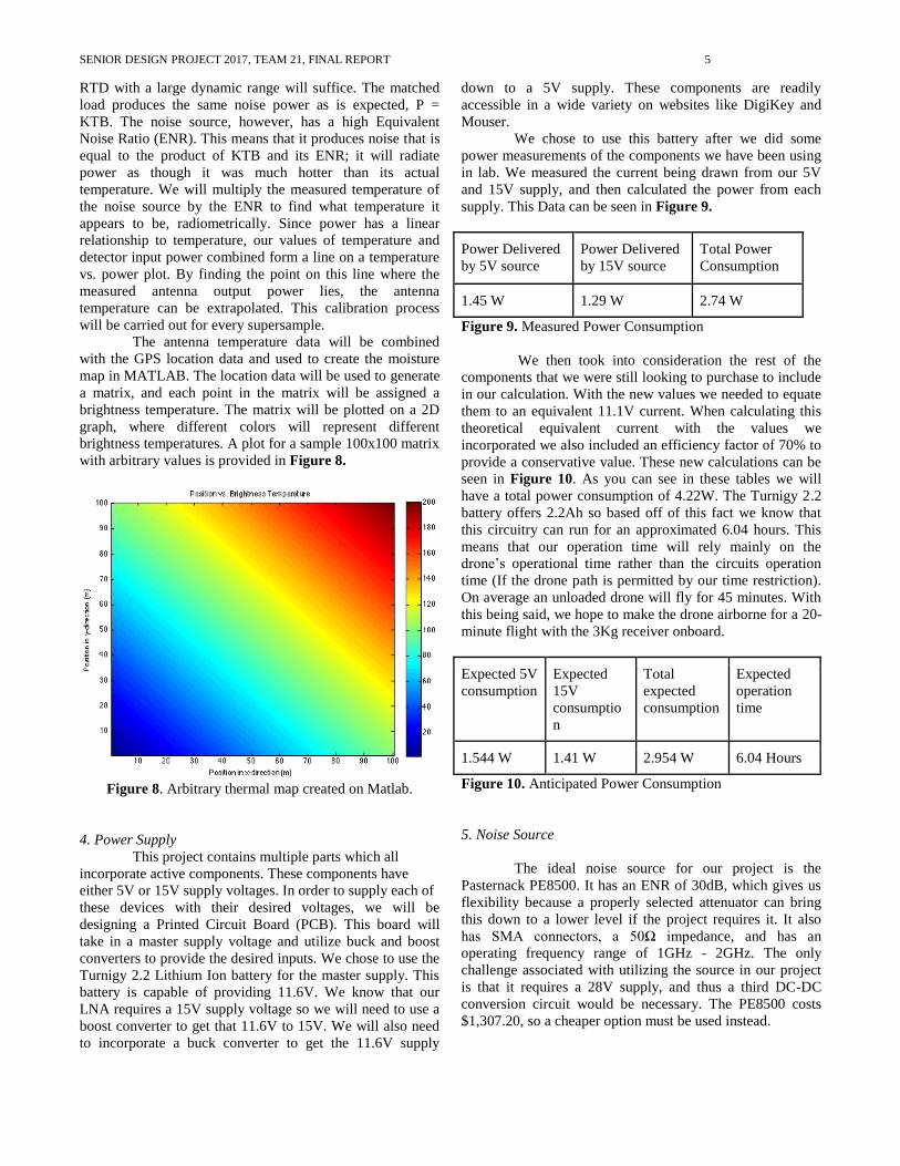
The antenna temperature data will be combined
with the GPS location data and used to create the moisture
map in MATLAB. The location data will be used to generate
a matrix, and each point in the matrix will be assigned a
brightness temperature. The matrix will be plotted on a 2D
graph, where different colors will represent different
brightness temperatures. A plot for a sample 100x100 matrix
with arbitrary values is provided in Figure 8.
Figure 8. Arbitrary thermal map created on Matlab.
4. Power Supply
This project contains multiple parts which all
incorporate active components. These components have
either 5V or 15V supply voltages. In order to supply each of
these devices with their desired voltages, we will be
designing a Printed Circuit Board (PCB). This board will
take in a master supply voltage and utilize buck and boost
converters to provide the desired inputs. We chose to use the
Turnigy 2.2 Lithium Ion battery for the master supply. This
battery is capable of providing 11.6V. We know that our
LNA requires a 15V supply voltage so we will need to use a
boost converter to get that 11.6V to 15V. We will also need
to incorporate a buck converter to get the 11.6V supply
down to a 5V supply. These components are readily
accessible in a wide variety on websites like DigiKey and
Mouser.
We chose to use this battery after we did some
power measurements of the components we have been using
in lab. We measured the current being drawn from our 5V
and 15V supply, and then calculated the power from each
supply. This Data can be seen in Figure 9.
Power Delivered
by 5V source
Power Delivered
by 15V source
Total Power
Consumption
1.45 W 1.29 W 2.74 W
Figure 9. Measured Power Consumption
We then took into consideration the rest of the
components that we were still looking to purchase to include
in our calculation. With the new values we needed to equate
them to an equivalent 11.1V current. When calculating this
theoretical equivalent current with the values we
incorporated we also included an efficiency factor of 70% to
provide a conservative value. These new calculations can be
seen in Figure 10. As you can see in these tables we will
have a total power consumption of 4.22W. The Turnigy 2.2
battery offers 2.2Ah so based off of this fact we know that
this circuitry can run for an approximated 6.04 hours. This
means that our operation time will rely mainly on the
drone’s operational time rather than the circuits operation
time (If the drone path is permitted by our time restriction).
On average an unloaded drone will fly for 45 minutes. With
this being said, we hope to make the drone airborne for a 20-
minute flight with the 3Kg receiver onboard.
Expected 5V
consumption
Expected
15V
consumptio
n
Total
expected
consumption
Expected
operation
time
1.544 W 1.41 W 2.954 W 6.04 Hours
Figure 10. Anticipated Power Consumption
5. Noise Source
The ideal noise source for our project is the
Pasternack PE8500. It has an ENR of 30dB, which gives us
flexibility because a properly selected attenuator can bring
this down to a lower level if the project requires it. It also
has SMA connectors, a 50Ω impedance, and has an
operating frequency range of 1GHz - 2GHz. The only
challenge associated with utilizing the source in our project
is that it requires a 28V supply, and thus a third DC-DC
conversion circuit would be necessary. The PE8500 costs
$1,307.20, so a cheaper option must be used instead.
SENIOR DESIGN PROJECT 2017, TEAM 21, FINAL REPORT 6
A cheaper option is the Noisecom NC302 noise
diode. It is easily configured with the 15V supply, and
Noisecom generously gave us three free samples of the
NC302. We are having difficulties feeding the signal from
the pins of the NC302 to our SMA connected system, which
is a disadvantage compared to the PE8500, but to stay within
budget and avoid designing a third DC-DC converter, we
use the NC302.
III. PROJECT MANAGEMENT
Through consistent communication and
collaboration our team has worked as a cohesive group since
the beginning of this project. We communicate using a
group text message to schedule weekly meetings and set
times to work together on the project. We meet weekly with
Professor Frasier to update him on the project status and ask
any questions that may arise. The subsystems of our project
are related and intertwined, so it is important that every
member of our team have an understanding of each aspect of
our system. Our team has done a great job at planning and
using each other to solve any problems. In order to ensure
we would meet our MDR deliverables we delegated specific
tasks to each member of the group. Nick and Kyle focused
on the receiver circuit including the radio frequency
amplifying, filtering, and converting the RF signal into a DC
voltage. We designated two people for this task because we
felt the receiver circuit was a major aspect of our project.
Erik focused on the control logic of our system including the
microcontroller interaction with the switch and the data
storage device. Mohamed focused on understanding the
antenna that was generously given to our group by Professor
Frasier. He also started working with Matlab to generate a
grid of soil moisture vs. location.
MDR Deliverables Status
RF circuit prototype Completed
Detect changes in
brightness temperature
Attempted, more definitive
proof needed
Store data in SD card Completed
Figure 11. MDR Deliverables
Since MDR, we have encased our project,
purchased a 4-way power combiner, and have been able to
collect data since we are no longer bound by the length of an
extension cord. At FPR, our GPS receiver was not working
well as we wanted it to, and therefore the data we presented
was not fully convincing. In the week between FPR and
demo day, we increased the precision of the data provided
by the GPS receiver and then worked hard to collect as much
brightness temperature data as possible. Without this
improvement in precision of the GPS data, our current
thermal maps would not be convincing enough to
demonstrate the project’s functionality.
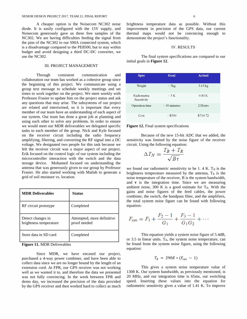
IV. RESULTS
The final system specifications are compared to our
initial goals in Figure 12.
Figure 12. Final system specifications
Because of the new 15-bit ADC that we added, the
sensitivity was limited by the noise figure of the receiver
circuit. Using the following equation:
we found our radiometric sensitivity to be 1. 4 K. TB is the
brightness temperature measured by the antenna, TR is the
noise temperature of the receiver, B is the system bandwidth,
and τ is the integration time. Since we are measuring
ambient noise, 300 K is a good estimate for TB. With the
gains and noise figures of the feed cables, the power
combiner, the switch, the bandpass filter, and the amplifiers,
the total system noise figure can be found with following
equation:
This equation yields a system noise figure of 5.4dB,
or 3.5 in linear units. TR, the system noise temperature, can
be found from the system noise figure, using the following
equation:
𝑇𝑅 = 290𝐾 ∗ (𝐹𝑐𝑎𝑠 − 1)
This gives a system noise temperature value of
1308 K. Our system bandwidth, as previously mentioned, is
20 MHz, and our integration time is 65ms, our switching
speed. Inserting these values into the equation for
radiometric sensitivity gives a value of 1.41 K. To improve

SENIOR DESIGN PROJECT 2017, TEAM 21, FINAL REPORT 7
this number even further, we used a 3 sample moving
average on the power values from each source in watts,
which increased the integration time to 195 ms. This change
brought the sensitivity to 0.81 K.
To test how our system would detect differences in
measured brightness temperature between soils of different
moistures, we suspended the system in one location over wet
and dry soil for two minutes each. Figure 13 shows
measured temperature of the dry spot vs. time, and Figure
14 shows the same for wet soil. The measured mean
brightness temperature was 243.5K for the dry soil, and
228.9K for the wet soil.
Figure 13. Brightness temperature over a dry spot
Figure 14. Brightness temperature over a wet spot
This data was saved on a micro SD card along with
GPS coordinates and the ambient temperature. The
difference we measured in brightness temperature shows that
our system is capable of detecting changes in the power that
is being radiated. The saved data was then processed on
matlab to produce a map of brightness temperature over a
given area. The path we walked can be seen as a scatterplot
in Figure 15. This scatterplot is then interpolated to produce
the thermal map that can be seen in Figure 16.
Figure 15. Scatter plot of brightness temperature of a farm
in South Amherst
Figure 16. Interpolated plot of scatter data
Our system was contained inside a wooden box
with a plexiglass cover. This cover allowed the GPS unit to
receive a satellite fix while protecting the inner RF
components as shown in Figure 17. The dimensions were
measured to be an exact match to the size of the antenna
allowing it to be mounted on the bottom of the box as can be
seen in Figure 3.
Figure 17. Full System encasing
The antenna seen in Figure 3 was simulated in
HFSS software to find its radiation pattern. The half power
beam width was found to be 60°. Using this value, we
calculated the area covered by the antenna in its far field to
be roughly 104 sq ft. This was calculated using the fact that
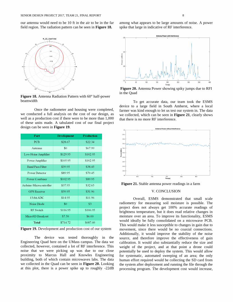
SENIOR DESIGN PROJECT 2017, TEAM 21, FINAL REPORT 8
our antenna would need to be 10 ft in the air to be in the far
field region. The radiation pattern can be seen in Figure 18.
Figure 18. Antenna Radiation Pattern with 60° half-power
beamwidth
Once the radiometer and housing were completed,
we conducted a full analysis on the cost of our design, as
well as a production cost if there were to be more than 1,000
of these units made. A tabulated cost of our final project
design can be seen in Figure 19.
Figure 19. Development and production cost of our system
The device was tested thoroughly in the
Engineering Quad here on the UMass campus. The data we
collected, however, contained a lot of RF interference. This
noise that we were picking up was due to our close
proximity to Marcus Hall and Knowles Engineering
building, both of which contain microwaves labs. The data
we collected in the Quad can be seen in Figure 20. Looking
at this plot, there is a power spike up to roughly -22dB
among what appears to be large amounts of noise. A power
spike that large in indicative of RF interference.
Figure 20. Antenna Power showing spiky jumps due to RFI
in the Quad
To get accurate data, our team took the ESMS
device to a large field in South Amherst, where a local
farmer was kind enough to let us test our system in. The data
we collected, which can be seen in Figure 21, clearly shows
that there is no more RF interference.
Figure 21. Stable antenna power readings in a farm
V. CONCLUSION
Overall, ESMS demonstrated that small scale
radiometry for measuring soil moisture is possible. The
project does not always get 100% accurate readings of
brightness temperature, but it does read relative changes in
moisture over an area. To improve its functionality, ESMS
would ideally be fully consolidated on a microwave PCB.
This would make it less susceptible to changes in gain due to
movement, since there would be no coaxial connections.
Additionally, it would improve the stability of the noise
source, and therefore improve the effectiveness of gain
calibration. It would also substantially reduce the size and
weight of the project, and at that point a drone could
potentially be used to deploy the system. This would allow
for systematic, automated sweeping of an area; the only
human effort required would be collecting the SD card from
the system after deployment and running the file through the
processing program. The development cost would increase,
SENIOR DESIGN PROJECT 2017, TEAM 21, FINAL REPORT 9
but after completion the system would be easier to mass-
produce.
VI. ACKNOWLEDGEMENTS
We would like to give a special thanks to our
advisor, professor Frasier, for lending us his continuous
guidance as well as providing inspiration for the project. We
would also like to thank Professors Vouvakis and Anderson
for their helpful and constructive criticism that led to system
improvements. Also, we want to thank Professor Hollot for
guiding us in the right direction throughout the year. Finally,
a special thanks to NoiseComm for donating parts to our
project.
VII. REFERENCES
[1] Schmugge, T. "Remote Sensing of Soil Moisture with
Microwave Radiometers." Transactions of the ASAE 26.3
(1983): 0748-753
[2] Acevo-Herrera, Rene, Albert Aguasca, Xavier Bosch-
Lluis, Adriano Camps, José Martínez-Fernández, Nilda
Sánchez-MartÃn, and Carlos Pérez-Gutiérrez. "Design and
First Results of an UAV-Borne L-Band Radiometer for
Multiple Monitoring Purposes." Remote Sensing 2.7 (2010):
1662-679
[3] Pozar, David M. "Microwave Engineering Education:
From Field Theory to Circuit Theory."2012 IEEE/MTT-S
International Microwave Symposium Digest (2012): n. pag
[4] Bevelacqua, Pete. "Microstrip (Patch) Antennas."
Microstrip Antennas: The Patch Antenna. N.p., n.d. Web
[5] Koivu, S. "Unknown Signal Detection Using a Digital
Total-Power Radiometer with Finite Internal Precision."
2006 IEEE Instrumentation and Measurement Technology
Conference Proceedings (2006): n. pag
[6] "Brightness Temperature in Monitoring of Soil
Wetness." SpringerReference (n.d.): n. pag
[7] "Microstrip Antenna Array." Microstrip Patch Antennas
(2010): 487-515
[8] Farming: Wasteful Water Use." WWF. WWF Global,
n.d. Web
[9] Mini-Circuits, “Power Detector: -55dBm to +10dBm,”
ZX47-55 datasheet, Rev. D
[10] Atmel, “8-bit Atmel Microcontroller with 16/32/64KB
In-System Programmable Flash” Feb, 2014
[11] Pozar, David M. Microwave engineering. 4th ed.
Hoboken, NJ: Wiley, 2012. Print.