sensitivity analysis of catch-per-unit-effort of atlantic bigeye tuna ... · palabras clave:...

Stock assessment of Atlantic bigeye tuna 1

Lat. Am. J. Aquat. Res., 43(1): 146-161, 2015

DOI: 10.3856/vol43-issue1-fulltext-13

Research Article

Sensitivity analysis of catch-per-unit-effort of Atlantic bigeye tuna

(Thunnus obesus) data series applied to production model

Humber A. Andrade1

1Universidade Federal Rural de Pernambuco (UFRPE) Departamento Pesca e Aquicultura (DEPAq)

Av. Dom Manoel de Medeiros s/n, Dois Irmãos, CEP 52171-030, Recife-PE, Brazil Corresponding author: Humber A. Andrade ([email protected])

ABSTRACT. Different datasets and a Bayesian production model were used to assess the status of the Atlantic

bigeye tuna (Thunnus obesus) stock. Several datasets convey little information hence estimations of parameters are imprecise unless a very restrictive prior is used. Modes of posteriors calculated for composite datasets are in

between modes of the posteriors calculated for separated datasets. Most of the calculations indicate that biomass has decreased until the beginning of 1990’s when the stock was overfished. Catches decreased after 1999 but

there is doubt if the stock was recovering in 2000’s. The answer depends on the dataset and on the prior distribution.

Keywords: stock assessment, biomass, production model, Bayesian model, adaptive importance sampling.

Análisis de sensibilidad de la captura por unidad de esfuerzo del atún patudo del

Atlántico (Thunnus obesus) con series de datos aplicados a un modelo de producción

RESUMEN. Diferentes conjuntos de datos y un modelo bayesiano de producción fueron utilizados para evaluar el stock del atún patudo del Atlántico (Thunnus obesus). Varios conjuntos de datos transmiten poca información

por lo tanto las estimaciones de los parámetros son imprecisas, salvo que se utilice una distribución a priori muy restrictiva. Las modas de las a posteriori calculadas para conjuntos de datos compuestos están entre las modas

de las a posteriori calculadas para conjuntos de datos separados. La mayoría de los cálculos indica que la biomasa ha disminuido hasta principios de los 90 cuando el stock fue sobreexplotado. Las capturas disminuyeron

después de 1999, pero hay dudas sobre si el stock se estaba recuperando en los años 2000. La respuesta depende del conjunto de datos y de la distribución a priori utilizada.

Palabras clave: evaluación de stock, biomasa, modelo de producción, modelo bayesiano, muestreo adaptable

por importancia.

INTRODUCTION

Bigeye tuna (Thunnus obesus) are distributed

throughout the Atlantic Ocean between 50ºN and 45ºS,

but not in the Mediterranean Sea (ICCAT, 2010).

Evidences, such as lack of identified genetic hetero-

geneity and the time-area distribution of fish and

movements of tagged fish, suggest an Atlantic-wide

single stock, which is currently the hypothesis accepted

by the International Commission for Conservation of Atlantic Tunas (ICCAT).

In the Atlantic Ocean catches of bigeye are high if

compared to catches of other tuna species. Only catches

of the smaller and less valuable skipjack (Katsuwonus

___________________

Corresponding editor: José A. Alvarez

pelamis) and yellowfin tuna (Thunnus albacares) are

higher than those of bigeye. Most of the bigeye has

been caught by longliners but the species is also caught

by bait-boat and purse-seine vessels (Miyake et al.,

2004; ICCAT, 2010). Several countries fish bigeye in

the Atlantic Ocean but catches of Japan, Taiwan, Ghana

and Spain were the higher ones in the last decade

(ICCAT, 2010).

In the last three stock assessment analyses for

bigeye tuna carried out by ICCAT Working Group

(ICCAT WG) both simple (e.g., production models-

Schaefer, 1954) and complex models (e.g., fully

integrated Stock Synthesis-(Method, 1990)) were used (ICCAT, 2005, 2008, 2011). ICCAT WG noticed there

146

mailto:[email protected]

2 Latin American Journal of Aquatic Research

were considerable uncertainty concerning data and

methods; consequently, estimations of benchmarks

were very different. For example, maximum sustain-

nable yield varied between 70,000 and 90,000 ton.

Regarding methods complex models are more realistic,

but simple models can be useful when data is limited

(Ludwig & Walters, 1985). Bayesian and conventional

versions of simple production models are often used.

Discussions about the limitations and the usefulness of

production models can be found in Prager (2002),

Maunder (2003) and Prager (2003).

Several datasets from different countries concerning

different gears and vessels are available for analysis of

the bigeye stock. Relative abundance indexes

calculated for different fleets are available in the last

stock assessment meeting report (ICCAT, 2011). In

some situations those multiple series of indexes are

analyzed separately, but analyzing them together and

composite indexes are also alternatives adopted by

ICCAT WG. However Richards (1991) suggests that

the analyses might be conducted separately for each

dataset and the results should be presented separately to

the decision makers. Following the same line of

reasoning Schnute & Hilborn (1993) provided a

composite model structure that allows the information

conveyed by each separated dataset to arise in the

results. Hence the objective here is to assess what are

the results if we look at separated relative abundance

datasets in the case of the Atlantic bigeye. Comparisons

with the results gathered when analyzing composite indexes are warranted.

A Bayesian version of the production model was

used because it allows previous knowledge about the

fish stock to be considered in the analysis. For further

comments on the use of Bayesian approach in fish stock

assessment see Punt & Hilborn (1997), McAllister &

Kirkwood (1998) and Meyer & Millar (1999a). Several

methods can be used to calculate the posterior

distributions in the Bayesian approach. Analytical

solutions may be difficult to achieve hence Monte

Carlo approaches are the alternative. Numerical

methods like Markov Chain Monte Carlo (MCMC) and

importance sampling methods are often used (Berger,

1985; Oh & Berger, 1992; West, 1993). Some authors

have argued that MCMC is less efficient than

importance sampling methods (Smith, 1991; Givens,

1993) though Meyer & Millar (1999a, 1999b) have

showed that Gibbs sampler can be efficient even when

there are many parameters. Nevertheless, MCMC may

not converge when the posterior is multimodal (Newton

& Raftery, 1994). Among the sampling importance methods the Sampling Importance Resampling (SIR)

was the more popular in fishery stock assessments

studies carried out in 1990's (e.g., Raftery et al., 1995;

McAllister & Ianelli, 1997; McAllister & Kirkwood,

1998). Successful application of the importance

sampling methods depends on the skill to build an

importance function that is easy to sample from and

similar to the posterior but with heavier tails (Van Dijk

& Kloek, 1983; Oh & Berger, 1992). In this paper

Adaptive Importance Sampling (AIS) was used

because it is an iterative procedure in which a finite

mixture of multivariate probability density functions is

automatically updated until a suitable importance

function is achieved (West, 1993). Applications of AIS

in fisheries analyses can be found in Kinas (1996) and Andrade & Kinas (2007).

MATERIALS AND METHODS

Catch and relative abundance indexes

Catches of bigeye in the Atlantic are shown in Figure 1. There was an increasing trend since commercial

fishery began in the 1950’s. After the peak in 1994

catches have decreased until 2002 and since then, there was no clear time trend. Catch-per-unit-effort (CPUE)

data from commercial fisheries are often used to calculate relative abundance indexes. Several proce-

dures can be used to “standardize” CPUE in order to obtain those indexes (Maunder & Punt, 2004).

Hereafter I assume to start that standardized CPUEs

appearing in the 2010 bigeye assessment meeting report are useful as relative abundance indexes. Those indexes

are shown in Table 1. Composite indexes were calculated using a generalized linear model with fleet

as factor (ICCAT, 2011). All the indexes time series are

shorter than the catch time series. However most of the indexes datasets cover a long period, though Morocco

time series is an exception (S6 in Table 1). Notice also that ICCAT WG have excluded some data in order to

calculate three of the composite time series (i.e., C4, C5

Figure 1. Catches of Atlantic bigeye tuna as reported in

the ICCAT 2010 bigeye assessment meeting. Catch for

2009 is the provisional estimation used in the meeting.

147


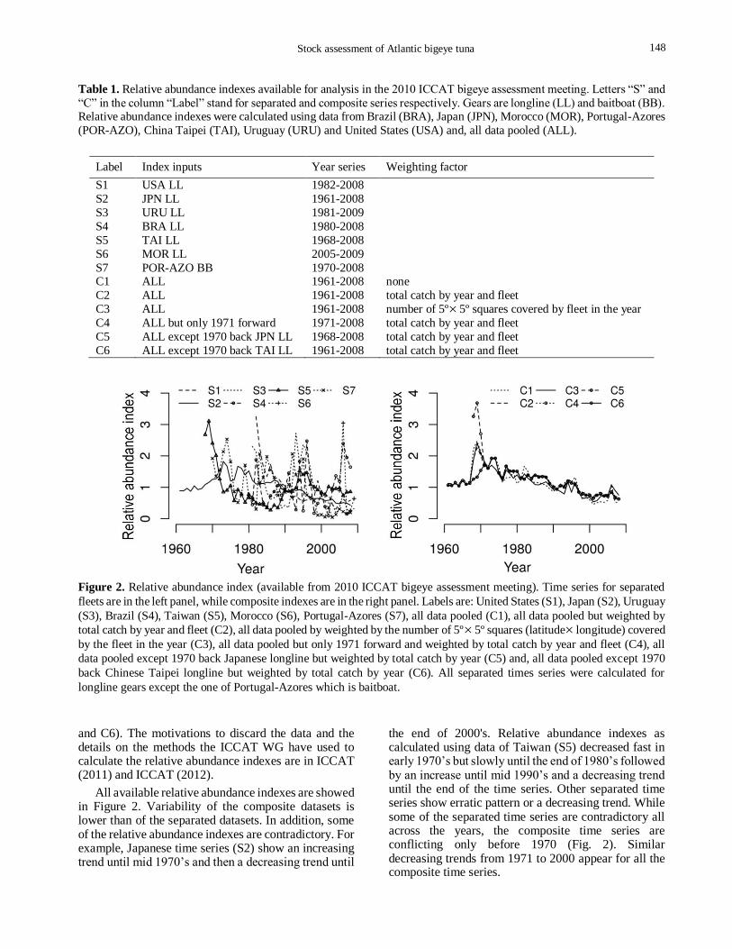
Table 1. Relative abundance indexes available for analysis in the 2010 ICCAT bigeye assessment meeting. Letters “S” and

“C” in the column “Label” stand for separated and composite series respectively. Gears are longline (LL) and baitboat (BB). Relative abundance indexes were calculated using data from Brazil (BRA), Japan (JPN), Morocco (MOR), Portugal-Azores

(POR-AZO), China Taipei (TAI), Uruguay (URU) and United States (USA) and, all data pooled (ALL).

Label Index inputs Year series Weighting factor

S1 USA LL 1982-2008

S2 JPN LL 1961-2008

S3 URU LL 1981-2009

S4 BRA LL 1980-2008

S5 TAI LL 1968-2008

S6 MOR LL 2005-2009

S7 POR-AZO BB 1970-2008 C1 ALL 1961-2008 none

C2 ALL 1961-2008 total catch by year and fleet

C3 ALL 1961-2008 number of 5º5º squares covered by fleet in the year

C4 ALL but only 1971 forward 1971-2008 total catch by year and fleet

C5 ALL except 1970 back JPN LL 1968-2008 total catch by year and fleet

C6 ALL except 1970 back TAI LL 1961-2008 total catch by year and fleet

Figure 2. Relative abundance index (available from 2010 ICCAT bigeye assessment meeting). Time series for separated

fleets are in the left panel, while composite indexes are in the right panel. Labels are: United States (S1), Japan (S2), Uruguay

(S3), Brazil (S4), Taiwan (S5), Morocco (S6), Portugal-Azores (S7), all data pooled (C1), all data pooled but weighted by

total catch by year and fleet (C2), all data pooled by weighted by the number of 5º5º squares (latitude longitude) covered

by the fleet in the year (C3), all data pooled but only 1971 forward and weighted by total catch by year and fleet (C4), all

data pooled except 1970 back Japanese longline but weighted by total catch by year (C5) and, all data pooled except 1970

back Chinese Taipei longline but weighted by total catch by year (C6). All separated times series were calculated for

longline gears except the one of Portugal-Azores which is baitboat.

and C6). The motivations to discard the data and the details on the methods the ICCAT WG have used to calculate the relative abundance indexes are in ICCAT (2011) and ICCAT (2012).

All available relative abundance indexes are showed in Figure 2. Variability of the composite datasets is lower than of the separated datasets. In addition, some of the relative abundance indexes are contradictory. For example, Japanese time series (S2) show an increasing trend until mid 1970’s and then a decreasing trend until

the end of 2000's. Relative abundance indexes as calculated using data of Taiwan (S5) decreased fast in early 1970’s but slowly until the end of 1980’s followed by an increase until mid 1990’s and a decreasing trend until the end of the time series. Other separated time series show erratic pattern or a decreasing trend. While some of the separated time series are contradictory all across the years, the composite time series are conflicting only before 1970 (Fig. 2). Similar decreasing trends from 1971 to 2000 appear for all the composite time series.

148


Stock assessment model

Catches and relative abundance indexes are the input

data for simple production models. Indexes are often

assumed to be proportional to abundance. I have

assumed the relationship between biomass (B) and

relative abundance indexes (I) in the tht year is:

v

tt eBqI (1)

Where v is a normally distributed random variable

with variance V , accounting for observational error.

Catchability coefficient q is assumed to be constant or,

at least, to change at random over the years. That

assumption holds if the standardization of CPUE was successful.

I have used the following version of traditional

logistic production model (Graham, 1935; Schaefer, 1954):

kBrBCBB ttttt 1111 1 (2)

Where tC is the catch in the tht year, r is the

population growth rate, k is the carrying capacity

biomass. Observation error in tC was assumed to be

negligible and the process error was not considered.

Aside the nuisance (V) there are three parameters of

interest: r , k and q . Because it is mathematically

more convenient to deal with parameters defined over

the real line let qkr log,log,log be the three

dimensional parameter vector of interest.

Bayesian approach

Bayesian inference of is obtained by the product of

prior probability density distribution π( ) and the

likelihood xL | calculated based on the data x . The

posterior density distribution for is:

xL

xLxp

|

||

(3)

In some cases there is not analytical solution for the

integral in the denominator. A couple of numerical

procedures can be used to obtain a sample of from a

distribution (importance function) that is assumed to be

similar to the true posterior xp | . When using such

numerical procedure it is necessary to verify if the

sample of indeed was drawn from an importance

function similar to the posterior distribution. Hereafter

the question about how close are the posterior and the importance function is denominated “convergence”.

Details about the solutions and equations I have used

are in Kinas (1996) and Andrade & Kinas (2007) but,

some explanations are warranted in the following sections.

Likelihood

After taking the logarithm of equation 1 and for

notational convenience, I define tt IY log and

tt qBlog . The probability model for tY is:

VNVYp tt ,~,| (4)

Where VN t , is an one-dimensional normal

distribution with mean t and varianceV . Let the

complete data set be YYY ,,1 , hence the joint

likelihood is VYpYVL ,||, . If indepen-

dent prior distributions are assumed for and for V,

say VV , , then the likelihood xL | is

obtained by marginalization with respect toV :

VVVYpxL d ,|| (5)

Kinas (1996) showed that if the prior for V is an

inverse-gamma density distribution, say ,~ IGV ,

the solution is:

2

1

22

2|

t

ttY

xL (6)

That choice about prior distribution for V is conve-

nient because the inverse-gamma is conjugated with the

normal probability in equation 5. The resulting

likelihood equation is simple in the sense that it only

depends on the residuals with respect to µt (ɵ) and on the prior parameters for V.

In order to calculate the likelihood (equation 6),

biomass in each year is estimated by using the equation

2. Nevertheless, an initial value of biomass for the first

year needs to be defined in advance. I have assumed the

initial biomass is equal to the carrying capacity k (i.e.,

kB 0) because catch was probably very small before

the first year to show up in the available time series

(Fig. 1). Furthermore, when kB 0 is assumed the

biases of estimations related to “maximum sustainable

yield” (MSY) are not large whenever the observational error is used to fit the model (Punt, 1990).

Prior

The priors for r and k used in this paper were based

mainly on priors the ICCAT WG have used in the

bigeye assessment meetings (e.g., ICCAT, 2005). In

2007 the ICCAT WG decided to use a uniform prior for

149


k bounded at 1.5x105 and 2.5x106 (ICCAT, 2008). The

informative prior for r was lognormal, with mean on

the original scale equal to 0.6, and standard deviation

on logarithm scale equal to 0.3 (e.g., SD(log r) = 0.3) in

2004 and 2007 stock assessments (ICCAT, 2005,

2008). In the 2010 assessment meeting the ICCAT WG

decided to use again priors similar to those used in the two previous meetings (ICCAT, 2011).

The priors I have used are in line to those mentioned

above. I have used a wide uniform prior U(1x105,

3.5x106) for k . Two prior distributions for r were

used. One informative equal to that used in 2004

assessment meeting mentioned above and other less

informative uniform U(0,2), and finally, the prior for q

remains to be defined. In the past 2004 and 2007

assessment meetings q was estimated using an

analytical shortcut (ICCAT, 2005, 2008) while the

parameters of the prior distribution does not appear in

the report of the 2010 assessment meeting (ICCAT,

2011). Hence I shall not use information of those past

meetings. Because I did not find any other independent

estimation of q for the Atlantic stock or even for other

stocks of bigeye worldwide, I have decided to use a

wide uniform prior for q on logarithm scale U(-30,-5).

That prior is equivalent to the Jeffrey’s non-informative

prior (Millar, 2002). In summary I have used two sets

of priors, one more informative (hereafter just

denominated as “informative”) and one less infor-

mative (hereafter denominated as “non-informative”).

The main difference between them concerns the prior

for r , which is lognormal in the informative and

uniform in the non-informative prior set. Priors were

always uniform on original scale for k and uniform on

logarithm scale for q .

Adaptive Importance Sampling (AIS)

In the sampling importance scheme the density xp |

is replaced by an importance function g from which

independent and identically distributed (i.i.d.) samples

of can be easily drawn. For each vector drawn from

the g importance function, say i with ni ,,1 , a

weight w can be calculated as the ratio between the

kernel Lf of equation 3 and the importance

function:

iii gfw (7)

The normalized weights are

i

iii www * (8)

Let *w be the vector with the values of

*

iw with

ni ,,1 . A random sample from xp | is then

approximated by resampling the sampled s with

probabilities given by the vector*w .

In the above approach a good importance function

g should have similar shape but heavier tails than

xp | (Oh & Berger, 1992; West, 1992, 1993). In

order to find a suitable importance function, West

(1992, 1993) suggests starting with a first importance

function (e.g., a multidimensional student), to draw a

sample of of size n and to calculate the

corresponding weights *w just like explained above.

The importance function is then updated and the

procedure is repeated a couple of times until the importance function becomes close to the posterior.

In order to update the importance function for a p-

dimensional vector a Monte Carlo estimation of the

first sample covariance matrix (p x p) is calculated as:

i

i

t

iiwC * (9)

where the Monte Carlo mean vector is:

i

iiw * (10)

The importance function is then updated by calculating:

i

ipi ChaTwg ,,,| 2* (11)

Where the right-most term is a p -dimensional

student density with a degrees of freedom, mean i ,

and variance h2xC where h a smoothing parameter is

denoted “bandwidth”. I have used a = 9 and the bandwidth suggested by Silverman (1986):

b

nph

1

2

4

(12)

Where b = p + 4. The mixture model g approaches

xp | for increasing sample size n if the bandwidth

decays at a suitable rate. West (1993) suggests that this

can be achieved if a fairly small sample size is used in

the first step and if the sample increases in an

appropriate rate in the following updating steps. In this

work the sample size in each cycle was calculated by:

sdnn ss 11 (13)

where s is a counter for the looping; d is some

positive constant. The initial sample size I have used

was 40001 sn and the constant was d = 2.

150


Relative entropy and the final sample

The goal when using the algorithm described in the

previous sections is to update the importance function

before drawing a final sample. The criterion I have used

to assess if the updating procedure was successful is the

Relative Entropy (RE) (West, 1993):

n

ww

RE

n

j

jj

log

log1

**

(14)

It is easy to show that RE is close to 1 if the

importance function g is close to the posterior

xp | .

In the updating procedure I have selected 95.0RE

as criterion to assume the algorithm has converged.

Because there is no guarantee that the updating procedure will reach that entropy in a few updating

steps I used a limit of ten cycles. A final sample of was drawn with approximate size equal to n15.0

without replacement with weights w*. The choice 0.15 is close to 1 in 10 suggested by Smith & Gelfand (1992)

while sampling without replacement is expected to

work better in ill behaved cases with few large weights (Gelman et al., 1995). In order to gather a final sample

with 2000 vectors the AIS sample might exceed

334,1315.02000 values hence the calculations stop

when both the entropy is higher than 0.95 and the

minimum sample size (13,334) have been reached or, in the tenth cycle in case of failure.

Time trend as predicted by the models

In order to assess the status of the bigeye Atlantic stock in the last ten years of the time series the slope of regression of catch rate predictions against the years were calculated based on the posteriors. Basic statistics summaries were calculated for the 2000 (posterior sample size) values of slopes estimated for each model. The choice concerning the amount of years (10) to assess the regression slopes is subjective but it is enough to give some idea of the most recent catch rate (proxy of biomass) time trend as predicted by the models.

RESULTS

Convergence and model fittings

Overall entropy values close to or higher than 0.95 were

reached in all model runs, hence I have assumed most

of the models had converged. The exception was the

calculation for Uruguay dataset (S3) when using the

informative prior. In this case the entropy after ten

cycles was 0.83. Hence those results might be

considered carefully. In general high entropy values

were obtained sooner when using informative prior than when using non-informative prior.

There are twenty six model fittings (2 sets of priors

(7 separated 6 composite datasets)), but because

there are some similarities only four fits are shown as

example to not clutter (Fig. 3). Most of the models do

not fits well to the values of the beginning of the time

series, but fits well to the end of the time series. See for

example the models fitted to C2 and C3 composite datasets with non-informative prior (Figs. 3a-3b).

Overall most of the model’s predicted catch rates

decrease until 2000 but calculations after that year are

controversial. Only four examples are shown in Figure

3 to not clutter. Some of the model fittings suggest that

there is not a clear time trend in the end of the series

(Figs. 3b-3c), while other models suggest increasing

(Fig. 3a) or decreasing time trends (Fig. 3d). Some of

the datasets show high variability all across the years or

during some decades. See for example the large range

of the 99% credibility interval (dashed lines) calculated

for Portugal-Azores dataset (S7) (Fig. 3d). In opposi-

tion the precision is high especially for the composite

datasets (Figs. 3a-3b).

Notice that in spite of the similar data source

considered to calculate the C2 and C3 composite

datasets, fittings of the models are quite different in the

end of time series. Hence the weights used to calculate

composite datasets clearly affect the results. Remind

that the C2 composite dataset was calculated by using

total catch of each fleet as weight, and the number of 5º

5º (latitude longitude) squares covered by fleets,

were the weights to calculate the C3 dataset (Table 1).

Models fitted to Brazil, Morocco and Taiwan

longline datasets did not show any time trend. See for

example the model fitted to catch rate of Taiwan

longline fleet (Fig. 3c) that is not flexible enough to fit

the peaks and plunges. Brazilian and Morocco model

fittings also do not show clear time trends.

Most of the models are biased for the beginning of

the time series in the sense that the central trend of the

residuals depart from zero, but they are not strongly

biased for years after 1995 (Fig. 4). Those models that

are not strongly biased for the end of the time series are

grossly classified as “well behaved” models, while

those showing strong bias in the end of the time series

are the “ill behaved” models. “Intermediate” models

are those showing moderate biases in the end of time

series. Well behaved models are those fitted to S1, S2,

C3, C4, C5, C6 by using both informative and non-infor-

mative priors, and to C2 with informative prior. See

Figure 4a for example. Intermediate models are those

fitted to C1, S4 and S7 by using both informative and

151


Figure 3. Model fittings for: a) C3 composite dataset, b) C2 composite dataset, c) S5 Taiwan dataset and d) S7 Portugal-

Azores dataset. Non-informative priors were used in the calculations. Dashed lines stand for 0.5% and 99.5% percentiles

while solid lines stand for the median.

Figure 4. Residuals for models fitted to: a) C3 composite dataset, b) C2 composite dataset, c) S5 Taiwan dataset, and d) S7

Portugal-Azores dataset. Non-informative priors were used in the calculations.

152


non-informative prior and to C2, S3 and S6 with non-

informative prior. See Figs. 4b and 4d for example.

Models fitted to S5 by using both priors and to S3 and

S6 datasets with informative prior are the ill behaved

models (Fig. 4c).

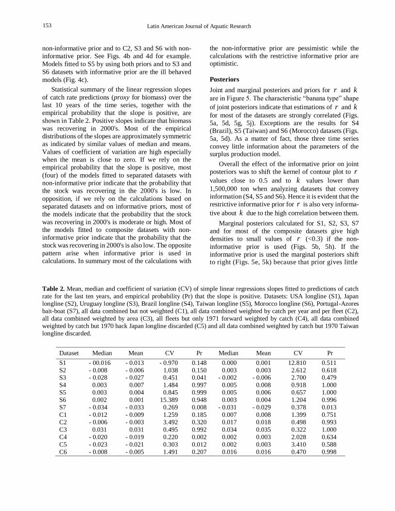
Statistical summary of the linear regression slopes

of catch rate predictions (proxy for biomass) over the

last 10 years of the time series, together with the

empirical probability that the slope is positive, are

shown in Table 2. Positive slopes indicate that biomass

was recovering in 2000's. Most of the empirical

distributions of the slopes are approximately symmetric

as indicated by similar values of median and means.

Values of coefficient of variation are high especially

when the mean is close to zero. If we rely on the

empirical probability that the slope is positive, most

(four) of the models fitted to separated datasets with

non-informative prior indicate that the probability that

the stock was recovering in the 2000's is low. In

opposition, if we rely on the calculations based on

separated datasets and on informative priors, most of

the models indicate that the probability that the stock

was recovering in 2000's is moderate or high. Most of

the models fitted to composite datasets with non-

informative prior indicate that the probability that the

stock was recovering in 2000's is also low. The opposite

pattern arise when informative prior is used in

calculations. In summary most of the calculations with

the non-informative prior are pessimistic while the

calculations with the restrictive informative prior are optimistic.

Posteriors

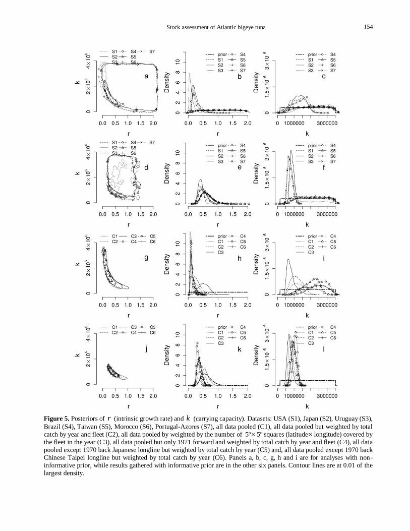
Joint and marginal posteriors and priors for r and k

are in Figure 5. The characteristic “banana type” shape

of joint posteriors indicate that estimations of r and k

for most of the datasets are strongly correlated (Figs.

5a, 5d, 5g, 5j). Exceptions are the results for S4

(Brazil), S5 (Taiwan) and S6 (Morocco) datasets (Figs.

5a, 5d). As a matter of fact, those three time series

convey little information about the parameters of the surplus production model.

Overall the effect of the informative prior on joint

posteriors was to shift the kernel of contour plot to r

values close to 0.5 and to k values lower than

1,500,000 ton when analyzing datasets that convey

information (S4, S5 and S6). Hence it is evident that the

restrictive informative prior for r is also very informa-

tive about k due to the high correlation between them.

Marginal posteriors calculated for S1, S2, S3, S7

and for most of the composite datasets give high

densities to small values of r (<0.3) if the non-

informative prior is used (Figs. 5b, 5h). If the

informative prior is used the marginal posteriors shift to right (Figs. 5e, 5k) because that prior gives little

Table 2. Mean, median and coefficient of variation (CV) of simple linear regressions slopes fitted to predictions of catch

rate for the last ten years, and empirical probability (Pr) that the slope is positive. Datasets: USA longline (S1), Japan

longline (S2), Uruguay longline (S3), Brazil longline (S4), Taiwan longline (S5), Morocco longline (S6), Portugal-Azores

bait-boat (S7), all data combined but not weighted (C1), all data combined weighted by catch per year and per fleet (C2),

all data combined weighted by area (C3), all fleets but only 1971 forward weighted by catch (C4), all data combined

weighted by catch but 1970 back Japan longline discarded (C5) and all data combined weighted by catch but 1970 Taiwan

longline discarded.

Dataset Median Mean CV Pr Median Mean CV Pr

S1 - 00.016 - 0.013 - 0.970 0.148 0.000 0.001 12.810 0.511

S2 - 0.008 - 0.006 1.038 0.150 0.003 0.003 2.612 0.618 S3 - 0.028 - 0.027 0.451 0.041 - 0.002 - 0.006 2.700 0.479

S4 0.003 0.007 1.484 0.997 0.005 0.008 0.918 1.000

S5 0.003 0.004 0.845 0.999 0.005 0.006 0.657 1.000

S6 0.002 0.001 15.389 0.948 0.003 0.004 1.204 0.996

S7 - 0.034 - 0.033 0.269 0.008 - 0.031 - 0.029 0.378 0.013

C1 - 0.012 - 0.009 1.259 0.185 0.007 0.008 1.399 0.751

C2 - 0.006 - 0.003 3.492 0.320 0.017 0.018 0.498 0.993

C3 0.031 0.031 0.495 0.992 0.034 0.035 0.322 1.000

C4 - 0.020 - 0.019 0.220 0.002 0.002 0.003 2.028 0.634

C5 - 0.023 - 0.021 0.303 0.012 0.002 0.003 3.410 0.588

C6 - 0.008 - 0.005 1.491 0.207 0.016 0.016 0.470 0.998

153


Figure 5. Posteriors of r (intrinsic growth rate) and k (carrying capacity). Datasets: USA (S1), Japan (S2), Uruguay (S3),

Brazil (S4), Taiwan (S5), Morocco (S6), Portugal-Azores (S7), all data pooled (C1), all data pooled but weighted by total

catch by year and fleet (C2), all data pooled by weighted by the number of 5º5º squares (latitude longitude) covered by

the fleet in the year (C3), all data pooled but only 1971 forward and weighted by total catch by year and fleet (C4), all data

pooled except 1970 back Japanese longline but weighted by total catch by year (C5) and, all data pooled except 1970 back

Chinese Taipei longline but weighted by total catch by year (C6). Panels a, b, c, g, h and i are for analyses with non-

informative prior, while results gathered with informative prior are in the other six panels. Contour lines are at 0.01 of the

largest density.

154


weight to low values of r (<0.25). Posteriors of r for

S4, S5 and S6 datasets are strongly affected by the

informative prior. Because those three datasets do not

convey information about r , if the informative prior is

used, the posteriors are equal to the prior, but they are flat if the non-informative prior is used.

All separated datasets convey little information

about k, hence the precisions of the marginal posteriors

are low if the non-informative set of priors are used in

the calculations (Fig. 5c). As a matter of fact S4, S5 and

S6 convey no information about k and the posteriors

are flat and truncated in the right tail by the prior (Figs.

5c, 5f). Posteriors of k as calculated for the datasets

S1, S2, S3 and S7 are much more precise when

informative priors are used (Fig. 5f). Densities are high for values close to 800,000 ton.

Composite datasets convey information about k

but the calculated posteriors are contradictory. For

example, if the non-informative priors are used the

mode of the posterior for C3 dataset (all data weighted

by area) is close to 600,000 ton, while the mode of the

posterior for C4 (only 1971 forward data weighted by

catch) is close to 3,000,000 ton (Fig. 5i). The modes of

the more precise posteriors as calculated with

informative prior are close to 1,000,000 ton for all the

composite datasets (Fig. 5l).

Posteriors for q are not shown to not clutter.

Nevertheless most of the comments above concerning

estimations and effects of priors on the posteriors of r

and k are also valid for posteriors of q. In summary, all

marginal posteriors were unimodal and the precision of

the calculated posteriors with informative prior are

usually higher than those calculated with the non-

informative prior.

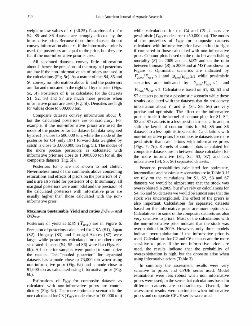
Maximum Sustainable Yield and ratios F/FMSY and

B/BMSY

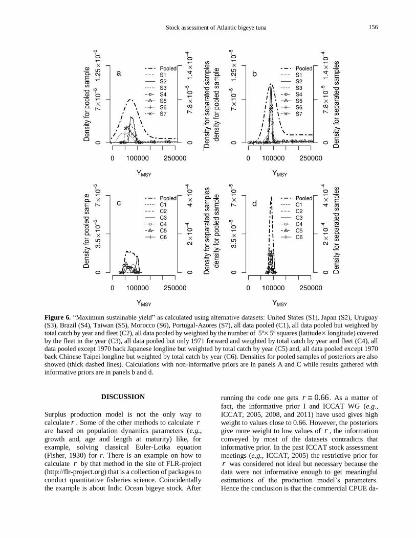
Posteriors of yield at MSY ( MSYY ) are in Figure 6.

Precision of posteriors calculated for USA (S1), Japan

(S2), Uruguay (S3) and Portugal-Azores (S7) were

large, while posteriors calculated for the other three

separated datasets (S4, S5 and S6) were flat (Figs. 6a-

6b). All posterior samples were pooled to summarize

the results. The “pooled posterior” for separated

datasets has a mode close to 73,000 ton when using

non-informative prior (Fig. 6a) and a mode close to

91,000 ton as calculated using informative prior (Fig. 6b).

Estimations of YMSY for composite datasets as calculated with non-informative priors are contra-

dictory (Fig. 6c). The more optimistic scenario is the

one calculated for C3 (YMSY mode close to 100,000 ton)

while calculations for the C4 and C5 datasets are

pessimistic (YMSY mode close to 50,000 ton). The modes

of the posteriors of YMSY for composite datasets

calculated with informative prior have shifted to right

if compared to those calculated with non-informative

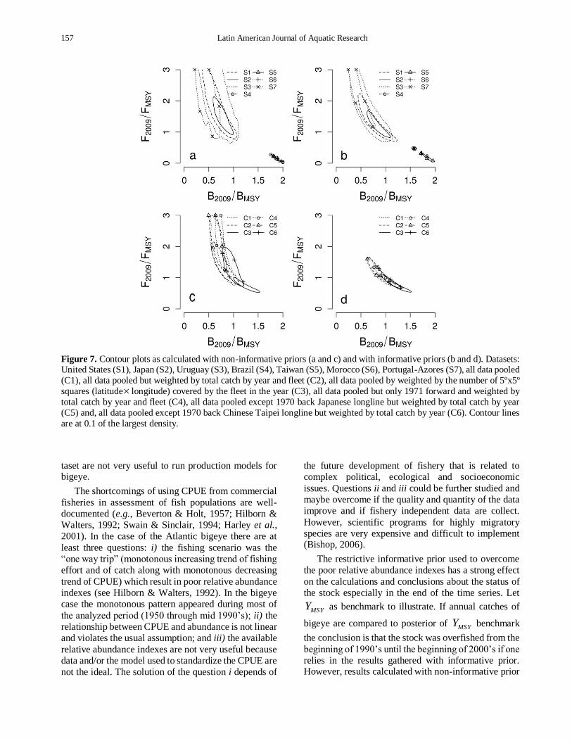
prior. Contour plots based on the ratio between fishing

mortality (F) in 2009 and at MSY and on the ratio

between biomass (B) in 2009 and at MSY are shown in

Figure 7. Optimistic scenarios are indicated by

12009 MSYFF and 12009 MSYBB while pessimistic

scenarios are indicated by 12009 MSYFF and

12009 MSYBB . Calculations based on S1, S2, S3 and

S7 datasets point for a pessimistic scenario while those

results calculated with the datasets that do not convey

information about r and k (S4, S5, S6) are very

precise and optimistic. The effect of the informative

prior is to shift the kernel of contour plots for S1, S2,

S3 and S7 datasets to a less pessimistic scenario and, to

shift the kernel of contour plots for S4, S5 and S6

datasets to a less optimistic scenario. Calculations with

non-informative priors for composite datasets are more

pessimistic than calculations with informative priors

(Figs. 7c-7d). Kernels of contour plots calculated for

composite datasets are in between those calculated for

the more informative (S1, S2, S3, S7) and less informative (S4, S5, S6) separated datasets.

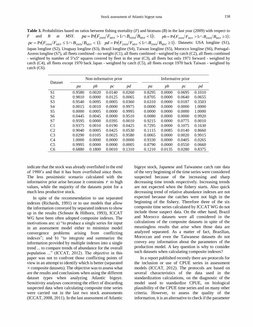
Posterior probabilities calculated for optimistic,

intermediate and pessimistic scenarios are in Table 3. If

we rely on the calculations for S1, S2, S3 and S7

datasets we would be almost sure that the stock was

overexploited in 2009, but if we rely on calculations for

S4, S5 and S6 datasets we would be almost sure that the

stock was underexploited. The effect of the priors is

also important. Calculations for separated datasets

based on the informative prior are more optimistic.

Calculations for some of the composite datasets are also

very sensitive to priors. Most of the calculations with

the non-informative prior indicate that the stock was

overexploited in 2009. However, only three models

indicate overexploitation if the informative prior is

used. Calculations for C2 and C6 datasets are the more

sensitive to prior. If the non-informative priors are

used, the results indicate that the probability of

overexploitation is high, but the opposite arise when

using informative priors (Table 3).

In summary the assessment results were very

sensitive to priors and CPUE series used. Model

estimations were less robust when non informative

priors were used; in the sense that calculations based in

different datasets are contradictory. Overall, the

assessment results were optimistic when informative

priors and composite CPUE series were used.

155


Figure 6. “Maximum sustainable yield” as calculated using alternative datasets: United States (S1), Japan (S2), Uruguay

(S3), Brazil (S4), Taiwan (S5), Morocco (S6), Portugal-Azores (S7), all data pooled (C1), all data pooled but weighted by

total catch by year and fleet (C2), all data pooled by weighted by the number of 5º5º squares (latitude longitude) covered

by the fleet in the year (C3), all data pooled but only 1971 forward and weighted by total catch by year and fleet (C4), all

data pooled except 1970 back Japanese longline but weighted by total catch by year (C5) and, all data pooled except 1970

back Chinese Taipei longline but weighted by total catch by year (C6). Densities for pooled samples of posteriors are also

showed (thick dashed lines). Calculations with non-informative priors are in panels A and C while results gathered with

informative priors are in panels b and d.

DISCUSSION

Surplus production model is not the only way to

calculate r . Some of the other methods to calculate r

are based on population dynamics parameters (e.g.,

growth and, age and length at maturity) like, for

example, solving classical Euler-Lotka equation

(Fisher, 1930) for r. There is an example on how to

calculate r by that method in the site of FLR-project (http://flr-project.org) that is a collection of packages to

conduct quantitative fisheries science. Coincidentally

the example is about Indic Ocean bigeye stock. After

running the code one gets 66.0r . As a matter of

fact, the informative prior I and ICCAT WG (e.g.,

ICCAT, 2005, 2008, and 2011) have used gives high

weight to values close to 0.66. However, the posteriors

give more weight to low values of r , the information

conveyed by most of the datasets contradicts that

informative prior. In the past ICCAT stock assessment

meetings (e.g., ICCAT, 2005) the restrictive prior for

r was considered not ideal but necessary because the data were not informative enough to get meaningful

estimations of the production model’s parameters.

Hence the conclusion is that the commercial CPUE da-

156


Figure 7. Contour plots as calculated with non-informative priors (a and c) and with informative priors (b and d). Datasets: United States (S1), Japan (S2), Uruguay (S3), Brazil (S4), Taiwan (S5), Morocco (S6), Portugal-Azores (S7), all data pooled

(C1), all data pooled but weighted by total catch by year and fleet (C2), all data pooled by weighted by the number of 5ºx5º

squares (latitude longitude) covered by the fleet in the year (C3), all data pooled but only 1971 forward and weighted by

total catch by year and fleet (C4), all data pooled except 1970 back Japanese longline but weighted by total catch by year

(C5) and, all data pooled except 1970 back Chinese Taipei longline but weighted by total catch by year (C6). Contour lines

are at 0.1 of the largest density.

taset are not very useful to run production models for bigeye.

The shortcomings of using CPUE from commercial

fisheries in assessment of fish populations are well-

documented (e.g., Beverton & Holt, 1957; Hilborn &

Walters, 1992; Swain & Sinclair, 1994; Harley et al.,

2001). In the case of the Atlantic bigeye there are at

least three questions: i) the fishing scenario was the

“one way trip” (monotonous increasing trend of fishing

effort and of catch along with monotonous decreasing

trend of CPUE) which result in poor relative abundance

indexes (see Hilborn & Walters, 1992). In the bigeye

case the monotonous pattern appeared during most of

the analyzed period (1950 through mid 1990’s); ii) the

relationship between CPUE and abundance is not linear

and violates the usual assumption; and iii) the available

relative abundance indexes are not very useful because

data and/or the model used to standardize the CPUE are

not the ideal. The solution of the question i depends of

the future development of fishery that is related to

complex political, ecological and socioeconomic

issues. Questions ii and iii could be further studied and

maybe overcome if the quality and quantity of the data

improve and if fishery independent data are collect.

However, scientific programs for highly migratory

species are very expensive and difficult to implement (Bishop, 2006).

The restrictive informative prior used to overcome

the poor relative abundance indexes has a strong effect

on the calculations and conclusions about the status of

the stock especially in the end of the time series. Let

MSYY as benchmark to illustrate. If annual catches of

bigeye are compared to posterior of MSYY benchmark

the conclusion is that the stock was overfished from the

beginning of 1990’s until the beginning of 2000’s if one

relies in the results gathered with informative prior. However, results calculated with non-informative prior

157


Table 3. Probabilities based on ratios between fishing mortality (F) and biomass (B) in the last year (2009) with respect to

F and B at MSY. 11Pr 20092009 MSYMSY BBFFpa ; 11Pr 20092009 MSYMSY BBFFpb ;

11Pr 20092009 MSYMSY BBFFpc ; 11Pr 20092009 MSYMSY BBFFpd . Datasets: USA longline (S1),

Japan longline (S2), Uruguay longline (S3), Brazil longline (S4), Taiwan longline (S5), Morocco longline (S6), Portugal-

Azores longline (S7), all fleets combined - no weight (C1), all fleets combined - weighted by catch (C2), all fleets combined

- weighted by number of 5ºx5º squares covered by fleet in the year (C3), all fleets but only 1971 forward - weighted by

catch (C4), all fleets except 1970 back Japan - weighted by catch (C5), all fleets except 1970 back Taiwan - weighted by

catch (C6).

Dataset Non-informative prior Informative prior

pa pb pc pd pa pb pc pd

S1 0.9580 0.0020 0.0140 0.0260 0.8295 0.0000 0.0695 0.1010 S2 0.9810 0.0000 0.0125 0.0065 0.8705 0.0000 0.0640 0.0655

S3 0.9540 0.0095 0.0005 0.0360 0.6310 0.0000 0.0187 0.3503

S4 0.0015 0.0010 0.0000 0.9975 0.0000 0.0000 0.0000 1.0000

S5 0.0000 0.0005 0.0000 0.9995 0.0000 0.0000 0.0000 1.0000

S6 0.0445 0.0045 0.0000 0.9510 0.0080 0.0000 0.0000 0.9920

S7 0.9595 0.0000 0.0395 0.0010 0.9215 0.0000 0.0775 0.0010

C1 0.9375 0.0010 0.0190 0.0425 0.7295 0.0000 0.1075 0.1630

C2 0.9040 0.0005 0.0425 0.0530 0.1115 0.0085 0.0140 0.8660

C3 0.0290 0.0105 0.0025 0.9580 0.0065 0.0000 0.0020 0.9915

C4 1.0000 0.0000 0.0000 0.0000 0.9330 0.0000 0.0405 0.0265

C5 0.9995 0.0000 0.0000 0.0005 0.8790 0.0000 0.0550 0.0660 C6 0.6880 0.1800 0.0010 0.1310 0.1210 0.0135 0.0280 0.8375

indicate that the stock was already overfished in the end

of 1980’s and that it has been overfished since them.

The less pessimistic scenario calculated with the

informative prior arise because it constrains r to high

values, while the majority of the datasets point for a

much less productive stock.

In spite of the recommendation to use separated

indexes (Richards, 1991) or to use models that allow

the information conveyed by separated indexes to show

up in the results (Schnute & Hilborn, 1993), ICCAT

WG have been often adopted composite indexes. The

motivations are: a) “to produce a single series for input

in an assessment model either to minimize model

convergence problems arising from conflicting

indexes”; and b) “to integrate and summarize the

information provided by multiple indexes into a single

trend ... to compare trends of abundance for the overall

population ...” (ICCAT, 2012). The objective in this

paper was not to confront those conflicting points of

view in an attempt to identify which is better (separated

composite datasets). The objective was to assess what

are the results and conclusions when using the different

dataset types when analyzing Atlantic bigeye.

Sensitivity analyses concerning the effect of discarding suspected data when calculating composite time series

were carried out in the last two stock assessments

(ICCAT, 2008, 2011). In the last assessment of Atlantic

bigeye stock, Japanese and Taiwanese catch rate data

of the very beginning of the time series were considered

suspected because of the increasing and sharp

decreasing time trends respectively. Increasing trends

are not expected when the fishery starts. Also quick

decreasing trend of relative abundance indexes are not

expected because the catches were not high in the

beginning of the fishery. Therefore three of the six

composite time series calculated by ICCAT WG do not

include those suspect data. On the other hand, Brazil

and Morocco datasets were all considered in the

calculations of the composite datasets in spite of the

meaningless results that arise when those data are

analyzed separated. As a matter of fact, Brazilian,

Moroccan and even the Taiwanese datasets do not

convey any information about the parameters of the

production model. A key question is why to consider such datasets when calculating composite indexes?

In a report published recently there are protocols for

the inclusion or use of CPUE series in assessment

models (ICCAT, 2012). The protocols are based on

several characteristics of the data used in the

standardization calculations, on the diagnostic of the

model used to standardize CPUE, on biological plausibility of the CPUE time series and on many other

criteria. However, to assess the quality of the

information, it is an alternative to check if the parameter

158


calculations based on the datasets are meaningful. If

this criterion is adopted, Brazilian, Moroccan and

Taiwanese datasets should not be considered in the

calculations of the composite indexes. If the results of

the stock assessment gathered with the different

composite datasets point for the same stock status, the

discussion about weights and procedures used to

calculate composite datasets are of secondary

importance. However this is not the case for bigeye.

Posteriors were more affected by the choice about the

procedure used to calculate the composite datasets

(e.g., weighting by catch or by area) than by the choice

about discarding suspected data of the beginning of the

time series. While the choice of the weights is of major

importance it is usually subjective. Alternative

approaches to calculate composite indexes are in

ICCAT (2012) but there is not guidance to assess how

suitable are a given weighting criterion. Uncertainty

that arise in the posteriors when analyzing the original

separated dataset is not properly depicted in the

calculations for the composite datasets. One might keep

in mind that because the composite datasets are

“averages”, the high precision of the calculations is

artificial. Therefore the results of stock assessment

based on composite datasets should be carefully

considered whenever they are used as guidelines for

management decisions and recommendations.

If one rely on MSYY benchmark, most of the results

indicate that probably the Atlantic bigeye stock have

been overfished during 1990’s. Also, the calculations

of probability that 12009 MSYFF and that

12009 MSYBB indicate that bigeye stock was still

overfished in the end of 2000’s. Nevertheless, there is

doubt about if the stock has begun to recover since the

beginning of 2000’s. If we rely on those separated

datasets that convey some information (S1, S2, S3 and

S7) or, in the results obtained for composite datasets

with non-informative priors, the answer is no, probably

the stock was not recovering in the 2000’s. If we rely

on the results gathered with composite datasets and

informative prior, the opposite answer arises. In

summary the diagnostic about the time trend of the

abundance of Atlantic bigeye depends on the dataset and on the prior considered.

Finally it is important to recognize that the analysis

showed in this paper is just one among several possible

approaches. The model used here is a simple single

species one, and the usefulness of such models as tool

for stock assessment and management is debatable

(Hollowed et al., 2000; Prager, 2002, 2003; Maunder,

2003; Walters et al., 2005). Therefore, this paper might

not be the only document considered when assessing

the Atlantic bigeye stock. Instead the paper was wrote

to show how informative are the available datasets to

run production models and how important are the issues

regarding the alternatives composite versus separated

datasets and non-informative versus informative priors for Atlantic bigeye tuna.

CONCLUSIONS

Relative abundance indexes for bigeye as calculated

using commercial data are not very informative about

parameters of surplus production models; hence

scientific programs to obtain fishery independent

relative abundance indexes for Atlantic bigeye are

encouraged. Most of the results of the production

models indicate that bigeye stock was overexploited in

1990's. However the conclusion about the possibility

that the stock was recovering in 2000’s depends on the dataset and on the prior.

AKNONWLEDGMENTS

I am grateful to two anonymous reviewers for the valuable comments and constructive criticisms.

REFERENCES

Andrade, H.A. & P.G. Kinas. 2007. Decision analysis on

the introduction of new fishing fleet for skipjack tuna

in the Southwest Atlantic. PanamJAS, 2(2): 131-148.

Berger, J.O. 1985. Statistical decision theory and Bayesian

analysis. Springer-Verlag, New York, 617 pp.

Beverton, R.J. & S.J. Holt. 1957. On the dynamics of

exploited fish populations. Fish. Invest. Ser. II. Mar.

Fish. G.B. Minist. Agric. Fish. Food, 19: 533 pp.

Bishop, J. 2006. Standardizing fishery-dependent catch

and effort data in complex fisheries with technology

change. Rev. Fish Biol. Fish., 16: 21-38.

Fisher, R. 1930. The genetical theory of natural selection.

Clarendon Press, Oxford, 272 pp.

Gelman, A., J.B. Carlin, H.S. Stern & D.B. Rubin. 1995.

Bayesian data analysis. Chapman & Hall, London, 526

pp.

Givens, G.H. 1993. Contribution to discussion on the

meeting on the Gibbs sampler and other Markov chain

Monte Carlo methods. J. R. Stat. Soc., B55: 75-76.

Graham, M. 1935. Modern theory of exploiting a fishery

and applications to North Sea trawling. J. Cons. Int.

Explor. Mer, 10: 264-274.

Harley, S.J., R.A. Myers & A. Dunn. 2001. Is catch-per-

unit-effort proportional to abundance? Can. J. Fish.

Aquat. Sci., 58: 1760-1772.

159


Hilborn, R. & C.J. Walters. 1992. Quantitative fisheries

stock assessment. Chapman & Hall, New York, 570 pp.

Hollowed, A.B., N. Bax., R. Beamish, J. Collie, M.

Fogarty, P. Livingston, J. Pope & J.C. Rice. 2000. Are

multispecies models an improvement on single-

species models for measuring fishing impacts on

marine ecosystems? ICES J. Mar. Sci., 57: 707-719.

International Commission for Conservation of Atlantic

Tunas (ICCAT). 2005. Report of the 2004 ICCAT

bigeye tuna stock assessment session. Collect. Vol.

Sci. Pap., 58(1): 1-110.




Sci. Pap., 62(1): 97-239.


Tunas (ICCAT). 2010. Report for biennial period,

2008-09. Part II (2009), Vol. 2, 344 pp.




Sci. Pap., 66(1): 1-186.


Tunas (ICCAT). 2012. Report of the 2012 meeting of the ICCAT Working Group on stock assessment

methods, 23 pp.

Kinas, P.G. 1996. Bayesian fishery stock assessment and

decision making using adaptive importance sampling.

Can. J. Fish. Aquat. Sci., 53: 414-423.

Ludwig, D. & C.J. Walters. 1985. Are age-structured

models appropriate for catch-effort data? Can. J. Fish.

Aquat. Sci., 42: 1066-1072.

Maunder, M.N. 2003. Letter to the editor. Fish. Res., 61:

145-149.

Maunder, M.N. & A.E. Punt. 2004. Standardizing catch

and effort data: a review of recent approaches. Fish. Res., 70: 141-159.

McAllister, M.K. & J.N. Ianelli. 1997. Bayesian stock

assessment using catch-agedata and the

sampling/importance resampling algorithm. Can. J.

Fish. Aquat. Sci., 54: 284-300.

McAllister, M.K. & G.P. Kirkwood. 1998. Bayesian stock

assessment: a review and example application using

the logistic model. ICES J. Mar. Sci., 55: 1031-1060.

Methot, R.D. 1990. Synthesis model: an adaptable

framework for analysis of diverse stock assessment

data. Int. N. Pac. Fish. Comm. Bull., 50: 259-277.

Meyer, R. & R.B. Millar. 1999a. Bayesian stock

assessment using a state-space implementation of the

delay difference model. Can. J. Fish. Aquat. Sci., 56:

37-52.

Meyer, R. & R.B. Millar. 1999b. BUGS in Bayesian stock

assessments. Can. J. Fish. Aquat. Sci., 56: 1078-1086.

Millar, R.B. 2002. Reference priors for Bayesian fisheries

models. Can. J. Fish. Aquat. Sci., 59: 1492-1502.

Miyake, M.P., N. Miyabe & H. Nakano. 2004. Historical

trends of tuna catch in the world. FAO Fish. Tech.

Pap., 467: 83 pp.

Newton, M.A. & A.E. Raftery. 1994. Approximate

Bayesian inference with the weighted likelihood

bootstrap. J. R. Stat. Soc., B56: 3-48.

Oh, M.S. & J.O. Berger. 1992. Adaptive importance

sampling in Monte Carlo integration. J. Statist.

Comput. Simul., 41: 143-168.

Prager, M.H. 2002. Comparison of logistic and

generalized surplus-production models applied to

swordfish, Xiphias gladius, in the North Atlantic Ocean. Fish. Res., 58: 41-57.

Prager, M.H. 2003. Reply to the letter to the editor. Fish.

Res., 61: 151-154.

Punt, A.E. 1990. Is kB 1 an appropriate assumption

when applying and observation error production-

model estimator to catch-effort data? S. Afr. J. Mar. Sci., 9: 249-259.

Punt, A.E. & R. Hilborn. 1997. Fisheries stock assessment

and decision analysis: the Bayesian approach. Rev.

Fish Biol. Fish., 7: 35-63.

Raftery, A.E., G.H. Givens & J.E. Zeh. 1995. Inference

from a deterministic population dynamics model for

bowhead whales. J. Am. Stat. Assoc., 90: 402-416.

Richards, L.J. 1991. Use of contradictory data sources in

stock assessment. Fish. Res., 11: 225-238.

Schaefer, M.B. 1954. Some aspects of dynamics of

populations important to management of commercial

marine fisheries. Int. Am. Trop. Tuna Comm. Bull., 1: 25-56.

Schnute, J.T. & R. Hilborn. 1993. Analysis of

contradictory data sources in fish stock assessment.

Can. J. Fish. Aquat. Sci., 50: 1916-1923.

Silverman, B.W. 1986. Density estimation for statistics

and data analysis. Chapman & Hall, Boca Raton, 175

pp.

Smith, A.F.M. 1991. Bayesian computational methods.

Philos. T. R. Soc. Lond., A337: 369-386.

Smith, A.F.M. & A.E. Gelfand. 1992. Bayesian statistics

without tears: a sampling-resampling perspective. Am. Statist., 46(2): 84-88.

Swain, D.P. & A.F. Sinclair. 1994. Fish distribution and

catchability: what is the appropriate measure of

distribution? Can. J. Fish. Aquat. Sci., 51: 1046-1054.

Walters, C.J., V. Christensen, S. J. Martell & J. F. Kitchell.

2005. Possible ecosystem impacts of applying MSY

policies from single-species assessment. ICES J. Mar.

Sci., 62: 558-568.

West, M. 1992. Modelling with mixtures. In: J.M.

Bernardo, J.O. Berger, A.P. Dawid & A.F.M. Smith

160


(eds.). Bayesian statistics 4. Oxford University Press,

Oxford, pp. 503-524.

Received: 28 June 2013; Accepted: 14 October 2014

West, M. 1993. Approximating posterior distributions by

mixtures. J. R. Stat. Soc., B55: 409-422.

Van Dijk, H.K. & T. Kloek. 1983. Monte Carlo analysis

of skew posterior distributions: an illustrative

economic example. Statistician, 32: 216-233.

161

sensitivity analysis of catch-per-unit-effort of atlantic bigeye tuna ... · palabras clave:...

Documents