Sensitivity of Markov chains for wirelessprotocols

Problem presented by

Keith Briggs

BT

Problem statement

Many wireless network protocols lead to Markov chain models with atransition matrix P (α) depending on some parameters α. From this thesteady state distribution z(α) can be computed, and from this the finaldesired quantities q(α), which might be for example the throughput of theprotocol. To optimise q efficiently we wish to have its gradient with respectto α. There are formulas for dz/dα in terms of (I − P )# but what are thebest numerical techniques for obtaining the derivatives, and are they stable ?Can we also obtain the derivatives of the mixing time and mean hitting timesH ?

The Study Group showed that in general the techniques of sparse linearalgebra and preconditioning should be used for calculating z, H and theirderivatives, and sparse eigenvalue software for mixing times, rather than anynumerical computation of (I−P )#. For a particular example of interest (theBianchi chain) these methods were applied and shown to be very efficient, andthe same can be expected for any chain with a similar “escalator” structure.

Study Group contributors

David Allwright (Smith Institute)Paul Dellar (Imperial College)

Jens Gravesen (Technical University of Denmark)Jan Van Lent (University of Bath)Rob Scheichl (University of Bath)

Maxim Zyskin (University of Bristol)

Report prepared by

David Allwright (Smith Institute)Paul Dellar (Imperial College)

E-1

1 Introduction

Network communication protocols such as the IEEE 802.11 wireless protocol arecurrently best modelled as Markov chains. In these situations we have some protocolparameters α, and a transition matrix P (α) from which we can compute the steady state(equilibrium) distribution z(α) and hence final desired quantities q(α), which might befor example the throughput of the protocol. Typically the chain will have thousands ofstates, and a particular example of interest is the Bianchi chain defined later. Generallywe want to optimise q, perhaps subject to some constraints that also depend on theMarkov chain. To do this efficiently we need the gradient of q with respect to α, andtherefore need the gradient of z and other properties of the chain with respect to α. Thematrix formulas available for this (e.g. in [12] and [4]) involve the so-called fundamentalmatrix (I−P )# = (I−P +1zT)−1−1zT, where z is the equilibrium state and 1 a vectorof 1s. Then dzT/dα = zT (dP/dα) (I−P )#, but is this the best numerical method, and isit stable ? Are there approximate gradients available which are faster and still sufficientlyaccurate ? In some cases BT would like to do the whole calculation in computer algebra,and get a series expansion of the equilibrium z with respect to a parameter in P . Inaddition to the steady state z, the same questions arise for the mixing time and the meanhitting times. The mixing time can here be thought of as (| log |λ2||)−1 or 1/(1 − |λ2|)where |λ2| is the second largest absolute value of the eigenvalues of P (although Example26 of [1] shows this may not always have such a close link to mixing as is sometimesclaimed).

Two qualitative features that were brought to the Study Group’s attention were:

• the transition matrix P is large, but sparse.

• the systems of linear equations to be solved are generally singular and need someadditional normalisation condition, such as is provided by using the fundamentalmatrix (I − P )#.

We also note a third highly important property regarding applications of numerical linearalgebra:

• the transition matrix P is asymmetric.

A realistic dimension for the matrix P in the Bianchi model [3] described below is8064 × 8064, but on average there are only a few nonzero entries per column. Merelystoring such a large matrix in dense form would require nearly 0.5 GBytes using 64-bitfloating point numbers, and computing its LU factorisation takes around 80 seconds ona modern microprocessor. It is thus highly desirable to employ specialised algorithms forsparse matrices. These algorithms are generally divided between those only applicable tosymmetric matrices, the most prominent being the conjugate-gradient (CG) algorithmfor solving linear equations (e.g. [8]), and those applicable to general matrices. A similardivision is present in the literature on numerical eigenvalue problems.

E-2

In the problems encountered at the Study Group, the singular matrices of dimension nhad rank n− 1. We restored each matrix to full rank by replacing one row or column toimpose a suitable normalisation condition: examples of how this was done will be givenin Section 3.1.

We shall also show how the derivatives of the steady state and eigenvalues with respectto the parameters in P may be computed in terms of the corresponding derivatives of P .These computations may be formulated using matrix perturbation theory, as commonlymet for Hermitian matrices in the context of quantum mechanics.

This study is motivated by the Bianchi model [3] for which some quantities of interest,notably the equilibrium population, may be written down explicitly. However, thenumerical techniques employed should be applicable much more widely. The key featurethat we exploit is the presence of “escalator” structures in the transition matrix.Escalators correspond to deterministic increments of a backoff time counter in thecommunication protocol. In linear algebra terms, the escalators contribute transposedJordan blocks to the transition matrix. The spectra of the transition matrices shownbelow in Figure 5 are typical of the behaviour of Jordan blocks under the addition ofsmall perturbations. Each Jordan block has a single degenerate eigenvalue that splitsinto a circular pattern when perturbed. These spectra are highly undesirable for efficientperformance of iterative methods like GMRES [14], but the lower triangular part of thematrix (or even just the bidiagonal matrix of the unperturbed Jordan block) makes ahighly effective preconditioner. A concrete example is given below in Section 4.3.

1.1 The Bianchi chain

A particular example of interest is the Bianchi model of an RTS/CTS WAP protocol.This has parameters

W = minimum congestion window (1)

m = value such that 2mW is the maximum congestion window (2)

p = packet loss probability, computed from the number of users. (3)

The states of the system form m + 1 downward-going escalators E0, E1, . . . , Em ofheights W0, W1, . . . , Wm where Wi = 2iW . The states are labelled by (i, k) wherei ∈ {0, 1, . . . , m} labels the backoff stage (i.e. which escalator), and k ∈ {0, 1, . . . , Wi−1}is the backoff time counter (height on that escalator). The dynamics may be summarisedby the following rules.

• From (i, k) with k ≥ 1, move with probability one to state (i, k−1), one step downEi.

• From (i, 0) (the bottom of Ei) jump with probability 1 − p to a random point onescalator E0.

• From (i, 0) jump with probability p to a random point on escalator Emin(i+1,m).

E-3

In formulae,

p(i, k; i, k − 1) = 1 for each i and for 1 ≤ k ≤ Wi − 1, (4)

p(i, 0; 0, k) =1 − p

W0

for each i and for 0 ≤ k ≤ W0 − 1, (5)

p(i, 0; i + 1, k) =p

Wi+1

for 0 ≤ i ≤ m − 1 and for 0 ≤ k ≤ Wi+1 − 1, (6)

p(m, 0; m, k) =p

Wm

for 0 ≤ k ≤ Wm − 1, (7)

where we use p(i, k; j, l) to denote the 1-step transition probability from (i, k) to (j, l).We can perhaps picture the state as a boy playing on this set of downwards-movingescalators, making random jumps according to these rules when he reaches the bottomof an escalator, but strictly obeying a sign that says “No jumping on the escalators”.The system is represented schematically in the (i, k)-plane in Figure 1.

p

1 − p 1 − p 1 − p

pp

p

1 − p

(0, 0) (1, 0)

(m, Wm − 1)

etc.

etc.

{{ { {

(m − 1, 0) (m, 0)

E1

E0

Em−1

Em

(0, W0 − 1)

(1, W1 − 1)

Figure 1: Schematic diagram of the Bianchi Markov chain. When the systemis on an escalator Ei it descends deterministically at unit rate. When it is atthe bottom of Ei it jumps with probability 1− p to a random state of E0, andwith probability p to a random state of Ei+1 (or Em if i = m).

There are n = (2m+1 − 1)W states, and the case m = 3, W = 32 has 480 states, aboutthe smallest reasonable model. But m might in practice be up to 5, and W up to 128, inwhich case n = 8064. The values of p of interest are generally small, perhaps up to 0.05but with 0.01 as more typical. To arrange the states in a linear order we take first E0

with k increasing, then E1 etc, so (i, k) maps to α = 1 + k + (2i − 1)W with 1 ≤ α ≤ n.

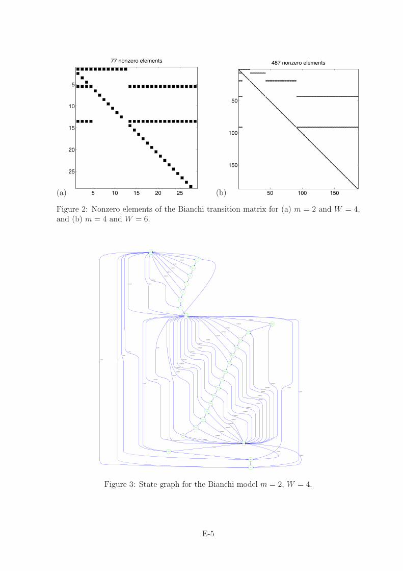
Figure 2 shows the sparsity pattern of the transition matrix for two different choices ofm and W : the black entries are those that are positive, the others are 0. Both choicesgive much smaller matrices than would be realistic. Choosing m = 5 and W = 128 givesan 8064 × 8064 matrix that would be difficult to plot.

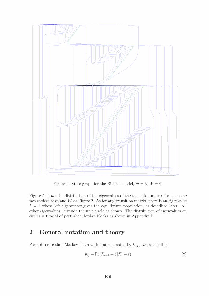
The diagram in Figure 3 shows the transitions for m = 2, W = 4, and Figure 4 is form = 3, W = 6. The “escalators” visible in these graphs and in the sparsity patterndiagrams are a typical structure, whatever the values of W and m.

E-4

(a) 5 10 15 20 25

5

10

15

20

25

77 nonzero elements

(b) 50 100 150

50

100

150

487 nonzero elements

Figure 2: Nonzero elements of the Bianchi transition matrix for (a) m = 2 and W = 4,and (b) m = 4 and W = 6.

0 (0,0) 0.2475

1 (0,1)

0.2475

2 (0,2)

0.2475

3 (0,3)

0.2475

4 (1,0)

0.00125

5 (1,1)

0.00125

6 (1,2)

0.00125

7 (1,3)

0.00125

8 (1,4)

0.00125

9 (1,5)

0.00125

10 (1,6)

0.00125 11 (1,7)

0.00125

1

1

1

0.2475

0.2475

0.2475

0.2475

12 (2,0)

0.000625

13 (2,1)

0.000625

14 (2,2)

0.000625

15 (2,3)

0.000625

16 (2,4)

0.000625

17 (2,5)

0.000625

18 (2,6)

0.000625

19 (2,7)

0.000625

20 (2,8)

0.000625

21 (2,9)

0.000625

22 (2,10)

0.000625

23 (2,11)

0.000625

24 (2,12)

0.000625

25 (2,13)

0.000625

26 (2,14)

0.000625 27 (2,15)

0.000625

1

1

1

1

1

1

1

0.2475

0.2475

0.2475

0.2475

0.000625

0.000625

0.000625

0.000625

0.000625

0.000625

0.000625

0.000625

0.000625

0.000625

0.000625

0.000625

0.000625

0.000625

0.000625

0.000625

1

1

1

1

1

1

1

1

1

1

1

1

1

1

1

Figure 3: State graph for the Bianchi model m = 2, W = 4.

E-5

0 (0,0) 0.165

1 (0,1)

0.165

2 (0,2)

0.165

3 (0,3)

0.165

4 (0,4)

0.165

5 (0,5)

0.165

6 (1,0)

0.000833333

7 (1,1)

0.000833333

8 (1,2)

0.000833333

9 (1,3)

0.000833333

10 (1,4)

0.000833333

11 (1,5)

0.000833333

12 (1,6)

0.000833333

13 (1,7)

0.000833333

14 (1,8)

0.000833333

15 (1,9)

0.000833333

16 (1,10)

0.000833333 17 (1,11)

0.000833333

1

1

1

1

1

0.165

0.165

0.165

0.165

0.165

0.165

18 (2,0)

0.000416667

19 (2,1)

0.000416667

20 (2,2)

0.000416667

21 (2,3)

0.000416667

22 (2,4)

0.000416667

23 (2,5)

0.000416667

24 (2,6)

0.000416667

25 (2,7)

0.000416667

26 (2,8)

0.000416667

27 (2,9)

0.000416667

28 (2,10)

0.000416667

29 (2,11)

0.000416667

30 (2,12)

0.000416667

31 (2,13)

0.000416667

32 (2,14)

0.000416667

33 (2,15)

0.000416667

34 (2,16)

0.000416667

35 (2,17)

0.000416667

36 (2,18)

0.000416667

37 (2,19)

0.000416667

38 (2,20)

0.000416667

39 (2,21)

0.000416667

40 (2,22)

0.000416667 41 (2,23)

0.000416667

1

1

1

1

1

1

1

1

1

1

1

0.165

0.165

0.165

0.165

0.165

0.165

42 (3,0)

0.000208333

43 (3,1)

0.000208333

44 (3,2)

0.000208333

45 (3,3)

0.000208333

46 (3,4)

0.000208333

47 (3,5)

0.000208333

48 (3,6)

0.000208333

49 (3,7)

0.000208333

50 (3,8)

0.000208333

51 (3,9)

0.000208333

52 (3,10)

0.000208333

53 (3,11)

0.000208333

54 (3,12)

0.000208333

55 (3,13)

0.000208333

56 (3,14)

0.000208333

57 (3,15)

0.000208333

58 (3,16)

0.000208333

59 (3,17)

0.000208333

60 (3,18)

0.000208333

61 (3,19)

0.000208333

62 (3,20)

0.000208333

63 (3,21)

0.000208333

64 (3,22)

0.000208333

65 (3,23)

0.000208333

66 (3,24)

0.000208333

67 (3,25)

0.000208333

68 (3,26)

0.000208333

69 (3,27)

0.000208333

70 (3,28)

0.000208333

71 (3,29)

0.000208333

72 (3,30)

0.000208333

73 (3,31)

0.000208333

74 (3,32)

0.000208333

75 (3,33)

0.000208333

76 (3,34)

0.000208333

77 (3,35)

0.000208333

78 (3,36)

0.000208333

79 (3,37)

0.000208333

80 (3,38)

0.000208333

81 (3,39)

0.000208333

82 (3,40)

0.000208333

83 (3,41)

0.000208333

84 (3,42)

0.000208333

85 (3,43)

0.000208333

86 (3,44)

0.000208333

87 (3,45)

0.000208333

88 (3,46)

0.000208333 89 (3,47)

0.000208333

1

1

1

1

1

1

1

1

1

1

1

1

1

1

1

1

1

1

1

1

1

1

1

0.165

0.165

0.165

0.165

0.165

0.165

0.000208333

0.000208333

0.000208333

0.000208333

0.000208333

0.000208333

0.000208333

0.000208333

0.000208333

0.000208333

0.000208333

0.000208333

0.000208333

0.000208333

0.000208333

0.000208333

0.000208333

0.000208333

0.000208333

0.000208333

0.000208333

0.000208333

0.000208333

0.000208333

0.000208333

0.000208333

0.000208333

0.000208333

0.000208333

0.000208333

0.000208333

0.000208333

0.000208333

0.000208333

0.000208333

0.000208333

0.000208333

0.000208333

0.000208333

0.000208333

0.000208333

0.000208333

0.000208333

0.000208333

0.000208333

0.000208333

0.000208333

0.000208333

1

1

1

1

1

1

1

1

1

1

1

1

1

1

1

1

1

1

1

1

1

1

1

1

1

1

1

1

1

1

1

1

1

1

1

1

1

1

1

1

1

1

1

1

1

1

1

Figure 4: State graph for the Bianchi model, m = 3, W = 6.

Figure 5 shows the distribution of the eigenvalues of the transition matrix for the sametwo choices of m and W as Figure 2. As for any transition matrix, there is an eigenvalueλ = 1 whose left eigenvector gives the equilibrium population, as described later. Allother eigenvalues lie inside the unit circle as shown. The distribution of eigenvalues oncircles is typical of perturbed Jordan blocks as shown in Appendix B.

2 General notation and theory

For a discrete-time Markov chain with states denoted by i, j, etc, we shall let

pij = Pr(Xt+1 = j|Xt = i) (8)

E-6

(a) −1 −0.5 0 0.5 1−1

−0.5

0

0.5

1

(b) −1 −0.5 0 0.5 1−1

−0.5

0

0.5

1

Figure 5: Complex eigenvalues of the Bianchi transition matrix for (a) m = 2and W = 4, and (b) m = 4 and W = 6. The unit circle is also shown.

be the 1-step transition probability from i to j, and n be the number of states.1 We alsothink of the states as the vertices of a directed graph, in which there is an edge from ito j if and only if pij > 0, and these are the graphs illustrated in Figures 3 and 4. Weshall assume that the states form a single closed class, i.e. for any states i and j thereis a path from i to j in that graph. We shall also assume that the chain is aperiodic,i.e. it is not possible to partition the states into r ≥ 2 sets A1, A2, . . . , Ar such thatfrom each As you can only get to As+1, and from Ar only to A1. A sufficient conditionfor this is that some pii > 0, or that from some i to some j there are paths of coprimelengths. When these conditions hold, the Markov chain has steady state probabilities

zi = limt→∞

(Pr(Xt = i)) , (9)

and the system is ergodic in the sense that zi is also the long-term proportion of the timethat is spent in state i. Coming now to the matrix formulation, the matrix P = (pij)has P1 = 1 where 1 is a column vector with every entry 1. So λ1 = 1 is an eigenvalueof P , and under the conditions we have assumed, each other eigenvalue lies in |λ| < 1.When the initial probabilities of the system being in state i form a row vector pT

0 , theprobabilities at times 1, 2, . . . are pT

0 P , pT0 P 2 etc. Since zT = (z1, z2, . . . , zn) is the

steady-state distribution, it therefore obeys zTP = zT, so it is the left eigenvector forthe eigenvalue λ1 = 1. The normalisation is fixed by the fact that it is a probabilitydistribution over the states and so

∑zi = zT1 = 1. So from the viewpoint of linear

algebra, zT is determined by zT = zTP together with the condition zT1 = 1 that resolvesthe ambiguity caused by 1 being an eigenvalue of P .

In general if the eigenvalues λi of P are distinct then there will be left eigenvectors zTi

1Of course when we come the the particular example of the Bianchi chain, this i and j will each haveto be replaced by an index α that encodes the pair of indices (i, k) in the Bianchi description.

E-7

and right eigenvectors vi such that

zTi P = λiz

Ti , Pvi = λivi, zT

i vj = δij, (10)

with λ1 = 1, zT1 = zT, v1 = 1, and then

P =n∑

i=1

λivizTi = 1zT +

n∑i=2

λivizTi . (11)

Any initial probability distribution over the states, pT0 , will then have the form

pT0 = zT +

∑ni=2 ξiz

Ti where ξi = pT

0 vi, and after r steps of the Markov process it willbecome

pT0 P r = zT +

n∑i=2

λri ξiz

Ti . (12)

So this tends to zT as r → ∞ and the rate of convergence is governed by the subdominanteigenvalue, i.e. |λ2| if we arrange the eigenvalues by decreasing magnitude,

λ1 = 1 > |λ2| ≥ |λ3| ≥ . . . . (13)

So zT2 is the most persistent (slowest decaying) non-equilibrium behaviour.

In the circumstances we are considering, the mean time to reach state i starting fromany other state j is finite, called the mean hitting time (or just the hitting time) and wedenote it by

Hji = Ex(least t such that Xt = i|X0 = j), (j �= i). (14)

The equations for these come from considering how we get from j to i. We must firsttake 1 step, and then if we have gone to some k �= i the mean number of steps fromthere to i is Hki, so

Hji = 1 +∑k �=i

pjkHki (j �= i). (15)

For fixed i these are n− 1 equations for the n− 1 unknowns Hji and uniquely determinethem. The matrix involved is I − P with row and column i deleted. A further propertyof the hitting times is that

1

zi

= 1 +∑k �=i

pikHki, (16)

since 1/zi is the mean recurrence time for state i, i.e. the mean time between successivevisits to i, which we can write down by the same argument that led to (15). If we definea matrix H0 to be Hij off the diagonal and 0 on the diagonal then these two equationsare combined in

H0 + diag(1/zi) = J + PH0, (17)

where every entry of J is 1: off the diagonal this is (15), and on the diagonal it is (16).Although (17) alone does not determine H0 because I − P is singular, the additionalcondition that H0 has zero diagonal elements resolves that ambiguity.

E-8

2.1 Derivatives with respect to parameters

When the matrix P depends on a vector of parameters α in a differentiable way, we canfind the derivatives of the various properties of the chain by differentiating the definingequations. So from zTP = zT and zT1 = 1 we have(

zT)′

P + zTP ′ =(zT

)′,

(zT

)′1 = 0, (18)

where ′ denotes differentiation with respect to α. So, like zT itself, the vector(zT

)′obeys

a system of linear equations with matrix I − P , together with a condition that resolvesthe ambiguity caused by 1 being an eigenvalue of P .

For differentiating the subdominant eigenvalue λ2, we deal first with the case where λ2 isreal with |λ2| > |λ3|. Then λ2 is an isolated eigenvalue so its left and right eigenvectorsare well-defined and from differentiating the conditions (10) for i = 2 we find that

λ′2 = zT

2 P ′v2. (19)

Equally, if λ2 and λ3 are a complex conjugate pair, with |λ2| = |λ3| > |λ4| then λ2 isisolated and the same result holds, and of course, zT

3 , v3 and λ′3 are just the conjugates of

zT2 , v2 and λ′

2. However, when λ2 is real with |λ2| = |λ3| then there is generally a failureof differentiability. Either λ2 = λ3 in which case the eigenvectors are either not definedor not unique and perturbing P by O(ε) splits the eigenvalues by O(

√ε). Or λ2 �= λ3 in

which case even though the eigenvalues of P vary continuously there is a discontinuousswitch in which of them is subdominant. The same kind of failure of differentiabilitywill happen when λ2 is complex and |λ2| = |λ4|. These cases are not generic as far asP is concerned. However, when one tries to solve an optimisation problem where theobjective function or constraints may involve λ2, then this kind of difficulty can easilyarise because the optimum may well be at a point of non-differentiability of |λ2|. Forinstance if one tries to minimise M = |λ2| subject to some constraints then one can easilyenvisage this optimum occurring for a configuration where P has several eigenvalues onthe circle |λ| = M , but where any feasible perturbation causes some of those eigenvaluesto move into |λ| > M . So the fact that |λ2| is not everywhere differentiable could be ofmore importance than its non-genericity might suggest.

To differentiate the hitting times, we differentiate (17) and see

H ′0 − diag(z′i/z

2i ) = P ′H0 + PH ′

0, (20)

so again H ′0 obeys a system of linear equations with matrix I−P and with the condition

of zero diagonal elements to resolve the ambiguity caused by 1 being an eigenvalue of P .

Whether these equations are solved analytically or numerically, these formulae are thekey to calculating the derivatives.

3 Numerical methods

As explained in the introduction, our aim here is to describe numerical methods thatwill be effective for this kind of problem in general, with a large sparse transition matrix

E-9

P having an escalator structure. The particular illustrations will use the Bianchi chainas the example.

3.1 Equilibrium population

The equilibrium population, zT1 in our notation, is given by

zT1 (I − P ) = 0 , (21)

and to define a unique solution we impose the condition zT1 1 = 1 that makes zT

1 anormalised probability distribution.

When the states of the Markov chain form a single closed class, the matrix I − P isrank-deficient by 1, and we found experimentally that replacing the leftmost column ofthe matrix by a column of ones (1, . . . , 1)T created a matrix with full rank. We chose theleftmost column so that this dense column lies in the lower triangular part of the matrix.This is convenient when using the lower triangular part of the matrix as a preconditionerfor iterative methods, as in Section 4.3 below, but in principle any other column couldbe chosen. One could also add 1 to each entry in the original column of I −P instead ofreplacing the existing entries with 1s. The resulting linear system, written in partitionedform, is

zT1

⎛⎜⎝1

... [I − P ]2...n

1

⎞⎟⎠ = (1, 0, . . . , 0), (22)

where [I − P ]2...n denotes columns 2 to n of the n × n matrix I − P . The transpose ofequation (22) may be treated using numerical methods for solving systems of full rankin the standard form Ax = b, as described in Section 4 below.

An alternative approach to finding eigenvectors is to solve the obvious (notionallysingular) linear system instead of changing one row or column to impose a normalisationcondition. There are matrices where the “eigenvector” computed by changing a rowor column varies wildly depending upon precisely which row or column is chosen. (Wechose column 1 to keep the triangular structure.) By contrast, a naive solution of thenotionally singular system, possibly changed by O(machine epsilon) to avoid a genuinedivision by zero, gives the eigenvector to very high precision. The notional singularity ofthe matrix makes the coefficient in front of the eigenvector highly inaccurate, but thatis of no interest anyway. This is what the MATLAB eigs routine does internally to findeigenvectors.

The hitting times are also found by solving the linear algebra problem (17) with thesame matrix I − P .

4 Numerical solution of equilibrium equations

As noted before, realistic-sized problems involve large, sparse, and asymmetric matrices.Since matrices with these properties arise in many applications, notably from discrete

E-10

approximations to partial differential equations, many numerical methods have beendeveloped for solving linear systems involving large, sparse matrices that perform betterthan standard methods like LU factorisation. In the Study Group we pursued threedifferent approaches — two that are applicable to generic matrices, and one that makesgreater use of the special structure of the Bianchi matrices. These approaches aredescribed in the subsections below, while results and timings will be presented in theconclusions in Section 8.

4.1 Sparse direct factorisation method

The standard numerical method for solving a system of linear equations, conventionallywritten as Ax = b, is by factorising the matrix A into the product of a lower triangularmatrix L and an upper triangular matrix U . In other words, one writes A = LU , whichinspires the name “LU factorisation”. The original linear system then decomposes intotwo separate linear systems,

Ax = b ⇔ LUx = b ⇔ Ly = b and Ux = y, (23)

whose solutions y and x may be found by forward and backwards substitutionrespectively. The factors are commonly rendered unique by requiring L to have unitentries on its diagonal. Efficient routines to compute the factors L and U for genericmatrices may be found in packages such as LAPACK [2]. LU factorisation is a “directmethod” for solving linear equations, because one would find the exact solution after afinite number of computations, in the absence of round-off error associated with finiteprecision arithmetic.

Even if the original matrix A is sparse, with a large proportion of zero entries, thecomputed factors L and U typically contain many more nonzero entries than A. Thisphenomenon is known as “fill-in”. However, the same system of linear equations Ax = bmay be rewritten in many different ways by arranging the individual equations in differentorders. Each rearrangement is equivalent to a permutation of the elements of the vectorsx and b, and of the rows and/or columns of the matrix A. Various algorithms have beendeveloped to find permutations that are likely to reduce the number of nonzero entriesin the factors, by analysing the pattern of nonzero entries in the original matrix. Thesealgorithms often use techniques from the theories of graphs and trees.

MATLAB has some sparse matrix capabilities [7] including an interface to the packageUMFPACK [6] that solves large, sparse linear systems by a sparse LU factorisation.Figure 6 shows the results of computing the sparse factors L and U for two Bianchimatrices, those with m = 2 and W = 4, and m = 4 and W = 6. For each matrix, thefigure shows first the permuted matrix, then the lower factor L, and finally the upperfactor U . It is remarkable that the factors L and U share the high degree of sparsity ofthe original matrix P . Nonzero elements in all three matrices (P , L, U) are confined to anarrow band on the diagonal, plus a few dense rows or columns. Table 1 shows that thistrend continues to much larger Bianchi matrices, with L containing roughly 2 nonzeroelements per row, and U containing roughly 1.5 nonzero elements per row. By contrast,

E-11

(a) 5 10 15 20 25

5

10

15

20

25

permuted matrix 77 nonzero elements

(b) 50 100 150

50

100

150

permuted matrix 487 nonzero elements

(a) 5 10 15 20 25

5

10

15

20

25

lower factor L 65 nonzero elements

(b) 50 100 150

50

100

150

lower factor L 387 nonzero elements

(a) 5 10 15 20 25

5

10

15

20

25

upper factor U 39 nonzero elements

(b) 50 100 150

50

100

150

upper factor U 285 nonzero elements

Figure 6: Sparse LU factors of the permuted Bianchi transition matrices for (a) m = 2and W = 4, and (b) m = 4 and W = 6.

E-12

Parameters n nnz(P ) nnz(L) nnz(U)m = 2, W = 4 28 77 (2.75n) 65 (2.32n) 39 (1.39n)m = 4, W = 64 186 487 (2.62n) 387 (2.08n) 285 (1.53n)m = 5, W = 128 8064 20858 (2.59n) 16509 (2.05n) 12412 (1.54n)m = 8, W = 256 130816 329207 (2.52n) 262397 (2.01n) 197625 (1.51n)

Table 1: Sparsity properties for LU factors of permuted Bianchi matrices P .The number of nonzero elements (nnz) for P , the factors L and U , and theaverage number of nonzero elements per row. These averages, or the sparsityfractions, appear roughly constant as the matrix dimension n increases.

the factors of matrices arising as discrete approximations to elliptic partial differentialequations typically contain many more nonzero entries than their product.

Note for an efficient implementation that many sparse matrix packages have the facilityto perform the structural analysis, permutation, and symbolic factorisation once for agiven pattern of non-zero entries. A recalculation of just the numerical coefficients in thefactors after changing parameters in the original matrix will then be much faster thanperforming the whole sparse factorisation from scratch each time.

4.2 Block direct factorisation

The previous approach using a sparse direct method is applicable, at least in principle,to arbitrary matrices. The sparse matrix package determines a reordering of the matrixdesigned to lead to sparse factors L and U . For the particular case of the Bianchimatrices, a natural permutation collects the m+1 dense rows together at the top. Afterthis permutation of a Bianchi matrix P , the matrix appearing in equation (22) for theequilibrium population,

A =

⎛⎜⎝1

... [I − P ]2...n

1

⎞⎟⎠ (24)

has the block structure illustrated in Figure 7,

A =

(A11 A12

A21 A22

), (25)

where A11 is a small (m + 1) × (m + 1) dense matrix. The much larger (n − m − 1) ×(n−m− 1) matrix A22 is bidiagonal, and thus easily invertible. The matrix A12 is quitedense, while the matrix A21 below the diagonal contains only a column of 1s from thenormalisation, plus an additional m nonzero elements.

The bidiagonal structure of A22 motivates a block factorisation of the matrix A accordingto

A = UL or

(A11 A12

A21 A22

)=

(I A12 A−1

22

Z I

)(S Z

A21 A22

), (26)

E-13

5 10 15 20 25

5

10

15

20

25

Figure 7: Block structure of the modified and permuted Bianchi transition matrix form = 2 and W = 4.

(U) 5 10 15 20 25

5

10

15

20

25

(L) 5 10 15 20 25

5

10

15

20

25

Figure 8: Block factors U and L of the modified and permuted Bianchi transition matrixfor m = 2 and W = 4.

E-14

where the (m + 1) × (m + 1) matrix S is the Schur complement of A22,

S = A11 − A12 A−122 A21 (27)

and Z represents matrices of zeros. The matrices U and L are illustrated in Figure 8.The matrix L is only block lower triangular, not strictly lower triangular, due to thedense block S in the upper left corner.

A half-way step towards the solution of the linear system xTA = bT may be achieved bywriting yTL = bT, or in block form

(bT

1 ,bT2

)=

(yT

1 ,yT2

) (S Z

A21 A22

). (28)

Here bT = (bT1 ,bT

2 ) denotes a partitioning of the vector bT into m + 1 and n − m − 1elements respectively, and similarly for yT = (yT

1 ,yT2 ). These partitionings correspond

to the earlier partitioning of the matrix A into blocks in (25). Simplifying the right handside of (28) gives

bT2 = yT

2 A22, bT1 = yT

1 S + yT2 A21. (29)

The matrix A22 is large but bidiagonal. Computing y2 therefore requires only O(n−m−1)operations to solve the linear system involving A22 by substitution. Computing y1 thenrequires a multiplication of yT

2 by A21, followed by the solution of a small (m+1)×(m+1)linear system involving S. The solution x follows easily from y using the block inverseof U ,

xT = yTU−1 =(yT

1 ,yT2

) (I −A12 A−1

22

Z I

)=

(yT

1 ,yT2 − yT

1 A12 A−122

). (30)

Computation of yT1 A12 A−1

22 requires only a matrix multiplication by A12, followed byanother solution of a bidiagonal system involving A22.

4.3 An iterative method: preconditioned GMRES

The previous two approaches are “direct methods”. They perform some fixed amountof computation that yields the exact solution, at least in exact arithmetic. For manyproblems it is preferable to adopt an iterative approach that yields successively betterapproximations to the exact solution with each iteration, halting as soon as one obtainsa sufficiently accurate approximation. For example, it seems reasonable to be contentwith an approximate solution whose accuracy is comparable with that of the underlyingfloating point arithmetic, a relative error of about 10−15.

GMRES (generalised minimum residual) by Saad and Schultz [14] is one of a family ofiterative methods for solving linear systems that finds successive approximate solutionsx0,x1, . . . to the linear system Ax = b in the form of polynomials in the matrix Amultiplying the right hand side vector b. Thus xm = Pm(A)b, where Pm is a polynomialof degree m. The xm are therefore elements of the successive Krylov spaces Km definedby

Km = span{b, Ab, A2b, . . . , Am−1b} (31)

E-15

with the property that Km ⊆ Km+1 for all m ≥ 1. This family of methods, often calledKrylov space methods, typically converge to an adequate solution in far fewer iterationsthan the classical methods like Jacobi or Gauss–Seidel iteration.

In GMRES each xm is chosen to be the element of Km that minimises the �2 normof the residual rm = Axm − b. By constructing orthonormal bases of the successiveKrylov spaces, finding each minimising element xm reduces to one further multiplicationof a vector by the matrix A, followed by the solution of an m × m Hessenberg systemof linear equations. (The nonzero elements of a Hessenberg matrix are confined tothe upper triangular part and the first sub-diagonal.) Since each Krylov space Km

contains its predecessors Km−1,Km−2, . . ., the sequence of residuals is guaranteed to benon-increasing if the computations are performed in exact arithmetic.

GMRES is also guaranteed to find the exact solution after a number of iterations equalto the dimension of the matrix (m = n) again assuming exact arithmetic. However,one hopes to find an acceptable approximate solution in far fewer iterations, or whenm � n. A good heuristic for the number of necessary iterations is the number of distincteigenvalues, or eigenvalue clusters, of the matrix.

The eigenvalues of the Bianchi matrices are distributed on circles, as shown in Fig. 5,which is not encouraging for the application of Krylov space methods. Indeed, we shallfind that convergence of the bare GMRES algorithm is exceedingly slow, taking evenlonger than a direct solution of the linear system by dense LU factorisation.

However, the situation may be salvaged by replacing the original linear system Ax = bwith the equivalent system

(M−1A)x = M−1b, (32)

where in principle M may be any invertible matrix. As suggested by the parentheses in(32), the GMRES algorithm may be applied to the product matrix M−1A instead of toA alone. Convergence will be much more rapid if a matrix M , called the preconditioner(e.g. [13, 8, 15]) can be found that satisfies the following two properties:

• linear systems My = z are relatively efficient to solve (equivalently, y = M−1z iseasy to compute);

• M approximates A in the sense that M−1A has a more tightly clustered spectrumthan A.

These two properties conflict, since M = I satisfies the first property perfectly, yet offersno help towards satisfying the second property. Conversely, M = A satisfies the secondproperty perfectly, yet if linear systems involving A were easy to solve there would beno need for GMRES.

For the Bianchi matrices, we found that the lower triangular part of the original matrixmade an extremely effective preconditioner. A linear system with a lower triangularmatrix is extremely easy to solve by back substitution, and the preconditioned GMRESthen converged to machine accuracy in just a few iterations, as shown in Figure 9.This behaviour is a consequence of the Bianchi matrices’ structure as a collection of

E-16

Jordan blocks, one per escalator, coupled by a small number of dense rows. In fact,just the lower bidiagonal part of the matrix would be sufficient, but in our MATLABimplementation there was only a very small improvement in performance over usingthe full lower triangular part, despite the bidiagonal preconditioner having only 2/3 thenumber of nonzero elements. GMRES stagnates without a preconditioner at all, makingonly tiny reductions in the residual with successive iterations, as shown by the almosthorizontal dotted line in Figure 9.

1 2 3 4 5 6 7 8 9 10 11 12

10−15

10−10

10−5

100

iteration

resi

dual

nor

m

triangularbidiagonalnone

Figure 9: Performance of GMRES for computing the equilibrium populationof the Bianchi matrix with m = 5 and W = 128. The residual norm at eachiteration is shown for the algorithm using a lower triangular preconditioner, alower bidiagonal preconditioner, and no preconditioner.

A Jordan block has a single degenerate eigenvalue with multiplicity equal to thedimension of the block. The degenerate eigenvalue splits into a circle of single eigenvaluesunder the perturbation caused by the dense rows of the Bianchi matrix (recall Fig. 5).Using the unperturbed Jordan block (a bidiagonal matrix) as a preconditioner collapsesthe circle of eigenvalues onto the unit eigenvalue, except for a single distinct eigenvaluethat is displaced by the perturbation. The mathematical details are given in AppendixB.

5 Numerical eigenvalues: mixing time estimates

As explained in Section 2, estimating how quickly the population approaches equilibriumdepends on finding the eigenvalues of P , and in particular the subdominant eigenvaluedefined by (13).

There is no “direct method” for computing eigenvalues, since computing the eigenvaluesof an n × n matrix is equivalent to finding the roots of the corresponding characteristic

E-17

polynomial of degree n. No finite computation can determine the roots of an arbitraryquintic or higher polynomial, so finding the eigenvalues of even a 5 × 5 matrix requiresan iterative procedure.

QR iteration, or the QR algorithm, is the standard technique for computing eigenvalues.An arbitrary matrix A may be expressed as the product of an orthogonal matrix Q andan upper triangular matrix R. The successive columns of the orthogonal matrix Q formorthonormal bases for the spaces spanned by successive columns a1, a2, . . . , an of thematrix A,

span{a1} ⊂ span{a1, a2} ⊂ · · · ⊂ span{a1, a2, . . . , an}. (33)

The matrices Q and R may be constructed by modified Gram–Schmidt, Householder, orGivens rotations, all of which are exact in exact arithmetic.

The QR algorithm takes a matrix A, computes its factors Q and R, then multiplies themtogether backwards to obtain a new matrix A(1). Continuing this procedure,

Q(k)R(k) = A(k−1), A(k) = R(k)Q(k), for k = 2, 3, . . . (34)

the factors Q(k) and A(k) converge towards a Schur factorisation of the original matrixA,

A = Q(k)A(k)Q(k)T. (35)

Convergence may be improved using shifts, and typically becomes cubic, tripling thenumber of significant digits with each iteration. The matrices A(k) converge to a matrixthat is close to upper triangular, and would be upper triangular in complex arithmetic.In real arithmetic, complex eigenvalue pairs λ± = σ± iω are represented by 2× 2 blocks(

σ ω−ω σ

)on the diagonal. Once convergence is complete, typically after O(n) iterations,

the eigenvalues may be read off from the diagonal of A(k). The Schur factorisation (35)is preferred for computational work because the orthogonal matrix Q(k) cannot becomeill-conditioned, unlike the matrix that would bring A into Jordan normal form.

An efficient implementation for asymmetric matrices first reduces the matrix A toHessenberg form, which may be done exactly using O(n3) operations in exact arithmetic.The Hessenberg form then allows an efficient QR iteration using only O(n2) operationsper iteration. Section 7.6 of [8] covers the asymmetric eigenvalue problems. Other bookssuch as [15] cover the simpler eigenvalue problem for symmetric matrices.

5.1 Finding a few eigenvalues of a sparse matrix

For a Bianchi matrix of realistic size, a standard dense eigenvalue routine such as DGEEVfrom LAPACK [2] would require prohibitive amounts of storage and computation.Moreover, the sparse structure of the Bianchi matrices, that was preserved in the sparsefactors L and U , is not preserved in the factors Q and R, or even by a reduction toHessenberg form. These matrices are all full, or close to full.

However, we do not need to find all the eigenvalues of the Bianchi matrix, as foundby routines like DGEEV, but only the two eigenvalues with largest real parts in order

E-18

to determine λ2 and the mixing time tmix. The Arnoldi algorithm, which is closelyrelated to GMRES, constructs successive Hessenberg matrices of some small, specifiedsize such that the eigenvalues of the Hessenberg matrices approximate the largest feweigenvalues of the original matrix. Like GMRES, the original matrix is only employedthrough computing matrix-vector products, which are cheap to compute when theoriginal matrix is sparse. Although the Arnoldi algorithm thus bears some resemblanceto the straightforward power method, computing successive powers Amb for m = 1, 2, . . .and some fixed vector b in the hope of approximating the eigenvector corresponding tothe eigenvalue of largest modulus, the Arnoldi algorithm makes much greater use ofthe information in the sequence of vectors b, Ab, A2b, . . . Amb, which is nothing otherthan a basis for the Krylov space Km defined in equation (31). The MATLAB sparseeigenvalue routine eigs provides a convenient interface to an implementation of theArnoldi algorithm called ARPACK [11].

The Arnoldi algorithm is likely to perform poorly for an unmodified Bianchi matrix, justas GMRES performs poorly without a preconditioner, because λ2 is merely one of manyeigenvalues of approximately equal modulus arranged in a circle. Although the art ofpreconditioning eigenvalue problems is still in its infancy, the simple technique of “shiftand invert” suffices to find λ2 relatively easily. Given an estimate σ for λ2, the matrix(P −σI)−1 has an eigenvalue (λ2−σ)−1 that will be much larger in modulus than any ofthe other eigenvalues (λi − σ)−1 if σ is closer to λ2 than to any of the other eigenvaluesλi of the original matrix P .

A good estimate for λ2 is available from an asymptotic formula for Bianchi matrices when2mW is sufficiently large (see Section 7.2 and Appendix A) but in numerical experimentsthe much cruder estimate σ = 1 − 10−4 sufficed when using eigs to compute the twolargest eigenvalues of (P −σI)−1. Some examples of mixing times are shown in Figure 12and compared with the asymptotic formula. By default, the MATLAB implementationeigs in “shift and invert” mode computes an LU factorisation of P − σI internally.As one would expect from the relative performance of the algorithms for solving linearsystems (see Section 8), replacing the general purpose LU factorisation with a call tothe specialised block factorisation algorithm described in Section 4.2 offers a substantialgain in performance.

5.2 Second left eigenvector zT2 and right eigenvector v2

For some purposes we may also need to know the eigenvectors corresponding to λ2,i.e. the states of the system that are involved in the slowest convergence to equilibriumin (12). These are specified by

zT2 P = λ2z

T2 , Pv2 = λ2v2, (36)

and one can solve for zT2 , v2, and λ2 using a sparse eigenvalue solver, e.g. eigs in

MATLAB or ARPACK. Computing the eigenvectors is a straightforward and inexpensiveaddition to computing just the eigenvalue. Many routines, such as eigs in MATLAB,compute only right eigenvectors, so one must compute left eigenvectors by calling eigs

again with the transpose of the original matrix.

E-19

They can be normalised as in (10) so that

zT2 v2 = 1, (37)

but note that this still does not define either zT2 or v2 uniquely.

Given both the left and right eigenvectors, the condition number of the second eigenvalueis given by the reciprocal of their normalised inner product,

cond (λ2) =||z2||2||v2||2

zT2 v2

. (38)

Figure 10 shows the condition numbers of the first and second eigenvalues for two Bianchimatrices with W = 128 and m = 3 and m = 5. Varying W had little effect upon thesecondition numbers.

0.05 0.1 0.15 0.2 0.25 0.3 0.35 0.410

0

101

102

p

cond

ition

num

ber

of e

igen

valu

es

λ1

λ2

W=128 m=5W=128 m=3

Figure 10: Condition numbers of the first two eigenvalues as p varies for twoBianchi matrices with W = 128, m = 5 and W = 128, m = 3.

6 Derivatives with respect to parameters

The material in this section is all based on Section 1.6 (page 15 onwards) of Hinch [9].

6.1 Derivative of the equilibrium population

As mentioned in Section 2 the derivative of the steady state is given by (18) which wewrite here as (

zT1

)′(I − P ) = zT

1 P ′, (39a)(zT

1

)′1 = 0. (39b)

E-20

Equation (39a) is rank deficient by one, so replace one column of the matrix I − P bya column of ones (1, . . . , 1) to impose the normalisation condition. Notice that this isthe same linear system (22) that we solved to find zT

1 in the first place, only the righthand sides are different. This is a generic feature of perturbation theory applied to linearequations.

6.2 Derivative of the second eigenvalue and vectors

The derivative of the second eigenvalue is found by (19) earlier, subject to the caveatsin that section. To calculate the derivatives of the second eigenvectors if necessary, wedifferentiate equations (36) with respect to the parameter and obtain(

zT2

)′(λ2I − P ) = −zT

2 (λ′2I − P ′) , (λ2I − P )v′

2 = − (λ′2I − P ′)v2. (40)

Differentiating the normalisation zT2 v2 = 1 gives

(zT

2

)′v2 + zT

2 v′2 = 0, which we choose

to split into the two independent conditions(zT

2

)′v2 = 0, and zT

2 v′2 = 0. (41)

(We can impose this because it is still arbitrary how a scalar factor is partitioned betweenzT

2 and v2.) The two linear systems now separate into one for(zT

2

)′,(

zT2

)′(λ2I − P ) = −zT

2 (λ′2I − P ′) , (42a)(

zT2

)′v2 = 0 (42b)

and another one for v′2,

(λ2I − P )v′2 = − (λ′

2I − P ′)v2 , (43a)

zT2 v

′2 = 0. (43b)

As before, these are the same linear systems that one would solve to find the left andright eigenvectors in the first place, only with different right hand sides.

7 Bianchi Markov chain

For the Bianchi chain we here give the explicit formulae for the steady state, anasymptotic result for the subdominant eigenvalue, and explicit formulae for the hittingtimes. The explicit formulae enable exact derivatives to be calculated, and theasymptotic formula allows good approximate derivatives to be calculated.

7.1 Steady state

The states of the Bianchi Markov chain clearly form a single closed class if 0 < p < 1,and it is aperiodic (e.g. since p(0, 0; 0, 0) = 1/W > 0) so the general theory applies. We

E-21

denote the steady state probability distribution of the Bianchi chain by z(i, k), so thebalance equations we need to satisfy are

z(i, k) =∑j,l

z(j, l)p(j, l; i, k), (44a)

∑i,k

z(i, k) = 1. (44b)

We shall first find a solution Z(i, k) of the homogeneous system (44a) and then normaliseat the end. For the state at the top of Ei, (44a) says that Z(i,Wi − 1) = fi/Wi wherefi is the total flow into Ei from the bottoms of the other escalators, which is

fi =

⎧⎪⎨⎪⎩

(1 − p)(Z0 + Z1 + . . . + Zm) if i = 0,

pZi−1 if 1 ≤ i ≤ m − 1,

p(Zm−1 + Zm) if i = m.

(45)

Here we are using Zi to denote Z(i, 0). Then (44a) at any state (i, k) below the top ofEi gives Z(i, k) = Z(i, k + 1) + fi/Wi. So we obtain

Z(i, k) =Wi − k

Wi

fi. (46)

For consistency at the states with k = 0 we therefore need Zi = fi for each i, and solvingthis with the definition (45) and choosing the normalisation with Z0 = 1 we obtain

Zi =

⎧⎨⎩

pi if 0 ≤ i ≤ m − 1,pm

1 − pif i = m.

(47)

The normalised steady state is therefore

z(i, k) =Wi − k

Wi

Zi

S, (48)

where the normalisation constant is

S =m∑

i=0

Wi−1∑k=0

Wi − k

Wi

Zi (49)

=m∑

i=0

Wi + 1

2Zi (50)

=

(1

2(1 − p)+

W

2(1 − 2p)

)︸ ︷︷ ︸

S0

−(

Wpm+12m−1

(1 − p)(1 − 2p)

)︸ ︷︷ ︸

S1

(51)

= S0 − S1. (52)

The factor 1 − 2p in the denominator comes from summing the geometric progressionwith ratio 2p, which occurs because the system combines a probability p of going from

E-22

one escalator to the next with a growth by a factor of 2 in their sizes. The value p = 12

is a removable singularity of S and in fact when p = 12, S = 1 + W (1 + m/2) so there is

no difficulty about calculating the steady state in that case, although in practice p < 12.

Another way of thinking of the significance of p = 12

is to consider the system with minfinite: it is still persistent, in that the probability of returning to any state is 1, butit has a change of behaviour at p = 1

2. For 0 < p < 1

2it is positive persistent, i.e. the

expected time to return to any state from itself is finite. But for 12≤ p < 1 the infinite

Markov chain is null persistent, i.e. the expected time to return is infinite, essentiallybecause the time spent descending the large escalators, O(2i), outweighs the infrequencyof reaching them, O(pi).

7.2 Subdominant eigenvalue for the Bianchi chain

One way to think of the eigenvalues of P is to consider what they are for p = 0 and howthey are perturbed from that when p > 0. When p = 0 each escalator other than E0 istransient, and in fact each Ei for 1 ≤ i ≤ m corresponds to Wi eigenvalues all zero, inthe form of a Jordan block of size Wi. The only persistent behaviour of the system is onE0 where the eigenvalue equation is

λW = Y0 =def

(1 + λ + λ2 + . . . + λW0−1

W0

), (53)

with one eigenvalue at 1. When this is perturbed by small p > 0, it is to be expectedthat the perturbed Jordan block of size Wi will produce Wi non-zero eigenvalues oforder p1/Wi , and this is the case computationally as we have seen. We can also obtainanalytically some results on these lines. The eigenvalue equation from solving λzT = zTPturns out to be

λW0 = Y0(1 − p)

(1 +

Y1p

λW1

(1 +

Y2p

λW2

(1 + . . .

(1 +

Ymp

λWm − Ymp

)))), (54)

where each Yi is like Y0 but with Wi in place of W . If this is multiplied up by λWm − Ymp

then every term has that as a factor except the innermost term from the product on theright. However, that term is of order pm, which we expect to be small, so it is reasonableto hope that the roots of

λWm = Ymp =

(1 + λ + λ2 + . . . + λWm−1

Wm

)p (55)

will be a good approximation to the subdominant eigenvalue of P . In fact there is anatural interpretation of this too: the most persistent non-equilibrium behaviour of thesystem is playing on the largest escalator, because when we reach the bottom of that wehave probability p of jumping back onto it for another go. So it is plausible that we canapproximate the subdominant eigenvalue by that of a simplified system consisting of anescalator of height Wm with probability p of recycling from the bottom and 1−p of goingto some absorbing state. The eigenvalue equation for the λ �= 1 of that simplified system

E-23

is just (55). This is considered further in Appendix A, where the method of obtainingderivatives of the approximate eigenvalue with respect to parameters is also given.

In fact the next set of Wm−1 eigenvalues are all exactly zero, and form an unperturbedJordan block. To see this, first note that the transition probabilities from the bottomsof Em−1 and Em are equal. So P has two identical rows, and so 0 is an eigenvalue, witha left (row) eigenvector having ±1 at those states (m− 1, 0) and (m, 0). If we consider arow vector with entries ±1 at (m− 1, k) and (m, k) (for k ≤ Wm−1 − 1) then the actionof P pushes those entries down the escalators to the bottoms and then annihilates them.So we have a Jordan block of size Wm−1 and eigenvalue exactly 0 as asserted.

7.3 Hitting times for the Bianchi Markov chain

We shall denote the mean hitting time from (j, l) to (i, k) by H(j, l; i, k), and we shallshow that they are given by (56) for j = i, by (60) for j < i, and by (61) for j > i. Forj = i we have

H(i, l; i, k) =

{l − k if l > k,

l − k + 1/z(i, k) if l < k,(56)

since if l > k the state simply descends Ei deterministically from (i, l) to (i, k) in l − ksteps, while if l < k the mean recurrence time 1/z(i, k) from state (i, k) can be consideredas made up of k − l deterministic steps down to (i, l) followed by a mean of H(i, l; i, k)steps to return to (i, k) again, so 1/z(i, k) = k − l + H(i, l; i, k) as required.

To obtain H(j, l; i, k) for j �= i, the first thing to note is that H(j, l; i, k) = l+H(j, 0; i, k),since to get from (j, l) to (i, k) for j �= i we must first take the l deterministic steps downto (j, 0). So we let uj = H(j, 0; i, k) and obtain and solve the appropriate recurrencerelation, which is

uj =

⎧⎪⎪⎪⎪⎪⎪⎪⎪⎨⎪⎪⎪⎪⎪⎪⎪⎪⎩

1 + (1 − p)

(W − 1

2+ u0

)+ p

(Wj+1 − 1

2+ uj+1

)if 0 ≤ j ≤ i − 2

or i + 1 ≤ j ≤ m − 1,

1 + (1 − p)

(W − 1

2+ u0

)+ p

(Wi − 1

2− k +

k

Wiz(i, k)

)if j = i − 1,

1 + (1 − p)

(W − 1

2+ u0

)+ p

(Wm − 1

2+ um

)if j = m.

(57)The first case (57a) arises because from (j, 0) we must take 1 jump, and then withprobability 1−p that first jump takes us to a random point of E0, in which case we havea mean of (W − 1)/2 steps to get down to (0, 0) followed by u0 to hit (i, k) from there;or with probability p that first jump takes us to a random point of Ej+1, in which casewe have a mean of (Wj+1 − 1)/2 steps to get down to (j +1, 0) and then uj+1 steps fromthere. The final case (57c) where j = m is the same except that j + 1 is replaced by m.The special case j = i − 1 in (57b) is also similar except that when we jump to Ei withprobability p we can calculate exactly the expected hitting time on (i, k) from a randompoint of Ei by the result (56). We therefore have the recurrence relation

uj = c + (1 − p)u0 + pW2j + puj+1, for 0 ≤ j ≤ i − 2 and i + 1 ≤ j ≤ m − 1, (58)

E-24

where c = 1 + (1 − p)(W − 1)/2 − p/2. The general solution of this is

uj =c

1 − p+ u0 +

pW2j

1 − 2p+

A

pj, (59)

so this will hold with the constant A taking one value A0 for 0 ≤ j ≤ i−1 and a differentvalue A1 for i + 1 ≤ j ≤ m, and we have to find those two constants and u0. For therange 0 ≤ j ≤ i− 1, consistency at j = 0 gives A0 = −S0. Then matching the conditionon ui−1 given by (57b) determines the value of u0 and produces

H(j, l; i, k) = l − k +k

Wiz(i, k)+

pW (2j − 2i)

1 − 2p+

S0

pi− S0

pjfor j < i. (60)

When the value of u0 has been fixed by this, the value of A1 for the range i+1 ≤ j ≤ mis fixed by (57c) and turns out to be A1 = −S1, so

H(j, l; i, k) = l − k +k

Wiz(i, k)+

pW (2j − 2i)

1 − 2p+

S0

pi− S1

pjfor j > i, (61)

where the only change from (60) is replacing S0 by S1 in the last term. The apparentsingularities at p = 1

2are in fact removable like those of z(i, k) earlier.

8 Conclusions and further work

We have found and demonstrated the appropriate numerical techniques for analysis ofMarkov chains with the escalator structure typified by the Bianchi chain. This analysiscovers the computation of the steady state, mixing time and hitting times, and theirderivatives with respect to the system parameters. We have illustrated these techniquesfor the Bianchi chain. We have also carried out an exact calculation of the steady stateand hitting times of the Bianchi chain, and an asymptotic calculation of the mixing timethat is accurate for the regions of interest. These exact and asymptotic results also allowcomputation of derivatives.

We now give some details of the timing to show the efficiency of the methods describedhere over “unthinking” use of standard software. The Bianchi matrix with m = 5 andW = 128 has 8064 × 8064 elements, and would occupy 0.5 GBytes when stored asa dense matrix using 64 bit floating point numbers. We found that the CPU time (inseconds) required to find the equilibrium population zT

1 using various different techniquesimplemented in MATLAB (version 7.1) may be broken down as:

Creating the sparse matrix 1.40sSparse LU factorisation (interface to UMFPACK) 0.16sCustom block factorisation 0.04sPreconditioned GMRES 0.10sDense LU factorisation (interface to LAPACK) 41.00s

E-25

These timings were made on a Intel Pentium D830 based workstation with two CPUcores, running MATLAB version 7.1 for 64 bit Linux. The dense direct solution algorithmmade effective use of the two CPU cores through MATLAB’s internal use of the IntelMathematics Kernel Library (MKL) for dense linear algebra. The other tasks used onlyone core.

The preconditioned GMRES brought the residual down to ∼ 10−15 after eight iterationswhen p = 0.1. The convergence rate seems to be roughly uniform over the whole range0 ≤ p ≤ 1, with some improvement for very small values of p. By contrast, GMRESwith no preconditioning brought the residual down to 4 × 10−9 only after 150 secondsand 10000 iterations (including 100 restarts). Preconditioned GMRES is thus 400 timesfaster than the dense method, while the custom block factorisation is 1000 times faster.Even a general-purpose sparse LU factorisation is 250 times faster than a dense LUfactorisation. In all these numerical experiments, especially for the very large Bianchimatrices listed in Table 1, the time taken to create the sparse matrix (and also itsderivative) far outweighed any subsequent computations.

The computational times taken to compute the second eigenvalue, and one of itseigenvectors, were:

Creating the sparse matrix 1.4seigs using built-in sparse LU factorisation 2.8seigs using custom block factorisation 0.5sDense eigenvalue computation (interface to LAPACK) 4 hours

The last figure, 4 hours, is an estimate extrapolated from the time taken to compute allthe eigenvalues of Bianchi matrices of 1/2 and 1/4 the size, in other words 2016 × 2016and 4032 × 4032 instead of 8064 × 8064.

A The Bianchi subdominant eigenvalue

For fixed p and Wm = 2mW large, the second largest eigenvalue λ2 is given asymptoticallyas the root close to 1 of

p

Wm

(1 + λ + · · · + λWm−1

)= λWm−1. (62)

Summing the geometric progression, substituting λ2 = 1 − ξ/Wm, and taking the limitWm → ∞ of both sides, we obtain the transcendental equation

eξ − 1

ξ=

1

p. (63)

The solution ξ may be expressed as

ξ = −W−1(−pe−p) − p, (64)

E-26

−0.5 0 0.5 1−4

−3

−2

−1

0

1

−1/e

x

W

Figure 11: The two real branches of the Lambert W function. The branch W−1(x)relevant to the solution of equation (66) is shown solid, while the principal branch W0(x)is shown dotted. The branches meet at x = −1/e with W−1(x) = W0(x) = −1.

0 0.05 0.1 0.15 0.2 0.25 0.3 0.35 0.40

500

1000

1500

2000

W=8

W=32

W=64

W=128

p

mix

ing

time

computedasymptotic

Figure 12: The mixing times tmix = (1 − λ2)−1 for four different Bianchi matrices with

m = 5 and W = 8, 32, 64, 128. The dots result from computing λ2 using eigs, while thecontinuous lines show tmix = Wm/ξ with ξ given by the asymptotic formula (64).

E-27

where W−1(x) is the branch of the Lambert W function satisfying W−1(x) exp[W−1(x)] =x, and W−1(x) < −1 for x in the open interval (−e−1, 0). The two real branches of theLambert W function are shown in Figure 11. Corless et al. [5] have published a surveyof the history, properties, and numerical aspects of the Lambert W function.

Figure 12 compares the mixing time tmix as given by (64),

tmix =1

1 − λ2

=Wm

ξ, (65)

with the mixing times computed numerically using eigs for four different sizes of Bianchimatrix. Although equations (62) and (63) were derived for large values of Wm = 2mW ,these results suggest that the approximation is excellent for p � 0.2 over a wide range ofmatrix sizes. The solution of the original equation (62) and the further approximation(63) are indistinguishable, even for the smallest matrix shown with m = 5 and W = 8.For an even smaller matrix with m = 3 and W = 8, solving the original equation (62)gives some improved agreement with the exact eigenvalues over solving (63).

Taking logarithms of (63) and rearranging gives

ξ = log(1/p) + log(ξ + p), (66)

which is more amenable to approximate solution. When p � 1, and thusξ ∼ log(1/p) � 1, one may neglect the O(p/ξ) contribution from log(1 + p/ξ) andapproximate (66) by

ξ = log(1/p) + log(ξ). (67)

The W−1 branch of the Lambert W function satisfies (from [10])

W−1(z) + logW−1(z) = log z, (68)

so judicious use of log(−z) = log z ± iπ gives the solution to (67) as

ξ = −W−1(−p). (69)

An asymptotic expansion of the Lambert W function is given by equation (4.19) of [5].With the correct choice of signs for the W−1 branch, this gives

ξ = L1 + L2 +L2

L1

+L2(2 − L2)

2L21

+ · · · (70)

where L1 = log(1/p) and L2 = log log(1/p). The same expansion may be obtained usingan iterative procedure, taking ξ0 = log(1/p) and setting ξn+1 = log(1/p) + log ξn, thenexpanding logarithms of sums (see [9]).

Given the appearance of L2 = log log(1/p), it is not surprising that this asymptoticexpansion converges very slowly unless p is extremely small. However, two iterations ofNewton’s method to ξ = log(ξ/p + 1), beginning with ξ0 = log(1/p), gives an excellent,though unwieldy, approximation to the solution of the earlier equation (66) for p � 0.3.

E-28

For analytical work it would probably be preferable to use known properties of theLambert W function directly. For example,

d

dzW−1(z) =

W−1(z)

z(1 + W−1(z)), (71)

(from [5]) so the derivative of (64) gives the derivative of ξ with respect to p as

dξ

dp= − p + W−1(−pe−p)

p(1 + W−1(−pe−p))= − ξ

p(ξ + p − 1). (72)

For the mixing time tmix = Wm/ξ,

d

dp

(Wm

ξ

)=

Wm

p(1 + W−1(−pe−p))(p + W−1(−pe−p))=

Wm

pξ(ξ + p − 1). (73)

B Preconditioning a perturbed Jordan block

Consider the n × n Jordan block with eigenvalue −μ, the minus sign being for laterconvenience, and make a perturbation ε to the bottom left matrix element. The resultingmatrix

Jε =

⎛⎜⎜⎜⎜⎜⎜⎜⎜⎜⎝

−μ 1 0 0 . . . 0 00 −μ 1 0 . . . 0 00 0 −μ 1 . . . 0 0...

. . . . . ....

0 0 . . . . . . −μ 1 00 0 . . . . . . . . . −μ 1ε 0 . . . . . . . . . 0 −μ

⎞⎟⎟⎟⎟⎟⎟⎟⎟⎟⎠

(74)

has characteristic polynomial (λ + μ)n − ε = 0. The eigenvalues are thus given by

λm = −μ + ε1/ne2πim/n for m = 0, . . . , n − 1. (75)

The single n-fold degenerate eigenvalue of the unperturbed Jordan block J0 splits underthe perturbation into n separate eigenvalues evenly distributed on a circle of radius ε1/n

around the unperturbed eigenvalue −μ (recall Figure 5). Iterative methods like GMRESbased on Krylov spaces may therefore be expected to perform poorly for the matrix Jε,requiring n iterations to converge in exact arithmetic.

The inverse of the unperturbed Jordan block J0 is the (non-cyclic) Toeplitz matrix

J−10 = −

⎛⎜⎜⎜⎜⎜⎜⎜⎜⎜⎝

μ−1 μ−2 μ−3 μ−4 . . . μ1−n μ−n

0 μ−1 μ−2 μ−3 . . . μ2−n μ1−n

0 0 μ−1 μ−2 . . . μ3−n μ2−n

.... . . . . .

...0 0 . . . . . . μ−1 μ−2 μ−3

0 0 . . . . . . . . . μ−1 μ−2

0 0 . . . . . . . . . 0 μ−1

⎞⎟⎟⎟⎟⎟⎟⎟⎟⎟⎠

. (76)

E-29

Using the matrix J−10 as a preconditioner on the left for the perturbed matrix Jε, we

obtain a rank-1 update of the identity matrix,

J−10 Jε =

⎛⎜⎜⎜⎜⎜⎜⎜⎜⎜⎝

1 − εμ−n 0 0 0 . . . 0 0−εμ1−n 1 0 0 . . . 0 0−εμ2−n 0 1 0 . . . 0 0

.... . . . . .

...−εμ−3 0 . . . . . . 1 0 0−εμ−2 0 . . . . . . 0 1 0−εμ−1 0 . . . . . . 0 0 1

⎞⎟⎟⎟⎟⎟⎟⎟⎟⎟⎠

, (77)

with O(ε) modifications to the first column. The matrix J−10 Jε has characteristic

polynomial(λ − 1)n−1

(λ − 1 + εμ−n

)= 0, (78)

with an (n − 1)-fold degenerate eigenvalue λ = 1, and a single distinct eigenvalue atλ = 1 − εμ−n due to the perturbation. One therefore expects GMRES to convergein two iterations when applied to the preconditioned matrix J−1

0 Jε. In a concreteimplementation one would not compute the inverse matrix J−1

0 , but instead computesolutions to the upper bidiagonal linear system J0x = b by back substitution.

References

[1] Aldous, D., & Fill, J. A. A second look at general Markov chains.http://www.stat.berkeley.edu/~aldous/RWG/Chap9.pdf.

[2] Anderson, E. et al. 1999 LAPACK Users’ Guide, 3rd edn. Philadelphia: SIAM.

[3] Bianchi, G. 2000 Performance analysis of the IEEE 802.11 distributed coordinationfunction. IEEE J. Selected Areas Commun. 18, 535–547.

[4] Campbell, S. L. & Meyer, C. D. Jr. 1991 Generalized inverses of lineartransformations. Dover reprint.

[5] Corless, R. M., Gonnet, G., Hare, D. E. G., Jeffrey, D. J. & Knuth, D. E. 1996 Onthe Lambert W function. Adv. Comput. Math. 5, 329–359.

[6] Davis, T. A. 2004 Algorithm 832: UMFPACK – an unsymmetric-patternmultifrontal method with a column pre-ordering strategy. ACM Trans. Math.Software 30, 196–199.

[7] Gilbert, R. J., Moler, C. & Schreiber, R. 1992 Sparse matrices in MATLAB: designand implementation. SIAM J. Matrix Anal. Appl. 13, 333–356.

[8] Golub, G. H. & Van Loan, C. F. 1996 Matrix Computations, 3rd edn. Baltimore:Johns Hopkins University Press.

E-30

[9] Hinch, E. J. 1991 Perturbation Methods. Cambridge, UK: Cambridge UniversityPress.

[10] Jeffrey, D. J., Hare, D. E. G. & Corless, R. M. 1996 Unwinding the branches of theLambert W function. Math. Scientist 21, 1–7.

[11] Lehoucq, R. B., Sorensen, D. C. & Yang, C. 1998 ARPACK Users’ Guide: Solutionof Large-Scale Eigenvalue Problems with Implicitly Restarted Arnoldi Methods.Philadelphia: SIAM, available fromhttp://www.caam.rice.edu/software/ARPACK.

[12] Meyer, C. D. 1994 Sensitivity of the stationary distribution of a Markov chain.SIAM J. Matrix Anal. Appl. 15, 715–728.

[13] Saad, Y. 1996 Iterative Methods for Sparse Linear Systems. Boston: PWS, availablefrom http://www-users.cs.umn.edu/~saad/books.html. Second edition (2003)published by SIAM, Philadelphia.

[14] Saad, Y. & Schultz, M. H. 1985 GMRES – a generalized minimal residual algorithmfor solving nonsymmetric linear systems. SIAM J. Sci. Statist. Comput. 7, 856–869.

[15] Trefethen, L. N. & Bau, D. 1997 Numerical Linear Algebra. Philadelphia: SIAM.

E-31