Sensitivity to Serial Dependency of Input Processes:

A Robust Approach

Henry Lam∗

Boston University

Abstract

We propose a distribution-free approach to assess the sensitivity of stochastic simulation with

respect to serial dependency in the input model, using a notion of “nonparametric derivatives”.

Unlike classical derivative estimators that rely on parametric models and correlation parameters,

our methodology uses Pearson’s φ2-coefficient as a nonparametric measurement of dependency,

and computes the sensitivity of the output with respect to an adversarial perturbation of the

coefficient. The construction of our estimators hinges on an optimization formulation over the in-

put model distribution, with constraints on its dependency structure. When appropriatey scaled

in terms of φ2-coefficient, the optimal values of these optimization programs admit asymptotic

expansions that represent the worst-case infinitesimal change to the output among all admissible

directions of model movements. Our model-free sensitivity estimators are intuitive and readily

computable: they take the form of an analysis-of-variance (ANOVA) type decomposition on

a “symmetrization”, or “time-averaging”, of the underlying system of interest. They can be

used to conveniently assess the impact of input serial dependency, without the need to build a

dependent model a priori, and work even if the input model is nonparametric. We report some

encouraging numerical results in the contexts of queueing and financial risk management.

1 Introduction

Serial dependency appears naturally in many real-life processes in manufacturing and service sys-

tems. For simulation practitioners, understanding these dependencies in the input process is im-

portant yet challenging. Broadly speaking, there are two aspects to this problem. The first aspect,

which consists of most of the literature, concerns the modeling and construction of computation-

friendly input processes that satisfy desired correlation properties. For example, the study of copula

[26], classical linear and non-linear time series [15], and more recently the autoregressive-to-anything

(ARTA) scheme [3, 4] lies in this category. The second, and equally important, aspect is to assess

∗Department of Mathematics and Statistics, Boston University. Email: khlam@bu.edu.

1

the impact of misspecification, or simply ignorance, of input dependency to the simulation outputs.

In the literature, a study in the second aspect usually starts with a family of input processes,

which contains parameters that control the dependency structure. Running simulations at various

values of these parameters then gives measurements of the sensitivity to input dependency for the

particular system of interest (examples are [24, 27]). Such type of study, though can be effective

at times, is confined to parametric models, with simple (mostly linear) dependency structure, and

often involves ad hoc tuning of the correlation parameters.

A more systematic, less model-dependent approach to addressing the second aspect above is

practically important for a few reasons. First, fitting accurate time-series model as simulation

inputs, especially for non-Gaussian marginals, is known to be challenging. Models that can fit any

prescribed specification of both marginal and high-order cross-moment structure appear difficult to

construct (for instance, [10] pointed out some feasibility issue for normal-to-everything (NORTA),

the sister model of ARTA, and literature on fitting dependent input processes beyond correlation

information is almost non-existent). Perhaps for this reason, most simulation softwares only support

basic dependent inputs. With these constraints, it would therefore be useful to design schemes that

can assess the sensitivity of input dependency, without having to construct complex dependent

models a priori. Such assessment will detect the adequacy of simple i.i.d. models or the need to call

on more sophisticated modeling. It can also be translated into proper adjustments to simulation

output intervals, without, again, the need of heavy modeling tools. Currently, the difficulties

in building dependent models confine sensitivity analysis to almost exclusively correlation-type

parameters, which can at best capture linear effects. Subtle changes in higher order dependency

that is not parametrizable are out of the scope in sensitivity studies.

With such motivations, we attempt to build a sensitivity analysis framework for input depen-

dency that is distribution-free and is capable of handling dependency beyond linear correlation.

Our methodology is a local analysis, i.e. we take a viewpoint analogous to derivative estimation,

and aim to measure the impact of small perturbation of possibly nonlinear dependency structure

(in certain well-defined sense) on the system output. However, unlike classical derivative estima-

tion, our methodology is not tied to any parametric input models, nor any parameters that control

the level of dependency. The main idea, roughly, is to replace the notion of Euclidean distance

in model parameters by some general statistical measures of dependency, which we shall use χ2-

distance in this paper. That is, the sensitivity that we will focus on is with respect to changes in

the χ2-distance of the input model.

Despite the considerable amount of literature in estimation and hypothesis testing using statis-

tical distances like χ2, their adoption as a sensitivity tool in simulation appears to be wide open.

The most closely related work is [22], which considered only the simplest case of independent inputs

2

and under entropy discrepancy. In this paper, we shall substantially extend their methodology to

assess model misspecification against serial dependency, which has an important broader implica-

tion: we demonstrate that by making simple tractable changes to the formulation (more discussion

below), the resulting estimators in this line of analysis can be flexibly targeted at specific statistical

properties, as long as they can be captured by these distances; serial dependency is, of course, one

such important statistical property. This, we believe, opens the door to many model assessment

schemes for features that are beyond the reach of classical derivative estimation.

To be more specific, in this paper we shall consider stationary input models that are p-dependent:

a p-dependent process has the property that, conditioned on the last p steps, the current state is

independent of all states that are more than p steps back in the past. The simplest example of a p-

dependent process is an autoregressive process of order p; in this sense, the p-dependence definition

is a natural nonlinear generalization of autoregression. In econometrics, the use of χ2-distance,

or other similar types of measures such as entropy, has been used as basis for nonparametric test

against such type of dependency [14, 13, 5]. The key feature that was taken advantage of is that

the statistical distance between the joint distribution of consecutive states and the product of their

marginals, i.e. the so-called Pearson’s φ2-coefficient in the case of χ2-distance, or mutual information

in the case of Kullback-Leibler divergence, possesses asymptotic properties that lead to consistent

testing procedure [20, 31]. One message in this paper is that this sort of properties can also be

brought in quantifying the degree in which serial dependency can distort the output of a system.

Let us highlight another salient feature of our methodology that is distinct from classical deriva-

tive estimation: ours is robust against the worst-case misspecification of dependency structure.

Intuitively, with specification only on the χ2-distance, there are typically many (in fact, infinite)

directions of movement that perturbations can occur. Without knowledge on the directions of

movement, we shall naturally look at the “steepest descent” direction, which is equivalent to an

adversarial change in the serial dependency behavior. For this reason, an important intermediate

step in our construction is to post proper optimization problems over the probability measures that

generate the input process, constrained on the dependency structure measured by χ2-distance.

Setting up these constraints is the key to our methodology: once this is done properly, we can

show that, as the χ2-distance shrinks to zero, the optimal values of the optimization programs

are asymptotically tractable in the form of Taylor-series type expansion. The coefficients in these

expansions control exactly the worst-case rates of change of the system output among all admissible

changes of dependency, hence giving rise to a natural robust form of “sensitivities”.

These “sensitivities” as the end-products of our analysis are conceptually intuitive and also

computable. Moreover, they can be applied to a broad range of problems with little adjustment;

in Section 6, we demonstrate these advantages through several numerical examples. Here, we shall

3

discuss the intuition surrounding the mathematical form of these sensitivity estimators, which has

some connection to the statistics literature. They are expressed as the moments of certain random

objects that are, in a sense, a summary of the effect of input models based on their roles in the

system of interest. On a high level, these random objects comprise of two transformations of

the underlying system. The first is a “symmetrization”, or “time-averaging”, of the system, which

captures the frequency of appearances of the input model. A system that calls for more replications

of a particular input model tends to be more sensitive; as we will see, this can be measured precisely

by computing a conditional expectation of the system that involves a randomization of the time

horizon. We point out that such “symmetrization” is closely related to so-called influence function

in the robust statistics literature [16, 17]. The latter has been used as an assessment tool for outliers

and other forms of data contamination. Our “symmetrization” and the influence function are two

sides of the same coin, from the dual perspective of a stochastic system as a functional of the input

random sources or a statistic as a functional of the random realization of data.

The second transformation involved in our estimators is a filtering of the marginal effect of

the input process, thereby singling out the sensitivity solely with respect to serial dependency.

This comprises the construction of an analysis-of-variance (ANOVA) type decomposition [6] of our

symmetrization, the factors of the decomposition being, intuitively speaking, the marginal values

of the input process. As we shall see, our first order sensitivity estimator takes precisely the form

of the residual standard deviation after removing the “main effect” of these marginal quantities. In

other words, after our symmetrization transformation, one can interpret the dependency effect from

a stationary input process as the “interaction effect” across the homogeneous groups represented

by the identically distributed marginal variables.

We close this introduction by discussing several related work that is used to obtain the form of

the sensitivity estimators in this paper. As described, our results come from an asymptotic analysis

on the optimal values of our posted optimization programs (on the space of probability measures).

Such optimizations are in the spirit of distributionally robust optimization (e.g. [12, 7]) and robust

control theory (e.g. [18, 30]). Broadly speaking, they are stochastic optimization problems that

are subject to uncertainty of the true probabilistic model, or so-called model ambiguity [28, 8].

In particular, we derive a characterization of the optimal solutions for χ2-constrained programs

similar to [29, 21], but with some notable new elements. Because of typically multiple replications

in calling the input model when computing a large-scale stochastic system, the objective in our

optimization is in general non-convex, which is in contrast to most robust optimization formulations

(including theirs). We overcome this issue by adopting the fixed point technique in [22] that

leads to asymptotically tractable optimal solution. Finally, we also note a recent work by [11],

who proposed a scheme called robust Monte Carlo to compute robust bounds for estimation and

4

optimization problems in finance. Their results are related to ours in two ways: First, part of their

work considered bivariate variables with conditional dependency, and our derivation in Section 3

bears similarity to theirs. The former, however, is not directly applicable to long sequences of

stationary inputs with serial dependency structure, a setting that is studied in this paper. Second,

they considered using an aggregate relative entropy measure to handle deviation due to model

uncertainty, along the line of robust control theory and which leads to neat closed-form exponential

changes-of-measure. As we will discuss in Section 6, in certain situations, our technique in this

paper can be viewed as a more feature-targeted (and hence less conservative) alternative to their

approach, when the transition structure of an input process is exploited to refine the estimate on

the model misspecification effect.

2 Problem Framework

We first introduce some terminology. For convenience, we denote a cost function h : X T → R, where

X is an arbitrary (measurable) space. In stochastic simulation, the typical goal is to compute a

performance measure E[h(XT )], where XT = (X1, . . . , XT ) ∈ X T is a sequence of random objects,

and T is the time horizon. The cost function h is assumed known (i.e. capable of being evaluated by

computer, but not necessarily having closed form). The random sequence XT is generated according

to some input model. For concreteness, we call P0 the benchmark model that the user assumes as

the input model, on which the simulation of XT is based. As an example, in the queueing context,

XT can denote the sequence of interarrival and service times, and the cost function can denote

the average waiting times of, say, the first 100 customers, so that T = 100. In this case, a typical

P0 generates an i.i.d. sequence of XT . For most part of this paper, we shall concentrate on the

scenario of i.i.d. P0. We provide discussion on the situation where P0 is non-i.i.d. in Section 4.4.

To carry out sensitivity analysis, we define a perturbed model Pf on XT , and our goal is to

assess the change in Ef [h(XT )] relative to E0[h(XT )], when Pf is within a neighborhood of P0. As

discussed in the introduction, we shall set up optimization programs in order to make an adversarial

assessment. On a high level, we introduce the optimization pair

max /min Ef [h(XT )]

subject to Pf is within an η-neighborhood of P0

Xtt=1,...,T is a p-dependent stationary process under Pf

Pf generates the same marginal distribution as P0

Pf ∈ P0.

(1)

The decision variable in the maximization (and minimization) is Pf . The second and the third

constraints restrict attention to the particular dependency structure that the user wants to inves-

5

tigate: the second constraint states the dependency order of interest, while the third constraint

keeps the marginal distributions of Xt’s unchanged from P0 in order to isolate the dependency

effect. The last constraint aims to restrict Pf to some reasonable family P0, which will be the set

of measures that are absolutely continuous with respect to P0. The first constraint confines Pf to

be close to P0, or in other words, that the sequence Xtt=1,...,T behaves not far from being i.i.d..

This neighborhood will be expressed as a bound in terms of χ2-distance and is parametrized by

the parameter η. When η = 0, the feasible set of objective values will reduce to E0[h(XT )], the

benchmark performance measure. When η > 0, the maximum and minimum objective values under

these constraints will give a robust interval on the performance measure when Pf deviates from P0,

in terms of η.

To describe how we define η-neighborhood in the first constraint of (1), consider the setting

when p = 1, which will serve as the main illustration of our methodology in Section 4. Re-

call that a p-dependent stationary time series has the following property: for any t, conditioning

on Xt, Xt+1, . . . , Xt+p−1, the sequence . . . , Xt−2, Xt−1 and Xt+p, Xt+p+1, . . . are independent.

Therefore, in the case that p = 1, under stationarity, it suffices to specify the distribution of two

consecutive states, which completely characterizes the process. Keeping this in mind, we shall de-

fine an η-neighborhood of P0 to be any Pf that satisfies χ2(Pf (Xt−1, Xt), P0(Xt−1, Xt)) ≤ η, where

χ2(Pf (Xt−1, Xt), P0(Xt−1, Xt)) is the χ2-distance between Pf and P0 on the joint distribution of

(Xt−1, Xt), for any t, under stationarity, i.e.

χ2(Pf (Xt−1, Xt), P0(Xt−1, Xt)) = E0

(dPf (Xt−1, Xt)

dP0(Xt−1, Xt)− 1

)2

. (2)

HeredPf (Xt−1,Xt)dP0(Xt−1,Xt)

is the Radon-Nikodym derivative, or the likelihood ratio, between Pf (Xt−1, Xt)

and P0(Xt−1, Xt).

The quantity (2) can be written alternately in terms of so-called Pearson’s φ2-coefficient. Recall

that P0 generates i.i.d. copies of Xt’s, and that under the third constraint in (1), P0 and Pf generate

the same marginal distribution. Under this situation, the χ2-distance given by (2) is equivalent to

Pearson’s φ2-coefficient on Pf (Xt−1, Xt), defined as

φ2(Pf (Xt−1, Xt)) = χ2(Pf (Xt−1, Xt), Pf (Xt−1)Pf (Xt)) (3)

where Pf (Xt−1)Pf (Xt) denotes the product measure of the marginal distributions of Xt−1 and

Xt under Pf . Note that φ2-coefficient in (3) precisely measures the χ2-distance between a joint

distribution and its independent version. The equivalence between (2) and (3) can be easily seen

by

φ2(Pf (Xt−1, Xt)) = χ2(Pf (Xt−1, Xt), Pf (Xt−1)Pf (Xt)) = χ2(Pf (Xt−1, Xt), P0(Xt−1)P0(Xt))

= χ2(Pf (Xt−1, Xt), P0(Xt−1, Xt)).

6

With these structural setups, our main result is that, when η shrinks to 0, the maximum and

minimum values of (1) each can be expressed as

Ef∗ [h(XT )] = E0[h(XT )] + ξ1(h, P0)√η + ξ2(h, P0)η + · · · (4)

where ξ1(h, P0), ξ2(h, P0), . . . are well-defined, computable quantities in terms of the cost function h

and the benchmark P0. These quantities guide the behavior of the performance measure when Pf

moves away from i.i.d. to 1-dependent models. In particular, the first order coefficient ξ1(h, P0) can

be interpreted as the worst-(or best-) case sensitivity of the output among all Pf that is 1-dependent

and generates the same marginal as P0.

For higher order dependency, the analysis is more involved. One natural extension is to introduce

more than one η as our “closeness” parameters, which tract the deviations of successive dependency

orders. In this generalized setting, we will provide conservative bounds for the optimal values of

(1) that are analogous to the right hand side of (4).

3 A Warm-Up: The Bivariate Case

To start with, we lay out our formulation (1) in the simple case when there are only two variables.

This formulation will highlight the “ANOVA decomposition” feature of our sensitivity estimators

as described in the introduction. The result here will also serve as a building block to facilitate

the arguments in the next sections. For now, we have the cost function h : X 2 → R, and we shall

assume that under the benchmark model P0, the random variables X(ω), Y (ω) : Ω→ X , are i.i.d..

We discuss more assumptions and notation. We assume that h is bounded and is non-degenerate,

i.e. non-constant, under the benchmark model P0. The latter assumption is equivalent to V ar0(h(X,Y )) >

0, where V ar0(·) denotes the variance under P0 (similarly, we shall use sd0(·) to denote the standard

deviation under P0). For convenience, we abuse notation to denote Pf (x) := Pf (X ∈ x) as the

marginal distribution of X under Pf . The same notation is adopted for Pf (y), P0(x) and P0(y), and

other similar instances in this paper. We always use upper case letters to denote random variables

and lower case letters to denote deterministic variables. We will sometimes drop the dependence of

(X,Y ) on h, so that we write E0h = E0[h(X,Y )] and similarly for Efh. This sort of suppression of

random variables as the parameters of functions such as h, will be adopted repeatedly throughout

the paper when no confusion arises. Moreover, we write E0[h|x] = E0[h(X,Y )|X = x] as the condi-

tional expectation of h(X,Y ) given X = x, and similarly for E0[h|y], Ef [h|x] and Ef [h|y] as well as

other similar instances. We also write E0[h|X] = E0[h(X,Y )|X] interpreted as the random variable

that represents the conditional expectation; similar representations for E0[h|Y ] and so forth.

7

Our method starts with the optimization programs

max Ef [h(X,Y )]

subject to φ2(Pf (X,Y )) ≤ ηPf (x) = P0(x) a.e.

Pf (y) = P0(y) a.e.

Pf ∈ P0

and

min Ef [h(X,Y )]

subject to φ2(Pf (X,Y )) ≤ ηPf (x) = P0(x) a.e.

Pf (y) = P0(y) a.e.

Pf ∈ P0

(5)

(where a.e. stands for almost everywhere). These are rewrites of the generic formulation (1) under

the bivariate setting, with the η-neighborhood defined in terms of the χ2-distance between Pf (X,Y )

and P0(X,Y ), which, as described in Section 2, is equivalent to φ2(Pf (X,Y )). The following is a

characterization of the optimal solutions of (5):

Proposition 1. Define r(x, y) := r(h)(x, y) = h(x, y) − E0[h|x] − E0[h|y] + E0h. Under the

condition that h is bounded and V ar0(r(X,Y )) > 0, for any small enough η > 0, the optimal value

of the max formulation in (5) satisfies

maxEfh = E0h+ sd0(r(X,Y ))√η (6)

where sd0(·) is the standard deviation under P0. On the other hand, the optimal value of the min

formulation in (5) is

minEfh = E0h− sd0(r(X,Y ))√η. (7)

Regarding X and Y as the “factors” in the evaluation of h(X,Y ), r(X,Y ) is the residual of

h(X,Y ) after removing the “main effect” of X and Y . To explain this interpretation, consider the

following decomposition

h(X,Y ) = E0h+ (E0[h|X]− E0h) + (E0[h|Y ]− E0h) + ε

where the residual error ε is exactly r(X,Y ). Therefore, the magnitude of the first order terms in

(6) and (7) is the residual standard deviation of this decomposition. We label E0[h|X]− E0h and

E0[h|Y ]−E0h as the “main effects” of X and Y , as opposed to the “interaction effect” controlled

by ε. The reason is that when h(X,Y ) is separable as h1(X) +h2(Y ) for some functions h1 and h2,

then one can easily see that ε is exactly zero. In other words, ε captures any nonlinear interaction

between X and Y . Notably, in the case that h(X,Y ) is separable, dependency does not exert any

effect on the performance measure.

There is another useful interpretation of r(X,Y ) as the orthogonal projection of h(X,Y ) onto

the closed subspace M = V (X,Y ) ∈ L2 : E0[V |X] = 0, E0[V |Y ] = 0 a.s. ⊂ L2, where L2 is

8

the L2-space of random variables endowed with the inner product 〈Z1, Z2〉 = E0[Z1Z2]. Intuitively

speaking, the subspaceM represents the set defined by the marginal constraints in (5). To see that

r(X,Y ) is a projection on M, first note that r(X,Y ) satisfies E0[r|X] = E0[r|Y ] = 0 a.s.. Next,

let h := h(X,Y ) := h− r = E0[h|X] + E0[h|Y ]− E0h, and consider

E0[hr] = E0[(h− r)r] = E0[(E0[h|X] + E0[h|Y ]− E0h)(h− E0[h|X]− E0[h|Y ] + E0h)]

= E0(E0[h|X])2 + E0(E0[h|Y ])2 − (E0h)2 − E0(E0[h|X] + E0[h|Y ]− E0h)2

= 0

where the second-to-last equality follows by conditioning on either X or Y in some of the terms.

This shows that h − r and r are orthogonal. Therefore, h can be decomposed into r ∈ M and

h− r ∈M⊥, which concludes that r is the orthogonal projection on M.

We note that the optimal values of (5) in this bivariate case, as depicted in Proposition 1,

behave exactly linear in√η, although such is not the case for our general setup later on. Also,

obviously, the optimal value is increasing in η for the maximization formulation while decreasing

for minimization.

In the rest of this section, we briefly explain the argument leading to Proposition 1. To avoid

redundancy, let us focus on the maximization; the minimization counterpart can be tackled by

merely replacing h by −h. First, the formulation can be rewritten in terms of the likelihood ratio

L = L(X,Y ) = dPf (X,Y )/dP0(X,Y ) = dPf (X,Y )/dPf (X)dPf (Y ):

max E0[h(X,Y )L(X,Y )]

subject to E0(L− 1)2 ≤ ηE0[L|X] = 1 a.s.

E0[L|Y ] = 1 a.s.

L ≥ 0 a.s.

(8)

where the decision variable is L, i.e. this optimization is over measurable functions. The constraints

E0[L|X] = 1 and E0[L|Y ] = 1 come from the marginal constraints in (8). To see this, note that

Pf (X ∈ A) = E0[L(X,Y );X ∈ A] = E0[E0[L|X]I(X ∈ A)] for any measurable set A. Thus

Pf (X ∈ A) = P0(X ∈ A) for any set A is equivalent to E0[L|X] = 1 a.s.. Similarly for E0[L|Y ] = 1.

Moreover, observe also that E0[L|X] = E0[L|Y ] = 1 implies E0[L] = 1, and so L in the formulation

is automatically a valid likelihood ratio (and hence, there is no need to add this extra constraint).

The formulation (8) is in a tractable form. We consider its Lagrangian

minα≥0

maxL∈L

E0[h(X,Y )L]− α(E0(L− 1)2 − η) (9)

where L = L ≥ 0 a.s. : E0[L|X] = E0[L|Y ] = 1 a.s.. The following is the key observation in

solving (8):

9

Proposition 2. Under the condition that h is bounded, for any large enough α > 0,

L∗(x, y) = 1 +r(x, y)

2α(10)

maximizes E0[h(X,Y )L]− αE0(L− 1)2 over L ∈ L.

The L∗ in (10) characterizes the optimal change of measure in solving the inner maximization

of (9). It is easy to verify that L∗ is a valid likelihood ratio that lies in L. Moreover, it is linear in

r(x, y), the residual function. The proof of Proposition 2 follows from a heuristic differentiation on

the inner maximization of (9), viewing it as a Euler-Lagrange equation. The resulting candidate

solution is then verified by using the projection property of r(X,Y ). Details are provided in

Appendix A.

With the dual characterization above, one can prove Proposition 1 in two main steps: First,

use complementarity condition E0(L∗ − 1)2 = η to write α∗, the dual optimal solution, in terms of

η. Second, express the optimal value E0[hL∗] in terms of α∗, which, by step one, can be further

translated into η. This will obtain precisely (6). See again Appendix A for details.

4 Sensitivity of 1-Dependence

In this section we focus on the formulation for assessing the effect of 1-dependency of the input.

Consider now a performance measure E[h(XT )], where h : X T → R and XT = (X1, . . . , XT ) are

i.i.d. under P0. As discussed before, we will sometimes write h as a shorthand to h(XT ).

4.1 Main Results and Equivalence of Formulations

The formulation (1) in this setting is

max /min Ef [h(XT )]

subject to φ2(Pf (Xt−1, Xt)) ≤ ηXt : t = 1, . . . , T is a 1-dependent stationary process under Pf

Pf (xt) = P0(xt) a.e.

Pf ∈ P0.

(11)

Recall that in the case of 1-dependence, the bivariate marginal distribution on two consecutive

states completely characterizes Pf . Hence φ2(Pf (Xt−1, Xt)) is the same for all t. Similarly, Pf (xt) =

P0(xt) also holds for all t.

We shall begin by introducing the concept of “symmetrization”. Define

H2(x, y) =

T∑t=2

E0[h(XT )|Xt−1 = x,Xt = y] = (T − 1)E0[h(X(XU−1=x,XU=y)T )]. (12)

10

Here h(X(XU−1=x,XU=y)T ) denotes the cost function evaluated by fixing XU−1 = x and XU = y,

where U is a uniformly generated random variable over 2, . . . , T, and all Xt’s other than XU−1

and XU are randomly generated under P0. The function H2(x, y) is the sum of all conditional

expectations, each conditioned at a different pair of consecutive time points. Alternately, it is

(T − 1) times the uniform time-averaging of all these conditional expectations.

Intuitively speaking, H2(x, y) acts as a summary of the effect of a particular consecutive inputs

on the system output. This symmetrization has a close connection to so-called influence function in

robust statistics [16], which uses a similar function to measure the resistance of a statistic against

data contamination. Similar definition also arises in [22]. Nevertheless, the conditioning in (12)

on consecutive pairs is a distinct feature when assessment is carried out for 1-dependency; this

definition and its subsequent implications appear to be new (both in sensitivity analysis and in

robust statistics). In fact, for higher order dependency assessment, one has to look at higher order

conditioning (see Section 5). This highlights the intimate relation between the order of conditioning

and the order of dependency that one is interested in assessing.

Next we define two other “symmetrizations”:

H−1 (x) =

T∑t=2

E0[h(XT )|Xt−1 = x] = (T − 1)E0[h(X(XU−1=x)T )] (13)

and

H+1 (y) =

T∑t=2

E0[h(XT )|Xt = y] = (T − 1)E0[h(X(XU=y)T )] (14)

where, again, h(X(XU−1=x)T ) and h(X

(XU=y)T ) are the cost function evaluated by fixing XU−1 = x

and XU = y respectively for a uniform random variable U over 2, . . . , T, with all other Xt’s

randomly generated. These two symmetrizations are the expectations of H2(·, ·) conditioned on

one of its arguments under P0.

Moreover, we define a residual function similar to that introduced in Section 3, but derived on

our symmetrization function H2(x, y):

R(x, y) = H2(x, y)−H−1 (x)−H+1 (y) + (T − 1)E0h. (15)

Note that (T − 1)E0h is merely the expectation of H2(X,Y ), with X and Y being two i.i.d. copies

of Xt under P0. This residual function will serve as a key component in our analysis of the optimal

value in (11). The intuition of (15) is similar to that of r(X,Y ) in the bivariate case: here,

after summarizing the input effect of the model using symmetrization, we filter out the “main

effect” in the symmetrization to isolate the “interaction effect” due to 1-dependency. Moreover,

the projection interpretation of R(X,Y ) from H2(X,Y ) onto the subspace M = V (X,Y ) ∈ L2 :

E0[V |X] = E0[V |Y ] = 1 a.s. also follows exactly from the bivariate case.

With the above definitions, the main result in this section is the following expansions:

11

Theorem 1. Assume h is bounded and V ar(R(X,Y )) > 0. The optimal value of the max formu-

lation in (11) possesses the expansion

maxEfh = E0h+ sd0(R(X,Y ))√η +

∑s,t=2,...,T

s<tE0[R(Xs−1, Xs)R(Xt−1, Xt)h(XT )]

V ar0(R(X,Y ))η +O(η3/2)

(16)

as η → 0. Similarly, the optimal value of the min formulation in (11) possesses the expansion

minEfh = E0h− sd0(R(X,Y ))√η +

∑s,t=2,...,T

s<tE0[R(Xs−1, Xs)R(Xt−1, Xt)h(XT )]

V ar0(R(X,Y ))η +O(η3/2)

(17)

as η → 0. Here X and Y are two i.i.d. copies of Xt under P0.

In contrast to Proposition 1, the optimal values here are no longer linear in√η. Curvature is

present in shaping the rate of change as Pf moves away from P0. This curvature is identical for

both the max and the min formulations, and it involves the third order cross-moment between R

and h.

Theorem 1 comes up naturally from an equivalent formulation in terms of likelihood ratio.

Again let us focus on the maximization formulation. It can be shown that:

Proposition 3. The max formulation in (11) is equivalent to:

max E0

[h(XT )

∏Tt=2 L(Xt−1, Xt)

]subject to E0(L(X,Y )− 1)2 ≤ η

E0[L|X] = 1 a.s.

E0[L|Y ] = 1 a.s.

L ≥ 0 a.s.

(18)

where X and Y denote two generic i.i.d. copies under P0. The decision variable is L(x, y).

The new feature in (18), compared to (8), is the product form of the likelihood ratios in the

objective function. Let us briefly explain how this arises. Note first that a 1-dependent process

satisfies the Markov property Pf (Xt|Xt−1, Xt−2, . . .) = Pf (Xt|Xt−1) by definition. Hence

Ef [h(XT )] =

∫h(xT )dPf (x1)dPf (x2|x1) · · · dPf (xT |xT−1)

=

∫h(xT )

dPf (x1)

dP0(x1)

dPf (x2|x1)

dP0(x2)· · ·

dPf (xT |xT−1)

dP0(xT )dP0(x1) · · · dP0(xT ) (19)

by introducing a change of measure from Pf to P0. Now, by identifying L(xt−1, xt) as

L(xt−1, xt) =dPf (xt−1|xt)dP0(xt)

=dPf (xt−1, xt)

dP0(xt−1)P0(xt)

12

and using the marginal constraint that Pf (x1) = P0(x1), we get that (19) is equal to

∫h(XT )L(x1, x2) · · ·L(xT−1, xT )dP0(x1) · · · dP0(xT ) = E0

[h(XT )

T∏t=2

L(Xt−1, Xt)

]

which is precisely the objective function in (18). The L defined this way concurrently satisfies

E0(L − 1)2 ≤ η, corresponding to the constraint φ2(Pf (Xt−1, Xt)) ≤ η in (11). The equivalence

of the other constraints between formulations (11) and (18) can be routinely checked; details are

provided in Appendix B.

In contrast to (8), the product form in the objective function of (18) makes the posted opti-

mization non-convex in general. This can be overcome, nevertheless, by an asymptotic analysis as

η → 0, in which enough regularity will be present to characterize the optimal solution. In the next

subsection, we shall develop a fixed point machinery to carry out such analysis. Readers who are

less indulged in the mathematical details can jump directly to Section 4.4.

4.2 Fixed Point Characterization of Optimality

This section outlines the mathematical development in translating the optimization (18) to sensi-

tivity estimates. Similar to Section 3, we will first focus on the dual formulation. Because of the

product form of likelihood ratios, finding a candidate optimal change of measure for the Lagrangian

will now involve the use of a heuristic “product rule”. We will see that the manifestation of this

“product rule” ultimately translates to the symmetrizations defined in Section 4.1. In order to

show the existence and the optimality of this candidate optimal solution, one then has to set up a

suitable contraction map whose fixed point coincides with it.

4.2.1 Finding a Candidate Optimal Solution for the Lagrangian

We start with a small technical observation in re-expressing (18). Since the first constraint in

(18) implies that E0L2 ≤ 1 + η, we can focus on any L that has a bounded L2-norm (where

‖ · ‖2 =√E0[·2]). In other words, we can consider the following formulation that is equivalent to

(18) when η is small enough:

max E0

[h(XT )

∏Tt=2 L(Xt−1, Xt)

]subject to E0(L(X,Y )− 1)2 ≤ η

E0[L|X] = 1 a.s.

E0[L|Y ] = 1 a.s.

L ≥ 0 a.s.

E0L2 ≤M

(20)

13

for some constant M > 1. The additional constraint E0L2 ≤M bounds the norm of L in order to

facilitate the construction of an associated contraction map. Similar to the bivariate case, we shall

consider the Lagrangian

minα≥0

maxL∈Lc(M)

E0[hL]− α(E0(L− 1)2 − η) (21)

where for convenience we denote Lc(M) = L ≥ 0 a.s. : E0[L|X] = E0[L|Y ] = 1 a.s., E0L2 ≤M,

and L =∏Tt=2 L(Xt−1, Xt). We will try solving the inner maximization. Relaxing the constraints

E0[L|X] = E0[L|Y ] = 1 a.s., we have

maxL∈L+(M)

E0[hL]− α(E0(L− 1)2 − η) +

∫(E0[L|x]− 1)dβ(x) +

∫(E0[L|y]− 1)dγ(y) (22)

where L+(M) = L ≥ 0 a.s. : E0L2 ≤ M, and β and γ are signed measures with bounded

variation. For any α > 0, treat E0[hL]−α(E0(L−1)2−η)+∫

(E0[L|x]−1)dβ(x)+∫

(E0[L|y]−1)dγ(y)

as a heuristic Euler-Lagrange equation, and differentiate with respect to L(x, y). We get

“d

dL”

(E0[hL]− α(E0(L− 1)2 − η) +

∫(E0[L|x]− 1)dβ(x) +

∫(E0[L|y]− 1)dγ(y)

)= HL(x, y)− 2αL(x, y) + β(x) + γ(y) (23)

where HL(x, y) is defined as

HL(x, y) =T∑t=2

E0[hLt2:T |Xt−1 = x,Xt = y] (24)

and Lt2:T =∏s=2,...,Ts 6=t

L(Xs−1, Xs) is the leave-one-out product of likelihood ratios. Although this

“product rule” is heuristic, it can be checked, in the case P0 is discrete, that combinatorially

(d/dL(x, y))E0[hL] exactly matches (24). Setting (23) to zero, we have our candidate optimal

solution

L(x, y) =1

2α(HL(x, y) + β(x) + γ(y)).

Much like the proof of Proposition 2 (in Appendix A), it can be shown that under the condition

E0[L|X] = E0[L|Y ] = E0L = 1 a.s., we can rewrite β(x) and γ(y) to get

L(x, y) = 1 +RL(x, y)

2α(25)

where

RL(x, y) = HL(x, y)− E0[HL|x]− E0[HL|y] + E0HL (26)

is the residual function derived from HL. Here E0[HL|x] = E0[HL(X,Y )|X = x] and E0[HL|y] =

E0[HL(X,Y )|Y = y] are the expectations of HL(X,Y ) under P0 conditioned on each of the i.i.d. X

and Y . Note that (25) is a fixed point equation in L itself. The L that satisfies (25) constitutes

our candidate optimal solution for the inner maximization of (21). The challenge is to verify the

existence and the optimality of such an L, or in other words, to show that

14

Proposition 4. For any large enough α > 0, the L∗ that satisfies (25) is an optimal solution of

maxL∈Lc(M)

E0[hL]− αE0(L− 1)2. (27)

4.2.2 Construction of Contraction Operator

The goal of this subsection is to outline the arguments for proving Proposition 4. The main technical

development is to show that the contraction operator that defines the fixed point in (25) possesses

an ascendency property over the objective of (27), so that the fixed point indeed coincides with the

optimum.

We construct this contraction operator, called K : Lc(M)T−2 → Lc(M)T−2, in a few steps.

First, let us define a generalized notion of HL to cover the case where the factors in L are not

necessarily the same. More concretely, for any L(1):(T−2) := (L(1), L(2), . . . , L(T−2)) ∈ Lc(M)T−2,

let

HL(1):(T−2)

(x, y)

= E0[hL(1)(X2, X3)L(2)(X3, X4)L(3)(X4, X5) · · ·L(T−2)(XT−1, XT )|X1 = x,X2 = y]

+ E0[hL(T−2)(X1, X2)L(1)(X3, X4)L(2)(X4, X5) · · ·L(T−3)(XT−1, XT )|X2 = x,X3 = y]

+ E0[hL(T−3)(X1, X2)L(T−2)(X2, X3)L(1)(X4, X5) · · ·L(T−4)(XT−1, XT )|X3 = x,X4 = y]

. . .

+ E0[hL(2)(X1, X2)L(3)(X2, X3) · · ·L(T−2)(XT−3, XT−2)L(1)(XT−1, XT )|XT−2 = x,XT−1 = y]

+ E0[hL(1)(X1, X2)L(2)(X2, X3) · · ·L(T−3)(XT−3, XT−2)L(T−2)(XT−2, XT−1)|XT−1 = x,XT = y].

In other words, HL(1):(T−2)(x, y) is the sum of conditional expectations, with each summand condi-

tioned on a different pair of (Xt−1, Xt), and the likelihood ratio in each conditional expectation is a

rolling of the sequence L(1), L(2), . . . acted on (Xt, Xt+1), (Xt+1, Xt+2), . . . in a roundtable manner.

Note that when L(k)’s are all identical, then HL(1):(T−2)reduces to HL defined in (24) before.

With the definition above, we define a stepwise operator K : Lc(M)T−2 → Lc(M) as

K(L(1):(T−2))(x, y) = 1 +RL

(1):(T−2)(x, y)

2α(28)

where RL(1):(T−2)

= HL(1):(T−2)(x, y) − E0[HL(1):(T−2) |x] − E0[HL(1):(T−2) |y] + E0[HL(1):(T−2)

] is the

residual of HL(1):(T−2)(x, y); same as (26), we denote E0[HL(1):(T−2) |x] = E0[HL(1):(T−2)

(X,Y )|X = x]

and E0[HL(1):(T−2) |y] = E0[HL(1):(T−2)(X,Y )|Y = y].

15

The operatorK is now defined as follows. Given L(1):(T−2) = (L(1), L(2), . . . , L(T−2)) ∈ Lc(M)T−2,

define

L(1) = K(L(1), L(2), . . . , L(T−2))

L(2) = K(L(1), L(2), . . . , L(T−2))

L(3) = K(L(1), L(2), L(3), . . . , L(T−2))

...

L(T−2) = K(L(1), L(2), . . . , L(T−1), L(T−2)). (29)

Then K(L(1:(T−2))) = (L(1), L(2), . . . , L(T−2)).

The K constructed above is a well-defined contraction operator:

Lemma 1 (Contraction Property). For large enough α, the operator K is a well-defined, closed

contraction map on Lc(M)T−2, with the metric d(L,L′) = maxk=1,...,T−2 ‖L(k) − L(k)′‖2, where

L = (L(k))k=1,...,T−2 and L′ = (L(k)′)k=1,...,T−2, and ‖ · ‖2 is the L2-norm under P0. As a result Kpossesses a unique fixed point L∗ ∈ Lc(M)T−2. Moreover, all T −2 components of L∗ are identical.

The proof of this lemma requires tedious but routine validation of all the conditions, using the

martingale property of the sequential likelihood ratios defined by the products of L(k)’s. The proof

is left to Appendix B.

Next we investigate an important property of K, the stepwise map that defines K: that by

applying it on any L(1):(T−2) ∈ Lc(M)T−2, the objective in (27) is always non-decreasing. To

state this statement precisely, we need to define an unconditional form of HL(1):(T−2)(x, y). For any

L(1):(T−1) = (L(1), . . . , L(T−1)) ∈ Lc(M)T−1, the real number HL(1):(T−1) ∈ R is defined as

HL(1):(T−1)

:= E0[hL(1)(X1, X2)L(2)(X2, X3)L(3)(X3, X4) · · ·L(T−1)(XT−1, XT )]

+ E0[hL(T−1)(X1, X2)L(1)(X2, X3)L(2)(X3, X4) · · ·L(T−2)(XT−1, XT )]

+ E0[hL(T−2)(X1, X2)L(T−1)(X2, X3)L(1)(X3, X4)L(2)(X4, X5) · · ·L(T−3)(XT−1, XT )]...

+ E0[hL(2)(X1, X2)L(3)(X2, X3)L(4)(X3, X4) · · ·L(T−1)(XT−2, XT−1)L(1)(XT−1, XT )].(30)

Note that HL(1):(T−1)is invariant to a shift of the indices in L(1), . . . , L(T−1) (in a roundtable man-

ner). This implies that we can express, for example, HL(1):(T−1)= E0[HL(1):(T−2)

(X,Y )L(T−1)(X,Y )] =

E0[HL(2):(T−1)(X,Y )L(1)(X,Y )].

16

Moreover, it is more convenient to consider a (T − 1)-scaling of the Lagrangian in (27), i.e.

(T − 1)×

(E0

[h

T∏t=2

L(Xt−1, Xt)

]− αE0(L− 1)2

)= HL − α(T − 1)E0(L− 1)2 (31)

where HL is defined by plugging L = L(1) = · · · = L(T−1) into (30). Now, we shall consider a

generalized version of the objective in (31):

HL(1):(T−1)

− αT−1∑t=1

E0(L(t) − 1)2

as a function of L(1):(T−1). Our monotonicity is on this generalized objective:

Lemma 2 (Monotonicity). Starting from any L(1), . . . , L(T−2) ∈ Lc(M), consider the sequence

L(k) = K(L(k−T+2), L(k−T+3), . . . , L(k−1)) for k = T −1, T −2, . . ., where K is defined in (28). The

quantity

HL(k):(k+T−2)

− αT−1∑t=1

E0(L(k+t−1) − 1)2

is non-decreasing in k ≥ 1.

The following proof highlights the crucial role that symmetrization plays to guarantee ascen-

dency, by reducing the problem into the bivariate situation studied in Section 3.

Proof of Lemma 2. Consider

HL(k):(k+T−2)

− αT−1∑t=1

E0(L(k+t−1) − 1)2

= E0[HL(k+1):(k+T−2)

(X,Y )L(k)(X,Y )]− αE0(L(k) − 1)2 − αT−1∑t=2

E0(L(k+t−1) − 1)2

by the symmetric construction of HL(k):(k+T−2)

≤ E0[HL(k+1):(k+T−2)

(X,Y )L(k+T−1)(X,Y )]− αE0(L(k+T−1) − 1)2 − αT−1∑t=2

E0(L(k+t−1) − 1)2

by using Proposition 2, treating the cost function as HL(k+1):(k+T−2)

(x, y),

and recalling the definition of K in (28)

= HL(k+1):(k+T−1)

− αT−1∑t=1

E0(L(k+t) − 1)2

by the symmetric construction of HL(k+1):(k+T−1)

.

This concludes the ascendency of HL(k):(k+T−2) − α∑T−1

t=1 E0(L(k+t−1) − 1)2.

17

The final step is to conclude the convergence of the scaled objective value in (31) along the

dynamic sequence defined by the iteration of K to that evaluated under the fixed point. This can be

seen by first noting that convergence to the fixed point associated with the operator K immediately

implies componentwise convergence, i.e. the sequence L(k) = K(L(k−T+2), L(k−T+3), . . . , L(k−1)) for

k = T −1, T −2, . . . defined in Lemma 2 converges to L∗, the identical component of the fixed point

L∗ of K. Then, by invoking standard convergence tools (see Appendix B), we have the following:

Lemma 3 (Convergence). Define the same sequence L(k) as in Lemma 2. We have

HL(k):(k+T−2)

− αT−1∑t=1

E0(L(k+t−1) − 1)2 → HL∗ − α(T − 1)E0(L∗ − 1)2 (32)

as k →∞.

With these lemmas in hand, the proof of Proposition 4 is immediate:

Proof of Proposition 4. For any L ∈ Lc(M), denote L(1) = L(2) = · · · = L(T−2) = L and define the

sequence L(k) for k ≥ T − 1 as in Lemma 2. By Lemmas 2 and 3 we conclude Proposition 4.

4.3 Asymptotic Expansion

As we have characterized the dual objective value (27), we turn our attention to connecting the

relation between the primal optimal value Ef∗h and η. We shall use the following theorem from

[25] (see also [22]) that relates the dual solution to the primal without assumptions on convexity:

Theorem 2 (Adapted from [25], Chapter 8 Theorem 1). Suppose one can find α∗ > 0 and L∗ ∈Lc(M) such that

E0[hL]− α∗E0(L− 1)2 ≤ E0[hL∗]− α∗E0(L∗ − 1)2 (33)

for any L ∈ Lc(M). Then L∗ solves

max E0[hL]

subject to E0(L− 1)2 ≤ E0(L∗ − 1)2

L ∈ Lc(M).

Using Theorem 2, we can show Theorem 1 in a few steps. First, observe that from Proposition

4 we have obtained L∗, in terms of α∗, that satisfies (33) for any large enough α∗. In view of

Theorem 2, we shall set η = E0(L∗ − 1)2, the complementarity condition, and show that for any

small η we can find a large enough α∗ and its corresponding L∗ from Proposition 4 that satisfy this

condition. This would allow us to invoke Theorem 2 to characterize the optimal solution of (20)

when η is small. After that, we shall invert the relation of α∗ in terms of η using η = E0(L∗ − 1)2.

We then express the optimal objective value E0[hL∗] in terms of α∗ and in turn η. This will lead

to Theorem 1. We provide the details in Appendix A.

18

4.4 Some Extensions

We close this section by discussing two directions of extensions.

Extension to non-i.i.d. benchmark. When the benchmark is non-i.i.d. yet is 1-dependent, we can

formulate optimizations similar to (11) that can assess the sensitivity as dependency moves away

from the benchmark within the 1-dependence structure. In terms of formulation, the first constraint

in (11) can no longer be expressed in terms of φ2-coefficient, but rather has to be kept in the χ2-

form χ2(Pf (Xt−1, Xt), P0(Xt−1, Xt)) ≤ η. Correspondingly, the likelihood ratio in the equivalent

formulation (18) is L(X1, X2) =dPf (X1,X2)dP0(X1,X2) =

dPf (X2|X1)dP0(X2|X1) .

We shall discuss the analog of Theorem 1 under this 1-dependent benchmark formulation. The

theorem holds with the coefficients in the expansions (16) and (17) evaluated under the corre-

sponding 1-dependent P0, whereby X and Y in the theorem form a consecutive pair of states

under P0. This is, however, subject to one substantial change in the computation of the quan-

tity R(x, y). More specifically, R(X,Y ) is still the projection of the symmetrization function

H2(X,Y ), defined in (12) and under the 1-dependent benchmark measure P0, onto the subspace

M = V (X,Y ) ∈ L2 : E0[V |X] = 0, E0[V |Y ] = 0 a.s.. However, R(X,Y ) no longer satisfies (15),

i.e. it is not the residual of the associated ANOVA type decomposition after removing the “main

effect” of X and Y . The reason is that X and Y , representing a consecutive pair of states under

P0, are not independent. This then leads to the phenomenon that the projection on M deviates

from the “interaction effect” under the ANOVA decomposition.

We note that Propositions 1 and 4, together with all the supporting lemmas and hence Theorem

1 hold as long as R(X,Y ) is the projection of H2(X,Y ) onto M (and r(X,Y ) is the projection

of h(X,Y ) onto M), since their proofs in essence only rely on this property. The computation

of this projection, however, is not straightforward once the ANOVA interpretation is lost. To get

some hints, note that M = MX ∩MY , where MX = V (X,Y ) ∈ L2 : E0[V |X] = 0 a.s. and

MY = V (X,Y ) ∈ L2 : E0[V |Y ] = 0 a.s.. Consequently, for a projection on the intersection of

two subsets, Anderson-Duffin formula (see, for example, [9]) implies that

R(X,Y ) = 2PX(PX + P Y )†P YH2(X,Y ) (34)

where PX is the projection onto MX , P Y is the projection onto MY , and † denotes the Moore-

Penrose pseudoinverse. We do not know yet if the computation of (34) is feasible; its investigation

will be left for future work.

Auxiliary random sources. Our results still hold with minor modification when there are auxiliary

random sources in the model other than XT . Suppose that the performance measure is E[h(XT ,Y)],

19

where Y is another random object that is potentially dependent on XT , and our goal is to assess

the effect of serial dependency of XT on the performance measure. All the results in this section

hold trivially with h(XT ) replaced by E[h(XT ,Y)|XT ], where the expectation is with respect to

only Y, which is fixed in our assessment.

5 General Higher Order Dependency Assessment

We now generalize our result to higher-order dependency assessment. Here we choose to adopt the

formulation in which the number of “closeness” parameters equals the dependency order, for two

reasons. The first is analytical tractability: we will see that there is a natural extension of the

results in Section 4, by using the building blocks that we have already developed. Secondly, from

a practical viewpoint, the involved statistical distances in our constraint will be in a form that is

estimable from data.

To highlight our idea, consider a special case: a benchmark P0 that generates i.i.d. Xt’s, and

the assessment is on 2-dependency. Note that for any 2-dependent Pf , the third order marginal

distribution Pf (Xt−2, Xt−2, Xt) completely determines Pf . Our formulation is then

max /min Ef [h(XT )]

subject to φ2(Pf (Xt−1, Xt)) ≤ η1

φ22(Pf (Xt−2, Xt−1, Xt)) ≤ η2

Xt : t = 1, 2, . . . , T is a 2-dependent stationary process under Pf

Pf (xt) = P0(xt) a.e.

Pf ∈ P0.

(35)

We shall state the meaning of φ2 and φ22 above more precisely. In particular, we attempt to

extend the definition of Pearson’s φ2-coefficient to multiple variables in a natural manner. For this

purpose, we first introduce some notation. Given any Pf that generates a p-dependent sequence

of Xt’s, denote Pfk as the measure that generates a k-dependent sequence, where k ≤ p, such

that Pfk(Xt−k, Xt−k+1, . . . , Xt) = Pf (Xt−k, Xt−k+1, . . . , Xt), i.e. the marginal distribution for any

20

k consecutive states is unchanged. Then

φ2(Pf (Xt−1, Xt)) = Ef0

(dPf (Xt|Xt−1)

dPf0(Xt|Xt−1)− 1

)2

= E0

(dPf (Xt|Xt−1)

dP0(Xt|Xt−1)− 1

)2

= Ef0

(dPf (Xt−1, Xt)

dPf0(Xt−1, Xt)− 1

)2

= E0

(dPf (Xt−1, Xt)

dP0(Xt−1, Xt)− 1

)2

= Ef0

(dPf (Xt−1, Xt)

dPf0(Xt−1)Pf0(Xt)− 1

)2

= E0

(dPf (Xt−1, Xt)

dP0(Xt−1)P0(Xt)− 1

)2

is exactly Pearson’s φ2-coefficient, with three equivalent expressions and with the fact that Pf0 = P0.

In a similar fashion, we define φ22 as

φ22(Pf (Xt−2, Xt−1, Xt)) = Ef1

(dPf (Xt|Xt−2, Xt−1)

dPf1(Xt|Xt−2, Xt−1)− 1

)2

(36)

= Ef1

(dPf (Xt−2, Xt−1, Xt)

dPf1(Xt−2, Xt−1, Xt)− 1

)2

(37)

= Ef1

(dPf (Xt−2, Xt−1, Xt)Pf (Xt−1)

dPf (Xt−2, Xt−1)Pf (Xt−1, Xt)− 1

)2

. (38)

The equality among (36), (37) and (38) can be seen easily. Observe that by construction Pf1(Xt−2, Xt−1) =

Pf (Xt−2, Xt−1), and so

dPf (Xt|Xt−2, Xt−1)

dPf1(Xt|Xt−2, Xt−1)=

dPf (Xt−2, Xt−1, Xt)

dPf1(Xt|Xt−2, Xt−1)Pf (Xt−2, Xt−1)

=dPf (Xt−2, Xt−1, Xt)

dPf1(Xt|Xt−2, Xt−1)Pf1(Xt−2, Xt−1)=

dPf (Xt−2, Xt−1, Xt)

dPf1(Xt−2, Xt−1, Xt).

This shows the equivalence between (36) and (37). Next, note that Pf1(Xt|Xt−2, Xt−1) = Pf1(Xt|Xt−1) =

Pf (Xt|Xt−1), the first equality coming from 1-dependence property and the second equality coming

from the equality between Pf1 and Pf for marginal distributions up to the second order. Therefore,

Ef1

(dPf (Xt|Xt−2, Xt−1)

dPf1(Xt|Xt−2, Xt−1)− 1

)2

= Ef1

(dPf (Xt|Xt−2, Xt−1)

dPf (Xt|Xt−1)− 1

)2

= Ef1

(dPf (Xt−2, Xt−1, Xt)Pf (Xt−1)

dPf (Xt−2, Xt−1)Pf (Xt−1, Xt)− 1

)2

which shows the equivalence between (36) and (38).

To summarize, φ22(Pf (Xt−2, Xt−1, Xt)) is the χ2-distance between the conditional probabili-

ties Pf (Xt|Xt−2, Xt−1) and Pf1(Xt|Xt−2, Xt−1), or equivalently the distance between the marginal

21

probabilities Pf (Xt−2, Xt−1, Xt) and Pf1(Xt−2, Xt−1, Xt). Lastly, one can alternately view φ22 using

the augmented state (Xt−1, Xt) ∈ X 2:

φ22(Pf (Xt−2, Xt−1, Xt)) = Ef1

(dPf ((Xt−1, Xt)|(Xt−2, Xt−1))

dPf1((Xt−1, Xt)|(Xt−2, Xt−1))− 1

)2

. (39)

The augmented state representation is especially useful in extending the results from Section 4.

Example 1. To get some intuition for the relation between Pf1 and Pf , consider the Gaussian

case. Suppose (Xt−2, Xt−1, Xt) is multivariate normal with mean 0 and covariance matrix Σ under

Pf , where

Σ =

1 ρ1 ρ2

ρ1 1 ρ1

ρ2 ρ1 1

.Then under Pf1, (Xt−2, Xt−1, Xt) will still retain a zero-mean multivariate normal distribution, but

with covariance matrix Σ being Σ with the ρ2’s eliminated, namely

Σ =

1 ρ1 0

ρ1 1 ρ1

0 ρ1 1

.

With the above definitions and the formulation (35), we have the following approximation:

Theorem 3. The optimal value of the max formulation in (35) is bounded above by

maxEfh ≤ E0h+ sd0(R(X,Y ))√η1 + sd0(S(X,Y, Z))

√η2 + o(

√η1 +

√η2) (40)

and the min formulation is bounded below by

minEfh ≥ E0h− sd0(R(X,Y ))√η1 − sd0(S(X,Y, Z))

√η2 + o(

√η1 +

√η2) (41)

where R is defined as in (15), i.e.

R(x, y) =

T∑t=2

E0[h|Xt−1 = x,Xt = y]−T∑t=2

E0[h|Xt−1 = x]−T∑t=2

E0[h|Xt = y] + (T − 1)E0h

and S is defined as the residual of symmetrization involving third order conditioning, namely

S(x, y, z) =

T∑t=3

E0[h|Xt−2 = x,Xt−1 = y,Xt = z]−T∑t=3

E0[h|Xt−2 = x,Xt−1 = y]

−T∑t=3

E0[h|Xt−1 = y,Xt = z] +

T∑t=3

E0[h|Xt−1 = y]. (42)

22

We shall explain how the bounds (40) and (41) are obtained, and the relaxation that we impose

that leads to conservative estimates instead of tight asymptotic equality as in Section 4. As before,

we focus on the maximization formulation. Suppose first that (35) possesses an optimal value and

an optimal solution (if not, then a proper ε-argument will work), and let Z∗ be its optimal value.

Next, introduce the formulation

max Ef [h(XT )]

subject to E0

(dPf (Xt−1,Xt)dP0(Xt−1,Xt)

− 1)2≤ η1

Xt : t = 1, . . . , T is a 1-dependent stationary process under Pf

Pf (xt) = P0(xt) a.e.

Pf ∈ P0,

(43)

i.e. the formulation (11) with η replaced by η1. Note that (43) is a subproblem to (35), in the sense

that any feasible solution of (43) is feasible in (35). This is because φ22(Pf (Xt−2, Xt−1, Xt)) = 0

for any 1-dependent measure Pf . Now let Z ′ be the optimal value of (43), and consider the

decomposition

Z∗ − E0h = (Z∗ − Z ′) + (Z ′ − E0h) (44)

We know that Z ′ − E0h ≤ sd0(R(X,Y ))√η1 + O(η1) by Theorem 1. On the other hand, we

argue that Z∗ − Z ′ ≤ Z∗ − Ef∗1 where Pf∗1is the measure that corresponds to the 1-dependent

counterpart of Pf∗ , the optimal measure of (35). Note that Pf∗1certainly satisfies all constraints in

(43), inherited from the properties of Pf∗ . We then must have Z ′ ≥ Ef∗1h by the definition of Z ′

and the feasibility of Pf∗1in (43), and so Z∗ − Z ′ ≤ Z∗ − Ef∗1 h.

Next, note that Z∗ coincides with the optimal value of

max Ef [h(XT )]

subject to Ef∗1

(dPf (Xt−2,Xt−1,Xt)dPf∗1

(Xt−2,Xt−1,Xt)− 1

)2

≤ η2

Xt : t = 1, . . . , T is a 2-dependent stationary process under Pf

Pf (xt−1, xt) = Pf∗1(xt−1, xt)

Pf ∈ P0.

(45)

To argue this, note that any feasible solution Pf in (45) must be feasible in (43), since Pf has the

same bivariate marginal as Pf∗ ; this in turn implies feasibility in (35). So the optimal value of (45)

is at most Z∗. On the other hand, Pf∗ is clearly a feasible solution of (45), and hence the optimal

value of (45) is at least Z∗. This leads to the coincidence of Z∗ with the optimal value of (45).

23

Next, we note that (45) is equivalent to

max Ef [h(XT )]

subject to Ef∗1

(dPf ((Xt−1,Xt)|(Xt−2,Xt−1))dPf∗1

((Xt−1,Xt)|(Xt−2,Xt−1)) − 1

)2

≤ η2

Xt : t = 1, . . . , T is a 2-dependent stationary process under Pf

Pf (xt−1, Xt) = Pf∗1(xt−1, xt)

Pf ∈ P0

(46)

by using the augmented state space representation. Under this representation, the formulation (46)

reduces into (11), and Theorem 1 (the non-i.i.d. benchmark version discussed in Section 4.4) implies

an optimal value of Ef∗1h+ sdf∗1

(Sf∗1(X,Y, Z))

√η2 +O(η2), where Sf∗1

(X,Y, Z) is the projection of

the symmetrization in two-state augmented state space representation

Hf∗1 ,2(x, y, z) :=

T∑t=3

Ef∗1[h|(Xt−2, Xt−1) = (x, y), (Xt−1, Xt) = (y, z)]

=

T∑t=3

Ef∗1[h|Xt−2 = x,Xt−1 = y,Xt = z]

onto

Mf∗1:=V (X,Y, Z) ∈ L2(Pf∗1

) : Ef∗1[V |X,Y ] = Ef∗1

[V |Y,Z] = 0 a.s.

where (X,Y ) and (Y,Z) are two consecutive states in the augmented representation of Pf∗1. There-

fore, from (44) we have Z∗ − E0h ≤ sdf∗1(Sf∗1

(X,Y, Z))√η2 + O(η2) + sd0(R(X,Y ))

√η1 + O(η1).

To conclude Theorem 3, one has to make two observations: first, the object S(X,Y, Z) defined in

(42) is precisely the projection of

H0,2(x, y, z) :=

T∑t=3

E0[h|(Xt−2, Xt−1) = (x, y), (Xt−1, Xt) = (y, z)]

=

T∑t=3

E0[h|Xt−2 = x,Xt−1 = y,Xt = z]

onto

M0 := V (X,Y, Z) ∈ L2(P0) : E0[V |X,Y ] = E0[V |Y,Z] = 0 a.s.

i.e. S(X,Y, Z) is defined as Sf∗1(X,Y, Z) but with the probability measure Pf∗1

replaced by the

benchmark P0. Second, one has to demonstrate that sdf∗1(Sf∗1

(X,Y, Z)) → sd0(S(X,Y, Z)) as

η1 → 0. These arguments involve some analysis using the projection properties, and will be laid

out in detail in Appendix B.

24

In general, for p-dependence, we use the formulation

max /min Ef [h(XT )]

subject to φ2k(Pf (Xt−k, Xt−k+1, . . . , Xt)) ≤ ηk, k = 1, . . . , p

Xt : t = 1, . . . , T is a p-dependent stationary process under Pf

Pf (xt) = P0(xt) a.e.

Pf ∈ P0.

(47)

Here φ2k(Pf (Xt−k, Xt−k+1, . . . , Xt)) = Efk−1

(Lk − 1)2 where

Lk =dPf (Xt|Xt−k, . . . , Xt−1)

dPfk−1(Xt|Xt−k, . . . , Xt−1)

=dPf (Xt−k, . . . , Xt)

dPfk−1(Xt−k, . . . , Xt)

=dPf (Xt−k, . . . , Xt)Pf (Xt−k+1, . . . , Xt−1)

dPf (Xt−k+1, . . . , Xt)Pf (Xt−k, . . . , Xt−1).

By using essentially the same arguments for Theorem 3, we can obtain the following estimates for

formulation (47):

Theorem 4. The optimal value of the max formulation in (47) is bounded above by

maxEfh ≤ E0h+

p∑k=1

sd0(Rk(Xk+1))√ηkI(k < T ) + o

(p∑

k=1

√ηk

)(48)

and the min formulation is bounded below by

minEfh ≥ E0h−p∑

k=1

sd0(Rk(Xk+1))√ηkI(k < T ) + o

(p∑

k=1

√ηk

)(49)

where

Rk(xk+1) =

T∑t=k+1

E0[h|Xt−k = x1, Xt−k+1 = x2, . . . , Xt = xk+1]

−T∑

t=k+1

E0[h|Xt−k = x1, Xt−k+1 = x2, . . . , Xt−1 = xk]

−T∑

t=k+1

E0[h|Xt−k+1 = x2, Xt−k+2 = x3, . . . , Xt = xk+1]

+T∑

t=k+1

E0[h|Xt−k+1 = x2, Xt−k+2 = x3, . . . , Xt−1 = xk].

The indicators I(k < T ) in (48) and (49) reveal the trivial observation that deviation from k−1

to k-dependence of the input process causes effect on the performance measure only when the time

horizon T is greater than k.

25

6 Numerical Implementation

In this section we discuss the numerical implementation of our method. We apply our bounds in

Sections 4 and 5 to quantify the uncertainty due to input serial dependency for two examples: a

queueing model and the hedging of a financial option.

6.1 Computing the First and Second Order “Nonparametric Derivatives”

Before going through the examples, we first spend this subsection to discuss how to compute the

coefficients in our bounds. Consider the first order coefficient sd0(R(X,Y )) in Theorem 1, where

R(x, y), with fixed x and y, can be expressed as the expectation

R(x, y) =

T∑t=2

E0

[h(X

(Xt−1=x,Xt=y)T )− h(X

(Xt=y)T )− h(X

(Xt=y)T ) + h(XT )

](50)

= (T − 1)(E0

[h(X

(XU−1=x,XU=y)T )− h(X

(XU−1=x)T )− h(X

(XU=y)T ) + h(XT )

]). (51)

Here we use the notation similar as before that h(X(Xt−1=x,Xt=y)T ) denotes the cost function with

Xt−1 fixed at x and Xt fixed at y, but other Xt’s are randomly generated etc. Hence, from

either (50) and (51), we see that V ar0(R(X,Y )) is in the form of the variance of conditional

expectation. One consistent unbiased procedure for simulating such object is proposed in [32]1.

Their idea is to use nested simulation, by treating the variance of conditional expectation as the

between-group variance in ANOVA study, and deriving unbiased formula through manipulating

the sum-of-squares. We shall adapt their method to our setting. For this purpose we need to

introduce some notation. We let K be the number of “outer” samples, and n be the number of

“inner” samples. The first step is to generate K copies of i.i.d. couple (X,Y ) under P0 (the outer

simulation). Say (x1, y1), . . . , (xK , yK) are the K realizations. Then for each (xk, yk), conditional

on its value, generate n copies of

Zkj =T∑t=2

(h(X

(Xt−1=xk,Xt=yk)T )− h(X

(Xt−1=xk)T )− h(X

(Xt=yk)T ) + h(XT )

)(52)

where the involved Xt’s are simulated using new replications each time they show up, except the

ones that are fixed as xk or yk. These Zkj , k = 1, . . . ,K, j = 1, . . . , n are our inner samples.

The ANOVA-based estimator for V ar0(R(X,Y )) is then given by

σ2M =

1

K − 1

K∑k=1

(Zk − ¯Z)2 − 1

nσ2ε (53)

1We note that there are other proposals for solving similar problems, such as [19], which are left for future

exploration.

26

where

σ2ε =

1

K(n− 1)

K∑k=1

n∑j=1

(Zkj − Zk)2

and

Zk =1

n

n∑j=1

Zkj ,¯Z =

1

k

K∑k=1

Zk.

The work [32] provides some guidelines for choosing K and n. Roughly speaking, for a growing

simulation budget, n is better fixed at a small number while K increases with the budget. This

will lead to a minimization of the standard error. The precise optimal values of n and K depend

on the value of V ar0(R(X,Y )) itself and hence can only be guessed from pilot estimation. When

K increases, the standard error goes to zero. In our simulation experiments we will choose n to be

200, and K to be 1, 000.

To construct a confidence interval for sd0(R(X,Y )) =√V ar0(R(X,Y )), one can use sectioning

[1]. Generate N (for example, N = 20) replications of σ2M in (53). Say they are Wi, i = 1, . . . , N .

An asymptotically valid 1− α confidence interval for sd0(R(X,Y )) is then(√W ± ν

2√W·t1−α/2,N−1√

N

)where W = (1/N)

∑Ni=1Wi is the sample mean, and ν2 = (1/(N−1))

∑Ni=1(Wi−W )2 is the sample

variance of Wi’s. The quantity t1−α/2,N−1 is the (1−α/2)-quantile of the t-distribution with degree

of freedom N − 1.

Note that we can as well use the formula in (51) to generate our inner sample in (52), or in fact,

any other formulas (such as a stratified sampling on the time horizon), as long as they are unbiased

for the conditional expectation. The formula (50) should possess less variance than (51) in general,

because of a derandomization of the averaging in time horizon. However, for long-run performance

measures, some version of time randomization is necessary to ensure computational feasibility. We

note that such randomization technique for approximating long summation bears a spirit close to

Monte Carlo linear algebraic method used in solving large-scale dynamic programming (such as

least squares temporal differences or policy evaluation; see, for example, [2]).

The nested simulation method as described above will be used in getting most of our numerical

results in the sequel. Here we present another way to compute V ar0(R(X,Y )), which will also

be useful for simulating the second order coefficients in the expansions in Theorem 1 (although

it is less efficient than the method above). The idea is to simply observe that V ar0(R(X,Y )) =

E0[R1(X,Y )R2(X,Y )], where R1(x, y) and R2(x, y) can be any unbiased estimators for R(x, y)

that are independent given (x, y). This leads to a scheme as follows: First sample an i.i.d. couple

(X,Y ) under P0. Suppose the realization is (x, y). Then, given this (x, y), sample 2n independent

27

copies of

Zj =T∑t=2

(h(X

(Xt−1=x,Xt=y)T )− h(X

(Xt−1=x)T )− h(X

(Xt=y)T ) + h(XT )

)(or any version that is unbiased for R(x, y), such as (51)). Then (1/n)

∑nj=1 Zj · (1/n)

∑2nj=n+1 Zj

will give one unbiased sample for V ar0(R(X,Y )). Note that one can merely put n = 1, but our

numerical test (especially for the second order coefficient discussed below) suggests that it is better

off to use a large n, because then R1(X,Y ) and R2(X,Y ), being the sample averages of Zj , will be

close to 0; this will mimic the magnitude of V ar0(R(X,Y )), which is typically small.

The second method described above can be extended to compute the second order coefficient.

This is especially apparent by expressing R using formula (51), which proceeds as follows. First,

sample a couple of time points (s, t), with the restriction that s < t, uniformly over 2, . . . , T.Then:

1. If t − s > 1, then sample four copies of X’s under P0, say (x, y, z, w). Generate, given these

four numbers, n samples of Aj = h(X(Xs−1=x,Xs=y)T )−h(X

(Xs−1=x)T )−h(X

(Xs=y)T )+h(XT ) and

n samples of Bj = h(X(Xt−1=z,Xt=w)T ) − h(X

(Xt−1=z)T ) − h(X

(Xt=w)T ) + h(XT ) independently.

Also generate an independent sample of C = h(X(Xs−1=x,Xs=y,Xt−1=z,Xt=w)T ).

2. If t − s = 1, so that s = t − 1, then sample three copies of X’s under P0, say (x, y, z).

Generate, given these three numbers, n samples of Aj = h(X(Xt−2=x,Xt−1=y)T )−h(X

(Xt−2=x)T )−

h(X(Xt−1=y)T )+h(XT ) and n samples of Bj = h(X

(Xt−1=y,Xt=z)T )−h(X

(Xt−1=y)T )−h(X

(Xt=z)T )+

h(XT ) independently. Also generate an independent sample of C = h(X(Xt−2=x,Xt−1=y,Xt=z)T ).

For each generation of (s, t), the quantity(T2

)(1/n)

∑nj=1Aj ·(1/n)

∑nj=1Bj ·C will give one unbiased

sample of∑

s,t=2,...,Ts<t

E0[R(Xs−1, Xs)R(Xt−1, Xt)h(XT )]. This can then be combined with the

estimate of V ar0(R(X,Y )) as described before to get an estimate of the second order coefficient.

The coefficients for higher-order dependency assessment in Theorems 3 and 4 can be computed

analogously.

6.2 Numerical Example 1: Queueing Model

We perform a “proof-of-concept” numerical experiment on the transient behavior of a first-come-

first-serve M/M/s queue. In the benchmark model, customers arrive according to i.i.d. interarrival

times and are served with i.i.d. service times. The performance measure that we shall look at is the

tail probability of the waiting time of the T -th customer in the queue, starting from, say, an empty

system status. It is known that interarrival times in many real situations can be correlated. We

compute our bounds to assess the discrepancy of our performance metric when the arrival process

deviates in a neighborhood of i.i.d. to a 1-dependent process measured by the φ2-coefficient.

28

To start with, we check the qualitative behavior of our “nonparametric derivatives”. We com-

pute the first order coefficient in Theorem 1 using the nested simulation method described in

Section 6.1. For each parameter set, we use 1, 000 number of outer simulation runs and 200 inner

simulations, and we use 20 replications to obtain the macro estimate and to construct confidence

interval. As we have explained in previous sections, it is intuitive that our coefficient should increase

with the number T , since T controls the number of replications of the input model in the system.

Figure 1 and Table 1 show the point estimates and the 95% confidence intervals of our coefficient

sd0(R(X,Y )) against T , for T running from 10 to 50, in a single-server queue. As we can see, there

is indeed a steady increase in the magnitude of sd0(R(X,Y )). The point estimate of sd0(R(X,Y ))

increases from around 0.09 when T = 10 to 0.17 when T = 50. The small downward trend from

T = 40 to T = 50 is possibly due to the kick-in of steady-state effect, so that the performance

measure for T = 40 and 50 are very close to each other (or can be merely statistical error, as the

confidence intervals overlap). Throughout the simulations we use an arrival rate of 0.8 and service

rate 1, hence the system is in the moderate traffic regime. We use a threshold level of 2 for the

waiting time tail probability.

Next, we also investigate the relation between the magnitude of the coefficient and the number

of servers. We fix T = 30 and service rate 1. We then vary the number of servers from 1 to 5. The

arrival rate is set to be 0.8 times the number of servers. This is to keep the traffic intensity to be

0.8 universally. Figure 2 and Table 2 show our estimates. When the number of servers increase, the

coefficient appears to shrink, from around 0.16 for 1 server to 0.04 for 5 servers. This suggests that

a system with more servers is more resistant to dependency misspecification of the arrival process.

Figure 1: Plot of first order coefficient in Theorem

1 against the customer position of interest

Customer Position Point 95% C.I.

of Interest Estimate

10 0.0915 (0.0884,0.0946)

20 0.1296 (0.1232,0.1361)

30 0.1611 (0.1494,0.1728)

40 0.1669 (0.1529,0.1809)

50 0.1654 (0.1507,0.1800)

Table 1: Point estimates and confidence intervals

for the first order coefficients in Theorem 1 in rela-

tion to the customer position of interest

29

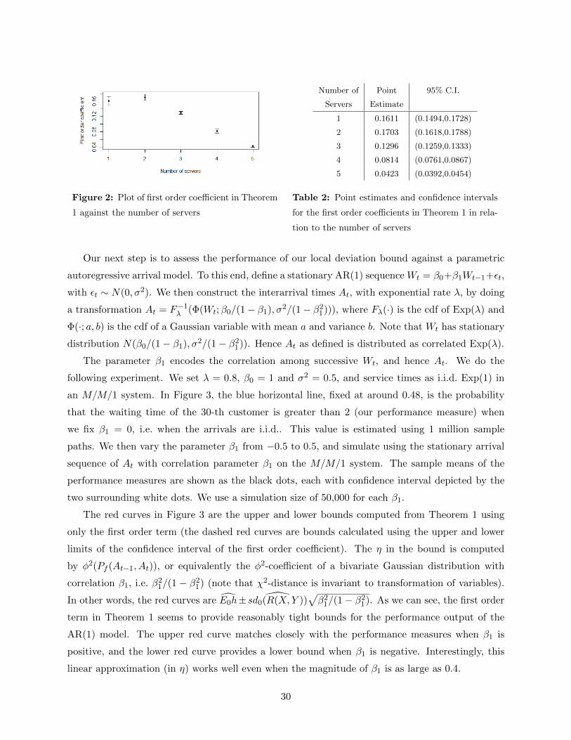
Figure 2: Plot of first order coefficient in Theorem

1 against the number of servers

Number of Point 95% C.I.

Servers Estimate

1 0.1611 (0.1494,0.1728)

2 0.1703 (0.1618,0.1788)

3 0.1296 (0.1259,0.1333)

4 0.0814 (0.0761,0.0867)

5 0.0423 (0.0392,0.0454)

Table 2: Point estimates and confidence intervals

for the first order coefficients in Theorem 1 in rela-

tion to the number of servers

Our next step is to assess the performance of our local deviation bound against a parametric

autoregressive arrival model. To this end, define a stationary AR(1) sequence Wt = β0+β1Wt−1+εt,

with εt ∼ N(0, σ2). We then construct the interarrival times At, with exponential rate λ, by doing

a transformation At = F−1λ (Φ(Wt;β0/(1− β1), σ2/(1− β2

1))), where Fλ(·) is the cdf of Exp(λ) and

Φ(·; a, b) is the cdf of a Gaussian variable with mean a and variance b. Note that Wt has stationary

distribution N(β0/(1− β1), σ2/(1− β21)). Hence At as defined is distributed as correlated Exp(λ).

The parameter β1 encodes the correlation among successive Wt, and hence At. We do the

following experiment. We set λ = 0.8, β0 = 1 and σ2 = 0.5, and service times as i.i.d. Exp(1) in

an M/M/1 system. In Figure 3, the blue horizontal line, fixed at around 0.48, is the probability

that the waiting time of the 30-th customer is greater than 2 (our performance measure) when

we fix β1 = 0, i.e. when the arrivals are i.i.d.. This value is estimated using 1 million sample

paths. We then vary the parameter β1 from −0.5 to 0.5, and simulate using the stationary arrival

sequence of At with correlation parameter β1 on the M/M/1 system. The sample means of the

performance measures are shown as the black dots, each with confidence interval depicted by the

two surrounding white dots. We use a simulation size of 50,000 for each β1.

The red curves in Figure 3 are the upper and lower bounds computed from Theorem 1 using

only the first order term (the dashed red curves are bounds calculated using the upper and lower

limits of the confidence interval of the first order coefficient). The η in the bound is computed

by φ2(Pf (At−1, At)), or equivalently the φ2-coefficient of a bivariate Gaussian distribution with

correlation β1, i.e. β21/(1 − β2

1) (note that χ2-distance is invariant to transformation of variables).

In other words, the red curves are E0h± sd0(R(X,Y ))√β2

1/(1− β21). As we can see, the first order

term in Theorem 1 seems to provide reasonably tight bounds for the performance output of the

AR(1) model. The upper red curve matches closely with the performance measures when β1 is

positive, and the lower red curve provides a lower bound when β1 is negative. Interestingly, this

linear approximation (in η) works well even when the magnitude of β1 is as large as 0.4.

30

Figure 3: Performance of the bounds in Theorem 1 against actual waiting time tail probabilities; red curves

are the bounds computed using the first order terms in (16) and (17)

We comment that the estimation of the coefficients in Theorem 1 using the nested simulation

approach, with the use of formula (50), is computationally intensive: to obtain one inner sample it

requires O(T 2) computational load. We believe that for large T , randomization of the time horizon

using formula (51) will better balance the computational burden with sampling accuracy. The

choice of sampling schemes, as well as the design of potential variance reduction techniques, will

be left to future investigation.

Lastly, we also ran experiment to estimate the second order coefficient in Theorem 1 for the

single-server setting with T = 10. We carried out the method described in Section 6.1, using

10, 000 samples of (s, t) pairs and for each (s, t) pair, we generated n = 2, 500 samples of Aj and Bj

respectively. The magnitude of the second order coefficient appears to be tiny. The sample mean of

(1/n)∑n

j=1Aj ·∑n

j=1Bj ·C using the 10, 000 trials is −1.1644×10−4, with a 95% confidence interval

(−6.8187× 10−4, 4.4900× 10−4) (which translates to −0.4636 for the second order coefficient after

multiplying by(T2

)and dividing by the estimate of V ar0(R(X,Y ))). We performed this estimation

several times (the above numeric comes from a typical output), and each time the 95% confidence

interval covers zero, which means statistically speaking the coefficient is no different from zero to

the degree of accuracy that the experiment can capture. In other words, the present method can

only suggest a very tiny second order effect. The exact magnitude of the second order coefficient

is yet to be determined, but it should be at most in the order of a tenth decimal place.

31

6.3 Numerical Example 2: Delta Hedging

Our next example is the delta hedging error for a European option. This setting was studied in

[11], who also considered a wide range of other problems in finance. Here our comparison focuses

on the case when the stock price of an underlying asset deviates from geometric Brownian motion

assumption to autoregressive type process, a structure that is amenable to the method studied in

this paper.

We adopt some notation from [11]. Consider a European call option, i.e. the payoff of the

option is (XT −K)+, where T is the maturity, Xtt≥0 is the stock price, and K is the strike price.

We assume a Black-Scholes benchmark model for the stock, namely that the stock price follows a

geometric Brownian motion

dXt = µXtdt+ σXtdBt

where Bt is a standard Brownian motion, µ is the growth rate of the stock, and σ is the volatility.

Assuming trading can be executed continuously over time without transaction fee, then it is well

known that a seller of the option at time 0 can perfectly hedge the payoff of the option by investing

δ(t,Xt) = Φ((log(Xt/K) + (r− (1/2)σ2)(T − t))/(σ√T − t)), i.e. the “delta”, units of stock at any

point of time, with the rest of the portfolio held as cash. Here r is the risk-free rate. This self-

balancing portfolio will exactly offset the payoff of the option at maturity. In practice, however,

trading cannot be done continuously, and implementing the Black-Scholes strategy will incur a

discretization error. To be more specific, suppose that trading is allowed at times k∆t for k =

0, 1, 2, . . . , T/(∆t), and that the trader holds the amount of cash C(0) and stock S(0):

C(0) = BS(0, T,X0)−X0δ(0, X0)

S(0) = X0δ(0, X0)

at time 0, and cash C(k∆t) and stock S(k∆t):

C(k∆t) = er∆tC((k − 1)∆t)−Xk∆t[δ(k∆, Xk∆t)− δ((k − 1)∆t,X(k−1)∆t)]

S(k∆t) = Xk∆tδ(k∆t,Xk∆t)

at time k∆t. Here BS(0, T,X0) is the Black-Scholes price for a European call option with maturity

T and initial stock price X0, and δ(k∆t,Xk∆t) is the “delta” of the option at time k∆t with current

stock price Xk∆t. The delta hedging error is given by

He = (XT −K)+ − C(T )− S(T )

and the performance measure is set to be E|He|.We consider the case when Xk∆t deviates from i.i.d. lognormal distribution to 1-dependent

process. Although |He| is unbounded in theory, and hence violating the assumption in Theorem 1,

32

for all practical purpose (and in all the simulation runs we have done) this variable only takes small

numbers. Hence the boundedness technicality should not be a concern in applying our proposed

method (for anxious users, one can merely consider a truncated hedging error as the cost function

by putting a large enough cap on |He|, which would not alter any of our simulation results). Figure

4 depicts the performance of the first order term in Theorem 1 against an AR(1) model. We use

T = 1 and ∆t = 0.01, so that the number of periods in consideration is 100. The initial stock

price and the strike price are both set to be 100, i.e. the call option is at-the-money. We set the

benchmark geometric Brownian motion to have growth rate µ = 0.1 and volatility σ =√

0.2, and

the risk-free rate as r = 0.05. The first order term of the bound in Theorem 1 is computed by using

1, 000 outer samples, 200 inner samples and 20 macro replications, which gives a point estimate of

1.5477, with 95% confidence interval (1.3820, 1.7134). The delta hedge error at the benchmark is

estimated to be 0.5021 from 100, 000 sample paths, which is depicted by the blue horizontal line in

Figure 4. The brown curves in the figure are the upper and lower bounds calculated using only the

first order term in Theorem 1. As a comparison to our bound, we compute E|He| for Xk∆t’s that

has logarithmic increment satisfying an AR(1) model, i.e. ∆ logXt = β0 +β1∆ logXt−1 +εt with β1

ranging from −0.2 to 0.2, and the stationary distribution kept at lognormal((µ−(1/2)σ2)∆t, σ2∆t).

The black dots in Figure 4 show the point estimates of E|He| at different β1, with the two bars

above and below each point depicting the 95% confidence interval. Each point estimate is obtained

using 20, 000 sample paths. Similar to the example in the previous subsection, the η in our bound

is set to be φ2(Pf (∆ logXt−1,∆ logXt)) for each β1. One can see that as β1 moves from negative to

positive, the hedging error generally decreases. The brown curves provide valid covering interval for

the hedging error throughout the whole range of β1 from −0.2 to 0.2. The upper curve is especially

tight in the negative region, with the curve almost touching the trend of black dots all the way to

β1 = −0.2.

Next, we compare our bounds to the method suggested in [11], which considers general model

uncertainty quantification. This comparison aims to demonstrate the gain in accuracy when assess-

ment scheme is derived in a way that targets at specific statistical feature, namely serial dependency

in this paper. The method in [11] is based on relative entropy. Part of their work suggested viewing

the sample path Xk∆t as a single random object and solving the optimization problem (adapted

to our notation) maxEf [h(Xk∆t)], where the optimization is over a Kullback-Leibler constraint

D(Pf (Xk∆t)‖P0(Xk∆t)) ≤ η. The optimal solution to this program is characterized by an ex-

ponential change of measure ∝ exph(Xk∆t)/α, where α > 0 is the dual optimal solution. For

a deviation from i.i.d. lognormal to AR(1) model over T time steps (while keeping the stationary

distribution unchanged), the involved Kullback-Leibler (KL) divergence on the sample path Xk∆can be calculated to be (T − 1) log(1/(1 − β2

1)) (we note that KL divergence is more convenient

33

Figure 4: Performance of the bounds in Theorem 1 against actual hedging error; brown curves are the

bounds computed using the first order terms in (16) and (17)

than χ2-distance when computing the model deviation of the whole sample path, since the former

is decomposable as the sum of individual divergences).

The green dashed curves in Figure 5 depicts the bound obtained from solving the above opti-

mization problem. To compute this bound for each value of β1, or the corresponding η, we first

approximately solve for the inverse of the optimal dual solution, i.e. 1/α > 0, via a sample average

approximation using 100, 000 benchmark sample paths. This can be done either by setting the

complementarity condition or by minimizing the dual program, both of which lead to identical

result. Then we average the 100, 000 sample paths using the exponential tilting weights with the

tilting parameter being the estimated 1/α, which gives the upper green curve. The lower green

curve is obtained analogously by solving for a negative 1/α. We can see that the green curves

bound the black dots that represent the actual hedging errors as β1 varies.

The brown curves in Figure 5 are the first order bounds in Theorem 1, i.e. the same brown

curves as in Figure 4. The increase in the tightness of the bounds is quite substantial; for example,

the gap goes down from a single digit to the order of one tenth in the case β1 = ±0.2. This suggests

that the bound in Theorem 1 is much more accurate in assessing the effect of first order dependency

compared to a general aggregate KL constraint. Of course, this is because we have made a stronger

structural assumption on model discrepancy and have devised a specialized method, whereas the

general bound in [11] treats the whole trajectory as a single object, and as such they are robust

against deviations other than serial dependency. This phenomenon highlights the tradeoff between

robustness and accuracy: for a user who is well-informed with the marginal distribution and who

is concerned about serial dependency, it is better off to adopt the approach in this paper to get

tighter error bound; on the other hand, a user who has only minimal knowledge about the sample

34

Figure 5: Comparison of the bounds in Theorem 1 and the method based on aggregate constraint not

targeted at serial dependency; brown curves are computed from Theorem 1, green curves are based on

aggregate constraint

path, including marginal distribution, could turn to the bound in [11] that is coarser but is capable

to safeguard against a wider sort of model misspecification.

We now test the performance of our sensitivity estimates for higher order dependency discussed

in Section 5. In particular, we focus on the bounds in Theorem 3, and compare it against a

parametric AR(2) model. Consider a stock price with logarithmic increment ∆ logXt = β0 +

β1∆ logXt−1 +β2∆ logXt−2 + εt. We allow β1 and β2 to vary, with β0 and the variance of εt chosen

so that the stationary distribution is kept at lognormal((µ− (1/2)σ2)∆t, σ2∆t).

Figure 6 compares our bounds with the AR(2) model when β1 is fixed at 0.1, and β2 varies

from −0.2 to 0.2. The black dots and the bars above and below them depict the point estimates

and the 95% confidence intervals of the actual hedging errors using 20, 000 sample paths. There is

a downward trend in the hedging error as β2 increases. Note that when β2 = 0, it reduces to an

AR(1) model. The green dashed lines are the upper and lower bounds computed using only the

first order coefficient in Theorem 1, or in other words, the bounds that are suitable for only first

order dependency assessment. As we can see, they provide a valid covering interval for the case

β2 = 0: the lower green line almost touches the black dot. However, when β2 moves away from 0,

the interval between the lines no longer contain the black dots, suggesting that the model under

scrutiny goes beyond first order dependency.

Encouragingly, our bounds are effective once we extend them to second order dependency effect.

The two brown curves in Figure 6 are computed from the upper and lower bounds in Theorem 3. The

second order coefficient in (40) and (41) is estimated to be 0.8879, with a 95% confidence interval

of (0.8687, 0.9071), using 1, 000 outer samples, 200 inner samples and 20 macro replications. The

35

η1 in the formula is set to be β21/(1 − β2

1), while the η2 parameter, which controls the deviation

from first to second order dependency, is numerically calculated using (37) and the observation in

Example 1. After adding the term controlling the second order dependency, we see that the brown

curves succeed in bounding the black dots. In fact, they seem to be reasonably tight, which also

suggests the approximate tightness of the inequalities in Theorem 3.

Figure 6: Performance of second order bounds in Theorem 3 against an AR(2) model as β2 varies; green

dashed lines are first order bounds computed using Theorem 1, and brown curves are second order bounds

computed using Theorem 3

As a further test, we also vary the value of β1 from −0.2 to 0.2, this time with β2 fixed at

0.1. Figure 7 shows our result. Again, the black dots and the bars locate the point estimates and

the 95% confidence intervals for the actual hedging errors, which show a downward trend as β1

increases. The green dashed curves are the upper and lower bounds computed using Theorem 1

with only the first order term, i.e. they are bounds that are targeted only for first order dependency.

When β1 = 0, the bounds degenerate to a single point at the benchmark performance measure.

When β1 deviates from 0, the bounds naturally widen, but still are not enough to contain the

black dots, especially for small positive β1. The brown curves depict the bounds computed using

Theorem 3, which covers the case of second order dependency. We see that there is an improvement

for the region of small positive β1. In particular, the lower bound is approaching the locations of

the black dots in this region.

7 Concluding Remarks

In this paper we propose a nonparametric, adversarial approach in quantifying the sensitivity of

input serial dependency to a stochastic system. The approach outputs local estimates for the

36

Figure 7: Performance of bounds in Theorem 3 against an AR(2) model as β1 varies; green dashed lines are

first order bounds computed using Theorem 1, and brown curves are second order bounds computed using

Theorem 3

worst- and best-case changes in system output subject to input deviation in terms of statistical

distance. These estimates are tight in the case of 1-dependency, and are in the form of conservative

bounds when higher order dependency is present. As we have mentioned in the introduction, the

approach that we are proposing is a general methodology: by placing appropriate constraints on the

associated optimization programs, other statistical features from the input model can be assessed.

One example of these other types of constraint is moment condition, which is widely used in

distributional robust optimization. In many practical situations, moments of the input model are

stably estimable from past data. Encapsulating such information can reduce input uncertainty and

help yielding less conservative error estimates. Analyzing this type of constraints thus constitutes

one of our future research directions. Moreover, one other important future direction is to extend

our framework beyond finite horizon problems, studied in the current paper, to other types of

system estimation, such as random horizon problems, steady-state and quantile estimation. We

believe that appropriate adaptation of the analysis proposed in this paper can bring in new insight

as well as practical tools to assess input model uncertainty for these other problem variations.

Lastly, we point out a potential use of our methodology that we have kept silent so far: the

construction of iterative method for computing bounds for more “global” assessment of model un-

certainty. The technique that we developed in this paper is clearly a local analysis. The assumption

that the input model only deviates in a neighborhood from the reality means that our method,

at least in theory, does not provide any guarantee for models that are far apart. One can argue

that this is a limitation of “derivative” type sensitivity analysis in general, and that in this case

the benchmark model should not be used in the first place. Nevertheless, we believe our local

37

analysis can potentially help assess model uncertainty even when the truth is far off, by suggesting

a well-defined local ascendency move in optimization problems that possess more “global” type of

distributional constraints. Notice that our results, such as Theorem 1, define a precise “steepest

descent” direction in the space of probability measures. Naturally, this points to the construction

of iterative scheme that converges to local optimum for optimization programs with similar kind

of dependency constraints. The construction of this sort of iterative schemes over the probability

space appears to be new.

A Selected Proofs

Proof of Proposition 2. The first step is to relax the constraints E0[L|x] = E0[L|y] = 1 a.s., and

consider

E0[h(X,Y )L]− α(E0(L− 1)2 − η) +

∫(E0[L|x]− 1)dβ(x) +

∫(E0[L|y]− 1)dγ(y) (54)

where β and γ are signed measures with bounded variation, i.e.∫|dβ|(x),

∫|dγ|(y) < ∞. Then,

differentiating (54) as a heuristic Euler-Lagrange equation gives

h(x, y)− 2αL(x, y) + β(x) + γ(y) = 0

which leads to

L =1

2α(h(x, y) + β(x) + γ(y)). (55)

Since E0[L] = 1, we must have E0[L] = 12α(E0[h(X,Y )] + E0β(X) + E0γ(Y )) = 1 or that

E0β(X) + E0γ(Y ) = 2α− E0[h(X,Y )]. (56)

Moreover, E0[L(X,Y )|x] = 1 and E0[L(X,Y )|y] = 1 give

1

2α(E0[h(X,Y )|x] + β(x) + E0γ(Y )) =

1

2α(E0[h(X,Y )|y] + E0β(X) + γ(y)) = 1

so that

β(x) = 2α− E0[h(X,Y )|x]− E0γ(Y ) (57)

γ(y) = 2α− E0[h(X,Y )|y]− E0β(Y ). (58)

Therefore, substituting (56), (57) and (58) into (55), we get

L(x, y) =1

2α(h(x, y) + 2α− E0[h(X,Y )|x]− E0γ(Y ) + 2α− E0[h(X,Y )|y]− E0β(Y ))

=1

2α(h(x, y) + 2α− E0[h(X,Y )|x] + 2α− E0[h(X,Y )|y]− 2α+ E0[h(X,Y )])

= 1 +1

2α(h(x, y)− E0[h(X,Y )|x]− E0[h(X,Y )|y] + E0h(X,Y )) (59)

38

which coincides with (10). The expression (59) is our candidate optimal solution, and our next

task is to verify that it is indeed an optimal solution. This means we have to prove that

E0[hL]− αE0(L− 1)2 ≤ E0[hL∗]− αE0(L∗ − 1)2 (60)

for any L ∈ L, where L∗ denotes the candidate optimal solution (59). To this end, recall the

notation in Section 3 that h = h− r, and that h possesses the orthogonal decomposition h = h+ r

on M⊥ ⊕M = L2. Then

E0[hL∗]− αE0(L∗ − 1)2 = E0h+1

2αE0[hr]− 1

4αE0r

2

= E0h+1

2αV ar0(r)− 1

4αV ar0(r) since h ⊥ r and E0r = 0

= E0h+1

4αV ar0(r)

Going back to (60), consider any L ∈ L. For convenience, we write U = L− 1 so that E0[U |X] =

E0[U |Y ] = E0U = 0 a.s.. Then we need to prove, for any such U ,

E0[h(U + 1)]− αE0U2 ≤ E0h+

1

4αV ar0(r)

⇔ E0[hU ]− αE0U2 ≤ 1

4αV ar0(r)

⇔ E0r2 − 4αE0[hU ] + 4α2E0U

2 ≥ 0

⇔ E0r2 − 4αE0[rU ]− 4αE0[hU ] + 4α2E0U

2 ≥ 0

⇔ E0(r − 2αU)2 − 4αE0[hU ] ≥ 0. (61)

But E0[hU ] = 0 since U ∈M. So (61) clearly holds.

Proof of Proposition 1. Since the formulation in (8) is convex, strong duality holds, so the optimal

value of (9) equals (8). By complementary slackness, we have α∗(E0(L∗ − 1) − η) = 0. Let us

assume for now that α∗ > 0, which implies E0(L∗ − 1)2 = η. From (10), this in turn implies

14α∗2

E0r2 = η or

1

4α∗2V ar0(r) = η (62)

since E0r = 0. Now the optimal objective value is

E0[hL∗] = E0

[h(

1 +r

2α∗

)]= E0h+

Cov0(h, r)

2α∗= E0h+

V ar0(r)

2α∗(63)

since h = h+ r with h orthogonal to r. Combining with (62), we get E0[hL∗] = E0h+ sd0(r)√η.

Lastly, suppose instead that α∗ = 0. Then the dual objective becomes maxL∈LE0[hL]. Since h

is non-constant, there exists a measurable set A ∈ supp(P0) ⊂ X 2 such that h(x, y) > E0[h] for any

(x, y) ∈ A. Now consider a feasible solution L ∈ L that has support on A. The resulting E0[hL]

39

must be strictly larger than E0[h]. Since we know, from (63), that as η → 0, the minimum dual

objective value E0[hL∗] over α > 0 can be arbitrarily close to E0[hL], we conclude that α∗ = 0 is

not possible.

Proof of Theorem 1. We follow the proof idea described at the end of Section 4. We first use the

complementarity condition to find the relation between η and α, which allows us to use Theorem

2. This will then also facilitate our expansion of the objective value in terms of η. Now recall from

(25) that L∗ satisfies L∗(x, y) = 1 + RL∗ (x,y)2α . We start with

HL∗(x, y)

=T∑t=2

E0

h ∏s=2,...,Ts 6=t

(1 +

RL∗(Xs−1, Xs)

2α

) ∣∣∣∣∣Xt−1 = x,Xt = y

=

T∑t=2

E0[h|Xt−1 = x,Xt = y] +1

2α

∑s,t=1,...,T

s 6=t

E0[hRL∗(Xs−1, Xs)|Xt−1 = x,Xt = y] + O

(1

α2

)

where O(1/αq) for q > 0 satisfies |O(1/αq)αq| ≤ C for some C, for any α > 0,

uniformly over x and y; the equality follows from the boundedness of RL∗(x, y)

inherited from h

= H2(x, y) +1

2αWL∗(x, y) + O

(1

α2

)(64)

where H2(x, y) =∑T

t=1E0[h|Xt−1 = x,Xt = y] is defined in (12), and

WL∗(x, y) =∑

s,t=1,...,Ts 6=t

E0[hRL∗(Xs−1, Xs)|Xt−1 = x,Xt = y].

Now, through a “filtering” of the linear effect of X and Y , (64) implies

RL∗(x, y) = R(x, y) +

SL∗(x, y)

2α+ O

(1

α2

)(65)

where RL and R are defined in (26) and (15), and

SL∗(x, y) = WL∗(x, y)− E0[WL∗ |x]− E0[WL∗ |y] + E0W

L∗ .

Therefore we can write

E0(L∗ − 1)2 = E0

(RL∗(X,Y )

2α

)2

=1

4α2E0

(R(X,Y ) +

SL∗(X,Y )

2α+ O

(1

α2

))2

=1

4α2

(E0R(X,Y )2 +

1

αE0[R(X,Y )SL

∗(X,Y )] +O

(1

α2

)).

40

Hence setting E0(L∗ − 1)2 = η gives

1

2α=

√η

sd0(R(X,Y ))

(1 +

1

α

E0[R(X,Y )SL∗(X,Y )]

V ar0(R(X,Y ))+O

(1

α2

))−1/2

since E0R(X,Y ) = 0

=

√η

sd0(R(X,Y ))

(1− 1

2α

E0[R(X,Y )SL∗(X,Y )]

V ar0(R(X,Y ))+O

(1

α2

))=

√η

sd0(R(X,Y ))− E0[R(X,Y )SL

∗(X,Y )]η

V ar0(R(X,Y ))2+O(η3/2) (66)

by recursing the expression. Note that the asymptotic is valid since we assume sd0(R(X,Y )) > 0.

This also shows that given any small enough η > 0, we can find α and L that satisfies E0(L∗−1)2 =

η, which allows us to invoke Theorem 2.

Now consider the objective value of (18):

E0[hL∗] = E0

[h

T∏t=2

(1 +

RL∗(Xt−1, Xt)

2α

)]

= E0h+1

2α

T∑t=2

E0[hRL∗(Xt−1, Xt)] +

1

4α2

∑s,t=2,...,T

s<t

E0[hRL∗(Xt−1, Xt)R

L∗(Xs−1, Xs)]

+O

(1

α3

). (67)

Using (65), we can write (67) as

E0h+1

2α

T∑t=2

E0[hR(Xt−1, Xt)] +1

4α2

T∑t=2

E0[hSL∗(Xt−1, Xt)]

+1

4α2

∑s,t=2,...,T

s<t

E0[hRL∗(Xt−1, Xt)R

L∗(Xs−1, Xs)] +O

(1

α3

)

= E0h+1

2αE0[H2(X,Y )R(X,Y )] +

1

4α

(E0[H2(X,Y )SL

∗]

+∑

s,t=2,...,Ts<t

E0[hR(Xs−1, Xs)R(Xt−1, Xt)]

)+O

(1

α3

)(68)

by conditioning on (Xt−1, Xt) inside some of the expectations to get the equality. Note that

E0[H2(X,Y )R(X,Y )] = V ar0(R(X,Y )), by the property that R is an orthogonal projection of H.

41

Then, by substituting (66), we have (68) equal to

E0h+ sd0(R(X,Y ))√η − E0[R(X,Y )SL

∗(X,Y )]η

V ar0(R(X,Y ))+

η

V ar0(R(X,Y ))E0[H(X,Y )SL∗(X,Y )] +

∑s,t=2,...,T

s<t

E0[hR(Xs−1, Xs)R(Xt−1, Xt)]

+O(η3/2)

= E0h+ sd0(R(X,Y ))√η +

η

V ar0(R(X,Y ))

(E0[H2(X,Y )SL

∗(X,Y )]− E0[R(X,Y )SL

∗(X,Y )]

+∑

s,t=2,...,Ts<t

E0[hR(Xs−1, Xs)R(Xt−1, Xt)]

)+O(η3/2) (69)

Now note that H −R is orthogonal to SL∗

by construction. This concludes that (69) is equal to

E0h+ sd0(R(X,Y ))√η +

η

V ar0(R(X,Y ))

∑s,t=2,...,T

s<t

E0[hR(Xs−1, Xs)R(Xt−1, Xt)] +O(η3/2)

which gives the theorem.

References

[1] S. Asmussen and P. W. Glynn. Stochastic simulation: Algorithms and analysis, volume 57.

Springer, 2007.

[2] D. Bertsekas. Dynamic programming and optimal controlvolume 2, 4th edition, 2012.

[3] B. Biller and B. L. Nelson. Fitting time-series input processes for simulation. Operations

Research, 53(3):549–559, 2005.

[4] M. C. Cario and B. L. Nelson. Autoregressive to anything: Time-series input processes for

simulation. Operations Research Letters, 19(2):51–58, 1996.

[5] N. H. Chan and L. T. Tran. Nonparametric tests for serial dependence. Journal of Time Series

Analysis, 13(1):19–28, 1992.

[6] D. R. Cox and N. Reid. The theory of the design of experiments. CRC Press, 2002.

[7] E. Delage and Y. Ye. Distributionally robust optimization under moment uncertainty with

application to data-driven problems. Operations Research, 58(3):595–612, 2010.

[8] E. Erdogan and G. Iyengar. Ambiguous chance constrained problems and robust optimization.

Mathematical Programming, 107(1-2):37–61, 2006.

42

[9] P. Fillmore and J. Williams. On operator ranges. Advances in Mathematics, 7(3):254–281,

1971.

[10] S. Ghosh and S. G. Henderson. Chessboard distributions and random vectors with specified

marginals and covariance matrix. Operations Research, 50(5):820–834, 2002.

[11] P. Glasserman and X. Xu. Robust risk measurement and model risk. Available at SSRN

2167765, 2012.

[12] J. Goh and M. Sim. Distributionally robust optimization and its tractable approximations.

Operations Research, 58(4-Part-1):902–917, 2010.

[13] C. Granger and J.-L. Lin. Using the mutual information coefficient to identify lags in nonlinear

models. Journal of time series analysis, 15(4):371–384, 1994.

[14] C. Granger, E. Maasoumi, and J. Racine. A dependence metric for possibly nonlinear processes.

Journal of Time Series Analysis, 25(5):649–669, 2004.

[15] J. D. Hamilton. Time series analysis, volume 2. Cambridge Univ Press, 1994.

[16] F. R. Hampel. The influence curve and its role in robust estimation. Journal of the American

Statistical Association, 69(346):383–393, 1974.

[17] F. R. Hampel, E. M. Ronchetti, P. J. Rousseeuw, and W. A. Stahel. Robust statistics: the

approach based on influence functions, volume 114. Wiley. com, 2011.

[18] L. P. Hansen and T. J. Sargent. Robustness. Princeton university press, 2008.

[19] J. Hong and S. Juneja. Kernel smoothing for nested estimation with application to portfolio

risk measurement. Working paper.

[20] Y. Hong and H. White. Asymptotic distribution theory for nonparametric entropy measures

of serial dependence. Econometrica, 73(3):837–901, 2005.

[21] G. N. Iyengar. Robust dynamic programming. Mathematics of Operations Research, 30(2):257–

280, 2005.

[22] H. Lam. Robust sensitivity analysis for stochastic systems. arXiv preprint arXiv:1303.0326,

2013.

[23] H. Lam and S. Ghosh. Iterative method for robust estimation under bivariate distributional

uncertainty. In to appear in Proceedings of the 2013 Winter Simulation Conference (WSC).

43

[24] M. Livny, B. Melamed, and A. K. Tsiolis. The impact of autocorrelation on queuing systems.

Management Science, 39(3):322–339, 1993.

[25] D. G. Luenberger. Optimization by Vector Space Methods. Wiley, 1969.

[26] J.-F. Mai and M. Scherer. Simulating Copulas: Stochastic Models, Sampling Algorithms, and

Applications, volume 4. World Scientific, 2012.

[27] C. Mitchell, A. Paulson, and C. Beswick. The effect of correlated exponential service times on

single server tandem queues. Naval Research Logistics Quarterly, 24(1):95–112, 1977.

[28] A. Nemirovski and A. Shapiro. Convex approximations of chance constrained programs. SIAM

Journal on Optimization, 17(4):969–996, 2006.

[29] A. Nilim and L. El Ghaoui. Robust control of markov decision processes with uncertain

transition matrices. Operations Research, 53(5):780–798, 2005.

[30] I. R. Petersen, M. R. James, and P. Dupuis. Minimax optimal control of stochastic uncer-

tain systems with relative entropy constraints. Automatic Control, IEEE Transactions on,

45(3):398–412, 2000.

[31] J. Pinkse. A consistent nonparametric test for serial independence. Journal of Econometrics,

84(2):205–231, 1998.

[32] Y. Sun, D. W. Apley, and J. Staum. Efficient nested simulation for estimating the variance of

a conditional expectation. Operations research, 59(4):998–1007, 2011.

B Proofs of Technical Results

B.1 Equivalence of Formulations

Detailed justification of the equivalence between (5) and (8). We show that, for any feasible solu-

tion in the max program in (5), one can find a feasible solution in (8) that attains the same objective

value, and vice versa. First, given any Pf that has the same marginal distributions as P0, we can

let L(X,Y ) = dPf (X,Y )/dP0(X,Y ) = dPf (X,Y )/dPf (X)dPf (Y ). Then φ2(Pf ) ≤ η is equivalent

to E0(L − 1)2 ≤ η. Also, as discussed in Section 3, Pf (x) = P0(x) implies E0[L|X] = 1 a.s. since

Pf (X ∈ A) = E0[E0[L|X]I(X ∈ A)], and similarly Pf (y) = P0(y) implies E0[L|Y ] = 1 a.s..

On the other hand, given any L in the feasible set in (8), we define Pf (x, y) = L(x, y)dP0(x)dP0(y).

The constraint E0(L− 1)2 ≤ η implies immediately that φ2(Pf ) ≤ η. Moreover,

Pf (X ∈ A) = E0[L(X,Y )I(X ∈ A)] = E0[E0[L|X]I(X ∈ A)] = P0(X ∈ A)

44

since E0[L|X] = 1 a.s.. Similarly, Pf (Y ∈ B) = P0(Y ∈ B) for any measurable B.

Hence the two formulations are equivalent.

Proof of Proposition 3. We prove in both directions. First, we show that each feasible solution in

(11) can be re-expressed as a feasible solution in (18) that has the same objective value. Given Pf

that satisfies Pf (xt) = P0(xt), we can let Lt(xt−1, xt) = dPf (xt|xt−1)/dP0(xt) = dPf (xt−1, xt)/dP0(xt−1)Pf (xt)

be the likelihood ratio of a transition step under Pf w.r.t. the benchmark. Since Pf (xt) = P0(xt), we

have Lt(xt−1, xt) = dPf (xt−1, xt)/dP0(xt−1)P0(xt) = dPf (xt−1, xt)/dPf (xt−1)Pf (xt). Also, since

Pf (xt−1, xt) = Pf (xs−1, xs) for all s, t, this means that Lt(·, ·) are all the same, so we can let L be

the identical likelihood ratio. Then

Ef [h(XT )] =

∫h(xT )dPf (x1)dPf (x2|x1) · · · dPf (xT |xT−1)

=

∫h(xT )

dPf (x1)

dP0(x1)

dPf (x2|x1)

dP0(x2)· · ·

dPf (xT |xT−1)

dP0(xT )dP0(x1) · · · dP0(xT )

=

∫h(xT )L(x1, x2) · · ·L(xT−1, xT )dP0(x1) · · · dP0(xT )

= E0

[h(XT )

T∏t=2

L(Xt−1, Xt)

].

Hence the objectives are the same. To show that L is feasible, first note that φ2(Pf (X,Y )) =

E(L(X,Y ) − 1)2 by the definition of L, so φ2(Pf (X,Y )) ≤ η implies E(L(X,Y ) − 1)2 ≤ η. Now,

much like the justification of (8), since

Pf (Xt−1 ∈ A) = E0[E0[L(Xt−1, Xt)|Xt−1]I(Xt−1 ∈ A)] = P0(Xt ∈ A)

for any measurableA, by the constraint that Pf (Xt−1) = P0(Xt−1), we must have E0[L(Xt−1, Xt)|Xt−1] =

1. Similarly, E0[L(Xt−1, Xt)|Xt] = 1. Hence L satisfies all the constraints in (18).

To prove the other direction, given any L in the feasible set of (18), define the Markov transition

kernel dPf (xt|xt−1) = L(xt−1, xt)dP0(xt) for any t = 2, . . . , T , and dPf (x1) = dP0(x1). Note that

dPf (xt|xt−1) is well-defined since∫dPf (xt|xt−1) =

∫L(xt−1, xt)dP0(xt) = E0[L(xt−1, xt)|xt−1] = 1

a.e., by the first marginal constraint in (18). Now

E0

[h(XT )

T∏t=2

L(Xt−1, Xt)

]=

∫h(xT )dP0(x1)

T∏t=2

L(xt−1, xt)dP0(xt)

=

∫h(xT )dPf (x1)

T∏t=2

dPf (xt|xt−1)

= Ef [h(XT )].

45

Hence the objective is matched. Next we prove Pf (xt) = P0(xt) by induction. Note that Pf (X1 ∈A) = P0(X1 ∈ A) for any measurable A by definition. Assume Pf (xt−1) = P0(xt−1). Then

Pf (Xt ∈ A) =

∫xt∈A

dPf (xt|xt−1)dPf (xt−1)

=

∫xt∈A

L(xt−1, xt)dP0(xt)dP0(xt−1)

=

∫xt∈A

E0[L(Xt−1, Xt)|Xt = xt]dP0(xt)

= P0(Xt ∈ A)

for any measurable A, by the second marginal constraint in (18). Hence Pf (xt) = P0(xt), and we

conclude our induction.

Finally, note that dPf (Xt|Xt−1) = L(Xt−1, Xt)dP0(Xt) implies L = dPf (Xt|Xt−1)/dP0(Xt) =

dPf (Xt−1, Xt)/dP0(Xt−1)P0(Xt). Hence E0(L(X,Y )− 1)2 ≤ η implies φ2(Pf (X,Y )) ≤ η.

B.2 Proofs Related to the Contraction and Fixed Point Machinery

We first point out some convenient properties of L, which defines a change of measure sequentially

from the i.i.d. samples in P0 to the Markov chain under Pf , over the time steps t = 1, 2, . . . , T . Note

that this definition is two-way, i.e. a Markov chain can be constructed both forward and backward

in time under stationarity. Moreover, the chain can be started from any time point conditioned

on stationarity. Let us now define Ls:t =∏tk=s L(Xk−1, Xk) for any 2 ≤ s ≤ t ≤ T . Also, for

any 1 ≤ s ≤ t ≤ T , define Fs:t = F(Xs, . . . , Xt) as the σ-algebra generated by Xs, . . . , Xt. The

following two properties of Ls:t are immediate:

Lemma 4. 1. Under P0, and fix the starting point of time 2 ≤ s ≤ T under stationarity. The

process Ls:t : t = s−1, s, s+1, . . . (where we define Ls:(s−1) = 1) is a martingale adapted to

F(s−1):t : t = s− 1, s, s+ 1, . . ., with initial value identical to 1. Similar property holds for

the time-reverse setting. Namely, under P0, and fix the starting time 2 ≤ t ≤ T . The process

Ls:t : s = t + 1, t, t − 1, . . . (where we now define L(t+1):t = 1) is a martingale adapted to

F(s−1):t : s = t+ 1, t, t− 1, . . . with initial value 1.

2. For any measurable g(Xs:t) := g(Xs, . . . , Xt), for s ≤ t, we have

Ef [g(Xs:t)] = E0[g(Xs:t)L2:t] = E0[g(Xs:t)L(s+1):T ].

Both properties can be generalized to the scenario when the factors L in the likelihood ratio

product Ls:t are non-identical.

46

Proof of Lemma 4. To prove the first part, consider, for any t ≥ s,

E0[Ls:(t+1)|F(s−1):t] = E0[L(Xs−1, Xs) · · ·L(Xt, Xt+1)|F(s−1):t]

= L(Xs−1, Xs) · · ·L(Xt−1, Xt)E0[L(Xt, Xt+1)|F(s−1):t]

= L(Xs−1, Xs) · · ·L(Xt−1, Xt)

since E0[L(Xt, Xt+1)|F(s−1):t] = E0[L(Xt, Xt+1)|Xt] = 1

by the first marginal constraint in (18)

= Ls:t

The backward direction follows analogously, by using the second marginal constraint in (18). The

second part of the lemma follows immediately from the forward and backward martingale properties

of Ls:t. Also, the generalization to non-identical L’s follows trivially.

Proof of Lemma 1. We divide the proofs into three components: first, we show that K is well-

defined and closed; second, we prove that K is a contraction map; lastly, we show that the fixed

point of K has all identical components.

We start with showing well-definedness. Note that each summand in the definition ofHL(1):(T−2)(x, y)

satisfies

|E0[hL(T−t+1)(X1, X2)L(T−t+2)(X2, X3) · · ·L(T )(Xt−2, Xt−1)L(1)(Xt, Xt+1)L(2)(Xt+1, Xt+2)

· · ·L(T−t)(XT−1, XT )|Xt−1 = x,Xt = y]|

≤ CE0[L(T−t+1)(X1, X2)L(T−t+2)(X2, X3) · · ·L(T )(Xt−2, Xt−1)L(1)(Xt, Xt+1)L(2)(Xt+1, Xt+2)

· · ·L(T−t)(XT−1, XT )|Xt−1 = x,Xt = y] for some C > 0

= CE0[L(T−t+1)(X1, X2)L(T−t+2)(X2, X3) · · ·L(T )(Xt−2, Xt−1)|Xt−1 = x]

E0[L(1)(Xt, Xt+1)L(2)(Xt+1, Xt+2) · · ·L(T−t)(XT−1, XT )|Xt = y]

= C by the forward and backward martingale properties of Lemma 4.

Hence |HL(1):(T−2)(x, y)| ≤ (T − 1)C, and the stepwise operator K satisfies

|K(L(1):(T−2))− 1| ≤ 4(T − 1)C

2α<∞.

The same bound holds for each K(L(1), L(2), . . . , L(t), L(t+1), . . . , L(T−2)) for t = 1, . . . , T−3. Hence

each component of K(L(1):(T−2)) is finite a.s.. Moreover, for large enough α, we have

|HL(1):(T−2)

(x, y)− E0[HL(1):(T−2)

|x]− E0[HL(1):(T−2)

|y] + E0HL(1):(T−2)

| ≤ 4(T − 1)C ≤ 2α

for any L(1):(T−2) ∈ Lc(M)T−2 and so each component of K(L(1):(T−2)) is non-negative a.s.. Note

that by definition K(L(1):(T−2)) satisfies E0[K(L(1):(T−2))|x] = E0[K(L(1):(T−2))|y] = 1 a.s., and

similarly along the iteration of K in (29).

47

To conclude that K is well-defined, we are left to show that K preserves the boundedness in the

L2-norm. Since

E0K(L(1):(T−2))2 − 1 = E0(K(L(1):(T−2))− 1)2

=1

4α2E0

(HL(1):(T−2)

(X,Y )− E0[HL(1):(T−2)

|X]− E0[HL(1):(T−2)

|Y ] + E0HL(1):(T−2)

)2

≤ (4(T − 1)C)2

4α2

≤ M − 1

for any L(1):(T−2) ∈ Lc(M)T−2, when α is large enough, we have K(L(1):(T−2)) ∈ Lc(M). Iterating

through K(L(1), L(2), . . . , L(t), L(t+1), . . . , L(T−2)) for t = 1, . . . , T − 3, we conclude that K is closed

in Lc(M)T−2.

Now we show that K is a contraction. Consider, for any L(1):(T−2) = (L(1), . . . , L(T−2)) ∈Lc(M)T−2 and L(1):(T−2)′ = (L(1)′ , . . . , L(T−2)′) ∈ Lc(M)T−2,

E0|K(L(1):(T−2))−K(L(1):(T−2)′)|2

≤ E0|HL(1):(T−2)

−HL(1):(T−2)′|2 since projection is a contraction

≤ C

4α2E0

( T∑t=2

E0[|Lt − L′t||Xt−1, Xt]

)2

≤ (T − 1)2C

4α2

T∑t=2

E0

(E0[|Lt − L′t||Xt−1, Xt]

)2(70)

for some constant C > 0, where we denote

Lt = L(T−t+1)(X1, X2)L(T−t+2)(X2, X3) · · ·L(T )(Xt−2, Xt−1)L(1)(Xt, Xt+1)L(2)(Xt+1, Xt+2)

· · ·L(T−t)(XT−1, XT )

and

L′t

= L(T−t+1)′(X1, X2)L(T−t+2)′(X2, X3) · · ·L(T )′(Xt−2, Xt−1)L(1)′(Xt, Xt+1)L(2)′(Xt+1, Xt+2)

· · ·L(T−t)′(XT−1, XT )

for convenience.

48

Let us focus on E0

(E0[|Lt − L′t||Xt−1, Xt]

)2. Note that, by telescoping, we have

Lt − L′t

=(L(T−t+1)(X1, X2)− L(T−t+1)′(X1, X2)

)L(T−t+2)(X2, X3) · · ·L(T )(Xt−2, Xt−1)L(1)(Xt, Xt+1)

L(2)(Xt+1, Xt+2) · · ·L(T−t)(XT−1, XT )

+ L(T−t+1)′(X1, X2)

(L(T−t+2)(X2, X3) · · ·L(T )(Xt−2, Xt−1)L(1)(Xt, Xt+1)L(2)(Xt+1, Xt+2)

· · ·L(T−t)(XT−1, XT )

− L(T−t+2)′(X2, X3) · · ·L(T )′(Xt−2, Xt−1)L(1)′(Xt, Xt+1)L(2)′(Xt+1, Xt+2) · · ·L(T−t)′(XT−1, XT )

)...

=∑

s=2,...,Ts 6=t

s−1∏k=2k 6=t

L(k−t)′(Xk−1, Xk)(L(s−t)(Xs−1, Xs)− L(s−t)′(Xs−1, Xs)

) T∏k=s+1k 6=t

L(k−t)(Xk−1, Xk)

where we denote L(k) for a negative k to be L(k+T−1). Hence

E0[|Lt − L′t||Xt−1, Xt]

≤∑

s=2,...,Ts 6=t

E0

[s−1∏k=2k 6=t

L(k−t)′(Xk−1, Xk)∣∣∣L(s−t)(Xs−1, Xs)− L(s−t)′(Xs−1, Xs)

∣∣∣ T∏k=s+1k 6=t

L(k−t)(Xk−1, Xk)

∣∣∣∣∣Xt−1, Xt

]

and so

E0

(E0[|Lt − L′t||Xt−1, Xt]

)2

≤ (T − 2)2∑

s=2,...,Ts 6=t

E0

(E0

[s−1∏k=2k 6=t

L(k−t)′(Xk−1, Xk)∣∣∣L(s−t)(Xs−1, Xs)− L(s−t)′(Xs−1, Xs)

∣∣∣T∏

k=s+1k 6=t

L(k−t)(Xk−1, Xk)

∣∣∣∣∣Xt−1, Xt

])2

. (71)

Let us now consider each summand above. Without loss of generality, consider the case s < t. We

49

have

E0

s−1∏k=2

L(k−t)′(Xk−1, Xk)∣∣∣L(s−t)(Xs−1, Xs)− L(s−t)′(Xs−1, Xs)

∣∣∣ T∏k=s+1k 6=t

L(k−t)(Xk−1, Xk)

∣∣∣∣∣Xt−1, Xt

= E0

[s−1∏k=2

L(k−t)′(Xk−1, Xk)∣∣∣L(s−t)(Xs−1, Xs)− L(s−t)′(Xs−1, Xs)

∣∣∣ t−1∏k=s+1

L(k−t)(Xk−1, Xk)

∣∣∣∣∣Xt−1

]

E0

[T∏k=t

L(k−t)(Xk−1, Xk)

∣∣∣∣∣Xt

]

where we denotet−1∏

k=s+1

L(k−t)(Xk−1, Xk) = 1 if s = t− 1

= E0

[s−1∏k=2

L(k−t)′(Xk−1, Xk)∣∣∣L(s−t)(Xs−1, Xs)− L(s−t)′(Xs−1, Xs)

∣∣∣ t−1∏k=s+1

L(k−t)(Xk−1, Xk)

∣∣∣∣∣Xt−1

]

sinceT∏k=t

L(k−t)(Xk−1, Xk) is a forward martingale by Lemma 4;

= E0

[E0

[s−1∏k=2

L(k−t)′(Xk−1, Xk)∣∣∣L(s−t)(Xs−1, Xs)− L(s−t)′(Xs−1, Xs)

∣∣∣ t−1∏k=s+1

L(k−t)(Xk−1, Xk)∣∣∣∣∣Fs:(t−1)

]∣∣∣∣∣Xt−1

]

= E0

[E0

[s−1∏k=2

L(k−t)′(Xk−1, Xk)∣∣∣L(s−t)(Xs−1, Xs)− L(s−t)′(Xs−1, Xs)

∣∣∣ ∣∣∣∣∣Xs

]t−1∏

k=s+1

L(k−t)(Xk−1, Xk)

∣∣∣∣∣Xt−1

]

= Ef

[E0

[s−1∏k=2

L(k−t)′(Xk−1, Xk)∣∣∣L(s−t)(Xs−1, Xs)− L(s−t)′(Xs−1, Xs)

∣∣∣ ∣∣∣∣∣Xs

] ∣∣∣∣∣Xt−1

](72)

where Ef is under the change of measure generated by∏t−1k=s+1 L

(k−t)(Xk−1, Xk). On the other

hand, we have

E0

[s−1∏k=2

L(k−t)′(Xk−1, Xk)∣∣∣L(s−t)(Xs−1, Xs)− L(s−t)′(Xs−1, Xs)

∣∣∣ ∣∣∣∣∣Xs

]

= E0

[E0

[s−1∏k=2

L(k−t)′(Xk−1, Xk)∣∣∣L(s−t)(Xs−1, Xs)− L(s−t)′(Xs−1, Xs)

∣∣∣ ∣∣∣∣∣Xs−1, Xs

] ∣∣∣∣∣Xs

]

= E0

[E0

[s−1∏k=2

L(k−t)′(Xk−1, Xk)

∣∣∣∣∣Xs−1

] ∣∣∣L(s−t)(Xs−1, Xs)− L(s−t)′(Xs−1, Xs)∣∣∣ ∣∣∣∣∣Xs

]

= E0

[∣∣∣L(s−t)(Xs−1, Xs)− L(s−t)′(Xs−1, Xs)∣∣∣ ∣∣∣∣∣Xs

](73)

50

by the backward martingale property of∏s−1k=2 L

(k−t)′(Xk−1, Xk). So, by (72), (73) and Jensen’s

inequality, we have

E0

(E0

[s−1∏k=2

L(k−t)′(Xk−1, Xk)∣∣∣L(s−t)(Xs−1, Xs)− L(s−t)′(Xs−1, Xs)

∣∣∣T∏

k=s+1

L(k−t)(Xk−1, Xk)

∣∣∣∣∣Xt−1, Xt

])2

= E0

(Ef

[E0

[∣∣∣L(s−t)(Xs−1, Xs)− L(s−t)′(Xs−1, Xs)∣∣∣ ∣∣∣∣∣Xs

] ∣∣∣∣∣Xt−1

])2

= E0

(E ˜f

[∣∣∣L(s−t)(Xs−1, Xs)− L(s−t)′(Xs−1, Xs)∣∣∣ ∣∣∣∣∣Xt−1

])2

≤ E0

[|L(s−t)(Xs−1, Xs)− L(s−t)′(Xs−1, Xs)|2

](74)

where E ˜f

denotes the expectation under the change of measure induced by∏t−1k=s+1 L

(k−t)(Xk−1, Xk)

from step t − 1 backward to s and then following the benchmark P0 before s. The last inequality

follows from Jensen’s inequality, and by the construction that Xs is marginally distributed as P0

and that the transition from Xs and Xs−1 is under the benchmark P0.

Therefore, (71) is bounded by

(T − 2)2∑

s=2,...,Ts 6=t

E0

[∣∣∣L(s−t)(Xs−1, Xs)− L(s−t)′(Xs−1, Xs)∣∣∣2] ,

and hence (70) is bounded by

(T − 1)2(T − 2)2C

4α2

T∑t=2

∑s=2,...,Ts 6=t

E0[|L(s−t)(Xs−1, Xs)− L(s−t)′(Xs−1, Xs)|2]

=(T − 1)3(T − 2)2C

4α2

T−2∑t=1

E0[|L(t) − L(t)′ |2]

≤ (T − 1)3(T − 2)3C

4α2d(L(1):(T−2), L(1):(T−2)′)2.

When α is large enough, this gives E0|K(L(1):(T−2))−K(L(1):(T−2)′)|2 ≤ d(L(1):(T−2), L(1):(T−2)′)2,

and the computation above can be iterated over (L(1), L(2), . . . , L(t), L(t+1), . . . , L(T−2)) for t =

1, . . . , T − 3. Then we shall get that

d(K(L(1):(T−2)),K(L(1):(T−2)′))2 ≤ (T − 1)3(T − 2)3C

4α2d(L(1):(T−2), L(1):(T−2)′)2

51

which gives

d(K(L(1):(T−2)),K(L(1):(T−2)′)) ≤ (T − 1)3/2(T − 2)3/2C1/2

2αd(L(1):(T−2), L(1):(T−2)′)

≤ cd(L(1):(T−2), L(1):(T−2)′)

for some constant 0 < c < 1, when α is large enough. Hence we conclude that K is a contraction

on Lc(M)T−2.

By Banach fixed point theorem, K has a fixed point L∗. We are left to show that all components

of L∗ are identical. To this end, let L∗ = (L(1)∗, L(2)∗, . . . , L(T−2)∗) and note that by the definition

of fixed point and the iteration in (29),

L(1)∗ := K(L(1)∗, L(2)∗, . . . , L(T−2)∗) = L(1)∗

L(2)∗ := K(L(1)∗, L(2)∗, . . . , L(T−2)) = K(L(1)∗, L(2)∗, . . . , L(T−2)∗) = L(2)∗

L(3)∗ := K(L(1)∗, L(2)∗, L(3)∗ . . . , L(T−2)) = K(L(1)∗, L(2)∗, L(3)∗ . . . , L(T−2)∗) = L(3)∗

...

L(T−2)∗ := K(L(1)∗, L(2)∗, . . . L(T−3)∗, L(T−2)) = K(L(1)∗, L(2)∗, . . . L(T−3)∗, L(T−2)∗) = L(T−2)∗

and hence

L(1)∗ = L(2)∗ = · · · = L(T−2)∗ = K(L(1)∗, L(2)∗, . . . , L(T−2)∗).

We thus have concluded the lemma.

Proof of Lemma 3. We first note that, as discussed in Section 4.2, convergence to the fixed point

associated with the operator K under the d-metric implies componentwise convergence, i.e. the

sequence L(k) = K(L(k−T+2), L(k−T+3), . . . , L(k−1)) for k = T − 1, T − 2, . . . defined in Lemma 2

converges to L∗, the identical component of the fixed point L∗ of K.

Now consider each term in (32). For the first term,

HL(k):(k+T−2)

− HL∗ ≤ CT∑t=2

E0|Lk,t − L∗| (75)

for some constant C > 0, where we denote

Lk,t = L(k+T−t+2)(X1, X2)L(k+T−t+3)(X2, X3) · · ·L(k+T−1)(Xt−2, Xt−1)L(k+1)(Xt−1, Xt)

L(k+2)(Xt, Xt+1) · · ·L(k+T−t+1)(XT−1, XT )

and

L∗ =T∏t=2

L∗(Xt−1, Xt).

52

Then, by the same technique in the proof of contraction in Lemma 1, we have (75) bounded by

C

T∑t=2

T∑s=2

E0|L(k+s−t+1)(Xs−1, Xs)− L∗(Xs−1, Xs)|

where we denote L(k+j) = L(k+j+T−1) for any negative j, which is then equal to

C(T − 1)

T∑t=2

E0|L(k+t−2) − L∗| → 0

as k → ∞. For the second term in (32), since ‖L(k) − L∗‖2 → 0, we have immediately that

‖L(k)‖2 → ‖L∗‖2 and so

T∑t=2

E0(L(k+t−2) − 1)2 − (T − 1)E0(L∗ − 1)2 → 0

as k →∞. Hence we have proved the lemma.

B.3 Proofs Related to Higher Order Dependency Assessment

Missing component of proof for Theorem 3. As discussed in Section 5, in order to show Theo-

rem 3, we have to argue that S(X,Y, Z) is the projection of H0,2(X,Y, Z) onto M0 and that

sdf∗1(Sf∗1

(X,Y, Z)) → sd0(S(X,Y, Z)), where X, Y and Z are three consecutive states under the

respective measure. We lay out our argument for each of these below.

S(X,Y, Z) is a projection. We first check that S(X,Y, Z) ∈ M0. Note that from (42) we can write

S(x, y, z) = H0,2(x, y, z)− E0[H0,2|x, y]− E0[H0,2|y, z] + E0[H0,2|y].

So

E0[S(X,Y, Z)|X,Y ] = E0[H0,2|X,Y ]− E0[H0,2|X,Y ]− E0[H0,2|Y ] + E0[H0,2|Y ] = 0

since X and Z are independent. Similarly, E0[S(X,Y, Z)|Y, Z] = 0, and so S(X,Y, Z) ∈ M0.

53

Next we show that S and H0,2 − S are orthogonal. Consider

E0[S(H0,2 − S)]

= E0(H0,2(X,Y, Z)− E0[H0,2|X,Y ]− E0[H0,2|Y, Z] + E0[H0,2|Y ])

(E0[H0,2|X,Y ] + E0[H0,2|Y, Z]− E0[H0,2|Y ])

= E0(E0[H0,2|X,Y ])2 + E0(E0[H0,2|Y, Z])2 − E0(E0[H0,2|Y ])2

− E0(E0[H0,2|X,Y ] + E0[H0,2|Y,Z]− E0[H0,2|Y ])2

= −2E0[E0[H0,2|X,Y ]E0[H0,2|Y,Z]] + 2E0[E0[H0,2|X,Y ]E0[H0,2|Y ]]

+ 2E0[E0[H0,2|Y,Z]E0[H0,2|Y ]]− 2E0(E0[H0,2|Y ])2

= −2E0(E0[H0,2|Y ])2 + 2E0(E0[H0,2|Y ])2 + 2E0(E0[H0,2|Y ])2 − 2E0(E0[H0,2|Y ])2

= 0

where the second-to-last step is via conditioning on Y , and by using the fact that given Y ,

E0[H0,2|X,Y ] is independent of E0[H0,2|Y,Z]. Therefore S(X,Y, Z) is the projection of H0,2 onto

M0.

The convergence sdf∗1(Sf∗1

(X,Y, Z))→ sd0(S(X,Y, Z)). To facilitate the proof, denote P f∗1 as the

projection operator onto Mf∗1in the space L2(Pf∗1

), and similarly denote P0 as the projection onto

M0 in the space L2(P0). Note that since Ef∗1Sf∗1

= 0, sdf∗1(Sf∗1

) is exactly ‖Sf∗1 ‖f∗1 , where we

denote ‖ · ‖f∗1 as the L2(Pf∗1)-norm. In a similar fashion, sd0(S) = ‖S‖0, where we denote ‖ · ‖0

as the L2(P0)-norm. With these notations, we are set to prove that ‖P f∗1 Hf∗1 ,2‖f∗1 → ‖P

0H0,2‖0 as

η1 → 0.

Next, we observe that by the boundedness of h and that convergence in χ2-distance implies

convergence in distribution, we have Hf∗1 ,2(x, y, z)→ H0,2(x, y, z) pointwise a.e. as η1 → 0. Hence

by dominated convergence ‖Hf∗1 ,2− H0,2‖0 → 0, where Hf∗1 ,2

and H0,2 are coupled in the natural

way under the measure P0. Moreover, we have ‖G‖f∗1 → ‖G‖0 for any bounded G = G(X,Y ).

Now consider

‖P f∗1 Hf∗1 ,2‖f∗1 − ‖P

0H0,2‖0 = (‖P f∗1 Hf∗1 ,2‖f∗1 − ‖P

f∗1 Hf∗1 ,2‖0) + (‖P f∗1 Hf∗1 ,2

‖0 − ‖P0H0,2‖0). (76)

The first term in (76) goes to 0 as η1 → 0 by our observations above. The second term is bounded

from above by ‖P f∗1 Hf∗1 ,2− P0H0,2‖0, which in turn is bounded by

‖P f∗1 Hf∗1 ,2− P0Hf∗1 ,2

‖0 + ‖P0Hf∗1 ,2− P0H0,2‖0. (77)

The second term in (77) is dominated by ‖Hf∗1 ,2− H0,2‖0 by the contraction property of the

projection P0, which converges to 0 as η1 → 0 by the observations before. We are left to show that

the first term in (77) also goes to 0.

54

To this end, write

‖P f∗1 Hf∗1 ,2− P0Hf∗1 ,2

‖0 = ‖P f∗1 Hf∗1 ,2− P0P f∗1 Hf∗1 ,2

‖0 + ‖P0P f∗1 Hf∗1 ,2− P0Hf∗1 ,2

‖0. (78)

We tackle the first and the second term in (78) one-by one. For the first term, using the explicit

expression for P0, we can write

P f∗1 Hf∗1 ,2− P0P f∗1 Hf∗1 ,2

= E0[P f∗1 Hf∗1 ,2|X,Y ] + E0[P f∗1 Hf∗1 ,2

|Y, Z]− E0[P f∗1 Hf∗1 ,2|Y ]

= Ef∗1[P f∗1 Hf∗1 ,2

|X,Y ] + Ef∗1[P f∗1 Hf∗1 ,2

|Y,Z]− Ef∗1 [P f∗1 Hf∗1 ,2|Y ] + o(1)

a.s., by the weak convergence from Pf∗1to P0. But since P f∗1 Hf∗1 ,2

∈ Mf∗1, Ef∗1

[P f∗1 Hf∗1 ,2|X,Y ],

Ef∗1[P f∗1 Hf∗1 ,2

|Y,Z] and hence Ef∗1[P f∗1 Hf∗1 ,2

|Y ] are all 0. By dominated convergence we have

‖P f∗1 Hf∗1 ,2− P0P f∗1 Hf∗1 ,2

‖0 → 0.

For the second term, we use the following observation. The conditions Ef∗1[V |X,Y ] = 0 and

Ef∗1[V |Y, Z] = 0 in the definition of the closed subspace Mf∗1

is equivalent to the conditions

〈V, ν(X,Y )〉f∗1 = 0 and 〈V, ρ(Y, Z)〉f∗1 = 0 for any measurable functions ν and ρ. Consequently, any

elements in M⊥f∗1

can be expressed in the form ν(X,Y )+ρ(Y,Z). In particular, Hf∗1 ,2−P f∗1 Hf∗1 ,2

is

in this form. But then under the natural coupling P0(Hf∗1 ,2− P f∗1 Hf∗1 ,2

) = 0. So the second term

in (78) is 0. We thus conclude that ‖P f∗1 Hf∗1 ,2− P0Hf∗1 ,2

‖0 → 0, and from (76), (77) and (78), we

obtain that ‖P f∗1 Hf∗1 ,2‖f∗1 − ‖P

0H0,2‖0 → 0. This proves the theorem.

55