Full Terms & Conditions of access and use can be found athttp://www.tandfonline.com/action/journalInformation?journalCode=uhvc20

HVAC&R Research

ISSN: 1078-9669 (Print) 1938-5587 (Online) Journal homepage: http://www.tandfonline.com/loi/uhvc20

Virtual calibration of a supply air temperaturesensor in rooftop air conditioning units

Daihong Yu , Haorong Li , Yuebin Yu & Jun Xiong

To cite this article: Daihong Yu , Haorong Li , Yuebin Yu & Jun Xiong (2011) Virtual calibration ofa supply air temperature sensor in rooftop air conditioning units, HVAC&R Research, 17:1, 31-50

To link to this article: https://doi.org/10.1080/10789669.2011.543250

Published online: 18 Feb 2011.

Submit your article to this journal

Article views: 131

View related articles

Citing articles: 10 View citing articles

Virtual calibration of a supply air temperature sensor inrooftop air conditioning units

Daihong Yu,1,∗ Haorong Li,1 Yuebin Yu,2 and Jun Xiong11Department of Architectural Engineering, University of Nebraska-Lincoln, Omaha, NE, USA

2Center for Building Performance and Diagnostics, Carnegie Mellon University, Pittsburgh, PA, USA∗Corresponding author e-mail: daisy.yu926@gmail.com

Supply air temperature (SAT) measurement is an important element in sequencing control and automatedfault detection and diagnosis (AFDD) in HVAC systems to ensure the comfort of building occupants,decrease energy consumption, and lower maintenance cost. But in rooftop air conditioning units (RTUs)with gas-fired heating, the accuracy and reliability of manufacturer-installed supply air temperature(MSAT) sensors are notoriously difficult to attain. Experimental evaluations in this study, covering boththe cooling and heating modes and using both direct measurements of a MSAT sensor and a multi-sensormeasuring grid, demonstrate that direct measurements cannot obtain the true value of SAT in RTUsin the heating mode. Erratic measurement errors exist due to nonuniform temperature distribution andintensive thermal radiation in a compact chamber. An innovative indirect virtual calibration method foran MSAT sensor is proposed in this article to solve this issue. It demonstrates that a virtual calibratedMSAT sensor can provide accurate results when combined with a linear correlation for offset error thatdepends on heating stage and outside air damper signals. The linear correlation could be determined usingthe calculated temperature difference between the predicted theoretical true value of SAT and the directMSAT measurement. This virtual calibration method is generic for all RTUs with similar construction ofgas furnaces and can be implemented for long-term use. Further experimental evaluation and uncertaintyanalysis prove that the virtual calibration method can accurately predict the true value of SAT in RTUswithin±1.2◦F (0.7◦C) uncertainty. This economical technology will not only improve energy managementof packaged units in sequencing control but also better facilitate real-time automated control and faultdetection and diagnosis.

Introduction

Approximately half of all U.S. commercial floorspace is conditioned by self-contained, packagedair-conditioning units, mostly located on the roof.Commercial rooftop air-conditioning units (RTUs)configured with cooling/heating equipment and air-handling fans are available ranging from 1 ton to

Received February 3, 2010; accepted July 20, 2010Diahong Yu is a PhD student and Student Member ASHRAE. Haorong Li, PhD, is assistant professor and Member ASHRAE.Yuebin Yu is PhD student. Jun Xiong, PhD, is a post doctor.

more than 100 tons of air-conditioning capacity.The U.S. Department of Energy (DOE) estimatesthat RTUs including unitary air-conditioning equip-ment account for about 1.66 quads of total en-ergy consumption for commercial buildings in theUnited States (Westphalen and Koszalinski 2001).Badly maintained, degraded, and improperly con-trolled equipment wastes about 15% to 30% of

31

HVAC&R Research, 17(1):31–50, 2011. Copyright C© 2011 American Society of Heating, Refrigerating and Air-Conditioning Engineers, Inc.ISSN: 1078-9669 print / 1938-5587 onlineDOI: 10.1080/10789669.2011.543250

32 VOLUME 17, NUMBER 1, 2011

energy used in commercial buildings (Katipamulaand Brambley 2005). As a key component, the sup-ply air temperature (SAT) sensor is widely installedin light commercial RTUs and plays a significantrole in sequencing controls and performing auto-mated fault detection and diagnosis (AFDD).

According to the manufacturers’ technical publi-cation (Lennox 2007), discharge (supply) air controlof heating (DACH) stages or discharge (supply) aircontrol of cooling (DACC) stages can be enabledwhen a zone sensor module or a local thermostatcalls for heating or cooling so that the RTU perfor-mance can be improved in the following perspec-tives:

� better humidity control with the SAT stabilized at55◦F (12.8◦C) (default DACC set-point is 55◦F[12.8◦C]);

� energy savings through economizer control byadjusting the free cooling set-point approximately2◦F (1.1◦C) lower than the DACC set-point;

� energy savings by embedding both outside airtemperature (OAT) reset and return air tempera-ture (RAT) reset to adjust the DACH and DACCset-points; for example, in the mode of DACH, theOAT reset saves energy by gradually decreasingthe DACH set-point as the OAT increases.

AFDD aimed at early identification and isolationof premature faults trends to be an emerging tech-nology in the field of HVAC. Over the last decade, anumber of research funded by the DOE, ASHRAE,and other institutions has been completed or under-taken to untilize AFDD to improve RTUs’ perfor-mances (e.g., Rossi 1995; Rossi and Braun 1997;Breuker 1997; Breuker and Braun 1998a, 1998b; Liand Braun 2003, 2007a, 2007b, 2007c).

The SAT measurement is a critical element in theuse of AFDD techonology for performance moni-toring, controlling, diagnostics, and optimization ofpackaged air-conditioning units. It is typically usedas an input in determining supply air fan tempera-ture rise, mixed air temperature (MAT), supply airhumidity ratio, and temperature difference acrosscooling or heating coil. These quantities are usedfor system monitoring and within diagnostic algo-rithms (Rossi and Braun 1997; Li and Braun 2003,2007b, 2007c; Wichman and Braun 2009). Theycan also be used in combination with compressormaps to predict sensible cooling capacity (Li andBraun 2007c) for performance fault diagnostics andimpact evaluation, and they can be used to derive de-

coupling features (Li and Braun 2007b, 2007c) thatprovide an indication of fault levels (fault severity).

In summary, a manufacturer-installed supply airtemperature (MSAT) sensor is widely used in mostlight commercial RTUs, and it plays an importantrole in improving the sequencing control and en-abling AFDD technology in RTUs. However, as de-scribed in the following section, there are many chal-lenges associated with the use of MSATs in RTUsfor the above two applications.

A common practice by RTU manufacturers isto pre-install the MSAT sensor right after the gas-fired heating coil in a compact chamber. Owing tothe following two inherent problems under this ar-rangement, the accuracy and reliability of the MSATsensor are notoriously difficult to attain in heatingmode (ASHRAE 2009):

� Poor air temperature distribution: With a gas-fired heating coil mounted in a crowded hous-ing, RTUs have an extremely uneven air temper-ature distribution where the onboard SAT sensoris located. According to ASME PTC 19.3-1974,the aspiration method involving passing a high-velocity stream of air over the temperature sensoris improbable to be applied.

� Intensive thermal radiation of gas heating: TheMSAT sensor is bathed in an adverse hot-airchamber. Measurements can be affected by radia-tion from surrounding surfaces (ASHRAE 2009).Strong thermal radiation from gas burners causesa dramatic rise in air temperature measurement.Even with the shielding suggested by Parmeleeand Huebscher (1946), the radiation impact onthe MSAT sensor can hardly be eliminated. Mean-while, the RTU’s compact structure makes it im-proper for shielding.

Consequently, manufacturers recommend thatthe MSAT sensor should be relocated to the supplyair duct on site if the discharge air control functionswere used (Lennox 2007). However, relocating theMSAT sensor would initiate a series of problems.

First of all, repositioning the MSAT sensor tothe supply air duct could be very costly in a situ-ation where all other installations of a system arecompleted. It is greatly in excess of the originalbudget planned for an economy packaged unit. Sec-ond, RTUs are usually set up right upon the roofof the served zones in light commercial buildings(e.g., big-box retail stores); the supply air duct, ifthere is one, is too short to meet the minimum

HVAC&R RESEARCH 33

requirements by manufacturers or to achieve a bal-anced air temperature distribution.

As a result, many building operators either donot bother to relocate the MSAT sensor, which willcause unreliable discharge air control, or completelydisable the MSAT sensor and the discharge air con-trol function.

No research so far has provided a proper solutionto address the above issues. Instead of repositioningthe MSAT sensor to the supply air duct or directlyusing the MSAT measurements, this article proposesan innovative virtual calibration method to solve thedilemma. The main merit of this method is that ageneral linear model to offset the MSAT errors iscreated through a one-time algorithm development.This virtual calibration technique is very cost ef-fective, accurate, stable, easy to use, and generic forall RTUs with similarly constructed of gas furnaces,and it can be implemented for long-term use. It isa very promising approach that could significantlyimprove the cost effectiveness and energy manage-ment through DACH or DACC in RTUs as well asenabling and insuring better performance of AFDDapplications.

The study begins with the evaluation of twogroups of direct measurements: the single onboardMSAT-sensor-based measurement and a measuring-grid-based measurement. It is found that neithermethod can provide the real-time true value of theSAT. There are unstable changing errors in bothof them, which rules out the possibility of usingregular calibration. Then, a virtual calibration algo-rithm for the MSAT sensor is proposed based onlab data, and also the modeling and implementationprocedures are summarized for easy-to-use imple-mentation. Uncertainty analysis and additional ex-perimental evaluation are carried out over a widerange of controlled tests later on. The study con-cludes that the virtual calibration technology can ac-curately predict the real-time measuring offset andthe true value of the SAT in RTUs.

Evaluation of directmeasurements

Direct measurements are conventionally used forair temperature in all kinds of forced-air systems. Inthis section, an RTU equipped with gas heating isevaluated in terms of direct SAT measuring with two

methods: the MSAT-sensor-based measurement anda measuring-grid-based measurement.

The assessment starts with the single onboardMSAT sensor under both cooling and heatingmodes. To further understand the nature of inaccu-racy in direct measurement, an additional method,termed the multi-sensor measuring grid, is applied.The measurements are performed simultaneously inthe same experimental series to ensure the consis-tency and comparability of the results. To keep itsimple, only the necessary experimental results andthe deduction are debriefed in what follows. De-tailed experimental settings and considerations areelaborated in the Appendix, Part A.

MSAT-sensor-based measurement

A group of parametric tests are implemented toa two-stage cooling and two-stage gas-heating RTUfor the evaluation of the MSAT-sensor-derived mea-surements. Both cooling and heating modes are of-fered with stage 1 and 2. Outside air damper position(OADst) is modulated at 0% and 30% for the differ-ent runs, since in cooling and heating modes, RTUsbring in minimum outside air flow for ventilation,and 30% is usually the upper limit for a minimumdamper position (ASHRAE 2007).

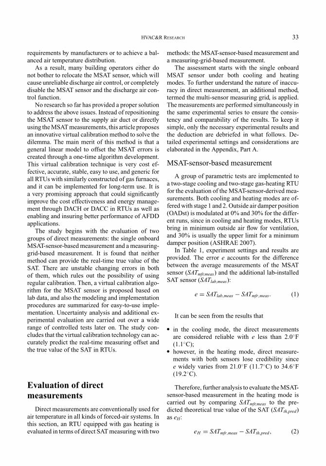
In Table 1, experiment settings and results areprovided. The error e accounts for the differencebetween the average measurements of the MSATsensor (SATmfr,meas) and the additional lab-installedSAT sensor (SATlab,meas):

e = SATlab,meas − SATmfr,meas. (1)

It can be seen from the results that

� in the cooling mode, the direct measurementsare considered reliable with e less than 2.0◦F(1.1◦C);

� however, in the heating mode, direct measure-ments with both sensors lose credibility sincee widely varies from 21.0◦F (11.7◦C) to 34.6◦F(19.2◦C).

Therefore, further analysis to evaluate the MSAT-sensor-based measurement in the heating mode iscarried out by comparing SATmfr,meas to the pre-dicted theoretical true value of the SAT (SATth,pred)as eH:

eH = SATmfr,meas − SATth,pred, (2)

Tab

le1.

Eva

luat

ion

ofM

SA

Tse

nsor

-bas

edm

easu

rem

entu

nder

both

cool

ing

and

heat

ing

mod

es.

Run

ning

mod

eR

unni

ngst

age

OA

Dst

Sce

nari

oID

SAT

lab,

mea

s(◦

F(◦

C))

SAT

mfr

,mea

s(◦

F(◦

C))

e(◦

F(◦

C))

Coo

ling

20%

C-1

48.2

(9.0

)46

.2(7

.9)

2.02

(1.1

)C

ooli

ng2

0%C

-238

.8(3

.8)

36.8

(2.7

)2.

0(1

.1)

Coo

ling

230

%C

-351

.2(1

0.7)

49.4

(9.7

)1.

8(1

.0)

Coo

ling

230

%C

-450

.4(1

0.2)

48.4

(9.1

)1.

9(1

.1)

Coo

ling

10%

C-5

62.3

(16.

8)61

.3(1

6.3)

1.0

(0.6

)C

ooli

ng1

0%C

-656

.4(1

3.6)

55.8

(13.

2)0.

5(0

.3)

Coo

ling

130

%C

-766

.4(1

9.1)

65.9

(18.

8)0.

5(0

.3)

Coo

ling

130

%C

-866

.0(1

8.9)

64.6

(18.

1)1.

4(0

.8)

Run

ning

mod

eR

unni

ngst

age

OA

Dst

Sce

nari

oID

SAT

lab,

mea

s

(◦F

(◦C

))SA

Tm

fr,m

eas

(◦F

(◦C

))

• Vm

eas(

cfm

(m3 /s

))SA

Tth

,pre

d

(◦F

(◦C

))M

AT

(◦F

(◦C

))e H

(◦F

(◦C

))e

(◦F

(◦C

))

Hea

ting

20%

H-1

151.

4(6

6.3)

120.

1(4

8.9)

1848

(0.8

7)10

8.0

(42.

2)54

.2(1

2.3)

12.1

(6.7

)31

.3(1

7.4)

Hea

ting

20%

H-2

151.

3(6

6.3)

120.

0(4

8.9)

2045

(0.9

7)10

8.3

(42.

4)59

.5(1

5.3)

11.7

(6.5

)31

.3(1

7.4)

Hea

ting

20%

H-3

152.

5(6

6.9)

121.

5(4

9.7)

1857

(0.8

8)10

8.9

(42.

7)55

.4(1

3.0)

12.6

(7.0

)31

.0(1

7.2)

Hea

ting

20%

H-4

155.

1(6

8.4)

124.

0(5

1.1)

1829

(0.8

6)11

1.8

(44.

3)57

.4(1

4.1)

12.2

(6.8

)31

.1(1

7.3)

Hea

ting

230

%H

-513

4.4

(56.

9)99

.9(3

7.7)

2076

(0.9

8)93

.0(3

3.9)

44.9

(7.2

)6.

9(3

.8)

34.5

(19.

2)H

eati

ng2

30%

H-6

138.

5(5

9.2)

104.

5(4

0.3)

2269

(1.0

7)96

.7(3

5.9)

52.5

(11.

4)7.

8(4

.3)

34.1

(18.

9)H

eati

ng2

30%

H-7

140.

5(6

0.3)

106.

1(4

1.2)

2037

(0.9

6)99

.2(3

7.3)

50.2

(10.

1)7.

0(3

.9)

34.4

(19.

1)H

eati

ng2

30%

H-8

144.

4(6

2.4)

109.

9(4

3.3)

2040

(0.9

6)10

2.7

(39.

3)53

.8(1

2.1)

7.2

(4.0

)34

.6(1

9.2)

Hea

ting

10%

H-9

120.

4(4

9.1)

99.4

(37.

4)18

53(0

.87)

94.7

(34.

8)59

.3(1

5.2)

4.6

(2.6

)21

.1(1

1.7)

Hea

ting

10%

H-1

011

9.1

(48.

4)98

.1(3

6.7)

2051

(0.9

7)93

.2(3

4.0)

61.0

(16.

1)4.

9(2

.7)

21.0

(11.

7)H

eati

ng1

0%H

-11

122.

1(5

0.1)

100.

8(3

8.2)

1849

(0.8

7)96

.4(3

5.8)

60.9

(16.

1)4.

3(2

.4)

21.4

(11.

9)H

eati

ng1

0%H

-12

124.

1(5

1.2)

102.

6(3

9.2)

1831

(0.8

6)99

.6(3

7.6)

63.7

(17.

6)3.

0(1

.7)

21.4

(11.

9)H

eati

ng1

30%

H-1

310

6.1

(41.

2)82

.6(2

8.1)

2081

(0.9

8)80

.4(2

6.9)

48.6

(9.2

)2.

2(1

.2)

23.5

(13.

1)H

eati

ng1

30%

H-1

410

6.4

(41.

3)83

.2(2

8.4)

2272

(1.0

7)82

.1(2

7.8)

52.9

(11.

6)1.

0(0

.6)

23.3

(12.

9)H

eati

ng1

30%

H-1

511

1.0

(43.

9)87

.5(3

8.3)

2059

(0.9

7)85

.5(2

9.7)

53.4

(11.

9)2.

0(1

.1)

23.5

(13.

1)H

eati

ng1

30%

H-1

611

4.8

(46.

0)90

.8(3

2.7)

2046

(0.9

7)88

.7(3

1.5)

56.4

(13.

6)2.

1(1

.2)

24.0

(13.

3)

34

HVAC&R RESEARCH 35

where SATth,pred is derived from an energy balance,shown as Equation 3:

SATth,pred =•Q H

CP ו

V meas

v +MAT+�T f an, (3)

where•Q H is the heating capacity in Btu/hr (kJ/s),

•V meas is the measured supply air flow rate in cfm(m3/s), CP is the specific heat at constant pressurein Btu/(lbm◦F) (kJ/(kg·K)), v is the specific volumeof air in lb/ft3 (m3/kg), MAT is the MAT before thegas burner in ◦F (◦C), and �Tfan is the supply fantemperature rise in ◦F (◦C).

The procedures of measuring the parameters inEquations 1–3 are addressed in detail in the Ap-pendix, Part A. As given in Table 1, eH is found tobe unstable with the MSAT-sensor-based measure-ment. It alters in a wide range from 1.0◦F (0.6◦C)to 12.6◦F (7.0◦C) when test condition varies. It isobviously improper to directly use SATmfr,meas in theheating mode as the true value of the SAT in theRTU. The results also demonstrate that a regularcalibration with a fixed offset based on the MSAT-sensor-based direct measurement would fail.

Measuring-grid-based measurement

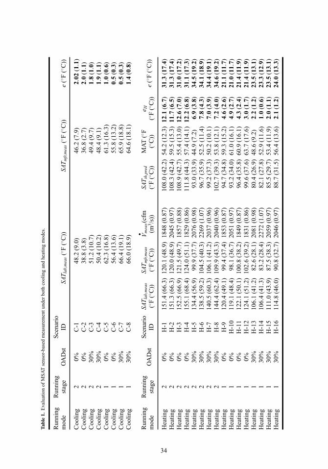
A measuring grid in the inlet of the supply airduct and right out of the RTU is also constructedfor the experiments. Since the grid is not located inthe chamber, the radiation influence from the gasburner can be attenuated to some extent. The multi-point measurements employed in a measuring gridare also supposed to improve the overall measure-ment accuracy with less stratification impact. Eighttemperature sensors are positioned in the duct workafter the RTU, as depicted in Figure 1. With eightsensors, the duct section representative locations arewell covered.

Average values of each sensor from 1 to 8 (SATG,C

for the cooling mode and SATG,H for the heatingmode); the MSAT-sensor-based SATmfr,meas and thecalculated SATth,pred are plotted in Figure 2 for com-parison. The horizontal axis is for different sensorID, and the vertical axis is for air temperatures inFahrenheit and Celsius degrees. To get a clear view,the results of all cooling scenarios and half of the16 heating scenarios are given in Figure 2.

The results of the cooling mode illustrate that themeasurements of eight SATG,C are close to those ofSATmfr,meas. In all cooling scenarios, the error be-

Figure 1. Illustration of measuring grid and numbered sensors.

tween the mean of eight SATG,C and SATmfr,meas isabout 1.5◦F (0.8◦C) or less. It is consistent with theprevious evaluation for the MSAT-sensor-based di-rect measurement. Both the MSAT sensor and themeasuring grid in the cooling mode are trustworthyfor use.

From the heating mode plot, the following pointscan be observed:

� Temperature distribution of eight SATG,H is irreg-ular: Combining Figures 1 and 2, the relationshipsof eight SATG,H and their location in the heatingmode are erratic. Temperature values of sensors1 to 4 are lower than those of the correspondingsensors 5 to 8. It is unsuitable to calculate the truevalue of the SAT by averaging eight SATG,H.

� A big temperature difference exists betweenSATmfr,meas and the average eight SATG,H: In sce-nario H-7, for example, SATmfr,meas is 106.1◦F(41.2◦C); SATG,H sensors 1 to 8 give the low-est reading as 74.4◦F (23.6◦C) and the highest as108.7◦F (42.6◦C). It makes the differential tem-perature between SATmfr,meas and the average eightSATG,H 8.9◦F (4.9◦C). In all heating scenarios,the error between SATmfr,meas and the mean ofeight SATG,H varies from 3.0◦F (1.7◦C) to 12.2◦F(6.8◦C).

� Various temperature difference stands betweenSATth,pred and the mean of eight SATG,H:The temperature difference between SATth,pred

and the mean of eight SATG,H varies in differentscenarios. For example, in scenario H-7, with

36 VOLUME 17, NUMBER 1, 2011

Figure 2. Evaluation of measuring grid under both cooling and heating modes: (a) IP units and (b) SI units.

heating stage (Hstage) 2 and OADst 30%, themean of eight SATG,H is 95.2◦F (35.1◦C) whilethe true value SATth,pred is 99.2◦F (37.3◦C) (with4.0◦F [2.2◦C] temperature difference). However,in scenario H-16 with Hstage 1 and OADst 30%,the mean of eight SATG,H is 85.9◦F (29.9◦C) whilethe true value SATth,pred is 88.7◦F (31.5◦C) (with2.8◦F [1.6◦C] temperature difference). As pre-sented in this case, the measuring grid does notindicate the true value of the SAT.

In summary, the evaluation of the measuring gridfurther testifies that the offset error for the MSATin heating mode varies. Controls in RTUs relatedto MSAT sensor direct measurements in the heatingmode can be far from the intended operation andlead to inferior system performance. In addition,using the measuring grid does not help obtain thetrue value of the SAT in RTUs. It also could not be

used for the verification of the predicted true valueof the SAT. An innovative calibration algorithm isneeded to fill in the gap.

Algorithm development andimplementation issues

Algorithm development

As analyzed above, direct measurement, eitherthe single MSAT-sensor-based or the measuring-grid-based, cannot catch the true value of the SAT.The measuring-grid method in a location out of theRTU merely provides a closer but still mediocreprediction. Besides, additional construction, costs,maintenance, and sources for uncertainty areincurred by using the measuring grid. It is not apractical tool in real applications.

HVAC&R RESEARCH 37

Figure 3. eH vs OADst in different Hstage: (a) IP units and (b)SI units.

Variables in the experiments are thus reinvesti-gated to identify the algorithm that might be usefulto predict the offset for the calibration of the MSAT-sensor-based measurement.

As shown in Figure 3, error eH is a strong functionof Hstage and OADst. A liner model can be fitted torepresent the relationship between eH, Hstage, andOADst in RTUs. As shown in Equation 4, the modelcan be used to estimate the calibration error (ecal) ofthe MSAT sensor under certain Hstage and OADst;verification through more lab tests is explored inlater sections:

ecal = a + b × Hstage+ c × Hstage2

+ d × OADst + f × OADst2

+ g × Hstage× OADst. (4)

Once such an offset ecal expression is obtained fora given type of RTU, it can be utilized to correct the

MSAT-sensor-based measurement for the true valuein RTUs. The equation for the calibrated MSATsensor (SATmfr,cal) is given below:

SATmfr,cal = SATmfr,meas − ecal . (5)

For this 7.5-ton rooftop unit with 130,000 Btu/hr(38.1 kW) gas heating capacity, the coefficients forthe linear model are obtained with the experimentaldata. The results are listed in Table 2, with R-square0.98.

Equations 4 and 5 jointly constitute the modelof the virtual calibration that can be directly trans-planted to different RTUs.

Implementation issues

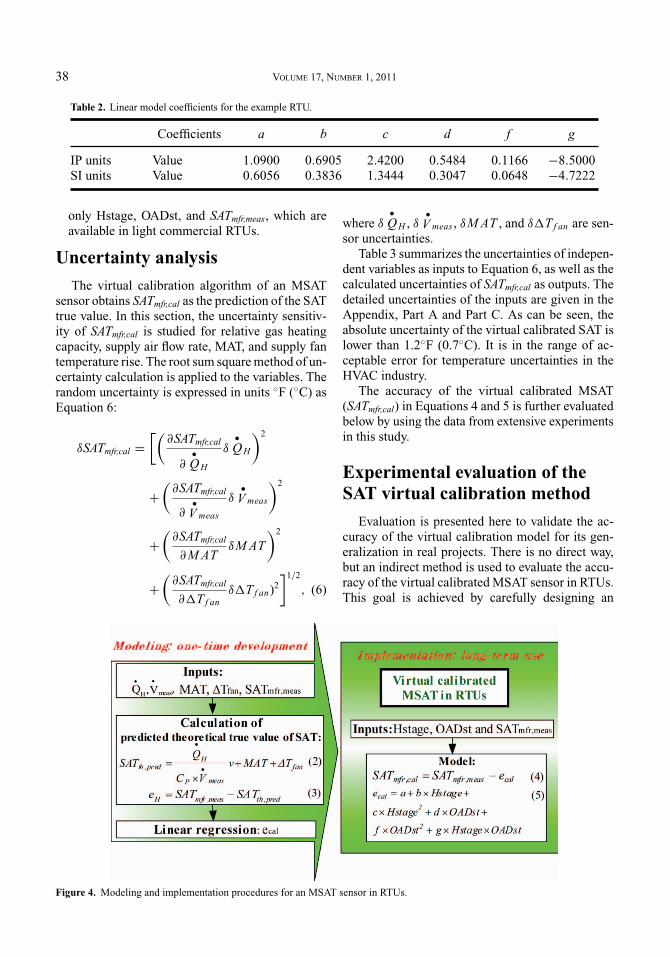
With the analysis of SAT direct measurementsand algorithm development of the virtual calibrationfor an MSAT sensor presented above, a summary ofimplementation issues, including the procedures ofa one-time model development and its implemen-tation for long-term use in RTUs, can be given, asillustrated in Figure 4.

� One-time development: According to Equations2 and 3, the measurements and inputs for the pro-cedure of algorithm development are SATmfr,meas,•Q H ,

•V meas , MAT, and �Tfan. SATmfr,meas is the

measurement of an MSAT sensor.•Q H can be re-

ferred to manufacturers’ information.•

V meas canbe obtained with the test and balance when theRTUs are installed at the beginning or measuredthrough a one-time test. �Tfan can be calculatedby using the way proposed by Wichman andBraun (2009). MAT is estimated using the ap-proaches provided by Yang and Li (2010). Thereader can refer to the Appendix, Part A, whichexplains these parameters in detail.The correlated virtual calibration model for thebias errors of an MSAT sensor is needed only onceand generic for all RTUs with similar constructionof gas furnaces.

� Long-term use: Once the one-time developmentis conducted, the implementation of virtual cali-bration for long-term use is ready and easy withthe otherwise unpredictable errors under differentoperations. According to Equations 4 and 5, themeasurements and inputs for long-term use are

38 VOLUME 17, NUMBER 1, 2011

Table 2. Linear model coefficients for the example RTU.

Coefficients a b c d f g

IP units Value 1.0900 0.6905 2.4200 0.5484 0.1166 −8.5000SI units Value 0.6056 0.3836 1.3444 0.3047 0.0648 −4.7222

only Hstage, OADst, and SATmfr,meas, which areavailable in light commercial RTUs.

Uncertainty analysis

The virtual calibration algorithm of an MSATsensor obtains SATmfr,cal as the prediction of the SATtrue value. In this section, the uncertainty sensitiv-ity of SATmfr,cal is studied for relative gas heatingcapacity, supply air flow rate, MAT, and supply fantemperature rise. The root sum square method of un-certainty calculation is applied to the variables. Therandom uncertainty is expressed in units ◦F (◦C) asEquation 6:

δSATmfr,cal =[(

∂SATmfr,cal

∂•Q H

δ•Q H

)2

+(

∂SATmfr,cal

∂•

V meas

δ•

V meas

)2

+(

∂SATmfr,cal

∂ M ATδM AT

)2

+(

∂SATmfr,cal

∂�T f anδ�T f an)2

]1/2

, (6)

where δ•Q H , δ

•V meas , δM AT , and δ�T f an are sen-

sor uncertainties.Table 3 summarizes the uncertainties of indepen-

dent variables as inputs to Equation 6, as well as thecalculated uncertainties of SATmfr,cal as outputs. Thedetailed uncertainties of the inputs are given in theAppendix, Part A and Part C. As can be seen, theabsolute uncertainty of the virtual calibrated SAT islower than 1.2◦F (0.7◦C). It is in the range of ac-ceptable error for temperature uncertainties in theHVAC industry.

The accuracy of the virtual calibrated MSAT(SATmfr,cal) in Equations 4 and 5 is further evaluatedbelow by using the data from extensive experimentsin this study.

Experimental evaluation of theSAT virtual calibration method

Evaluation is presented here to validate the ac-curacy of the virtual calibration model for its gen-eralization in real projects. There is no direct way,but an indirect method is used to evaluate the accu-racy of the virtual calibrated MSAT sensor in RTUs.This goal is achieved by carefully designing an

Figure 4. Modeling and implementation procedures for an MSAT sensor in RTUs.

Tab

le3.

Unc

erta

inty

anal

ysis

ofSA

Tm

fr,c

al.

Inde

pend

entv

aria

bles

Inpu

tsU

ncer

tain

ty

Gas

heat

ing

capa

city

,• Q

H(B

tu/h

r(k

W))

Hst

age

1:84

,500

(24.

8)±2

%H

stag

e2:

130,

000

(38.

1)

Mea

sure

dsu

pply

air

flow

rate

,• Vm

eas,

(cfm

(m3 /s

))D

efau

ltda

tain

Tabl

e1

±1%

MA

T(◦

F(◦

C))

Def

ault

data

inTa

ble

1±1

.0◦ F

(0.6◦ C

)S

uppl

yfa

nte

mpe

ratu

reri

se,�

Tfa

n(◦

F(◦

C))

1.7◦

F(0

.9◦ C

)±0

.2◦ F

(0.1◦ C

)

Dep

ende

ntva

riab

leC

alib

rate

dm

anuf

actu

rer-

inst

alle

dS

AT

sens

or,S

AT

mfr

,cal

(◦F

(◦C

))S

cena

rio

IDH

-1H

-2H

-3H

-4H

-5H

-6H

-7H

-8U

ncer

tain

ty(◦

F)

1.2

(0.7

)1.

1(0

.6)

1.2

(0.7

)1.

2(0

.7)

1.1

(0.6

)1.

1(0

.6)

1.1

(0.6

)1.

1(0

.6)

Sce

nari

oID

H-9

H-1

0H

-11

H-1

2H

-13

H-1

4H

-15

H-1

6U

ncer

tain

ty(◦

F)

1.1(

0.6)

1.1(

0.6)

1.1(

0.6)

1.1(

0.6)

1.1(

0.6)

1.1(

0.6)

1.1(

0.6)

1.1(

0.6)

39

40 VOLUME 17, NUMBER 1, 2011

Figure 5. The experiment evaluation procedures of the virtual calibration methodology.

experiment in a laboratory environment. The de-tailed experiment configuration and analysis aregiven in the Appendix, Part A and Part B.

Evaluation layout

Figure 5 depicts the experiment evaluation pro-cedures of the virtual calibration methodology pre-sented in this article. The idea of using energybalance under both cooling (forward) and heating(backward) mode is innovatively conducted.

The verification is implemented by comparingSATmfr,cal in Equation 4 to experimentally calculatethe true value of SAT (SATexp,eva). SATexp,eva is ob-tained based on an energy balance of the heat lossthrough the duct work. It is a counterpart of SATmfr,cal

but is used for evaluation purposes only. To calculateSATexp,eva, the knowns and assumptions are listed asfollows:

� The mean of eight SATG,C is regarded as the truevalue of the SAT in the cooling mode.

� Measurements of six air temperature sensors atthe supply air duct outlet are reliable under boththe heating (SATO,H) and cooling modes (SATO,C).The average of six SATO,H and the average of sixSATO,C are used in the calculation. The supportiveanalysis of these temperatures is presented in theAppendix, Part B.

� UA of the supply air duct work from the measur-ing grid to the outlet is assumed to be constantunder both cooling and heating modes.

� Supply air flow rate (•

V meas) and additional tem-perature measurements are taken in the locationwhere the air is well mixed.

Evaluation implementation

Three main steps of evaluation in sequence areincluded as follows.

Step 1: Correcting UA in cooling mode. Heat lossin the cooling mode (Qloss,C) through the ductwork leads to the air temperature change from themeasuring grid cross-section to the outlet in theduct. Heat transfer surface (A) and heat transfercoefficient (U) of the duct work are constants;

therefore, UA could be deduced with•

V meas , OAT,SATG,C, and SATO,C.

Step 2: Correlating SATexp,eva. Similarly, SATexp,eva

in the heating mode should be acquired while

UA,•

V meas , SATO,H, and OAT are known.Step (3): Verification of SATmfr,cal

Finally, SATmfr,cal in heating mode is evaluatedafter SATexp,eva is derived from experiments.

Correcting UA in cooling modeThe goal here is to estimate the constant UA in

the lab environment with the data points collectedin the experiment series in cooling mode. To inves-tigate the UA, it is assumed that (1) the overall heattransfer coefficient is constant, (2) the specific heatof air is constant, and (3) the supply air flow rate isconstant because a fixed-fan speed is incorporatedin the RTU.

HVAC&R RESEARCH 41

Table 4. Correcting UA in cooling mode.

Scenario ID

•Vmeas

(cfm (m3/s))SATO,C

(◦F (◦C))SATG,C

(◦F (◦C))OAT

(◦F (◦C))Qloss,C

(Btu/hr(kW))�TC

(◦F (◦C))

C-1 1931 (0.9) 49.4 (9.7) 48.0 (8.9) 81.8 (27.7) 2982 (0.87) 33.1 (18.4)C-2 2328 (1.1) 41.1 (5.1) 38.6 (3.7) 87.8 (31.0) 6311 (1.85) 47.9 (26.6)C-3 2084 (1.0) 52.3 (11.3) 51.1 (10.6) 82.3 (27.9) 2566 (0.75) 30.6 (17.0)C-4 2595 (1.2) 51.9 (11.1) 50.3 (10.2) 87.0 (30.6) 4596 (1.35) 35.9 (19.9)C-5 1874 (0.9) 63.0 (17.2) 62.5 (16.9) 79.6 (26.4) 1154 (0.34) 16.9 (9.4)C-6 2251 (1.1) 58.5 (14.7) 57.0 (13.9) 81.8 (27.7) 3792 (1.11) 24.1 (13.4)C-7 2026 (1.0) 66.5 (19.2) 66.0 (18.9) 81.9 (27.7) 1094 (0.32) 15.7 (8.7)C-8 2526 (1.2) 68.2 (20.1) 67.4 (19.7) 86.4 (30.2) 2373 (0.70) 18.7 (10.3)

In the cooling mode, with•

V meas , OAT, SATG,C,and SATO,C known, Qloss,C can be calculated:

Qloss,C =•

V meas × C p × (SATO,C − SATG,C )

v.

(7)Meanwhile, Qloss,C also can be expressed as

Qloss,C = UA

(OAT− SATO,C + SATG,C

2

). (8)

Combining the two expressions gives

•V meas × C p × (SATO,C − SATG,C )

v

= UA

(OAT− SATO,C + SATG,C

2

). (9)

Put variable �TC as follows:

�TC = OAT− SATO,C + SATG,C

2.

So, Equation 9 can be further simplified to theequation below:

Qloss,C = UA�TC . (10)

Eight sets of•

V meas , OAT, SATG,C, and SATO,C, aswell as the intermediate value Qloss,C and �TC, arelisted in Table 4.

Figure 6 shows that Qloss,C and �TC have a pos-itive linear correlation. Data points scatter closelybeside a line. The slope of the linear-regressed line,which is 115.47, can be used as the value of UAfor the duct work. In other words, UA is foundas 115.47 Btu/hr ◦F (0.06 kW/K). As a physical

Figure 6. UA linear regression: (a) IP units and (b) SI units.

42 VOLUME 17, NUMBER 1, 2011

Table 5. Results of evaluation of SATmfr,cal.

Scenario IDSATexp,eva

(◦F (◦C))V̇meas

(cfm (m3/s))SATmfr,cal

(◦F (◦C)) eeva (◦F (◦C))

H-1 108.6 (42.6) 1848 (0.87) 108.0 (42.2) –0.6 (–0.3)H-2 108.8 (42.7) 2045 (0.97) 108.3 (42.4) –0.5 (–0.3)H-3 110.1 (43.4) 1857 (0.88) 108.9 (42.7) –1.1 (–0.6)H-4 112.3 (44.6) 1829 (0.86) 111.8 (44.3) –0.5 (–0.3)H-5 92.4 (33.6) 2076 (0.98) 93.0 (33.9) 0.6 (0.3)H-6 95.9 (35.5) 2269 (1.07) 96.7 (35.9) 0.7 (0.4)H-7 98.4 (37.3) 2037 (0.96) 99.2 (37.3) 0.7 (0.4)H-8 101.9 (39.3) 2040 (0.96) 102.7 (39.3) 0.8 (0.4)H-9 95.2 (35.1) 1853 (0.87) 94.7 (34.8) –0.5 (–0.3)H-10 93.9 (34.4) 2051 (0.97) 93.2 (34.0) –0.6 (–0.3)H-11 96.7 (35.9) 1849 (0.87) 96.4 (35.8) –0.3 (–0.2)H-12 98.8 (37.1) 1831 (0.86) 99.6 (37.6) 0.8 (0.4)H-13 80.8 (27.1) 2081 (0.98) 80.4 (26.9) –0.4 (–0.2)H-14 81.1 (27.3) 2272 (1.07) 82.1 (27.8) 1.0 (0.6)H-15 85.5 (29.7) 2059 (0.97) 85.5 (29.7) 0.0 (0.0)H-16 88.9 (31.6) 2046 (0.97) 88.7 (31.5) –0.2 (–0.1)

characteristic of the duct work, this value remainsunchanged when gas heating is operating.

Correlating SATexp,eva

As pointed out previously, with UA,•

V meas ,SATO,H, and the OAT known, SATexp,eva could beobtained by jointly solving Equations 11 and 12:

Qloss,H =•

V meas × C p × (SATexp,eva − SATO,H )

v,

(11)

Qloss,H = UA

(OAT− SATexp,eva + SATO,H

2

).

(12)The results of SATexp,eva are summarized in Ta-

ble 5. From this point on, SATexp,eva can be used toevaluate the accuracy of SATmfr,cal.

Evaluation of SATmfr,calTo estimate the accuracy of SATmfr,cal, the error

eeva between SATmfr,cal and SATexp,eva given as Equa-tion 13 is to be analyzed:

eeva = SATmfr,cal − SATexp,eva . (13)

The results are compiled in Table 5. The erroreeva is within the range of ±1.1◦F (0.6◦C). Thus,

SATmfr,cal is demonstrated to be credible and can betrusted as the true value of the SAT in RTUs.

Conclusions and discussion

The single MSAT-sensor-based direct measure-ment is conventionally used in RTUs to obtain theSAT. But the accuracy and reliability is greatly com-promised in the heating mode due to severe temper-ature stratification and high thermal radiation. Thesingle onboard MSAT-sensor- and measuring-grid-based measurements are evaluated through a set oftests in a lab. The experiments are designed to coverrepresentative operations in both cooling and heat-ing modes. It is found that, although direct measure-ments have reasonably good accuracy in the coolingmode, there are unacceptable erratic errors in theheating mode and a regular calibration can hardlyovercome the defect.

An easy-to-use virtual calibration methodologyis then proposed. A general linear model relying onavailable operation information is derived to acquirethe various offsets. Further, experimental evaluationand uncertainty analysis are conducted to prove theperformance of this innovative method. The studyindicates that the virtual calibration of an MSATsensor in RTUs:

� is robust enough against various operating condi-tions,

HVAC&R RESEARCH 43

� has very good accuracy (the uncertainty is±1.2◦F[0.7◦C]),

� is easy to implement and economical for use, and� is generic for all RTUs with similar construction

of gas furnaces.

For SAT-based sequencing control in RTUs, im-proved energy efficiency and higher reliability couldbe achieved by using accurate measurements of avirtually calibrated MSAT sensor. Knowledge of theSAT true value in RTUs will also benefit real-timeautomated control, AFDD, and other advance appli-cations. For instance,

� it could serve as part of a permanently installedcontrol or monitoring system to ensure accuracyin SAT measurement;

� it could help find the Hstage failure fault in RTUsby evaluating the differential temperature acrossthe gas furnaces; and

� it also could be utilized to develop a virtual sup-ply airflow rate meter, which is important formonitoring, controlling, diagnosing, and optimiz-ing indoor air quality and energy consumption inRTUs.

In this study, only RTUs with constant air vol-ume (CAV) application are considered. However,variable air volume (VAV) becomes more and morepopular in large commercial RTUs with a capacitylarger than 30 tons. It is anticipated that the methodcould be adopted for VAV RTU systems used inlarger commercial buildings. It could be a topic forfuture studies.

Nomenclature

A = heat transfer area, ft2 (m2)AFDD = automated fault detection and diagno-

sisCa = fluid capacity rate of air side,

Btu/(hr·◦F) (kW/K)CAV = constant air volumeCg = fluid capacity rate of gas side,

Btu/(hr·◦F) (kW/K)CP = specific heat capacity at constant pres-

sure, Btu/(lbm·◦F) (kJ/(kg·K))e = error between SATlab,meas and

SATmfr,meas, ◦F (◦C)DACC = discharge (supply) air control of cool-

ingDACH = discharge (supply) air control of heat-

ing

DOE = Department of EnergyEAT = exhaust air temperature, ◦F (◦C)ecal = offset error for calibration of the

manufactured-installed supply airtemperature sensor, ◦F (◦C)

eH = error between SATth,pred andSATmfr,meas, ◦F (◦C)

eeva = error between SATmfr,cal andSATexp,eva, ◦F (◦C)

Hstage = gas heating stage•m = mass flow rate, lb/hr (kg/s)MAT = mixed air temperature, ◦F (◦C)MSAT = measured manufacturer-installed sup-

ply air temperatureNTU = number of transfer unitsOADst = outside air damper positionOAT = outside air temperature, ◦F (◦C)•Q H = gas heating capacity, Btu/hr (kW)Qloss,C = heat loss in the supply air duct in cool-

ing mode, Btu/hr (kW)Qloss,H = heat loss in the supply air duct in heat-

ing mode, Btu/hr (kW)r = outside fresh air ratioRTU = rooftop air conditioning unitRAT = return air temperature, ◦F (◦C)SAT = supply air temperature, ◦F (◦C)SATexp,eva = indirect experimentally calculated

true value of SAT, ◦F (◦C)SATG,C = measured SAT of the measuring grid

in cooling mode, ◦F (◦C)SATG,H = measured SAT of the measuring grid

in heating mode, ◦F (◦C)SATlab,meas = measured SAT with lab-installed tem-

perature sensor, ◦F (◦C)SATmfr,cal = calibrated SAT for the manufacturer-

installed temperature sensor, ◦F (◦C)SATmfr,meas = measured SAT with manufacturer-

installed temperature sensor, ◦F (◦C)SATO,C = measured SAT at the outlet of supply

air duct in cooling mode, ◦F (◦C)SATO,H = measured SAT at the outlet of supply

air duct in heating mode, ◦F (◦C)SATO,lab = measured SAT with lab-installed sen-

sor at the outlet of supply air duct, ◦F(◦C)

SATth,pred = predicted theoretical true value ofSAT, ◦F (◦C)

U = heat transfer coefficient, Btu/(hr·◦F·ft2) (kW/(m2·K))

•V C = calculated supply air flow rate, cfm

(m3/s)

44 VOLUME 17, NUMBER 1, 2011

•Vmeas = measured supply air flow rate, cfm

(m3/s)�Tfan = temperature rise across the supply fan,

◦F (◦C)v = specific volume of air, ft3/lbm (m3/kg)VAV = variable air volumeε = heat exchanger effectivenessρa = air density, lb/ft3 (kg/m3)

Subscripts

a = airC = coolingcal = calibrationd = designeva = evaluationexp = experimentalfan = supply air fang = gasG = gridH = heatingI = inletlab = lab-installedloss = heat lossmax = maximummeas = measuredmfr = manufacturermin = minimumo = outletO = outlet of supply air ductP = constant pressurepred = predictedth = theoreticalven = ventilation

ReferencesASHRAE. 2007. ASHRAE Standard 62.1-2007, Ventilation for

Acceptable Indoor Air Quality. Atlanta, GA: American So-ciety of Heating, Refrigerating and Air-conditioning Engi-neers, Inc.

ASHRAE. 2009. 2009 ASHRAE Handbook—Fundamentals. At-lanta, GA: American Society of Heating, Refrigerating andAir-Conditioning Engineers, Inc.

ASME. 1974. ANSI/ASME Standard PTC 19.3-1974 (R1998),Temperature measurement instruments and apparatuss. NewYork: American Society of Mechanical Engineers.

Breuker, M.S. 1997. Evaluation of a statistical, rule-based faultdetection and diagnostics method for vapor compression airconditioners. Master’s thesis, School of Mechanical Engi-neering, Purdue University, West Lafayette, Indiana.

Breuker, M.S., and J.E. Braun. 1998a. Common faults and theirimpacts for rooftop air conditioners. International Journal

of Heating, Ventilating, Air Conditioning and RefrigeratingResearch 4(3):303–18.

Breuker, M.S., and J.E. Braun. 1998b. Evaluating the perfor-mance of a fault detection and diagnostic system for va-por compression equipment. International Journal of Heat-ing, Ventilating, Air Conditioning and Refrigerating Research4(4):401–25.

Katipamula, S., and M.R. Brambley. 2005. Methods for fault de-tection, diagnostics, and prognostics for building systems—areview, Part I. HVAR&R Research 11(1):3–25.

Lennox. 2007. M1-7 Version 5.02 integrated modular controller(IMC). Dallas, TX: Lennox Technical Publication.

Li, H., and J.E. Braun. 2003. An improved method for faultdetection and diagnosis applied to packaged air conditioners.ASHRAE Transactions 109(2):683–92.

Li, H., and J.E. Braun. 2007a. A methodology for diagnosingmultiple-simultaneous faults in vapor compression air con-ditioners. HVAS&R Research, 13(2):369–95.

Li, H., and J.E. Braun. 2007b. Decoupling features and virtualsensors for diagnosis of faults in vapor compression air con-ditioners. International Journal of Refrigeration 30(3):546–64.

Li, H., and J.E. Braun. 2007c. An overall performance indexfor characterizing the economic impact of faults in directexpansion cooling equipment. International Journal of Re-frigeration 30(2):299–310.

Parmelee, G.V., and R.G. Huebscher. 1946. The shielding ofthermocouples from the effects of radiation. ASHRAE Trans-actions 52:183.

Rossi, T.M. 1995. Detection, diagnosis, and evaluation of faults invapor compression cycle equipment. Ph.D. thesis, School ofMechanical Engineering, Purdue University, West Lafayette,Indiana.

Rossi, T.M., and J.E. Braun. 1997. A statistical, rule-based faultdetection and diagnostic method for vapor compression airconditioners. International Journal of Heating, Ventilating,Air Conditioning and Refrigerating Research 3(1):19–37.

Westphalen, D., and S. Koszalinski. 2001. Energy consumptioncharacteristics of commercial building HVAC systems: Vol-ume I—chillers, refrigerant compressors, and heating sys-tems. Final Report to the U.S. Department of Energy, Wash-ington, DC (Contract No. DE-AC01-96CE23798).

Wichman, A., and J.E. Braun. 2009. A smart mixed-air temper-ature sensor. HVAR&R Research 15(1):101–15.

Yang, M., and H. Li. 2011. A virtual outside air ratio in packagedair conditioners. HVAC&R Research (forthcoming).

Appendix

Part A—experiment configuration

Sixteen heating experiments for assessment ofdirect measurements and indirect calculations of theSAT are performed in a lab with two artificial cli-mate chambers. For evaluation purposes, an addi-tional eight experiments in the cooling mode arealso carried out.

HVAC&R RESEARCH 45

Figure 7. Illustration of machine layout in the lab.

System descriptionA 7.5-ton RTU equipped with two constant-

speed compressors and a two-stage gas furnace witha 130,000 Btu/hr (38.1 kW) heating capacity com-poses the main experiment body (Figure 7). It sitsin the outdoor environmental chamber and controlsthe indoor chamber with conditioned air. The nom-inal supply air flow rate is 2400 cfm (1.13m3/s)with a standard speed option. Together with anotherRTU outside of the building, artificial indoor andoutdoor air physical conditions can be created andmaintained.

Measurements descriptionBesides the MSAT sensor, there are more than ten

additional important air temperature sensors as wellas supportive temperature definitions. The measure-ments and concepts indispensable to accomplish thestudy are listed in what follows.

OATSince the manufacturer-installed OAT sensor is

fixed beside the evaporator coils, improper heat gainand poor air distribution may affect the accuracyof the OAT measurements. Instead, a lab-installedOAT sensor mounted on the RTU outside the airinlet is used. The sensor, as are all other physicaltemperature sensors installed, has been calibratedwith a precision of ±0.5◦F (0.3◦C).

Measurement of lab-installed SAT sensorOne more SAT sensor is installed in the RTU

to supplement the measurement of SAT. The sen-sor is referred to as the lab-installed SAT sensor(SATlab,meas). The function is to verify and alsobackup the MSAT sensor in case of failure.

Supply fan temperature rise�Tfan is calculated using the heat loss from the

fan and is checked with actual measurements us-

ing the method presented by Wichman and Braun(2009) under conditions where neither mechanicalcooling nor heating is operating.

The result of �Tfan in this article is 1.7◦F (0.9◦C)with an uncertainty of ±0.2◦F (0.1◦C). Since it isa CAV RTU, the uncertainty of the fan temperaturerise is relatively small.

MATAccurate direct MAT measurements are noto-

riously difficult to obtain in RTUs due to spaceconstraints and the use of small chambers for mix-ing outdoor and return air (ASME 1974). Muchresearch has been conducted to indirectly obtain theaccurate MAT measurements in RTUs. For exam-ple, Wichman and Braun (2009) proposed a smartMAT sensor for packaged systems that self-correctsthe errors and accurately estimates the MAT us-ing only a single-point measurement of MAT bycorrelating the errors with damper position signalsand the temperature difference between outdoorand return air. Extensive lab testing demonstratesthat the smart MAT sensor performs very well,and the overall root-mean-squared error is 0.57◦F(0.3◦C).

However, a physical MAT sensor is not typicallyinstalled in light commercial RTUs due to its badperformance, so this smart MAT sensor cannot beimplemented without adding a new MAT sensor. Tofurther simplify this technique, Yang and Li (2010)proposed an alternative method that eliminates theneed of a physical MAT sensor and instead con-structs a virtual MAT sensor to estimate MAT usingdamper position signals, OAT, RAT, and a calibratedvirtual outdoor air ratio sensor. Both laboratory andfield testing demonstrate an acceptable uncertaintyof ±1.0◦F (0.6◦C). Since there is no pre-installedphysical MAT sensor available in this study, the lat-ter method was adopted.

46 VOLUME 17, NUMBER 1, 2011

Figure 8. Sensors layout of additional six air temperaturesensors.

Supply air flow rateAn air flow rate meter offering ±1% full-scale

accuracy is mounted in the supply air duct in the lab.It has been calibrated and verified by using anotherflow hood.

Measurements of the measuring grid sensorsAs presented previously, Figure 1 illustrates the

arrangement of the measuring-grid temperature sen-sors. Eight sensors are symmetrically mounted at thesupply air duct inlet.

Measurements of additional six air temperaturesensors

Figure 8 depicts the installation of six air tem-perature sensors at the supply air duct outlet to the

indoor chamber. Measurements under both the cool-ing (SATO,C) and the heating (SATO,H) modes ofthese six air temperature sensors are collected.

Measurement of lab-installed temperaturesensor at the supply air duct outlet

The sensor is referred to as a lab-installed temper-ature sensor at the supply air duct outlet (SATO,lab).The function is to verify the additional six tem-perature sensors at the supply air duct outlet inFigure 8.

Experiment settingsExperiment setups are collected in Table 6. To

cover most combinations, both cooling and heatingmodes are conducted with different running stages,OADst, and OAT. The OAT is kept low for the heat-ing mode and high for the cooling mode with rea-sonable distribution.

Each experiment assigned a scenario ID is con-ducted around 20 min for preparation, and followedby 10 to 15 min under steady status (Li and Braun2003). Instant readings for each sensor are sampledevery 15 s, and the mean of the samples is then usedto represent the corresponding measurement result.

Part B—evaluation of SATO,C and SATO,H

In the lab environment, the supply air duct isabout 3.5 m long, connecting the outdoor cham-ber and the indoor chamber. In order to carry outthe verification for this virtual calibration method,measurements of air temperature at the supplyair duct outlet with six sensors are evaluated un-der both cooling and heating modes (Figure 9).

Table 6. Lab experiment settings.

Runningmode

Runningstage OADst

OAT(◦F (◦C))

ScenarioID

Runningmode

Runningstage OADst

OAT(◦F (◦C))

ScenarioID

Heating 2 0% 36.0 (2.2) H-1 Heating 1 0% 35.6 (2.0) H-9Heating 2 0% 42.9 (6.1) H-2 Heating 1 0% 45.9 (7.7) H-10Heating 2 0% 44.1 (6.7) H-3 Heating 1 0% 44.4 (6.9) H-11Heating 2 0% 50.0 (10.0) H-4 Heating 1 0% 49.2 (9.6) H-12Heating 2 30% 34.4 (1.3) H-5 Heating 1 30% 34.1 (1.2) H-13Heating 2 30% 44.3 (6.8) H-6 Heating 1 30% 42.9 (6.1) H-14Heating 2 30% 43.3 (6.3) H-7 Heating 1 30% 43.1 (6.2) H-15Heating 2 30% 49.1 (9.5) H-8 Heating 1 30% 48.4 (9.1) H-16Cooling 2 0% 81.8 (27.7) C-1 Cooling 1 0% 79.6 (26.4) C-5Cooling 2 0% 87.8 (31.0) C-2 Cooling 1 0% 81.8 (27.7) C-6Cooling 2 30% 82.3 (27.9) C-3 Cooling 1 30% 81.9 (27.7) C-7Cooling 2 30% 87.0 (30.6) C-4 Cooling 1 30% 86.4 (30.2) C-8

HVAC&R RESEARCH 47

Figure 9. Evaluation of additional six temperature sensors under both cooling and heating modes: (a) IP units and (b) SIunits.

Measurements of another lab-installed sensor at thesupply air duct outlet (SATO,lab) are gathered for ref-erence.

In the cooling mode, the average error betweenSATO,lab and the mean of six SATO,C is less than 1◦F(0.6◦C). In the meantime, in the heating mode, theerror between SATO,lab and the mean of six SATO,C islower 3◦F (1.7◦C). As expected, at the cross-sectionclose to the outlet, air is well mixed and temperaturedistribution is fairly balanced. So in this study, themean of six SATO,C and the mean of six SATO,H areused in the verification process.

Part C—uncertainty analysis of heatingcapacity

Referring to ASHRAE Handbook—Fundamental(ASHRAE 2009; Chapter 4), for heat exchangers),to calculate the heating transfer rate, mean tem-perature difference analysis and number of transferunits (NTU)-effectiveness (ε) analysis are used. Theformer method involves trial-and-error calculations,unless inlet and outlet fluid temperatures are knownfor both fluids. The NTU-ε method is adopted in thestudy.

48 VOLUME 17, NUMBER 1, 2011

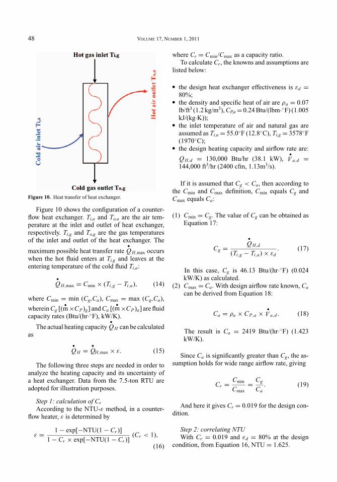
Figure 10. Heat transfer of heat exchanger.

Figure 10 shows the configuration of a counter-flow heat exchanger. Ti,a and To,a are the air tem-perature at the inlet and outlet of heat exchanger,respectively. Ti,g and To,g are the gas temperaturesof the inlet and outlet of the heat exchanger. The

maximum possible heat transfer rate•Q H,max occurs

when the hot fluid enters at Ti,g and leaves at theentering temperature of the cold fluid Ti,a:

•Q H,max = Cmin × (Ti,g − Ti,a), (14)

where Cmin = min (Cg,Ca), Cmax = max (Cg,Ca),

wherein Cg [(•m×CP )g] and Ca [(

•m×CP )a] are fluid

capacity rates (Btu/(hr·◦F), kW/K).

The actual heating capacity•Q H can be calculated

as

•Q H =

•QH,max × ε. (15)

The following three steps are needed in order toanalyze the heating capacity and its uncertainty ofa heat exchanger. Data from the 7.5-ton RTU areadopted for illustration purposes.

Step 1: calculation of Cr

According to the NTU-ε method, in a counter-flow heater, ε is determined by

ε = 1− exp[−NTU(1− Cr )]

1− Cr × exp[−NTU(1− Cr )](Cr < 1),

(16)

where Cr = Cmin/Cmax as a capacity ratio.To calculate Cr, the knowns and assumptions are

listed below:

� the design heat exchanger effectiveness is εd =80%;

� the density and specific heat of air are ρa = 0.07lb/ft3 (1.2 kg/m3), CP,a= 0.24 Btu/(lbm·◦F) (1.005kJ/(kg·K));

� the inlet temperature of air and natural gas areassumed as Ti,a = 55.0◦F (12.8◦C), Ti,g = 3578◦F(1970◦C);

� the design heating capacity and airflow rate are:

Q H,d = 130,000 Btu/hr (38.1 kW),•

V a,d =144,000 ft3/hr (2400 cfm, 1.13m3/s).

If it is assumed that Cg < Ca, then according tothe Cmin and Cmax definition, Cmin equals Cg andCmax equals Ca:

(1) Cmin = Cg. The value of Cg can be obtained asEquation 17:

Cg =•Q H,d

(Ti,g − Ti,a)× εd. (17)

In this case, Cg is 46.13 Btu/(hr·◦F) (0.024kW/K) as calculated.

(2) Cmax = Ca. With design airflow rate known, Ca

can be derived from Equation 18:

Ca = ρa × CP,a ו

V a,d . (18)

The result is Ca = 2419 Btu/(hr·◦F) (1.423kW/K).

Since Ca is significantly greater than Cg, the as-sumption holds for wide range airflow rate, giving

Cr = Cmin

Cmax= Cg

Ca. (19)

And here it gives Cr = 0.019 for the design con-dition.

Step 2: correlating NTUWith Cr = 0.019 and εd = 80% at the design

condition, from Equation 16, NTU = 1.625.

HVAC&R RESEARCH 49

Step 3: uncertainty analysis of•Q H

Combining Equations 15–19, for different oper-

ations,•Q H can be expressed as Equation 20:

•Q H =

•Q H,d

εd× ε =

•Q H,d

εd

×1− exp

[− NTU(1− Cg

Ca

)]1− Cg

Ca× exp

[− NTU(1− Cg

Ca

)] ,

Where NTU is an intermediate variable derivedfrom the variables of air side flow rate

•V a and gas-

heated side flow rate•

V g , as shown in Table 7.Therefore, fundamentally, uncertainty of heating

capacity calculation is conducted with the indepen-

dent variables of Va and Vg . The root sum square isused as Equation 21:

δ•Q H =

[(∂•Q H

∂•

V a

δ•

V a

)2

+(

∂•Q H

∂•

V g

δ•

V g

)2]1/2

,

(21)

where δ•

V a and δ•

V g are uncertainties.

δ•

V ais ±10%, which covers most conditions in

the real operations (e.g., fouling). δ•

V g has a lowvalue as ±1% because the natural gas regulatorholds a high accuracy of pressure control. Conse-quently, it is found that uncertainty of heating ca-pacity is only about ±2%. Heating capacity is verystable and can be treated as a constant by just refer-ring to the manufacturers’ design values.

50 VOLUME 17, NUMBER 1, 2011

Table 7. Calculation of NTU and uncertainty analysis of heating capacity.

Equations (ASHRAE 2009)

NTU UA, Cmin

ha ← Nua ← Rea ← Va ← V̇a ;hg ← Nug ← Reg ← Vg ← V̇g

NTU = UA/Cmin

Equation 22

⎧⎪⎪⎨⎪⎪⎩

1U A = 1

ha Aa+ li(Da/Dg)

2πkL + 1hg Ag

Equation 23

Cmin = Minimum (Ca, Cg)

⎧⎪⎪⎪⎪⎪⎪⎪⎪⎪⎪⎪⎪⎪⎪⎪⎪⎪⎪⎪⎪⎪⎪⎪⎪⎨⎪⎪⎪⎪⎪⎪⎪⎪⎪⎪⎪⎪⎪⎪⎪⎪⎪⎪⎪⎪⎪⎪⎪⎪⎩

ha = ka

DaNua Equation 24

Nua = 0.3+ 0.62Re1/2a Pr1/3

a

[1+0.4/ Pra )2/3]1/4 [1+ ( Rea

282,000 )1/2

(10, 000 < Rea < 40, 000) Equation 25

Rea = Va Da/va Equation 26

Va =•

Va /Aa Equation 27

hg = kg

DgNug Equation 28

Nug = 0.023Re4/5g Pr0.4

g (Reg > 10, 000)Equation 29

Reg = ρVg Dg/µg Equation 30

Vg = V̇g/Ag Equation 31

Symbols

A = area (ft2 (m2)) Pr = Prandtl numberC = heat air capacity rate ((Btu/(hr·◦F), kW/K)) Re = duct Reynolds numberD = duct diameter (in. (m)) U = heat transfer coefficient ((Btu/(hr·◦F·ft2),

kW/(m2·K)))h = heat transfer coefficient (Btu/h·ft2·◦F(kW/(m2·K))) v = kinematic viscosity (ft2/s(m2/s))k = thermal conductivity (Btu/h·ft·◦F (kW/(m·K))) V = linear velocity (ft/s(m/s))

L = duct length (ft (m))•

V = flow rate (ft3/s (m3/s))NTU = number of transfer units ρ = density (lbm/ft3(kg/m3))Nu = Nusselt number µ = absolute viscosity (lbm/ft·s ((N·s)/m2))

Uncertainty analysis of heating capacity

Independent variables Input Uncertainty

Flow rate of air side,•

V a , ft3/hr (m3/s) 144,000 (1.13) ±10%

Flow rate of gas heated air side,•

V g , ft3/hr (m3/s) 16,020 (0.13) ±1%

Dependent variable Output Uncertainty

Heating capacity,•Q H (Btu/hr (kW)) 130,000 (38.1) ±2%