1

Sensored Field Oriented Control of 3-Phase Permanent Magnet Synchronous Motors using LAUNCHXL- F28377S and BOOSTXL-DRV830x

Author: Ramesh T Ramamoorthy

Texas Instruments, Inc. C2000 Systems and Applications

2

Contents

Introduction ................................................................................................................................................ 3

PMSM Motors ............................................................................................................................................ 3

Field Oriented Control ............................................................................................................................... 5

Benefits of 32-bit C2000 Controllers for Digital Motor Control ............................................................... .11

TI Motor Control Literature and DMC Library .......................................................................................... 12

System Overview ..................................................................................................................................... 13

Hardware Configuration ........................................................................................................................... 15

Software Setup Instructions to Run HVPMSM_Sensored Project .......................................................... 21

Incremental System Build ........................................................................................................................ 30

Abstract This application note presents a solution to control a permanent magnet synchronous motor (PMSM) using the TMS320F2837x microcontrollers. TMS320F2837x devices are part of the family of C2000 microcontrollers which enable cost-effective design of intelligent controllers for three phase motors by reducing the system components and increase efficiency. With these devices it is possible to realize far more precise digital vector control algorithms like the Field Orientated Control (FOC). This algorithm’s implementation is discussed in this document. The FOC algorithm maintains efficiency in a wide range of speeds and takes into consideration torque changes with transient phases by processing a dynamic model of the motor. This application note covers the following:

A theoretical background on field oriented motor control principle.

Incremental build levels based on modular software blocks

Experimental results

3

Introduction A brushless Permanent Magnet Synchronous motor (PMSM) has a wound stator, a permanent magnet rotor assembly and internal or external devices to sense rotor position. The sensing devices provide position feedback for adjusting frequency and amplitude of stator voltage reference properly to maintain rotation of the magnet assembly. The combination of an inner permanent magnet rotor and outer windings offers the advantages of low rotor inertia, efficient heat dissipation, and reduction of the motor size. Moreover, the elimination of brushes reduces noise, EMI generation and suppresses the need of brushes maintenance. This document presents a solution to control a permanent magnet synchronous motor using the TMS320F28377S launch pad and integrated motor driver DRV830x BoosterPack. It enables cost-effective design of intelligent controllers for brushless motors which can fulfill enhanced operations, consisting of fewer system components, lower system cost and increased performances. The control method presented relies on the field orientated control (FOC). This algorithm maintains efficiency in a wide range of speeds and takes into consideration torque changes with transient phases by controlling the flux directly from rotor coordinates. This application report presents the implementation of a control for sinusoidal PMSM motor. The sinusoidal voltage waveform applied to this motor is created by using the Space Vector modulation technique. Minimum amount of torque ripple appears when driving this sinusoidal BEMF motor with sinusoidal currents.

Permanent Magnet Motors There are primarily two types of three-phase permanent magnet synchronous motors. One uses rotor windings fed from the stator and the other uses permanent magnets. A motor fitted with rotor windings, requires brushes to obtain its current supply and generate rotor flux. The contacts are made of rings and have any commutator segments. The drawbacks of this type of structure are maintenance needs and lower reliability. Replacing the common rotor field windings and pole structure with permanent magnets puts the motor into the category of brushless motors. It is possible to build brushless permanent magnet motors with any even number of magnet poles. The use of magnets enables an efficient use of the radial space and replaces the rotor windings, therefore suppressing the rotor copper losses. Advanced magnet materials permit a considerable reduction in motor dimensions while maintaining a very high power density.

Figure 1 A three-phase synchronous motor with one permanent magnet

pair pole rotor

4

Synchronous Motor Operation

Synchronous motor construction: Permanent magnets are rigidly fixed to the rotating axis to create a constant rotor flux. The stator windings when energized with three phase voltages create a rotating electromagnetic field. To control the rotating magnetic field, it is necessary to control the stator currents.

The actual structure of the rotor varies depending on the power range and rated speed of the machine. Permanent magnets are suitable for synchronous machines ranging up-to a few Kilowatts. For higher power ratings the rotor usually consists of windings in which a DC current circulates. The mechanical structure of the rotor is designed for number of poles desired, and the desired flux gradients.

The interaction between the stator and rotor fluxes produces a torque. Since the stator is firmly mounted to the frame, and the rotor is free to rotate, the rotor will rotate, producing a useful mechanical output.

The angle between the rotor magnetic field and stator field must be carefully controlled to produce maximum torque and achieve high electromechanical conversion efficiency. For this purpose a fine tuning is needed after closing the speed loop in order to draw minimum amount of current under the same speed and torque conditions.

The stator field must rotate at the same frequency as the rotor field; otherwise the rotor will experience rapidly alternating positive and negative torque. This will result in less than optimal torque production, and excessive mechanical vibration, noise, and mechanical stresses on the machine parts. In addition, if the rotor inertia prevents the rotor from being able to respond to these oscillations, the rotor will stop rotating at the synchronous frequency, and respond to the average torque as seen by the stationary rotor: Zero. This means that the machine experiences a phenomenon known as ‘pull-out’. This is also the reason why the synchronous machine is not self starting.

The angle between the rotor field and the stator field must be equal to 90º to produce maximum torque. This synchronization requires knowing the rotor position in order to generate the right stator field.

The stator magnetic field can be made to have any direction and magnitude by combining the contribution of different stator phase currents to produce the resulting stator flux.

Figure 2 The interaction between the rotating stator flux, and the rotor flux produces a torque which will cause the motor to rotate.

5

Field Oriented Control

Introduction In order to achieve better dynamic performance, a more complex control scheme needs to be applied, to control the PM motor. With the mathematical processing power offered by the microcontrollers, we can implement advanced control strategies, which use mathematical transformations to control AC machines like DC machines, providing independent control of flux and torque producing currents. Such de-coupled torque and magnetization control is commonly called Field Oriented Control (FOC).

The main philosophy behind the FOC

In order to understand the spirit of the Field Oriented Control technique, let us start with an overview of the separately excited direct current (DC) Motor. Torque is defined as the cross product of armature current and stator flux. Electrical study of the DC motor shows that the armature current and the stator flux can be independently tuned. The strength of the field excitation (i.e. the magnitude of the field excitation current) sets the value of the stator flux. If the flux is held constant, then the current through the rotor windings determines how much torque is produced. The commutator on the rotor plays an interesting part in the torque production. The commutator is in contact with the brushes, and the mechanical construction is designed to switch into the circuit the windings that are mechanically aligned to produce the maximum torque. This arrangement then means that the torque production of the machine is fairly near optimal all the time. The key point here is that the windings are managed to keep the flux produced by the rotor windings orthogonal to the stator field/current.

AC machines do not have the same key features as the DC motor. The flux and torque producing current are not necessarily orthogonal. In PM synchronous machines, the rotor excitation is given by the permanent magnets mounted onto the shaft and stator carries the torque producing current. In induction machines, the stator carries both flux producing and torque producing currents and its only source of power is the stator phase voltage. The flux and torque producing components of currents are strongly coupled unlike in a DC machine. The goal of the FOC (also called vector control) on synchronous and asynchronous machine is to be able to control those like a separately excited DC machine wherein the flux producing and torque producing currents are separately controlled. In other words, the control technique goal is, in a sense, to imitate the control of a DC motor. FOC control will allow us to decouple the flux and torque producing currents enabling them to be controlled independently. To decouple the torque and flux producing currents, it is necessary to engage several mathematical transforms, and this is where the microcontrollers add the most value. The processing capability provided by the microcontrollers enables these mathematical transformations to be carried out very quickly. This in turn implies that the entire algorithm controlling the motor can be executed at a fast rate, enabling higher dynamic performance. In addition to the decoupling, a dynamic model of the motor is now used for the computation of many quantities such as rotor flux angle and rotor speed. This means that their effect is accounted for, and the overall quality of control is better.

Fig 3 Separately excitated DC motor model, flux and torque are independently controlled and the current through the rotor windings determines how much torque is produced.

)(..

..

e

em

IfKE

IKT

Inductor (field excitation)

Armature Circuit

6

Torque can be defined in multiple ways, as the cross product of stator current and rotor flux, or, as the cross product of stator flux and rotor flux as given below

rotorstatorem BBT

, or, rotorstatorem BIT

This expression shows that the torque is at a maximum for any given stator and rotor magnetic fields when they are orthogonal. If we are able to ensure this condition all the time, if we are able to orient the flux correctly, we reduce the torque ripple and we ensure a better dynamic response. However, the constraint is to know the rotor position: this can be achieved with a position sensor such as incremental or absolute encoder/ resolver. For low-cost application where the rotor is not accessible, different rotor position observer strategies can be applied to get rid of position sensor. A 3 phase PM synchronous machine can be represented as a DC machine in synchronous DQ reference frame, where the D-axis is aligned along the rotor magnet flux and the Q axis is orthogonal to D axis. Any current flowing along D-axis, called direct component of current, can impact the strength of magnetic field and the current in Q axis, called quadrature current, will interact with the magnetic flux in D-axis to produce torque. In brief, for a PM motor, the goal is to maintain the d-axis current at zero and adjust the magnitude of current in Q-axis to generate the commanded torque. The direct component of the stator current can be kept negative in some cases for field weakening, which has the effect of reducing the rotor flux, and reducing the back-emf allowing for operation at higher speeds. Technical Background The Field Orientated Control effectively controls the stator current vector. This control is based on projections which transform a three phase, time variant system into a two co-ordinate (d and q co-ordinates) time invariant system. These projections lead to a structure similar to that of a DC machine control. Field orientated controlled machines need two constants as input references: the torque component (aligned with the q co-ordinate) and the flux component (aligned with d co-ordinate). As Field Orientated Control is simply based on projections the control structure handles instantaneous electrical quantities. This makes the control accurate in every working operation (steady state and transient) and independent of the limited bandwidth mathematical model. The FOC thus solves the classic scheme problems, in the following ways:

The ease of reaching constant reference (torque component and flux component of the stator current)

The ease of torque control because in the (d,q) reference frame the expression of the torque is:

SqR im

By maintaining the amplitude of the rotor flux ( R ) at a fixed value we have a linear relationship

between torque and torque component of stator current vector (iSq). We can then control the torque by controlling the torque component.

Space Vector Definition and Projection The three-phase voltages, currents and fluxes of AC-motors can be analyzed in terms of complex space vectors. With regard to the currents, the space vector can be defined as follows. Assuming that

ia, ib, ic are the instantaneous currents in the stator phases, then the complex stator current vector si is

defined by:

cbas iiii 2

7

where

3

2j

e and

3

4

2j

e , represent the spatial operators. The following diagram shows the stator

current complex space vector:

Figure 4 Stator current space vector and its component in (a,b,c)

where (a,b,c) are the three phase system axes. This current space vector depicts the three phase sinusoidal system. It still needs to be transformed into a two time invariant co-ordinate system. This transformation can be split into two steps:

(a,b,c) ),( (the Clarke transformation) which outputs a two co-ordinate time variant system

),( (d,q) (the Park transformation) which outputs a two co-ordinate time invariant system

The (a,b,c) ),( Projection (Clarke transformation)

The space vector can be reported in another reference frame with only two orthogonal axis called ),( .

Assuming that the axis a and the axis are in the same direction we have the following vector diagram:

Figure 5 Stator current space vector and its components in the stationary reference frame

The projection that modifies the three phase system into the ),( two dimension orthogonal system is

presented below.

bas

as

iii

ii

3

2

3

1

8

The two phase ),( currents still depends on time and speed.

The ),( (d,q) Projection (Park Transformation)

This is the most important transformation in the FOC. In fact, this projection modifies a two phase

orthogonal system ),( in the d,q rotating reference frame. If we consider the d axis aligned with the

rotor flux, the next diagram shows, for the current vector, the relationship from the two reference frame:

Figure 6 Stator current space vector and its component in ),( and in

d,q rotating reference frame

where θ is the rotor flux position. The flux and torque components of the current vector are determined by the following equations:

cossin

sincos

sssq

sssd

iii

iii

These components depend on the current vector ),( components and on the rotor flux position; if we

know the right rotor flux position then, by this projection, the d,q component becomes a constant. Two phase currents now turn into dc quantity (time-invariant). At this point the torque control becomes easier where constant isd (flux component) and isq (torque component) current components controlled independently.

9

The Basic Scheme for the FOC The following diagram summarizes the basic scheme of torque control with FOC:

Figure 7 Basic scheme of FOC for AC motor

Two motor phase currents are measured. These measurements feed the Clarke transformation module. The outputs of this projection are designated isα and isβ. These two components of the current along with rotor flux position are the inputs of the Park transformation, which transform them to currents (isd and isq) in d,q rotating reference frame. The isd and isq components are compared to the references isdref (the flux reference) and isqref (the torque reference). At this point, this control structure shows an interesting advantage: it can be used to control either synchronous or HVPM machines by simply changing the flux reference and obtaining rotor flux position. In synchronous permanent magnet motor, the rotor flux is fixed as determined by the magnets. Hence there is no need to create it. Hence, when controlling a PMSM, isdref should be set to zero. As ACIM motors need a rotor flux creation in order to operate, the flux reference must not be zero. This conveniently solves one of the major drawbacks of the “classic” control structures: the portability from asynchronous to synchronous drives. The torque command isqref can be connected to the output of the speed regulator. The outputs of the current regulators are Vsdref and Vsqref; they are applied to the inverse Park transformation. Using the position of rotor flux, this projection generates Vsαref and Vsβref which are the components of the stator vector

voltage in the ),( stationary orthogonal reference frame. These are the inputs of the Space Vector

PWM. The outputs of this block are the signals that drive the inverter. Note that both Park and inverse Park transformations need the rotor flux position. Obtaining this rotor flux position depends on the AC machine type (synchronous or asynchronous machine). Rotor flux position considerations are made in a following paragraph.

Rotor Flux Position

Knowledge of the rotor flux position is the core of the FOC. In fact if there is an error in this variable the rotor flux is not aligned with d-axis and isd and isq will represent incorrect flux and torque components of

the stator current. The following diagram shows the (a,b,c), ),( and (d,q) reference frames, and the

correct position of the rotor flux, the stator current and stator voltage space vector that rotates with d,q reference frame at synchronous speed.

10

Figure 8 Current, voltage and rotor flux space vectors in the d,q rotating reference frame and their

relationship with a,b,c and ),( stationary reference frame

The measure of the rotor flux position is different if we consider synchronous or asynchronous motors:

In the synchronous machine the rotor speed is equal to the rotor flux speed. Then θ (rotor flux position) is directly measured by position sensor or by integration of rotor speed.

In the asynchronous machine the rotor speed is not equal to the rotor flux speed (there is a slip speed), then it needs a particular method to calculate θ. The basic method is the use of the current model which needs two equations of the motor model in d,q reference frame.

Theoretically, the field oriented control for PMSM drive allows the motor torque be controlled independently like DC motor. In other words, the torque component of current and flux are decoupled from each other. The rotor position is required for variable transformation from stationary reference frame to synchronously rotating reference frame. Therefore, the key module of this system is the information of rotor position from QEP encoder. The overall block diagram of this project is depicted in Figure 9.

Figure 9 Overall block diagram of Sensored Field Oriented Control

11

Benefits of 32-bit C2000 Controllers for Digital Motor Control (DMC) C2000 family of devices posses the desired computation power to execute complex control algorithms along with the right mix of peripherals to interface with the various components of the DMC hardware like the ADC, ePWM, QEP, eCAP etc. These peripherals have all the necessary hooks for implementing systems which meet safety requirements, like the trip zones for PWMs and comparators. Along with this the C2000 ecosystem of software (libraries and application software) and hardware (application kits) help in reducing the time and effort needed to develop a Digital Motor Control solution. The DMC Library provides configurable blocks that can be reused to implement new control strategies. IQMath Library enables easy migration from floating point algorithms to fixed point thus accelerating the development cycle. Thus, with C2000 family of devices it is easy and quick to implement complex control algorithms (sensored and sensorless) for motor control. The use of C2000 devices and advanced control schemes provides the following system improvements

Favors system cost reduction by an efficient control in all speed range implying right dimensioning of power device circuits

Using advanced control algorithms, it is possible to reduce torque ripple, thus resulting in lower vibration and longer life time of the motor

Advanced control algorithms reduce harmonics generated by the inverter thus reducing filter cost.

Use of sensorless algorithms eliminates the need for speed or position sensor.

Decreases the number of look-up tables which reduces the amount of memory required

The Real-time generation of smooth near-optimal reference profiles and move trajectories, results in better-performance

Generation of high resolution PWM’s is possible with the use of ePWM peripheral for controlling the power switching inverters

Provides single chip control system

For advanced controls, C2000 controllers can also perform the following:

Enables control of multi-variable and complex systems using modern intelligent methods such as neural networks and fuzzy logic.

Performs adaptive control. C2000 controllers have the speed capabilities to concurrently monitor the system and control it. A dynamic control algorithm adapts itself in real time to variations in system behaviour.

Performs parameter identification for sensorless control algorithms, self-commissioning, online parameter estimation update.

Performs advanced torque ripple and acoustic noise reduction.

Provides diagnostic monitoring with spectrum analysis. By observing the frequency spectrum of mechanical vibrations, failure modes can be predicted in early stages.

12

Produces sharp-cut-off notch filters that eliminate narrow-band mechanical resonance. Notch filters remove energy that would otherwise excite resonant modes and possibly make the system unstable.

TI Literature and Digital Motor Control (DMC) Library The Digital Motor Control (DMC) library is composed of functions represented as blocks. These blocks are categorized as Transforms & Estimators (Clarke, Park, Sliding Mode Observer, Phase Voltage Calculation, and Resolver, Flux, and Speed Calculators and Estimators), Control (Signal Generation, PID, BEMF Commutation, Space Vector Generation), and Peripheral Drivers (PWM abstraction for multiple topologies and techniques, ADC drivers, and motor sensor interfaces). Each block is a modular software macro is separately documented with source code, use, and technical theory. Check the folders below for the source codes and explanations of macro blocks: C:\TI\controlSUITE\libs\app_libs\motor_control\math_blocks\v4.0 C:\TI\controlSUITE\libs\app_libs\motor_control\drivers\f2803x_v2.0 These modules allow users to quickly build, or customize, their own systems. The Library supports the three motor types: ACI, BLDC, PMSM, and comprises both peripheral dependent (software drivers) and target dependent modules. The DMC Library components have been used by TI to provide system examples. At initialization all DMC Library variables are defined and inter-connected. At run-time the macro functions are called in order. Control system is built using an incremental build approach, which allows some sections of the code to be built at a time, so that the developer can verify each section of their application one step at a time. This is critical in real-time control applications where so many different variables can affect the system and many different motor parameters need to be tuned. Note: TI DMC modules are written in form of macros for optimization purposes (refer to application note SPRAAK2 for more details at TI website). The macros are defined in the header files. The user can open the respective header file and change the macro definition, if needed. In the macro definitions, there should be a backslash ”\” at the end of each line as shown below which means that the code continue in the next line. Any character including invisible ones like “space” after the backslash will cause compilation error. Therefore, make sure that the backslash is the last character in the line. In terms of code development, the macros are almost identical to C function, and the user can easily convert the macro definition to a C functions.

#define PARK_MACRO(v) \

\

v.Ds = _IQmpy(v.Alpha,v.Cosine) + _IQmpy(v.Beta,v.Sine); \

v.Qs = _IQmpy(v.Beta,v.Cosine) - _IQmpy(v.Alpha,v.Sine);

A typical DMC macro definition

13

System Overview This document describes the “C” real-time control framework used to demonstrate the sensored field oriented control of HVPM motors. The “C” framework is designed to run on C2000 based controllers on Code Composer Studio. The framework uses the following modules

1:

Macro Names Explanation

CLARKE Clarke Transformation

PARK / IPARK Park and Inverse Park Transformation

PI PI Regulators

PID PID Regulator

PI_POS PI Regulator for position loop

RC Ramp Controller (slew rate limiter)

RG Ramp / Sawtooth Generator

QEP QEP Drive

SPEED_FR Speed Measurement (based on sensor signal frequency)

SVGEN Space Vector PWM with Quadrature Control (includes IClarke Trans.)

PWM PWM Drives 1 Please refer to pdf documents in motor control folder explaining the details and theoretical background of each macro

The overall system implementing sensored Field Oriented Control (FOC) of Permanent Magnet Synchronous Motor (PMSM) is depicted in Figure 10. The PM motor is driven using a DRV830x BoosterPack (BOOSTXL-DRV8301/5) that has an integrated motor driver device DRV8301/5. Launch pad LAUNCHXL-F28377S, that has a TMS320F28377S CPU, is used to generate three sets of complementary pulse width modulation (PWM) signals for the inverter. Two/three phase currents of PM motor are measured from the inverter using shunt resistors connected to the bottom of inverter half bridges, which are amplified by shunt current amplifiers of the DRV830x driver. The amplified shunt voltage is then measured using ADCs. The DC-bus voltage of the inverter, as well as the motor phase voltages, is measured using ADC.

2B

2A

V-dcBus

3B

3A

3 phs Inverter

110/220V

Va

Vb

Vc

IPM

Vin Vout 12V / 5V

3phs Motor

1A

1B

Encoder

Feedback

C2000 Piccolo

Ia Ib Ic

Figure 10 A 3-ph PM motor drive implementation

14

The software flow is described in the Figure 11 below.

c_int0

Initialize h/w

modules

Initialize s/w

modules

Enable end of

conversion ISR

Initialize other

system and module

parameters

Background

LoopINT 1

SOC

EOC ISR

Save contexts and

clear interrupt flag

Execute ADC

conversion

Execute the park

and clarke trans.

Execute the PID

modules

Execute the ipark

and svgen modules

Execute the

Position Encoder

Suite

Execute the PWM

drive

Restore context Return

Figure 11 Software flow sequence

15

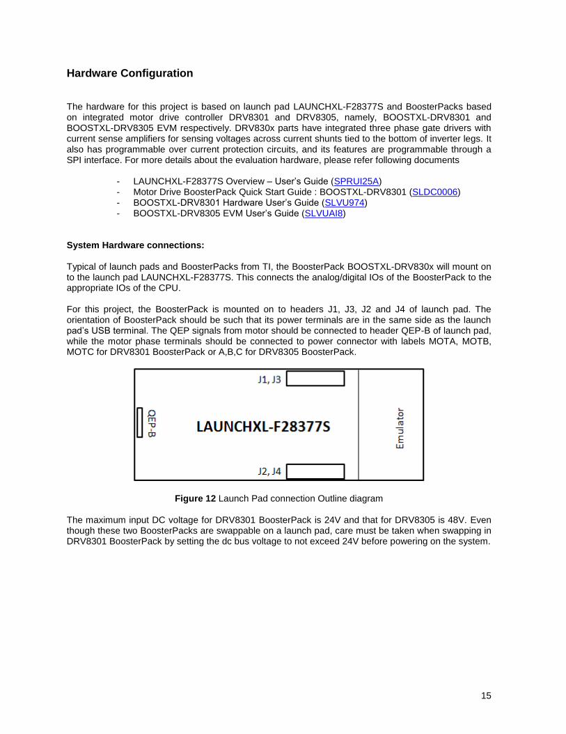
Hardware Configuration

The hardware for this project is based on launch pad LAUNCHXL-F28377S and BoosterPacks based on integrated motor drive controller DRV8301 and DRV8305, namely, BOOSTXL-DRV8301 and BOOSTXL-DRV8305 EVM respectively. DRV830x parts have integrated three phase gate drivers with current sense amplifiers for sensing voltages across current shunts tied to the bottom of inverter legs. It also has programmable over current protection circuits, and its features are programmable through a SPI interface. For more details about the evaluation hardware, please refer following documents

- LAUNCHXL-F28377S Overview – User’s Guide (SPRUI25A) - Motor Drive BoosterPack Quick Start Guide : BOOSTXL-DRV8301 (SLDC0006) - BOOSTXL-DRV8301 Hardware User’s Guide (SLVU974) - BOOSTXL-DRV8305 EVM User’s Guide (SLVUAI8)

System Hardware connections: Typical of launch pads and BoosterPacks from TI, the BoosterPack BOOSTXL-DRV830x will mount on to the launch pad LAUNCHXL-F28377S. This connects the analog/digital IOs of the BoosterPack to the appropriate IOs of the CPU. For this project, the BoosterPack is mounted on to headers J1, J3, J2 and J4 of launch pad. The orientation of BoosterPack should be such that its power terminals are in the same side as the launch pad’s USB terminal. The QEP signals from motor should be connected to header QEP-B of launch pad, while the motor phase terminals should be connected to power connector with labels MOTA, MOTB, MOTC for DRV8301 BoosterPack or A,B,C for DRV8305 BoosterPack.

Figure 12 Launch Pad connection Outline diagram The maximum input DC voltage for DRV8301 BoosterPack is 24V and that for DRV8305 is 48V. Even though these two BoosterPacks are swappable on a launch pad, care must be taken when swapping in DRV8301 BoosterPack by setting the dc bus voltage to not exceed 24V before powering on the system.

16

Powering the launch pad: For immediate reference, layout of LAUNCHXL-F28377S and the pinouts of LAUNCHXL-F28377S, BOOSTXL-DRV8301 and BOOSTXL-DRV8305 are given below

Figure 13 Layout of LAUNCHXL-F28377S For early code development without the BoosterPack, it is ok to retain the jumpers JP1 and JP2 of the launch pad. This feeds 3.3V power from the emulator section to the CPU. Alternately, the CPU can be powered from an external source through the header pins of header J1, J3 or J5 and J7, in which case remove jumpers JP1 and JP2. Make sure to remove these jumpers or external power supply before mounting the DRV BoosterPack because the BoosterPack is designed to power the launch pad when mounted. Jumpers JP4 and JP5 on the launch pad are meant to provide power supply to any booster pack mounted on headers J5, J6, J7 and J8. However, if the booster pack generates its own power supply, then do not populate JP4 and JP5. If there is no booster pack on J5-J8, then JP4 and JP5 are don’t care.

CAUTION:

If these jumpers are present when the BoosterPack is powered, then it can

1. Potentially damage the development computer as it will tie the computer’s USB to external power supply GND.

2. Create circulating current between the 3.3V power supplies generated by the DRV BoosterPack and the emulator powered by USB.

17

LAUNCHXL F28377S Pin out and GPIO pin MUX options – Header J1, J3

Mux value J1 pin J3 pin Mux value

3 2 1 0 0 1 2 3

+3.3V 1 21 +5V

EM1D13 GPIO71 2 22 GND

EM1DQM2 EM1A17 GPIO90 3 23 ADCIN14

EM1DQM1 EM1A16 GPIO89 4 24 ADCINB1

EM1A3 GPIO41 5 25 ADCINB4

---- 6 26 ADCINB2

EM2D8 EM1D24 MCLKRB GPIO60 7 27 ADCINA0

EM2D7 EM1D23 MFSRB GPIO61 8 28 ADCINB0

GPIO43 9 29 ADCINA4

10 20 ----

Pin out and GPIO pin MUX options – Header J4, J2

Mux value J4 pin

J2 pin

Mux value

3 2 1 0 0 1 2 3

MDXB CANTXB EPWM7A GPIO12 40 20 GND

MDRB CANRXB EPWM7B GPIO13 39 19 GPIO4 EPWM3A

MCLKXB SCITXDB EPWM8A GPIO14 38 18 GPIO62 SCIRXDC EM1D2 EM2D6

MFSXB SCIRXDB EPWM8B GPIO15 37 17 ----

OUTPUTXBAR7 CANTXB SPISIMOA GPIO16 36 16 RESET#

OUTPUTXBAR6 CANRXB SPISOMIA GPIO17 35 15 GPIO58 MCLKRA EM1D26 EM2D10

CANTXB MDXA EQEP1A GPIO20 34 14 GPIO59 MFSRA EM1D25 EM2D9

CANRXB MDRA EQEP1B GPIO21 33 13 GPIO72 EM1D12

DAC1 32 12 GPIO73 EM1D11 XCLKOUT

DAC2 31 11 GPIO78 EM1D6

18

Pin out and GPIO pin MUX options – Header J5, J7

Mux value J5 pin J7 pin Mux value

3 2 1 0 0 1 2 3

+3.3V 41 61 +5V

---- 42 62 GND

EM1RAS EM1A14 GPIO87 43 63 ADCIN15

EM1CAS EM1A13 GPIO86 44 64 ADCINA2

---- 45 65 ADCINA5

---- 46 66 ADCINB5

EM1D19 GPIO65 47 67 ADCINA3

48 68 ADCINB3

EM1D15 GPIO69 49 69 ADCINA4

EM1D18 GPIO66 50 70 ----

Pin out and GPIO pin MUX options – Header J8, J6

Mux value J8 pin

J6 pin

Mux value

3 2 1 0 0 1 2 3

EPWM1A GPIO2 80 60 GND

EPWM1B GPIO3 79 59 GPIO91 EM1A18 EEM1DQM3

ADCSOCB0 CANRXB EPWM6A GPIO10 78 58 ----

OUTPUTXBAR7 SCIRXDB EPWM6B GPIO11 77 57 ----

CANRXA SCITXDB SPICLKA GPIO18 76 56 RESET#

CANTXA SCIRXDB SPISTEA GPIO19 75 55 GPIO63 SCITXDC EM1D21 EM2D5

---- 74 54 GPIO64 EM1D20 EM2D4

---- 73 53 GPIO99 EM2A1

DAC3 72 52 GPIO92 EM1D19 EM1BA1

DAC4 71 51 ----

19

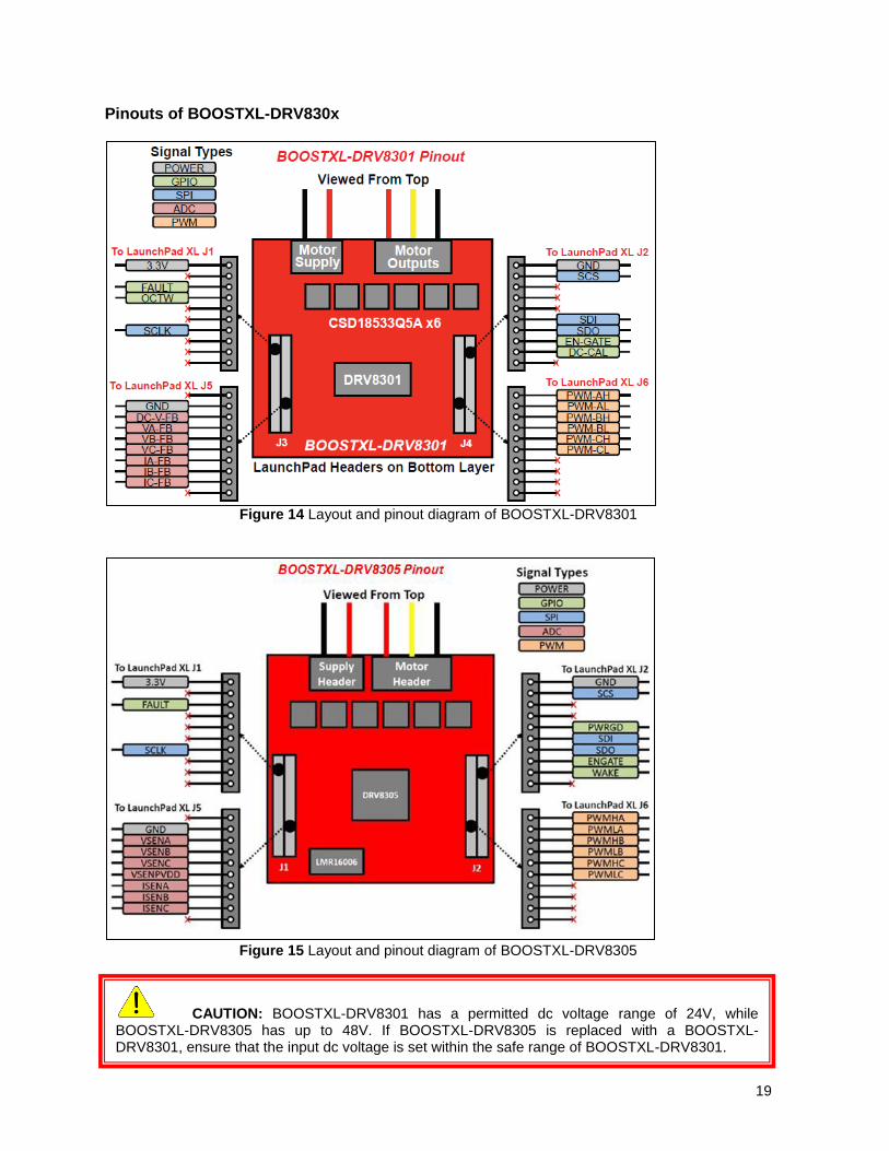
Pinouts of BOOSTXL-DRV830x

Figure 14 Layout and pinout diagram of BOOSTXL-DRV8301

Figure 15 Layout and pinout diagram of BOOSTXL-DRV8305

CAUTION: BOOSTXL-DRV8301 has a permitted dc voltage range of 24V, while

BOOSTXL-DRV8305 has up to 48V. If BOOSTXL-DRV8305 is replaced with a BOOSTXL-DRV8301, ensure that the input dc voltage is set within the safe range of BOOSTXL-DRV8301.

20

NOTE :

When executing standalone FLASH Projects with BOOSTXL-DRV8301, there is an issue with starting

the CPU out of RESET. The DRV301 kit’s EN_GATE signal is tied to GPIO72 of the CPU in launch

pad. GPIO72 is one of the BOOT mode pins that determine how the CPU will boot coming out of

RESET. Since this signal is pulled LOW with a pull down resistor (R6) in the DRV8301 kit, the CPU will

try to boot in an unsupported mode and fail to run. Therefore, it is recommended to safely remove the

pull down resistor for testing in standalone FLASH projects. This does not affect the functionality or

safety of the BOOSTXL-DRV8301 kit.

21

Software Setup for LaunchXS Projects

Installing Code Composer and controlSUITE

1. If not already installed, please install Code Composer v6.x or later from http://www.ti.com/tool/CCSTUDIO

2. Go to http://www.ti.com/controlsuite and run the controlSUITE installer. Allow the installer to

download and update any automatically checked software for C2000.

Setup Code Composer Studio for Project Evaluation

3. Open “Code Composer Studio”. Note that this document assumes version 6 or later.

4. Once Code Composer Studio opens, the workspace launcher may appear that would ask to select a workspace location,: (please note workspace is a location on the hard drive where all the user settings for the IDE i.e. which projects are open, what configuration is selected etc. are saved, this can be anywhere on the disk, the location mentioned below is just for reference. Also note that if this is not your first-time running Code Composer the dialog below may not appear)

Click the “Browse…” button

Create the path below by making new folders as necessary.

“C:\c2000 projects\CCSv6_workspaces\XL377s_DRV_workspace”

Uncheck the box that says “Use this as the default and do not ask again”.

Click “OK”

Figure 16 Workspace Launcher

5. This will open a ‘Getting Started’ tab with links to various tasks from creating a new project, importing an existing project to watching a Tutorial on CCS.

22

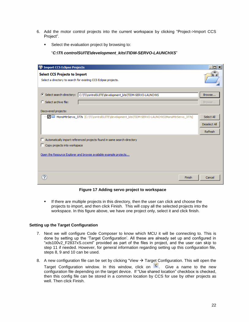
6. Add the motor control projects into the current workspace by clicking “Project->Import CCS Project”.

Select the evaluation project by browsing to:

“C:\TI\ controlSUITE\development_kits\TIDM-SERVO-LAUNCHXS”

Figure 17 Adding servo project to workspace

If there are multiple projects in this directory, then the user can click and choose the projects to import, and then click Finish. This will copy all the selected projects into the workspace. In this figure above, we have one project only, select it and click finish.

Setting up the Target Configuration

7. Next we will configure Code Composer to know which MCU it will be connecting to. This is done by setting up the ‘Target Configuration’. All these are already set up and configured in “xds100v2_F2837xS.ccxml” provided as part of the files in project, and the user can skip to step 11 if needed. However, for general information regarding setting up this configuration file, steps 8, 9 and 10 can be used.

8. A new configuration file can be set by clicking “View Target Configuration. This will open the

Target Configuration window. In this window, click on . Give a name to the new configuration file depending on the target device. If “Use shared location” checkbox is checked, then this config file can be stored in a common location by CCS for use by other projects as well. Then click Finish.

23

9. This should open up a new tab as shown in Figure 18. Select and enter the options as shown:

Connection – Texas Instruments XDS100v2 USB Emulator (or)

Texas Instruments XDS100v2 USB Debug Probe

Device – the C2000 MCU on the control card, TMS320F28377S, for example

Click Save and close

Figure 18 Configuring a new target

10. To use this configuration file, click “View->Target Configurations”. In the “User Defined” section,

find the file that was created in step 8, 9 and 10. Right-click on this file and select “Set as Default”.

11. To use the configuration file supplied with the project, click “View->Target Configurations, then expand “ProjectsMonoMtrServo_377s” and right-click on the file “xds100v2_F2837xS.ccxml” and “Set as Default”. This tab also allows you to reuse existing target configurations and link them to specific projects.

24

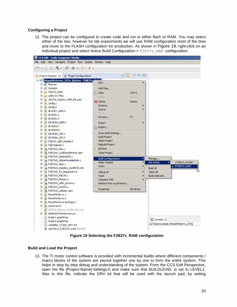
Configuring a Project

12. The project can be configured to create code and run in either flash or RAM. You may select either of the two, however for lab experiments we will use RAM configuration most of the time

and move to the FLASH configuration for production. As shown in Figure 19, right-click on an

individual project and select Active Build Configuration-> F2837x_RAM configuration.

Figure 19 Selecting the F2837x_RAM configuration

Build and Load the Project

13. The TI motor control software is provided with incremental builds where different components / macro blocks of the system are pieced together one by one to form the entire system. This helps in step by step debug and understanding of the system. From the CCS Edit Perspective, open the file [Project-Name]-Settings.h and make sure that BUILDLEVEL is set to LEVEL1. Also in this file, indicate the DRV kit that will be used with the launch pad, by setting

25

MOTOR1_DRV to DRV8301 or DRV8305 and save this file. After testing build 1, the variable BUILDLEVEL will need to be redefined to move on to build 2, and so on until all builds are complete.

14. Open the [Project-Name].c file and go to the function BuildLevel1(). Locate the following piece of code in incremental build 1 and confirm that the Datalog buffers are pointing to the right variables. These Datalog buffers are large arrays that contain value-triggered data that can then be displayed to a graph. Note that in other incremental builds different variables may be put into this buffer to be graphed. Following is an example where the datalog are pointed to the space vector generator module.

DlogCh1=rg1.Out; DlogCh2=svgen1.Ta; DlogCh3=svgen1.Tb; DlogCh4=svgen1.Tc;

15. Now Right Click on the Project Name and click on “Rebuild Project” and watch the Console window. Any errors in the project will be displayed, which needs to be fixed. There may be some warning messages about certain functions or variables not being used. Such warning messages may be ignored, as they may be used in another build level.

Connecting the hardware to computer

16. Remove jumpers JP1 and JP2 from launch pad LAUNCHXL-F28377S, and mount booster pack BOOSTXL-DRV830x on launch pad headers J1-J4. DO NOT connect motor right now. Power the booster pack with appropriate input dc voltage, 24V for DRV8301 and 48V for DRV8305. This will glow various LEDs on both booster pack and launch pad. Now connect the launch pad to computer through an USB cable. This will light some LEDs on the emulator section of launch pad, indicating that the emulator is on.

17. Continuing from step 15, on successful completion of the build, click the “Debug” button, located in the top-left side of the screen.

18. The IDE will now connect to the target, load the output file into the device and change to the Debug perspective.

19. Click “Tools->Debugger Options->Program / Memory Load Options”. You can enable the debugger to reset the processor each time it reloads program by checking “Reset the target on program load or restart” and click “Remember My Settings” to make this setting permanent.

20. Now click on the “Enable silicon real-time mode” button which also auto selects “Enable

polite real-time mode” button . This will allow the user to edit and view variables in real-time. Do not reset the CPU without disabling these real time options!

21. A message box may appear. If so, select YES to enable debug events. This will set bit 1 (DGBM bit) of status register 1 (ST1) to a “0”. The DGBM is the debug enable mask bit. When the DGBM bit is set to “0”, memory and register values can be passed to the host processor for updating the debugger windows.

26

Setup Expressions Window & Graphs

Click: View Expressions on the menu bar to open an Expressions window to view the

variables being used in the project. Add variables to the expressions window as shown below. It uses the number format associated with variables during declaration. You can select a desired number format for the variable by right clicking on it and choosing. Figure below shows a typical expressions window.

Figure 20 Configuring the Expressions Window

Alternately, a group of variables can be imported into the Expressions window, by right clicking within Expressions Window and clicking Import, and browse to the .txt file containing these variables. Here, browse to the root directory of the project and pick ‘variables_377sXL_DRV.txt’ and click OK to import the variables shown in Figure 20.

The structure variable ‘motor1’ has references to all peripherals and variables that are related to controlling the motor. By expanding this variable, the user can see them all and edit as needed.

Figure 21 Variables within structure ‘motor1’

22. Click on the Continuous Refresh button in the expressions window. This enables the window to run with real-time mode. By clicking the down arrow in this expressions window, you may select “Customize Continuous Refresh Interval” and edit the refresh rate of the expressions window. Note that choosing too fast an interval may affect performance.

27

23. The datalog buffers point to different system variables depending on the build level. They provide a means to visually inspect the variables and judge system performance. Open and setup time graph windows to plot the data log buffers as shown below. Alternatively, the user can import graph configurations files in the project folder by clicking: Tools -> Graph -> DualTime… and select import and browse to the following location

C:\TI\controlSUITE\development_kits\TIDM-SERVO-LAUNCHXS\MonoMtrServo_377s

and select Graph1.graphProp, the Graph Properties window should now look like the Figure 22. Hit OK, this should add the Graphs to your debug perspective. Click on Continuous Refresh button on the top left corner of the graph tab.

Note: If a second graph window is used, you could import Graph2.prop, the start Addresses for this should be DBUFF_4CH3 and DBUFF_4CH4.

Note: The default dlog.prescaler is set to 5 which will allow the dlog function to only log one out of every five samples.

Note: The default dlog.trig_value should be set to the right value to generate trigger for the plot as in oscilloscopes.

Figure 22 Graph window settings

28

Run the Code

24. Run the code by pressing Run Button in the Debug Tab.

25. In the Expressions window, set the variable ‘EnableFlag’ to 1.

26. The project should now run, and the values in the graphs and expressions window should continuously update. Below are some screen captures of typical CCS perspectives while using this project. You may want to resize the windows according to your preference. At this time, details of variables and graph are not discussed as they will be discussed in later sections

27. Once complete, turn off Real Time mode, then reset the processor (Run->Reset->CPU

Reset) and then terminate the debug session by clicking (Run->Terminate). This will halt the program and disconnect Code Composer from the MCU.

Figure 23 CCS IDE showing Edit Perspective

29

Figure 24 CCS IDE showing Debug Perspective

Next Steps

28. It is not necessary to terminate the debug session each time the user changes or runs the code again. Instead the following procedure can be followed. After rebuilding the project, (Run-

>Reset->CPU Reset) , (Run->Restart ) , and enable realtime options. Once complete, disable real time options, and reset CPU. Terminate the project if the target device or the configuration is changed (Ram to Flash or Flash to Ram) and prior to shutting down CCS.

29. The header file ’MonoMtrServo-settings.h’ in the CCS Edit Perspective has macro definitions for DRV_GAIN and PWM_FREQUENCY. The user can change these parameters as needed after thinking through the impact of such change.

30. Now the user can proceed to experiment various build levels in detail.

30

Incremental System Build

The system is gradually built up in order for the final system can be confidently operated. Four phases of the incremental system build are designed to verify the major software modules used in the system. Most modules are written as software MACROs, and the remaining are written as callable functions. Table 1 summarizes the modules testing and using in each incremental system build.

Software Module Phase 1 Phase 2 Phase 3 Phase 4 Phase 5

RC_MACRO √√ √ √ √ √

RG_MACRO √√ √ √ √ √

IPARK_MACRO √√ √ √ √ √

SVGEN_MACRO √√ √ √ √ √

PWM_MACRO √√ √ √ √ √

CLARKE_MACRO √√ √ √ √

PARK_MACRO √√ √ √ √

CurrentSensorSuite() √√ √ √ √

PosEncoderSuite() √√ √ √ √

SPEED_FR_MACRO √√ √ √ √

PI_MACRO (IQ) √√ √ √

PI_MACRO (ID) √√ √ √

PID_MACRO (SPD) √√ √

PI_POS_MACRO (POS) √√

Note: the symbol √ means this module is using and the symbol √√ means this module is testing in this

phase.

Table 2 Testing modules in each incremental system build

31

SVGEN

MACRO

PWM1 A/B

PWM2 A/B

PWM3 A/B

Mfunc_C1

Mfunc_C3

Mfunc_C2

Ta

Tc

Tb

Ualpha

Ubeta

Var1

Var2

On

chip

DACs

DATALOG

DlogCh1

DlogCh2

DlogCh3

DlogCh4

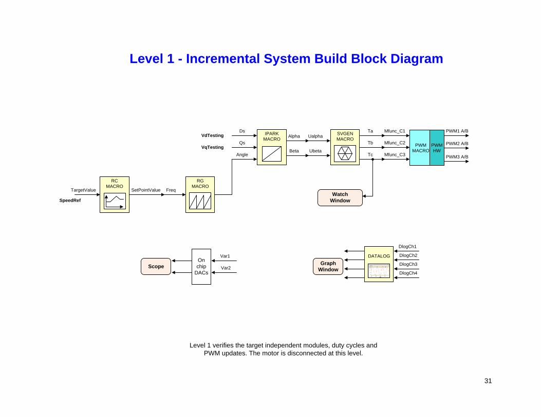
Level 1 - Incremental System Build Block Diagram

Level 1 verifies the target independent modules, duty cycles and

PWM updates. The motor is disconnected at this level.

ScopeGraph

Window

Alpha

Beta

IPARK

MACRO

Ds

Angle

Qs

VdTesting

VqTesting

TargetValue

RC

MACROSetPointValue

RG

MACROFreq

SpeedRef

Watch

Window

PWM

MACRO

PWM

HW

32

Level 1 Incremental Build

The block diagram of the system built in BUILDLEVEL 1 is shown in the previous page. At this step keep the motor disconnected. This section describes the steps for a “minimum” system check-out which confirms operation of system interrupt, the peripheral & target independent I_PARK_MACRO (inverse park transformation) and SVGEN_MACRO (space vector generator) modules and the peripheral dependent PWM_MACRO (PWM initializations and update) modules. Open MonoMtrServo-Settings.h and select level 1 incremental build option by setting the BUILDLEVEL to LEVEL1 (#define BUILDLEVEL LEVEL1). Now Right Click on the project name and click Rebuild Project. Once the build is complete click on debug button, reset CPU, restart, enable real time mode and run. If not already done, add variables to the expressions window by ‘Right Clicking’ within the Expressions Window and ‘Importing’ the file ‘variables_377sXL_DRV.txt’ from root directory. Set “EnableFlag” to 1 in the expressions window. The variable named “IsrTicker” will incrementally increase as seen in expressions window confirming that the interrupt is working properly. In the software, the key variables within the structure of ‘motor1’ to be adjusted are summarized below. SpeedRef : for changing the rotor speed in per-unit. VdTesting : for changing the d-qxis voltage in per-unit. VqTesting : for changing the q-axis voltage in per-unit. Level 1A (SVGEN_MACRO Test) The SpeedRef value is specified to the RG_MACRO module via RC_MACRO module. The IPARK_MACRO module is generating the outputs to the SVGEN_MACRO module. Three outputs from SVGEN_MACRO module are monitored via the graph window as shown in Figure 25 where Ta, Tb, and Tc waveform are 120

o apart from each other. Specifically, Tb lags Ta by 120

o and Tc leads Ta by

120o. Check the PWM test points on the board to observe PWM pulses (PWM-1H to 3H and PWM-1L

to 3L) and make sure that the PWM module is running properly.

Figure 25 Output of SVGEN, Ta, Tb, Tc and Tb-Tc waveforms

33

Level 1B (PWM_MACRO and INVERTER Test)

After verifying SVGEN_MACRO module in Level 1a, the PWM_MACRO software module and the 3-phase inverter hardware are tested by looking at the low pass filter outputs. Check VA-FB / VSENA, VB-FB / VSENB and VC-FB / VSENC test points using an oscilloscope. If you observe waveforms similar to what is shown in Level 1A, it ensures that the inverter is working properly.

After verifying this, take the controller out of real time mode (disable), reset the processor . Note that after each test, this step needs to be repeated for safety purposes, otherwise an improper shutdown might halt the PWMs at certain states where the inverter can draw high currents, hence caution need to be taken while doing these experiments

34

SVGEN

MACRO

PWM1 A/B

PWM2 A/B

PWM3 A/B

Mfunc_C1

Mfunc_C3

Mfunc_C2

Ta

Tc

Tb

Ualpha

Ubeta

Var1

Var2

On

chip

DACs

DATALOG

DlogCh1

DlogCh2

DlogCh3

DlogCh4

Level 2 - Incremental System Build Block Diagram

Scope

Graph

Window

Alpha

Beta

Ds

Angle

Qs

VdTesting

VqTesting

TargetValue

RC

MACROSetPointValue

RG

MACROFreq

PM

Motor

3-Phase

Inverter

PWM

MACRO

PWM

HW

Iph1 (Ia)

Iph2 (Ib)

Iph3 (Ic)

ADC

HW

_____

SDFM

HW

IPARK

MACRO

CLARKE

MACROResult0

Result1

As

Bs

Alpha

Beta

PARK

MACRO

Alpha

Beta

Out

ADC

code

________

SDFM

code

CurrentSensorSuite

QEP

SPEED FR

MACRO

ElecThetaPosition

Encoder

Suite

Speed

SpeedRpmQEP

Interface

Level 2 verifies the ADCs, offset compensation, SDFM, clarke / park transformations and position sensor interfaces.

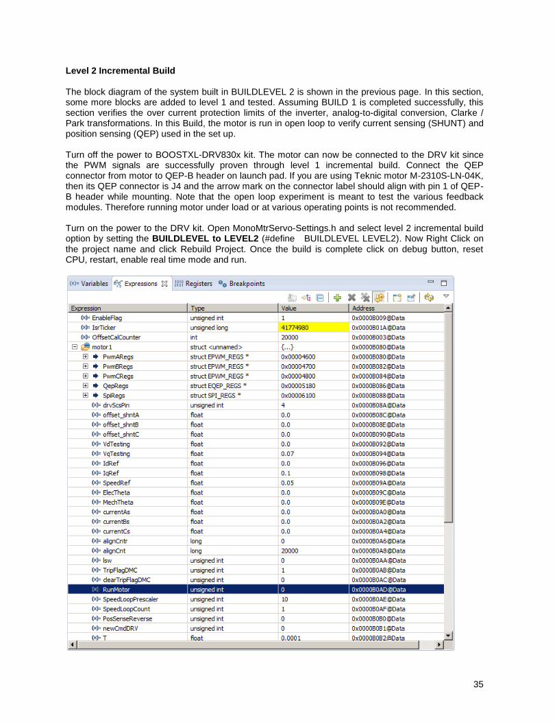
35

Level 2 Incremental Build The block diagram of the system built in BUILDLEVEL 2 is shown in the previous page. In this section, some more blocks are added to level 1 and tested. Assuming BUILD 1 is completed successfully, this section verifies the over current protection limits of the inverter, analog-to-digital conversion, Clarke / Park transformations. In this Build, the motor is run in open loop to verify current sensing (SHUNT) and position sensing (QEP) used in the set up. Turn off the power to BOOSTXL-DRV830x kit. The motor can now be connected to the DRV kit since the PWM signals are successfully proven through level 1 incremental build. Connect the QEP connector from motor to QEP-B header on launch pad. If you are using Teknic motor M-2310S-LN-04K, then its QEP connector is J4 and the arrow mark on the connector label should align with pin 1 of QEP-B header while mounting. Note that the open loop experiment is meant to test the various feedback modules. Therefore running motor under load or at various operating points is not recommended. Turn on the power to the DRV kit. Open MonoMtrServo-Settings.h and select level 2 incremental build option by setting the BUILDLEVEL to LEVEL2 (#define BUILDLEVEL LEVEL2). Now Right Click on the project name and click Rebuild Project. Once the build is complete click on debug button, reset CPU, restart, enable real time mode and run.

36

Figure 26 Expressions window for build level 2

Set “EnableFlag” to 1 in the expressions window. The variable “IsrTicker” will incrementally increase as seen in Expression window which confirms that the interrupt is working properly. In the software, the key variables within the structure of ‘motor1’ to be adjusted are summarized below. RunMotor : Set to 1 / 0 to start and stop motor SpeedRef : for changing the rotor speed in per-unit. VdTesting : for changing the d-qxis voltage in per-unit. VqTesting : for changing the q-axis voltage in per-unit. Now set “RunMotor” to 1 and the motor will start spinning after a few seconds. During open loop tests, VqTesting and SpeedRef should be adjusted carefully for PM motors so that the motor does not stall or vibrate. Phase 2A – Testing the Clarke module The three measured line currents are transformed to two phase alpha, beta currents in a stationary reference frame. The outputs of this module can be checked from graph window.

The clark1.Alpha waveform should be same as the clark1.As waveform.

The clark1.Alpha waveform should be leading the clark1.Beta waveform by 90o at the same

magnitude.

Since the low side current measurement technique is used employing shunt resistors on inverter phase

legs, the phase current waveforms sampled by ADC are composed of pulses as shown in Figure 28.

Figure 28 Amplified Phase A current

Figure 27 The waveforms of Svgen_dq1.Ta, rg1.Out, and phase A&B currents

37

Level 2B – Adjusting PI Limits

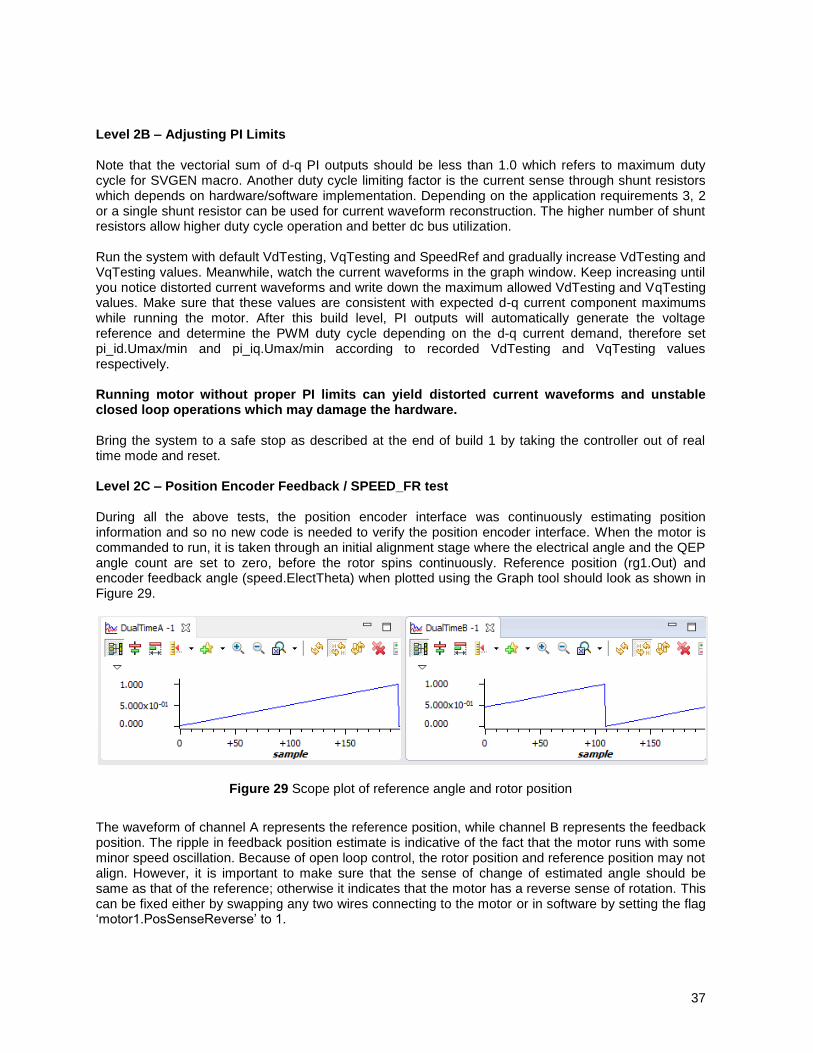
Note that the vectorial sum of d-q PI outputs should be less than 1.0 which refers to maximum duty cycle for SVGEN macro. Another duty cycle limiting factor is the current sense through shunt resistors which depends on hardware/software implementation. Depending on the application requirements 3, 2 or a single shunt resistor can be used for current waveform reconstruction. The higher number of shunt resistors allow higher duty cycle operation and better dc bus utilization. Run the system with default VdTesting, VqTesting and SpeedRef and gradually increase VdTesting and VqTesting values. Meanwhile, watch the current waveforms in the graph window. Keep increasing until you notice distorted current waveforms and write down the maximum allowed VdTesting and VqTesting values. Make sure that these values are consistent with expected d-q current component maximums while running the motor. After this build level, PI outputs will automatically generate the voltage reference and determine the PWM duty cycle depending on the d-q current demand, therefore set pi_id.Umax/min and pi_iq.Umax/min according to recorded VdTesting and VqTesting values respectively. Running motor without proper PI limits can yield distorted current waveforms and unstable closed loop operations which may damage the hardware. Bring the system to a safe stop as described at the end of build 1 by taking the controller out of real time mode and reset. Level 2C – Position Encoder Feedback / SPEED_FR test During all the above tests, the position encoder interface was continuously estimating position information and so no new code is needed to verify the position encoder interface. When the motor is commanded to run, it is taken through an initial alignment stage where the electrical angle and the QEP angle count are set to zero, before the rotor spins continuously. Reference position (rg1.Out) and encoder feedback angle (speed.ElectTheta) when plotted using the Graph tool should look as shown in Figure 29.

Figure 29 Scope plot of reference angle and rotor position

The waveform of channel A represents the reference position, while channel B represents the feedback position. The ripple in feedback position estimate is indicative of the fact that the motor runs with some minor speed oscillation. Because of open loop control, the rotor position and reference position may not align. However, it is important to make sure that the sense of change of estimated angle should be same as that of the reference; otherwise it indicates that the motor has a reverse sense of rotation. This can be fixed either by swapping any two wires connecting to the motor or in software by setting the flag ‘motor1.PosSenseReverse’ to 1.

38

To make sure that the SPEED_MACRO works fine, change the ‘motor1.SpeedRef’ variable in Expressions Window and check if the estimated speed variable ‘motor1.speed.Speed’ follows the commanded speed. Since the motor is a PM motor, where there is no slip, the running speed will follow the commanded speed regardless of the control being open loop.

With a QEP:

Watch out for ‘Qep1.CalibratedAngle’ in the Expressions window. It represents the electrical angle (or) position of rotor at the event of Index pulse. It can vary depending on starting position of rotor. When a closed loop operation is performed, it becomes important to ascertain the angular offset between electrical zero and QEP’s index pulse that would reset the QEP counter to zero. The calibration angle can be formulated as follows:

Calibration Angle = Offset Angle ± n . Line Encoder

39

Level 3 verifies the dq-axis current regulation performed by PI modules and speed measurement modules

SVGEN

MACRO

PWM1 A/B

PWM2 A/B

PWM3 A/B

Mfunc_C1

Mfunc_C3

Mfunc_C2

Ta

Tc

Tb

Ualpha

Ubeta

Alpha

Beta

Qs

Ds

IqRef

IdRef

TargetValue

RC

MACROSetPointValue

RG

MACROFreq

PM

Motor

3-Phase

Inverter

PWM

MACRO

PWM

HW

Iph1 (Ia)

Iph2 (Ib)

Iph3 (Ic)

IPARK

MACRO

CLARKE

MACROResult0

Result1

As

Bs

Alpha

Beta

PARK

MACRO

Alpha

Beta

SPEED FR

MACROElecTheta

Speed

SpeedRpm

Q_OutRef

PI

MACRO

Iq Reg

PI

MACRO

Id Reg

D_Out

Fbk

Ref

Fbk

OutSine/Cos

Ds

Qs

Constant 0lsw=0

lsw=1

Constant 0lsw=0

lsw=1

ADC

HW

_____

SDFM

HW

ADC

code

________

SDFM

code

CurrentSensorSuite

QEPPosition

Encoder

Suite

QEP

Interface

Level 3 - Incremental System Build Block Diagram

40

Level 3 Incremental Build Assuming the previous section is completed successfully, this section verifies the dq-axis current regulation performed by PI modules. To confirm the operation of current regulation, the gains of these two PI controllers are tuned for proper operation. In this build, transformations are done based on the reference angle generated manually rather than the actual rotor position. This is to ensure that this test can be done without a big load on the motor; otherwise Iq loop testing cannot be done easily. When the motor is commanded to run, it is taken through an initial alignment stage where the electrical angle and the QEP angle count are set to zero. Open MonoMtrServo-Settings.h and select level 3 incremental build option by setting the BUILDLEVEL to LEVEL3 (#define BUILDLEVEL LEVEL3). The user is free to pick any of the three supported CURRENT_SENSE methods. Now Right Click on the project name and click Rebuild Project. Once the build is complete click on debug button, reset CPU, restart, enable real time mode and run. Set “EnableFlag” to 1 in the expressions window. The variable “IsrTicker” will incrementally increase as seen in Expression window which confirms that the interrupt is working properly. In software, the key variables within the structure of ‘motor1’ to be adjusted are summarized below. RunMotor : Set to 1 / 0 to start and stop motor SpeedRef : for changing the rotor speed in per-unit. IdRef : for changing the d-qxis voltage in per-unit. IqRef : for changing the q-axis voltage in per-unit. In this build, the motor current is dynamically regulated by PI modules. The steps are explained as follows:

Compile/load/run program with real time mode.

Set SpeedRef to 0.3 pu (or another suitable value if the base speed is different), Idref to zero and Iqref to 0.05 pu (or another suitable value).

Expand ‘motor1’ to view variables ‘pi_id.Fbk’, ‘pi_id.Kp’ and ‘pi_id.Ki’ and corresponding elements for ‘pi_iq’ to the expressions window

Set ‘RunMotor’ flag to 1

Check pi_id.fbk in the expressions windows with continuous refresh feature and verify if it is tracking pi_id.Ref (IdRef). If not, adjust its PI gains properly.

Check pi_iq.fbk in the expressions windows with continuous refresh feature and verify if it is tracking pi_iq.Ref (IqRef). If not, adjust its PI gains properly.

To confirm these two PI modules, try different values of pi_id.Ref and pi_iq.Ref or SpeedRef.

For both PI controllers, the proportional, integral, derivative and integral correction gains may be re-tuned to have the satisfied responses.

Bring the system to a safe stop as described at the end of build 1 by taking the controller out of real time mode and reset. Now the motor will stop.

41

During running this build, the current waveforms in the CCS graphs should appear as follows*: * Deadband = 0.83 usec, Vdcbus=300V, dlog.trig_value=100

Figure 30 Measured theta, rg1.out and Phase A & B current waveforms

42

SVGEN

MACRO

PWM1 A/B

PWM2 A/B

PWM3 A/B

Mfunc_C1

Mfunc_C3

Mfunc_C2

Ta

Tc

Tb

Ualpha

Ubeta

Alpha

Beta

Qs

Ds

IqRef

IdRef

PM

Motor

3-Phase

Inverter

PWM

MACRO

PWM

HW

Iph1 (Ia)

Iph2 (Ib)

Iph3 (Ic)

IPARK

MACRO

CLARKE

MACROResult0

Result1

As

Bs

Alpha

Beta

PARK

MACRO

Alpha

Beta

ElecTheta

Speed

SpeedRpm

Q_OutRef

PI

MACRO

Iq Reg

PI

MACRO

Id Reg

D_Out

Fbk

Ref

Fbk

Sine/Cos

Ds

Qs

Constant 0 lsw=0

lsw=1

Constant 0 lsw = 0

Auto switched

from start

PI

MACRO

Spd Reg Spd_Out

Ref

Fbk

SpeedRef

lsw=2

ElecTheta lsw = 1, 2

ADC

HW

_____

SDFM

HW

ADC

code

________

SDFM

code

CurrentSensorSuite

QEPPosition

Encoder

Suite

QEP

Interface

SPEED FR

MACRO

Level 4 - Incremental System Build Block Diagram

Level 4 verifies the speed PI module and speed loop

43

Level 4 Incremental Build

Assuming the previous section is completed successfully; this section verifies the speed PI module and speed loop. All transformations are done based on the actual rotor position. When the motor is commanded to run, it is taken through an initial alignment stage where the electrical angle and the QEP angle count are set to zero. Open MonoMtrServo-Settings.h and select level 4 incremental build option by setting the BUILDLEVEL to LEVEL4 (#define BUILDLEVEL LEVEL4). Now Right Click on the project name and click Rebuild Project. Once the build is complete click on debug button, reset CPU, restart, enable real time mode and run. Set “EnableFlag” to 1 in the expressions window. The variable named “IsrTicker” will incrementally increase as seen in expressions window that confirms the interrupt working properly. In the software, the key variables of ‘motor1’ to be adjusted are summarized below. RunMotor : Set to 1 / 0 to start / stop motor SpeedRef : for changing the rotor speed (in per-unit). The key steps can be explained as follows:

Set Compile/load/run program with real time mode.

Set SpeedRef to 0.3 pu (or another suitable value if the base speed is different).

Set “RunMotor” to 1 to start the motor. The soft-switch variable (lsw) is auto promoted in a sequence depending on receipt of QEP index pulse.

- lsw=0, lock the rotor of the motor - lsw=1, motor in run mode and waiting for first instance of QEP Index pulse - lsw=2, motor in run mode, QEP - first Index pulse occurred

The motor will start running. Compare Speed with SpeedRef in the expressions windows with continuous refresh feature and verify that they are nearly the same.

To confirm this speed PID module, try different values of SpeedRef (positive or negative). For speed PID controller, the proportional, integral, derivative and integral correction gains may be re-tuned to get the desired response.

At very low speed range, the performance of speed response relies heavily on the fidelity of rotor position angle estimate provided by QEP encoder.

Bring the system to a safe stop as described at the end of build 1 by taking the controller out of real time mode and reset. Now the motor will stop.

44

During running this build, the current waveforms in the CCS graphs should appear as follows:

Figure 32 Measured theta, svgen duty cycle, and Phase A&B current waveforms under 0.33pu load & 0.3 pu speed

Figure 31 Measured theta, svgen duty cycle, and Phase A&B current waveforms under no-load & 0.3 pu speed

45

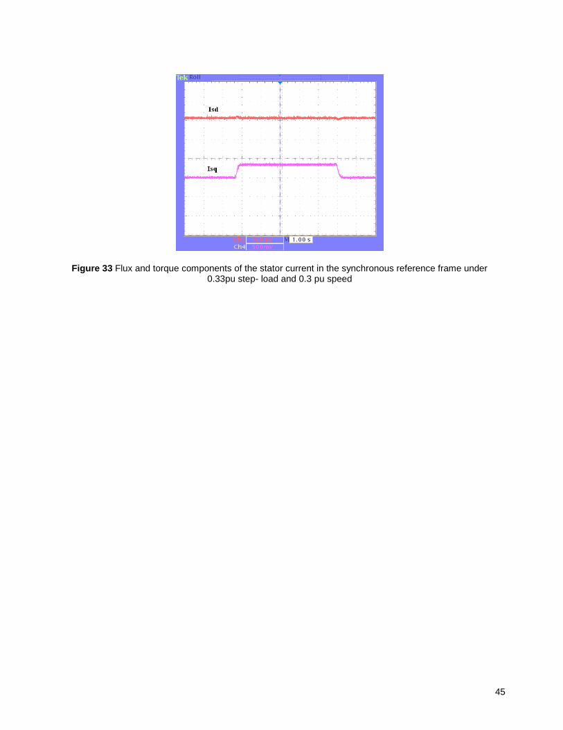
Figure 33 Flux and torque components of the stator current in the synchronous reference frame under 0.33pu step- load and 0.3 pu speed

46

Level 5 verifies the position PI module and position loop

SVGEN_MF

MACRO

PWM1 A/B

PWM2 A/B

PWM3 A/B

Mfunc_C1

Mfunc_C3

Mfunc_C2

Ta

Tc

Tb

Ualpha

Ubeta

Level 5 - Incremental System Build Block Diagram

Alpha

Beta

Qs

DsIdRef

PM

Motor

3-Phase

Inverter

PWM

MACRO

PWM

HW

IPARK

MACRO

CLARKE

MACROAs

Bs

Alpha

Beta

PARK

MACRO

Alpha

Beta

SPEED FR

MACROElecTheta

Direction

Speed

SpeedRpm

Q_OutRef

PI

MACRO

Iq Reg

PI

MACRO

Id Reg

D_Out

Fbk

Ref

Fbk

Sine/Cos

Ds

Qs

Constant 0 lsw=0

Constant 0lsw = 0

lsw => 0 to 1

Switched by

software, after an

alignment time lapse

‘alignCnt’

lsw => 1 to 2

Switched in software

when first index

pulse from QEP is

received

PI

MACRO

Spd Reg

Spd_Out

Ref

Fbk

SpeedRef

Lsw = 1 or 2

ElecThetalsw = 2

PI

MACRO

Pos Reg

Ref

Fbk

PositionRef

MechTheta

ADC

HW

_____

SDFM

HW

ADC

code

________

SDFM

code

CurrentSensorSuite

Iph1 (Ia)

Iph2 (Ib)

Iph3 (Ic)

Result0

Result1

QEPPosition

Encoder

Suite

QEP

Interface

47

Level 5 Incremental Build

This section verifies the position PI module and position loop with a QEP. For this loop to work properly, the previous section must have been completed successfully. When the motor is commanded to run, it is taken through an initial alignment stage where the electrical angle and the QEP angle count are set to zero. After ensuring a stable alignment, the rotor is spun in FOC from start. Open MonoMtrServo-Settings.h and select level 5 incremental build option by setting the BUILDLEVEL to LEVEL5 (#define BUILDLEVEL LEVEL5). Now Right Click on the project name and click Rebuild Project. Once the build is complete click on debug button, reset CPU, restart, enable real time mode and run. Set “EnableFlag” to 1 in the expressions window. The variable named “IsrTicker” will incrementally increase as seen in expressions windows confirming that the interrupt is working properly. Set ‘RunMotor’ to 1 in the Expressions window. Setting this flag will run the motor through predefined motion profiles / position settings as set by the ‘refPosGen()’ module. This module basically cycles the position reference through a set of values as defined in an array ‘posArray’. These values represent the number of the rotations/ turns with respect to the initial alignment position. Once a certain position value as defined in the array is reached, it will pause for a while before slewing towards the next one. Hence these array values can be referred as parking positions. During transition from one parking position to the next, the rate of transition (or speed) is set by ‘posSlewRate’. The number of positions in ‘posArray’ it will pass through before restarting again from the first value is decided by ‘ptrMax’. Hence add the variables “posArray”, “ptrMax” and “posSlewRate” to the expressions window. The key steps can be explained as follows:

Compile/load/enable real-time mode and run the program.

Add variables ‘pi_pos’, ‘posArray’, ‘ptrMax’ and ‘posSlewRate’ to the expressions window

Set RunMotor = 1 to run the motor. The motor should be turning to follow the commanded position (see note 1 below if the motor doesn’t turn properly).

The parking positions in ‘posArray’ can be changed to different values to see if the motor turns as many rotations as set.

The number of parking positions ‘ptrMax’ can also be changed to set a rotation pattern.

Position slew rate can be changed using ‘posSlewRate’. This represents the angle (in pu) per sampling instant.

The proportional and integral gains of the speed and position PI controllers may be re-tuned to get satisfactory responses. It is advised to tune the speed loop first and then the position loop.

Bring the system to a safe stop as described at the end of build 1 by taking the controller out of real time mode and reset. Now the motor will stop.

48

In the scope plot shown below, position reference and position feedback are plotted. It can be seen that they are aligned with negligible lag, which may be attributed to software. If the Kp, Ki gains of the position loop controller are not chosen properly, then it may lead to oscillations in the feedback or a lagged response.

Figure 34 Scope plot of reference position to servo and feedback position

NOTE:

1. If the motor response is erratic, then the sense of turn of motor shaft and the encoder may be opposite. Swap any two phase connections to the motor or set ‘motor1.PosSenseReverse’ to 1 and repeat the test.

2. The position control implemented here is based on an initial aligned electrical position (= 0). If the motor has multiple pole pairs, then this alignment can leave the shaft in different mechanical positions depending on the pre start mechanical position of rotor. If mechanical position repeatability or consistency is needed, then QEP index pulse should be used to set a reference point. This may be taken as an exercise.

3. With an absolute encoder like resolver/ EnDAT/ BiSS, the above may not be an issue as the resolver gives unique angular value for each position.