sensorimotor adaptation to perturbations of vowel

Sensorimotor Adaptation to Perturbations of Vowel Acoustics and its Relation to Perception

By

Virgilio Mangubat Villacorta

B.S., Physics with Specialization in Biophysics

University of California, San Diego, 1995

SUBMITTED TO THE HARVARD-MIT DIVISION OF HEALTH SCIENCES AND TECHNOLOGY

IN PARTIAL FULFILLMENT OF THE REQUIREMENTS FOR THE DEGREE OF

DOCTOR OF PHILOSOPHY IN

SPEECH AND HEARING BIOSCIENCE AND TECHNOLOGY AT THE

MASSACHUSETTS INSTITUTE OF TECHNOLOGY

FEBRUARY 2006

Copyright © 2006 Virgilio Villacorta. All rights reserved.

The author hereby grants MIT permission to reproduce and to distribute publicly paper and electronic copies of this thesis document in whole or in part.

Signature of Author ________________________________________________

Harvard-MIT Division of Health Sciences and Technology

September 19, 2005 Certified by_______________________________________________________

Joseph S. Perkell, D.M.D., Ph.D. Senior Research Scientist, Research Laboratory of Electronics

Harvard-MIT Division of Health Sciences and Technology Thesis Supervisor

Accepted by______________________________________________________

Martha L. Gray, Ph.D. Edwin Hood Taplin Professor of Medical and Electrical Engineering

Co-Director, Harvard-MIT Division of Health Sciences and Technology

2

This page intentionally left blank.

3

Acknowledgements

I would like to start by thanking the members of my committee for their sage

advice. My deepest gratitude goes to my advisor and friend, Joe Perkell, without

whose constant support and guidance I would not have been able to start—let

alone finish—this work. Along with Joe, I am also greatly indebted to Frank

Guenther, who has also spent innumerable hours guiding me on this project from

its inception. I am also grateful for the valuable feedback I received from Tom

Quatieri and Steve Massaquoi, and for the time they have spent reading and

discussing with me the various drafts of this work.

Over these past six years, I feel like I’ve asked for advice or help from every

member of the speech communications group at one point or another. I

especially want to thank Ken Stevens for his insight as chair of my oral qualifying

exam committee; Majid Zandipour, for helping me get the SA project off the

ground; Mark Tiede, for developing a comprehensive set of Matlab tools that

made my life so much easier; and Satra Ghosh, for always having an answer

ready to my random queries. I also want to thank Arlene Wint; I think the lab

would fall apart without you. To the people I’ve shared an office with—Laura

Dilley, Xuemin Chi, Tony Okobi, and Xiaomin Mou: thanks for listening to my

rantings, and letting me throw things at/with you. And to the remaining friends

I’ve made in the speech group—Harlan Lane, Stephanie Shattuck-Hufnagel,

Janet Slifka, Nicole Marrone, Ellen Stockmann, Steven Lulich, Kushan Surana,

Annika Imbrie, Lan Chen, Neira Hajro, Seth Hall, Sharon Manuel, Melanie

Matthies, Helen Hanson, Nancy Chen, Margaret Denny and others: thanks for

sharing good times, intriguing conversation and the occasional libation.

My life at MIT was also shaped substantially by things I did outside the lab. I

would like to recognize the following friends I’ve made along the way: my former

roommates (Martin McKinney, Leonardo Cedolin, Mia Kiistala, Milena

Virrankoski, Petra Aminoff, Sandrine Arnaud, Edward Ha, and Nigela Xhamo);

4

fellow members of the Graduate Student Council (especially Emmi Snyder,

Barun Singh, Hector Hernadez, Lucy Wong, and Jess Vey); fellow soldiers

(especially Colonel Michael Brennan); and fellow grad students (especially Tim

Wagner, Zach Smith, and Dan Shub). Thank you all for making the time I spent

at MIT an adventure. Thanks as well to lifelong friends who have made my entire

life an adventure: Don Gurskis, Arlene Yang, Clinton Yee, Chuck Nguyen, Josh

Burrell, Monika Garcia, and Julie Ting.

Above all, I would like to thank my family. I could not have completed this work

without the lifetime of support and dedication from Mom and Dad; the

encouragement from my sisters, Estella and Genie; and the love and

companionship of my partner in life, Jenny.

* * * * * * * * * * *

This work has been supported by the National Institute of Deafness and

Communication Disorders Grant R01-DC01925, and by the Harvard-MIT Division

of Health Science and Technology.

* * * * * * * * * * *

I dedicate this work to the memory of my father.

5

Sensorimotor Adaptation to Perturbations of Vowel Acoustics and its Relation to Perception

By

Virgilio Mangubat Villacorta

Submitted to the Division of Health Sciences and Technology

on September 19, 2005 in Partial Fulfillment of the Requirements of the Degree of Doctor of Philosophy in

Speech and Hearing Bioscience and Technology Abstract The overall goal of this dissertation was to study the auditory component of feedback control in speech production. The first study investigated auditory sensorimotor adaptation (SA) as it relates to speech production: the process by which speakers alter their speech production in order to compensate for perturbations of normal auditory feedback. Specifically, the first formant frequency (F1) was shifted in the auditory feedback heard by naive adult subjects as they produced vowels in single syllable words. These results indicated that subjects demonstrate compensatory formant shifts in their speech. This compensation was maintained when auditory feedback was masked by noise. The second study investigated perceptual discrimination of vowel stimuli differing in F1 frequency, using the same subjects as in the SA studies. This study showed that the extent of adaptation was positively correlated with subject auditory acuity. The last study consisted of a series of simulations of SA experiments using a model which describes the motor planning and control of human speech by the brain; these simulations showed that the model can account for several properties of adaptation as measured from the human subjects. The findings in this dissertation support the idea that phonemic speech movements are planned as goal regions in an auditory space, and that mappings between this auditory space and the speech motor plan are adaptable. Moreover, the size of these goal regions—as reflected in speaker auditory acuity—influences the degree to which speakers adapt to errors in auditory feedback. Thesis Supervisor: Joseph S. Perkell Title: Senior Research Scientist, Research Laboratory of Electronics

6


7

TABLE OF CONTENTS

Chapter 1. Introduction. ...................................................................................17

1.1. Organization of this thesis. .......................................................................18

Chapter 2. Sensorimotor adaptation and the motor control of speech. ......19

2.1. Sensorimotor adaptation and sensorimotor control ..................................19

2.2. Feedback and feedforward motor control mechanisms............................22

2.3. An overview of a model for the motor planning of speech (DIVA). ...........25

Chapter 3. Sensorimotor adaptation (SA) to acoustic perturbations in the first formant of vowels and relation to vowel spacing (Study 1). .................30

3.1. Review of past formant perturbation SA experiments ..............................30

3.2. Specific hypotheses of the sensorimotor adaptation experiment..............33

3.2.1. Adaptation properties measured in voiced speech. ...........................33

3.2.2. Aftereffect adaptation.........................................................................34

3.2.3. Adaptation specificity. ........................................................................34

3.2.4. Contribution of F0 to adaptation.........................................................35

3.2.5. Within token adaptation. ....................................................................36

3.3. Methodology of study 1: the sensorimotor adaptation (SA) experiment. .37

3.3.1. Minimal delay formant shift in voiced speech.....................................37

3.3.2. Experimental design and protocol for SA training. .............................40

3.3.3. Subject selection criteria and description...........................................44

3.3.4. Vowel formant and F0 extraction. ......................................................44

3.3.5. Rejection of an SA subject from analysis based on produced F1. .....45

3.4. Results and analysis of the sensorimotor adaptation experiment.............46

3.4.1. Adaptive Response Index. .................................................................49

3.4.2. Analysis of +feedback adaptation. .....................................................51

3.4.3. Analysis of –feedback adaptation for the vowel /ε/. ...........................55

3.4.4. Analysis of generalized adaptation for multiple vowels. .....................59

3.4.5. Analysis of the contribution of F0 to adaptation. ................................64

3.4.6. Analysis of within token adaptation. ...................................................66

8

3.5. Study 1 summary. ....................................................................................69

Chapter 4. Cross-correlation comparison between vowel discrimination and SA (study 2). ......................................................................................................70

4.1. Background and specific aims of the perceptual acuity experiment. ........70

4.1.1. Relation between vowel discrimination and adaptation. ....................70

4.1.2. Relation between vowel spacing and adaptation. ..............................73

4.2. Methodology of study 2: the perceptual acuity experiment......................74

4.2.1. Participating subjects. ........................................................................75

4.2.2. Recording of the subject’s speech. ....................................................75

4.2.3. Staircase protocol to estimate jnd. .....................................................76

4.2.4. A more precise same-different protocol. ............................................77

4.2.5. Goodness rating task. ........................................................................78

4.3. Analysis and correlation results................................................................79

4.3.1. Analysis of d’ scores. .........................................................................79

4.3.2. Correlation between jnd scores and adaptation scores. ....................80

4.3.3. Correlation between vowel F1 separation and adaptation scores......85

4.3.4. Correlation between perceptual acuity measure and adaptive

response, when adjusting for dependence on vowel separation..................88

4.3.5. Analysis of goodness rating data. ......................................................91

4.3.6. Correlation between goodness rating error and adaptive response...94

4.4. Study 2 summary .....................................................................................96

Chapter 5. SA simulations utilizing the DIVA model (Study 3). ....................97

5.1. Outline of the DIVA model and overview of the SA simulations. ..............97

5.1.1. A Functional Outline of the DIVA model.............................................97

5.1.2. Sensory goal regions and auditory acuity in the DIVA model. .........100

5.1.3. Design of the SA simulations within the DIVA model. ......................105

5.2. DIVA SA simulations results, with comparison to human subject

experiments...................................................................................................108

5.2.1. DIVA simulations compared with human subject experiments in the

+feedback condition...................................................................................108

9

5.2.2. DIVA simulations changes with changes in simulation parameters. 110

5.2.3. Changes in the second formant frequency found in the DIVA SA

simulations.................................................................................................113

5.2.4. DIVA simulations compared to human subject results in the blocked

feedback condition.....................................................................................115

5.2.5. Comparison with a simple conceptualization of the auditory goal

regions (the “all or nothing” approach).......................................................117

5.3. Study 3 Summary...................................................................................120

Chapter 6. Overall summary and future directions......................................123

6.1. Overall research summary. ....................................................................123

6.2. The role of somatosensory feedback. ....................................................123

6.3. SA experiments using acoustic perturbations of other acoustic cues.....124

6.4. Neuroanatomic loci of sensory error cells. .............................................125

6.5. Proposed enhancements to the DIVA model..........................................126

Appendix A. Summary of terms used in this thesis. ...................................128

Appendix B. Use of the LPC coefficients to determine and shift F1. .........129

Appendix C. Individual adaptive response during the sensorimotor adaptation protocol. .......................................................................................134

Appendix D. Investigation of the influence of the perturbation algorithm on the second formant.........................................................................................138

Appendix E. Correlation between adaptive response and jnd obtained from staircase protocol only...................................................................................139

Appendix F. Relation between category width and adaptive response. ....141

Bibliography....................................................................................................145

Biographical Note ...........................................................................................150

10

TABLE OF FIGURES Figure 2.1: The feedback control system. ..........................................................23

Figure 2.2: Two simple control schemes that involve internal models. ..............24

Figure 2.3: Feedback error learning motor control scheme. ..............................24

Figure 2.4: Sensory expectations or goals are encoded by the projections from

premotor cortex (P) to auditory and somatosensory error cells (ΔAu and ΔS), and

contain cortico-cortical and cerebellar components ............................................27

Figure 2.5: Projections from the auditory and somatosensory error cells (ΔAu

and ΔS) to motor cortex (M) form the feedback controller ..................................27

Figure 2.6: Projections (directly and via the cerebellum) from premotor cortex (P)

to primary motor cortex (M) form the feedforward controller. ..............................28

Figure 2.7: Relation between perceptual acuity and contrast distance for two

hypothetical phonemes X and Y. ........................................................................29

Figure 3.1: Feedback transformation used in the Houde and Jordan SA speech

experiment. .........................................................................................................32

Figure 3.2: Idealized example of within token adaptation. .................................36

Figure 3.3: Formant shifting algorithm used to introduce acoustic perturbation in

SA experiment ....................................................................................................39

Figure 3.4: Outline of the cycle that occurred during the presentation of one

token during the SA experiment..........................................................................41

Figure 3.5: Diagram of the level of first formant perturbation presented during

one experimental session, as a function of epoch number. ................................43

Figure 3.6: Percentage of tokens with F1 outside the window of frequencies

which is shifted by the DSP algorithm.................................................................46

Figure 3.7: Produced first formants, normalized to the mean baseline value, in

+feedback words for all subjects.........................................................................47

Figure 3.8: Produced first and second formant frequencies, normalized to the

adjusted baseline, in +feedback words for all subjects .......................................48

Figure 3.9: Adaptive response (AR) compared between 0.7 pert (black line) and

1.3 pert (dark gray) subjects ...............................................................................50

11

Figure 3.10: Adaptive response (AR) for the first formant in +feedback words for

all subjects. .........................................................................................................52

Figure 3.11: Adaptive response (AR) for the second formant in +feedback words

for all subjects. ....................................................................................................53

Figure 3.12: Mean adaptive response in F2 (ARF2) as a function of mean

adaptive response in F1 (ARF1), for ramp phase through post-pert epochs........54

Figure 3.13: Mean adaptive response in F2 (ARF2) as a function of mean

adaptive response in F1 (ARF1), for baseline epochs..........................................55

Figure 3.14: Adaptive response (AR) for the first formant of the –feedback token

“pet” (the same context token) for all subjects exposed to 0.7 pert in F1............56

Figure 3.15: Adaptive response (AR) for the first formant of the –feedback token

“get” and “peg” combined (the different context tokens) for all subjects exposed

to 0.7 pert in F1...................................................................................................58

Figure 3.16: Shift in F1/F2 vowel space for all vowels of the -feedback tokens,

0.7 pert female subjects......................................................................................61


0.7 pert male subjects.........................................................................................62


1.3 pert female subjects......................................................................................62


1.3 pert male subjects.........................................................................................63

Figure 3.20: F0 normalized to the mean of the baseline epochs (1-15), as a

function of epoch number. ..................................................................................65

Figure 3.21: Correlation between normalized F0 difference and the normalized

F1 difference, over the full pert epochs...............................................................66

Figure 3.22: Example of time segmentation of tokens for within-vowel

adaptation. ..........................................................................................................67

Figure 3.23: Segmental adaptive response for the front and end vowel segments

during the entire SA protocol. .............................................................................68

Figure 4.1: The auditory goal region. .................................................................71

12

Figure 4.2: Proposed relation between auditory goal region size and adaptive

response .............................................................................................................72

Figure 4.3: Proposed relation between vowel spacing and adaptation ..............74

Figure 4.4: Example an adaptive rocedure used to estimate jnd .......................77

Figure 4.5: Token pairs used within the more precise same-different protocol.. 78

Figure 4.6: Example of calculating jnd more precisely from the “same-different”

d’ scores .............................................................................................................80

Figure 4.7: Adaptive response index is not correlated with the jnd score of the

milestone in the same direction as the SA training .............................................83

Figure 4.8: Adaptive response index is correlated with the jnd score of the center

milestone.. ..........................................................................................................84

Figure 4.9: Adaptive response index is not correlated with the jnd score of the

milestone in the opposite direction of the SA training. ........................................84

Figure 4.10: Adaptive response index is not correlated with the baseline vowel

F1 separation on the same side as the perturbation ...........................................86

Figure 4.11: Adaptive response index is not correlated with the baseline vowel

F1 separation on the opposite side of the perturbation. ......................................86

Figure 4.12: Adaptive response index—excluding negative ARI—is correlated

with the baseline vowel F1 separation on the same side as the perturbation. ....87

Figure 4.13: Adaptive response index, normalized by produced vowel separation

in F1, is correlated with the jnd score of the center milestone. ...........................91

Figure 4.14: Example of the analysis of the goodness rating task in one subject.

............................................................................................................................92

Figure 4.15: Analysis of the goodness rating task for outlier subject 1 ..............93

Figure 4.16: Analysis of the goodness rating task for outlier subject 2. .............93

Figure 4.17: Adaptive response index is correlated with total goodness rating

standard error .....................................................................................................95

Figure 5.1: A functional outline of the DIVA model.............................................97

Figure 5.2: Example of the hypothetical activation distributions, in an auditory

dimension .........................................................................................................102

13

Figure 5.3: Relation between subject adaptive response index (ARI) and model

σF value.............................................................................................................104

Figure 5.4: Normalized F1 during the SA protocol (with feedback), DIVA

simulations compared to human subject results. ..............................................109

Figure 5.5: Adaptive response (AR) in F1 during the SA protocol (with feedback),

DIVA simulations compared to human subject results. .....................................110

Figure 5.6: Adaptive response (AR) in F1 if the learning rate of the

somatosensory goal zPS is increased ..............................................................111

Figure 5.7: Adaptive response (AR) in F1 decreases if the contribution of

auditory feedback relative to somatosensory feedback is decreased. ..............112

Figure 5.8: Adaptive response in F2 during the SA protocol (with feedback),

DIVA simulated subjects compared to human subject results ..........................113

Figure 5.9: Normalized F1 in SA results and simulations, from tokens with

feedback, using Miller ratio auditory dimensions. .............................................114

Figure 5.10: Adaptive response of F2 in SA results and simulations, from tokens

with feedback, using Miller ratio auditory dimensions. ......................................115

Figure 5.11: Adaptive response (AR) in F1 for blocked feedback trials, DIVA

simulated subjects compared to human subject results....................................116

Figure 5.12: Adaptive response in blocked auditory feedback tokens changes

with changes in zPMlearning_rate ...........................................................................116

Figure 5.13: Dependence of the output of auditory error cells on the size of the

auditory goal. ....................................................................................................118

Figure 5.14: Normalized F1 during the SA protocol (with feedback) using “all or

nothing” auditory goal regions...........................................................................119

Figure 5.15: Comparison of normalized F1 during the early part of the ramp-

phase between simulations using goal regions that are Gaussian (left) or “all or

nothing” (right)...................................................................................................120

Figure B.1: Graphic depiction of the roots (polar form) corresponding to the

original and perturbed speech segments ..........................................................131

Figure B.2: DFT spectrum within an example /ε/ vowel, unperturbed. .............132

Figure B.3: DFT spectrum within an example /ε/ vowel, perturbed. .................133

14

Figure C.1: Individual adaptive response as a function of epoch number for 0.7

pert SA protocol, female subjects. ....................................................................134


pert SA protocol, male subjects ........................................................................135


pert SA protocol, female subjects. ....................................................................136


pert SA protocol, male subjects ........................................................................137

Figure E.1: Adaptive response index is not correlated with the 1-stage estimate

of the jnd for the center milestone.....................................................................140

Figure F.1: Example of the calculation of category width from the goodness

rating scores .....................................................................................................141

Figure F.2: Adaptive Response Index (ARI) is not correlated with the category

width as determined from the normalized goodness rating scores. ..................142

15

LIST OF TABLES Table 3.1: Tokens presented to the subject during the SA experiment..............42

Table 3.2: Summary of adaptive response index (ARI) calculated in study 1. ...59

Table 4.1: Partial correlation coefficients, using F1 vowel separation

corresponding to the same side of the perturbation ............................................89

Table 4.2: Partial correlation coefficients, using F1 vowel separation

corresponding to the opposite side of the perturbation. ......................................90

Table 5.1: Relevant DIVA parameter for the SA simulation .............................107

Table E.1: Statistics of correlation between ARI and jnd, one-stage protocol

estimate of jnd compared to two-stage protocol jnd measure...........................140

Table F.1: Correlation coefficients between category width and adaptive

response index (ARI) with p-values for a range of criterion values ...................143

Table F.2: Comparison between p-values for correlation coefficients between

category width and ARI scores, zero-order correlation compared to the partial

correlation with F1 separation controlled for. ....................................................144

16


17

Chapter 1. Introduction.

This dissertation investigates the role of sensory feedback in the motor planning

of speech, and specifically focuses on speech sensorimotor adaptation.

Sensorimotor adaptation is an alteration of a motor task that results from the

alteration of sensory feedback; psychophysical experiments that present human

subjects with altered sensory environments have revealed the relationship of

sensory feedback to motor control in both non-speech and speech contexts.

Experiments on limb movements have demonstrated the influence of

proprioceptive feedback—i.e. feedback pertaining to limb orientation and

position—(Bhushan and Shadmehr, 1999; Blakemore et al., 1998)—and visual

feedback (Bedford, 1989; Welch, 1978). Feedback-modification studies have

also been conducted on speech production, including a number of studies that

have induced compensation by altering the configuration of the vocal tract in

some way (Abbs and Gracco, 1984; Lindblom et al., 1979; Savariaux et al.,

1995). Other experiments have investigated speech adaptation to novel acoustic

feedback, such as delayed auditory feedback (Yates, 1963) or changes in

loudness (Lane and Tranel, 1971). Several studies of sensorimotor adaptation

have investigated responses based on real-time alterations of the perceived pitch

of vowel sounds (Kawahara, 1993; Xu et al., 2004) and a limited number have

shown compensatory responses to real-time modifications of vowel formant

structure (Houde and Jordan, 1998; Max et al., 2003).

The series of studies reported here investigate acoustic speech sensorimotor

adaptation resulting from perturbations of specific vowel formant frequencies,

and how this adaptation relates to vowel perception in cross-subject correlation

studies. The data obtained from these experiments are compared to results from

simulations from a well developed neural network model of speech motor

planning, the DIVA (Directions Into Velocities of Articulators) model (Guenther

and Ghosh, 2003).

18

1.1. Organization of this thesis.

Following this introduction, chapter 2 summarizes relevant research in the field of

sensorimotor adaptation and sensorimotor control, with a focus on relevance to

speech motor control and the DIVA model. Chapter 3 presents the results of

study 1, an experiment that measured sensorimotor adaptation in response to

acoustic perturbations in the first formant of vowels. Chapter 4 describes study

2, in which subjects’ perceptual acuity to the acoustic perturbation was measured

and related to the extent of their adaptive response in study 1. Chapter 5

describes study 3, which compared the results from studies 1 and 2 with

simulations using the DIVA model. Finally, chapter 6 suggests future directions

for studies of speech motor control using acoustic sensorimotor adaptation.

19

Chapter 2. Sensorimotor adaptation and the motor control of speech.

The motor control of speech—the manner in which the brain commands the

vocal tract to produce speech—has been one of the longest studied aspects of

the speech communication process. Issues related to speech motor control

include speech acquisition, adaptation to changes during normal human growth

and development, and adjustment to novel conditions (both pathological and

experimentally induced). Work in this field has benefited immensely from the

parallel progress made in non-speech sensorimotor control—the study of how

the brain incorporates sensory information to guide movements in order to

achieve some desired goal or outcome. Additional understanding of speech

motor control has been derived from the use of neural network models such as

the DIVA model (Guenther et al., 2005). Such models incorporate and expand

upon many theories that have resulted from the general study of sensorimotor

control to develop a cohesive and neuro-anatomically valid model that account

for how the brain accomplishes the extremely complicated task of controlling the

articulatory movements of speech production.

2.1. Sensorimotor adaptation and sensorimotor control

One way of investigating the relationship between sensory information and the

control of motor movements is to modify the sensory feedback available to a

subject, then measure the manner and degree to which that subject alters motor

movements in response. Such a change in movements in response to distorted

sensory feedback is termed sensorimotor adaptation (SA). Before investigating

the relationship of acoustic feedback to the motor control of speech, it is useful to

understand SA findings in a somewhat analogous task: that of visual feedback to

the motor control of reaching. This visual-reaching relation has been well

characterized by wedge prism adaptation experiments (von Helmholtz, 1962). In

these experiments, subjects wore prism glasses that altered their visual field. In

compensatory responses, the subjects changed movement behavior in a way

20

that was consistent with a temporary modification of neural mappings relating

their visual perception to motor commands. Moreover, when the prism glasses

were removed, these subjects demonstrated aftereffect adaptation: temporary

retention of compensatory movements once the visual input was returned to

normal.

Such SA experiments have been useful in demonstrating the dependence of

reaching movements on visual feedback. For example, the aforementioned

experiments utilizing visual-field shifting prism glasses have demonstrated that

the visuomotor system is plastic, and can adapt to a number of perturbations

(Welch, 1978). A modern equivalent version of the prism paradigm—using a

computer to visually altered the perceived location of the finger during a pointing

task—has also demonstrated visuomotor remapping that compensates for an

alteration azimuth position (Bedford, 1989). Variant experiments of this

perturbed pointing task—designed to cause two-dimensional visuomotor

adaptation—have also shown visuomotor remappings that generalized greatest

at the site of perturbation and decayed away from it (Ghahramani et al., 1996).

The results of these experiments—and other related visuomotor SA

experiments—led to the inference that reaching movements rely on neural

mappings that relate sensory (visual) feedback to motor commands. Moreover,

the latter experiments (Bedford, 1989; Ghahramani et al., 1996)—which visually

altered the finger location via a computer—provided the inspiration to the design

of a speech SA experiment, discussed below (Houde and Jordan, 1998).

Some adaptation-inducing experiments performed in the domain of speech

include experiments that alter the vocal tract in some persistent way, such as

compensation in vowel productions found when the position of the mandible is

fixed with a bite-block (Lindblom et al., 1979), compensatory tongue movements

in production of the vowel /u/ when the lip opening is fixed with a lip tube

(Savariaux et al., 1995; Savariaux et al., 1999), and adaptations found in /s/

productions in response to the introduction of an artificial palate (Baum and

21

McFarland, 1997). There are also a number of speech experiments in which

some aspect of somatosensory sensation1 is blocked or altered by the

unexpected perturbations of some aspect of movement. These include the

compensatory orofacial muscle responses that were induced by unanticipated

load perturbations on the lips during speech (Abbs and Gracco, 1984),

compensatory responses due to unexpected perturbations of the palate shape

(Honda et al., 2002), or in jaw movement (Tourville et al., 2004). Such

compensation experiments have demonstrated the reliance of speech on

somatosensory feedback from the articulators involved in speech. In particular,

the palatal shape perturbation study (Honda et al., 2002) highlights adaptation to

specific somatosensory feedback perturbations and is the only work referenced

above which combines articulator perturbation with masking noise, thereby

separating the effects of somatosensory feedback from auditory feedback.

Feedback-modification experiments using acoustic perturbations have also been

used to understand how speech production is influenced by auditory feedback.

Early research in this field was limited to modifying the amplitude of speech

auditory feedback—showing that normal subjects spoke louder when their

perceived loudness was decreased (Lane and Tranel, 1971; Yates, 1963)—or to

delays in acoustic feedback—showing that fluent speech production is seriously

impaired by small time delays in hearing one’s own voice (Yates, 1963). With the

advent of digital signal processing (DSP), researchers have been able to make

near real-time (i.e. short time delay) adjustments to the spectral content of

speech. DSP has been used in pitch-shift experiments, in which the fundamental

frequency (F0) of sustained vowels was raised or lowered in subjects’ auditory

feedback (Burnett et al., 1998; Jones and Munhall, 2000; Kawahara, 1993).

When F0 shifts were introduced during production of tonal sequences in

Mandarin (a tone language), subjects responded with compensatory F0 shifts in

the opposite direction, with delays as short as 150 msec (Xu et al., 2004).

1 Somatosensory sensation generally refers to the perception of sensory stimuli from the skin and internal organs. In the context of speech motor control, somatosensory sensation refers to the perception of stimuli—tactile and positional information—from the vocal tract organs.

22

Some researchers have specifically investigated the sensorimotor adaptation

when the feedback of the spectral content of a subject’s speech is perturbed in

nearly real-time (Houde and Jordan, 1998; Max et al., 2003). All these feedback

modification experiments have found compensatory responses which show the

strong influence of acoustic feedback on speech motor control. These latter two

experiments are discussed in further detail in Section 3.1.

2.2. Feedback and feedforward motor control mechanisms.

The aforementioned evidence showing specific compensatory adjustments of

speech parameters in response to sensory feedback perturbations indicates that

movements make use of feedback control mechanisms. In feedback control

systems, the output of the plant (that is, the controlled object) is fed back to the

controller, so that this feedback signal can be incorporated into the command

produced by the controller. Typically, the signal output by the controller is the

error (that is, the difference between the input and feedback signal), weighted by

a gain factor. (Refer to Figure 2.1) the amount of gain used in the controller

plays a principal role in determining how quickly a system adapts to change, as

well as how stable that system is. While potentially simple in design, high-

performance feedback control systems may require large loop gains (Sinha,

1994). Given the signal transmission and processing delays in biological neural

systems, one potential risk of feedback control loops is instability (Ito, 1974).

23

Figure 2.1: The feedback control system. (a) The controller governs the plant (i.e. the controlled object), utilizing feedback information from the output of the plant. (b) A simple implementation of a feedback control system, in which the controller generates an error signal from the feedback and input, and weighs (with gain) the resulting signal appropriately.

Instabilities that may result in feedback control can be avoided by feedforward

control. Since feedforward control does not rely directly on feedback input, it can

operate without the delays of feedback loops and thus at higher gains. To

operate in a feedforward mode, motor control systems make use of internal

models—neural representations that mimic the behavior of the motor system

(Miall and Wolpert, 1996). Specifically, internal models allow feedforward control

by predicting the sensory feedback that is used in a feedback controller—the

forward model (see Figure 2.2a)—or by directly predicting the desired motor

command that results in the desired state—the inverse model (see Figure 2.2b).

One major problem with a feedforward controller is that internal models must

somehow learn to make accurate predictions; moreover, the predictions of

internal models are not accurate in the presence of unexpected perturbations.

CONTROLLER PLANT

FEEDBACK

OUTPUT

PLANT OUTPUT ∑ INPUT

- +

GAIN

CONTROLLER

(a)

(b)

24

PLANT STATEDesired STATE -

+ CONTROLLER

(a) FORWARD MODEL

PLANT STATEDesired STATE

(b)

INVERSE MODEL

Figure 2.2: Two simple control schemes that involve internal models. a) A forward model predicts the expected feedback from the output state, and can replace the actual feedback without its inherent delays. b) An inverse model can directly predict the control commands that act on the plant to achieve the desired state. (Miall and Wolpert, 1996).

The feedback error learning control scheme (Kawato and Gomi, 1992) takes

advantage of the beneficial properties of feedback and feedforward control by

using both types of controllers into to determine the overall motor command (see

Figure 2.3). In particular, the overall command in this control scheme is the

summation of the computed feedforward component and the feedback

component; the feedback command is also used to train the inverse model,

which is used to calculate the feedforward command. The DIVA model utilizes a

similar control scheme to explain the motor planning of speech.

FeedbackControllerDesired

movement -+

Inverse ModelFeedforward Controller

Plant Realizedmovement+

+

Motor command

Figure 2.3: Feedback error learning motor control scheme. This control scheme sums both the feedback controller component and the feedforward controller component (the inverse model), yielding the motor command and eventually the realized movement. The output of the feedback controller is used to train the feedforward controller (dashed line). (Kawato and Gomi, 1992).

25

Before discussing a model of speech motor planning in detail, it is helpful to

clarify some of the terminology, especially as it relates to the larger body of motor

control research. Theories of motor control often distinguish between kinematic

control—which refers to the control of the position and velocities of the controlled

object—and dynamic control—which refers to the control of the forces needed to

move the controlled object—(Atkeson, 1989). While kinematic and dynamic

theories of motor control can be used within the same control scheme—including

speech motor planning (Perkell et al., 2000)—the DIVA model discussed below is

largely a kinematic one. Such approaches assume that the dynamic control

factors are relatively unimportant. This assumption is based on observations that

the masses of most vocal tract structures (articulators) are small, and the

maximum forces generated by articulator muscles are generally much greater

than needed in speech movements2. Internal models involving dynamic motor

control have also been studied extensively (Kawato, 1999), but are beyond the

scope of the current investigation.

2.3. An overview of a model for the motor planning of speech (DIVA).

One promising line of modeling research is exemplified by a neural network

model (the DIVA model) which postulates that speech movements are planned

by incorporating feedforward control with sensory feedback control in

somatosensory and auditory dimensions (Guenther et al., 1998). Feedback

control allows the model to train the feedforward controller, as well as deal with

unexpected changes. Evidence for the role of somatosensory feedback has

been discussed in Section 2.1, under articulatory speech SA experiments.

Evidence for the planning of auditory feedback comes from many sources, and

includes the aforementioned SA experiments in speech acoustics, as well as

findings in the speech of cochlear implant users that they produce speech with

greater contrast in their acoustic cues when their implant is turned on (Perkell et

al., 2000). Feedforward control is incorporated into the model as well, since

2 The DIVA model is pseudo-dynamic, in that it does account for neural and sensory delays.

26

feedback control may potentially be too slow to allow for the control of relatively

brief speech movements (Perkell, 1997).

Figures 2.3 - 2.5 summarize the major features of the DIVA neural network

model of speech motor control (Guenther et al., 2005). The DIVA model

identifies projections from primary motor and pre-motor speech cortical areas to

auditory and somatosensory cortical areas that instantiate the auditory and

somatosensory expectations (goals) for the speech motor command (Figure 2.4).

Projections from auditory and somatosensory cortical areas back to the primary

speech motor areas transform errors between the aforementioned sensory

expectations and actual sensory signals from the auditory and somatosensory

areas, providing the feedback component of the speech motor commands.

(Figure 2.5). The DIVA model is an acronym for Directions into Velocities of

Articulators; it is so named because of its reliance on these mappings. The

feedforward component of its speech motor commands are instantiated in

projections from premotor areas to primary motor areas of speech directly and

via the cerebellum (Figure 2.6); feedforward control is independent of feedback

and instead predicts the expected movement needed to produce a phonemic

correctly. These projections are learned over time from the previous motor

commands consisting of attempts to produce target sounds.

Ultimately, speech motor commands are produced by combining both feedback

control (Figure 2.5) and feedforward control (Figure 2.6). During initial periods of

speech learning, feedforward control is not yet developed, so that the feedback

controller dominates motor control. Through training, the feedforward controller

gradually improves in its ability to predict the correct movements that correspond

to a given speech sound (phoneme); eventually, it is the dominant controller in

normal adult speech. For mature speakers, the role of the feedback controller

becomes apparent when sensory feedback differs from the sensory

expectations—e.g., in the presence of perturbations.

27

Figure 2.4: Sensory expectations or goals are encoded by the projections from premotor cortex (P) to auditory and somatosensory error cells (ΔAu and ΔS), and contain cortico-cortical and cerebellar components. Also shown here are the projections from the sensory cortices (Au and S) to the sensory error cells. (Ghosh, 2004)

Figure 2.5: Projections from the auditory and somatosensory error cells (ΔAu and ΔS) to motor cortex (M) form the feedback controller. (Ghosh, 2004)

28

Figure 2.6: Projections (directly and via the cerebellum) from premotor cortex (P) to primary motor cortex (M) form the feedforward controller. (Ghosh, 2004). The DIVA model has been able to account for several properties of speech

production, including aspects of speech acquisition, speaking rate effects and

coarticulation (Guenther, 1995); adaptation to developmental changes in the

articulatory system (Callan et al., 2000); and the inverse relation between

articulatory variability and acoustic stability measured in American English /r/

production (Nieto-Castanon et al., 2005). Recent work has also tested a

prediction of the DIVA model on the relation between speech perception and

production—that speakers with more acute perception of speech acoustics will

learn smaller auditory goal regions3 and thus produce phonemes with greater

contrast than subjects with less acute perception (see Figure 2.7). This predicted

relation—that a subject with greater discrimination will produce phonemes with

greater contrast—has been observed in cross-subject correlations in phoneme

contrasts. Specifically, subject discrimination between the contrasting vowel

pairs was found to be correlated with contrast distance between the vowel pairs,

measured both in articulatory movement and in acoustic separation (Perkell et 3 Goal regions are discussed in greater detail in Sections 4.1.1 and 5.1.2.

29

al., 2004a). Similar correlation was also found between the discrimination of the

contrasting silibants /s/ and /∫/ and acoustic contrast distance (Perkell et al.,

2004b).

Figure 2.7: Relation between perceptual acuity and contrast distance for two hypothetical phonemes X and Y. The axes shown in this diagram are abstract auditory dimensions A1 and A2. Shown for both phonemes are the auditory goal regions for a more acute subject (solid, smaller circles) and a less acute subject (dashed, large circles). For subjects with greater auditory acuity, the contrast distance between these phonemes is larger, and vice versa. Adapted with permission from Perkell, et al (unpublished).

A2

A1

X

Y

Contrast distance

30

Chapter 3. Sensorimotor adaptation (SA) to acoustic perturbations in the first formant of vowels and relation to vowel spacing (Study 1).

As reflected in the function of the DIVA model, human speech production is

expected to rely on auditory feedback. It follows then that speakers should adapt

their speech production to acoustic perturbations in their speech. The

experiment described here tests this prediction for vowels in voiced speech;

additionally, it characterizes a number of properties of speech sensorimotor

adaptation.

3.1. Review of past formant perturbation SA experiments The initial speech-acoustic SA experiments (Houde and Jordan, 1998; Houde

and Jordan, 2002) revealed several properties of the relationship between

auditory feedback and speech production. The authors were able to

demonstrate that subjects shifted the formant structure of the vowels they

produced in response to altered formant structure of their speech that they heard

over earphones (defined as compensation). This compensatory behavior

persisted even when auditory feedback was blocked by masking noise (defined

by them as adaptation)4. While only words containing vowel /ε/ were trained with

perturbation, the resulting adaptive behavior (under masked noise) generalized

to other vowels—such as /æ/ and /i/—which were not trained with altered

feedback. Also, the adaptation generalized from the trained vowel presented in a

particular phonetic context (“pep’) with perturbed feedback to the same vowel

presented in different phonetic contexts—e.g. “peg”, “gep”, and “teg—again

presented with feedback again blocked with masking noise.

4 Note that if the perturbation were removed without the substitution of masking noise, the subject could hear his unperturbed speech via bone conduction, in which case he might not continue to compensate for the previously-introduced perturbation. Thus, masking noise was necessary to test for the persistence of the compensation.

31

While the Houde and Jordan study revealed much about acoustic SA in speech,

their paradigm had certain limitations. One major limitation was that the

experiment was performed with whispered speech, as opposed to the normal

voiced mode of speech. (Whispered speech was used for two reasons: (1) the

authors wanted to minimize the perception of the unaltered speech heard

through bone-conduction; and (2) the speech perturbation algorithm used in

these experiments only worked with whispered speech.) Also, the researchers

did not incorporate epochs (blocks of stimuli) that would measure aftereffect

adaptation (i.e. persistence of the adapted behavior following return to normal

feedback). Furthermore, while the perturbations were made of acoustic

parameters (i.e. shifting the first and second formants), these perturbations and

the resulting responses were measured in a phonetic dimension defined here as

the “path projection”. Because adaptation and compensation measures

incorporate this value, it is not obvious from the results how individual formants

adapted; that is, one formant could have accounted for more of the response

than the other. Note that in his doctoral thesis (Houde, 1997) examined

individual formants for each of the participating subject; nevertheless, cross-

subject trends in individual formants were not examined or summarized.

32

Figure 3.1: Feedback transformation used in the Houde and Jordan SA speech experiment. The dashed line shows specific subject’s /i/ - /A/ path in (F1, F2) space. This path is not straight, and the distance between vowels on the path is variable. The path projection is determined from the point on the /i/ - /A/ path that is closest to the produced vowel, and this distance is normalized so that adjacent vowels have a path projection equal to 1.0. In this figure, the gray arrows show the action of the -2.0 transformation—one of the two formant-shifting audio transformations used in the experiments. The points V1, V2 and V2c refer to vowels as they are produced by the speaker during the SA experiment, while the prime-labeled points (V1’, V2’, and V2c’) refer to vowels as perceived by the speaker (post-perturbation). The gray arrow pointing from V1 to V1’ represents the audio feedback of the vowel at the onset of the perturbation, shifting the vowel from /ε/ towards /i/. The dark black arrow shows the compensatory response in the opposite direction, toward the vowel /A/. The gray arrow from V2 to V2’ represents the feedback with intermediate compensation; the gray arrow from V2c to V2’ represents the feedback after the compensatory response. (Houde and Jordan, 2002).

Another speech SA experiment (Max et al., 2003; Wallace and Max, 2004) was

performed with voiced speech; subjects in this experiment also demonstrated

adaptation, with aftereffects persisting once the perturbation was removed.

Additionally, the authors designed the experiment to allow simultaneous measure

33

of articulatory movements: lip, jaw and tongue movements during the SA

experiment were measured using an electromagnetic midsagittal articulograph.

These measures demonstrated showed high amounts of inter-subject variability;

that is, a variety of motor-equivalent vocal tract configurations were used to adapt

to the acoustic perturbation (Wallace and Max, 2004).

It should be noted that this latter experiment (Max et al., 2003) utilized an

acoustic perturbation that either shifted the fundamental frequency (F0), or

shifted all of the formants in the same direction. This is an important distinction

from the former SA experiment (Houde and Jordan, 1998)—as well as the

acoustic perturbation discussed in this thesis (see Section 3.3.1). Changing the

formants in the same direction essentially amounts to changing the perceived

length of the vocal tract (e.g. shifting the formants up can be accounted for by

shortening the vocal tract), while the formant perturbations used by Houde and

Jordan presumably caused more complex perceived changes in vowel

articulation (i.e. causing the perceived vowel to sound like another vowel).

3.2. Specific hypotheses of the sensorimotor adaptation experiment. Previous findings (Houde and Jordan, 1998; Houde and Jordan, 2002; Max et al.,

2003) confirm the DIVA model prediction of compensation and adaptation to

acoustic perturbations of vowel formants. However, the experiment (study 1)

described here differs significantly from previous studies, in order to test several

specific properties of acoustic-speech SA simultaneously.

3.2.1. Adaptation properties measured in voiced speech. The Houde and Jordan (2002) experiment measured a number of properties of

adaptation using whispered speech, including compensation (referred to in study

1 as +feedback adaptation), “true” adaptation (referred to in study 1 as -feedback adaptation), and generalization, both to other vowels not perturbed

and other phonetic contexts (referred to in study 1 as generalized adaptation to

other vowels and phonetics contexts, respectively). These terms and their

34

definitions are summarized in Appendix A. The study 1 protocol repeated these

measurements, but for voiced speech. This is an important difference, since the

normal mode of speaking is the voiced, not whispered, mode.

3.2.2. Aftereffect adaptation. As a consequence of including a control experiment containing no perturbation

one month after the real experiment, (Houde, 1997) reported in his doctoral

dissertation that subjects’ “compensating production changes … were retained

over a period of more than one month” (pg 161). Because whispered speech is

not the normal speaking mode, Houde surmised that the adaptation was

maintained because the subjects did not unlearn the adapted changes for their

whispered vowels. The study 1 protocol includes an immediate post-perturbation

phase, in which subjects are given normal feedback after given full perturbation

feedback. This allows for the measurement of aftereffect adaptation—that is,

how long adaptive changes are maintained until they return to normal levels.

(Max et al., 2003) do measure this property in their experiment, but again in an

experiment using a different kind of perturbation (shifting all formant frequencies

rather than individual formants).

3.2.3. Adaptation specificity. Study 1 introduced an acoustic perturbation specific to the first formant (F1) of

vowels. This differs from the study of Houde and Jordan (1998), which induced a

perturbation which shifted both F1 and F2 along a continuum that was specific to

the subjects’ vowel spacing. This also differs from the Max, Wallace & Vincent

(2003) study, which shifted all formants spoken by a subject in the same

direction.. By constraining the perturbation to F1, the specificity of adaptation is

investigated in study 1.

The adaptation is hypothesized to be restricted to F1, since alterations in other

formants will lead to error in the auditory representation of those formants.

However, the physiological constraints of the vocal tract may limit the ability of

speakers to manipulate formants independently. In the simple acoustic tube

35

model of the vocal tract, the total length of the vocal tract is conserved; thus,

altering the length of one cavity (for instance, shortening the longer cavity to

increase F1) will also affect the length of the other vocal tract cavity, and

consequently the formants that result from it (Stevens, 1998).

Moreover, it is possible that vowel formants are not perceived as their frequency

values in isolation. Formant-ratio theory (Miller, 1989) proposes that vowels are

perceived by metrics that are scaled by log-ratios of the formant frequencies and

the fundamental frequency:

Equation 3.1:

))168/0(168()2/3log()1/2log()/1log(

3/1FSRFFxFFzSRFy

=

===

The formant-ratio theory presented in Equation 3.1 has been incorporated into

the certain configurations of the DIVA model, and has been used to account for

speech production training during developmental changes in vocal tract size

(Callan et al., 2000). Relating Equation 3.1 to the current SA experiment, it is

hypothesized here that adaptation will be evident in the second formant and the

fundamental frequency, since the metrics (y and z) that incorporate perception of

the first formant also involve these quantities. Further, Equation 3.1 implies that

F0 and F2 should change in an inverse manner with regard to F1 adaptive

changes.

3.2.4. Contribution of F0 to adaptation. As mentioned above in 3.2.1, the acoustic perturbation of the current study is

designed to work in voiced speech, as opposed to whispered speech used in

Houde and Jordan (1998; Houde and Jordan, 2002) This approach allows the

measurement of the fundamental frequency (F0), and allows the investigation of

whether or not changes in F0 contribute to adaptation, as would occur if the

adapted parameter were the difference or ratio between F1 and F0 (as discussed

above in 3.2.3). Previous work involving lip-tube perturbations suggest that (at

36

least for articulatory perturbations) acoustic compensatory strategies have

incorporated the use of F0 (Menard et al., 2004; Menard et al., 2002).

3.2.5. Within token adaptation. The data collection process of study 1 is designed to allow for the investigation of

adaptation that occurs while a vowel is spoken. The hypothesis presented here is

that subjects cannot react instantly to novel perturbations, so a lag in the

compensatory action—within-token adaptation—should be evident and

measurable. Thus, it is hypothesized that when the perturbation is introduced

initially, subjects will produce unshifted formants in the initial portion of the vowel,

but will shift F1 in the tail end of the vowel. As the exposure to the perturbation

continues, subjects will begin to shift F1 earlier within the vowel until the subject

eventually anticipates the perturbation, and produces a vowel with shifted

formants throughout the word. (Figure 3.2 graphically depicts within-vowel

adaptation described here.)

time

Firs

t For

man

t

no pertinitiallaterfinal

Figure 3.2: Idealized example of within token adaptation. Hypothesized data from a subject exposed to an auditory perturbation that shifts the first formant up. The first formant is plotted as a function of time throughout the produced vowel. The dotted line represents the baseline level of F1 (without exposure to acoustic perturbation). When subject initially experiences the acoustic perturbation, there is a lag in his reaction time to the perturbation, so that he can only shift F1 in the tail end of the vowel (dashed line). As subject continues to experience the acoustic perturbation, he is able to shift F1 earlier in the vowel (thinner, solid line), until the subject is able to anticipate the perturbation and shift F1 throughout the vowel (thicker, solid line).

37

3.3. Methodology of study 1: the sensorimotor adaptation (SA) experiment. This experiment is composed of two essential components: 1) a method of

shifting vowel formants (specifically F1) with minimal delay and 2) an easily

repeated protocol designed to elicit adaptive responses in subjects.

3.3.1. Minimal delay formant shift in voiced speech. The acoustic speech perturbation used in this experiment is designed to fulfill

several design requirements. One requirement is that the perturbation must work

on voiced speech; for this purpose, a method of shifting formants using linear

prediction coding (LPC) analysis (Markel and Gray, 1976) was developed.

Another constraint is that subject awareness of the perturbation should be

minimized. Part of this constraint is fulfilled by the incremental changes in

amount of perturbation made during the experiment (see Section 3.3.2). It is also

fulfilled by minimizing the delay between when speaking and hearing the altered

feedback, and by limiting the perturbation to vowels, as opposed to consonants

within the carrier token.

A digital signal processing (DSP) algorithm was developed for realizing the

formant shifts using a Texas Instruments C6701 Evaluation Module DSP board.

(The signal processing theory used to design the formant shifting algorithm is

addressed in further detail in Appendix A.) Figure 3.3 illustrates how the

perturbation algorithm functioned. (The parenthetical numbers in the following

three paragraphs refer to this figure.) The DSP board received an analog speech

signal from the microphone and converted this signal to a digital signal (1), which

is sent to the receiving (Rx) buffer. One of the first functions was to calculate the

sum of all values within the Rx buffer to determine its amplitude (2), and then

determine if this value was above or below a threshold value (3). The

assumption made here is that buffers of the signal occurring within a vowel have

large amplitude values. The threshold value was set so that values below it were

38

not sent through the formant shifting algorithm (4), while values above it—

presumably within a vowel—were sent to the formant shifting portion of the

algorithm (5).

Assuming the Rx buffer is within a vowel, the signal is then pre-emphasized (6)

to increase the amplitude of higher formants (thus improving the likelihood of the

LPC analysis detecting them). The current Rx buffer was coupled with the

previous buffer to create an analysis buffer of double the size (7), improving the

frequency resolution. This buffer was then sent to the heart of the formant

analysis—the autocorrelation linear prediction coding (LPC) block (8). The

resulting output of this block is an 8th order polynomial, which can resolve up to

the first four formants. However, to pick out individual formants from this

polynomial, it was necessary to determine its complex roots. Here, a root-finding

algorithm based on the Hessenberg QR method (Press et al., 2002) was used

(9).

Once the complex roots were determined, it was fairly straightforward to

determine and shift the first formant (F1). The roots were sorted based on angle

of the complex root, which was directly related to the formant value it represents

(10). Since complex conjugate pairs of roots determine each formant, the F1 is

then determined from these sorted array of roots as the lowest non-negative,

non-zero root (11). The root related to the shifted F1 was calculated by simply

rotating the angle of the complex root representing the original F1 (12). A simple

recursion formula was used to convert the roots of the original and shifted F1

values to polynomial coefficients (13). With new filter coefficients, the

perturbation algorithm generated speech with the shifted F1 value. A direct-form

II transposed filter (Oppenheim and Schafer, 1999) was used to filter data within

the Rx (i.e. most current) buffer (14); it simultaneously zeroed out the original F1

(numerator coefficients), while also introducing the new perturbed F1 value

(denominator coefficients).

39

Regardless of whether the current buffer was shifted (output of 14) or not (output

of 4), the resulting speech was put into the transfer (Tx) buffer, which was

converted back to an analog signal and sent to the output of the DSP board (15).

recursion

hqr_method9. ROOT FINDINGALGORITHM

A

AutocorrLPC

8. AUTOCORRLPC

hamming7. WINDOW

6. DOUBLEBUFFER

IIR All-Pole

5. PRE-EMPHASIS

no_shift

4. NO SHIFT

u1if(u1 < 1)

else

3. DETECT VOICING2. SUM

15. D/A: TOHEADPHONES

(SHIFTED)

IIR DF2TNumDen

InOut

14. DF2TFILTER

recursion13. MAKE

FILTER COEFFS

12. SHIFT F1

find_F1

11. DETECT F1

Idx

10.SORTROOTS

1. A/D: FROMMICROPHONE

below threshold

roots (all formants)

old F1 (roots)

new F1 (roots)

new F1 (poly)old F1 (poly)

above threshold

Figure 3.3: Formant shifting algorithm used to introduce acoustic perturbation in SA experiment. This algorithm programmed onto a DSP board takes in speech audio input at (1), and has either non-perturbed speech audio output (4) or shifted speech audio output (14). The shifted output (14) is perturbed if the pert value set at shift F1 (12) is not equal to unity. In either case, the output is converted to an audio signal (15) for playback via headphones. See the text (Section 3.3.1) for detailed explanation.

The Rx and Tx buffer lengths were set at 64 samples, but an error-checking

double buffering scheme implemented in this board made the actual sample

delay 128 samples. A few more samples of delay were introduced by the anti-

aliasing filter implemented before the A/D conversion. At a sampling rate of 8000

Hz, this processing yielded a time delay between the subject’s original speech

and the processed speech (used for feedback) of 18 msec, which has been

measured and verified.

The first formant was only shifted when the original formant fell within a certain

window of frequencies:

40

Equation 3.2: )(9501400

)(9501250subjectsfemaleHzFHz

subjectsmaleHzFHz<<<<

F1 values below the lower limit of the window tended to be near the value of the

fundamental frequency, while F1 values above the window’s upper limit tended to

be very close to the value of the second formant. That is, a formant value

detected outside the window is likely to not be the actual F1, which is the reason

for excluding these detected F1 values. However, it is possible that subjects can

have F1 that naturally occurs outside of this window; this is a basis for rejecting

data sets from certain subjects for further analysis (see 3.3.5). Note that, for a

given buffer, when the board fails to detect F1 within the criterion values, or if that

energy within that buffer falls below the threshold value, then that buffer is

unaltered by the perturbation algorithm.

To simplify discussion of the formant shift made by the DSP board, a unit of

formant shift—perts—is introduced here. Perts simply represent a multiplier of

the original formant. A formant shift of 1.3 perts increased the formant by 130

percent (shift-up), while a 0.7 perts shift decreased the formant to 70 percent of

its original value (shift-down). A formant shift of 1.0 perts indicates that the

formant was not shifted.

3.3.2. Experimental design and protocol for SA training. The SA experiment was set up so that the following cycle of events occurs during

one presentation of a token (refer to Figure 3.4). A monitor in front of the subject

displayed the token (a CVC word, such as “bet”) for two seconds (1). The

subject spoke into a Sony ECM-672 directional microphone six inches from the

lips (2), utilizing visual cues that displayed the target loudness and duration of the

vowel. This signal was digitized by an A/D board, and recorded for post-

experiment analysis (3); the same speech signal was concurrently sent to the TI

DSP board to synthesize formant shifted speech (4). This signal was sent to a

feedback selector switch which determined, depending on which token was

41

presented to the subject, whether the subject heard masking noise or the

perturbed speech signal (5). The appropriate signal was then presented to the

subject over Shure insert earphones (6). The perturbed speech signal from the

TI DSP board, and the output signal from the selector switch were also digitized

by an A/D board and saved for post-experiment analysis (not shown).

1. Display

4. TI DSP Board5. FeedbackSelector

2. Microphone

3. DigitizedRecording

6. Earphones

LPC Analysis

Formant Shift & Resynthesis

+Feedbackbeckbet

deckdebtpeckpeppettedtech

-Feedbackgetpatpegpet

petepitpot

poteput

Word List

4. DSP Board

Figure 3.4: Outline of the cycle that occurred during the presentation of one token during the SA experiment. 1. A token from the word list was displayed on monitor. 2. The subject spoke this word into the microphone. 3. This signal was digitized for off-line analysis. 4. The signal was also processed by the DSP board, which used LPC analysis to shift F1. 5. The feedback selector determined whether subject heard the feedback speech signal (+feedback tokens) or masking noise without the feedback signal (-feedback tokens). 6. The desired signal was played to subject through insert earphones. See the text (Section 3.3.2) for a detailed explanation.

A total of 18 different tokens were selected for each subject for repeated

presentation and speech recording (see Table 3.1 for a list of these 18 tokens).

Nine of these words (+feedback) were presented with the subjects able to hear

(perturbed or unperturbed) speech feedback over the earphones; all of these

words contained the vowel /ε/ (the only trained vowel). The other nine words

(–feedback) were presented with masking noise (87 dB SPL); this masking noise

was loud enough to sufficiently mask the subject’s vowel quality. Three of the

42

–feedback words contained the vowel /ε/: one in the same phonetic context as

the word presented in the +feedback list (“pet”) and two in different phonetic

contexts (“get” and “peg”). The other six –feedback words contained different

vowels than the training vowel. The order of the +feedback tokens and –feedback

tokens was randomized from epoch to epoch; however, all of the +feedback

tokens were always presented before the –feedback tokens within an epoch.

+Feedback Tokens - Feedback Tokens (notes)

beck pat

bet pete

deck pit

debt pot

peck pote

pep put

(these –feedback tokens

contain a vowel that is

different than /ε/, which is

the only vowel present in

the +feedback tokens)

pet pet (same /ε/ token)

ted get

tech peg

(contain /ε/ in a context

different than “pet”)

Table 3.1: Tokens presented to the subject during the SA experiment. The left column shows all nine +feedback tokens; all of these tokens contained the vowel /ε/. The center column shows all nine –feedback tokens. As the comments in the right column explain, six tokens contained vowels different from /ε/. Three –feedback tokens contained the vowel /ε/; one token (“pet”) was identical to the token presented in the +feedback case, while two others contained /ε/ in a different phonetic context. For each subject, the SA experiment was divided into four phases: baseline,

ramp, full perturbation and post-perturbation. This protocol is summarized in

Figure 3.5. Each phase consisted of a fixed number of epochs, and each epoch

was comprised of a single presentation of each of the eighteen tokens used in

this study. The baseline phase consisted of the first 15 epochs, and was

performed with the speech feedback set at 1.0 pert (no formant shift). The

following ramp phase (epochs 16-20) was used to incrementally introduce the

formant shift by increasing or decreasing the pert level by 0.05 pert per epoch.

During the full perturbation phase (epochs 21-45), the speech feedback had

either the 1.3 pert shift for shift-up subjects, or the 0.7 pert shift for shift-down

subjects. During post-perturbation phase (epochs 46-65), the speech feedback

43

was returned to 1.0 pert shift; this phase allowed for the measurement of the

persistence of any adaptation learned during the full-perturbation phase. An

entire experiment for one subject consisted of 65 epochs, comprising a total of

1170 tokens; the experiment lasted approximately 90 to 120 minutes.

Figure 3.5: Diagram of the level of first formant perturbation presented during one experimental session, as a function of epoch number. The 65 epochs of an experimental session are divided into four phases (demarcated by dashed vertical lines). From left to right, these phases are baseline (epochs 1-15), ramp (epochs 16-20), full perturbation (epochs 21-45), and post-perturbation (epochs 46-65). Shown here are two possible types of experiments, the upper line indicating F1 shifted up, and the lower line indicating F1 shifted down. Refer to Section 3.3.2 for further explanation.

A separate pre-experiment phase (typically two to three epochs in duration) was

conducted prior to the SA experiment. The beginning epochs of this phase were

used to allow the subject to become accustomed to utilizing the on-screen cues

to determine the ideal loudness and duration at which each word should be

spoken. The target loudness was set at 69 dB SPL (+/- 2 dB), significantly less

44

than the feedback loudness of 87 dB SPL. The target vowel duration was set at

300 msec, though the actual duration can be longer due to reaction delay.5 The

last preliminary epoch was used to determine if the loudness of the masking

noise (87 dB SPL) was a tolerable for the subject, while still preventing the

subject from discerning his or her own vowel quality6.

3.3.3. Subject selection criteria and description. Subjects who participated in the sensorimotor adaptation conformed to the

following criteria: adult native speakers of North American English with normal

hearing and speech abilities. Twenty-one subjects were run on this experiment:

ten adult males and eleven adult females. One female subject was excluded

from further analysis because initial analysis indicated that the DSP algorithm

failed to detect her first formant (see Section 3.3.5). The remaining subjects had

an age range from 18 to 44 with a median age of 21.

3.3.4. Vowel formant and F0 extraction. While speech from both the microphone and from the output of the DSP board

are digitized for recording, only the microphone (i.e. pre-perturbation) speech

recordings are analyzed in the current work. Each recorded token—sampled at

16kHz—was labeled manually for the beginning and ending of the vowel on the

sound-pressure waveform. Each labeled token was then analyzed for the first

two formants utilizing an automated algorithm designed to minimize the

occurrence of missing or spurious values. Formants were derived from an LPC

spectrum taken over a sliding 30 msec window. This spectrum was repeatedly

measured between 10% and 90% of the delimited vowel interval, in 5%

increments, and the mean formant values over these repeated measures were

recorded. The majority of the analysis uses an “optimal” LPC order determined

by a heuristic method which utilizes a reflection coefficient cutoff (Vallabha and 5 Target loudness and word duration were achieved via visual cues displayed on the monitor. The displayed loudness cue displayed the SPL as a bar with the ideal range marked off. The duration cue consisted of a change in display background color from white to gray after 300msec from the onset of voicing. 6 This was determined by asking the subject if they could hear themselves speaking.

45

Tuller, 2002). For subjects with a large number of missing or spurious formants,

the analysis was repeated using LPC orders of 14 to 17 inclusive.

The fundamental frequency (F0) was calculated from each token using a pitch

estimator that is based on a modified autocorrelation analysis method (Markel

and Gray, 1976). For certain tokens, F0 appeared to be under-estimated, so F0

values that were below 50 Hz were excluded from analysis. For all but one

subject, this exclusion criterion removed less than 3 percent of the tokens. One

subject had 44 percent of tokens excluded by this criterion, so this subject was

removed from the F0 analysis.

3.3.5. Rejection of an SA subject from analysis based on produced F1. The algorithm coded on the DSP board requires that F1 is shifted only when it

falls within a certain range of frequencies. However, if a number of the subject’s

tokens have F1 falling outside of this range, especially during the ramp and full-

pert phases, then it is unlikely that the subject will hear the perturbation in his or

her speech, which is necessary to cause adaptation. To determine the extent of

this possible occurrence, +feedback tokens within epochs 16-45 (the ramp and

full-pert phase) were analyzed for their mean F1 value. The number of tokens

that had F1 values falling outside the following range of frequencies were then

counted:

Equation 3.3: )(9501400

)(9501250subjectsfemaleHzFHz

subjectsmaleHzFHz

mean

mean

<<<<

For the count of missed tokens, the acceptable range is narrower than the

acceptable range programmed into the board (Equation 3.2) because the F1

used in this analysis represents the mean F1 within a token; it is possible that a

significant part of the token had F1 fall outside the range set by (Equation 3.2)

while its mean may fall within it.

46

Figure 3.6 demonstrates the percentage of tokens (out of nine + feedback tokens

times 30 epochs or 270 total tokens) that, during any pert phase, had F1 outside

the range set in Equation 3.3. Twenty of the subjects had less than five percent

of their tokens rejected, while subject 21 had more than 35 percent of her tokens

rejected. Data from this subject were not used for further analysis, because a

significant portion of her tokens would not have been perturbed acoustically.

2 4 6 8 10 12 14 16 18 20 220

5

10

15

20

25

30

35

40

subject ID

perc

enta

ge to

kens

out

side

rang

e

Figure 3.6: Percentage of tokens with F1 outside the window of frequencies which is shifted by the DSP algorithm. The ordinate is the percentage of tokens (out of 270) with F1 outside of the window of frequencies indicated by Equation 3.3. This is a narrower acceptable range than was actually programmed into the DSP algorithm (Equation 3.2). The abscissa indicates subject identification number. Only the +feedback tokens during the ramp and full pert phases were analyzed to calculate this percentage. The bars to the left of the dashed line indicate that less than 5 percent of the tokens had F1 outside the acceptable range, while subject 21 (bar to the right of the dashed line) had over 35 percent of tokens outside the acceptable range.

3.4. Results and analysis of the sensorimotor adaptation experiment. Results for study 1 are summarized in this section, and address the specific aims

and hypotheses proposed in Section 3.2. To allow comparison among subjects

47

with differing baseline formants—especially differences related to gender, F1

values were initially normalized to each subject’s mean value of F1 during the

entire baseline phase (epochs 1-15). As shown in Figure 3.7, both the 1.3 pert

and 0.7 pert subjects showed a gradually increasing F1 value during the baseline

(in spite of the calibration phase in which all subjects were run before the

experiment). This increased F1 during the baseline may be a concern when the

rest of the data are normalized to these values; note that the 0.7 pert subjects

(upper curve) appear to not return to baseline, while the 1.3 pert subjects (lower

curve) seem to overshoot the baseline.

10 20 30 40 50 600.85

0.9

0.95

1

1.05

1.1

1.15

1.2

epoch number

F1 /

mea

n(F1

base

line)

Figure 3.7: Produced first formants, normalized to the mean baseline value, in +feedback words for all subjects. The ordinate corresponds to the formant normalized by the baseline. The abscissa shows the epoch number during the SA experiment. The upper curve corresponds to normalized F1 for the ten subjects run on the 0.7 pert protocol; the lower curve corresponds to the 1.3 pert protocol. Each data point is the mean value of the nine +feedback words for all ten subjects (five male, five female). The dashed vertical lines show the phase transitions of the protocol; the dashed horizontal line corresponds to the baseline F1 values. To account for the low F1 values in the early part of the baseline phase, the

normalization (shown in Equation 3.4) instead used epochs 6-15 (an adjusted

baseline phase).

Equation 3.4: phasebaselineadjustedepochpertfull FmeanFFnorm )1(/11_ =

48

Figure 3.8 shows F1 and F2—normalized to the mean formant values during the

adjusted baseline phase—for the +feedback tokens of all subjects. This figure

shows that subjects adapted their first formant in a manner that compensated

partially for the acoustic perturbation to which they were exposed. Subjects ran

on the 0.7 pert protocol increased F1 during the experiment (black line), while

subjects ran on the 1.3 pert protocol decreased F1 during the experiment (dark

gray line).

It is important to note that the standard error here (and in further analyses)

represents inter-subject variation. In other words, the mean of all +feedback for a

given subject was first calculated at every epoch (thus averaging out phonetic

context-dependent variation). The mean and the variation shown in Figure 3.8

was then calculated over all 10 subjects.

10 20 30 40 50 600.85

0.9

0.95

1

1.05

1.1

1.15

1.2

epoch number

norm

aliz

ed fo

rman

t

Figure 3.8: Produced first and second formant frequencies, normalized to the adjusted baseline, in +feedback words for all subjects. This is similar to Figure 3.7, except that all formants are normalized to the adjusted baseline (epochs 6-15). The normalized F2 values are shown as the lighter curves. The error bars depict the standard error of the mean among ten subjects.

49

To allow the combination of 0.7 pert subject data with 1.3 pert subject data, the

measures adaptive response and adaptive response index are defined here and

used in further analysis.

3.4.1. Adaptive Response Index. The normalized formant obtained from each subject’s SA experiment represents

the mean F1 value of all +feedback words spoken during the full pert epochs,

normalized by the mean F1 value of all +feedback words spoken during the

baseline epochs (Equation 3.4). To highlight that change from baseline

(normalized F1 = 1.0), and to allow the combination of scores from 0.7 pert

subjects with 1.3 pert subjects, the following transformation was also made

according to Equation 3.5:

Equation 3.5: ⎩⎨⎧

=−=−

=3.1,)1_1(7.0,)11_(

pertifFnormmeanpertifFnormmean

ARIphasepertfull

phasepertfull

For individual subjects, a value of the ARI > 0 indicated that the subject shifted

F1 in a manner that compensated for (i.e. was in the opposite direction of) the

perturbation, while values of the ARI<0 indicated that F1 shifted in a manner that

followed (i.e. was in the same direction of) the perturbation. Similar

transformations were made to measure the adaptive response index in

normalized F2 (ARIF2), and in the normalized F1 of –feedback /ε/ tokens

(ARI-feedback). (For convenience, Table 3.2—at the end of Section 3.4.3—contains

a summary of all ARI values reported for study 1.) Unless otherwise noted, the

statistics also reported with ARI values are determined from a two-tail t-test

which tests the hypothesis that the value is significantly different from baseline

(ARI = 0); the p-value corresponds to the probability that the null-hypothesis is

supported (i.e. the value is not significantly different from zero).

The adaptive response (AR) is defined similarly to Equation 3.5, but using the

normalized formant of a given token (rather than the mean over the entire full

pert phase):

50

Equation 3.6: ⎩⎨⎧

=−=−

=3.1,1_17.0,11_

pertifFnormpertifFnorm

AR

For comparison, the adaptive response for the 0.7 pert and 1.3 pert subjects are

shown in Figure 3.9. The adaptive response in the 0.7 pert subjects appear to be

slightly larger than in 1.3 pert subjects, but the two groups have scores within the

standard error of each other. To determine whether the two subject groups,

represented in this way, came from distributions of the same mean, two-tailed t-

test (p < 0.05) analysis between the two groups was performed on an epoch-by-

epoch basis. This analysis determined that the two groups were statistically

distinct only in epoch 2.

10 20 30 40 50 60-0.05

0

0.05

0.1

0.15

0.2

epoch number

Ada

ptiv

e R

espo

nse

(AR

), F1

0.7 pert1.3 pert

Figure 3.9: Adaptive response (AR) compared between 0.7 pert (black line) and 1.3 pert (dark gray) subjects. The ordinate corresponds to the adaptive response (see Equation 3.6) of the first formant, as a function of experimental epoch number (abscissa). Each data point represents the context-average mean of ten subjects (five male, five female); the error bars depict the standard error about the mean. The baseline and the transition epochs in the experimental protocol are represented by the dashed horizontal and vertical lines, respectively

51

Since the two subject groups did not statistically differ, they were subsequently

combined into one group of twenty subjects for the remaining analysis in this

chapter. Note that analysis in this chapter investigates trends of the average

performance on the SA protocol; performance on the SA protocol by individual

subject can be found in Appendix C. 3.4.2. Analysis of +feedback adaptation. Figure 3.10 depicts the AR changes for F1 +feedback tokens, demonstrating that

subjects do adapt their speech to the acoustic perturbation, and that this

adaptation occurs significantly for F1. Data points marked by the black circle

indicate that the AR for that epoch was significantly increased from baseline, as

determined from a right-tailed t-test (p < 0.05).

The ARI for F1 (ARIF1) for all subjects increased from baseline to 0.998 in the

full-pert phase (refer Table 3.2), and all epochs during the full-pert phase were

significantly increased from baseline. As a whole, subjects are sensitive to the

acoustic perturbation, with the first significant increase ARIF1 occurring during the

second epoch in the ramp phase (epoch 17). Aftereffect adaptation is also

evident in the +feedback adaptation results, and is also highlighted in Figure

3.10: ARF1 remains significantly increased during the post-pert phase (epochs

46-65) until after epoch 55 (roughly 15 to 20 minutes into the post-pert phase).

Note that even after epoch 55, ARF1 is still above the baseline (though this

increase is not significant).

52

10 20 30 40 50 60-0.05

0

0.05

0.1

0.15

epoch number

Adap

tive

Res

pons

e (A

R),

F1(ARF1 >0) sig.

Figure 3.10: Adaptive response (AR) for the first formant in +feedback words for all subjects. Each data point representing the context-averaged mean for all twenty subjects (ten male, ten female); the error bars depict the standard error about the mean. The filled in circles indicate that ARF1 for that epoch represents a significant increase from baseline (p < 0.05). Refer to Figure 3.9 for axes details.

The data presented in Figure 3.11 were used to investigate the issue of

specificity of the adaptation to just F1. The increase in adaptive response in F1

(Figure 3.10) during the full pert phase (ARIF1) is sixteen times greater than the

comparable measure in F2: ARIF2 = -6.3x10-3 (refer to Table 3.2). This can be

seen graphically by comparing the scale of in Figure 3.11 (for F2) with that of

Figure 3.10. Moreover, ARF2 is significantly7 different from zero in only three of

the twenty-five full-pert epochs, as represented by the open circled points in

Figure 3.11.

7 Two-tailed, t-test (testing only if the change in F2 was different from the baseline value) was used to determine statistical significance for the adaptive response in F2.

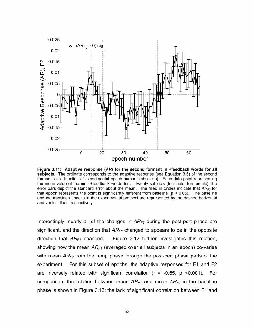
53

10 20 30 40 50 60-0.025

-0.02

-0.015

-0.01

-0.005

0

0.005

0.01

0.015

0.02

0.025

epoch number

Ada

ptiv

e R

espo

nse

(AR

), F2

(ARF2 ≠ 0) sig.

Figure 3.11: Adaptive response (AR) for the second formant in +feedback words for all subjects. The ordinate corresponds to the adaptive response (see Equation 3.6) of the second formant, as a function of experimental epoch number (abscissa). Each data point representing the mean value of the nine +feedback words for all twenty subjects (ten male, ten female); the error bars depict the standard error about the mean. The filled in circles indicate that ARF2 for that epoch represents the point is significantly different from baseline (p < 0.05). The baseline and the transition epochs in the experimental protocol are represented by the dashed horizontal and vertical lines, respectively.

Interestingly, nearly all of the changes in ARF2 during the post-pert phase are

significant, and the direction that ARF2 changed to appears to be in the opposite

direction that ARF1 changed. Figure 3.12 further investigates this relation,

showing how the mean ARF1 (averaged over all subjects in an epoch) co-varies

with mean ARF2 from the ramp phase through the post-pert phase parts of the

experiment. For this subset of epochs, the adaptive responses for F1 and F2

are inversely related with significant correlation (r = -0.65, p <0.001). For

comparison, the relation between mean ARF1 and mean ARF2 in the baseline

phase is shown in Figure 3.13; the lack of significant correlation between F1 and

54

F2 in the baseline suggests that the significant relation between changes in the

two formants results in response to the SA protocol. It should be noted that more

points were used in the correlation in Figure 3.12 than in Figure 3.13 (50 points

versus 15 points); the fewer points used in the correlation in Figure 3.13 could

partly account for the lack of significance.

As discussed in Section 3.2.3, this inverse relation may be the result of the

physiological constraints of the vocal tract. On the other hand, it may also result

from constraints on how auditory dimensions for vowels are represented (such as

in Miller ratio dimensions). It is important to note that the variability within the

second formant is small (+/-0.015 pert, which would correspond to roughly +/- 15-

30 Hz for F2); thus, even if the F2 alterations were significant, they were still

minor contributing factors in the overall adaptation. (Appendix D addresses the

issue of whether or not the changes in F2 production result from the perturbation

algorithm introducing an unintended shift in F2).

0 0.02 0.04 0.06 0.08 0.1 0.12 0.14-0.02

-0.015

-0.01

-0.005

0

0.005

0.01

0.015

0.02

mean (ARF1)epoch

mea

n (A

RF2

) epoc

h

r2 = 0.61, p < 0.001

Figure 3.12: Mean adaptive response in F2 (ARF2) as a function of mean adaptive response in F1 (ARF1), for ramp phase through post-pert epochs. The ordinate corresponds to the mean adaptive response in F2 over that epoch. The abscissa is the corresponding measure in F1. The line indicates the best regression fit, with corresponding statistics (r2 and p value) shown in the legend.

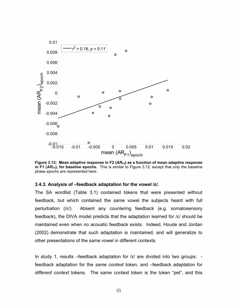
55

-0.015 -0.01 -0.005 0 0.005 0.01 0.015 0.02-0.01

-0.008

-0.006

-0.004

-0.002

0

0.002

0.004

0.006

0.008

0.01

mean (ARF1)epoch

mea

n (A

RF2

) epoc

h

r2 = 0.18, p = 0.11

Figure 3.13: Mean adaptive response in F2 (ARF2) as a function of mean adaptive response in F1 (ARF1), for baseline epochs. This is similar to Figure 3.12, except that only the baseline phase epochs are represented here.

3.4.3. Analysis of –feedback adaptation for the vowel /ε/. The SA wordlist (Table 3.1) contained tokens that were presented without

feedback, but which contained the same vowel the subjects heard with full

perturbation (/ε/). Absent any countering feedback (e.g. somatosensory

feedback), the DIVA model predicts that the adaptation learned for /ε/ should be

maintained even when no acoustic feedback exists. Indeed, Houde and Jordan

(2002) demonstrate that such adaptation is maintained, and will generalize to

other presentations of the same vowel in different contexts.

In study 1, results –feedback adaptation for /ε/ are divided into two groups: -

feedback adaptation for the same context token, and –feedback adaptation for

different context tokens. The same context token is the token “pet”, and this

56

refers to the fact that this token is also contained in the +feedback wordlist. The

different context tokens are the tokens “get” and “peg”; these tokens were not

present in the + feedback wordlist. These results are summarized in Figure 3.14

(same context) and Figure 3.15 (different context), and are depicted in a similar

manner to the F1 analysis in 3.4.2.

10 20 30 40 50 60

-0.04

-0.02

0

0.02

0.04

0.06

0.08

0.1

0.12

epoch number

Ada

ptiv

e R

espo

nse

(AR

)

F1 > 0

Figure 3.14: Adaptive response (AR) for the first formant of the –feedback token “pet” (the same context token) for all subjects exposed to 0.7 pert in F1. Same context token refers to the fact that “pet” is found in the +feedback wordlist and the –feedback wordlist. Each data point is the mean value of twenty tokens: the one –feedback token “pet” for each of the twenty subjects (ten male, ten female); the error bars depict the standard error about the mean. Refer to Figure 3.10 for further details.

Figure 3.14 indicates that the adaptation learned from the +feedback tokens does

indeed transfer to the –feedback tokens with the same vowel, same context

condition. The ARI for the –feedback “pet” tokens is significantly increased (p <

0.001) from baseline with a value of 0.0579 +/- 0.0055 (refer Table 3.2). This

ARI value was less (by almost half) of the ARI reported F1 in the +feedback

tokens: 0.0993 +/- 0.0016 (refer to Section 3.4.2). For better comparison, the

57

ARI of just the +feedback “pet” tokens was also calculated, and determined to be

0.0984 +/- 0.0044 (also significant with p <0.001)—still greater than the ARI of

the –feedback “pet” token (refer Table 3.2). The result of lower adaptation in the

–feedback tokens confirms a result seen in Houde and Jordan (2002), and is

expected if the subject can rely on other sources of feedback that the acoustic

perturbation does not immediately influence, such as somatosensory feedback (refer to Section 2.2).

Figure 3.15 shows that the adaptation generalizes to –feedback tokens of the

vowel /ε/, even when that vowel is contained in a different context from those

tokens which received perturbed feedback. The combined ARI value found for

the “get” and “peg” tokens (different context) is 0.0669 +/- 0.0041 (refer Table

3.2). While this value is less than the ARI of +feedback /ε/ tokens (confirming the

result found above), it is slightly higher than the ARI found for the –feedback “pet”

token (same context). However, paired t-test analysis of AR scores during the

full-pert phase was performed between the same context scores and the different

context scores, and showed that the two groups of –feedback tokens did not

differ significantly (p > 0.05).

58

10 20 30 40 50 60

-0.04

-0.02

0

0.02

0.04

0.06

0.08

0.1

0.12

epoch number

Adap

tive

Res

pons

e (A

R)

F1 > 0

Figure 3.15: Adaptive response (AR) for the first formant of the –feedback token “get” and “peg” combined (the different context tokens) for all subjects exposed to 0.7 pert in F1. Different context token refers to the fact that “peg” and “get” are found only in the –feedback wordlist, though they do contain the vowel /ε/, which subjects did hear perturbed in the +feedback tokens . Each data point is the mean value for all subjects for the two –feedback token “peg” and “get”; error bars depict the standard error about the mean. Refer to Figure 3.10 for further details.

The adaptive response index results from Sections 3.4.2 and 3.4.3 are

summarized in Table 3.2. For comparison to previous work, comparable

measures to the + feedback (F1), -feedback w/ same context, and – feedback w/

different context conditions were derived from the figures contained in Houde and

Jordan (1998) by taking the mean across subjects for the compensation,

adaptation, and generalization values reported. As mentioned previously the

type of perturbation and thus the metric used to measure response in Houde and

Jordan differ from this study. However, this table is informative because both

studies indicate the relative order of responses as the following: +feedback >

different context –feedback > same context –feedback.

59

ARI std. dev.Houde & Jordan response (est)

+feedback, F1 0.0993 +/-0.0016 0.55+feedback, F2 -0.0062 +/-0.0041 *

(below are for F1 only)

+feedback, same context (pet) 0.0984 +/-0.0044 n/a

-feedback, same context (pet) 0.0579 +/-0.0055 0.32

-feedback, different context (peg and get) 0.0669 +/-0.0041 0.43

Table 3.2: Summary of adaptive response index (ARI) calculated in study 1. ARI calculated according to Equation 3.5. This table summarizes all mean ARI values (calculated over the full-pert phase) reported in Section 3.4. The right column displays results derived from figures found in Houde and Jordan (1998). While their results use a different metric than in study 1, the relative orders of the measures are informative.

3.4.4. Analysis of generalized adaptation for multiple vowels. As indicated in the SA protocol wordlist (Table 3.1), several –feedback tokens

contained different vowels from the one subjects received with acoustically

perturbed feedback (/ε/). These tokens were included in the protocol to establish

the degree to which adaptation can generalize to unperturbed vowels. Figure

3.16 - Figure 3.19 summarizes the amount of adaptation found in the following

vowels: /I/ (“pit”), /i/ (“pete”), /æ/ (“pat”), /A/ (“pot”), /Λ/ (“put”), and /o/ (“pote”).

The –feedback token /ε/ is also displayed for comparison. In these figures,

subjects were subdivided into four groups (five subjects each), based on gender

and pert level used in the SA protocol (0.7 pert or 1.3 pert). For each vowel, the

mean F1 and F2 (in mel scale) are shown for the full baseline (epochs 1-15,

labeled as 1), full pert (epochs 21-45, labeled as 2) and post-pert (epochs 46-65,

labeled as 3) phases. For convenience, the arrow on each figure shows the

direction of the acoustic perturbation. (Note that data presented are separated

on the basis of gender because non-normalized formant frequencies are used,

and male speakers tend to have lower formants than female speakers.)

Overall, the adaptation generalized to other vowels. This is observed in Figure

3.16 (females) and Figure 3.17 (males) by the shifting of the max-pert phase (2)

60

to the right (increased F1) of the baseline phase (1) when the acoustic

perturbation shifted F1 down. Similarly, Figure 3.18 (females) and Figure 3.19

(males) show that an upwards F1 acoustic perturbation is accompanied by a shift

of the full-pert phase (2) to the left (i.e. a decrease) of the baseline phase (1). On

a mel scale, the adaptation seen in the vowels /I/, /æ/, and /A/ was consistently

as large, or even larger (see /æ/ and /A/ Figure 3.18 and Figure 3.19).

Exceptions to the generalization of vowel adaptation have been observed. For

the vowel /i/, changes in F1 were either small in the female subjects or

insignificant—that is, not outside the standard error—in the male subjects. For

the vowel /o/, significant adaptation was observed in all conditions except the 1.3

pert male subjects (Figure 3.19). In this same set of subjects, the vowel /Λ/ is

observed to change in the same direction as the adaptation, as opposed to a

compensatory direction (Figure 3.19). Finally, while the adaptation was specific

to F1 in most cases, the 0.7 pert female subjects showed changes in F2 (outside

the standard error) for the vowels /Λ/, /o/, and /A/ (Figure 3.16).

The degree to which subjects returned to the baseline vowel positions during the

post-pert phase (3) was variable, though most vowels that showed an adaptive

response also showed at least partial return to baseline. Close to full return to

baseline was exhibited in many of the post-pert phase (3) vowels—specifically /I/,

/ε/, /æ/ and /A/—from the subjects shown in Figure 3.19 (1.3 pert males subjects).

On the other hand, little return to baseline was evident in several instances: /U/

for 0.7 pert female subjects (Figure 3.16), /æ/ for 0.7 males subjects (Figure

3.17), and the /o/ and /A/ vowels of 1.3 female subjects (Figure 3.18). The

remaining vowels returned to baseline to an intermediate degree.

61

400 500 600 700 800 900 10001100

1200

1300

1400

1500

1600

1700

1800

i

I

ε

Q

Λ

o

A

←

1 23

12

3

1

2

3

1

2

3

1 23

1

23

123

mean F1 (mels)

mea

n F2

(mel

s)1 baseline2 full-pert3 post-pert

Figure 3.16: Shift in F1/F2 vowel space for all vowels of the -feedback tokens, 0.7 pert female subjects. Shown here are the formant values for the vowels presented without feedback in the "pXt" context. The light colored crosses with the 1 label correspond to the values in the baseline phase (epochs 1-15); the medium colored crosses with the 2 label correspond to the values in the full perturbation phase (epochs (21-45); the dark colored crosses with the 3 label correspond to the mean values in the post perturbation phase (epochs 46-65). The abscissa shows F1 in mels, averaged among five subjects and all the trials within a given phase. The ordinate shows F2 in mels. The vertical and horizontal lines represent standard error about the mean of the formants. The arrow indicates the direction of the perturbation the subjects were exposed to (down shift in F1).

62

400 450 500 550 600 650 700 750 800900

1000

1100

1200

1300

1400

1500

1600

i

I

ε

Q

Λ

o

A

←

123

1 23

1 23

1 23

123

1 23

1 23

mean F1 (mels)

mea

n F2

(mel

s)

1 baseline2 full-pert3 post-pert

Figure 3.17: Shift in F1/F2 vowel space for all vowels of the -feedback tokens, 0.7 pert male subjects. See Figure 3.16 for figure explanation.

450 500 550 600 650 700 750 800 850 9001100

1200

1300

1400

1500

1600

1700

1800

i

I

εQ

Λ

o

A

→

12 3

12

3

1

23

123

123

12 3

12 3

mean F1 (mels)

mea

n F2

(mel

s)

1 baseline2 full-pert3 post-pert

Figure 3.18: Shift in F1/F2 vowel space for all vowels of the -feedback tokens, 1.3 pert female subjects. See Figure 3.16 for figure explanation.

63

400 450 500 550 600 650 700 7501000

1100

1200

1300

1400

1500

1600

1700

i

I

ε

Q

Λ

oA

→

12 3

12

3

12 3

123

123

123

1

23

mean F1 (mels)

mea

n F2

(mel

s)1 baseline2 full-pert3 post-pert

Figure 3.19: Shift in F1/F2 vowel space for all vowels of the -feedback tokens, 1.3 pert male subjects. See Figure 3.16 for figure explanation.

The generalization of adaptation to other vowels suggests that the subjects are

not learning to modify a vocal tract configuration that is specific to just the vowel

that was perturbed in the SA feedback—the vowel /ε/. Rather, subjects appear

to have learned to modify the vocal tract in a way that the adapted response can

be applied globally to other vowels. Specifically, changes in the first formant can

be accomplished by simply controlling the height of the jaw during vowel

production (Stevens, 1998). Moreover, generalization is an advantageous

property to have in the speech motor planning system, since people do not often

repeat the same words when normally speaking. Applying adaptation learned for

one specific context more globally is a behavior that enhances an individual’s

ability to more quickly react to different acoustic feedback conditions, and

maintain intelligibility of the communicated utterances in spite of the altered

feedback.

64

3.4.5. Analysis of the contribution of F0 to adaptation. Figure 3.20 shows F0 as a function of epoch number, plotted in a similar manner

as F1 and F2 were in Figure 3.8: normalized to the mean of the baseline

epochs. Figure 3.20 shows that both types of subjects—those exposed to the

0.7 pert shift and those exposed to the 1.3 pert shift—showed a general trend of

F0 increasing throughout the SA protocol. Interestingly, subjects exposed to the

0.7 pert shift increased in F0 to a lesser degree (dashed line) than subjects

exposed to the 1.3 pert shift (solid line). When factoring out the portion of F0

increase that was common to both pert groups, another trend in F0 was found:

subjects tended to produce a shift in F0 that was in the opposite direction of the

F1 shift they produced.

This result is not an unsurprising, considering that investigators who conducted a

comparable experiment by perturbing F0 in the acoustic feedback (Jones and

Munhall, 2000) found a similar trend. They also found F0 generally increased

for subjects, regardless of whether they were exposed to the shift-up, shift-down

or control protocols. At the same time, Jones and Munhall also found that

subjects exposed to the shift down protocol increased in F0 to a greater degree

in F0 than the control, while subjects exposed to the shift up protocol increased

in F0 to a lesser degree than the control. That is, when the common increase in

F0 was factored out, subjects in the Jones and Munhall experiment produced a

shift in F0 that was opposite of acoustic F0 perturbation.

65

10 20 30 40 50 600.97

0.98

0.99

1

1.01

1.02

1.03

1.04

1.05

1.06

1.07

epoch

norm

aliz

ed F

00.7 pert1.3 pert

Figure 3.20: F0 normalized to the mean of the baseline epochs (1-15), as a function of epoch number. The solid line represents the mean of the subjects exposed to the 0.7 pert shift, while the dashed line represents the mean of the subjects exposed to the 1.3 pert shift. The vertical lines indicate the transitions in pert level.

In the current acoustic F1 perturbation SA experiment, the additional change in

F0 (factoring out the upward trend common to both conditions) seems to be in

the opposite direction of the compensatory shift in F1 the subjects produced.

Figure 3.21 demonstrates this relation, showing the F0 difference versus F1

difference, with both quantities normalized to the mean of the baseline epochs.

F0 difference—defined here as the difference between the subject’s normalized

F0 and the mean normalized F0 for all subjects in the given epoch—is used to

factor out the rising F0 that occurs for all subjects in the experimental session.

(For consistency, the F1 difference—defined in the same manner as F0

difference—is used in the ordinate.) This figure demonstrates that a significant

(r2 = 0.55, p < 0.001) inverse relation exists between F1 and F0 production,

similar to the relation between F1 and F2 (see 3.4.2). When considered

66

separately, the 0.7 pert subjects and 1.3 subjects both showed significant—

p<0.01 in each case—negative correlation as well. The inverse relation between

F1 and F0 may indicate that subjects perceive, and thus compensate for, a

quantity—such the Miller ratio (Miller, 1989)—that incorporates F0 as well as F1.

-0.03 -0.02 -0.01 0 0.01 0.02 0.03-0.2

-0.15

-0.1

-0.05

0

0.05

0.1

0.15

[normF0 difference]epoch

[nor

mF1

diff

eren

ce] ep

och

0.7 pert1.3 pertrall

r0.7 pert

r1.3 pert

Figure 3.21: Correlation between normalized F0 difference and the normalized F1 difference, over the full pert epochs. The abscissa corresponds to the difference between a subject’s normalized F0 and the mean of all subjects’ normalized F0, both calculated for a given epoch. The ordinate is the normalized F1 difference, calculated the same way as the F0 difference. The open circles correspond to data from 0.7 pert subjects; the asterisks correspond to data from 1.3 pert subjects. The lines indicate the best regression fit, all of which have significant correlation (p < 0.001). The dashed-dotted line corresponds to the correlation of the 0.7 pert data, the dashed line corresponds to the 1.3 pert data, and the solid line corresponds to all data. Only epochs 21 to 65 (full-pert and post-pert epochs) from nineteen subjects are shown; one subject was excluded from this analysis (see text).

3.4.6. Analysis of within token adaptation. Data from study 1 were reanalyzed to investigate possible evidence of “within

token” adaptation (refer to Section 3.2.5). In this analysis, each +feedback token

was divided into ten equal-length sections based on the duration of the token:

67

that is, section 1 represents the first ten percent of the token, section 2

represents the second ten percent of the token, and so on, up to section 10,

representing the last ten percent of the token (see Figure 3.22.) Formants were

extracted from each segment using the same LPC analysis tool described in

3.3.4, with the major difference being the segment length to which the formant

extraction was applied. To allow investigation of how each segment changes

relative to epoch number, these sectional F1 values were normalized by the

mean baseline F1 value within the corresponding section, and segmental

adaptive response values were then determined for +feedback tokens of all

subjects (using Equation 3.5). The segments investigated in the following

analysis are the front segment (defined here as the second and third sections)

and the end segment (defined here as the eighth and ninth sections); the first

and tenth sections were excluded from analysis to avoid possibly confounding

co-articulatory influence from the neighboring stop consonants.

time

RM

S

Figure 3.22: Example of time segmentation of tokens for within-vowel adaptation. For within-token analysis, tokens are divided into ten sections of equal duration (vertical lines), from which F1 values are extracted. The darker segments indicate the front and end segments of the vowel which were compared for evidence of within-vowel adaptation. The abscissa is in units of milliseconds.

The adaptive response for the front (solid line) and end (dashed line) vowel

segments throughout the SA experiment are shown in Figure 3.23. In this figure,

68

it is evident that the front and end segments generally change at the same rate

during the experiment, even near the phase transitions (i.e. the beginning of the

ramp phase and the beginning of the post-pert phase). Paired, two-tail t-test

analysis between front and end segments performed on an epoch-by-epoch

basis showed that the two segments differed significantly only at one epoch

(epoch 61).

The lack of any significant adaptative response differences between the front and

the end of the vowel may likely result from the design of this protocol. That is,

within-vowel differences may only be evident on a time-scale that is shorter than

an epoch. However, because each epoch contains tokens of different phonetic

contexts, it is difficult to separate within-epoch differences that are due to a lag in

compensatory response (as hypothesized in 3.2.5) from those that are due to

contextual differences. It should be noted that signficant within-vowel adaptation

effects has been noted in another SA experiment that used the same

perturbation algorithmn used in this thesis (Tourville et al., 2005).

0 10 20 30 40 50 60

-0.04

-0.02

0

0.02

0.04

0.06

0.08

0.1

0.12

epoch number

sect

iona

l ada

ptiv

e re

spon

se

frontend

Figure 3.23: Segmental adaptive response for the front and end vowel segments during the entire SA protocol. The front segment of the vowel is shown in solid line; the end segment is shown in dashed line. The vertical lines indicate transitions in pert level: the leftmost line indicates the start of the ramp phase, the middle line indicates the start of the full-pert phase, and the rightmost line indicates the start of the post-pert phase.

69

3.5. Study 1 summary. Results from this study indicate that, in response to perturbations of the first

formant in the acoustic feedback of vowel productions, subjects compensate by

shifting this formant in a direction opposite to the perturbation. This adaptation

persisted even when subjects received feedback blocked by masking noise.

Additionally, even though only tokens containing the vowel /ε/ received perturbed

feedback, the adapted shift in F1 generalized to tokens containing other vowels

as well. Subjects also demonstrated that they maintained this adaptation for a

brief period after the perturbation was removed. These results are consistent

with findings in other sensorimotor adaptation experiments in speech (Houde

and Jordan, 1998; Houde and Jordan, 2002; Max et al., 2003).

This study here also suggests findings previously unreported for speech

sensorimotor adaptation. That is, while the adaptive response was expressed

mainly in compensation of the formant that was perturbed (F1), subjects also

demonstrated that the second formant (F2) and even the fundamental frequency

(F0) changed in a significant way due to the F1 perturbation. However, it should

be noted that the analysis was not able to detect within-vowel differences in

adaptation.

The analysis in this chapter focused largely on adaptation properties revealed by

treating the entire subject set as a whole. The following study will investigate

how degree of adaptation varies from one subject to another, focusing largely on

the relation between perceptual acuity and adaptation.

70

Chapter 4. Cross-correlation comparison between vowel discrimination and SA (study 2).

4.1. Background and specific aims of the perceptual acuity experiment.

The purpose of study 2 is to account for some of the individual variations in the

ability of subjects to adapt to the acoustic speech perturbation. Specifically, this

study focuses on the relation between individual acuity—i.e. ability to distinguish

fine details—in the perception of the perturbation and the ability to adapt to it.

4.1.1. Relation between vowel discrimination and adaptation.

Recent work has tested a prediction of the DIVA model on the relation between

speech perception and production. A central concept to this relation is the goal

region—defined here as a bounded set of sensory expectations for the correct

production of a given phoneme, and illustrated in Figure 4.1. Vowels with

auditory dimensions (F1, F2) that fall within the goal region are judged as correct

productions of that vowel, while vowels with (F1, F2) falling outside the goal

region are judged as incorrect productions. In line with the feedback control

mechanism discussed in Section 2.3, speakers that judge their own vowel as

incorrectly produced are expected to correct for this error. Thus, the size of the

sensory goal region—a perceptual phenomenon based on the discrimination of

speech acoustics—determines the role of feedback error correction in speech

production. As discussed in Section 2.3, the predicted relation—greater

discrimination of speech acoustics occurring with greater contrast in speech

production—has been observed in cross-subject correlations between speech

production and discrimination (Newman, 2003; Perkell et al., 2004b; Perkell et

al., 2004a); other evidence for sensory goal regions is discussed in Section 5.1.2.

71

F2

F1

/E/

Perturbation

“correct” vowel

F2

F1

/ε/

“incorrect” vowel

Figure 4.1: The auditory goal region. The “auditory” goal region (circle) for a phoneme (here, the vowel /ε/) is shown in a two-dimensional (F1,F2) space. Vowels that are perceived to fall within the goal region are judged as “correct” vowel productions, while vowels that are perceived to fall outside the goal region are judged as “incorrect” vowel productions. One consequence of the prediction relating perception and production is that

subjects with more acute speech perception should be able to better adapt their

speech to perceived auditory errors (such as those that were introduced by the

SA protocol). Figure 4.2 illustrates the auditory goal regions for the vowel /ε/ for

two hypothetical subject types, and relates goal region size to extent of

adaptation (straight lines pointing to the left) due to the perturbation (dotted line

pointing to the right). Subjects that are not able to discriminate differences in

the vowel acoustics well (low acuity speakers) are expected to have larger

auditory goal regions representing their vowels; on the other hand, subjects that

can discriminate fine changes in the vowel acoustics (high acuity speakers) are

expected to have smaller auditory goal regions.

In the Figure 4.2 example, both hypothetical subjects are exposed to the same

size auditory perturbation, which shifts F1 up. In response to the auditory

perturbation, the subject with the smaller auditory goal region will have to adapt

to a greater extent (solid line) to cause the production of that vowel to be

perceptibly acceptable—that is, within the boundaries of the auditory goal

regions—especially when compared to the adaptive response (dashed line) of

72

the subject with a larger auditory goal region. Since the size of the auditory goal

regions of speech is dependent on auditory acuity, it follows that subjects that

demonstrate better perceptual acuity of speech should show greater SA

response. This relationship can be investigated by performing a vowel

discrimination experiment on subjects from study 1, and correlating the results of

these two studies across subjects.

Figure 4.2: Proposed relation between auditory goal region size and adaptive response. The two circles represent the auditory goal regions of the vowel /ε/ for two hypothetical subjects: a high acuity subject (solid line circle), who has a smaller goal region size; and a low acuity subject (dashed line circle), who has a larger goal region. For the same degree of perturbation (black dotted line to the right), the subject with smaller goal region will demonstrate greater adaptive response (solid line to the left), than when compared to the adaptive response of the subject with the larger goal region (dashed line to the left). Adapted with permission from Perkell, et al (unpublished).

This series of experiments was designed to study the relation between an

individual’s ability to adapt to an acoustic perturbation in speech and his/her

perceptual acuity of that perturbation. Subjects that participated in study 1 on

this project were recalled to participate in a battery of speech perception

experiments. Results from these experiments were then correlated with

measurements of adaptive response obtained in the experiments described in

Chapter 3.

F2

F1

/E/

Perturbation

LOHI

Compensatory responses

F2

F1

/E/

Perturbation

LOHI

Compensatory responses

73

4.1.2. Relation between vowel spacing and adaptation.

Since the SA experiment included baseline (epochs 1-15) tokens of the vowels

/æ/, /ε/, and /I/ (“pat”, “pet”, and “pit” –feedback tokens, respectively), the

relationship between baseline vowel separation in F1 and adaptive response can

also be measured. While this relationship was not taken into account during the

design of the SA and perceptual acuity experiments, it is reasonable to expect it

exists. Two alternative hypotheses relating vowel spacing and adaptation are

considered here.

When a subject hears the perturbed vowel during the full-pert epochs, the subject

may compensate by an amount that is proportional to the separation between the

perceived (i.e. perturbed) vowel and the target vowel (i.e. unperturbed) vowel.

Consider a subject trained on the 0.7 pert SA protocol, which shifts the sound of

the vowel /ε/ to sound like the vowel /I/ (i.e. shift-down in F1). If that subject’s

baseline /ε/ and /I/ vowels are close together in F1, he may not perceive the need

to increase the perturbed F1 greatly to shift his perception of the vowel from an

/I/ to an /ε/. However, if the subject’s baseline F1 of these vowels are separated

widely, he or she may attempt a greater correction to shift the perceived vowel

back to / ε/. This proposed relation is illustrated in Figure 4.3.8

An alternative hypothesis suggests that vowel spacing and adaptation are related

in the opposite manner: subjects who have vowels spaced further apart in the

first formant dimension will adapt less than those with closely spaced vowels.

This idea arises from the assumption that, for a fixed perturbation, subjects with

closely spaced vowels are more likely to perceive the perturbation than subjects

with vowels spaced further apart. This increased likelihood in perception of the

perturbation would then lead to a larger adaptive response, in the alternative

hypothesis. Considering these competing hypotheses about the relation

between produced vowel spacing and adaptation, the following study addresses 8 This hypothesis implies that subjects with larger vowel spacing will make larger corrections during the perturbation phase, thus leading to larger adaptation than subjects with smaller vowel spacing (who would make smaller corrections).

74

how perceptual acuity, produced vowel spacing and adaptation relate to one

another.

/ε/

F1

F2

/I/,close

/I/,far

perturbation

Figure 4.3: Proposed relation between vowel spacing and adaptation. Representation of auditory goal regions of F1 for two hypothetical subjects shown here: one whose baseline F1 for the vowel /I/ is close to the vowel /ε/, and one whose baseline F1 for the vowel /I/ is far from the vowel /ε/. Here, the auditory goal region for the vowel /ε/ is the same in both hypothetical subjects. Each subject experiences the same size perturbation in F1 of the /ε/ vowel (dotted line). Assuming both subjects perceive they have spoken the vowel /I/ during the perturbation, one likely correction each subject may undertake (at least initially) is to increase F1 by an amount proportional to the spacing between /I/ (the incorrect vowel) and /ε/ (the correct vowel). Thus, the subject with /I/ that is close to/ε/ will make a smaller correction (dashed line) than the subject with /I/ that is far from /ε/ (solid line).

4.2. Methodology of study 2: the perceptual acuity experiment.

The battery of perceptual acuity experiments was broken down into four steps:

speech recording, an adaptive staircase discrimination task, a second

discrimination task, and a goodness rating task. From this battery, the just

noticeable difference (jnd) was determined from the discrimination task, and

other perceptual measures were determined from the goodness rating results.

The use of a two-stage protocol for measuring jnd was based on work from other

researchers (Guenther et al., 1999b; Guenther et al., 2004) showing that tihs

method results in a more precise measure of jnd.

75

Note that subjects with greater auditory acuity should be able to resolve finer

differences; thus, subjects with greater acuity with respect to the perturbation

should have smaller jnd values.

4.2.1. Participating subjects.

The same set of subjects that were used in the SA study also participated in this

experiment. Seven out of the twenty subjects were no longer available at the

time the second study was conducted, so the results from the acuity experiment

were based on thirteen subjects.

4.2.2. Recording of the subject’s speech.

The speech recordings were conducted in a sound attenuating room using a

head-mounted piezo-electric microphone (Audio-Technica, model AT803B)

placed at a fixed distance of 20 cm from the speaker’s lips. Elicited utterances

were presented on a monitor. The monitor also displayed cues that induced the

subject to speak at a target loudness (85 +/- 2 dB SPL) and word duration (300

msecs)9. Subjects were allowed to practice to achieve these targets. Subjects

were then instructed to speak ten tokens each of the following words: “bet”, “bit”

and “bat”. The F1 frequency for each “bet” token was measured, and the “bet”

token with the median F1 value was selected as the base token.

The following perceptual acuity tests were carried out in the same sound

attenuating room that the recordings were made in, though not necessarily on the

same day. Subjects heard stimuli over closed back headphones (Sennheiser

EH2200), played on a computer controlled by Matlab script.

9 The displayed loudness cue displayed the SPL as a bar with the ideal range marked off. The duration cue consisted of a change in display background color from white to gray after 300msec from the onset of voicing. These are the same visual cues used to control loudness and word duration in study 1.

76

4.2.3. Staircase protocol to estimate jnd.

The purpose of this staircase protocol is to obtain an approximate estimate jnd.

The second stage of the discrimination task can yield a better estimate of the

subject’s jnd, but only over a limited range of pert values. By using the estimate

from this first stage to determine the range of tokens for the second stage, it is

more likely that the second stage of the discrimination task will operate in the

subject’s most sensitive range.

Three milestone synthetic stimuli were generated from the base token, spaced at

0.85 pert, 1.0 pert (i.e. identical to the base token) and 1.15 pert apart. Around

each milestone, an adaptive, 1-up, 2-down staircase protocol was run to estimate

the jnd for that milestone. In this procedure, pairs of tokens that were either the

same or different from each other were presented to the subject with equal

probability. The members of the same pairs both consisted of the milestone,

while the different pairs consisted of tokens straddling the milestone equally

spaced in pert. Whenever the subject responded incorrectly to either the same

or different pairs, the distance between the different pairs increased. Whenever

the subject responded correctly to two presentations of a given different pair, the

distance between the different pairs decreased. The separation was unchanged

when the subject responds correctly to a same pair presentation. The order of

the three staircase protocols was randomized for each subject.

The stimuli pairs were separated initially by 0.30 pert from each other. The first

four changes in separation were 0.04 pert, followed by changes in pert

separation of 0.02 pert after that. Once the tokens got to within 0.10 pert from

each other, the separation was only changed by 0.01 pert. After eight reversals

(changes in direction of the staircase), the protocol terminated, and the jndest was

calculated as the median value of the last four reversals on the staircase.

Two subjects participating in this experiment had jndest that were higher than the

initial value set at the beginning of the staircase protocol. (That is, the staircase

77

“climbed” rather than “descended”.) When this occurred, a new continuum of

perturbed tokens was generated from new recordings of the subject’s speech,

and the entire speech acuity experiment was re-run.

0 10 20 30 40 50 600

0.05

0.1

0.15

0.2

0.25

0.3

presentation number

pert

sepa

ratio

n

first four steps = 0.04 pert

steps = 0.01 pert when sep. < 0.1

following steps = 0.02 pert

Figure 4.4: Example an adaptive rocedure used to estimate jnd. The abscissa shows the presentation number of the given pair, and the ordinate depicts the separation of the different pairs in pert. The text within the figure gives conditions for changes in step size. The staircase terminated after eight reversals of the staircase. Refer to Section 4.2.3 for a more detailed explanation of the procedure.

4.2.4. A more precise same-different protocol.

Three blocks (one for each milestone) of a more precise same-different protocol

were then run on each subject. In this protocol, presented tokens were either the

same (both = milestones) or different (straddling the milestone, refer to Figure

4.5). The different pairs were spaced by the following multiples of the jndest: +/-

0.25, +/-0.5, +/-0.75, +/-1.0 and +/-1.4. The +multiple of the jndest pair was

always presented with the corresponding –multiple for a different pair

presentation, though the order of which token was first presented was

78

randomized. Each unique pair (the one same and five different pairs) was

presented to the subject 50 times, for a total of 300 presentations per block.

Subjects were given feedback as to the correct response to the pair just

presented. Both the order of presentations within each block, and the order in

which the blocks occurred, were randomized.

-1.4 -1 -0.75 -0.5 -0.25 0 0.25 0.5 0.75 1 1.4token pairs (multiples of jndest)

Figure 4.5: Token pairs used within the more precise same-different protocol. The abscissa depicts the separation of the stimuli in the pairs of tokens used within a given block of the more precise same-different protocol, measured as a multiple of the jndest obtained from the staircase procedure. The milestone (also the same pair) is represented by the 0 token. Branches join the tokens that are paired together in a given different presentation. Note that the members of each pair are equally spaced from the milestone (when measured in pert), thus the different pairs “straddle” the milestone.

4.2.5. Goodness rating task.

A continuum of 41 tokens, evenly spaced in pert and ranging from 0.7 to 1.3 pert,

was then generated from the subject’s base token. The subject performed two

test blocks—one with 0.7 to 1.0 pert tokens and the other with 1.0 to 1.3 pert

tokens—of goodness rating tasks, in which he or she was instructed to rate the

79

token on a scale from 0 to 7, with 7 as the best example of the token /ε/.10 The

test blocks contained tokens ranging from either 0.7 to 1.0 pert, or 1.0 to 1.3 pert.

Subjects were allowed to replay the token, and were given a practice block

(which went through the entire continuum in random order) before the test block.

In the test blocks, the continuum of 21 tokens was presented in five repetitions,

and the tokens were randomized within each repetition. These goodness rating

scores were ultimately used to determine vowel category width (see Section

4.3.5); in this perceptual acuity measure, smaller category widths are presumed

to reflect higher vowel discrimination.

4.3. Analysis and correlation results.

4.3.1. Analysis of d’ scores.

The d’ score for each pair was calculated using the standard signal detection

theory formula (Macmillan and Creelman, 2005):

Equation 4.1: d’ = z(H) – z(F)

where z is the normal inverse function, H is the hit rate (responds

“different”|different) and F is the false alarm rate (responds “different”|same).

Because z score values of 1 and 0 are undefined, all rates are calculated out of

50.5 (rather than 50 presentations), and rates of zero are increased to 0.5 out of

50.5.

Data consisting of d’ score as a function pair separation (in perts) were then fitted

with a sigmoid function. A sigmoid function was used in this case because this

function is monotonic and best captures the sharp rise of d’ in the sensitive

region, while also capturing ceiling and floor properties observed in the data.

10 The continuum for the goodness rating task was divided into two—rather than presenting the entire continuum in one task—to allow increased contrast between the base token and the tokens at the extreme of the continuum. In pilot studies, subjects tended to rate the base token and the extreme tokens closer together when all tokens were presented in one task.

80

Note that, in fitting the data, the origin (0 pert jnd, 0 d’score) is included as a data

point.

Some subjects had d’ vs. pert separation functions whose maximal d’ value was

less than 1.0. Consequently, the criterion for the jnd used here was the maximal

d’ value common to all subjects run on the perceptual acuity protocol, in this

case, 0.7. Thus, the jnd was defined here the pert separation corresponding to a

d’ score of 0.7, as determined by from the best fit function (refer to Figure 4.6).

0 0.02 0.04 0.06 0.08 0.1 0.12 0.14 0.160

0.5

1

1.5

2

jnd @ dprime = 0.7 intercept

d prim

e

pert separation

measured pointssigmoid fit

Figure 4.6: Example of calculating jnd more precisely from the “same-different” d’ scores. This graph portrays d’ score (ordinate) obtained for one subject under one milestone condition, as a function of pert separation of the different tokens (abscissa). The open circles correspond to measured d’; the solid curve depicts the best fitting sigmoid curve. The jnd is measured as the pert separation corresponding to a d’ score of 0.7. (dashed arrow).

4.3.2. Correlation between jnd scores and adaptation scores.

The subjects’ jnd scores were subsequently correlated with their adaptive

response indices, as shown in Figure 4.7, Figure 4.8, and Figure 4.9. The

81

milestone = “same” figure (Figure 4.7) shows the jnd values at the 0.85 pert

milestone for the 0.7 pert trained subjects (open circles) grouped with the jnd of

the 1.15 pert milestone for the 1.3 pert trained subjects (crosses). The

milestone = “center” figure (Figure 4.8) presents the jnd at the 1.0 pert

milestone for the 0.7 pert trained subjects (open circles) and the 1.3 pert trained

subjects (crosses). The milestone = “opposite” figure (Figure 4.9) presents the

jnd at the 0.85 pert milestone for the 0.7 pert trained subjects (open circles)

grouped with the jnd of the 1.15 pert milestone for the 1.3 pert trained subjects

(crosses). Each figure shows a regression line, along with r2 (amount of variation

accounted for) and p-value (significance) shown in the legend.

Figure 4.7 to Figure 4.9 all demonstrate the predicted trend: subjects with smaller

jnds tend to adapt to a greater extent. For the same and opposite milestones,

these correlations account for little of the variation, and neither is significant

(defined as p scores < 0.05). On the other hand, relation between jnd and

adaptive response for the center milestone is significant (p < 0.047); this relation

accounts for 31 percent of the variance.

The hypothesis proposed in Section 4.1.1 states that adaptation should depend

on the auditory discrimination of the speech target—the auditory goal region.

Since the target vowel for adaptation was the vowel /ε/, it follows that the center milestone jnd—measuring the perceptual discrimination of the vowel /ε/--should

correlate significantly to adaptive response. Had subjects demonstrated a

significant correlation between jnd measured on the same side milestone, this

would have indicated that adaptation is also significantly dependent on the

perception of the perturbed speech. However, Figure 4.7 seems to indicate that

this is not the case. One explanation for this outcome is that the perturbed

speech perceived by each subject was not constant during the SA protocol, since

the amount that each subject adapted—which can be seen in the variation in ARI

scores—affects the perception of the perturbed speech. Thus, it is not surprising

82

that when a constant milestone—the same milestone—was used to measure the

perception of the perturbed speech, no correlation was found with adaptation.

Further, had subjects demonstrated a significant correlation between the

opposite milestone jnd and adaptive response, this would have suggested that

the acoustics related to the subject’s produced speech during the perturbation

affected adaptation. This is a particularly unlikely outcome since subjects could

not have heard their own adapted production, given the perturbed acoustic

feedback. The lack of correlation between adaptive response and the jnds

measured at the non-center milestones reinforces the notion that it is the ability

of the subject to perceive a difference from the expected acoustics that drives

adaptation.

Finally, the statistical analysis reported here was repeated using jnd estimated

from the first-stage of the two-stage discrimination task. This analysis (refer to

Appendix E) found no significant correlation.

83

-0.05 0 0.05 0.1 0.15

0.02

0.03

0.04

0.05

0.06

0.07

milestone = same

Adaptive Response Index

jnd

(per

t)r2 = 0.135, p = 0.107

Figure 4.7: Adaptive response index is not correlated with the jnd score of the milestone in the same direction as the SA training. The 0.85 pert milestone jnd score was used for 0.7 pert trained subjects (open circles), while the 1.15 pert milestone jnd score was used for the 1.3 pert trained subjects (crosses). The abscissa shows the adaptive response index, discussed above. The ordinate shows the jnd (in pert) for the “same” milestone, as determined in the “same-different” protocol. Statistics for the regression line are shown in the legend; the p-score reported uses a two-tail t-test.

84

0 0.05 0.1 0.15

0.015

0.02

0.025

0.03

0.035

0.04

0.045

milestone = center


jnd

(per

t)

r2 = 0.312, p = 0.047

Figure 4.8: Adaptive response index is correlated with the jnd score of the center milestone. The 1.0 pert milestone jnd score was used for 0.7 pert (open circles) and 1.3 pert (crosses) trained subjects. Refer to Figure 4.7 for axis and legend details.

0 0.05 0.1 0.15

0.015

0.02

0.025

0.03

0.035

0.04

0.045

0.05

milestone = opp.


jnd

(per

t)

r2 = 0.088, p = 0.322

Figure 4.9: Adaptive response index is not correlated with the jnd score of the milestone in the opposite direction of the SA training. The 1.15 pert milestone jnd score was used for 0.7 pert trained subjects (open circles), while the 0.85 pert milestone jnd score was used for the 1.3 pert trained subjects (crosses). Refer to Figure 4.7 for axis and legend details.

85

4.3.3. Correlation between vowel F1 separation and adaptation scores.

To calculate F1 vowel separation, the following calculations were made. Note

that the F1_separation values are normalized by the baseline F1 from the word

“pet”. All F1 values were taken from the baseline phase tokens. Since the

tokens “pat” and “pit” were only presented as –feedback tokens, F1 values of

“pet” were taken from the –feedback tokens for consistency.

Equation 4.2:

median

medianmedianpetpat

median

medianmedianpitpet

FpetFpetFpat

separationF

FpetFpitFpet

separationF

1_1_1_

_1

1_1_1_

_1

−=

−=

−

−

Figure 4.10 and Figure 4.11 show the produced vowel separation as a function of

Adaptive Response Index. As with the jnd scores in the correlation studies

above, Figure 4.10 (same) grouped the F1_separationpet-pit from 0.7 pert trained

subjects with the F1_separationpat-pet from the 1.3 pert trained subjects.

Conversely, Figure 4.11 (opposite) grouped the F1_separationpet-pit from 1.3 pert

trained subjects with the F1_separationpat-pet from the 0.7 pert trained subjects.

Figure 4.10 shows that subjects with larger vowel separation (on the same side

as the perturbation) do tend to adapt to a greater extent. However, this

correlation is not large (accounting for only 15 percent of the variance), and does

not reach significance (p value = 0.082). The results shown in Figure 4.11

verifies that there is no significant relationship (p value = 0.706) between vowel

separation on the opposite side of the perturbation, and adaptation.

86

-0.05 0 0.05 0.1 0.15 0.2 0.25 0.30

0.1

0.2

0.3

0.4

0.5

0.6

0.7"Same" side vowel separation

Adaptive Response Index (ARI)

base

line

vow

el F

1 se

p., n

orm

aliz

ed

r2 = 0.157, p = 0.0820.7 pert SA1.3 pert SA

Figure 4.10: Adaptive response index is not correlated with the baseline vowel F1 separation on the same side as the perturbation. The /ε/ - /I/ separation was used for subjects run on the 0.7 pert protocol (open circles), while the /æ/ - /ε/ separation was used for subjects run on the 1.3 pert protocol (asterisks). The abscissa shows the adaptive response index. The ordinate is the value of the F1 difference between the two vowels, normalized by the median baseline F1 value for /ε/ (Equation 4.3). Statistics for the regression line are shown in the legend.

-0.05 0 0.05 0.1 0.15 0.2 0.25 0.30

0.05

0.1

0.15

0.2

0.25

0.3

0.35

0.4"Opposite" side vowel separation


base

line

vow

el F

1 se

p., n

orm

aliz

ed

r2 = 0.008, p = 0.7060.7 pert SA1.3 pert SA

Figure 4.11: Adaptive response index is not correlated with the baseline vowel F1 separation on the opposite side of the perturbation. The /æ/ - /ε/ separation was used for subjects run on the 0.7 pert protocol (open circles), while the /ε/ - /I/ separation was used for subjects run on the 1.3 pert protocol (asterisks). Refer to Figure 4.10 for axis and legend details.

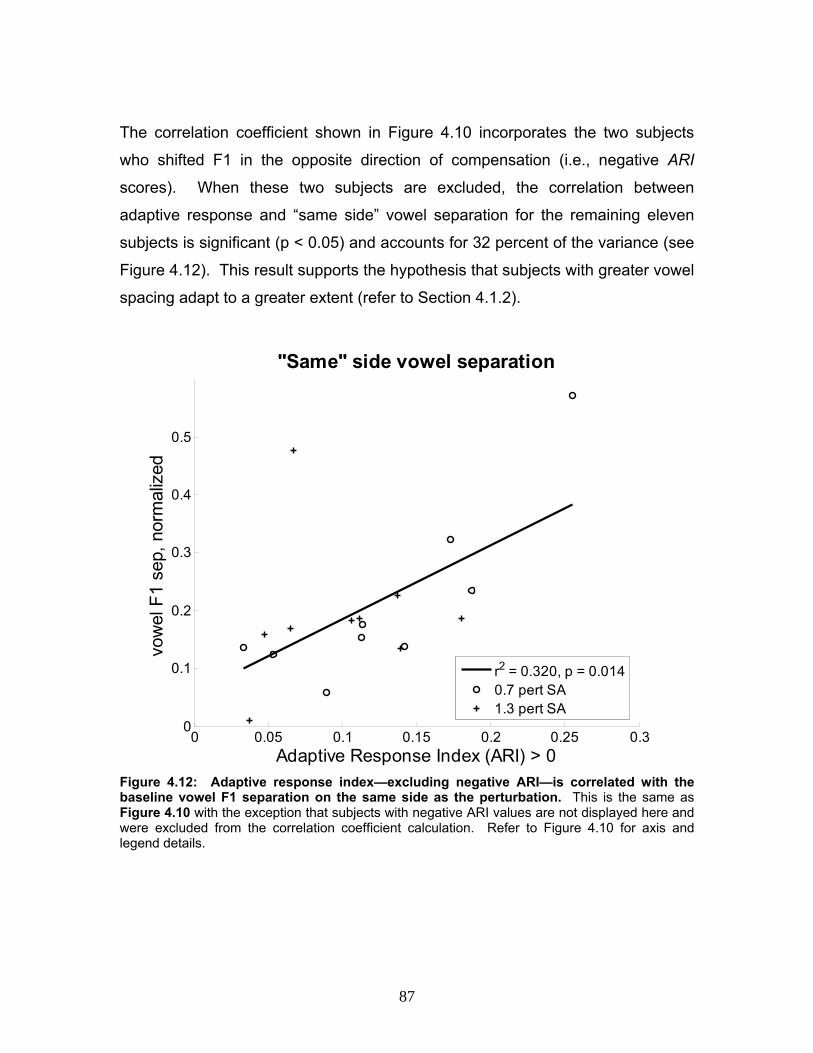
87

The correlation coefficient shown in Figure 4.10 incorporates the two subjects

who shifted F1 in the opposite direction of compensation (i.e., negative ARI

scores). When these two subjects are excluded, the correlation between

adaptive response and “same side” vowel separation for the remaining eleven

subjects is significant (p < 0.05) and accounts for 32 percent of the variance (see

Figure 4.12). This result supports the hypothesis that subjects with greater vowel

spacing adapt to a greater extent (refer to Section 4.1.2).

0 0.05 0.1 0.15 0.2 0.25 0.30

0.1

0.2

0.3

0.4

0.5

"Same" side vowel separation

Adaptive Response Index (ARI) > 0

vow

el F

1 se

p, n

orm

aliz

ed

r2 = 0.320, p = 0.0140.7 pert SA1.3 pert SA

Figure 4.12: Adaptive response index—excluding negative ARI—is correlated with the baseline vowel F1 separation on the same side as the perturbation. This is the same as Figure 4.10 with the exception that subjects with negative ARI values are not displayed here and were excluded from the correlation coefficient calculation. Refer to Figure 4.10 for axis and legend details.

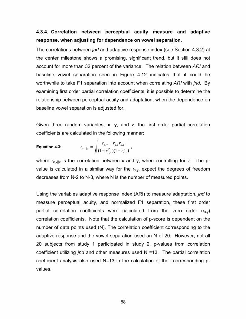
88

4.3.4. Correlation between perceptual acuity measure and adaptive response, when adjusting for dependence on vowel separation.

The correlations between jnd and adaptive response index (see Section 4.3.2) at

the center milestone shows a promising, significant trend, but it still does not

account for more than 32 percent of the variance. The relation between ARI and

baseline vowel separation seen in Figure 4.12 indicates that it could be

worthwhile to take F1 separation into account when correlating ARI with jnd. By

examining first order partial correlation coefficients, it is possible to determine the

relationship between perceptual acuity and adaptation, when the dependence on

baseline vowel separation is adjusted for.

Given three random variables, x, y, and z, the first order partial correlation

coefficients are calculated in the following manner:

Equation 4.3: )1)(1( 2

,2,

,,,||,

zxzy

zxzyyxzyx rr

rrrr

−−

−= ,

where rx,y||z is the correlation between x and y, when controlling for z. The p-

value is calculated in a similar way for the rx,y, expect the degrees of freedom

decreases from N-2 to N-3, where N is the number of measured points.

Using the variables adaptive response index (ARI) to measure adaptation, jnd to

measure perceptual acuity, and normalized F1 separation, these first order

partial correlation coefficients were calculated from the zero order (rx,y)

correlation coefficients. Note that the calculation of p-score is dependent on the

number of data points used (N). The correlation coefficient corresponding to the

adaptive response and the vowel separation used an N of 20. However, not all

20 subjects from study 1 participated in study 2, p-values from correlation

coefficient utilizing jnd and other measures used N =13. The partial correlation

coefficient analysis also used N=13 in the calculation of their corresponding p-

values.

89

Table 4.1 shows the zero order and first order partial correlation coefficients,

utilizing the F1 vowel separation corresponding to the same side as the

perturbation that the subject was exposed to. This table demonstrates that there

is a significant correlation (p < 0.01) between the perceptual jnd of the center milestone and the adaptive response index, when controlling for normalized F1

separation (shown in Table 4.1 at the center set of rows; jnd, ARI || F1 sep.

column). Moreover, this correlation accounts for over 61 percent of the variance

and is negative, indicating that smaller jnd values (i.e. greater perceptual acuity)

are associated with larger adaptation scores. It is also notable that the two other

first order partial correlations are significant, though at a higher significance

threshold (p < 0.05).

The partial correlation coefficients were also calculated for the “same” and

“opposite” milestones, to investigate the possibility that the discrimination index

(i.e. jnd) of these side milestones becomes significantly correlated to adaptation

when F1 separation is controlled for. Table 4.1 shows that this is not the case;

the only significant relation is found between the perception of the the “center”

milestone” and the adaptive response index. (Lack of significant correlation

between non-center milestones and adaptive response was addressed

previously in Section 4.3.2.) zero order rxy first order rxy||z

milestone jnd, ARI F1 sep, ARI jnd, F1 sep jnd, ARI||F1 sep F1 sep, ARI||jnd jnd, F1 sep||ARIr -0.45 0.01 -0.49 0.42 0.22

same r 2 0.21 see below 0.00 0.24 0.18 0.05p-score 0.12 0.97 0.10 0.18 0.50

r -0.57 0.37 0.32 -0.78 0.70 0.69center r 2 0.33 0.13 0.10 0.61 0.50 0.48

p-score 0.04 0.11 0.29 0.00 0.01 0.01

r -0.34 -0.20 -0.29 0.32 -0.09opposite r 2 0.11 see above 0.04 0.08 0.10 0.01

p-score 0.26 0.51 0.36 0.31 0.78 Table 4.1: Partial correlation coefficients, using F1 vowel separation corresponding to the same side of the perturbation. Shown are the correlation coefficients (r) between the parameters indicated in the column headings, square of the correlation coefficient (r2), and the p values for the zero order correlation coefficients (left block) and first order partial correlation coefficients (right block). The top block used the jnd values from the milestone = same condition; the middle used jnd values from the milestone = center condition; and the bottom block used jnd values from the milestone = opposite condition. Significant correlations (p < 0.05) are shown in bold.

90

Table 4.2 is shown below for completeness. It is the same as Table 4.1 but uses

the F1 vowel separation corresponding to the opposite side of the perturbation

that the subject was exposed to. Here, the partial correlation coefficient between

the adaptive response and the jnd at the center milestone, once the F1

separation opposite of the perturbation is controlled for, is the only first order

partial correlation coefficient that is borderline significant (p = 0.05). However,

the p-value for this partial correlation coefficient—p = 0.05—is slightly larger than

the p-value for the correlation coefficient when F1 separation was not controlled

for—p = 0.04—(see Table 4.1); this indicates that jnd and adaptive response

likely do not depend on the F1 separation that is on the opposite side of the

perturbation.

zero order rxy first order rxy||z

milestone jnd, ARI F1 sep, ARI jnd, F1 sep jnd, ARI||F1 sep F1 sep, ARI||jnd jnd, F1 sep||ARIr -0.43 -0.53 -0.32 -0.52

same r 2 see below 0.19 0.28 0.10 0.27p-score 0.14 0.07 0.32 0.09

r -0.06 -0.07 -0.58 -0.12 -0.13center r 2 0.00 0.00 0.33 0.01 0.02

p-score 0.81 0.82 0.05 0.71 0.70

r 0.22 -0.33 0.02 0.21opposite r 2 see above 0.05 0.11 0.00 0.04

p-score 0.48 0.29 0.96 0.51

column repeated in Table 5.1

Table 4.2: Partial correlation coefficients, using F1 vowel separation corresponding to the opposite side of the perturbation. Shown are the correlation coefficients (r), square of the correlation coefficient (r2), and the p-score for the zero order correlation coefficients (left block) and first order partial correlation coefficients (right block). The top block used the jnd values from the milestone = same condition; the middle used jnd values from the milestone = center; and the bottom block used jnd values from the milestone = opposite condition. Redundant information from Table 1 was omitted from this table. No significant correlations (p < 0.05) indicated.

Since Table 4.1 indicates that a significant relation between adaptation and

perceptual acuity exists when the variation due to the produced vowel separation

is factored out, ARI scores were normalized by dividing by F1 vowel separation.

Correlation between this normalized ARI and the perceptual jnd was then

reinvestigated. No significant correlation was found for the “same” (p > 0.4) and

“opposite” (p > 0.3) milestones. However, significant correlation was found

91

between the normalized ARI and the perceptual jnd for the “center” milestone (p

< 0.05), as shown in Figure 4.13.

-0.2 0 0.2 0.4 0.6 0.8 1 1.2 1.4

0.015

0.02

0.025

0.03

0.035

0.04

0.045

milestone = center

ARI/(F1 vowel sep)

jnd

(per

t)

r2 = 0.393, p = 0.021

Figure 4.13: Adaptive response index, normalized by produced vowel separation in F1, is correlated with the jnd score of the center milestone. That is, the 1.0 pert milestone jnd score was used for 0.7 pert (open circles) and 1.3 pert (asterisks) trained subjects. The abscissa is the adaptive response index, divided by the F1 vowel separation, calculated as in Equation 4.3. The ordinate is the jnd (in pert) for the specified milestone, as determined in the “same-different” protocol. Statistics for the regression line are shown in the legend; the p-score reported uses a one-tail test.

4.3.5. Analysis of goodness rating data.

Scores from the goodness rating task (see Section 4.2.5) were analyzed in the

following manner. For each subject, the mean goodness rating value (ranging

from 0 to 7) of the five repetitions for each token was calculated. These values

were then normalized by the subject’s maximum goodness rating value of the

appropriate block: the 0.7 to 1.0 pert block or the 1.0 to 1.3 pert block. A

sigmoid curve was then fit to the data results for each goodness rating block of

each subject; Figure 4.14 shows an example of this analysis for one subject.

92

0.7 0.8 0.9 1

0.1

0.2

0.3

0.4

0.5

0.6

0.7

0.8

0.9

1no

rmal

ized

mea

n go

odne

ss ra

ting

token presented (pert)

AR = 0.18614

1 1.1 1.2 1.3

0.1

0.2

0.3

0.4

0.5

0.6

0.7

0.8

0.9

1

norm

aliz

ed m

ean

good

ness

ratin

g


Figure 4.14: Example of the analysis of the goodness rating task in one subject. Shown is the goodness rating score as a function of the token presented (in pert), for the 0.7-1.0 pert block (left) and the 1.0 to 1.3 pert block (right). The goodness rating scores are the mean value over five repetitions, normalized by the maximum mean value within the block. The error bars are the standard error about the mean. The curve represents the best fit to a sigmoid function. The title over the left block indicates the subject’s adaptive response index score. The ARI is over the left graph, indicating that this subject was run on the 0.7 pert protocol.

Eleven of the thirteen subjects run on the perception protocol had goodness

rating results similar in shape to Figure 4.14. That is, these subjects rated the

tokens near or at 1.0 pert as having the highest goodness rating (normalized

value = 1.0). Two subjects showed goodness rating curves in which the token

rated highest was at the opposite end of the pert continuum as the pert = 1.0

token (see Figure 4.15 and Figure 4.16, left sides). Goodness ratings scores

were subsequently re-measured in both subjects, and they still showed the same

trend (see Figure 4.15 and Figure 4.16, right sides).

93

0.7 0.8 0.9 1

0.1

0.2

0.3

0.4

0.5

0.6

0.7

0.8

0.9

1

1.1

norm

aliz

ed m

ean

good

ness

ratin

g


Outlier1: 1st measure

0.7 0.8 0.9 10.2

0.3

0.4

0.5

0.6

0.7

0.8

0.9

1

1.1

norm

aliz

ed m

ean

good

ness

ratin

g


Outlier1: 2nd measure

Figure 4.15: Analysis of the goodness rating task for outlier subject 1. Refer to Figure 4.14 for axis and legend details.

1 1.1 1.2 1.30.2

0.3

0.4

0.5

0.6

0.7

0.8

0.9

1

norm

aliz

ed m

ean

good

ness

ratin

g


Outlier2: 1st measure

1 1.1 1.2 1.3

0.55

0.6

0.65

0.7

0.75

0.8

0.85

0.9

0.95

1

1.05

norm

aliz

ed m

ean

good

ness

ratin

g


Outlier2: 2nd measure

Figure 4.16: Analysis of the goodness rating task for outlier subject 2. Refer to Figure 4.14 for axis and legend details.

94

Interestingly, outlier subject 2 (Figure 4.16) was also one of the two subjects with

a negative adaptive response (ARI = -0.02). For this subject, the two anomalous

results on the SA and goodness rating tasks may be related. Since this subject

perceives perturbed vowels as “better” vowels, this subject apparently shifted F1

in the same direction as the perturbation. This “positive-feedback loop”

phenomenon is not generally found in other subjects with anomalous results.

That is, the other goodness rating outlier (Figure 4.15) had a positive adaptive

response in the SA protocol; the other subject with a negative adaptive response

had more typical performance on the goodness rating task (with peak rating near

the pert = 1.0 token).

4.3.6. Correlation between goodness rating error and adaptive response.

Measures derived from each subject’s goodness rating curves were calculated to

examine possible cross-subject relations with adaptive response (in a similar

manner to the determination of the relation between jnd and adaptive response in

Sections 4.3.2 to 4.3.4.) One potential property of the goodness rating curve is

category width, defined here as the change in pert corresponding to a criterion

goodness rating score on the best fit goodness rating curve. Defined as such,

category width measures how sharply the category /ε/ is represented on a

goodness rating scale, with smaller category widths corresponding to more

narrow representation of the category. Appendix F shows that, for both

goodness rating blocks (the block on the same side and the block on the

opposite side of the perturbation) at a variety of criterion goodness scores, no

significant correlation was found between category width and adaptive response.

The goodness rating data were also analyzed by examining the amount of

variability within each subject’s goodness rating responses. Specifically, for the

goodness rating block on the same side as the SA perturbation, the standard

error in the subject’s normalized goodness rating score at each pert value was

summed across pert values. The hypothesis here is that subjects with smaller

total error (representing variability in goodness rating) should have greater

95

perceptual acuity, and thus larger adaptive response scores (as discussed in

Section 4.1.1). In the total error goodness rating analysis, the outliers discussed

in Section 4.3.5 were still included (since the direction of their goodness rating

curve does not affect the total variability calculation); however, data from the

subjects with negative adaptive response scores were not used. Figure 4.17

demonstrates that the adaptive response index is significantly correlated with

total goodness rating error (p = 0.05). Moreover, there is a negative relation

between the two, which indicates larger ARI scores are correlated with smaller

values of total error (confirming the perceptual acuity hypothesis).

0.02 0.04 0.06 0.08 0.1 0.12 0.14 0.16 0.18 0.21.1

1.2

1.3

1.4

1.5

1.6

1.7

1.8

1.9

2

2.1


tota

l goo

dnes

s ra

ting

std

erro

r

r2 = 0.360, p = 0.050

Figure 4.17: Adaptive response index is correlated with total goodness rating standard error. The abscissa is the adaptive response index. The ordinate is the sum of the standard error in the rating of each token presented on the goodness rating block. The goodness rating block used is the one corresponding to the same side as the perturbation the subject experienced in the SA protocol. Statistics for the regression line are shown in the legend.

96

4.4. Study 2 summary

The results of study 2 show that perceptual acuity and adaptive response to

perturbations of F1 are significantly related in the manner predicted in Section

4.1.1: subjects with greater perceptual acuity of the acoustic perturbation

demonstrate greater adaptive response. Perceptual acuity of the vowel

perturbation was measured in two ways in study 2: by the index of discrimination

or jnd (refer to Equation 4.1), and by the goodness rating task (refer to Sections

4.3.5 and 4.3.6). The jnd measured at the center milestone was found to be

significantly and negatively correlated with the adaptive response index (Section

4.3.2); this correlation increased once the parameter of baseline vowel

separation was factored out (refer to Section 4.3.4). While the vowel category

width calculated from the goodness rating score was not found to correlate with

adaptation (refer to Appendix E), the total variability in goodness rating scores

was found to be significantly correlated with adaptive response in the negative

direction. Taken together, the results of both perceptual tasks provided evidence

that a subject’s adaptive response increases with greater acuity.

The lack of correlation between vowel category width (as measured with the

goodness rating scores) and adaptive response is not surprising, given the

inherent subjectivity in rating vowels. For example, two subjects who can equally

distinguish the differences vowel acoustics may still rate vowels differently; one

subject may make a conscious decision to ignore these acoustic differences,

while another subject may focus on these differences during the rating process.

In this way, differences in the goodness rating score may not only be due to

differences in perceptual acuity, but also due to a higher-level decision of

whether or not to ignore perceived differences.

The notion of an auditory goal region is important in relating speech perception—

how well one can distinguish differences in the phonemic acoustics—to speech

production. This concept is developed further in the DIVA model simulations

discussed in study 3.

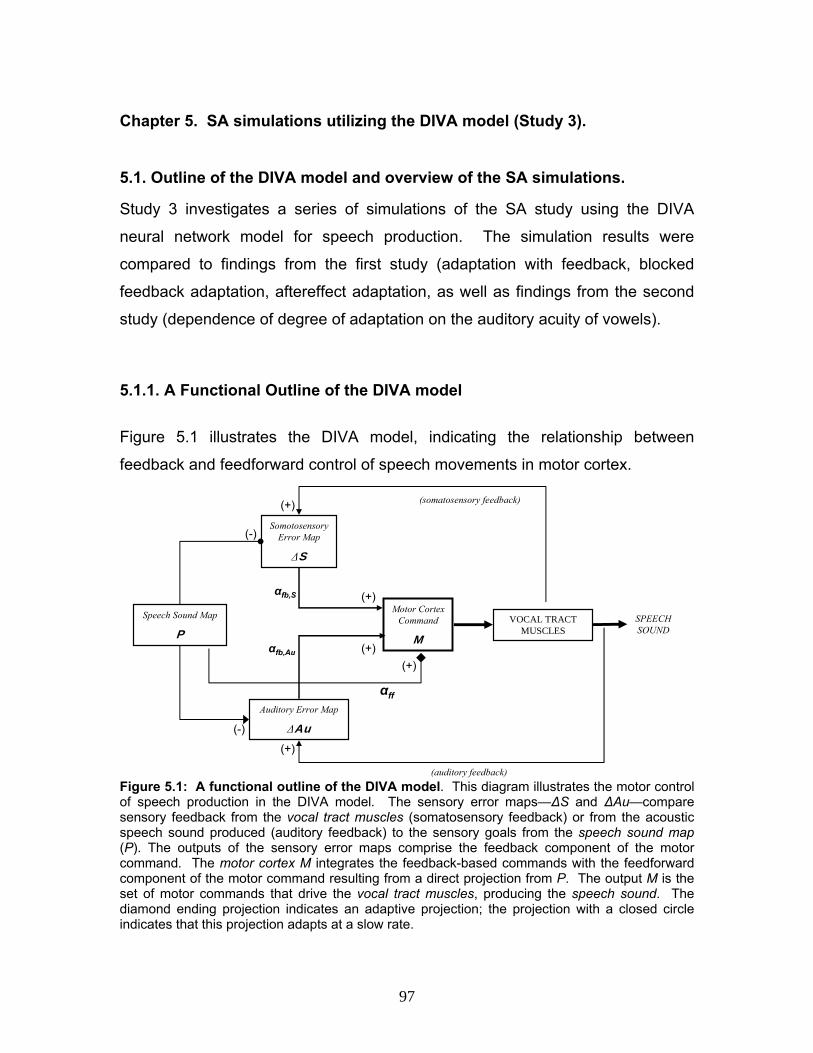
97

Chapter 5. SA simulations utilizing the DIVA model (Study 3).

5.1. Outline of the DIVA model and overview of the SA simulations.

Study 3 investigates a series of simulations of the SA study using the DIVA

neural network model for speech production. The simulation results were

compared to findings from the first study (adaptation with feedback, blocked

feedback adaptation, aftereffect adaptation, as well as findings from the second

study (dependence of degree of adaptation on the auditory acuity of vowels).

5.1.1. A Functional Outline of the DIVA model

Figure 5.1 illustrates the DIVA model, indicating the relationship between

feedback and feedforward control of speech movements in motor cortex.

Speech Sound Map

P

SomotosensoryError Map

ΔS

Auditory Error Map

ΔAu

(-)

(-)

Motor Cortex Command

M

VOCAL TRACT MUSCLES

SPEECH SOUND

(+)

(+)

(auditory feedback)

(somatosensory feedback)

αfb,S

αfb,Au

(+)(+)

αff

(+)

Figure 5.1: A functional outline of the DIVA model. This diagram illustrates the motor control of speech production in the DIVA model. The sensory error maps—ΔS and ΔAu—compare sensory feedback from the vocal tract muscles (somatosensory feedback) or from the acoustic speech sound produced (auditory feedback) to the sensory goals from the speech sound map (P). The outputs of the sensory error maps comprise the feedback component of the motor command. The motor cortex M integrates the feedback-based commands with the feedforward component of the motor command resulting from a direct projection from P. The output M is the set of motor commands that drive the vocal tract muscles, producing the speech sound. The diamond ending projection indicates an adaptive projection; the projection with a closed circle indicates that this projection adapts at a slow rate.

98

The speech sound map (symbolized by P because it is hypothesized to lie in

premotor cortex) projects sensory expectations of the speech feedback

(weighted by zPAu or zPS) to auditory (ΔAu) and somatosensory (ΔS) error cells,

where they are compared to the actual sensory feedback (Au and S in Equation

5.1). Note that the projections of sensory expectations are learned and

continually improve with correct practice (Guenther et al., 2005).

Equation 5.1: )()()()(

)()()()(tztPtAutAu

tztPtStS

PAuPAu

PSPS

δδ−−=Δ

−−=Δ

Here, PSδ and PAuδ represent the transmission delays between the premotor

cortex to somatosensory and auditory cortices, respectively; in the simulations,

these delays are set to 3 msec (Guenther et al., 2005). The weights zPAu encode

the auditory expectations (i.e. the goals), which are hypothesized to be learned

when an infant hears correct productions of speech from other speakers. On the

other hand, the weights zPS encode the somatosensory expectations, and are

presumed to be tuned during correct self-productions. It is important to note that

Equation 5.1 is modified to account for auditory and somatosensory goals that

are not simple point targets, but are goal regions (see Equation 5.7 and Equation

5.8).

The signals resulting from the sensory error cells project to the articulatory

velocity map, resulting in the feedback component of the motor command. These inverse differential kinematics projections are governed by Equation 5.2

(Guenther et al., 2005); here, the gains αfb,Au and αfb,S control how much it

contributes to the overall motor command.

Equation 5.2: )()(

)()(

,,

,,

SMSMSfbSfb

AuMAuMAufbAufb

tSztM

tAuztM

δα

δα

−Δ=Δ

−Δ=Δ

AuMδ and SMδ represent the transmission delays between auditory and

somatosensory cortices and motor cortex, and are again set to 3msec in the

simulations. The weights zAuM and zSM transform the sensory error signals into

corrective motor, and represent pseudoinverse of the Jacobian relating articulator

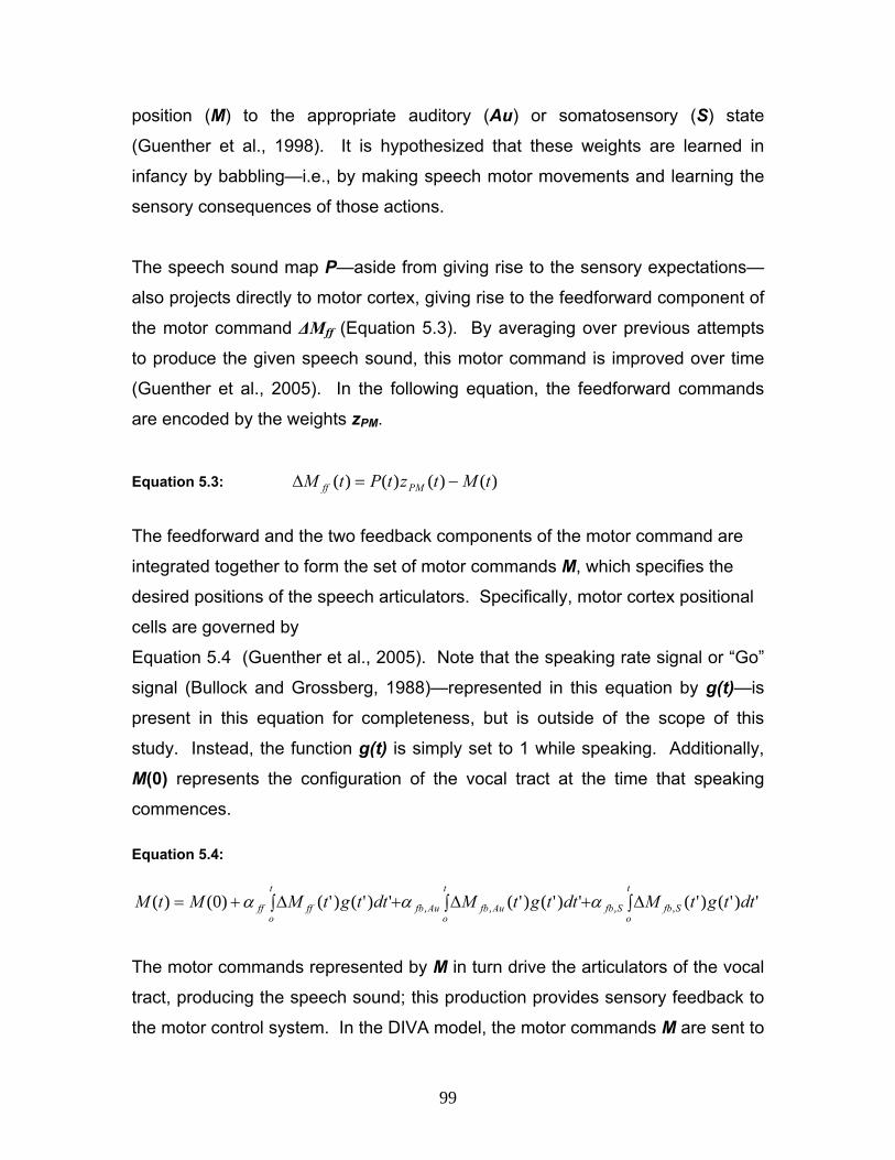
99

position (M) to the appropriate auditory (Au) or somatosensory (S) state

(Guenther et al., 1998). It is hypothesized that these weights are learned in

infancy by babbling—i.e., by making speech motor movements and learning the

sensory consequences of those actions.

The speech sound map P—aside from giving rise to the sensory expectations—

also projects directly to motor cortex, giving rise to the feedforward component of

the motor command ΔMff (Equation 5.3). By averaging over previous attempts

to produce the given speech sound, this motor command is improved over time

(Guenther et al., 2005). In the following equation, the feedforward commands

are encoded by the weights zPM.

Equation 5.3: )()()()( tMtztPtM PMff −=Δ

The feedforward and the two feedback components of the motor command are

integrated together to form the set of motor commands M, which specifies the

desired positions of the speech articulators. Specifically, motor cortex positional

cells are governed by

Equation 5.4 (Guenther et al., 2005). Note that the speaking rate signal or “Go”

signal (Bullock and Grossberg, 1988)—represented in this equation by g(t)—is

present in this equation for completeness, but is outside of the scope of this

study. Instead, the function g(t) is simply set to 1 while speaking. Additionally,

M(0) represents the configuration of the vocal tract at the time that speaking

commences. Equation 5.4:

∫ ∫ ∫ Δ+Δ+Δ+=t

o

t

o

t

oSfbSfbAufbAufbffff dttgtMdttgtMdttgtMMtM ')'()'(')'()'(')'()'()0()( ,,,, ααα

The motor commands represented by M in turn drive the articulators of the vocal

tract, producing the speech sound; this production provides sensory feedback to

the motor control system. In the DIVA model, the motor commands M are sent to

100

an articulatory-based speech synthesizer—the Maeda synthesizer—to produce

speech sounds (Maeda, 1990).

When first learning to speak (corresponding to infant babbling and early word

production), the feedback component of speech control dominates, since the

model has not yet learned feedforward commands for different speech sounds.

With continued speech training, the feedforward projections from the speech

sound map P improve in their ability to predict the correct feedforward

commands. In trained (e.g. adult) speech in normal conditions, feedforward

control dominates the command signal for M cells, since the error signal resulting

from the auditory (ΔAu) and somatosensory (ΔS) error cells is small due to

accurate feedforward commands. In the context of the proposed study,

alterations in auditory feedback cause the feedback control signal (specifically

the auditory component) to increase and significantly influence the overall control

of speech motor cortex. Adaptation occurs in this model as the feedforward

projections remap to account for the acoustic perturbation.

In the current SA protocol, only the auditory component of the sensory feedback

is perturbed; the somatosensory feedback is left unperturbed. Because of

somatosensory feedback, the model predicts that adaptation should not fully

compensate for purely auditory perturbations. That is, modified feedforward

commands will begin to mismatch with previously learned somatosensory goals,

so that the somatosensory error signal counteracts (though not completely) the

effects of the auditory error signal. This prediction is explored further in the

simulations.

5.1.2. Sensory goal regions and auditory acuity in the DIVA model.

One important property of the DIVA model is its reliance on sensory goal regions,

rather than points (Guenther et al., 1998; Guenther, 1995). The notion of

sensory goal regions explains a number of phenomena related to speech

101

production. These properties, which result from auditory goal regions, include

motor equivalent articulatory configurations (Guenther, 1995; Guenther et al.,

1998) and their use in reducing acoustic variability (Guenther et al., 1998;

Guenther et al., 1999a; Nieto-Castanon et al., 2005), as well as anticipatory

coarticulation, carryover coarticulation, and effects related to speaking rate

(Guenther, 1995).

Auditory goal regions also allow the DIVA model to predict the relation (confirmed

by the experimental results in Chapter 4) that subjects with greater acuity—and

thus smaller goal regions—should adapt to a greater extent (see Section 4.1.1).

For computational simplicity, previous versions of the DIVA model used a very

simple notion of the auditory goal regions that were strict “all or nothing” regions.

A more realistic form of the auditory goal regions—one which avoids strict

boundaries—is defined here and used in most of simulation results described in

Section 5.2; simulations results using the “all or nothing” auditory goal regions

are analyzed in Section 5.2.5.

In the new version of auditory goal regions, both the auditory goals G and the

auditory feedback F are modeled as Gaussian distributions (represented by

weights zG and zF, respectively) acting on error cells xi (which are each tuned to

a preferred frequency) as indicated in Equation 5.5.

Equation 5.5: ( )

⎥⎥⎦

⎤

⎢⎢⎣

⎡ −−=

⎥⎥⎦

⎤

⎢⎢⎣

⎡ −−=

2

2

2

2

2exp)(

2)(

exp)(

F

iiF

G

iiG

Fxxz

Gxxz

σ

σ

The auditory acuity of a simulation can be controlled by varying the standard

deviations σG and σF. These values are linearly related to each other, as

specified in Equation 5.6:

Equation 5.6: 1, >∗= σσ σσ kwherek FG

102

The assumption inherent in Equation 5.6—that people with greater discrimination

(smaller σF) will have smaller auditory goals (smaller σG)—is a reasonable one,

given that individuals rely heavily on their perception of the acoustic feedback

when learning their auditory goals. The assumption that σG is greater than σF

effectively encodes the concept that the goals are regions, rather than single

points, in auditory space; that is, more than one value of auditory feedback is

encoded within the goal. Example activation distributions are shown in Figure

5.2.

<G> <F>xi

Figure 5.2: Example of the hypothetical activation distributions, in an auditory dimension. The curves zF (solid) and zG (dashed) represent the activation—as a function of xi (preferred frequency in an auditory dimension)—resulting from the actual feedback and the goal.

Equation 5.7 describes the manner in which the distributions from Equation 5.5

are incorporated in the auditory error calculation. The output activity of a given

cell (term within the numerator summation) consists of the difference between

the activity of the feedback and the goal distributions, with rectification such that

negative values are set to zero; this component makes the output dependent on

the variance of the feedback and goal regions. Such a function could be thought

of as excitatory inputs zF and inhibitory inputs zG acting on a given neuron xi, with

the rectification acting as a threshold value necessary to excite xi. The auditory

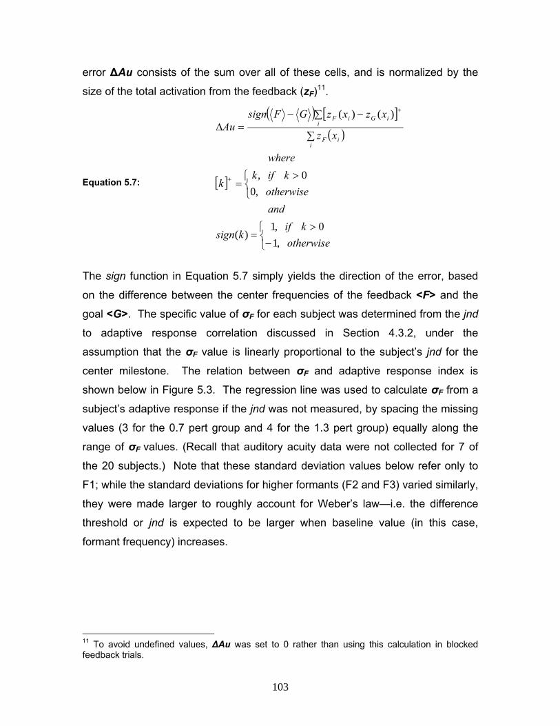
103

error ΔAu consists of the sum over all of these cells, and is normalized by the

size of the total activation from the feedback (zF)11.

Equation 5.7:

( ) [ ]( )

[ ]

⎩⎨⎧−

>=

⎩⎨⎧ >

=

∑

∑ −−=Δ

+

+

otherwisekif

ksign

andotherwise

kifkk

where

xz

xzxzGFsignAu

iiF

iiGiF

,10,1

)(

,00,

)()(

The sign function in Equation 5.7 simply yields the direction of the error, based

on the difference between the center frequencies of the feedback <F> and the

goal <G>. The specific value of σF for each subject was determined from the jnd

to adaptive response correlation discussed in Section 4.3.2, under the

assumption that the σF value is linearly proportional to the subject’s jnd for the

center milestone. The relation between σF and adaptive response index is

shown below in Figure 5.3. The regression line was used to calculate σF from a

subject’s adaptive response if the jnd was not measured, by spacing the missing

values (3 for the 0.7 pert group and 4 for the 1.3 pert group) equally along the

range of σF values. (Recall that auditory acuity data were not collected for 7 of

the 20 subjects.) Note that these standard deviation values below refer only to

F1; while the standard deviations for higher formants (F2 and F3) varied similarly,

they were made larger to roughly account for Weber’s law—i.e. the difference

threshold or jnd is expected to be larger when baseline value (in this case,

formant frequency) increases.

11 To avoid undefined values, ΔAu was set to 0 rather than using this calculation in blocked feedback trials.

104

-0.05 0 0.05 0.1 0.15 0.2 0.255

10

15

20

25

30

35

ARI

σ F for F

1(H

z)0.7 pert1.3 pert

Figure 5.3: Relation between subject adaptive response index (ARI) and model σF value. This plot is similar to Figure 4.8, but the ordinate is rescaled from jnd values on the pert scale to standard deviation values for the auditory activation distributions in Hertz. The cross-labeled values refer to 0.7 pert condition subjects, while the open circles refer to 1.3 pert condition subjects. (Two points, both lying on the regression line, overlapped.) For subjects in which jnd was not measured (gray data points), σF. was distributed evenly along the range of σF. from the regression line.

While the above discussion addresses the calculation of auditory error, the DIVA

model also includes a similar set of calculations for the somatosensory error

cells. However, the focus of the model simulations presented here is to address

adaptation to auditory perturbations, and its relation to auditory acuity.

Additionally, measures were not made regarding subject acuity with regard to

somatosensory dimensions. Thus, somatosensory error is conceptualized here

using a much simpler framework, which has been shown (Guenther et al., 2005)

to replicate human data from experiments utilizing somatosensory perturbations,

such as lip perturbations (Abbs and Gracco, 1984) or jaw perturbations (Kelso et

al., 1984). Specifically, the somatosensory space is composed of dimensions

105

representing proprioceptive information of the current position of the articulators

in antagonistic pairs, as well as dimensions representing palatal and labial tactile

information. The somatosensory error ΔS is simply the difference between the

goal (zPS) and the actual feedback (S); for tactile dimensions, this error is

algorithmically adjusted so that no error results if the actual feedback falls within

a target region (Equation 5.8)12.

Equation 5.8:

⎩⎨⎧ >−−

=Δ

−=Δ

otherwisethresholdzPSSifzPSS

S

zPSSS

tactiletactiletactiletactiletactile

ivepropioceptivepropioceptivepropiocept

,0,

This somatosensory error calculation drives corrective movements which resist

changes in the feedforward command, since such changes will cause

somatosensory error and corresponding corrective movements via the

somatosensory feedback control. Thus the model will not completely

compensate for an auditory perturbation, since the somatosensory feedback will

resist compensatory changes to the feedforward command.

5.1.3. Design of the SA simulations within the DIVA model.

The SA experiment was simulated in the DIVA model as a series of trials under

varying levels of perturbation to the auditory feedback, with one trial in the DIVA

simulation representing one attempt of the DIVA model to produce the given

speech token. To simplify the simulations, the target token the DIVA simulations

produced was solely the phoneme /ε/. Also, the auditory dimensions used in

these simulations were the first three formant frequencies, in units of Hertz13.

Each SA simulation was preceded by a 10 trial speech acquisition period, which

allowed the model to learn the baseline speech target. Following this acquisition

period, the following simulation trials were divided into four phases, similar in

design to the human subject SA experiments: baseline, ramp, full-pert, and post- 12 This threshold represents roughly 2 to 3 percent of the tactile cell’s dynamic range. 13 An alternative representation of the auditory space—using formant ratios—was also considered. However, the use of these auditory dimensions resulted in unintelligible speech productions in pilot studies.

106

pert. Like the human subject experiments, the perturbation used in the full-pert

phase is either 0.7 or 1.3 pert.

After acquisition, auditory feedback was turned on and off to replicate the

+feedback and -feedback SA results. For the vowel /ε/, the human SA

experiment was composed of nine +feedback tokens and three –feedback

tokens. To maintain this ratio, one epoch in the simulation was composed of four

trials: three trials with feedback turned on, followed by one trial with feedback

turned off.

Table 5.1 lists DIVA parameter settings relevant to the SA simulations. While

this table briefly describes these settings, these parameters deserve a little more

discussion.

• αff: This gain controls the contribution of the feedforward command

according to Equation 5.4.

• αfb,Au and αfb,S: These gains control the relative contributions of sensory

error from auditory and somatosensory error cells to the overall feedback

motor command, as according to Equation 5.2. Setting the contribution

from somatosensory error to be smaller than the auditory contribution is

an assumption that should be valid for vowels (e.g. (Guenther et al.,

1998).

• zPAulearning_rate: This learning rate parameters control how fast the

auditory expectations (i.e. goals) change. The learning rate of zPAu is set

to 0, meaning that the auditory goals are invariant once a person has

learned them (presumably early on in life).

• zPSlearning_rate: This learning rate parameters control how fast the

somatosensory goals change. Setting zPSlearning_rate to a small value (e.g.

0.001) indicates that the somatosensory goals are expected to change

very little over the course of a 1.5 hour experiment; the fact that the

somatosensory goals do not change all that much plays an important role

in allowing the SA simulations to recover to baseline in the post-pert

107

phase (see Section 5.2.1). Somatosensory targets are expected to

change slowly over a person’s lifetime to account for developmental

changes in the vocal tract (Callan et al., 2000).

• zPMlearning_rate: This learning rate parameters control how fast the

feedforward commands are updated. Setting zPMlearning_rate to 0.25 (as

opposed to a larger value) allows the feedforward commands to be

learned gradually.

• The inertial dampening terms smooth out sharp movements (which are

likely physiologically unfeasible) by performing the operation in Equation

5.9 at each time step.

Equation 5.9: )(*)1(*)1()( tvalueINERTINERTtvaluetvalue −+−=

αff 1.00 gain for the feedforward command to the overall motor command

αfb,Au 0.95 gain for the auditory component of the feedback command

αfb,S 0.15 gain for the somatosensory component of the feedback command

zPAu learning_rate 0 controls how fast the auditory goals are updated

zPS learning_rate 0.001 controls how fast the somatosensory goals are updated

zPM learning_rate 0.15 controls how fast the feedforward commands are updated

k σ 5.0 linear relation between σG and σ F

FB inert 0.40 inertial dampening of the feedback command

M inert 0.80 inertial dampening of the motor output Table 5.1: Relevant DIVA parameter for the SA simulation. Listed here are the relevant parameters, the values used, and a brief description of the parameter.

Results of the following SA simulations are typically shown as the first formant of

each trial, normalized to the mean of the baseline F1. Some of the following

DIVA model simulations deviated from the standard model parameters outlined

here, as noted in the following text.

108

5.2. DIVA SA simulations results, with comparison to human subject experiments.

5.2.1. DIVA simulations compared with human subject experiments in the +feedback condition.

Results for the DIVA simulations of the SA protocol from +feedback trials are

compared to human subject SA data in Figure 5.4. The simulations were

composed of twenty individual experimental runs, divided into two sets of pert

conditions (either 0.7 or 1.3, just as in the human SA experiments). For a given

set of pert conditions, the only parameter varied was the acuity parameter σF—

using the subjects’ measured or interpolated jnd (see Figure 5.3).

Figure 5.4--shown in normalized first formant values—demonstrates that the SA

simulations account for the human SA data, with F1 changing due to the acoustic

perturbation, then returning to the baseline during the post-pert phase. In this

comparison between SA simulations and human subject experiments, the SA

simulations were able to replicate the full-pert phase of the human subject

results, and in the post-pert phase, the simulations returned by to baseline at a

similar rate to the human subject results. However, at the ramp-phase, the

human SA results seem to show a faster adaptive response than the simulation

results, though this difference is not statistically significant (see below).

Comparing the 0.7 pert group to the 1.3 pert group, it is interesting to note that

there is a slight asymmetry between the two groups, seen in both the simulations

and the human subject results. This is not surprising, given that the inverse of

the perturbation—which represents the maximal response expected—is a larger

change from baseline for the 0.7 pert condition than for the 1.3 pert. To

determine if the simulation results were significantly different than the human

subject results, a pooled, two-tail t-test was performed on an epoch-by-epoch

basis between the two results; significant differences are indicated in Figure 5.4

by the open circles. This figure indicates that the simulations differed

109

significantly from the subject data in only a few baseline epochs. Also, by

comparing the high acuity (solid lines) to the low acuity (dashed lines)

simulations, this figure explicitly demonstrates how acuity and the extent of

adaptation are positively related in the model.

Note that human subjects tended to gradually increase F1 throughout the

baseline (i.e. before the perturbation). The F1 baseline rise is likely a tendency

that research subjects exhibit in the abnormal speaking conditions of the

experimental setup—(c.f. (Jones and Munhall, 2000). Since the model does not

include this tendency, a constant baseline is produced by the model, resulting in

the significant differences between the subjects and the model in the baseline

phase.

10 20 30 40 50 600.85

0.9

0.95

1

1.05

1.1

1.15

1.2

epochs

norm

F1

sig. diff.

Figure 5.4: Normalized F1 during the SA protocol (with feedback), DIVA simulations compared to human subject results. The ordinate corresponds to the adaptive response in the first formant. The abscissa corresponds to the epoch number. The thin lines shown with standard error bars correspond to the human subject SA data (twenty subjects). The lighter shaded region corresponds to the DIVA simulations, and represents the 95% confidence interval about the mean. The vertical dashed lines show the experimental phase transitions, and the horizontal dashed line indicates the baseline. The open circles indicate epochs in which the data and the simulation results are significantly different. The black solid curves correspond to high acuity (i.e. low σF) simulations, while the black dashed curves correspond to low acuity simulations.

110

Simulation and human subject results from the two pert conditions were then

combined by plotting these in adaptive response units, similar to what was done

in study 1 (see Figure 3.10). Shown in Figure 5.5, the simulation results from the

DIVA model compare favorably (as a whole) with human data. Note that only in

one epoch during the ramp phase do the simulation and human data differ

significantly from one another.

10 20 30 40 50 60-0.02

0

0.02

0.04

0.06

0.08

0.1

0.12

0.14

epochs

ARF1

sig. diff.

Figure 5.5: Adaptive response (AR) in F1 during the SA protocol (with feedback), DIVA simulations compared to human subject results. The ordinate corresponds to the adaptive response in the first formant. The abscissa corresponds to the epoch number. The soild lines shown with standard error bars correspond to the human subject SA data (all twenty subjects). The lighter shaded region corresponds to the DIVA SA simulations, and represents the 95% confidence interval about the mean. The vertical dashed lines show the experimental phase transitions, and the horizontal dashed line indicates the baseline. The open circle indicates the only epoch in which the data and the simulation results were significantly different.

5.2.2. DIVA simulations changes with changes in simulation parameters.

The SA simulations shown in Figure 5.5 showed near full recovery to baseline in

the post-pert phase, similar to the human data results. This property depends in

111

part on setting zPSlearning_rate—the learning rate of the expected somatosensory

states—to a small value (0.001). This slow learning rate for zPS allows the

expected somatosensory state of the vowel to remain unchanged throughout the

experiment; when the perturbation is removed in the post-pert phase, the model

thus returns to articulating the vowel as in the baseline phase because it is driven

to minimize both auditory and somatosensory error. To demonstrate the counter-

example, zPSlearning_rate was increased to 0.005 in a set of similar simulations

(Figure 5.6). The increased learning rate in the somatosensory expectations has

the effect of allowing zPS to change more over time as a result of compensation

to the perturbation, rather than act completely resistive. These changes in zPS

prevent F1 from recovering fully (note how ARF1 is elevated above baseline in the

post-pert phase.

10 20 30 40 50 60-0.02

0

0.02

0.04

0.06

0.08

0.1

0.12

0.14

epochs

ARF1

zPSlearn = 0.001

zPSlearn = 0.005

Figure 5.6: Adaptive response (AR) in F1 if the learning rate of the somatosensory goal zPS is increased. This is similar to Figure 5.5, except that adaptive response between simulations with zPSlearning_rate = 0.001 (black) and zPSlearning_rate = 0.005 (gray) are compared. Each curve corresponds to the mean over 20 subjects. Refer to Figure 5.5 for axes details.

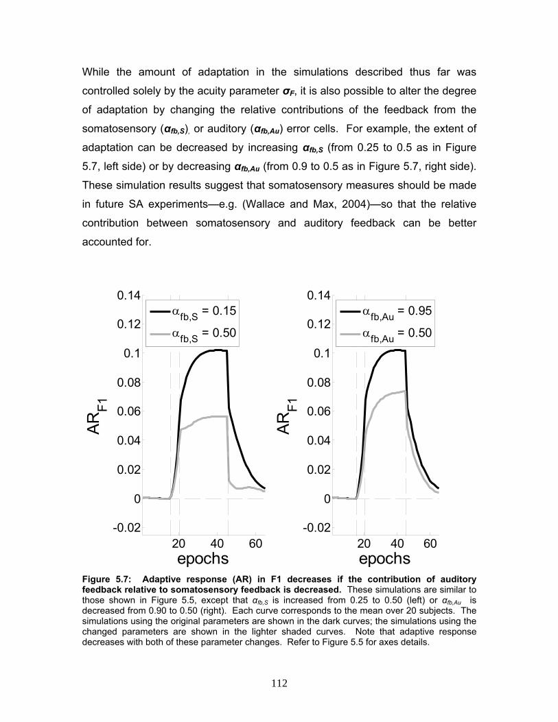
112

While the amount of adaptation in the simulations described thus far was

controlled solely by the acuity parameter σF, it is also possible to alter the degree

of adaptation by changing the relative contributions of the feedback from the

somatosensory (αfb,S), or auditory (αfb,Au) error cells. For example, the extent of

adaptation can be decreased by increasing αfb,S (from 0.25 to 0.5 as in Figure

5.7, left side) or by decreasing αfb,Au (from 0.9 to 0.5 as in Figure 5.7, right side).

These simulation results suggest that somatosensory measures should be made

in future SA experiments—e.g. (Wallace and Max, 2004)—so that the relative

contribution between somatosensory and auditory feedback can be better

accounted for.

20 40 60-0.02

0

0.02

0.04

0.06

0.08

0.1

0.12

0.14

epochs

ARF1

αfb,S = 0.15

αfb,S = 0.50

20 40 60-0.02

0

0.02

0.04

0.06

0.08

0.1

0.12

0.14

epochs

ARF1

αfb,Au = 0.95

αfb,Au = 0.50

Figure 5.7: Adaptive response (AR) in F1 decreases if the contribution of auditory feedback relative to somatosensory feedback is decreased. These simulations are similar to those shown in Figure 5.5, except that αfb,S is increased from 0.25 to 0.50 (left) or αfb,Au is decreased from 0.90 to 0.50 (right). Each curve corresponds to the mean over 20 subjects. The simulations using the original parameters are shown in the dark curves; the simulations using the changed parameters are shown in the lighter shaded curves. Note that adaptive response decreases with both of these parameter changes. Refer to Figure 5.5 for axes details.

113

5.2.3. Changes in the second formant frequency found in the DIVA SA simulations.

To understand how the DIVA simulations model the human changes observed in

the second formant, adaptive response values in F2 for the simulations and

human results are compared in Figure 5.8. The adaptive responses in the

second formant for the DIVA simulations were small, obvious by comparing scale

of Figure 5.8 to that of Figure 5.5, which shows adaptive response in F1.

Moreover, the simulations exhibited changes in F2 that were on the same scale

as seen in the human data. However, the trend of F2 changing in the opposite

direction of F1—observed in the human results (see Section 3.4.2)—was not

observed in these simulations. That is, F2 changed in the positive direction

during the full-pert, which is the same direction as the adaptive response

changes for F1.

10 20 30 40 50 60-0.02

0

0.02

0.04

0.06

0.08

0.1

0.12

0.14

epochs

ARF2

Figure 5.8: Adaptive response in F2 during the SA protocol (with feedback), DIVA simulated subjects compared to human subject results. This is similar to Figure 5.5, but for the second formant adaptive response. The scale of the ordinate is the same as in Figure 5.5.

114

As mentioned earlier, the dimensions for the auditory goals were represented by

formant frequencies, in units of Hertz (see Section 5.1.3). It is possible that

representing the auditory goal regions in an alternative auditory space would

better account for properties related to F2 changes. SA simulations were run

with the auditory spaced represented in Miller formant ratios (Miller, 1989); this

space is define in Equation 3.1. These simulations showed changes in F1 (see

Figure 5.9) that did not follow the human subject results as closely as the

simulations using normal formant auditory dimensions (refer to Figure 5.5).

However, it is interesting to note that F2 for these simulations changes in the

same direction as the human results; that is, in the opposite direction of the F1

changes (see Figure 5.10). Formant ratios have been suggested as a way of

presenting acoustic signals for the same speech sound across speakers; the

present simulation results suggest that a speaker-normalized auditory

representation may explain the F2 results better than the standard formant

representation (Callan et al., 2000).

10 20 30 40 50 600.85

0.9

0.95

1

1.05

1.1

1.15

1.2

1.25

epochs

norm

F1

sig. diff.

Figure 5.9: Normalized F1 in SA results and simulations, from tokens with feedback, using Miller ratio auditory dimensions. This is similar to Figure 5.4, except that the simulations utilized auditory dimensions that were governed by the Miller ratio equations, rather than using formant dimensions in Hertz.

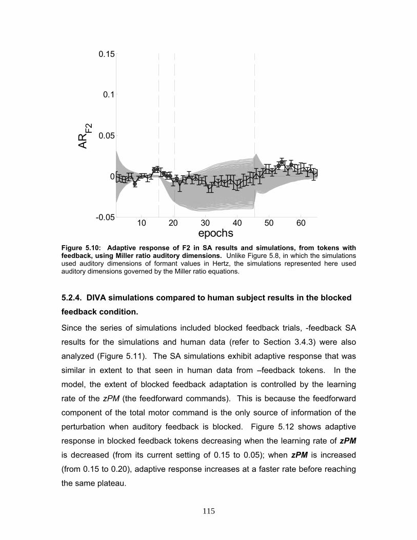
115

10 20 30 40 50 60-0.05

0

0.05

0.1

0.15

epochs

ARF2

Figure 5.10: Adaptive response of F2 in SA results and simulations, from tokens with feedback, using Miller ratio auditory dimensions. Unlike Figure 5.8, in which the simulations used auditory dimensions of formant values in Hertz, the simulations represented here used auditory dimensions governed by the Miller ratio equations.

5.2.4. DIVA simulations compared to human subject results in the blocked feedback condition.

Since the series of simulations included blocked feedback trials, -feedback SA

results for the simulations and human data (refer to Section 3.4.3) were also

analyzed (Figure 5.11). The SA simulations exhibit adaptive response that was

similar in extent to that seen in human data from –feedback tokens. In the

model, the extent of blocked feedback adaptation is controlled by the learning

rate of the zPM (the feedforward commands). This is because the feedforward

component of the total motor command is the only source of information of the

perturbation when auditory feedback is blocked. Figure 5.12 shows adaptive

response in blocked feedback tokens decreasing when the learning rate of zPM is decreased (from its current setting of 0.15 to 0.05); when zPM is increased

(from 0.15 to 0.20), adaptive response increases at a faster rate before reaching

the same plateau.

116

10 20 30 40 50 60-0.05

0

0.05

0.1

0.15

epochs

ARF1

sig. diff.

Figure 5.11: Adaptive response (AR) in F1 for blocked feedback trials, DIVA simulated subjects compared to human subject results. This figure is similar to Figure 5.5, but for blocked feedback trials/tokens (rather than +feedback trials/tokens). The scale of the ordinate is the same as in Figure 5.5.

10 20 30 40 50 600

0.02

0.04

0.06

0.08

0.1

0.12

epochs

ARF1

zPMlearn = 0.05

zPMlearn = 0.15

zPMlearn = 0.20

Figure 5.12: Adaptive response in blocked auditory feedback tokens changes with changes in zPMlearning_rate. Each curve corresponds to the mean over 20 subjects. The thick curve shows the default setting for the learning rate of zPM. Blocked feedback adaptation decreases by decreasing this learning rate (light gray curve), while it increases by increasing this learning rate (dark gray curve).

117

5.2.5. Comparison with a simple conceptualization of the auditory goal regions (the “all or nothing” approach).

Previous versions of the DIVA model implemented a much simpler

conceptualization of auditory goal regions (Guenther, 1995; Guenther et al.,

1998; Guenther et al., 2005), in which no auditory feedback error resulted if the

actual feedback fell within the goal region (i.e. the goal region acted as a “dead

zone” with respect to feedback error). Algorithmically, this concept of the

auditory goal region can be implemented in DIVA as according to the following

equation:

Equation 5.10: ⎪⎩

⎪⎨

⎧<−>−

=Δotherwise

AuUBAuUBAuLBAuLB

Au,0

,,

The action of the auditory error cells in this version of the DIVA model corrects

for sensory errors only up to the boundaries of the goal region, rather than all the

way up to the center of the goal region (as is the case for the Gaussian targets

described in Section 5.1.2) . As shown in Figure 5.13, having the target

boundaries widely separated (dotted line) results in a smaller magnitude auditory

error signal (and thus smaller ΔMfb,Au) when compared to more narrowly

separated boundaries (solid line). In the following simulations, subjects of

varying auditory acuity were simulated by varying the separation of the

boundaries of the auditory goal regions. The half-width of the goal regions used

in these simulations were also based on subject jnd scores, and were 0.8 times

the σG values used in the previous simulations.

118

0Au

| Δ A

u|

Figure 5.13: Dependence of the output of auditory error cells on the size of the auditory goal. Shown here is the auditory feedback error (ΔAu) as a function of the auditory feedback (Au), both in one-dimension. The solid line represents the output of ΔAu from a small goal region, while the dotted line represents the output from a large goal region. For reference, the dashed line represents the output for an auditory point target.

The results of DIVA simulations using these auditory goal regions are shown in

Figure 5.14; note that the remaining model parameters (see Table 5.1) were

unchanged from the DIVA simulations described in Section 5.2.1. In comparing

Figure 5.14 to Figure 5.4 (which used auditory goals regions as described in

Section 5.1.2), the two versions of DIVA simulations show striking similarity.

Indeed, plotted on the shown scale, the only major differences between the two

simulations are that the “all or nothing” goal region simulations appear to have a

wider range of responses (exhibited by the wider confidence interval) for the 1.3

pert simulations, and that one epoch during the full-pert phase of the “all or

nothing” simulations was significantly different from the human subject results.

119

10 20 30 40 50 600.85

0.9

0.95

1

1.05

1.1

1.15

1.2

1.25

epochs

norm

F1

sig. diff.

Figure 5.14: Normalized F1 during the SA protocol (with feedback) using “all or nothing” auditory goal regions. This figure is similar to Figure 5.4, except that the simulations shown here used “all or nothing” auditory goal regions, according to Equation 5.10.

One part of the SA protocol in which there would be a predicted difference

between the two auditory goal conceptualizations is during small perturbations.

Simulations using “all or nothing” auditory goals are expected to show no

adaptive response if the actual feedback falls within the auditory goal; the same

is not expected of simulations using Gaussian auditory goals. The simulations

do in fact demonstrate this behavior, as shown in Figure 5.15; the “all or nothing”

simulations show less change in F1 than the Gaussian auditory goal simulations

at the early epochs of the ramp phase. Indeed, for epochs 16 and 17 in the 1.3

pert simulations, no change in F1 is seen in the simulations on the right,

indicating that the perturbation is not large enough to cause the actual auditory

feedback to fall outside the goal region. Given the large adaptive response seen

in the ramp phase of the human SA data, it is likely that auditory goal regions

120

resemble the Gaussian distributions rather than the simple “all or nothing”

regions in the tendency to start adapting to even very small perturbations.

15 16 17 180.99

0.995

1

1.005

1.01

1.015

1.02

epochs

norm

F1

15 16 17 180.99

0.995

1

1.005

1.01

1.015

1.02

epochs

norm

F1

Figure 5.15: Comparison of normalized F1 during the early part of the ramp-phase between simulations using goal regions that are Gaussian (left) or “all or nothing” (right). The solid lines indicate the mean normalized F1 value for 0.7 pert simulations (upper) and 1.3 pert simulations (lower). The shaded regions indicate +/- one standard error. The vertical dashed line indicates the start of the ramp phase, while the horizontal dashed line indicates the baseline.

5.3. Study 3 Summary.

In the series of simulations presented here, the DIVA model was able to

quantitatively account for a number of characteristics of the human subject SA

studies. The DIVA simulations demonstrated adaptation to acoustic

perturbations (Figure 5.4 & Figure 5.5). This adaptive response was retained

when feedback was turned off in a similar manner to human SA data (Figure

5.11) and demonstrated greater specificity for F1—the formant perturbed in the

SA protocol—than for F2 (Figure 5.8). Individual auditory acuity for vowels is

121

accounted for in DIVA by the auditory goal regions, which are smaller in

individuals with greater acuity.

Differences between the DIVA simulations and human subject data have

suggested possible ways in which DIVA may be modified to better model the

speech production system. For example, the simulation results suggest that the

interaction between somatosensory feedback and auditory feedback will

significantly affect the degree of adaptation (see Figure 5.7). However, the

current DIVA simulations were run using the assumption that the relative weight

of somatosensory and auditory feedback (αfb,S and αfb,Au) are constant from

subject to subject, an assumption that may not necessarily be valid and should

be measured. Additionally, results from the Miller ratio simulations (Figure 5.10)

suggest that changes to the model’s auditory representation to account for

speaker normalization may provide a better explanation for the direction of

change of F2 in response to perturbations in F1.

An additional discrepancy between the simulation results and the human subject

results is during the ramp-phase: human subjects appear to react more quickly

to the perturbation than the simulations do, though this difference did not reach

statistical significance in most epochs. There may be a number of methods to

improve the model’s performance to small perturbations. The manner in which

auditory goal regions are implemented in the model may need to be modified.

For example, the shape of the activation distributions zG and zF could be

changed (they are currently modeled as Gaussian functions) to another function

that may allow greater adaptive response to small perturbations than was seen in

Figure 5.15. Another possibility is that the auditory error calculation occurs as a

two-stage process, rather than the one-stage process described here. Earlier

versions of the DIVA model hypothesized that projections from sensory error

cells to motor cortex had cortico-cortical components (as described in Section

5.1.1), as well as cerebellar ones (Guenther and Ghosh, 2003). A two-stage

feedback control process, with each stage differing in sensitivity to changes in

122

phoneme acoustics, may be able to account for the sensitivity to small acoustic

perturbations demonstrated by subjects participating in study 1. However, it

should be noted that fMRI experiments studying the regions of the brain that are

active during unexpected auditory perturbations (Tourville et al., 2005) did not

find regions of the cerebellum active during perturbations, thus supporting the

hypothesis that sensory error cells utilize only the cortico-cortical pathway.

123

Chapter 6. Overall summary and future directions.

6.1. Overall research summary.

The intent of the research in this thesis was to study the auditory feedback

component of speech motor control with an experimental protocol that caused

subjects to adapt to perturbations in their auditory feedback. Study 1 extensively

investigated the responses of human subjects in a speech sensorimotor

adaptation protocol, addressing issues such as adaptation specificity (changes in

unperturbed auditory dimensions such as F0 or F2); adaptation persistence when

feedback is blocked and when the perturbation is removed; and generalization to

untrained vowels or phonetic context. In study 2, perceptual acuity for some of

the study 1 subjects was measured in two ways: in a discrimination protocol and

in a goodness rating task. Analysis of the acuity measures showed that subjects

with greater acuity for the acoustic perturbation demonstrated greater adaptive

response, and this relation was statistically significant. DIVA model simulations

of the sensorimotor adaptation experiments were able to accurately capture

many aspects of the human subject results (study 3).

The analysis of this thesis research illuminated a number of assumptions that the

DIVA model simulations used to replicate the results of the SA experiment. The

variations of the sensorimotor adaptation experiment proposed here are

designed to better understand the validity of these assumptions, as well as to

allow for further refinement of the DIVA neural network model. Possible ways the

DIVA model may be improved are discussed in the following.

6.2. The role of somatosensory feedback.

In the previous DIVA simulations, the weight of somatosensory feedback control

(αfb,S) relative to auditory feedback control (αfb,Au) was presumed to be the same

across subjects. This is not necessarily a valid assumption; moreover, since

somatosensory feedback can influence the extent of adaptation in DIVA

124

simulations (see Section 5.2.1), it is possible that differences in somatosensory

feedback can account for some of the inter-subject variation seen in adaptation.

One possible way to determine the relative contributions of somatosensory and

auditory sensory information to the overall feedback motor control command is in

an experiment which incorporates conflicting perturbations in both sensory

dimensions. Colleagues have developed a jaw-perturbation apparatus

(henceforth referred to as the “Perturbatron”), which consists of a solenoid-driven

air cylinder that delivers pneumatic pressure to a small balloon placed between

the subjects molars (Tourville et al., 2004). Jaw height can be used to control

first formant frequency: vowels with a high F1 (such as /æ/) are articulated with a

low jaw height while low F1 vowels (such as /I/) are articulated with a high jaw

height. By using the Perturbatron in conjunction with F1 formant shifted acoustic

feedback such that subjects get contradictory somatosensory and auditory

feedback concerning F1, it would be possible to measure the degree to which the

jaw perturbation inhibits adaptation to acoustic perturbations. The extent of this

inhibition can give insight into how auditory feedback and somatosensory

feedback interact in speech motor control. It would also be interesting to study

subject acuity to somatosensory feedback, in a manner analogous to the way

auditory acuity was studied in Study 2. As mentioned in Section 5.1.2,

somatosensory error in the simulations was calculated in a simpler manner than

auditory error because subject somatosensory acuity data did not exist.

6.3. SA experiments using acoustic perturbations of other acoustic cues.

Shifts in vowel F1 (as used in this specific acoustic perturbation algorithm)

correspond to tongue body height movements (Stevens, 1998). Specifically,

shifting F1 about /ε/—a [-high, -low] vowel—altered the sound towards /æ/—a

[-high, +low] vowel—for F1 increases, or altered it to sound like /I/—a [+high,

-low] vowel. A similar SA experiment might be carried out which studies subject

responses to second formant (F2) shifts, with the hypothesis that subjects should

125

demonstrate adaptive responses in F2 in an equivalent manner that was shown

in study 1. However, this experiment lacks the symmetry in phonetic

representation of F2 shifts that exists for shifts in F1 of /ε/. Whereas shifting F2

up for a [+back] vowel can cause it to be perceived as a [-back] vowel, shifting F2

down for the same vowel does not lead to a perception of different vowel

perception (Stevens, 1998). Indeed, the fact that F2 is already low in [+back]

vowels may present a constraint for subjects in their adaptive response. (Note

that a similar problem is posed for F2 shifts in [-back] vowels

Another future SA experiment could use a similar F1 shift, but centering the shift

on the [+back] vowel /o/; /ε/ is a [-back] vowel. Again, the hypothesis is that

subjects should demonstrate adaptation in the same way as shown in study 1.

This SA experiment would require modification to the F1 perturbation algorithm to

improve F1 detection, since [+back] vowels have low F2 values that have the

potential of being falsely detected as F1. Further, this acoustic perturbation

algorithm might also be used to study adaptive responses to third formant (F3)

perturbations in the phoneme /r/—which is acoustically distinctive by a drop in F3

(Boyce and Espy-Wilson, 1997). The approach could also be broadened by

introducing acoustic perturbations of the acoustics of consonants.

Taken together, such SA experiments would test the robustness of the

hypothesis that speech motor planning makes use of sensory goal regions.

6.4. Neuroanatomic loci of sensory error cells.

Aside from functionally describing the speech motor control system, the DIVA

model also predicts the anatomic locations of the neural cells that make up this

system (Guenther et al., 2005; Guenther and Ghosh, 2003). Functional magnetic

resonance imaging (fMRI) techniques have been useful in identifying the areas of

brain (both cortical and cerebellar) active during overt speech production (Hickok

and Poeppel, 2000); such an fMRI study of simple syllable productions has found

126

supporting evidence for a number of the model’s anatomic predictions (Guenther

et al., 2005). Recent research utilizing the aforementioned Perturbatron with

fMRI techniques has been used to determine areas of the brain that may act as

somatosensory error cells (Tourville et al., 2004). The results of this experiment

corroborate the model’s prediction of somatosensory error cells located in the

supramarginal gyrus. Further, recent fMRI work uses an acoustic perturbation

processor comparable to the one used in Study 1 to determine areas of the brain

that may act as auditory error cells during unexpected auditory perturbations

(Tourville et al., 2005). Again, the model’s prediction, this time of auditory error

cells in the posterior superior temporal gyrus were supported. Findings from

other imaging studies support this hypothesis, including the activity of this same

region during both speech perception and production (Buchsbaum et al., 2001).

Functional imaging will continue to be an important tool to testing hypotheses of

the speech production model. For example, a current imaging study is

investigating the activity of the brain during sustained (as opposed to

unexpected) auditory perturbations, and utilizes the same acoustic perturbation

processor. Also, if imaging data could be obtained in conjunction with the

combined articulatory and acoustic perturbation experiment (proposed in Section

6.2), the activation in each sensory error cell region may provide better insight

into the relation between somatosensory and auditory feedback.

6.5. Proposed enhancements to the DIVA model.

Some of the human subject results in study 1 (Chapter 3) were not replicated in

the SA simulations, suggesting ways that the DIVA model can be enhanced or

expanded to account for these results. Additionally, differences between the

simulations and the human subject results (Chapter 5) suggest other ways the

DIVA model may be modified to better model human data.

127

The model currently represents different phonetic strings in distinct sound map

cells (Guenther et al., 2005), implying that adaptation will not carry over to

speech sounds that did not experience perturbation. This is clearly not the case

in human subjects: when trained—via a series of words receiving perturbed

feedback—to adapt the vowel /ε/, this adaptation generalized to untrained words

containing this vowel (Section 3.4.3), as well as to words containing untrained

vowels (Section 3.4.4). One way to resolve this issue is to allow interaction

between the sound map cells of different speech sounds, with the amount of

interaction dependent on the amount of similarity between the two speech

sounds.

The fundamental frequency (F0) contour is not controlled by the model; instead,

F0 is given a steady value of 100 Hz throughout all simulations. In-progress

research with the model is focused on allowing the model to vary F0 as an

auditory dimension. Such modification will allow the model to replicate results

from sensorimotor adaptation experiments involving F0, as well as moving the

model toward accounting for the control of prosodic aspects of speech.

Additionally, the SA simulations utilizing Miller formant-ratio theory (see Sections

3.2.3 and 5.2.3) may be more successful in replicating human results if F0 is

allowed to vary, since one of the Miller ratio dimensions involves F0 (see

Equation 3.1).

In its current form, the model is a deterministic one; that is, having no random

variables, the same simulation run multiple times will result in the same

outcome—produced speech sound—every time. Speech production and

perception are to some extent stochastic processes, evident in variation in F1

produced during the baseline of the SA experiment (see Figure 3.8) and in the

probabilistic nature of subject responses during discrimination tasks (see Figure

4.6). Transforming DIVA into a stochastic model will allow it to better reflect

human speech.

128

Appendix A. Summary of terms used in this thesis.

The following are different manifestations of sensorimotor adaptation, as

measured in this thesis, compared with the equivalent terminology used in the

Houde and Jordan SA experiment (Houde and Jordan, 2002).

Terminology used in thesis

Definition Equivalent term used in Houde and

Jordan (2002) +feedback adaptation Compensatory change to an

acoustic perturbation, as measured in tokens presented with acoustic feedback turned on

Compensation

-feedback adaptation Compensatory change to an acoustic perturbation, as measured in tokens presented with acoustic feedback blocked by noise

Adaptation

Generalized adaptation Compensatory change to an acoustic perturbation found in vowels or other phonetic contexts that were only presented with the acoustic feedback blocked by noise

Generalization

Aftereffect adaptation Compensatory change to an acoustic perturbation that persists after the acoustic perturbation is removed

not measured

Within vowel adaptation Compensatory change measured during the token presentation (used in +feedback tokens) that demonstrates a lag in adaptive response

not measured

129

Appendix B. Use of the LPC coefficients to determine and shift F1.

The result of the autocorrelation LPC routine in the formant shifting algorithm

(see Figure 3.2) is an 8th order polynomial that represents of original speech

segment:

Equation B.1: ∑=

−−=8

1

1)(i

ii zazA

where the relation between A(z) and the original, pre-emphasized14 speech

segment X(z) is defined in the following manner:

Equation B.2: )(

)(zA

GzX =

That is, the LPC analysis method assumes that X(z) can be accurately

represented by a gain factor G and the polynomial A(z), which describes only the

poles of X(z). Thus, the assumption in LPC analysis is that the analyzed speech

segment contains no zeros and can be described by an “all-pole” model (Markel

and Gray, 1976).

Equation B.1 can alternatively be written with the roots of A(z) stated explicitly, as

in the following:

Equation B.3: ∏=

−− −−=4

1

1*1 )1)(1()(i

ii zczczA

Since X(z), and thus A(z) are real, the roots of A(z) described in Equation B.3

occur in complex conjugate pairs (e.g. cI and cI*). Equation B.3 is a much more

useful form of A(z), since the absolute value of the angles of the roots

correspond to the formants of the analyzed speech segment (Markel and Gray,

1976). Specifically, a given formant Fn can be determined from the root cn (or

alternatively its complex conjugate cn*) using the following equation:

14 A pre-emphasis filter is applied to the speech segment to transform the speech excitation function, G(z), to a constant gain, G.

130

Equation B.4: ratesamplingFwherecangleF

F SnS

n == ,)(2π

Since the autocorrelation LPC analysis yields the polynomial form of A(z)

(Equation B.1), the roots must be determined using a root-finding algorithm, such

as the Hessenberg QR method (Press et al., 2002). The first formant

corresponds to the root with the smallest absolute angle (Equation B.4).

Moreover, the shifted F1 formant can be determined by altering the angle of the

F1 complex roots. Since the order of the LPC polynomial used in the formant

shifting algorithm is 8th order, and its roots occur in complex conjugate pairs, the

maximum number of formants resolved in this application is 4.

The synthesis of the perturbed speech can be accomplished by “zeroing” out the

poles of the original speech segment defined by A(z) and introducing the new

poles corresponding to the perturbed speech segment (defined as A’(z)):

Equation B.5: )()(')()( zX

zAzAzY =

Figure B.1 shows a graphical representation of this synthesis, and demonstrates

that the poles of 1/A’(z) and the zeros of A(z) corresponding to the unshifted

formants cancel each other out. Therefore, whereas the LPC analysis yielded an

8th order polynomial, the synthesis can be accomplished with only a second order

filter representing A(z) and A’(z) in Equation B.5. Specifically, consider that the

original F1 can be represented by the following complex conjugate root pair, with

Ө corresponding to F1 as in Equation B.4:

Equation B.6: θθ

θθ

sincossincos

* jrrcjrrc

−=

+=

The root pair corresponding to the shifted formant F1’ can also be represented by

substituting Equation B.6 with c’, c*’ and Ө’. Using this representation of the

complex roots of F1 and F1’, Equation B.5 can be rewritten in the following

manner:

131

Equation B.7:

)('cos21

cos21

)()'1)('1(

)1)(1()(

221

221

1*1

1*1

zXzrzrzrzr

zXzczc

zcczzY

−−

−−

−−

−−

+−+−

=

−−−−

=

θθ

-1 0 1

-1

0

1

imag

inar

y

Real

Figure B.1: Graphic depiction of the roots (polar form) corresponding to the original and perturbed speech segments. Each root is shown in polar form, with the complex conjugate pairs mirrored about the Im=0 axis. The perturbed speech synthesizer removes the original formants by zeroing out its corresponding roots A(z) (“o” in the figure). The shifted formants are introduced as the poles of A'(z) (“+” in the figure). This figure shows that, since only F1 is altered, the poles of 1/ A'(z) cancels the zeros of A(z) for every complex conjugate root pair except those corresponding to F1. The solid line shows the angle of the roots corresponding to the original, unshifted F1; the dashed line shows the angle of the roots corresponding to the shifted F1 (here, shifted up).

The formant shifting algorithm implements the filter described by Equation B.7

using a direct form II transposed structure (Oppenheim and Schafer, 1999). The

time domain difference equation corresponding to Equation B.7 is as follows:

132

Equation B.8: ]2[]1[)'cos2(

]2[]1[)cos2(][][2

2

−+−−

−+−+=

nyrnyrnxrnxrnxny

θ

θ

Typical examples spectral analysis of the unperturbed and perturbed (0.7 pert)

vowel /ε/ are shown for comparison in Figure B.2 and Figure B.3, respectively.

The shift of F1 from 535 Hz to 370 Hz represents a change in F1 of 0.69 pert15,

demonstrating that the perturbation algorithm is effectively shifting F1 as

designed. Additionally, the amplitude of the original F1 peak is reduced in

amplitude by 12.5 dB compared to the new (perturbed) F1 peak (see Figure B.3);

this demonstrates that the formant shifting algorithm can adequately attenuate

the original F1 value.

F1 = 535 F2 = 1512

F3 = 2378

Figure B.2: DFT spectrum within an example /ε/ vowel, unperturbed. This spectrum was taken from within the vowel of a speech token digitized directly and recorded from the microphone (pre-DSP perturbation). This analysis was carried out via Pratt v 4.2.17—a speech analysis software package—using the following parameters: Hanning window shape with length of 32 msec, and 6 dB/octave pre-emphasis. The ordinate is in units of dB; the abscissa is in units of Hz. The first three formants are labeled. 15 Formant values were obtained from LPC analysis of each spectra.

133

F1 = 370

F2 = 1505

F3 = 2367F1old

Figure B.3: DFT spectrum within an example /ε/ vowel, perturbed. This spectrum was taken from within the vowel of a speech token directly digitized and recorded at the output of the DSP board, perturbation level set at 0.7 pert. The first three formants, as well as the location of the unperturbed F1 (F1old), are labeled. Refer to Figure B.2 for axes details.

134

Appendix C. Individual adaptive response during the sensorimotor adaptation protocol.

The following figures demonstrate the performance of each subject (id numbers

1-20) run on the sensorimotor adaptation protocol (study 1). Performance is

measured by calculating Adaptive Response (see Equation 3.5) as a function of

epoch number. Tokens used to calculate AR only include the + feedback tokens.

For convenience, each subject’s ARI value is shown in the corresponding title.

10 20 30 40 50 60

-0.20

0.20.4

subject ID 1, 0.7 pert female, ARI = -0.047

10 20 30 40 50 60

-0.20

0.20.4

subject ID 2, 0.7 pert female, ARI = 0.187

10 20 30 40 50 60

-0.20

0.20.4


Ada

ptiv

e R

espo

nse

(AR

)

10 20 30 40 50 60

-0.20

0.20.4


10 20 30 40 50 60

-0.20

0.20.4


epoch number

Figure C.1: Individual adaptive response as a function of epoch number for 0.7 pert SA protocol, female subjects. The ordinate corresponds to the adaptive response, which is the formant (in Hz) normalized to the mean value of epochs 6-15 within the baseline phase, then transformed to highlight changes about the baseline of 1.0 (see 3.4.1 for details). Each data point is the mean value of the nine +feedback words; the error bars depict the standard error about the mean. The horizontal dashed line shows AR = 0.0. The vertical lines show transitions in phase of the SA protocol.

135

10 20 30 40 50 60

-0.20

0.20.4

subject ID 6, 0.7 pert male, ARI = 0.0891

10 20 30 40 50 60

-0.20

0.20.4


10 20 30 40 50 60

-0.20

0.20.4


Ada

ptiv

e R

espo

nse

(AR

)

10 20 30 40 50 60

-0.20

0.20.4


10 20 30 40 50 60

-0.20

0.20.4


epoch number

Figure C.2: Individual adaptive response as a function of epoch number for 0.7 pert SA protocol, male subjects. Refer to Figure C.1 for axes details.

136

10 20 30 40 50 60-0.2

0

0.2

subject ID 11, 1.3 pert female ARI = 0.0651

10 20 30 40 50 60-0.2

0

0.2


10 20 30 40 50 60-0.2

0

0.2


Ada

ptiv

e R

espo

nse

(AR

)

10 20 30 40 50 60-0.2

0

0.2


10 20 30 40 50 60-0.2

0

0.2


epoch number

Figure C.3: Individual adaptive response as a function of epoch number for 1.3 pert SA protocol, female subjects. Refer to Figure C.1 for axes details.

137

10 20 30 40 50 60-0.2

0

0.2


10 20 30 40 50 60-0.2

0

0.2


10 20 30 40 50 60-0.2

0

0.2

subject ID 18, 1.3 pert male, ARI = -0.0143

Ada

ptiv

e R

espo

nse

(AR

)

10 20 30 40 50 60-0.2

0

0.2


10 20 30 40 50 60-0.2

0

0.2


epoch number

Figure C.4: Individual adaptive response as a function of epoch number for 1.3 pert SA protocol, male subjects. Refer to Figure C.1 for axes details.

* * * * * * * * *

Individual subjects generally showed an increase in AR due to the perturbation,

followed by a gradual decrease after the perturbation was removed. The notable

exceptions to this trend were subjects 1 and 18, both of whom showed negative

adaptation. These figures show that there was still wide variation in the extent of

adaptation in all subjects, as well as in the rate of adaptation (how fast subjects

adapted), and in their rate of recovery (how fast subjects reverted to baseline

after the perturbation was removed).

138

Appendix D. Investigation of the influence of the perturbation algorithm on the second formant.

Results from Section 3.4.2 suggest that, while small, there is a significant change

in the second formant (F2) that is related to changes that the sensorimotor

adaptation protocol causes in the first formant (F1). This Section is included to

investigate the possibility that the F2 changes were a result of the signal

processing from the perturbation algorithm (as opposed to actual changes in F2

produced by the subject). If the perturbation algorithm did introduce changes in

F2, then it could be that the inverse relation between F1 and F2 changes seen

during the SA protocol actually resulted from the feedback signal out of the DSP

board, rather than from constraints related to human speech production or

perception.

Certain tokens from the pre-experiment phase of the SA protocol were run with

the perturbation algorithm set at full-pert value, but with the subjects not wearing

the insert earphones (so that the subjects could not hear the perturbed

feedback). In these tokens, F1 and F2 were extracted from both the input signal

to the DSP board (unshifting in F1) and the output signal from the DSP board

(shifted in F1). Changes in F1 caused by the DSP board (calculated as

F1out/F1in) were tested for statistical significance to changes in F2 (F2out/F2in).

The result of this analysis is that no significant correlation between F1 and F2

changes was seen in tokens resulting from the 1.3 pert shift in F1 (p = 0.18), nor

in tokens from the 0.7 pert shift (p = 0.5624). This is evidence that the significant

relation between F1 and F2 changes seen during the SA experiments resulted

from actual subject production

139

Appendix E. Correlation between adaptive response and jnd obtained from staircase protocol only.

The use of a two-stage protocol for measuring jnd was based on the work of

other researchers (Guenther et al., 1999b; Guenther et al., 2004). However,

running this two-stage protocol is time-consuming; on average, the second stage

of the discrimination task took four to five times longer than the first stage (the

adaptive staircase method). Because of this time cost, this analysis investigates

whether the jnd estimated from the first stage is sufficient to find the significant

relations determined when using the more precise (two-stage protocol) jnd

measure.

As Figure E.1 demonstrates, the correlation between jnd and adaptive response

which was significant using the data shown in Figure 4.8 is not significant when

using the one-stage jnd estimate. Furthermore, Table E.1 shows that the

correlation statistics between jnd and ARI measured at all three milestones

worsens when using the one-stage estimate of jnd. Thus, while time-consuming,

these results indicate that the second stage of the discrimination task is

necessary to measure jnd precisely.

140

0 0.05 0.1 0.15

0.03

0.04

0.05

0.06

0.07

0.08milestone = center


jnd,

sta

ge 1

est

. (pe

rt)r2 = 0.095, p = 0.303

Figure E.1: Adaptive response index is not correlated with the 1-stage estimate of the jnd for the center milestone. This plot is similar to Figure 4.8 (which showed a significant correlation). The difference is that the jnd score used here was estimated from the first stage (the adaptive staircase) of the two stage protocol. The abscissa shows the adaptive response index, discussed above. The ordinate is the 1-stage estimate of the jnd (in pert) for the “center” milestone. The statistics for the regression line are shown in the legend; the p-score reported uses a two-tail t-test.

one-stage protocol two-stage protocolsame r2 0.192 0.189

p-score 0.133 0.136

center r2 0.095 0.312p-score 0.303 0.047

opposite r2 0.084 0.088p-score 0.335 0.322

Table E.1: Statistics of correlation between ARI and jnd, one-stage protocol estimate of jnd compared to two-stage protocol jnd measure. The statistics reported are the r2 (square of the correlation coefficient) and the p-score resulting from a one-tail t-test. The center column reports statistics resulting from the correlation between ARI and the one-stage protocol (adaptive staircase) jnd estimate. The right column reports statistics for correlation between ARI and the two-stage protocol jnd measure.

141

Appendix F. Relation between category width and adaptive response. The goodness rating scores determined from the perceptual acuity protocol (refer

to 4.3.5) are used here to determine a measure of the category width for the

unperturbed tokens. Category width is defined here as:

Equation F.1: ⎩⎨⎧

=−=−

==

=

3.1,17.0,1

_7.0

7.0

pertSAifpertpertSAifpert

widthcategorygoodness

goodness

Here, the criterion goodness rating score for all subjects is set at 0.7, since 0.7 is

the lowest score that is common to all subjects analyzed here. Also, though two

sets of goodness rating scores—corresponding to the 0.7 to 1.0 pert block and to

the 1.0 to 1.3 pert block—were measured, the category width is calculated from

the scores corresponding to the same perturbation direction used in the original

SA protocol. (For example, the goodness rating scores for 0.7 pert SA subjects

are calculated from the 0.7 to 1.0 pert block.)

0.7 0.75 0.8 0.85 0.9 0.95 1

0.1

0.2

0.3

0.4

0.5

0.6

0.7

0.8

0.9

1

norm

aliz

ed m

ean

good

ness

ratin

g


category width

Figure F.1: Example of the calculation of category width from the goodness rating scores. The axes are the same as in Figure 4.14. The horizontal dashed line corresponds to the criterion normalized goodness rating score (here, 0.70). The vertical dashed line represents the pert level that intersects the criterion goodness rating score on the best fit curve. This category width is the difference between the intersecting pert level and 1.0.

142

Once the category width is computed, the cross-correlation between this

perceptual property and adaptive response can be examined. Note that,

because of the way the category width is calculated here, data from the two

outlying subjects mentioned in section 4.3.5 were omitted. (These subjects had

goodness rating curves have that increase in rating for tokens increasingly

distant from the pert = 1.0 token.) Like the index of discrimination (jnd), the

vowel category width is inversely related to perceptual acuity; thus, the vowel

category width and adaptive response should be inversely related according to

the relation between acuity and adaptation proposed in Section 4.1.1. However,

Figure F.2 demonstrates that there is not a significant correlation between the

vowel category width and the adaptive response index.

-0.05 0 0.05 0.1 0.15 0.20.1

0.11

0.12

0.13

0.14

0.15

0.16

0.17

0.18

0.19


cate

gory

wid

th

p = 0.545

Figure F.2: Adaptive Response Index (ARI) is not correlated with the category width as determined from the normalized goodness rating scores. The abscissa is the adaptive response index. The ordinate is the category width determined from the subject’s normalized goodness rating scores, measured on the block corresponding to the perturbation they were exposed to on the SA protocol. Subjects whose goodness rating scores were atypical (N=2) were not included here. The p-score for the regression line are shown in the legend.

143

The correlations between category width and adaptive response were

determined for a range of criterion values, and were expanded to the category

width corresponding to the goodness rating block that was opposite of the

perturbation. Note that the opposite side goodness rating blocks did not contain

goodness rating curves typical of the outliers described in Section 4.3.5; thus all

13 subjects were used in the calculation of rcat. width, ARI. Also note that the

goodness rating curves derived from the opposite side blocks had 0.6 pert (as

compared to 0.7 pert for the same side block) as the lowest criterion goodness

score that was common in all subjects.

The results of these studies are shown in Table F.1; none of the correlation

coefficients in this table are significant (p < 0.05), though the correlation becomes

nearly significant for at a couple criterion values. Moreover, most of the

rcat.width,ARI calculated for the “same side” category widths are positive (left side of

Table F.1), whereas the relation between category width and adaptive response

is hypothesized to be negative.

same side of SA perturbation opposite side of SA perturbation

criterion r cat. width, ARI p-value criterion r cat. width, ARI p-value* * 0.60 -0.23 0.50* * 0.65 -0.22 0.53

0.70 0.20 0.546 0.70 -0.21 0.540.75 0.32 0.331 0.75 -0.20 0.560.80 0.48 0.135 0.80 -0.19 0.570.85 0.59 0.057 0.85 -0.19 0.580.90 0.59 0.054 0.90 -0.18 0.590.95 0.55 0.083 0.95 -0.18 0.60

Table F.1: Correlation coefficients between category width and adaptive response index (ARI) with p-values for a range of criterion values. The criterion value is the goodness rating score on the subject’s goodness rating curve that is used to determine the category width. The left side of the table uses the category width derived from the goodness rating block on the same side as the perturbation the subject heard during the SA experiment; the right side uses the category width derived from the goodness rating block on the opposite side of the SA experiment perturbation. None of the correlation coefficients are significant. Since analysis of the relation between jnd and ARI showed that the strength of

the correlation between these scores increased when F1 separation was

controlled for (Section 4.3.4), the partial correlation between category width and

144

ARI scores was also calculated with F1 separation controlled for. In this

analysis, only the category widths from the “same-side” of the perturbation

goodness rating scores are considered, since the “opposite-side” goodness

rating scores all have large p-values. As shown in Table F.2, controlling for F1

separation does not alter the p-value greatly, and none of the correlations

become significant (p< 0.05) when the partial correlation is calculated.

partial correlation coefficientcriterion p-value,zero order p-value, partial

* ** *

0.70 0.546 0.5610.75 0.331 0.3640.80 0.135 0.1660.85 0.057 0.0670.90 0.054 0.0530.95 0.083 0.082

Table F.2: Comparison between p-values for correlation coefficients between category width and ARI scores, zero-order correlation compared to the partial correlation with F1 separation controlled for. Only the category widths from the goodness rating scores that were on the same side of the perturbation are considered here. The center column contains the same p-values shown in Table F.2; the right column contains the p-value from the partial correlation (with F1 separation controlled for).

145

Bibliography Abbs JH, Gracco VL (1984) Control of complex motor gestures: Orofacial muscle responses to load perturbations of lip during speech. Journal of Neurophysiology 51(4):705-723.

Atkeson CG (1989) Learning Arm Kinematics and Dynamics. Ann Rev Neurosci 12:157-183.

Baum SR, McFarland DH (1997) The Development of Speech Adaptation to an Artificial Palate. Journal of the Acoustical Society of America 102:2353-2359.

Bedford F (1989) Constraints on learning new mappings between perceptual dimensions. Journal of Experimental Psychology: Human Perception and Performance 15:232-248.

Bhushan N, Shadmehr R (1999) Computational nature of human adaptive control during learning of reaching movements in force fields. Biological Cybernetics 81:39-60.

Blakemore SJ, Goodbody SJ, Wolpert DM (1998) Predicting the consequences of our own actions: the role of sensorimotor context estimation. Journal of Neuroscience 18:7511-7518.

Boyce S, Espy-Wilson CY (1997) Coarticulatory Stability in American English /r/. Journal of the Acoustical Society of America 101:3741-3753.

Buchsbaum BR, Hickok G, Humphries C (2001) Role of left posterior superior temporal gyrus in phonological processing for speech perception and production. Cognitive Science 25:663-678.

Bullock D, Grossberg S (1988) Neural dynamics of planned arm movements: emergent invariants and speed-accuracy properties during trajectory formation. Psychological Review 95:49-90.

Burnett TA, Freedland MB, Larson CR, Hain TC (1998) Voice F0 responses to manipulations in pitch feedback. Journal of the Acoustical Society of America 103:3153-3161.

Callan DE, Kent RD, Guenther FH, Vorperian HK (2000) An auditory-feedback-based neural network model of speech production that is robust to developmental changes in the size and shape of the articulatory system. Journal of Speech, Language, and Hearing Research 43:721-736.

Ghahramani Z, Wolpert DM, Jordan MI (1996) Generalization to Local Remappings of the Visuomotor Coordinate Transformation. Journal of Neuroscience 16:7095-7096.

146

Ghosh, S. S. (2004) Understanding cortical and cerebellar contributions to speech production through modeling and functional imaging. Unpublished doctoral thesis, Boston University

Guenther FH (1995) Speech sound acquisition, coarticulation, and rate effects in a neural network model of speech production. Psychological Review 102:594-621.

Guenther FH, Espy-Wilson CY, Boyce SE, Matthies ML, Zandipour M, Perkell JS (1999a) Articulatory tradeoffs reduce acoustic variability during American English /r/ production. Journal of the Acoustical Society of America 105:2854-2865.

Guenther, F. H. and Ghosh, S. S. (2003) A model of cortical and cerebellar function in speech. Paper presented at 15th ICPhS. Barcelona, 629-633.

Guenther FH, Ghosh SS, Tourville JA (2005) Neural Modeling and Imaging of the Cortical Interactions Underlying Syllable Production. Brain and Language in press.

Guenther FH, Hampson M, Johnson D (1998) A theoretical investigation of reference frames for the planning of speech movements. Psychological Review 105:611-633.

Guenther FH, Husain FT, Cohen MA, Shinn-Cunningham BG (1999b) Effects of categorization and discrimination training on auditory perceptual space. Journal of the Acoustical Society of America 106:2900-2912.

Guenther FH, Nieto-Castanon A, Ghosh SS, Tourville JA (2004) Representation of sound categories in auditory cortical maps. Journal of Speech, Language, and Hearing Research 47:46-57.

Hickok G, Poeppel D (2000) Toward a functional neuroanatomy of speech perception. Trends in Cognitive Sciences 4:131-138.

Honda M, Fujino A, Kaburagi T (2002) Compensatory responses of articulators of unexpected perturbations of the palate shape. Journal of Phonetics 30:281-302.

Houde, J. F. (1997) Sensorimotor Adaptation in Speech Production. Unpublished doctoral thesis, Massachusetts Institute of Technology

Houde JF, Jordan MI (2002) Sensorimotor adaptation of speech I: Compensation and adaptation. Journal of Speech, Language, and Hearing Research 45:295-310.

Houde JF, Jordan MI (1998) Sensorimotor Adaptation in Speech Production. Science 279:1213-1216.

147

Ito M (1974) The control of cerebellar motor systems. In: The Neurosciences: Third Study Program. (Schmitt FO, Worden FG, eds), pp 293-303. Cambridge: MIT Press.

Jones JA, Munhall KG (2000) Perceptual calibration of F0 production: Evidence from feedback perturbation. Journal of the Acoustical Society of America 108:1246-1251.

Kawahara H (1993) Transformed auditory feedback: Effects of fundamental frequency perturbation. ATR Human Information Processing Research Laboratories.

Kawato M (1999) Forward models for physiological motor control. Current Opinion in Neurobiology 9:718-727.

Kawato M, Gomi H (1992) The cerebellum and VOR/OKR learning models. Trends in Neurosciences 15:445-453.

Kelso JAS, Tuller B, Vatikiotis-Bateson E, Fowler CA (1984) Functionally specific articulatory cooperation following jaw perturbations during speech: Evidence for coordinative structures. Journal of Experimental Psychology 10(6):812-832.

Lane H, Tranel B (1971) The Lombard sign and the role of hearing in speech. Journal of Speech and Hearing Research 14(4):677-709.

Lindblom BEF, Lubker JF, Gay T (1979) Formant frequencies of some fixed-mandible vowels and a model of speech motor programming by predictive simiulation. Journal of Phonetics 7:147-161.

Macmillan NA, Creelman CD (2005) Detection Theory: A User's Guide. Mahwah: Lawrence Erlbaum Associates, Inc.

Maeda S (1990) Compensatory articulation during speech: evidence from the analysis and synthesis of vocal-tract shapes using an articulatory model. In: Speech Production and Speech Modelling. (Hardcastle WJ, Marchal A, eds), pp 131-149. Netherlands: Kluwer Academic Publishers.

Markel JD, Gray AH (1976) Linear prediction of speech. New York: Springer-Verlag.

Max, L., Wallace, M. E., and Vincent, I. (2003) Sensorimotor adaptation to auditory perturbations during speech: Acoustic and kinematic experiments. Paper presented at 15th ICPhS. Barcelona, 1053-1056.

Menard L, Perrier P, Savariaux C (2004) Exploring production-perception relationships for 4-year-old children: A study of compensation strategies to a lip-tube perturbation. Journal of the Acoustical Society of America 115:2629.

148

Menard L, Schwartz J-L, Boe L-J, Kandel S, Vallee N (2002) Auditory normalization of French vowels synthesized by an articulatory model simulating growth from birth to adulthood. Journal of the Acoustical Society of America 111:1892-1905.

Miall RC, Wolpert DM (1996) Forward models for physiological motor control. Neural Networks 9:1265-1279.

Miller JD (1989) Auditory-perceptual interpretation of the vowel. Journal of the Acoustical Society of America 85:2114-2134.

Newman RS (2003) Using links between speech perception and speech production to evaluate different acoustic metrics: A preliminary report. Journal of the Acoustical Society of America 113:2850-2860.

Nieto-Castanon A, Guenther FH, Perkell J, Curtin HD (2005) A modeling investigation of articulatory variability and acoustic stability during American English /r/ production. Journal of the Acoustical Society of America 117:3196-3212.

Oppenheim AV, Schafer RW (1999) Discrete-Time Signal Processing. Upper Saddle River: Prentice Hall, Inc.

Perkell JS (1997) Articulatory Processes. In: The Handbook of Phonetic Sciences (Hardcastle WJ, Laver J, eds), pp 333-370. Oxford, Eng.: Blackwell.

Perkell JS, Guenther FH, Lane H, Matthies M, Perrier P, Vick J, Wilhelms-Tricarico R, Zandipour M (2000) A theory of speech motor control and supporting data from speakers with normal hearing and with profound hearing loss. Journal of Phonetics 28:233-272.

Perkell JS, Guenther FH, Lane H, Matthies ML, Stockmann ES, Tiede M, Zandipour M (2004a) The distinctness of speakers' productions of vowel contrasts is related to their discrimination of the contrasts. Journal of the Acoustical Society of America 116:2338-2344.

Perkell JS, Matthies ML, Tiede M, Lane H, Zandipour M, Marrone N, Stockmann ES, Guenther FH (2004b) The distinctness of speakers' /s/-/sh/ contrast is related to their auditory discrimination and use of an articulatory saturation effect. Journal of Speech, Language, and Hearing Research 47:1259-1269.

Press WH, Teukolsky SA, Vetterling WT, Flannery BP (2002) Numerical recipes in C. Cambridge: Cambridge University Press.

Savariaux C, Perrier P, Orliaguet JP (1995) Compensation strategies for the perturbation of the rounded vowel [u] using a lip tube: A study of the control space in speech production. Journal of the Acoustical Society of America 98:2428-2842.

149

Savariaux C, Perrier P, Orliaguet J-P, Schwartz J-L (1999) Compensation strategies for the perturbation of French [u] using a lip tube. II. Perceptual analysis. Journal of the Acoustical Society of America 106:381-393.

Sinha NK (1994) Control Systems. New Delhi: Wiley Eastern Limited.

Stevens KN (1998) Acoustic Phonetics. Cambridge: MIT Press.

Tourville JA, Guenther FH, Ghosh SS, Bohland JW (2004) Effects of jaw perturbation on cortical activity during speech production. Journal of the Acoustical Society of America 116:2631.

Tourville, J. A., Guenther, F. H., Ghosh, S. S., Reilly, K. J., Bohland, J. W., and Nieto-Castanon, A. (2005) Effects of acoustic and articulatory perturbation on cortical activity during speech production. Paper presented at 11th Annual Meeting of the Organization for Human Brain Mapping. S49.

Vallabha GK, Tuller B (2002) Systematic errors in the formant analysis of steady-state vowels. Speech Communication 38:141-160.

von Helmholtz H (1962) Helmholtz's treatise on physiological optics. New York: Dover Press.

Wallace, M. E. and Max, L. (2004) Internal models of the vocal tract revealed by articulatory adaptation to formant-shifted auditory feedback. Paper presented at From Sound to Sense: 50 Years of Discovery in Speech Communication.

Welch RB (1978) Perceptual modification: Adapting to altered sensory environments. New York: Academic Press.

Xu Y, Larson CR, Bauer JJ, Hain TC (2004) Compensation for pitch-shifted auditory feedback during the production of Mandarin tone sequences. Journal of the Acoustical Society of America 116:1168-1178.

Yates AJ (1963) Delayed auditory feedback. Psychological Bulletin 60:213-232.

150

Biographical Note Virgilio, son of Eugenio and Dulce Villacorta, was born in Berlin, Germany, and grew up for most of his youth in Anaheim, California. He has two younger sisters, Estella and Eugenie. In 1995, the author received a Bachelors of Science in physics with specialization in biophysics from the University of California, San Diego. In 1999, he received a Masters in Medial Sciences from MCP*Hahnemann University. In 2005, he received a Doctor of Philosophy in Speech and Hearing Bioscience and Technology from the Harvard-MIT Division of Health Science and Technology. While at M.I.T., he enlisted in the United States Army Reserves in 2001, and was later commissioned in 2004. In his free time, the author enjoys running, cycling, baseball, and spending time with Jenny.

sensorimotor adaptation to perturbations of vowel

Documents