sensorless and efficiency optimized …sensorless and efficiency optimized induction machine control...

SENSORLESS AND EFFICIENCY OPTIMIZED INDUCTION MACHINE CONTROL WITH ASSOCIATED CONVERTER PWM MODULATION

SCHEMES

A Dissertation

Presented to

The Faculty of the Graduate School

Tennessee Technological University

By

Gan Dong

In Partial Fulfillment

Of the Requirements for the Degree

DOCTOR OF PHILOSOPHY

Engineering

December 2005

ii

CERTIFICATE OF APPROVAL OF DISSERTATION

SENSORLESS AND EFFICIENCY OPTIMIZED INDUCTION MACHINE CONTROL WITH ASSOCIATED CONVERTER PWM MODULATION

SCHEMES

By

Gan Dong

Graduate Advisory Committee:

Dr. Joseph O. Ojo, Chairperson Date

Dr. Ghadir Radman Date

Dr. Sastry Munukutla Date

Dr. Brian M. O'Connor Date

Dr. Mohamed A. Abdelrahman Date

Approved for the Faculty:

Francis Otuonye

Associate Vice President for

Research and Graduate Studies

Date

iii

ACKNOWLEDGEMENTS

I would like to take this opportunity to express my sincere appreciation to all the

people who were directly or indirectly helpful in making this dissertation a success. First

of all I would like to thank my advisor, Dr. Joseph O. Ojo, who is also the chairperson of

my graduate committee, for his expert guidance and patience during the course of the

research. I would also like to thank the other members of my committee, Dr. Ghadir

Radman, Dr. Sastry Munukutla, Dr. Brian M. O'Connor, Dr. Mohamed A. Abdelrahman,

and Dr. Joe N. Anderson for their effort in reviewing and evaluating my work.

I would also like to thank Zhiqiao Wu, Conard Murray, and L.V. Randolph for their

invaluable help during the course of this project. I would like to express my special

thanks to the US Office of Naval Research (ONR), the Department of Electrical and

Computer Engineering and the Center for Energy Systems Research for the teaching and

research assistantship provided during my graduate study.

I express my gratitude to my parents, my wife Dan, and my daughter Yuzhu for

their moral support and encouragement during the course of my Ph.D. program.

iv

TABLE OF CONTENTS

Page

LIST OF FIGURES ........................................................................................................... ix

LIST OF TABLES......................................................................................................... xxiv

CHAPTER 1 ....................................................................................................................... 1

INTRODUCTION .............................................................................................................. 1

1.1 Introduction.............................................................................................................. 1

1.2 Literature Review..................................................................................................... 5

1.2.1 PWM Schemes in Three-Phase and Multi-Phase Voltage Source Inverters .... 5

1.2.2 Induction Motor Control ................................................................................. 10

1.2.3 Efficiency Optimization.................................................................................. 11

1.2.4 Sensorless Control of Induction Machines ..................................................... 13

1.2.5 Overmodulation Technique for VSI ............................................................... 17

1.3 Research Motivation .............................................................................................. 19

1.4 Scope of Work ....................................................................................................... 22

CHAPTER 2 ..................................................................................................................... 25

PWM SCHEMES IN THREE-PHASE AND MULTI-PHASE VOLTAGE SOURCE

INVERTERS..................................................................................................................... 25

2.1 Introduction............................................................................................................ 25

2.2 Carrier-Based PWM............................................................................................... 26

2.3 Space Vector PWM................................................................................................ 31

2.4 Generalized Discontinuous Modulation Scheme................................................... 40

v

Page

2.5 Modulation Scheme for Multi-Phase Systems....................................................... 47

2.5.1 Generalized Complex-Variable Q-D Reference Frame Transformation ........ 49

2.5.2 Modulation Technique for Multi-Phase Converters ....................................... 52

2.5.3 Modulation for Five-Phase Converters........................................................... 54

2.5.4 Modulation for Six-Phase Converters............................................................. 65

2.5.5 Experimental Results ...................................................................................... 74

2.5.6 Modulation Signals Calculation Using Turn-on Times for the Top Devices . 81

2.6 Conclusion ............................................................................................................. 92

CHAPTER 3 ..................................................................................................................... 93

INDUCTION MACHINE MODEL ................................................................................. 93

3.1 Introduction............................................................................................................ 93

3.2 Operation Principle of a Three-phase Induction Motor......................................... 93

3.3 Three-phase Induction Motor Voltage Equations.................................................. 96

3.4 Reference Frame Transformation ........................................................................ 101

3.5 Three-phase Induction Motor Equivalent Circuit ................................................ 104

3.5.1 Induction Machine Model Using Natural Variables..................................... 109

3.5.2 Induction Machine Model Using Flux Linkages .......................................... 112

3.6 Parameters of Induction Machines....................................................................... 113

3.7 Conclusion ........................................................................................................... 118

CHAPTER 4 ................................................................................................................... 119

VECTOR CONTROL OF INDUCTION MACHINE.................................................... 119

4.1 Introduction.......................................................................................................... 119

vi

Page

4.2 Fundamentals of Vector Control.......................................................................... 120

4.3 Vector Control of Induction Machine.................................................................. 122

4.4 Derivation of Indirect Vector Control of Induction Machine.............................. 126

4.5 Input-output Feedback Linearization................................................................... 128

4.6 Formulation of Indirect Vector Control Scheme of Induction Machine.............. 135

4.7 Control Design for Indirect Vector Control Scheme of Induction Machine ....... 139

4.8 Simulation Results ............................................................................................... 145

4.9 DSP Implementation and Experimental Results.................................................. 150

4.9.1 Calculation of Rotor Flux Linkages.............................................................. 150

4.9.2 Per Unit Model and Base Values .................................................................. 156

4.9.3 Voltage / Current Sensing and Scaling ......................................................... 158

4.9.4 Speed Sensing and Scaling ........................................................................... 160

4.9.5 Slip Estimation.............................................................................................. 161

4.9.6 Program Flowchart........................................................................................ 163

4.10 Experimental Results ......................................................................................... 164

4.11 Conclusion ......................................................................................................... 167

CHAPTER 5 ................................................................................................................... 168

EFFICIENCY OPTIMIZING CONTROL OF INDUCTION MOTOR USING

NATURAL VARIABLES.............................................................................................. 168

5.1 Introduction.......................................................................................................... 168

5.2 Induction Motor Model with Core Loss .............................................................. 169

5.3 Natural Variable Model and Total Loss Minimization........................................ 172

vii

Page

5.4 Formulation of Control Scheme........................................................................... 175

5.5 Speed Estimation ................................................................................................. 178

5.5.1 Using Imaginary Power ................................................................................ 178

5.5.2 Using Rotor Voltage Equations .................................................................... 179

5.5.3 Using Rotor Voltage Equations (modified) .................................................. 183

5.6 Simulation Results ............................................................................................... 185

5.7 Experimental Results ........................................................................................... 189

5.8 Loss Minimization Using a Controller for the Loss Minimization Function ...... 198

5.9 Conclusion ........................................................................................................... 201

CHAPTER 6 ................................................................................................................... 203

SPEED ESTIMATION FOR INDUCTION MOTORS USING FULL-ORDER FLUX

OBSERVERS ................................................................................................................. 203

6.1 Introduction.......................................................................................................... 203

6.2 Induction Machine Model.................................................................................... 205

6.3 Full-order Flux Observer and Speed Estimation ................................................. 207

6.4 Theory of MRAS (Model Reference Adaptive System)...................................... 208

6.5 State Error Analysis and Transfer Function for Speed Estimation...................... 213

6.6 Observer Gain Selection ...................................................................................... 218

6.7 D-decomposition Method .................................................................................... 227

6.8 PI Control Parameters Selection .......................................................................... 230

6.9 Formulation of Control Scheme........................................................................... 241

6.10 Simulation Results ............................................................................................. 244

viii

Page

6.11 Conclusion ......................................................................................................... 253

CHAPTER 7 ................................................................................................................... 254

GENERALIZED OVER-MODULATION METHODOLOGY FOR CURRENT

REGULATED THREE-PHASE VOLTAGE SOURCE CONVERTERS..................... 254

7.1 Introduction.......................................................................................................... 254

7.2 Linear PWM Modulation Schemes...................................................................... 255

7.3 Modulation in the Overmodulation Regions........................................................ 259

7.4 Open-loop Voltage Generation ............................................................................ 263

7.5 Current Regulation............................................................................................... 269

7.6 Experimental Results ........................................................................................... 276

7.7 Conclusion ........................................................................................................... 287

CHAPTER 8 ................................................................................................................... 289

CONCLUSIONS AND FUTURE WORK ..................................................................... 289

8.1 Conclusions.......................................................................................................... 289

8.2 Future Work ......................................................................................................... 291

REFERENCES ............................................................................................................... 293

ix

LIST OF FIGURES

Page

Figure 1.1 Schematic diagram of a voltage source inverter............................................... 3

Figure 2.1 A general three-phase voltage source converter............................................. 26

Figure 2.2 Illustration of carrier-based PWM using sine-triangle comparison method. (a)

Modulation signal and carrier (triangle) signal. (b) the switching signal after the

comparison................................................................................................................ 30

Figure 2.3 Carrier-based PWM generation. Ch2: modulation signal for phase A (0.6/div);

Ch3: phase A voltage Va (50V/div); Ch4: line to line voltage Vab (50V/div). ......... 31

Figure 2.4 Transformation between reference frames. .................................................... 33

Figure 2.5 Voltage space vector diagram for three-leg, three-phase voltage source

converter including zero sequence voltages. ............................................................ 35

Figure 2.6a Existence functions of top devices in sectors I, II, III. ................................. 38

Figure 2.6b Existence functions of top devices in sectors IV, V, VI............................... 39

Figure 2.7 Space vector PWM generation. Ch1: reference voltage for phase A (0.6/div);

Ch2: modulation signal for phase A (0.6/div); Ch3: phase A voltage Va (50V/div);

Ch4: line to line voltage Vab (50V/div)..................................................................... 40

Figure 2.8 Time determination in sector I. ...................................................................... 41

x

Page

Figure 2.9 Generalized discontinuous PWM generation using

[ ] )(3cossgn15.0 δωα ++⋅= t : (a) o0=δ ; (b) o30−=δ ; (c) o60−=δ . Ch1:

reference voltage for phase A (0.6/div); Ch2: modulation signal for phase A

(0.6/div); Ch3: phase A voltage Va (50V/div); Ch4: line to line voltage Vab

(50V/div)................................................................................................................... 46

Figure 2.10 Feasible windings connections for five-phase machines : series connection

of machines. .............................................................................................................. 52

Figure 2.11 Feasible windings connections for six-phase machines : series connection of

machines, six and three-phase machines. ................................................................. 52

Figure 2.12 Schematic diagram of a multi-phase voltage source converter. ................... 53

Figure 2.13a Voltage space vector diagrams of a five-phase PWM inverter. (a) 1qdV ; (b)

2qdV . .......................................................................................................................... 57

Figure 2.13b Voltage space vector diagrams of a five-phase PWM inverter. (a) 3qdV ; (b)

4qdV ; (c) oV . .............................................................................................................. 58

Figure 2.14 Synthesis of the fundamental voltage in sector 1. ........................................ 59

Figure 2.15a The space vector voltages for the six-phase converter. (a) 1qdV ; (b) 2qdV . 67

Figure 2.15b The space vector voltages for the six-phase converter. (a) 4qdV ; (b) 5qdV . 68

Figure 2.15c The space vector voltages for the six-phase converter. (a) 3qdV ; (b) oV .... 69

Figure 2.16 Selection of voltage vectors in sector 1........................................................ 70

xi

Page

Figure 2.17 Experimental result for five-phase system when m1 = 0.8. (a) m3 = 0,

5.0=µ ; (b) m3 = 0.2, Vno = 0; (c) m3 = 0.2, 5.0=µ ; (d) m3 = -0.2, Vno = 0; (e) m3

= -0.2, 5.0=µ . Ch1: reference voltage for phase A (0.6/div), Ch2: modulation

signal for phase A (0.6/div); Ch3: phase A voltage (50V/div); Ch4: line to line

voltage Vab (50V/div)................................................................................................ 77

Figure 2.18a Experimental result for five-phase system when m1 = 1. (a) m3 = 0.2, Vno =

0 ; (b) m3 = 0.2, 5.0=µ ; (c) m3 = -0.2, Vno = 0 ; (d) m3 = -0.2, 5.0=µ . Ch1:

Reference voltage for phase A (1.2/div); Ch2: modulation signal for phase A

(1.2/div); Ch3: phase A voltage (50V/div); Ch4: line to line voltage Vab (50V/div).

................................................................................................................................... 78

Figure 2.18b Experimental result for five-phase system when m1 = 1. (a) m3 = 0.2,

o0=δ ; (b) m3 = 0.2, o36−=δ ; (c) m3 = -0.2, o0=δ ; (d) m3 = -0.2, o36−=δ .

Ch1: reference voltage for phase A (1.2/div); Ch2: modulation signal for phase A

(1.2/div); Ch3: phase A voltage (50V/div); Ch4: line to line voltage Vab (50V/div).

( ( )( )[ ]δωµ ++= t5cossgn15.0 )................................................................................ 79

Figure 2.19 Spectrum analysis of the line to line voltage Vad (normalized with respect to

the highest fundamental voltage) in the linear modulation region. (a) m1 = 0.8, m3 =

-0.2; (b) m1 = 0.8, m3 = 0.2. 1: 0=noV ; 2: 5.0=µ ; 3:

( )( )[ ]δωµ ++= t5cossgn15.0 , o0=δ ; 4: ( )( )[ ]δωµ ++= t5cossgn15.0 , o36−=δ .

................................................................................................................................... 80

xii

Page


the highest fundamental voltage) in the over-modulation region. (a) m1 = 1.5, m3 = -

0.2; (b) m1 = 1.5, m3 = 0.2. 1: 0=noV ; 2: 5.0=µ ; 3: ( )( )[ ]δωµ ++= t5cossgn15.0 ,

o0=δ ; 4: ( )( )[ ]δωµ ++= t5cossgn15.0 , o36−=δ . ............................................... 80

Figure 2.21 Switching signals for the top devices in sector 1. ........................................ 82

Figure 2.22 Synthesis of fundamental and third harmonic voltages in a five-phase

system. (a) Synthesizing reference voltage in sector 1 of 1qdV ; (b) Corresponding

voltage vectors in 3qdV . ............................................................................................. 83

Figure 2.23 Experimental result for five-phase system when m1 = 0.7, m3 = -0.2. (a)

5.0=µ ; (b) o0=δ ; (c) o36−=δ ( ( )( )[ ]δωµ ++= t5cossgn15.0 ). Ch1: Reference

voltage for phase A (1.2/div); Ch2: Modulation signal for phase A (1.2/div); Ch3:

Phase A voltage (50V/div); Ch4: Line to line voltage Vab (50V/div). ..................... 88

Figure 2.24 Experimental result for five-phase system when m1 = 0.7, m3 = 0.2. (a)


voltage for phase A (1.2/div); Ch2: Modulation signal for phase A (1.2/div); Ch3:

Phase A voltage (50V/div); Ch4: Line to line voltage Vab (50V/div). ..................... 89


5.0=µ ; (b) o0=δ ; (c) o36−=δ ( ( )( )[ ]δωµ ++= t5cossgn15.0 ). Ch1: reference

voltage for phase A (1.2/div); Ch2: modulation signal for phase A (1.2/div); Ch3:

phase A voltage (50V/div); Ch4: line to line voltage Vab (50V/div). ....................... 90

xiii

Page



voltage for phase A (1.2/div); Ch2: modulation signal for phase A (1.2/div); Ch3:

phase A voltage (50V/div); Ch4: line to line voltage Vab (50V/div). ....................... 91

Figure 3.1 Two-pole, three-phase, wye-connected symmetrical induction motor. ......... 94

Figure 3.2 The equivalent phase circuit model of the induction machine. ...................... 97

Figure 3.3 Transformation between reference frames. .................................................. 101

Figure 3.4 The qd0 equivalent circuit model of the induction machine in the arbitrary

reference frame. ...................................................................................................... 108

Figure 3.5 The phase model of the induction machine.................................................. 113

Figure 3.6 No-load test: (a) Mutual impedance vs phase voltage, (b) equivalent core loss

resistance vs phase voltage. .................................................................................... 115

Figure 3.7 Blocked rotor test: leakage impedance vs phase voltage. ............................ 117

Figure 3.8 The q-d equivalent circuit model of the induction machine including core loss

resistance................................................................................................................. 117

Figure 4.1 Idealized DC machine circuit diagram. ........................................................ 121

Figure 4.2 Phasor diagram of vector control of the induction machine......................... 123

Figure 4.3 Proposed indirect vector control scheme for the induction motor. .............. 139

Figure 4.4 Linearization diagram for current control. ................................................... 141

Figure 4.5 Poles location for 2nd Butterworth polynomial. .......................................... 143

Figure 4.6 Indirect vector control diagram for induction machines. ............................. 145

xiv

Page

Figure 4.7 Starting transients at no-load. (a) Speed command and actual speed; (b)

electrical torque; (c) phase A voltage; (d) phase A current. ................................... 147

Figure 4.8 Response to the load change at steady state. (a) Speed command and actual

speed; (b) electrical torque; (c) phase A voltage; (d) phase A current. .................. 148

Figure 4.9 Response to the speed change after steady state. (a) Speed command and

actual speed; (b) electrical torque; (c) speed command and actual speed; (d)

electrical torque....................................................................................................... 149

Figure 4.10a Comparison of simulations of integration using a pure integrator and a LPF.

(a) 0 ,0 00 == Aα ; (b) 0 ,2 00 == Aπα . ................................................................ 152

Figure 4.10b Comparison of simulations of integration using a pure integrator and a LPF.

(a) 0 , 00 == Aπα ; (b) 5.0 ,0 00 −== Aα . ............................................................ 153

Figure 4.11 Comparison of experimental results of integration using a pure integrator

and a LPF. (a) Estimation of qSλ from ( )qssqs IrV − , Ch1: ( )qssqs IrV − , Ch2: qsλ ; (b)

estimation of qsλ and dsλ using low pass filters, Ch1: qsλ , Ch2: dsλ .................... 154

Figure 4.12 Voltage sensing and scaling block diagram (Vab). ..................................... 158

Figure 4.13 Current sensing and scaling block diagram (Ia).......................................... 159

Figure 4.14 Speed sensing and scaling block diagram. ................................................. 161

Figure 4.15 Program flowchart. ..................................................................................... 163

Figure 4.16 Experimental results: the reference speed and actual speed when the

reference speed is ramped up from 0 to 900rpm. Ch1: reference speed (545rpm/div);

Ch2: actual speed (545rpm/div).............................................................................. 164

xv

Page

Figure 4.17a Experimental results at steady state. (a) Reference and actual d-axis rotor

flux linkages (0.6Wb/div); (b) reference q-axis stator currents (-1.65V, 3A/div); (c)

reference d-axis stator current (-1.65V, 3A/div)..................................................... 165

Figure 4.17b Experimental results at steady state. (a) Q- and d-axis stator current in

stationary reference frame (6A/div); (b) q- and d-axis stator voltages in stationary

reference frame (50V/div)....................................................................................... 166

Figure 4.18 Experimental results for speed regulation between -300rpm and 300rpm.

Ch1: reference speed (273rpm/div); Ch2: actual speed (273rpm/div).................... 167


resistance. (a) Q-axis; (b) d-axis. ............................................................................ 170

Figure 5.2 Control scheme for induction motor with electrical loss minimization strategy.

................................................................................................................................. 178

Figure 5.3 Simulation of the rotor speed estimation including reactive power. (a)

Reference and actual rotor speeds; (b) Reference and actual rotor speeds; (c)

Developed electric torque. ...................................................................................... 180

Figure 5.4 Simulation of the rotor speed estimation using rotor voltage equations. (a)

Reference and estimated rotor speeds; (b) reference and estimated rotor speeds... 182


Reference and estimated rotor speeds; (b) reference and estimated rotor speeds... 184

Figure 5.6 Speed regulation and loss minimization for motor starting from zero speed to

300 rad/sec. (a) Developed torque; (b) reference and actual rotor speeds; (c) rotor

flux linkage; (d) total electric loss. ......................................................................... 185

xvi

Page

Figure 5.7 Speed regulation and loss minimization for changing load torque. (a)

Developed torque; (b) actual and command rotor speed; (c) square of rotor flux

linkage; (d) total electric loss.................................................................................. 187

Figure 5.8 Speed regulation and loss minimization for changing rotor speed. (a)

Developed torque; (b) actual and command rotor speed; (c) square of rotor flux

linkage; (d) total electric loss.................................................................................. 187

Figure 5.9 Response to the speed change after steady state. (a) Reference speed and

actual speeds; (b) electrical torque.......................................................................... 188

Figure 5.10 Actual / estimated rotor speed corresponding to load change. (a) Reference

and estimated speeds; (b) electric torque. ............................................................... 188

Figure 5.11 Speed regulation from zero to 900 rpm. Ch1: reference rotor speed

(545rpm/div); Ch2: actual rotor speed (545rpm/div); Ch3: square of rotor flux

linkage (0.1Wb2/div); Ch4: phase A current (6A/div)............................................ 189

Figure 5.12 Speed regulation and loss minimization for changing rotor speed from zero

to 900-600 rpm. Ch1: reference rotor speed (545rpm/div); Ch2: actual rotor speed

(545rpm/div); Ch3: square of rotor flux linkage (0.1Wb2/div); Ch4: phase A current

(6A/div)................................................................................................................... 190

Figure 5.13 Actual rotor speed and estimated rotor speed (using actual speed as

feedback). Ch2: actual rotor speed (545rpm/div); Ch3: estimated rotor speed

(545rpm/div). .......................................................................................................... 192

xvii

Page

Figure 5.14 Actual rotor speed, estimated rotor speed and filtered estimated rotor speed (

without calculating the derivatives, using actual speed as feedback). Ch2: actual

rotor speed (545rpm/div); Ch3: estimated rotor speed (545rpm/div); Ch4: filtered

estimated rotor speed (545rpm/div). ....................................................................... 193

Figure 5.15 Actual rotor speed, estimated rotor speed and filtered estimated rotor speed

(calculating the derivatives every 4 sampling period, using actual speed as


(545rpm/div); Ch4: filtered estimated rotor speed (545rpm/div). .......................... 194

Figure 5.16 Reference rotor speed, actual rotor speed and estimated rotor speed


feedback). Ch1: reference speed (545rpm/div); Ch2: measured speed (545rpm/div);

Ch4: estimated speed (545rpm/div). ....................................................................... 195



feedback). Ch1: reference speed (545rpm/div); Ch2: measured speed (545rpm/div);


Figure 5.18 Experimental results for sensorless speed control. (a) 300 - 900rpm; (b) 300

- 600rpm. Ch1: reference speed (545rpm/div); Ch2: measured speed (545rpm/div);



(545rpm/div); Ch2: actual rotor speed (545rpm/div); Ch3: square of rotor flux

linkage (0.1Wb2/div); Ch4: phase A current (6A/div)........................................... 197

xviii

Page

Figure 5.20 Speed regulation ( 300 – 600 rpm) showing rotor flux variation. Ch1:

reference speed (273rpm/div); Ch2: estimated speed (273rpm/div); Ch3: rotor flux

linkage (0.1Wb2/div)............................................................................................... 198

Figure 5.21 The structures of controllers....................................................................... 200

Figure 5.22 Schematic diagram of the control algorithm. ............................................. 201

Figure 6.1 Structure of MRAS for speed estimation. .................................................... 209

Figure 6.2 Poles location for 4th Butterworth polynomial. ........................................... 219

Figure 6.3 22211211 ,,, KKKK with respect to 0ω when mL and rr changes

( rad/s 375 rad/s, 377 == re ωω in motoring mode). (a) 11K ; (b) 12K ; (c) 21K ; (d)

22K . Solid line: =mL *mL , =rr

*rr ; Dotted line: =mL 1.25 *

mL , =rr 1.25 *rr ;

Dashdot line: =mL 1.25 *mL , =rr 0.75 *

rr ; Dashed: =mL 0.75 *mL , =rr 1.25 *

rr ;

Solid line (light): =mL 0.75 *mL , =rr 0.75 *

rr . ....................................................... 222


( rad/s 379 rad/s, 377 == re ωω in generating mode). (a) 11K ; (b) 12K ; (c) 21K ; (d)

22K . Solid line: =mL *mL , =rr


mL , =rr 1.25 *rr ;

Dashdot line: =mL 1.25 *mL , =rr 0.75 *

rr ; Dashed: =mL 0.75 *mL , =rr 1.25 *

rr ;

Solid line (light): =mL 0.75 *mL , =rr 0.75 *

rr . ....................................................... 223

Figure 6.5 22211211 ,,, KKKK with respect to 0ω under different operating conditions

( *mm LL = , *

rr rr = , rad/s 390rad/s 360 rad/s, 377 ≤≤= re ωω ). (a) 11K ; (b) 12K ;

(c) 21K ; (d) 22K ...................................................................................................... 224

xix

Page


( *mm LL = , *

rr rr = , rad/s 195rad/s 180 rad/s, 5.188 ≤≤= re ωω ). (a) 11K ; (b) 12K ;

(c) 21K ; (d) 22K ...................................................................................................... 225

Figure 6.7 23t with respect to 0ω under different operating conditions ( *mm LL = ,

*rr rr = , rad/s 390rad/s 360 rad/s, 377 ≤≤= re ωω ). ........................................... 231

Figure 6.8 Relationship between Kwp and Kwi at different slip frequencies.

( rad/s 17rad/s 13- and rad/s 377 ≤≤= se ωω )........................................................ 233

Figure 6.9 Relationship between Kwp and Kwi at different slip frequency. (a) k = 0.0; (b) k

= 0.2; (c) k = 0.4; (d) k = 0.5; (e) k = 0.8; (f) k = 1.0.


Figure 6.10 Relationship between Kwp and Kwi under parameter changes in motoring

mode (k = 0.5, rad/s 71 and rad/s 377 == se ωω ). 1: ** 5.0 ,5.0 mmrr LLrr == ; 2:

** 5.1 ,5.0 mmrr LLrr == ; 3: ** 5.0 ,5.1 mmrr LLrr == ; 4: ** 5.1 ,5.1 mmrr LLrr == . 236

Figure 6.11 Relationship between Kwp and Kwi under parameter changes in generating

mode (k = 0.5, rad/s -13 and rad/s 377 == se ωω ). 1: ** 5.0 ,5.0 mmrr LLrr == ; 2:


Figure 6.12 Structure of PD controller used for speed regulation. ................................ 237

Figure 6.13 Relationship between Kwrd and Kwrp at different slip frequency. (a) k = 0.0;

(b) k = 0.2; (c) k = 0.4; (d) k = 0.5 (e) k = 0.8; (f) k = 1.0.


xx

Page

Figure 6.14 Relationship between Kwrd and Kwrp under parameter changes in motoring



Figure 6.15 Relationship between Kwrd and Kwrp under parameter changes in generating



Figure 6.16 Rotor flux oriented control including full-order flux observer and adaptive

speed estimation...................................................................................................... 242

Figure 6.17 Starting transients and transients after change in load torque. (a) Reference,

actual, estimated speed; (b) developed torque; (c) slip........................................... 245

Figure 6.18 Starting transients and transients after change in load torque: reference,

actual and estimated speeds (a) during starting; (b) after starting; (c) at the steady

state; (d) zoomed around the reference speed......................................................... 247

Figure 6.19 Starting transients and transients after change in load torque. (a) Difference

between actual and estimated q-axis currents; (b) difference between actual and

estimated d-axis currents......................................................................................... 248

Figure 6.20 Starting transients and transients after change in load torque. (a) Regulation

of drλ ; (b) regulation of qrλ ; (c) regulation of Iqs; (d) regulation of Ids.................. 249

xxi

Page

Figure 6.21 No-load flux linkages at steady state. (a) Actual q- and d-axis rotor flux

linkages; (b) estimated q- and d-axis rotor flux linkages........................................ 250

Figure 6.22 Starting transients and transients after change in load torque. (a) Actual and

estimated qsλ ; (b) actual and estimated dsλ ; (c) actual and estimated qrλ ; (d) actual

and estimated drλ .................................................................................................... 251

Figure 6.23 Response to the change in speed. (a) Reference, actual, estimated speed; (b)

developed torque..................................................................................................... 252

Figure 7.1 (a) Schematic diagram of a voltage source inverter, (b) qdo voltages for the

switching states. ...................................................................................................... 258

Figure 7.2 Voltage trajectories in the inverter. (a) Linear region; (b) over-modulation

region I; (c) over-modulation region II. .................................................................. 261

Figure 7.3 Relationship between crossover angle and modulation index in region I. ... 265

Figure 7.4 Relationship between holding angle and modulation index in region II...... 266

Figure 7.5 Relationship between the crossover / holding angle and modulation

magnitude index...................................................................................................... 267

Figure 7.6 Mapping of the reference and actual modulation magnitude index for

operation in the over-modulation region................................................................. 268

Figure 7.7 Diagram of current regulation in all modulation regions. ............................ 273

Figure 7.8 Simulation of current regulation for q- and d-axis currents. (a) Q-axis

reference current; (b) q-axis actual current; (c) the output from the current controller

for q-axis current; (d) d-axis reference current; (e) d-axis actual current; (f) the

output from the current controller for d-axis current. ............................................. 274

xxii

Page

Figure 7.9 Simulation of current regulation. (a) Phase A fundamental current during the

transient; (b) phase A harmonic current during the transient; (c) phase A

fundamental current at steady state in the overmodulation region; (d) phase A

harmonic current at steady state in the overmodulation region. ............................. 275

Figure 7.10a Trajectory of Vq and Vd and the waveforms for Vq and Vd (0.6/div). (a)

Linear modulation region; (b) overmodulation region I. ........................................ 276

Figure 7.10b Trajectory of Vq and Vd and the waveforms for Vq and Vd (0.6/div). (a)

Overmodulation region II; (b) six step operation. .................................................. 277

Figure 7.11 Current regulation using space vector modulation. (a) Linear – over-

modulation region I; (b) linear–overmodulation region II; (c) overmodulation region

I–II. (1) reference q-axis current (3A/div), (2) measured fundamental q-axis current

(3A/div), (3) reference d-axis current (3A/div), (4) measured fundamental d-axis

current (3A/div), (R1) line-line voltage (200V/div), (R2) phase A measured (raw)

current (6A/div). ..................................................................................................... 280

Figure 7.12a Voltage (Vq –Vd) trajectories using space vector modulation (25V/div). (a)

Linear to over-modulation region I transition; (b) linear to over-modulation region II

transition. ................................................................................................................ 282

Figure 7.12b Current waveforms of phase A. (a) Linear modulation region; (b) over-

modulation region I; (c) over-modulation region II. Ch1: reference current

(1.5A/div), Ch2: measured current (1.5A/div); Ch3: fundamental frequency current

(1.5A/div); Ch4: harmonic current (0.6A/div)........................................................ 283

xxiii

Page

Figure 7.13 Current regulation using discontinuous carrier-based modulation with gain

G. (a) Linear – over-modulation region I; (b) linear–overmodulation region II; (c)

overmodulation region I–II. Ch1: reference q-axis current (3A/div); Ch2: measured

fundamental q-axis current (3A/div); Ch3: reference d-axis current (3A/div); Ch4:

measured fundamental d-axis current (3A/div); ChR1: line-line voltage (200V/div),

ChR2: phase A measured (raw) current (6A/div). .................................................. 284

Figure 7.14 Current waveforms of phase A using discontinuous carrier-based modulation

with gain G. (a) Linear modulation region; (b) over-modulation region II; (c) over-

modulation region II. Ch1: reference current (1.5A/div); Ch2: measured current

(1.5A/div); Ch3: fundamental frequency current (1.5A/div); Ch4: harmonic current

(0.6A/div)................................................................................................................ 285

Figure 7.15 Current regulation using discontinuous carrier-based modulation without

gain G. (a) Linear – over-modulation region I; (b) linear–overmodulation region II;

(c) overmodulation region I–II. Ch1: reference q-axis current (3A/div); Ch2:

measured fundamental q-axis current (3A/div); Ch3: reference d-axis current

(3A/div); Ch4: measured fundamental d-axis current (3A/div); ChR1: line-line

voltage (200V/div); ChR2: phase A measured (raw) current (6A/div). ................. 286

xxiv

LIST OF TABLES

Page

Table 2.1 Switching modes of the three-phase voltage source inverter and corresponding

stationary reference frame qdns voltages.................................................................. 34

Table 2.2 Device Switching times expressed in terms of reference voltages................. 42

Table 2.3 Device Switching times expressed in terms of reference line-line voltages... 43

Table 2.4 Average neutral voltage for all sectors ............................................................ 43

Table 2.5 Normalized times when the three top devices are turned on. .......................... 47

Table 2.6a Analysis on Vo1 for Vqd1 (Vqd2 = 0)............................................................... 61

Table 2.6b Analysis on Vo2 for Vqd1 (Vqd2 = 0)............................................................... 61

Table 2.6c Analysis on Voo for Vqd1 (Vqd2 = 0)............................................................... 62

Table 2.7a Analysis on Vo1 for Vqd1 (Vqd2 = 0)............................................................... 63

Table 2.7b Analysis on Vo2 for Vqd1 (Vqd2 = 0)............................................................... 63

Table 2.7c Analysis on Voo for Vqd1 (Vqd2 = 0)............................................................... 64

Table 2.8a Coefficients for Va1, Vb1, Vc1, Vd1, Ve1, Vf1 ................................................... 71

Table 2.8b Coefficients for Va1, Vb1, Vc1, Vd1, Ve1, Vf1 with coefficient α ..................... 71

Table 2.8c Coefficients for Va2, Vb2, Vc2, Vd2, Ve2, Vf2 ................................................... 72

Table 2.8d Coefficients for Va3, Vb3, Vc3, Vd3, Ve3, Vf3................................................... 72

Table 2.8e Coefficients for Va3, Vb3, Vc3, Vd3, Ve3, Vf3 with coefficient α...................... 73

Table 2.9 Calculation of the modulation signals in terms of turn-on times..................... 84

Table 2.10a Calculation of the modulation signals in terms of line to line voltages....... 85

Table 2.10b Calculation of the modulation signals in terms of line to line voltages....... 85

xxv

Page

Table 2.11 Calculation of the modulation signals am in terms of line to line voltages .. 86

Table 3.1 Parameters of the experimental induction motor........................................... 116

Table 7.1 The turn-on normalized times for three top devices ...................................... 257

Table 7.2 The turn-on normalized times for three top devices in the over-modulation

region ...................................................................................................................... 262

1

CHAPTER 1

INTRODUCTION

1.1 Introduction

Induction machines are widely used in the industry, serving as one of the most

important roles during the energy conversion between electrical power and mechanical

power. Based on the functionality, they are classified into two categories: induction

generators and induction motors. Induction generators consume the mechanical energy

and produce electrical power, which find the applications in the standing-alone electrical

power generations and wind farms. Induction motors produce mechanical power while

consuming the electrical power from the grid, which account for more than one half of

the total electrical power consumed. Especially the induction machines with squirrel cage

rotors are the dominant types due to the simple structures, easy connections, robust to

severe operating conditions, low costs, and maintenance free features. They can be found

in the applications as the important driving sources where a certain motion is required

either linear or rotating ones. They are used to drive fans, pumps, compressors, power

tools, mills, elevators, cranes, electrical vehicles, ships, etc.

The induction machines were initially applied in the cases where the speed was not

required to change frequently since they are difficult to control compared with DC

machines. During the last few decades, the feasible control of induction machines

receives a lot of attentions due to the development of power electronics. The DC

machines were applied for high performance speed and torque control since the air-gap

2

flux and armature current are regulated independently. It means that the torque is

proportional to the armature current once the air-gap flux is fixed, which is very easy to

control. The speed then can be regulated by the control of torque. In the induction

machine, however, the torque is the cross-product of air-gap flux and stator currents, both

of which have two axis components expressed in the q-d plane. All of these four

components will affect the torque production if they are not zero, which is the general

case. Apparently controlling the electric toque is much more complicated in the induction

machines.

With the development of power electronics, the power semiconductor devices are

being extensively used in the power electronic converters, which convert power from one

form to another. The fast-switching devices and the techniques of DSP (Digital Signal

Processor) provide the convenient ways to realize the complex control algorithms such

that the induction machines can be controlled in different ways to satisfy certain

requirements. This is done through controlling the voltages (magnitude, frequency and

angle) applied to the machine through a VSI (Voltage Source Inverter) as shown in

Figure 1.1. The VSI is a certain kind of DC/AC converter, which converts the DC voltage

into AC voltage through PWM (Pulse Width Modulation) technique. The modulation

signals are generated from the control algorithm, which are corresponding to the voltages

with certain magnitude, frequency and angle. These signals are then compared with a

high frequency carrier signal to generate the pulses, which are generally positive when

the modulation signals are greater than the carrier signal and negative when the

modulation signals are smaller than the carrier signal. When these pulses are applied to

3

Load

nob

a

c

2Vd

2Vd

apT bpT cpT

cnTbnTanT

Figure 1.1 Schematic diagram of a voltage source inverter.

switch on and off the switching devices, the fundamental voltage that is embedded in the

output voltage pulses will be the same as the desired voltages.

With the help of the control algorithm and voltage source inverter, a torque

expression similar to that of DC machines can be achieved for the induction machine,

which finds a lot of high performance applications. The toque equation can be simplified

if the angle between the stator current and rotor flux linkage vectors is controlled

although the torque is originally the cross-product of these two vectors. For example, if

one of the rotor flux linkage components is regulated to be zero, the torque equation will

change to the product of two components only, one component comes from the rotor flux

linkage and the other one comes from the stator current. The desired torque can be

produced when these two components are regulated separately.

From the application point of view, the vectors in q-d plane are not visible and the

magnitudes of some quantities are of more importance including the flux, current, electric

torque etc. These quantities are all scalars that are independent of any reference frame.

The reference frame is usually selected as the synchronous one, in which all the time

changing quantities in the stationary reference frame become DC quantities

4

corresponding to a particular steady-state operating condition to facilitate the control. The

transformation is then necessary between the stationary reference frame and synchronous

reference frame since the measured quantities and the modulation signals are in the

stationary reference frame. However, these transformations can be saved if it is possible

to use these scalars in the control and everything can be done in the stationary reference

frame.

One of the most popular control objectives is to control the speed of the induction

machine to the reference speed. The speed is generally measured using speed sensors or

calculated from the absolute position sensors. These speed or position sensors are

expensive and thus increase the total cost of the whole drive system. At the same time,

the installation of the speed or position sensors requires more space and increases the

chances of fault and also the complexity of the system. Thus the research on the speed

control of induction machines has moved to the sensorless speed control, which

eliminates the need of installing speed sensor in order to reduce the cost, or for operation

in special conditions. Speed sensorless control is basically the algorithm of speed

estimation that can infer the required measurement from other more easily available

measurements like voltages and currents.

In the normal operation, the induction machines are operated under the rated

condition. However, in the case of emergency or abnormal situations, the induction

machines are required to generate the output that is more than rated. Thus the voltage

source inverter will have to operate into the overmodulation region to get more voltage

output although the output voltages are not pure sinusoidal any more. The extreme case is

that the phase voltages are square waves, in which the fundamental voltages reach the

5

maximum value. Special manners have to be adopted in order to reduce the torque

oscillations due to the introduction of harmonic components in the voltages and currents.

It is expected that the induction machine can still go back to the normal operating

condition once the problem resulting from abnormal operation is fixed. This capability of

operating in the overmodulation region could increase the stability of the whole drive

system and gives more output torque.

1.2 Literature Review

The review on the various works previously done related to the induction machine

control is necessary in the sense of defining the research scope. It is also helpful to find

the appropriate way of conducting current research under the present conditions by

examining different methods since different methods have their own advantages and

disadvantages. The PWM modulation technique is the first that needs to be studied

because it is the basis of implementing the induction machine control. Then different

methods of the induction machine control are discussed. The approaches of loss

minimization and the speed estimation techniques are highlighted. At last the methods

mentioned in the literatures regarding the overmodulation technique are reviewed.

1.2.1 PWM Schemes in Three-Phase and Multi-Phase Voltage Source Inverters

The general three-phase voltage source inverter feeding a three-phase load is shown

in Figure 1.1. The main purpose of this topology is to generate a three-phase voltage

6

source with controllable amplitude, phase angle and frequency. Pulse width modulation

(PWM) techniques used in three phase voltage source converters can be classified into

two categories : carrier-based PWM and space vector PWM. The PWM technique using

sine triangle intersection was first proposed by Schönung and Stemmler in 1964 [2.1].

Due to the ease of implementation, the sinusoidal PWM has been found in a wide range

of applications. However the output range of its linear operation is limited to 78.5 percent

of the maximum fundamental voltage generated by the six-step operation. Thus the usage

of the DC bus voltage is not efficient. Then the direct digital technique or the space

vector modulation technique was proposed by Pfaff, Weschta and Wick in 1982 [2.2].

And the development of micro-controllers made the implementation of direct digital

technique possible at the same time. This scheme became more and more popular due to

its efficient utilization of the DC link voltage, possible optimization of the output

distortion and switching losses, and compatibility with the digital controller. It has been

widely used for high performance three-phase drive systems and it showed that the

absence of neutral current path in star-connected three-phase systems provides the degree

of freedom in determining the duty cycles of the switching devices. This degree of

freedom is achieved by partitioning the two null states. The equivalent degree of freedom

in sine-triangle comparison method is also observed by injection of appropriate zero

sequence signal. Since the voltage between the load neutral and the reference of the DC

source can take any value, this zero sequence signal is used to alter the duty cycle of the

switching devices and alternatively the modulation signals. Appropriate zero sequence

signal injection could increase the linear range of the voltage generation, improve the

waveform quality and reduce switching losses without affecting the effective output. It

7

has been shown that the linear range of the output voltage was increased to 90.7 percent

of the maximum fundamental voltage generated from the six-step operation. Some other

techniques were developed for harmonic elimination in order to suppress the lower

ordered harmonics. The third harmonic injection (THIPWM) techniques explain that by

adding the third harmonic component to the fundamental voltages for a three-phase

inverter [2.3], it is possible to obtain a line-to-line output voltage that is 15 percent

greater than that obtained when pure sinusoidal modulation is employed and the line-to-

line voltage is undistorted.

The discontinuous modulation technique was developed first and illustrated that the

scheme resulted in high voltage linearity range, reduced switching losses, and superior

current waveform. The scheme had a poor performance in the lower modulation region

and it is desirable to operate when the modulation index is relatively high. It is found that

the harmonic loss in the higher modulation region can be greatly reduced by using an

optimal modulation for minimum switching loss. The correlation between the carrier-

based PWM and space vector PWM was established by changing the duty cycle weights

of the zero states. It was proved that the modified space vector PWM could be

implemented as triangle comparison method by adding the zero sequence voltage to the

fundamental voltages. Hava developed a high performance generalized discontinuous

PWM algorithm [2.4], which employed conventional space-vector PWM in the low

modulation region and generalized discontinuous PWM algorithms in higher modulation

region.

Multi-phase electric machines powered with multi-phase converters are being

seriously considered for several high power applications in order to achieve higher torque

8

per ampere and improve system reliability in applications such as aerospace, electric ship

propulsion, electric locomotive, and hybrid electric vehicles. When a converter leg is lost,

multi-phase machines are able to produce a higher fraction of their rated torques with

little pulsations when compared to the three-phase machines. Five and six phase

machines have improved torque capabilities when the stator windings are injected with

phase currents comprising of the fundamental and third harmonic components, which

individually interact with the fundamental and third harmonic airgap flux densities, each

of them produces an average, non-pulsating electromagnetic torque [2.5, 2.11-2.13]. The

third harmonic air-gap flux density is enhanced with the use of concentrated stator

windings in induction machines, the generation of quasi-rectangular back EMF

waveforms in permanent magnet machines or rotor structure configuration in

synchronous reluctance machines [2.6, 2.14-2.15]. Recently, it has been shown that when

inverter fed multi-phase electric machines with either odd or even phase numbers are

connected in series with other machines with same or lower phase numbers, they can be

independently speed controlled using conventional vector control methodology [2.7-2.9].

Applying what is referred to as space vector decomposition technique to the 64

switching states of the six-phase converter, the output voltages are decomposed into three

voltage sets (d-q), (x-y), and (o1-o2) which are used to synthesize three set of balanced

voltages. The time required to turn on selected switching states in each of the converter

sectors to synthesize desired phase voltages for the dual winding three-phase induction

machines are calculated by solving a set of linear voltage averaging equations. For dual

winding machines of [2.17, 2.18], the synthesis of the fundamental phase voltages

corresponding to the (d-q) set and suppressing (setting to zero) the (x-y), and (o1-o2) were

9

considered. Further sequencing of the selected switching states are required in order to

minimize switching losses and improve waveforms in the implementation of the

continuous and discontinuous space vector PWM (SVPWM) [2.18]. Modulation

strategies for a six-phase converter driving various stator winding connections of a three-

phase dual winding induction machine to synthesize fundamental voltages have been

reported [2.19]. In [2.20], the three-phase unified PWM method for three-phase

converters was extended to n-phase inverters to synthesize sinusoidal phase voltages

which were achieved by applying times of available switching states to approximate the

desired phase voltages. Offset voltages comprising of the instantaneous maximum and

minimum values of the phase voltages are added to the modulation signals to improve the

voltage utilization of the dc bus. SVPWM method for five phase machines based on

multiple d-q space concepts was presented to synthesize both balanced five phase

fundamental and third harmonic voltages required to improve torque capability [2.21].

Resolving the 32 states into two d-q different space vectors for the fundamental and third

harmonic voltages, the switching time required for turning on the selected voltage vectors

are calculated for each sector. Furthermore, it is shown that by adding appropriate offset

voltages to the modulation signals corresponding to the fundamental and third harmonic

voltages to produce flat-top modulation waveforms, the converter voltage gain of the

five-phase converter is improved.

10

1.2.2 Induction Motor Control

There are a lot of control schemes applied for the induction motor drives including

the scalar control, direct torque control, adaptive control, and vector / field oriented

control. The vector control of induction machines emerges with the development of

modern power electronics and is very popular since it can be used to get similar

performance as the DC machine. The basic idea of vector control is that the similar

torque expression compared with DC machines can be derived once the air-gap flux is

aligned on one of the two axes in q-d plane, which means one of the two axis flux is zero

(i.e. 0=qλ ). This method can be applied in different reference frames resulting the

stator, air-gap and rotor flux oriented vector control schemes [4.2-4.3].

In the case of induction machines, the rotor flux oriented control is usually

employed although it is possible to implement stator flux oriented and also magnetizing

flux oriented control. The stator / rotor flux linkages of the induction machines are

necessary for the vector control. In terms of the methods of obtaining the flux linkages,

the field oriented induction machine drive systems are classified into two categories : the

direct field oriented system and the indirect field oriented system. In the former case, the

flux quantities (magnitude and angle) are directly measured by using Hall-effect sensors,

search coils, tapped stator windings of the machine or calculated from the so-called flux

model. For the indirect field oriented control system, the magnitude and space angle of

the flux linkages are obtained by utilizing the monitored stator currents and the rotor

speed. The space angle of the flux linkage is then obtained as the sum of the monitored

rotor angle (corresponding to the rotor speed) and the computed reference value of the

11

slip angle (corresponding to the slip frequency). The indirect field oriented control is still

receiving wide attention although some sensorless control strategies have been proposed

in the last few years [4.1-4.4]. The exact estimation of rotor position is one of the key

issues in the vector control system.

The scalar control is receiving some attentions since they can be used for the

efficiency optimization [4.5-4.6]. From the application point of view, only the

magnitudes of some quantities are important including the flux, current, electric torque

etc. These quantities are all scalars that are constants in any reference frame. Using these

quantities as the control variables leads to the scalar control, which can be used for the

loss minimization since the real power and losses are also scalars. One of the advantage

of using the scalars as the state variables is that no reference frame transformation is

required. It is known that the transformation and reverse transformation between the

stationary and synchronous reference frames are necessary since the control is preferred

to be done in the synchronous reference frame while the measured quantities and the

modulation signals are in the stationary reference frame. If all of the state variables are

scalars, it means that these variables can be calculated in the stationary reference frame.

However, there are some disadvantages of the calculations using the AC signals, which

are not desirable since the calculations using AC signals could result into some error.

1.2.3 Efficiency Optimization

Efficiency improvement of motor drives has been an area of active research within

the last twenty years occasioned by the increasing need to better utilize electric power in

12

this era of increasing demand. Since induction machines are known as the greatest

consumers of electric power, much work has been done to improve their design and

steady-state operation. The efficiency that decreases with increasing loss can be improved

by minimizing both the electrical and mechanical losses. However, the mechanical losses

are difficult to minimize once the machine is designed, manufactured and put into

operation. These losses include the ones due to the wind friction and bearing friction.

Some of the electrical losses are also difficult to minimize, which include the stray losses.

But the electrical losses are dominated by the copper and core losses and the overall

system efficiency is improved when they are minimized. Copper loss reduces with

decreasing stator and rotor currents while the core loss essentially increases with

increasing air-gap flux density. A study of the copper and core loss components reveals

that their trends conflict – when the core loss increases, the copper loss tends to decrease.

However, for a given load torque, there is an air-gap flux density at which the total loss is

minimized. Hence, electrical loss minimization process ultimately comes down to the

selection of the appropriate air-gap flux density of operation. Since the air-gap flux

density must be variable when the load is changing, control schemes in which the (rotor,

air-gap) flux linkage is constant will yield sub-optimal efficiency operation especially

when the load is light.

There are two main approaches followed in the literature for loss minimization of

electric machines - model based and on-line power search optimization based methods. In

the model based scheme, the loss is defined in terms of measured machine parameters,

which is minimized using what is called as the loss model controllers [5.1-5.3]. The on-

line power search optimization method uses the measured input power to the motor and

13

perturbs control variables until the measured power is the minimum for the particular

operating condition [5.5-5.6]. It would appear with good justification that these efficiency

improvement schemes find their greatest utility under steady and quasi-steady-state

operating conditions.

There has been some work done on the efficiency optimization of high performance

drives. The classical vector control algorithms need some modifications to include core

loss effect and in the determination of the reference currents or flux linkages, without

which the decoupling between the flux and torque current components are compromised

[5.4]. A most recent proposal in a series of papers dealing with the sensorless speed

vector control of induction machines, operating at high efficiency in which core loss is

accounted for, shows with simulation and experimental results, that in the sensorless

mode of operation, high agility and high efficiency are feasible [5.7]. Recently, papers

have been presented dealing with loss minimization and high performance speed (torque)

control of synchronous and permanent magnet machines. The nonlinear control schemes

are based on feedback linearization and decoupling methods using motor models in

which core loss is represented with core loss resistances [5.8-5.10].

1.2.4 Sensorless Control of Induction Machines

The speed control is quite common in the most induction motor applications.

Traditionally the speed information of the induction motor is measured or calculated

using a rotor position / speed sensor. The resolvers and rotary encoders are the most

widely used types, which are classified into two categories. One is the absolute optical

14

encoder that can be used to sense the exact rotor position while the other one is the

incremental optical encoder that is used for the calculation of rotor speed only. One of the

advantage of installing speed sensors is that the measurement is almost independent of

the machine control itself. The precision can be very high when the high resolution

sensor is used. So it is regarded as an accurate method for the speed measurement.

However, the speed sensors are difficult or not allowed to install due to the space

limitation and severe environment conditions in some applications. The installation

increases the possibility of failures due to the extension of shaft. And another most

important issue is the cost of the speed sensor, which takes a large portion of total cost for

the auxiliary equipment of induction motor control. In the last few years, a lot of research

has been done on the techniques for eliminating the physical speed or position sensor

and replacing it with speed estimation schemes.

The speed estimation basically is the algorithm that can infer the measurement

required from other more easily available measurements like voltages and currents. The

speed estimation techniques that have been developed can be classified into three

categories. The first one is using the motor back EMF to determine the rotational speed of

the rotor [6.1]. The stator or rotor flux is estimated from the stator voltage equations and

the speed is obtained using the estimated flux linkages and the rotor voltage equations.

The model reference adaptive system (MRAS) [6.2] is an alternative method that uses the

rotor flux estimated from stator voltage equations as the reference model and the rotor

voltage equations as the adaptive model. The speed is then obtained by the use of an

adaptive law having the cross product of the two estimated flux linkages as inputs. The

idea of using imaginary power as the basis of speed estimation has its own advantages

15

since the speed estimator does not involve pure integrations to get the flux linkages. The

method of this category performs very well except in very low speed range because the

state voltages provided by the inverter are difficult to measure and the errors are

relatively high for the low speed operation.

The second technique is based on detecting the rotor slot harmonics in the stator

currents [6.3]. The effect of rotor slot harmonics on the currents flowing into the machine

is used to detect the rotor speed. This method works well above some minimum speed

and the algorithm is quite complex compared with other methods. And the last technique

is based on detecting the saliency in the rotor [6.4]. This technique measures the response

of the machine when a persistent, high frequency excitation, distinct from the

fundamental excitation is applied via the inverter. According to the type of high

frequency excitation and the signal processing technique used to estimate the rotor or flux

position, they can be classified into two main categories. One is injecting a carrier signal

superimposed on the fundamental excitation and is generally distinct from the PWM

switching excitation created by the inverter. The other one is creating an excitation by the

PWM switching of the inverter by modifying modulation signals. The advantage of this

method is that the detection of rotor position or speed is almost independent of the actual

speed. Hence, it can be used even for the zero speed measurement. The disadvantages are

the distortion of the voltages, currents and flux linkages in the machine due to the

introduction of extra high frequency signals. Also the degree of saliency depends on the

machine itself and the effect is not significant especially for the induction machines.

The full-order observer system is an alternative method of the first category. It has

received a lot of attentions since the currents and flux linkages in the motor are always

16

needed for the control. Especially when they are used together with the adaptive speed

observer, an effective sensorless control can be formulated. The definitions of full-order

observers have been shown in some papers [6.5-6.8]. Some of them used the stator

currents and rotor flux linkages as the state variables [6.5-6.6] and some used the stator

and rotor flux linkages as the state variables [6.8]. The machine model in terms of the

chosen state variables is derived first and then the full-order flux observer model is

defined. The adaptive speed estimation is proposed based on the chosen error function, in

which actual stator currents and the estimated flux linkages are used.

In the paper by Hisao Kubota [6.6], the stator currents and rotor flux linkages are

used as the state variables in the stationary reference frame. The state observer, which

estimates the stator current and the rotor flux linkages together, is defined in terms of the

estimated states and the observer gains as the difference between the estimated and actual

stator currents. The Lyapunov’s theorem is utilized to drive the speed adaptive

mechanism. The observer gain matrix is calculated so that the observer poles are

proportional to those of the motor itself. The adaptive observer is stable in usual

operation since the induction motor itself is stable. The direct field oriented control

without speed sensors is used for the experiments and a particular set of PI control

parameters is selected in the paper for the speed adaptive estimation.

In the paper by Geng Yang [6.5], similar full-order observer is defined and the form

of observer gain is even exactly the same as that in [6.6]. The idea of MRAS is applied,

in which the motor model is considered as a reference model and the observer model as

an adjustable model. The error between the states from two models is used to derive an

adaptive mechanism to adjust estimated speed. The error function is chosen based on the

17

Popov’s criterion and it turns out to be the same as that in [6.6]. The estimation of stator

resistance is also proposed. A vector-controlled speed sensorless system is used for the

experiments and a constant gain is chosen for the observer.

The full-order flux observers for sensorless induction motors are analyzed and

designed in [6.8], in which the stator and rotor flux linkages are chosen as the state

variables. The angular speed of the reference frame is included in the model equations,

which means that the observer can operate in any reference frame. The speed estimation

is based on the component of the current estimation error that is perpendicular to the

estimated rotor flux linkages. The speed adaptive observer is studied via small signal

linearization using a synchronous reference frame in order to obtain a steady-state

operating point. The transfer function from the estimation error of the speed to the

estimation error of the current is derived and closed-loop transfer function between the

estimated speed and actual speed is also derived. Certain expressions are shown in the

paper on the selection of speed-adaptation gain and observer gain.

1.2.5 Overmodulation Technique for VSI

In most motor drive and utility applications, three-phase voltage source converters

are required to operate in the over-modulation regions to improve steady-state

capabilities and dynamic system performance. They are even supposed to transit from the

linear modulation region into the over-modulation and six-step modes seamlessly

especially when inserted in the closed-loop current regulated systems. With the

development of microprocessors and digital signal processors, space vector and carrier-

18

based PWM schemes have become very popular PWM methods for three-phase voltage

source converters. Space vector modulation computes the duty cycles of the switches and

minimizes the switching actions during the transitions between two successive space

vectors to obtain the optimal switching pattern. Similar switching and voltage generating

characteristics are also achieved using carrier-based triangle intersection modulation

schemes which generate switching pulses by comparing a high frequency carrier signal

with modulation signals which may be continuous or discontinuous. The generalized

discontinuous carrier-based triangle intersection modulation scheme with its various

variants, have been developed and their advantages and disadvantages in the linear and

over-modulation regions have received significant attentions [7.1-7.3]. The direct digital

space vector PWM modulation (SVPWM) method in which the two null states are

utilized for the same time, has become very popular in the industry since it generates less

harmonic voltages and provides a more efficient use of the DC source voltage. The

relationship between the two modulation schemes when operating in the linear region has

been established [7.3].

When space vector converters operate in the over-modulation region, the sum of the

normalized switching times of the two active states, used to synthesize the reference

voltages is greater than unity. The switching times of the active states are therefore scaled

down in order to make the sum of the normalized time to be unity in the process of which

the reference voltage is decreased. To synthesize the desired voltage reference, an off-line

calculation method based on the scaled times is used to determine the switching

trajectory of the converter to ensure that the fundamental component of the synthesized

voltage equals the reference voltage [7.4]. Comparatively, the implementation of

19

generalized carrier-based PWM is much easier. It is proved that the same voltage can be

generated through injecting zero sequence voltage. The magnitude of reference signal

needs to be increased to generate higher voltage in the overmodulation region while the

angle information remains the same [7.6]. Issues of current regulation, speed or torque

control of motor drives, when operating in the converter over-modulation regions, have

recently been considered when the SVPWM and GDPWM methods are implemented

[7.5-7.6]. Dynamic over-modulation GDPWM characteristics are degraded because of the

phase error between the reference and output voltages while the current control

degradation is shown due to the load harmonic currents in the SVPWM implementation.

1.3 Research Motivation

The current research is motivated from the literature review given in the above

because there is still a lot of research work that could be explored further. Some

extensions can always be made based on the work previously done. In the case of PWM

modulation scheme, the modulation techniques for the three-phase system have been

explored comprehensively. However, this is the simplest case if the multi-phase system is

considered that has more than three phases. The application of multi-phase systems is

receiving more and more attentions due to their advantages. The corresponding

modulation methods are still under exploration since there are multiple solutions and each

has its own feature. For the three-phase system, the modulation methods using both sine-

triangle comparison or space vector approaches have been generalized. The question for

the multi-phase system is, whether it is possible to get the similar generalized zero

20

sequence voltage equation and then the modulation signals. This is possible by going

through the similar process as finding the modulation schemes for the three-phase

system. Unlike the three-phase system, some assumptions have to be made in order to

reach the solution since there are a lot of voltage vectors that can be used to synthesize

the desired voltages and it is not possible to use all of them. Also the other benefit of

multi-phase modulation is that it could be used to drive more than one motor, which

makes the generalized modulation scheme more useful.

The control of induction machines using natural variables was earlier proposed as a

scalar approach. But the scalars are very often considered with other non-scalar variables

together to solve some problems. Very little research work has been done on the control

by just using the scalars as the states and so the advantages of using scalars are not

exhibited extensively. The simulation and experimental works that have been done are

not sufficient. Also the formulation of minimizing the losses in the machine using natural

variables is not set up yet. Due to the large amount of industrial applications, energy

saving in the induction machines is becoming more and more important. Once the loss

minimization is formulated using the natural variables, everything could be done by using

the same variables and it could result a lot of advantages.

Regarding the rotor speed estimation, some simple methods are still receiving a lot

of attentions although some complicated methods have been reported. The sensorless

approach using only one of the rotor voltage equations has been reported before. But the

fact is that both rotor voltage equations could be used and a better estimation could result.

This kind of estimation is classified as one type of the open-loop approaches using back-

EMF calculations. The other category is the closed-loop estimation that utilizes certain

21

kind of adaptive mechanism to drive the estimated speed to the reference speed through

defining some error functions. So the advantage is that the estimated speed converges to

the actual speed unless the states are estimated incorrectly. The full-order flux observer

has been implemented successfully and shown as a good method of speed estimation at

the speed above zero. However, there are some important issues that are not addressed

very well including the selection of the observer gains and the controller parameters for

the speed estimation. These values are often chosen according to the experience by trial

and error. But there must some methods that can be used to define the certain ranges so

that the system is stable. Also these values are changing under different operating

conditions including motoring and regenerating modes, which is not desirable. Now the

question is whether it is possible to find the range such that a set of parameters work for

all different operating conditions. This can be done based on the transfer function

analysis to make the system stable. Certain criterions for the parameters selection can

also be set up instead of picking up the parameters from the air. For example, the

observer gain can be chosen by locating the poles using Butterworth polynomial or some

other methods.

The over-modulation techniques have been studied using the space vector method.

The reference voltage vector used to determine the switching is modified from the space

vector diagram in order to generate the desired fundamental voltage when it is out of the

realizable range. But the idea behind the space vector is the time calculation for the

states. Is it possible to realize the over-modulation technique by examining the times

calculated from the original reference voltages directly? The answer is confirmative. The

normalized time spent on the top device is set to unity when it is greater than unity and

22

this leads to a new modulation. The equivalence between the carrier-based PWM and

space vector PWM has been already found. But this kind of equivalence is not explored

when they are applied for the operation in the over-modulation region. Also the

difference between these two methods is not shown clearly. And the application of over-

modulation techniques in the motor drive control remains a big problem.

1.4 Scope of Work

The research is carried out using one horsepower induction machine and the

implementation is being implemented using a TI DSP (TMS320LF2407). The

organization of the dissertation is as follows.

Chapter 2 reviews the modulation technique of carrier-based PWM and space

vector PWM for the three-phase system. The equivalence is set up between these two

methods and then the modulation technique is extended to the multi-phase system in the

example of five and six phases. The generalized transformation is defined first to draw

the space vector diagrams. The zero sequence voltage expressions are calculated in all

sectors by choosing the appropriate active and null states. Then these expressions are

generalized and added to the reference voltage to generate the modulation signals. The

possibility of generating the voltages more than the fundamental one is explored and this

approach can be used to drive two machines in series.

Chapter 3 presents the induction machine model. The stator and rotor voltage

equations are expressed in both stationary and synchronous reference frames. The general

transformations that could be used in the control are shown explicitly including the

23

Clarke, Park transformations and the corresponding reverse ones. The expressions in the

synchronous reference are derived from the equations in the stationary reference frame

using the transformations.

Chapter 4 illustrates the rotor flux oriented control of the induction machine. The

basic idea of rotor flux orientation is presented and then the control scheme is derived for

the speed control. This scheme is verified through simulation and then implemented

using DSP. The implementation procedures are discussed in detail including the

measurements and a lot of considerations in the DSP programming, which are also useful

for the implementation of other different schemes.

Chapter 5 lays out the control scheme of induction machines using natural variables

from the definition of natural variables. The minimum electrical loss strategy is

formulated using the same variables, including the stator and rotor copper loss and stator

core loss. The resultant optimum rotor flux is then used as the reference one and the

whole scheme is simulated for the speed control. Also the sensorless approach using both

rotor voltage equations is simulated and it gives much better estimation result. The

experiments are conducted to verify the proposed formulation and the sensorless method.

Chapter 6 explores one of the closed-loop speed estimations using the full-order

flux observer. The process of designing a full-order flux observer system is illustrated

and the emphasis is given on the selection of observer gain and control parameters for the

speed estimation. The 4th order Butterworth polynomial and D-decomposition methods

are applied to determine these parameters to ensure the system stability. Appropriate

parameters are chosen to make the system stable under both motoring and regenerating

24

modes. The simulation results show the characteristics of the full-order flux observer and

the effectiveness of proposed method of selecting parameters.

Chapter 7 proposes a new over-modulation scheme using the concept of space

vector. It has higher voltage gain compared with the traditional scaling method. The

equivalence between the carrier-based PWM and space vector PWM is found and the

applications in the current regulation are explored. The idea of eliminating the harmonic

current in stationary reference frame is proposed in order to generate high fundamental

voltages in the over-modulation region. Both PWM methods are implemented and the

comparison is made on the analysis of advantages and disadvantages.

25

CHAPTER 2

PWM SCHEMES IN THREE-PHASE AND MULTI-PHASE VOLTAGE SOURCE

INVERTERS

2.1 Introduction

A general three-phase voltage source inverter feeding a three-phase load is shown

in Figure 2.1. The main purpose of this topology is to generate a three-phase voltage

source with controllable amplitude, phase angle, and frequency. Three-phase DC/AC

voltage source inverters are extensively used in motor drives, active filters, and power

flow controllers and uninterrupted power supplies (UPS) using various pulse width

modulation (PWM) strategies. There are totally six power semiconductor devices, which

can be transistors, MOSFETs, IGBTs, or any other components that can operate as

switches and transfer power. The input DC source is usually obtained from a single-phase

or three-phase diode-bridge rectifier with an LC or C filter. Various voltages can be

generated from the voltage source converter by turning on and off the switches under

certain combinations.

First, the modulation techniques using carrier-based PWM and space vector PWM

are analyzed systematically. Then the modulation scheme for three-phase system is

extended to multi-phase systems in general. The general transformation is defined and the

voltage vectors that are used to synthesize the desired voltage are drawn in the case of

five- and six-phase systems. It is possible to derive the similar zero sequence expressions

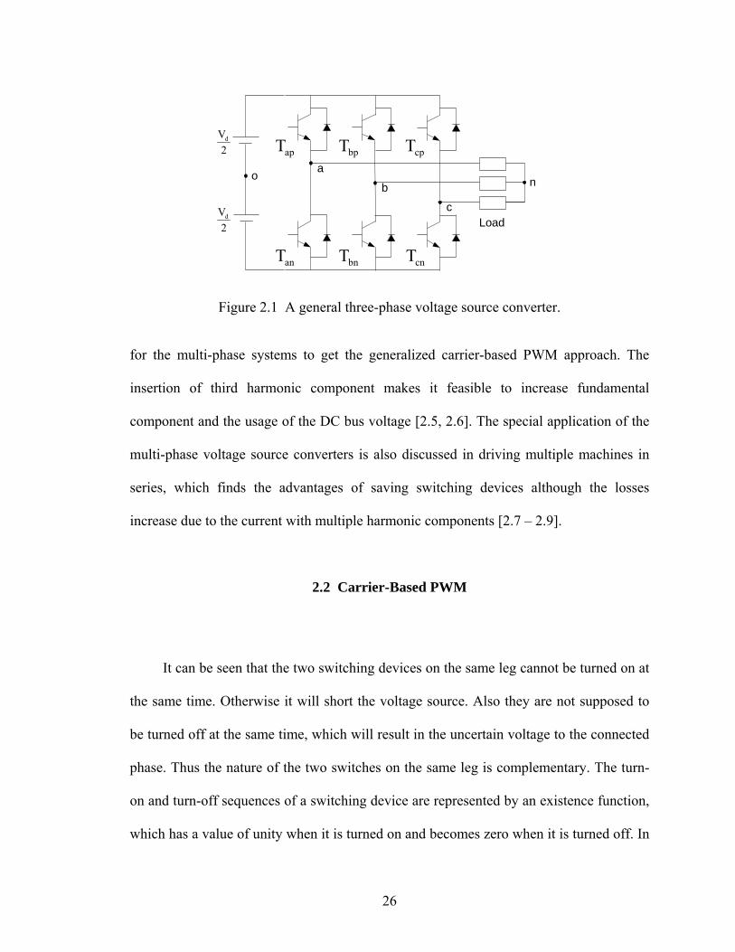
26

Load

nob

a

c

2Vd

2Vd

apT bpT cpT

cnTbnTanT

Figure 2.1 A general three-phase voltage source converter.

for the multi-phase systems to get the generalized carrier-based PWM approach. The

insertion of third harmonic component makes it feasible to increase fundamental

component and the usage of the DC bus voltage [2.5, 2.6]. The special application of the

multi-phase voltage source converters is also discussed in driving multiple machines in

series, which finds the advantages of saving switching devices although the losses

increase due to the current with multiple harmonic components [2.7 – 2.9].

2.2 Carrier-Based PWM

It can be seen that the two switching devices on the same leg cannot be turned on at

the same time. Otherwise it will short the voltage source. Also they are not supposed to

be turned off at the same time, which will result in the uncertain voltage to the connected

phase. Thus the nature of the two switches on the same leg is complementary. The turn-

on and turn-off sequences of a switching device are represented by an existence function,

which has a value of unity when it is turned on and becomes zero when it is turned off. In

27

general, an existence function of a two-level converter comprising of switching devices

Tij is represented by Sij , i = a,b,c and j = p, n where i represents the load phase to which

the device is connected, and j signifies top (p) and bottom (n) device of the inverter leg.

Hence, Sap, San which take values of zero or unity, are, respectively, the existence

functions of the top device (Tap) and bottom device (Tan) of the inverter leg which is

connected to phase ‘a’ load.

1

1

1

=+

=+

=+

cncp

bnbp

anap

SS

SS

SS

(2.1)

In the ideal case, the voltage drop across the switch is immediately zero when the

switch is turned on and the current flowing through the switch is zero when the switch is

turned off. So at any time, the output voltage from the VSI can be expressed as

( )

( )

( ) nocncncpd

nobnbnbpd

noananapd

VVSSV

VVSSV

VVSSV

+=−

+=−

+=−

2

2

2

(2.2)

Since the switching functions for the two switching devices are dependent, it is

convenient to use only one switching function to represent the switching status of each

leg, which is always chosen as the switching function of upper device. So the turn-on and

turn-off actions of the switches produce series of rectangular waveform and the ratio

between the on-duration and a full cycle is defined as duty cycle, which is varying

between 0 and 1. It is thus evident that varying the duty cycle of the switching device will

result into variable output voltage. Both fundamental component and harmonic

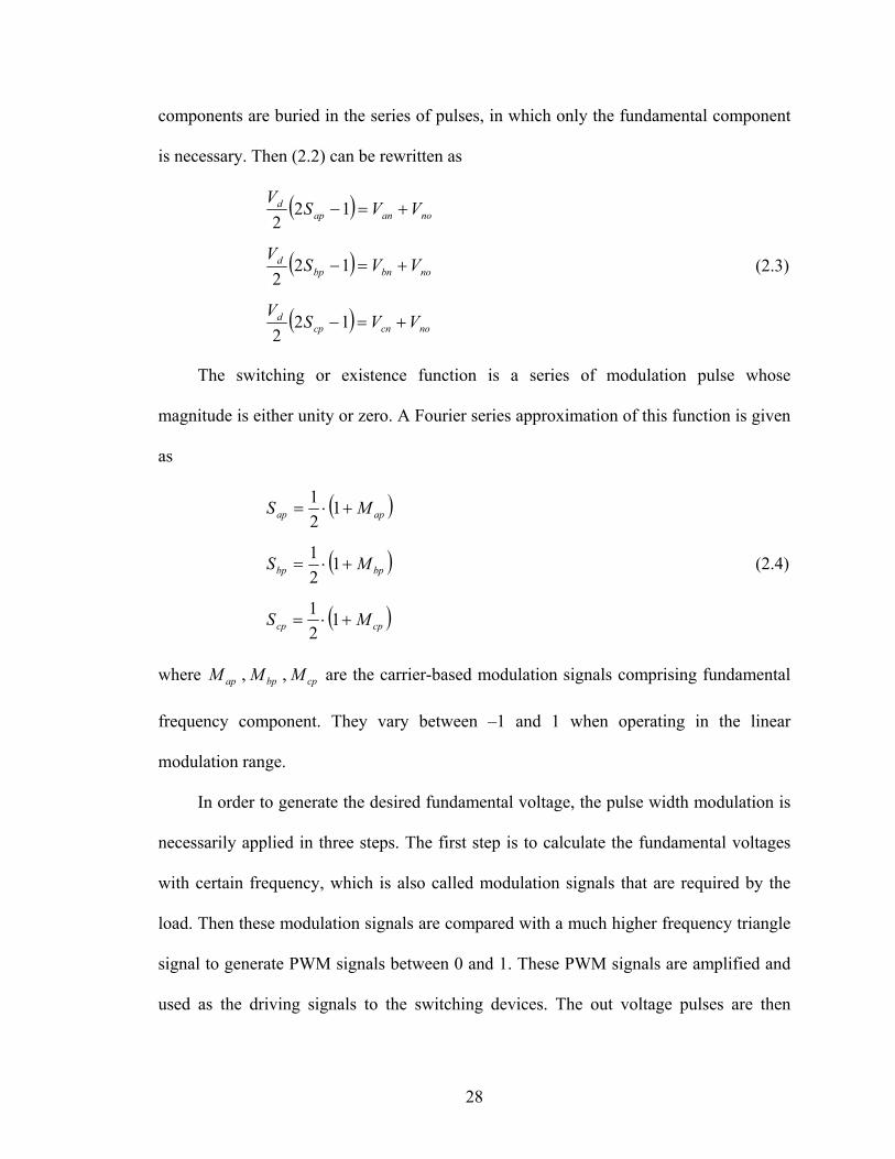
28

components are buried in the series of pulses, in which only the fundamental component

is necessary. Then (2.2) can be rewritten as

( )

( )

( ) nocncpd

nobnbpd

noanapd

VVSV

VVSV

VVSV

+=−

+=−

+=−

122

122

122

(2.3)

The switching or existence function is a series of modulation pulse whose

magnitude is either unity or zero. A Fourier series approximation of this function is given

as

( )

( )

( )cpcp

bpbp

apap

MS

MS

MS

+⋅=

+⋅=

+⋅=

121

121

121

(2.4)

where cpbpap MMM , , are the carrier-based modulation signals comprising fundamental

frequency component. They vary between –1 and 1 when operating in the linear

modulation range.

In order to generate the desired fundamental voltage, the pulse width modulation is

necessarily applied in three steps. The first step is to calculate the fundamental voltages

with certain frequency, which is also called modulation signals that are required by the

load. Then these modulation signals are compared with a much higher frequency triangle

signal to generate PWM signals between 0 and 1. These PWM signals are amplified and

used as the driving signals to the switching devices. The out voltage pulses are then

29

applied to the load, which result in a nearly sinusoidal current when the load is inductive

in most cases. For a three-phase voltage source converter, there are three reference

signals that are compared with the same carrier signal, which is generally a high

frequency triangle wave. The ratio between the magnitude of the reference signal and half

of the DC bus voltage is defined as the modulation index.

2

*

dVVM = (2.5)

The carrier-based PWM using sine-triangle comparison is illustrated in Figure 2.2,

in which the sinusoidal modulation signal is compared with the high frequency triangle

carrier signal. When the modulation signal is greater than the triangle carrier signal, the

output signal is high, which is used to drive the upper device of the phase to be ON state.

The corresponding lower device is then off and the phase is connected to the positive rail

of the DC bus. Whenever the modulation signal is less than the triangle carrier signal, the

output signal is low, which is used to drive the lower device of the phase to be ON state.

The corresponding upper device is then off and the phase is shorted to the negative rail of

the DC bus. Assuming the frequency of the triangle signal is high enough, the

fundamental component that can be extracted from the voltage pulses is almost equal to

the reference signal. The output voltage is linear to the reference signal until the

magnitude of the reference signal reaches Vdc/2, which is the maximum fundamental

voltage that can be achieved. The maximum fundamental voltage that is generated from

six-step operation is ( ) dcVπ/2 . The linear operation range is limited to 78.5 percent. This

limit is overcome by the alternative technique known as space vector modulation.

30

Figure 2.2 Illustration of carrier-based PWM using sine-triangle comparison method. (a)

Modulation signal and carrier (triangle) signal. (b) the switching signal after the

comparison.

The modulation signal generated from TI TMS320LF2407 DSP evaluation board is

shown in Figure 2.3, in which the phase and line to line voltages are also shown.

1

(b)

0

1

(a) 0

-1

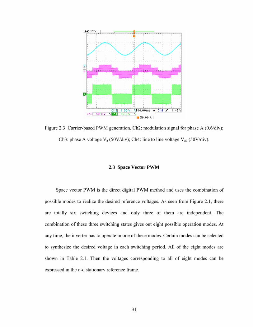
31

Figure 2.3 Carrier-based PWM generation. Ch2: modulation signal for phase A (0.6/div);

Ch3: phase A voltage Va (50V/div); Ch4: line to line voltage Vab (50V/div).

2.3 Space Vector PWM

Space vector PWM is the direct digital PWM method and uses the combination of

possible modes to realize the desired reference voltages. As seen from Figure 2.1, there

are totally six switching devices and only three of them are independent. The

combination of these three switching states gives out eight possible operation modes. At

any time, the inverter has to operate in one of these modes. Certain modes can be selected

to synthesize the desired voltage in each switching period. All of the eight modes are

shown in Table 2.1. Then the voltages corresponding to all of eight modes can be

expressed in the q-d stationary reference frame.

32

For the three-wire system as shown in Figure 2.1, the sum of three phase voltages is

zero. Then the voltage between the load neutral and the reference point of DC voltage is

determined from (2.3).

( )

⎟⎠⎞

⎜⎝⎛ −++=

=−++

23

3

332222

cpbpapd

no

nocpbpapd

SSSV

V

VSSSV

(2.6)

After substituting the above voltage into (2.3) again, the phase voltages can be

expressed in terms of three switching functions and the DC bus voltage.

( )

( )

( )cpbpapd

cp

cpbpapd

bp

cpbpapd

ap

SSSV

V

SSSV

V

SSSV

V

23

23

23

+−−=

−+−=

−−=

(2.7)

The general transformation between different reference frame (abc stationary

reference frame and q-d reference frame) is illustrated in Figure 2.4, in which 'f'

represents any quantity in the certain frame including the voltage, current, flux linkage

etc. And the corresponding transformation matrix (both the transformation and the

inverse transformation) is shown in (2.8) assuming the angle between these two reference

frames is θ .

33

(q-axis)

(d-axis)bf

( )sqa ff

cf

θ

ω

sdf

df

qf

Figure 2.4 Transformation between reference frames.

⎥⎥⎥

⎦

⎤

⎢⎢⎢

⎣

⎡

⎥⎥⎥⎥⎥⎥⎥

⎦

⎤

⎢⎢⎢⎢⎢⎢⎢

⎣

⎡

⎟⎠⎞

⎜⎝⎛ +⎟

⎠⎞

⎜⎝⎛ +

⎟⎠⎞

⎜⎝⎛ −⎟

⎠⎞

⎜⎝⎛ −=

⎥⎥⎥

⎦

⎤

⎢⎢⎢

⎣

⎡

⎥⎥⎥

⎦

⎤

⎢⎢⎢

⎣

⎡

⎥⎥⎥⎥⎥⎥⎥

⎦

⎤

⎢⎢⎢⎢⎢⎢⎢

⎣

⎡

⎟⎠⎞

⎜⎝⎛ +⎟

⎠⎞

⎜⎝⎛ −

⎟⎠⎞

⎜⎝⎛ +⎟

⎠⎞

⎜⎝⎛ −

=⎥⎥⎥

⎦

⎤

⎢⎢⎢

⎣

⎡

0

0

13

2sin3

2cos

13

2sin3

2cos

1sincos

21

21

21

32sin

32sinsin

32cos

32coscos

32

fff

fff

fff

fff

d

q

c

b

a

c

b

a

d

q

πθπθ

πθπθ

θθ

πθπθθ

πθπθθ

(2.8)

In the space vector PWM, the transformation between abc and stationary q-d

reference frames is needed just for the voltages. Then the voltages in q-d reference frame

are calculated for all eight modes using (2.9) assuming the sum of three-phase voltages is

zero. The voltage between the load neutral and the reference point of DC voltage is

calculated from (2.6).

34

( )

( )

( )

⎟⎠⎞

⎜⎝⎛ −++=

+−=

+−=

−−==

23

3

31

31

23

cpbpapd

pn

cpbp

cnbndp

cpbpapd

anqp

SSSV

V

SS

VVV

SSSV

VV

(2.9)

Table 2.1 Switching modes of the three-phase voltage source inverter and corresponding

stationary reference frame qdns voltages

Mode Sap Sbp Scp Vqp Vdp Vpn

U0 0 0 0 0 0 -2dV

U5 0 0 1 -3dV

3dV

-6dV

U3 0 1 0 -3dV

-3dV

-6dV

U4 0 1 1 -3

2 dV 0

6dV

U1 1 0 0 3

2 dV 0 -

6dV

U6 1 0 1 3dV

3dV

6dV

U2 1 1 0 3dV

-3dV

6dV

U7 1 1 1 0 0 2dV

35

These modes and corresponding q-d-o voltages are shown in Figure 2.5, which is

also called as the space vector diagram.

In order to synthesize the desired three-phase voltages, these voltages are

transformed into the stationary reference frame as Vqd* as shown in Figure 2.5. The

general transformation for any three-phase voltage set is

⎟⎠⎞

⎜⎝⎛ ++=

⎟⎟⎠

⎞⎜⎜⎝

⎛+−=

⎟⎠⎞

⎜⎝⎛ −−=

cnbnanos

cnbnds

cnbnanqs

VVVV

VVV

VVVV

21

21

21

32

23

23

32

21

21

32

*

*

*

(2.10)

Im

Re

U1 (110)U2 (010)

U0(000) U6 (100)

U4 (001)

U3 (011)

U5 (101)

U7(111)

⎥⎦

⎤⎢⎣

⎡ −6

,0,3

2 dd VV

⎥⎦

⎤⎢⎣

⎡ −633ddd V,V,V

⎥⎦⎤

⎢⎣⎡ −−−

6,

3,

3ddd VVV

⎥⎦⎤

⎢⎣⎡−

60

32 dd V,,V

⎥⎦

⎤⎢⎣

⎡−−

6,

3,

3ddd VVV

⎥⎦

⎤⎢⎣

⎡6

,3

,3

ddd VVV

at

bt *qdV

⎥⎦⎤

⎢⎣⎡ −

2,0,0 dV

⎥⎦⎤

⎢⎣⎡

2,0,0 dV

Figure 2.5 Voltage space vector diagram for three-leg, three-phase voltage source

converter including zero sequence voltages.

36

For the balanced case, Vos* is equal to zero. However, in general

noospn VVV += * (2.11)

This reference voltage vector is then used to calculate the turn-on times of the

inverter switching devices required to synthesize a reference three-phase balanced

voltage set. In general, the three-phase balanced voltages expressed in the stationary

reference frame, situated in the appropriate sector in Figure 2.5, are approximated by the

time-average over a sampling period (inverter switching period, Ts) of the two adjacent

active q-d voltage vectors and the two zero states U0 and U7 in order to minimize the

number of switching during transient. If the normalized times (with respect to modulator

sampling time or inverter switching period, Ts) of the four voltage vectors termed as Vqda

, Vqdb, Vqd0, Vqd7 are ta , tb, t0, t7 respectively. The q and d components of the reference

voltage Vqd* and the zero sequence voltage are approximated as

7700*

7700*

7700*

tVtVtVtVVV

tVtVtVtVV

tVtVtVtVV

pnpnbpnbapnaosno

dpdpbdpbadpads

qpqpbqpbaqpaqs

+++>=+<

+++=

+++=

(2.12)

where Vos is the zero sequence voltage due to the three-phase reference voltages. It is

observed that both Vqd0 and Vqd7 do not influence the values of ta and tb .

⎥⎦

⎤⎢⎣

⎡⎥⎦

⎤⎢⎣

⎡=⎥

⎦

⎤⎢⎣

⎡

b

a

dpbdpa

qpbqpa

ds

qs

tt

VVVV

VV

*

*

(2.13)

So the times for the two active states are calculated as

⎥⎦

⎤⎢⎣

⎡⎥⎦

⎤⎢⎣

⎡=⎥

⎦

⎤⎢⎣

⎡−

*

*1

ds

qs

dpbdpa

qpbqpa

b

a

VV

VVVV

tt

37

dpaqpbdpbqpa

dsqpaqsdpab

dpaqpbdpbqpa

dsqpbqsdpba

VVVVVVVV

t

VVVVVVVV

t

−⋅+⋅−

=

−⋅−⋅

=

**

**

(2.14)

In general, the sum of these two times is less than 1 when the inverter works in the

linear modulation region. Hence the time left has to be utilized by the two null states.

( ) c

c

bac

tt

tt

ttt

⋅−=

⋅=

−−=

α

α

1

1

7

0 (2.15)

where 10 ≤≤α . In general, it has been shown that the best voltage synthesis is achieved

when the converter is operating in the linear modulation region when α = 0.5.

One of the most frequently used sequences to synthesize a reference voltage vector

that is rotating counter-clockwise for all six sectors is shown in Figure 2.6. In each sector,

the starting and ending conditions for all upper switching devices are state mode 0 while

the state mode 7 happens in the middle of the switching period. The minimum switching

is achieved by this arrangement.

The modulation signal generated from DSP is shown in Figure 2.7, in which the

reference phase voltage, phase, and line to line voltages are also shown.

38

apS

apS

bpS

cpS

bpS

cpS

apS

bpS

cpS

Sector: I

Sector: III

Sector: II

2t0

2t7

2tb

2ta

2t7

2t0

2tb

2ta

2t0

2t7

2tb

2ta

2t7

2t0

2tb

2ta

2t0

2t7

2tb

2ta

2t7

2t0

2tb

2ta

2Ts

2Ts

Figure 2.6a Existence functions of top devices in sectors I, II, III.

39

apS

bpS

cpS

apS

apS

bpS

cpS

bpS

cpS

Sector: V

Sector: IV

Sector: VI

2Ts

2Ts

2t0

2t7

2tb

2ta

2t7

2t0

2tb

2ta

2t0

2t7

2tb

2ta

2t7

2t0

2tb

2ta

2t0

2t7

2tb

2ta

2t7

2t0

2tb

2ta

Figure 2.6b Existence functions of top devices in sectors IV, V, VI.

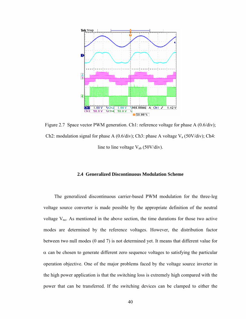
40

Figure 2.7 Space vector PWM generation. Ch1: reference voltage for phase A (0.6/div);

Ch2: modulation signal for phase A (0.6/div); Ch3: phase A voltage Va (50V/div); Ch4:

line to line voltage Vab (50V/div).

2.4 Generalized Discontinuous Modulation Scheme

The generalized discontinuous carrier-based PWM modulation for the three-leg

voltage source converter is made possible by the appropriate definition of the neutral

voltage Vno. As mentioned in the above section, the time durations for those two active

modes are determined by the reference voltages. However, the distribution factor

between two null modes (0 and 7) is not determined yet. It means that different value for

α can be chosen to generate different zero sequence voltages to satisfying the particular

operation objective. One of the major problems faced by the voltage source inverter in

the high power application is that the switching loss is extremely high compared with the

power that can be transferred. If the switching devices can be clamped to either the

41

positive or negative rails of the DC link voltage during some switching periods, the

effective switching frequency will reduce and the switching loss will also decrease. But

the line-line voltages remain the same. This is so-called discontinuous PWM and there

are different types of discontinuous PWM schemes. Since all of these different schemes

are based on the selection of α, it is possible to derive the general expression that is used

to generate all the possibilities.

The average neutral voltage, Vno, can be determined using the method of space

vector modulation and the voltages of the three-phase voltage source converter. As seen

from (2.10), the zero sequence voltage is determined by the selection of α since ta and tb

are calculated from the desired balance reference voltages. For example, in sector I, the

switching times for the two active modes are calculated as

dqpa VV32

= , 0=dpaV ; dqpb VV31

= , ddpb VV3

1−=

Im

Re

Ub (110)

Ua (100)

⎥⎦

⎤⎢⎣

⎡−

6,0,

32 dd VV

⎥⎦⎤

⎢⎣⎡ −

633ddd V,V,V

at

bt *qdV

Figure 2.8 Time determination in sector I.

42

d

ds

dpaqpbdpbqpa

dsqpaqsdpab

d

dsqs

dpaqpbdpbqpa

dsqpbqsdpba

VV

VVVVVVVV

t

VVV

VVVVVVVV

t

***

****

3

233

−=

−

⋅+⋅−=

+=

−

⋅−⋅=

(2.16)

Similarly the times in other sectors can be calculated as shown in Table 2.2.

Then these times can be further expressed in terms of reference phase voltages and

even the line-line voltages in Table 2.3 using the inverse transformation.

osdsqscn

osdsqsbn

osqsan

VVVV

VVVV

VVV

++−=

+−−=

+=

23

21

23

21 (2.17)

Table 2.2 Device Switching times expressed in terms of reference voltages

Sector I II III

at d

dsqs

VVV

233 ** +

d

dsqs

VVV

233 ** −

d

ds

VV *3−

bt d

ds

VV *3−

d

dsqs

VVV

233 ** −−

d

dsqs

VVV

233 ** +−

Sector IV V VI

at d

dsqs

VVV

233 ** −−

d

dsqs

VVV

233 ** +−

d

ds

VV *3

bt d

ds

VV *3

d

dsqs

VVV

233 ** +

d

dsqs

VVV

233 ** −

43

Table 2.3 Device Switching times expressed in terms of reference line-line voltages

Sector I II III IV V VI

at d

ab

VV

d

ac

VV

d

bc

VV

d

ba

VV

d

ca

VV

d

cb

VV

bt d

bc

VV

d

ba

VV

d

ca

VV

d

cb

VV

d

ab

VV

d

ac

VV

Max voltage osap VV − osbp VV − osbp VV − oscp VV − oscp VV − osap VV −

Min voltage oscp VV − oscp VV − osap VV − osap VV − osbp VV − osbp VV −

The average neutral voltage for each sector can be generalized in terms of the

calculated times as shown in Table 2.4.

The general expression for the average neutral voltage can be derived by

considering Tables 2.3 and 2.4 together and expressing the average zero sequence voltage

in terms of the maximum and minimum reference phase voltages. For example, in sector

1,

osap VVV −=max , oscp VVV −=min and ( )minmax VVVV osbp +−=−

dd

aba V

VVVV

t minmax2 +== ,

dd

bcb V

VVVV

t minmax 2−−==

dbac V

VVttt minmax11

−−=−−=

Table 2.4 Average neutral voltage for all sectors

Sectors I, III, V II, IV, VI

>< noV ( ) ( ) cd

abd t

Vtt

Vα21

26−+− ( ) ( ) c

dba

d tV

ttV

α2126

−+−

44

( ) ( )

( )

( ) maxmin

minmaxminmax

)1(212

12122

2126

VVV

VVVVVV

tV

ttV

V

d

d

d

cd

abd

no

ααα

α

α

−−−−=

⎟⎟⎠

⎞⎜⎜⎝

⎛ −−−+

−−=

−+−>=<

(2.18)

After calculating the average zero sequence voltages for all six sectors, the equation

(2.18) becomes the general expression for the average zero sequence voltage. In the case

of carrier-based PWM, this zero sequence voltage is added to the fundamental component

to generate the modulation signal, which is compared with a carrier signal. The final

modulation signal is

( )ddd

ipip V

VVV

VV

M maxmin 2)1(221

2ααα −−−−+= (2.19)

where i = a, b, c representing three phases.

In the implementation of this modulation scheme, the null-state partition parameter

(α) can take any form (constant or time-varying) ranging between 0 and 1. The choice of

α affects the average neutral voltage between the load star-point and the inverter

reference point. In the conventional space vector modulation, α is generally taken as 0.5.

When α is either 0 or 1 and for any depth of modulation magnitude, each switching

device ceases to switch for a total of 120 degrees per fundamental cycle. Under the above

condition, the switching losses and effective inverter switching frequency are

significantly reduced. However, other functions of α may be used, which may lead to

performance improvement of the modulator. The selection of α gives rise to an infinite

number of possible carrier-based PWM modulation signals, some of which have been

45

discovered and referred to as the generalized discontinuous PWM. The generalized

discontinuous modulation signal is obtained when [2.10]:

[ ] )(3cossgn121 δωα ++= t (2.20)

where sgn(X) is 1, 0 and –1 when X is positive, zero, and negative, respectively. By

varying the modulation angle δ, various discontinuous modulation signals are generated.

In general, it has been shown that the best voltage synthesis when the inverter is

operating in the linear modulation region and α = 0.5. In the over-modulation regions, the

generalized discontinuous scheme is most appropriate with a promise of enlarged voltage

linearity, if the appropriate modulation angle δ is utilized.

For the direct implementation (space vector PWM), this is realized by selecting the

appropriate α and calculating the equivalent on-durations for three top switching devices.

Then the existence functions shown in Figure 2.6 are applied when the reference voltage

is located in one of six sectors.

The modulation signals generated from DSP are shown in Figure 2.9, in which the

reference phase voltage, phase and line to line voltages are also shown. By varying δ , the

difference in the modulation signals can be seen clearly in the figures below.

The turn-on times for the three top devices corresponding to the three legs are listed

in Table 2.5. All of these times are within 0 and 1 (normalized with respect to the

switching period). These times can actually be used as the modulation signals. And the

same PWM signals will be generated if the carrier triangle signal is limited within 0 and 1

instead of within –1 and 1, and then used for the comparison as in the above sine-triangle

PWM method.

46

Figure 2.9 Generalized discontinuous PWM generation using

[ ] )(3cossgn15.0 δωα ++⋅= t : (a) o0=δ ; (b) o30−=δ ; (c) o60−=δ . Ch1: reference

voltage for phase A (0.6/div); Ch2: modulation signal for phase A (0.6/div); Ch3: phase

A voltage Va (50V/div); Ch4: line to line voltage Vab (50V/div).

(a)

(b)

(c)

47

Table 2.5 Normalized times when the three top devices are turned on.

Sector I II III IV V VI

apτ 7ttt ba ++ 7tta + 7t 7t 7ttb + 7ttt ba ++

bpτ 7ttb + 7ttt ba ++ 7ttt ba ++ 7tta + 7t 7t

cpτ 7t 7t 7ttb + 7ttt ba ++ 7ttt ba ++ 7tta +

2.5 Modulation Scheme for Multi-Phase Systems

In all multi-phase electric machines, multi-phase converters are required to deliver

currents of different frequencies either for use of single machines requiring fundamental

and third harmonic currents to improve torque capability or to achieve independent

control of serially connected motors needing many fundamental frequency currents for

the mutually decoupled machines. Traditionally, the multi-phase converters use

hysteresis-type current controllers to impress the required currents. Although very simple

to implement, its inherent nonlinearity, the varying switching frequency of the converters

lead to uneven distribution of losses in the switching devices of the converter. This then

constrains the converter thermal design and selection of converter filtering elements.

Hence it is not the optimum control scheme for high power applications where efficiency

optimization and ease of converter cooling are premium design requirements. It is

desirable therefore to use control schemes that ensure defined converter switching

frequency such as the space vector PWM and carrier-based sine-triangle PWM

modulation to command the load phase voltages that impress the commanded multi-

frequency (non-sinusoidal) phase currents. The feasibility of controlling individual

48

components of the non-sinusoidal phase currents of multi-phase motors using

synchronous reference frame current controllers and voltage source converters has been

established. Each current component in their individual synchronous reference frames

yields constant dc qd quantities which with the classical PI controllers and decoupling

schemes can be regulated without phase and magnitude errors [2.16]. The outputs of the

controllers are commanded phase voltages for each frequency component which are used

to synthesize the converter output voltages.

While existing multi-motor drives use a common dc bus to drive converters, each

feeding a three-phase motor which are individually and independent controlled. The

multi-phase machines provide the opportunity that two or more machines can be

connected in series by using single inverter. It is envisaged that multiphase machines with

other serially connected motors fed with single multi-phase converters will deliver the

advantages of few converter legs and associated control circuitry without comprising the

independent controllability of the individual drives.

This section presents the generalized carrier-based continuous and discontinuous

PWM techniques to generate all the possible voltage components of multiphase

converters with special attention paid to the five and six phase variants. Carrier-based

sine-triangle modulation scheme is preferred in multiphase converters when compared to

the digitally implemented space vector because of its simplicity of implementation either

digitally or analogically (it requires calculation of switching times and sequencing of the

switching states). With the proposed modulation, it is possible with a single five phase

converter to drive a five phase machine connected in series with another five-phase

machine with a transposed winding arrangement which are independently controlled

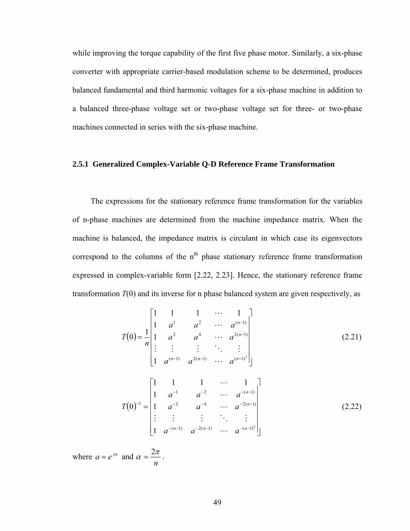
49

while improving the torque capability of the first five phase motor. Similarly, a six-phase

converter with appropriate carrier-based modulation scheme to be determined, produces

balanced fundamental and third harmonic voltages for a six-phase machine in addition to

a balanced three-phase voltage set or two-phase voltage set for three- or two-phase

machines connected in series with the six-phase machine.

2.5.1 Generalized Complex-Variable Q-D Reference Frame Transformation

The expressions for the stationary reference frame transformation for the variables

of n-phase machines are determined from the machine impedance matrix. When the

machine is balanced, the impedance matrix is circulant in which case its eigenvectors

correspond to the columns of the nth phase stationary reference frame transformation

expressed in complex-variable form [2.22, 2.23]. Hence, the stationary reference frame

transformation T(0) and its inverse for n phase balanced system are given respectively, as

( )

⎥⎥⎥⎥⎥⎥

⎦

⎤

⎢⎢⎢⎢⎢⎢

⎣

⎡

=

−−−

−

−

2)1()1(2)1(

)1(242

)1(21

1

11

1111

10

nnn

n

n

aaa

aaaaaa

nT

L

MOMMM

L

L

L

(2.21)

( )

⎥⎥⎥⎥⎥⎥

⎦

⎤

⎢⎢⎢⎢⎢⎢

⎣

⎡

=

−−−−−−

−−−−

−−−−

−

2)1()1(2)1(

)1(242

)1(21

1

1

11

1111

0

nnn

n

n

aaa

aaaaaa

T

L

MOMMM

L

L

L

(2.22)

where αjea = and nπα 2

= .

50

For five phase balanced variables edcba fffff , , , , , the generalized qd arbitrary

reference frame transformed variables expressed in the complex-variable form are

[ ]edcba ffffff 5/10 ++++= (2.23a)

[ ] 14321 5/1 ej

edcbaqd efafafaafff ϕ−++++=

(2.23b)

[ ] 23422 5/1 ej

edcbaqd efafafafaff ϕ−++++=

(2.23c)

[ ] 32433 5/1 ej

edcbaqd efafaaffaff ϕ−++++=

(2.23d)

[ ] 4 5/1 2344

ejedcbaqd eaffafafaff ϕ−++++=

(2.23e)

For the six-phase balanced variables, fedcba ffffff , , , , , , the generalized qd

arbitrary reference frame transformed variables expressed in the complex-variable form

are

[ ]fedcba fffffff 6/10 +++++= (2.24a)

[ ] 154321 6/1 ej

fedcbaqd efafafafaafff ϕ−+++++= (2.24b)

[ ] 242422 6/1 ej

fedcbaqd efafaffafaff ϕ−+++++= (2.24c)

[ ] 33333 6/1 ej

fedcbaqd efaffaffaff ϕ−+++++= (2.24d)

[ ] 424244 6/1 ej

fedcbaqd efafaffafaff ϕ−+++++= (2.24e)

[ ] 523455 6/1 ej

fedcbaqd eaffafafafaff ϕ−+++++= (2.24f)

n1,2,i , L=+= ieiei t ϕωϕ , eiω are the rotating frequencies of the reference frames and

the initial angles are iϕ .

51

Multi-phase motor windings produce a torque-producing rotating field only if the

spatial displacement angles of its phase windings are equal to the temporal displacement

angles of the phase currents. The transformed quantities comprise of zero, positive and

negative sequence components of which only the positive and negative sequence

components produce average torque. Hence, the positive, negative and zero sequence

motor magnetomotive force (MMF) can be determined by transforming the MMFs

produced by the phases using (2.23-24) for five and six phase machines. It is assumed

that the fundamental components of the n-phase machine winding functions are mutually

displaced by 2π/n in the positive sequence and the phase currents are also spatially

displaced by the same angle, but sequenced in all possible orders. For the five phase

machine, (2.23a) gives the zero sequence component, two positive sequences are

produced by (2.23b-23c) and negative sequence MMFs are also produced by (2.23d-23e).

Hence, the windings producing the two positive sequence MMFs can be connected as

shown in Figure 2.10. For the third harmonic MMF of the windings, a positive sequence

MMF is produced only with the use of 2.23(b). From this analysis and Figure 2.10, it is

inferred that average torques can be produced with the serial connection of two five-

phase winding machines with phase current transposition in the second machine. A

balanced third harmonic current in the first machine will also produce an average torque

interacting with its third harmonic MMF. Hence the five-phase converter feeding the

machine must generate up to three voltage components. Similar considerations lead to

Figure 2.11 for the six-phase machines. The feasible serial connections shown in Figure

2.11 consist of a six-phase and a three-phase machine for which the six-phase converter

delivers possible two voltage components for the two machines.

52

aI

bI

cI

dI

eI

1a

1b

1c

1d

1e

2a

2b

2c

2d

2e

Figure 2.10 Feasible windings connections for five-phase machines : series connection

of machines.

1a

1b

1c

1d

1e

2a

2b

2c

1f

Figure 2.11 Feasible windings connections for six-phase machines : series connection of

machines, six and three-phase machines.

2.5.2 Modulation Technique for Multi-Phase Converters

Figure 2.12 shows a schematic diagram of a multi-phase voltage source converter.

The switching of the devices are described by switching functions which take values of

one and zero when the devices are turned on or turned off, respectively.

53

apT bpT npT

anT bnT nnT

ab

n

2dV

o

aEaLar+ -

aIbEbL

br+ -

nEnLnr

+ -

bI

nI

2dV

n

Figure 2.12 Schematic diagram of a multi-phase voltage source converter.

The switching functions of the top devices are ipS (i = a, b, c, … ,n) are

complimentary with the switching functions of the bottom devices. The n-phase voltages

are therefore expressed as

( ) noinipd VVS

V+=−⋅ 12

2,

( )ipip MS +⋅= 121 , nedcbai ,,,,,, L= (2.25)

ipS and ipM are the switching functions and the modulation signals for the ith leg,

respectively. The neutral voltage is noV and the phase voltages are inV . The expression for

the modulation signals which are compared with a high frequency triangle waveform

using sine-triangle carrier-based PWM technique to synthesize the desired phase voltages

inV (which may be multi-frequency, in general) is given as

2/d

noinip V

VVM

+= (2.26)

54

The neutral voltage noV in (2.25) is indeterminate and can take any realistic values.

When noV is set equal to zero or is a continuous function of time, continuous modulation

signals and a continuous carrier-based modulation scheme result. However the

performance of the converter can be enhanced with the selection of an appropriate

expression of the average neutral sequence voltage like it is done in three-phase, two

level converters to achieve discontinuous, continuous, and space vector carrier-based

PWM modulation [2.10, 2.24]. In this section, the stationary reference frame transformed

converter phase voltages are used to determine the expression for the average neutral

voltage which substituted in (2.26) yields the equation for the modulation signals.

2.5.3 Modulation for Five-Phase Converters

A five-phase voltage source converter with an input DC voltage given as dV has 32

switching modes, 30 of which are active and the other two are null modes. The converter

is to generate the five phase voltages ( anV , bnV , cnV , dnV , enV ) comprising of sum of all or

some of the voltage sets ( 1anV , 1bnV , 1cnV , 1dnV , 1enV ), ( 2anV , 2bnV , 2cnV , 2dnV , 2enV ) and

( 13anV , 13bnV , 13cnV , 13dnV , 13enV ) expressed as ( 5/2πα = ):

( )( )

( )

( )( )αγω

αγω

αγω

αγω

γω

4cos

3cos

2cos

cos

cos

11

11

11

11

11

−+=

−+=

−+=

−+=

+=

tVV

tVV

tVV

tVV

tVV

een

edn

ecn

ebn

ean

(2.27a)

55

( )( )

( )

( )( )αβω

αβω

αβω

αβω

βω

43cos

33cos

23cos

3cos

3cos

1313

1313

1313

1313

1313

−+=

−+=

−+=

−+=

+=

tVV

tVV

tVV

tVV

tVV

een

edn

ecn

ebn

ean

(2.27b)

( )( )

( )

( )( )αξω

αξω

αξω

αξω

ξω

3cos

cos

4cos

2cos

cos

222

222

222

222

222

−+=

−+=

−+=

−+=

+=

tVV

tVV

tVV

tVV

tVV

en

dn

cn

bn

an

(2.27c)

The phase angles of the voltages are ξ, γ, β. The phase and neutral voltages from

(2.25) for the five-phase converter are

( )25

2

2

2

2

2

depdpcpbpap

dno

noend

epd

nodnd

dpd

nocnd

cpd

nobnd

bpd

noand

apd

VSSSSS

VV

VVV

SV

VVV

SV

VVV

SV

VVV

SV

VVV

SV

−++++=

+=−

+=−

+=−

+=−

+=−

(2.28)

Hence, for balanced phase voltages, the converter phase and neutral voltages are

given as

56

( )

( )

( )

( )

( )epdpcpbpapd

en

epdpcpbpapd

dn

epdpcpbpapd

cn

epdpcpbpapd

bn

epdpcpbpapd

an

SSSSSV

V

SSSSSV

V

SSSSSV

V

SSSSSV

V

SSSSSV

V

45

45

45

45

45

+−−−−=

−+−−−=

−−+−−=

−−−+−=

−−−−=

(2.29)

Substituting (2.29) into (2.23), the stationary reference frame qd voltages for each

of the four components are calculated and displayed in Figure 2.13. It is however,

observed that space vectors 1qdV and 4qdV are complex conjugates, so are 2qdV and 3qdV .

Hence, only two space vectors 1qdV and 2qdV are used for voltage synthesis. 1qdV

generates the fundamental frequency voltages (2.27a) and 2qdV produces the third

harmonic voltages (2.27b) required for the third harmonic machine MMF for torque

production or voltages in (2.27c) to interact with the transposed second five phase

machine connected with the first machine. The voltage vectors of the neutral voltage oV

are used for the determination of the average neutral voltage required in (2.26).

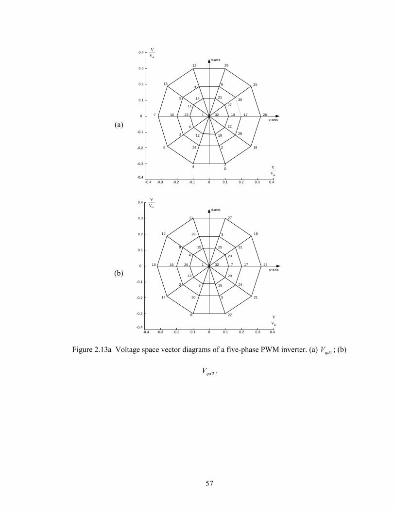
57

q-axis

d-axis29

204

8

7

15

13

16 17

30

26

25

24

28

182

5

931

226

1023

11 27

2114

3 1912

1 32

0-0.3

-0.2

-0.4-0.4

-0.3

-0.2 -0.1 0.1 0.2 0.3 0.4

-0.1

0

0.1

0.2

0.3

0.4dcV

V

dcVV

q-axis

d-axis

29

204

8

7

15

13

16 17

30

26

25

24

28

182

5

9 31

226

10 23

11 27

2114

3 1912

1 32

0-0.3

-0.2

-0.4-0.4

-0.3

-0.2 -0.1 0.1 0.2 0.3 0.4

-0.1

0

0.1

0.2

0.3

0.4dcV

V

dcVV

Figure 2.13a Voltage space vector diagrams of a five-phase PWM inverter. (a) 1qdV ; (b)

2qdV .

(a)

(b)

58

q-axis

d-axis

29

204

8

7

15

13

16 17

30

26

25

24

28

182

5

9 31

22

6

10 23

11

27

2114

3 1912

1 32

0-0.3

-0.2

-0.4-0.4

-0.3

-0.2 -0.1 0.1 0.2 0.3 0.4

-0.1

0

0.1

0.2

0.3

0.4dcV

V

dcVV

q-axis

d-axis

29

204

8

7

15

13

16 17

30

26

25

24

28

182

5

931

226

1023

11 27

2114

3 1912

1 32

0-0.3

-0.2

-0.4-0.4

-0.3

-0.2 -0.1 0.1 0.2 0.3 0.4

-0.1

0

0.1

0.2

0.3

0.4dcV

V

dcVV

0.30.1 0.5-0.5 -0.3 -0.1

A B DC E F

1A = 2,3,5,9,17B = 25,21,19,18,13,11,10,7,6,4C =

29,27,26,23,22,20,15,14,12,8D = 31,30,28,24,16E = 32F =

dcVV

Figure 2.13b Voltage space vector diagrams of a five-phase PWM inverter. (a) 3qdV ; (b)

4qdV ; (c) oV .

(a)

(b)

(c)

59

Vectors with the largest values in 1qdV give the least magnitude voltages in 2qdV ,

while the middle valued vectors in 1qdV are corresponding to the middle valued vectors in

2qdV . Active vectors used to synthesize voltages are chosen as the outer and middle

vectors in 1qdV as shown in Figure 2.14.

Reference voltages *1qdV and *

2qdV in any sector of the space vector are synthesized

by time-averaging some four active and two null voltage vectors as illustrated in Figure

2.14 for sector 1. In sector 1 of the 1qdV space vector, the active modes are [17( 11qdV ),

25( 14qdV ), 26( 12qdV ), 30( 13qdV )] and the two null vectors are [1( 101qdV ) and 32( 132qdV )].

The corresponding voltage vectors in 2qdV are also selected. Since the qd voltages of the

null vectors are zero, the linear equations for determining the averaging times for the

vectors are

032232012014243232221212

032132011014143132121111

tVtVtVtVtVtVV

tVtVtVtVtVtVV

qdqdqdqdqdqdqd

qdqdqdqdqdqdqd

+++++=

+++++= (2.30)

q-axis

d-axis

17

30

26

25

10

27*

qdV

1Vv

4Vv

3Vv

2Vv

1,32

Figure 2.14 Synthesis of the fundamental voltage in sector 1.

60

The time ratio between two null states (1 and 32) are defined as ctt µ=01 ,

( ) ctt µ−= 1032 with the variable µ ranging between zero and unity. With

( )43211 tttttc +++−= , the average neutral voltage corresponding to the selected voltage

vectors for sector 1 is

( ) ( ) ( )

( )( )

( )

( )

( )4321

422

311

4321

4231

5254

2156

2156

52

54

2

ttttV

ttV

ttV

tttt

ttttV

V

oo

o

o

do

+++=

−=

+−=

⎥⎦⎤+++−−

⎢⎣⎡ −+−++−=

µ

µ

(2.31)

The expressions for times t1, t2, t3, and t4 obtained from (2.30) are substituted into

(2.31) yielding the neutral sequence voltage in terms of 1qdV and 2qdV . Calculations

similar to (2.30-31) are done for all the ten sectors of 1qdV for which ten expressions are

obtained for the average neutral voltages. Using the inverse stationary reference frame

transformations (2.22) the qd voltages in the equations for the ten average neutral

voltages are expressed in terms of the phase voltages ( anV , bnV , cnV , dnV , enV ). It is

further desirable to reduce the complexity of these expressions and unify them by

expressing them in terms of the instantaneous maximum and minimum phase voltages

maxV , minV . When the q- and d-axis reference voltages are expressed in terms of phase

voltages, the times spent on the voltage vectors can be calculated. The coefficients of the

phase voltages are shown in Table 2.6, which is corresponding to the condition when Vqd2

= 0.

61

Table 2.6a Analysis on Vo1 for Vqd1 (Vqd2 = 0)

Sector -0.2211 0.5789 0.5789 -0.2211 -0.7155

1 Va Vb Vc Vd Ve

2 Vb Va Ve Vd Vc

3 Vb Vc Vd Ve Va

4 Vc Vb Va Ve Vd

5 Vc Vd Ve Va Vb

6 Vd Vc Vb Va Ve

7 Vd Ve Va Vb Vc

8 Ve Vd Vc Vb Va

9 Ve Va Vb Vc Vd

10 Va Ve Vd Vc Vb

Table 2.6b Analysis on Vo2 for Vqd1 (Vqd2 = 0)

Sector 0.1789 -0.4683 -0.4683 0.1789 0.5789

1 Va Vb Vc Vd Ve

2 Vb Va Ve Vd Vc

3 Vb Vc Vd Ve Va

4 Vc Vb Va Ve Vd

5 Vc Vd Ve Va Vb

6 Vd Vc Vb Va Ve

7 Vd Ve Va Vb Vc

8 Ve Vd Vc Vb Va

9 Ve Va Vb Vc Vd

10 Va Ve Vd Vc Vb

62

Table 2.6c Analysis on Voo for Vqd1 (Vqd2 = 0)

Sector 0.7236 0.4472 -0.4472 -0.7236 0

1 Va Vb Vc Vd Ve

2 Vb Va Ve Vd Vc

3 Vb Vc Vd Ve Va

4 Vc Vb Va Ve Vd

5 Vc Vd Ve Va Vb

6 Vd Vc Vb Va Ve

7 Vd Ve Va Vb Vc

8 Ve Vd Vc Vb Va

9 Ve Va Vb Vc Vd

10 Va Ve Vd Vc Vb

These tables can be further simplified as in Table 2.7. In the case of sector 1, Va and

Vd are the maximum and minimum phase voltages respectively. Ve can be expressed in

terms of Va and Vd as ( )dae VVV +⋅= 618.1 since

( ) ( )

( )

min

max

618.0 23cos4cos2-

23cos

23cos2

3coscos

VVVV

V

tV

tV

tVtVVV

d

a

e

da

==

⋅=

⎟⎠⎞

⎜⎝⎛−=

⎟⎠⎞

⎜⎝⎛

⎟⎠⎞

⎜⎝⎛ −=

−+=+

ββω

ββω

βωω

63

Table 2.7a Analysis on Vo1 for Vqd1 (Vqd2 = 0)

Sector -0.8000 -0.8000 -1.2944

1 Va Vd Ve

2 Vb Vd Vc

3 Vb Ve Va

4 Vc Ve Vd

5 Vc Va Vb

6 Vd Va Ve

7 Vd Vb Vc

8 Ve Vb Va

9 Ve Vc Vd

10 Va Vc Vb

Table 2.7b Analysis on Vo2 for Vqd1 (Vqd2 = 0)

Sector 0.6472 0.6472 1.0472

1 Va Vd Ve

2 Vb Vd Vc

3 Vb Ve Va

4 Vc Ve Vd

5 Vc Va Vb

6 Vd Va Ve

7 Vd Vb Vc

8 Ve Vb Va

9 Ve Vc Vd

10 Va Vc Vb

64

Table 2.7c Analysis on Voo for Vqd1 (Vqd2 = 0)

Sector a1 : 0.7236 a2 : 0.4472 a3 : a2*0.618

= 0.2764 a1 + a3 = 1

1 Va-Vd Vb-Vc Va-Vd Va-Vd

2 Vb-Vd Va-Ve Vb-Vd Vb-Vd

3 Vb-Ve Vc-Vd Vb-Ve Vb-Ve

4 Vc-Ve Vb-Va Vc-Ve Vc-Ve

5 Vc-Va Vd-Ve Vc-Va Vc-Va

6 Vd-Va Vc-Vb Vd-Va Vd-Va

7 Vd-Vb Ve-Va Vd-Vb Vd-Vb

8 Ve-Vb Vd-Vc Ve-Vb Ve-Vb

9 Ve-Vc Va-Vb Ve-Vc Ve-Vc

10 Va-Vc Ve-Vd Va-Vc Va-Vc

The average neutral voltage in sector 1 can be expressed as (2.32a) (0 ≤ µ ≤ 1).

Similarly the average neutral voltage in sector 4 can be expressed as (2.32b), in which

minmax , VVVV ec == . After tedious and time-consuming calculations for all sectors, the

generalized average neutral voltage is given as (2.32c).

( ) ( )

( ) ( )( ) 1Sector - 2153

221

53

618.10472.16472.0618.12944.18.00

dad

da

VVV

VVV

−−−−+

+⋅⋅++⋅−−=

µµ (2.32a)

( ) ( )

( ) ( )( ) 4Sector - 2153

221

53

618.10472.16472.0618.12944.18.00

ecd

ec

VVV

VVV

−−−−+

+⋅⋅++⋅−−=

µµ (2.32b)

( ) ( ) ( )( )minmaxminmax0 2153

221

53 5528.0 VV

VVVV d −−−−++⋅−= µµ (2.32c)

When 5.0=µ , the neutral voltage depends on the sum of the instantaneous maximum

and minimum voltages of the phase voltages which is similar is what is arrived at by

65

intuition in [2.21]. Converter operation in the under-modulation region is best when

5.0=µ . When the desired phase magnitudes are high, requiring operation in the over-

modulation region, by varying µ as a function time thereby using oV to clamp the

switching devices to the upper or lower voltage rail is desirable.

2.5.4 Modulation for Six-Phase Converters

The six-phase converter phase and neutral voltages when the load voltages are

balanced are given as

( )

( )

( )

( )

( )

( )fpepdpcpbpapd

fn

fpepdpcpbpapd

en

fpepdpcpbpapd

dn

fpepdpcpbpapd

cn

fpepdpcpbpapd

bn

fpepdpcpbpapd

an

SSSSSSV

V

SSSSSSV

V

SSSSSSV

V

SSSSSSV

V

SSSSSSV

V

SSSSSSV

V

56

56

56

56

56

56

+−−−−−=

−+−−−−=

−−+−−−=

−−−+−−=

−−−−+−=

−−−−−=

(2.33)

( )26d

fpepdpcpbpapd

noV

SSSSSSV

V −+++++=

The six space vector diagrams for the six-phase converter corresponding to the

stationary reference frame transformations (2.24) are shown in Figure 2.15. The voltage

vectors 1qdV , 5qdV are complex conjugates as also the vectors 2qdV and 4qdV . Hence 1qdV

66

is used to synthesize a fundamental frequency voltage set (2.34a), ( 1anV , 1bnV , 1cnV , 1dnV ,

1enV , 1fnV ). 2qdV produces a second voltage set (2.34b), which is three phase ( 2anV , 2bnV ,

2cnV , 2dnV , 2enV , 2fnV ) and 3qdV generates the third voltage set (2.34c) which is two-

phase ( 3anV , 3bnV , 3cnV , 3dnV , 3enV , 3fnV ). At the same time, a third harmonic voltage set

(2.34d) ( 13anV , 13bnV , 13cnV , 13dnV , 13enV , 13fnV ) can be produced. The neutral voltage oV is

again used to determine the average neutral voltage.

( )( )( )( )( )( )αγω

αγωαγωαγωαγω

γω

5cos4cos3cos2cos

coscos

11

11

11

11

11

11

−+=−+=−+=−+=−+=

+=

tVVtVVtVVtVVtVVtVV

efn

een

edn

ecn

ebn

ean

(2.34a)

( )( )( )3/2cos

3/2coscos

2222

2222

2222

πξωπξω

ξω

++==−+==

+==

tVVVtVVVtVVV

fncn

enbn

dnan

(2.34b)

( )( )πψω

ψω−+===

+===tVVVVtVVVV

fndnbn

encnan

33333

33333

cos cos

(2.34c)

( )

( )

( )( )

( )

( )αβω

αβω

αβω

αβω

αβω

βω

53cos

43cos

33cos

23cos

3cos

3cos

1313

1313

1313

1313

133

1313

−+=

−+=

−+=

−+=

−+=

+=

tVV

tVV

tVV

tVV

tVV

tVV

efn

een

edn

ecn

ebn

ean

(2.34d)

To obtain the modulation signal expressions needed for the generation of some or

all of the possible voltage combinations, the equation of the neutral voltage is required.

67

However, a choice has to be made on the selection of the voltage vectors to be used to

synthesize the desired voltages since there are many combinations that yield the same

result.

q-axis

d-axis

9,21,27,30,45,63

25,61

368

15 50

29 57

1,10,19,22,28,37,43,46,55,64

13,31 49,58

34,527,16

17,26,41,53,59,62

3,6,12,24,39,48

5,11,14,23,32,47

18,33,42,51,54,60

2,20,35,38,44,56

4,40

0-0.3

-0.2

-0.4-0.4

-0.3

-0.2 -0.1 0.1 0.2 0.3 0.4

-0.1

0

0.1

0.2

0.3

0.4dcV

V

dcVV

q-axis

d-axis

3,17,24,31,52,59

23,51

468

28 50

19 55

1,8,15,22,29,36,43,50,57,64

20,27 39,53

34,5212,26

7,21,35,49,56,63

2,9,16,30,44,58

4,11,18,25,32,60

5,33,40,47,54,61

6,13,34,41,48,62

14,42

0-0.3

-0.2

-0.4-0.4

-0.3

-0.2 -0.1 0.1 0.2 0.3 0.4

-0.1

0

0.1

0.2

0.3

0.4dcV

V

dcVV

Figure 2.15a The space vector voltages for the six-phase converter. (a) 1qdV ; (b) 2qdV .

(a)

(b)

68

q-axis

d-axis

3,17,24,31,52,59

23,51

468

28 50

19 55

1,8,15,22,29,36,43,50,57,64

20,27 39,53

34,5212,26

7,21,35,49,56,63

2,9,16,30,44,58

4,11,18,25,32,60

5,33,40,47,54,61

6,13,34,41,48,62

14,42

0-0.3

-0.2

-0.4-0.4

-0.3

-0.2 -0.1 0.1 0.2 0.3 0.4

-0.1

0

0.1

0.2

0.3

0.4dcV

V

dcVV

q-axis

d-axis

9,21,27,30,45,63

25,61

368

15 50

29 57

1,10,19,22,28,37,43,46,55,64

13,31 49,58

34,527,16

17,26,41,53,59,62

3,6,12,24,39,48

5,11,14,23,32,47

18,33,42,51,54,60

2,20,35,38,44,56

4,40

0-0.3

-0.2

-0.4-0.4

-0.3

-0.2 -0.1 0.1 0.2 0.3 0.4

-0.1

0

0.1

0.2

0.3

0.4dcV

V

dcVV

Figure 2.15b The space vector voltages for the six-phase converter. (a) 4qdV ; (b) 5qdV .

(a)

(b)

69

q-axis

d-axis

2,5,8,14,17,20,23,26,29,32,38,50,53,56,62

6,18,21,24,30,54

22

3,9,12,15,27,33,36,39,42,45,48,51,57,60,63

4311,35,41,44,47,59

1,4,7,10,13,16,19,25,28,31,34,37,40,46,49,52,55,58,61,64

0-0.3-0.4 -0.2 -0.1 0.1 0.2 0.3 0.4

-0.1

0

0.1

dcVV

dcVV

0.5-0.2

-0.5

0.2

21 3- 3

o6V

- 2 - 1

A B EC F G

1A = ,332,3,5,9,17B = 49,41,37,35,34,25,21,19,18,13,11,10,7,6,4C =

57,53,51,50,45,43,42,39,38,36,29,27,26,23,22,20,15,14,12,8D =61,59,58,55,54,52,47,46,44,40,31,30,28,24,16E = 63,62,60,56,48,32F =

D

0

64G =

Figure 2.15c The space vector voltages for the six-phase converter. (a) 3qdV ; (b) oV .

The determination of the average neutral voltage when it is desired to synthesize all

the three possible voltages requires the use of the three space vector voltages 1qdV , 2qdV ,

and 3qdV . The voltage vectors of 1qdV used to generate the three voltage sets in sector 1

are shown in Figure 2.16, however this selection is not unique. The times these voltage

vectors and their corresponding 2qdV and 3qdV components are turned-on are shown in

Figure 2.16. These vectors in 1qdV with their corresponding components in the 2qdV and

3qdV are time-averaged to synthesize the reference voltages, *1qdV , *

2qdV , and *3qdV .

(a)

(b)

70

q-axis

d-axis

50

19,46

49,58

33,60

*qdV

3t

21, tt

54 , tt

Figure 2.16 Selection of voltage vectors in sector 1.

The time-averaged voltage equations used to determine the turn-on times of the

devices corresponding to the selected voltage vectors are

0463460193195354343332321313

0462460192195254243232221212

0461460191195154143132121111

tVtVtVtVtVtVtVV

tVtVtVtVtVtVtVV

tVtVtVtVtVtVtVV

qdqdqdqdqdqdqdqd

qdqdqdqdqdqdqdqd

qdqdqdqdqdqdqdqd

++++++=

++++++=

++++++=

(2.35)

The corresponding average neutral voltage for sector 1 is expressed as

( )543216

0464601919560433350258149

1 tttttttVtVtVtVtVtVtVV oooooooo

++++−=++++++=

(2.36)

When the q- and d-axis reference voltages are expressed in terms of phase voltages,

the times spent on the voltage vectors can be calculated. And Vo can be expressed in

terms of the phase voltages in Table 2.8. In sector 1, the maximum and minimum

voltages in Vqd1 are Va and Vd. The maximum and minimum voltages in Vqd2 are Va , Vd

and Vc , Vf. The maximum and minimum voltages in Vqd3 are Va , Vc , Ve and Vb , Vd ,

Vf. The average neutral voltage in sector 1 can be expressed as 2.37(a) (0 ≤ µ ≤ 1).

Similarly in sector 4, the maximum and minimum voltages in Vqd1 are Vb and Ve. The

maximum and minimum voltages in Vqd2 are Vb , Ve and Va , Vd. The maximum and

71

Table 2.8a Coefficients for Va1, Vb1, Vc1, Vd1, Ve1, Vf1

Sector Va1 Vb1 Vc1 Vd1 Ve1 Vf1

1 -1/3 -1/6 1/6 1/3 1/6 -1/6

2 -1/6 -1/3 -1/6 1/6 1/3 1/6

3 -1/6 -1/3 -1/6 1/6 1/3 1/6

4 1/6 -1/6 -1/3 -1/6 1/6 1/3

5 1/6 -1/6 -1/3 -1/6 1/6 1/3

6 1/3 1/6 -1/6 -1/3 -1/6 1/6

7 1/3 1/6 -1/6 -1/3 -1/6 1/6

8 1/6 1/3 1/6 -1/6 -1/3 -1/6

9 1/6 1/3 1/6 -1/6 -1/3 -1/6

10 -1/6 1/6 1/3 1/6 -1/6 -1/3

11 -1/6 1/6 1/3 1/6 -1/6 -1/3

12 -1/3 -1/6 1/6 1/3 1/6 -1/6

Table 2.8b Coefficients for Va1, Vb1, Vc1, Vd1, Ve1, Vf1 with coefficient α


1 2/3 1/3 -1/3 -2/3 -1/3 1/3

2 1/3 2/3 1/3 -1/3 -2/3 -1/3

3 1/3 2/3 1/3 -1/3 -2/3 -1/3

4 -1/3 1/3 2/3 1/3 -1/3 -2/3

5 -1/3 1/3 2/3 1/3 -1/3 -2/3

6 -2/3 -1/3 1/3 2/3 1/3 -1/3

7 -2/3 -1/3 1/3 2/3 1/3 -1/3

8 -1/3 -2/3 -1/3 1/3 2/3 1/3

9 -1/3 -2/3 -1/3 1/3 2/3 1/3

10 1/3 -1/3 -2/3 -1/3 1/3 2/3

11 1/3 -1/3 -2/3 -1/3 1/3 2/3

12 2/3 1/3 -1/3 -2/3 -1/3 1/3

72

Table 2.8c Coefficients for Va2, Vb2, Vc2, Vd2, Ve2, Vf2


1 -1/3 1/6 1/6 -1/3 1/6 1/6

2 1/6 -1/3 1/6 1/6 -1/3 1/6

3 1/6 -1/3 1/6 1/6 -1/3 1/6

4 1/6 1/6 -1/3 1/6 1/6 -1/3

5 1/6 1/6 -1/3 1/6 1/6 -1/3

6 -1/3 1/6 1/6 -1/3 1/6 1/6

7 -1/3 1/6 1/6 -1/3 1/6 1/6

8 1/6 -1/3 1/6 1/6 -1/3 1/6

9 1/6 -1/3 1/6 1/6 -1/3 1/6

10 1/6 1/6 -1/3 1/6 1/6 -1/3

11 1/6 1/6 -1/3 1/6 1/6 -1/3

12 -1/3 1/6 1/6 -1/3 1/6 1/6

Table 2.8d Coefficients for Va3, Vb3, Vc3, Vd3, Ve3, Vf3


1 -1/6 1/6 -1/6 1/6 -1/6 1/6

2 1/6 -1/6 1/6 -1/6 1/6 -1/6

3 1/6 -1/6 1/6 -1/6 1/6 -1/6

4 -1/6 1/6 -1/6 1/6 -1/6 1/6

5 -1/6 1/6 -1/6 1/6 -1/6 1/6

6 1/6 -1/6 1/6 -1/6 1/6 -1/6

7 1/6 -1/6 1/6 -1/6 1/6 -1/6

8 -1/6 1/6 -1/6 1/6 -1/6 1/6

9 -1/6 1/6 -1/6 1/6 -1/6 1/6

10 1/6 -1/6 1/6 -1/6 1/6 -1/6

11 1/6 -1/6 1/6 -1/6 1/6 -1/6

12 -1/6 1/6 -1/6 1/6 -1/6 1/6

73

Table 2.8e Coefficients for Va3, Vb3, Vc3, Vd3, Ve3, Vf3 with coefficient α


1 1/3 -1/3 1/3 -1/3 1/3 -1/3

2 -1/3 1/3 -1/3 1/3 -1/3 1/3

3 -1/3 1/3 -1/3 1/3 -1/3 1/3

4 1/3 -1/3 1/3 -1/3 1/3 -1/3

5 1/3 -1/3 1/3 -1/3 1/3 -1/3

6 -1/3 1/3 -1/3 1/3 -1/3 1/3

7 -1/3 1/3 -1/3 1/3 -1/3 1/3

8 1/3 -1/3 1/3 -1/3 1/3 -1/3

9 1/3 -1/3 1/3 -1/3 1/3 -1/3

10 -1/3 1/3 -1/3 1/3 -1/3 1/3

11 -1/3 1/3 -1/3 1/3 -1/3 1/3

12 1/3 -1/3 1/3 -1/3 1/3 -1/3

minimum voltages in Vqd3 are Vb , Vd , Vf and Va , Vc , Ve. The average neutral voltage in

sector 4 can be expressed as (2.37b). After tedious and time-consuming calculations for

all sectors, the generalized average neutral voltage is given as (2.37c).

( ) ( )

( ) ( )( ) 1Sector - 2121

21

2131

3221

2

33211

11

µ

µµ

−+−+−+−

−⎟⎠⎞

⎜⎝⎛ +−+−=

baada

dad

o

VVVVV

VVVV (2.37a)

( ) ( )

( ) ( )( ) 4Sector - 2121

21

2131

3221

2

33211

11

µ

µµ

−+−+−+−

−⎟⎠⎞

⎜⎝⎛ +−+−=

abbeb

ebd

o

VVVVV

VVVV (2.37b)

( ) ( )

( ) ( )( )µ

µµ

2121

21

2131

3221

2

3min3max2max1min1max

1min1max

−+−+−+−

−⎟⎠⎞

⎜⎝⎛ +−+−=

VVVVV

VVVV do

(2.37c)

74

The instantaneous maximum and minimum values of 1inV , 2inV , 3inV (i = a, b, c, d,

e, f) are 1maxV , 2maxV , 3maxV and 1minV , 2minV , 3minV , respectively.

2.5.5 Experimental Results

The carrier-based PWM modulation technique for the five-phase system has been

implemented using a TI DSP TMS320LF2407 EVM. The reference fundamental voltage

magnitude and the third harmonic voltage magnitude are given as 2/11 dVmV ⋅= ,

2/313 dVmV ⋅= , where 1m and 3m are the modulation index for the fundamental and

third harmonic voltages, respectively. For the experiment, V 50=dV . For the first

waveform shown in Figure 2.17, 8.01 =m and 2.03 −=m .

For the first waveform shown in Figure 2.17, 8.01 =m and 5.0=µ , which is

corresponding to the space vector PWM for the generation of fundamental voltage in the

linear region for the five-phase system. Then the third harmonic voltage with

magnitude 2.03 =m is considered for both cases: added to and subtracted from the

fundamental voltage. It is seen that the modulation signals at the middle (top waveform

of Figure 2.17(d, e) are reduced or flattened when the peaks of the two reference voltages

are out of phase with each other. When the neutral voltage corresponding to 5.0=µ is

added to the reference voltage signals, the flatness of the middle portion of the composite

modulation signal increases signifying that a higher fundamental voltage can be

generated in the linear region compared to the condition when the neutral voltage is

excluded from the modulation signal expression. It is recalled that 5.0=µ corresponds

75

to SVPWM in the three-phase converter, which is known for good waveforms for

operation in the under-modulation region. However, this kind of flatness cannot be

observed when the third harmonic voltage is in phase with the fundamental voltage.

Discontinuous PWM modulation is recommended especially when the over-

modulation region is approached in which case the devices are clamped to the positive

and negative rails for some times during each switching period. In the regions where the

devices are clipped, the devices are completely turned on reducing the switching loss and

effective switching frequency. Defining µ as in (2.38), it varies with time and by

changing or fixing δ the waveforms can be appropriately shifted with respect to the

fundamental voltage to clamp at the appropriate regions of the phase current waveforms

and to change the converter voltage gain.

( )( )[ ]δωµ ++= t5cossgn121 (2.38)

In Figure 2.18, the modulation index of the fundamental voltage is increased to 1

(with respect to half of the dc link voltage) in order to check the performance in the over-

modulation region. The waveforms corresponding to the modulation without any zero

sequence voltage and with the space vector approach are shown in Figure 2.18a. The

waveforms shown in Figure 2.18b correspond to when the neutral voltage corresponding

to oo 36,0 −=δ is added to the modulation signals. It is observed that within each

fundamental cycle, the top and bottom devices are clamped to the top and bottom rails

keeping the device turned on for some angle. In Figures 2.18a(a, b) and 2.18b(a, b), the

peaks of the fundamental and harmonic modulation signals coincide and hence reduce the

possible phase voltage magnitude that can be synthesized. With the neutral voltage

corresponding to 5.0=µ added, the composite modulation waveform in Figure 2.18a(b)

76

flattens increasing the voltage gain and giving better waveforms when compared to the

condition when the neutral voltage signal is excluded. However this is not the case when

m1 is increased to 1.5 as shown in the spectrum analysis in Figure 2.19. In Figure 2.18b,

where a discontinuous neutral voltage signal is added to the modulation signals, the

devices are clamped to the rails for some angle giving different voltage gain in the over-

modulation region of operation. In Figure 2.18a(d) when the third harmonic voltage is out

of phase with the fundamental voltage, the modulation signal is reduced into the linear

modulation region although the original fundamental signal is right on the margin. It

means that the linear range for the fundamental voltage can be extended by injecting the

third harmonic component and further improved by adding the appropriate zero sequence

voltage.

The spectrum analysis has been done based on one of the line-line voltages to

examine the effects of different modulation schemes on the generation of fundamental

and third harmonic voltages. Figure 2.19 shows the FFT results for the four modulation

schemes when different zero sequence voltage is applied. It is seen that the application of

discontinuous PWM leads to the increase of the fundamental component when the

reference fundamental and third harmonic voltages are out of phase in the linear

modulation region. When these two reference voltages are in phase, the fundamental

component generated increases or decreases depending on the angle δ used. However,

the discontinuous PWM generates less fundamental voltages when the inverter operates

in the over-modulation region as shown in Figure 2.20. Hence the discontinuous PWM

can be used to generate the desired voltages and the voltages generated depend on the

magnitudes and phase angles of the components of reference voltages.

77

Figure 2.17 Experimental result for five-phase system when m1 = 0.8. (a) m3 = 0,

5.0=µ ; (b) m3 = 0.2, Vno = 0; (c) m3 = 0.2, 5.0=µ ; (d) m3 = -0.2, Vno = 0; (e) m3 = -

0.2, 5.0=µ . Ch1: reference voltage for phase A (0.6/div), Ch2: modulation signal for

phase A (0.6/div); Ch3: phase A voltage (50V/div); Ch4: line to line voltage Vab

(50V/div).

(b)

(c)

(d)

(e)

(a)

78

Figure 2.18a Experimental result for five-phase system when m1 = 1. (a) m3 = 0.2, Vno =

0 ; (b) m3 = 0.2, 5.0=µ ; (c) m3 = -0.2, Vno = 0 ; (d) m3 = -0.2, 5.0=µ . Ch1: Reference


A voltage (50V/div); Ch4: line to line voltage Vab (50V/div).

(a)

(b)

(c)

(d)

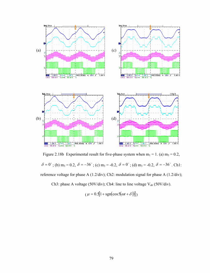
79

Figure 2.18b Experimental result for five-phase system when m1 = 1. (a) m3 = 0.2,

o0=δ ; (b) m3 = 0.2, o36−=δ ; (c) m3 = -0.2, o0=δ ; (d) m3 = -0.2, o36−=δ . Ch1:

reference voltage for phase A (1.2/div); Ch2: modulation signal for phase A (1.2/div);

Ch3: phase A voltage (50V/div); Ch4: line to line voltage Vab (50V/div).

( ( )( )[ ]δωµ ++= t5cossgn15.0 )

(a)

(b)

(c)

(d)

80

0

0.2

0.4

0.6

0.8

1

1.2

0

0.2

0.4

0.6

0.8

1

1.2

Fundamental 3rd harmonic Fundamental 3rd harmonic


the highest fundamental voltage) in the linear modulation region. (a) m1 = 0.8, m3 = -0.2;

(b) m1 = 0.8, m3 = 0.2. 1: 0=noV ; 2: 5.0=µ ; 3: ( )( )[ ]δωµ ++= t5cossgn15.0 , o0=δ ;

4: ( )( )[ ]δωµ ++= t5cossgn15.0 , o36−=δ .

0

0.2

0.4

0.6

0.8

1

1.2

0

0.2

0.4

0.6

0.8

1

1.2

Fundamental 3rd harmonic Fundamental 3rd harmonic


the highest fundamental voltage) in the over-modulation region. (a) m1 = 1.5, m3 = -0.2;

(b) m1 = 1.5, m3 = 0.2. 1: 0=noV ; 2: 5.0=µ ; 3: ( )( )[ ]δωµ ++= t5cossgn15.0 , o0=δ ;

4: ( )( )[ ]δωµ ++= t5cossgn15.0 , o36−=δ .

1 2 3 4 1 2 3 4

1 2 3 4 1 2 3 4

(a) (b)

(a) (b)

81

The phase angle between the fundamental and third harmonic voltages significantly

affects the voltage gain of the converter as illustrated in Figures 2.17 and 2.18. In many

applications, the reference voltages (equivalently, the modulation signals) and the phase

angles between them, which are the outputs of controllers, are independently determined

by closed-loop control laws. The neutral voltage signal can therefore be used to modify

the composite modulation signals in order to better the converter utility. For better results

in terms of waveform quality, voltage gain and switching loss reduction, the definitions

of µ and the selection of δ are very crucial.

2.5.6 Modulation Signals Calculation Using Turn-on Times for the Top Devices

In the carrier-based PWM, the modulation signals are calculated by adding the zero

sequence voltage to the reference signals. The final modulation signals normalized with

respect to Vd/2 are between –1 and 1 in the linear modulation region. The PWM signals

are determined by comparing the modulation signals with the triangle carrier signal with

magnitude –1 and 1.

Figure 2.21 shows the switching signals for the top devices in sector 1 in a five-

phase system. It is seen that the normalized modulation signals for the five top devices

are equal to the ratio between the individual turn-on time for the top devices and the

switching period. Thus the alternative approach of finding the modulation signal without

calculating the zero sequence voltage is to sum up the turn-on times for the top devices

and then use them as the modulation signals, which are compared with the triangle carrier

signal between 0 and 1 to generate the PWM signals. The normalized turn-on times for

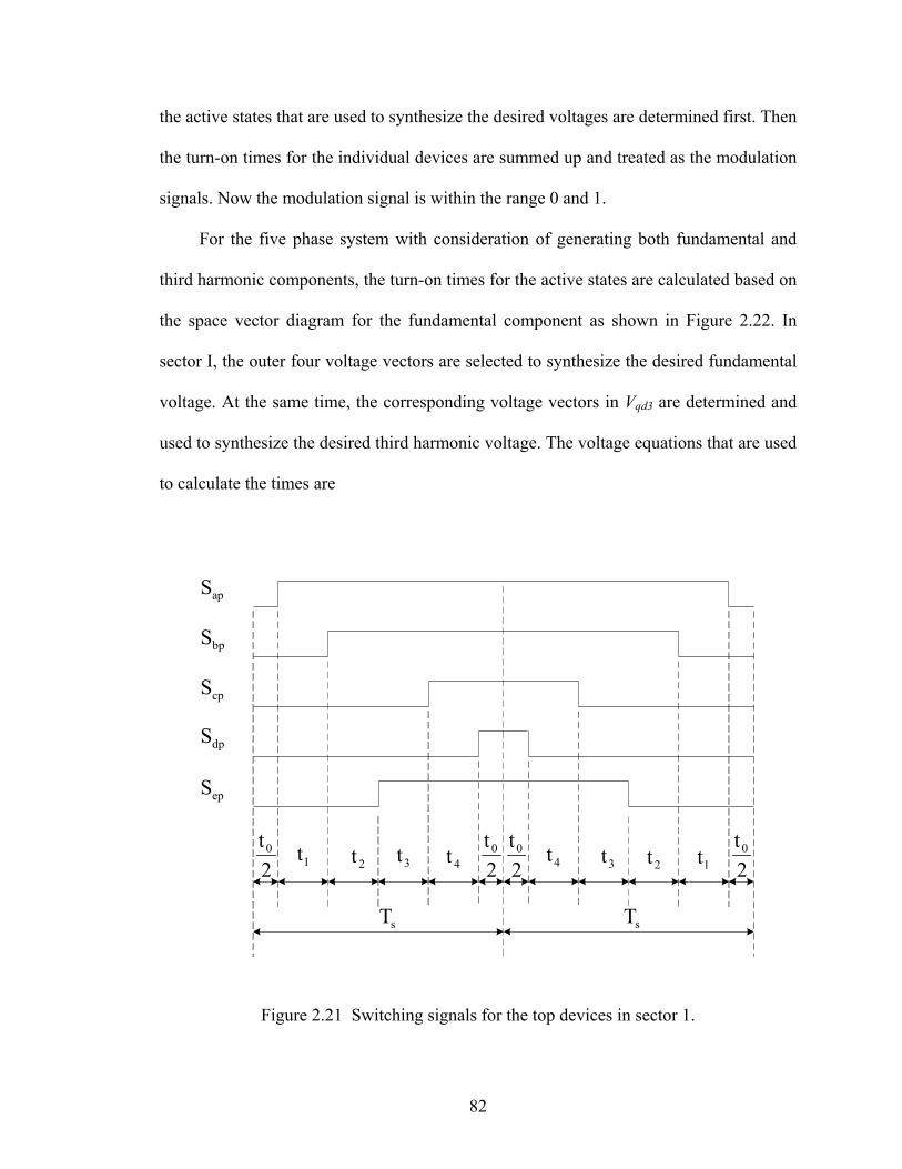
82

the active states that are used to synthesize the desired voltages are determined first. Then

the turn-on times for the individual devices are summed up and treated as the modulation

signals. Now the modulation signal is within the range 0 and 1.

For the five phase system with consideration of generating both fundamental and

third harmonic components, the turn-on times for the active states are calculated based on

the space vector diagram for the fundamental component as shown in Figure 2.22. In

sector I, the outer four voltage vectors are selected to synthesize the desired fundamental

voltage. At the same time, the corresponding voltage vectors in Vqd3 are determined and

used to synthesize the desired third harmonic voltage. The voltage equations that are used

to calculate the times are

apS

bpS

cpS

2t0

1t

dpS

epS

2t0

2t0

2t0

2t 3t 4t 4t 3t 2t 1t

sT sT

Figure 2.21 Switching signals for the top devices in sector 1.

83

032332013014343332321313

032132011014143132121111

tVtVtVtVtVtVV

tVtVtVtVtVtVV

qdqdqdqdqdqdqd

qdqdqdqdqdqdqd

+++++=

+++++=

where 4321 ,,, tttt are the corresponding times spent on the four active states as shown in

Figure 2.22. The same pattern applies to all the other sectors.

q-axis

d-axis29

204

8

7

15

13

16 17

30

26

25

24

28

182

5

931

226

1023

11 27

2114

3 1912

1 32

*1qdV

1Vv

2Vv

3Vv

4Vv

q-axis

d-axis

29

204

8

7

15

13

16 17

30

26

25

24

28

182

5

9 31

22

6

10 23

11

27

2114

3 1912

1 32

Figure 2.22 Synthesis of fundamental and third harmonic voltages in a five-phase

system. (a) Synthesizing reference voltage in sector 1 of 1qdV ; (b) Corresponding voltage

vectors in 3qdV .

(a)

(b)

84

The turn-on times for the top devices, which are the modulation signals also, are

determined as

( ) ( )[ ]( ) ( )[ ]( ) ( )[ ]( ) ( )[ ]( ) ( )[ ]43211

43211

43211

43211

43211

11

11

11

11

11

ttttmm

ttttmm

ttttmm

ttttmm

ttttmm

ee

dd

cc

bb

aa

+++−−+=

+++−−+=

+++−−+=

+++−−+=

+++−−+=

α

α

α

α

α

where 1am , 1bm , 1cm , 1dm and 1em are determined corresponding to Table 2.9.

The turn-on times for the top devices, which are the modulation signals also, are

determined as shown in Table 2.10.

Table 2.9 Calculation of the modulation signals in terms of turn-on times

Sector 1am 1bm 1cm 1dm 1em

1 4321 tttt +++ 432 ttt ++ 3t 0 32 tt +

2 421 ttt ++ 4321 tttt +++ 41 tt + 0 1t

3 32 tt + 4321 tttt +++ 432 ttt ++ 3t 0

4 1t 421 ttt ++ 4321 tttt +++ 41 tt + 0

5 0 32 tt + 4321 tttt +++ 432 ttt ++ 3t

6 0 1t 421 ttt ++ 4321 tttt +++ 41 tt +

7 3t 0 32 tt + 4321 tttt +++ 432 ttt ++

8 41 tt + 0 1t 421 ttt ++ 4321 tttt +++

9 432 ttt ++ 3t 0 32 tt + 4321 tttt +++

10 4321 tttt +++ 41 tt + 0 1t 421 ttt ++

85

Table 2.10a Calculation of the modulation signals in terms of line to line voltages

Sector 1am 1bm 1cm 1dm 1em

1 1adV + 3adV 1bdV + 3bdV 1cdV + 3cdV 0 1edV + 3edV

2 1adV + 3adV 1bdV + 3bdV 1cdV + 3cdV 0 1edV + 3edV

3 1aeV + 3aeV 1beV + 3beV 1ceV + 3ceV 1deV + 3deV 0

4 1aeV + 3aeV 1beV + 3beV 1ceV + 3ceV 1deV + 3deV 0

5 0 1baV + 3baV 1caV + 3caV 1daV + 3daV 1eaV + 3eaV

6 0 1baV + 3baV 1caV + 3caV 1daV + 3daV 1eaV + 3eaV

7 1abV + 3abV 0 1cbV + 3cbV 1dbV + 3dbV 1ebV + 3ebV

8 1abV + 3abV 0 1cbV + 3cbV 1dbV + 3dbV 1ebV + 3ebV

9 1acV + 3acV 1bcV + 3bcV 0 1dcV + 3dcV 1ecV + 3ecV

10 1acV + 3acV 1bcV + 3bcV 0 1dcV + 3dcV 1ecV + 3ecV

Table 2.10b Calculation of the modulation signals in terms of line to line voltages

Sector ( )α−1 [1-( 4321 tttt +++ )]

1 ( )α−1 [1-( 1adV + 3adV )]

2 ( )α−1 [1-( 1bdV + 3bdV )]

3 ( )α−1 [1-( 1beV + 3beV )]

4 ( )α−1 [1-( 1ceV + 3ceV )]

5 ( )α−1 [1-( 1caV + 3caV )]

6 ( )α−1 [1-( 1daV + 3daV )]

7 ( )α−1 [1-( 1dbV + 3dbV )]

8 ( )α−1 [1-( 1ebV + 3ebV )]

9 ( )α−1 [1-( 1ecV + 3ecV )]

10 ( )α−1 [1-( 1acV + 3acV )]

86

Table 2.11 Calculation of the modulation signals am in terms of line to line voltages

Sector am

1 ( 1adV + 3adV )+ ( )α−1 [1-( 1adV + 3adV )]

2 ( 1adV + 3adV )+ ( )α−1 [1-( 1bdV + 3bdV )]

3 ( 1aeV + 3aeV )+ ( )α−1 [1-( 1beV + 3beV )]

4 ( 1aeV + 3aeV )+ ( )α−1 [1-( 1ceV + 3ceV )]

5 0+ ( )α−1 [1-( 1caV + 3caV )]

6 0+ ( )α−1 [1-( 1daV + 3daV )]

7 ( 1abV + 3abV )+ ( )α−1 [1-( 1dbV + 3dbV )]

8 ( 1abV + 3abV )+ ( )α−1 [1-( 1ebV + 3ebV )]

9 ( 1acV + 3acV )+ ( )α−1 [1-( 1ecV + 3ecV )]

10 ( 1acV + 3acV )+ ( )α−1 [1-( 1acV + 3acV )]

The proposed method of using the turn-on times for the top switching devices as the

modulation signals is implemented to generate both fundamental and third harmonic

voltages. The carrier-based PWM is used to generate the PWM signals through

comparing the modulation signals with the high-frequency triangle signal with magnitude

between 0 and 1. Figures 2.23 and 2.24 show the experimental results when the inverter

is operating in the linear modulation region. The third harmonic voltage with

magnitude 2.03 =m is subtracted from and added to the fundamental voltage with

magnitude 7.01 =m in Figures 2.23 and 2.24 respectively. Figures 2.25 and 2.26 shows

the experimental results when the inverter is operating in the over-modulation region, in

which 4.11 =m and 2.03 =m . The third harmonic voltage is subtracted from and added

to the fundamental voltage in Figure 2.25 and Figure 2.26, respectively.

87

Different modulation schemes are implemented to see the effects. The first one is

the space vector modulation when 5.0=µ while the second and third ones are

corresponding to the discontinuous modulations when oo 36,0 −=δ . It is seen that the

modulation signals at the middle are flattened when the peaks of the two reference

voltages are out of phase with each other. When the neutral voltage corresponding to

5.0=µ is added to the reference voltage signals, the flatness of the middle portion of the

composite modulation signal increases, which means that a higher fundamental voltage

can be generated in the linear region compared to the condition when the neutral voltage

is excluded from the modulation signal expression. However, this kind of flatness cannot

be observed when the third harmonic voltage is in phase with the fundamental voltage.

In the case of discontinuous PWM with different angle δ , the waveforms can be

appropriately shifted with respect to the fundamental voltage to clamp at the appropriate

regions of the phase current waveforms and to change the converter voltage gain.

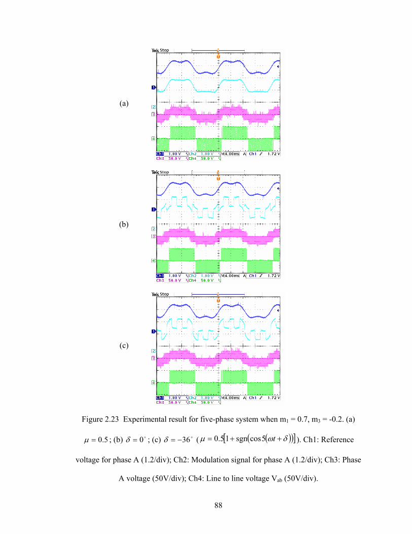
88



voltage for phase A (1.2/div); Ch2: Modulation signal for phase A (1.2/div); Ch3: Phase

A voltage (50V/div); Ch4: Line to line voltage Vab (50V/div).

(a)

(b)

(c)

89



voltage for phase A (1.2/div); Ch2: Modulation signal for phase A (1.2/div); Ch3: Phase

A voltage (50V/div); Ch4: Line to line voltage Vab (50V/div).

(a)

(b)

(c)

90





(a)

(b)

(c)

91





(a)

(b)

(c)

92

2.6 Conclusion

This chapter shows the equivalence between the carrier-based PWM and space

vector PWM for the three-phase system through derivation of the modulation scheme.

Then the modulation technique is extended to the multi-phase system in the example of

five and six phases. The generalized transformation is defined and the concept of space

vector is applied to calculate the zero sequence voltage expressions in all sectors by

choosing the appropriate active and null states. Then these expressions are generalized

and added to the reference voltage to generate the modulation signals. The experimental

results for the five-phase system validate the possibility of generating the voltages more

than the fundamental one and this approach can be used to drive two machines in series.

93

CHAPTER 3

INDUCTION MACHINE MODEL

3.1 Introduction

Induction motors have been widely used in the industrial drive system as a means of

converting electric power to mechanical power. With the development of the vector

control technology, the induction machine drive systems offer high performance as well

as independent control on torque and flux linkages, which is similar to that of the DC

machine. Furthermore, it is possible to drive the induction machines above their rated

speed through flux weakening, which also finds a lot of industrial applications.

In this chapter, the operation principle of a three-phase induction motor is

explained. Then the stator and rotor voltage equations and the torque equations are

derived. The transformation to the arbitrary reference frame is established for the

convenience of analysis. These equations are the basis that is necessary for the analysis of

vector control and any other control approach.

3.2 Operation Principle of a Three-phase Induction Motor

Any type of induction motors can be represented by a simplified model with two

poles. The winding arrangement of a two-pole, three-phase, wye-connected symmetrical

induction motor is shown in Figure 3.1. The stator windings are identical with equivalent

turns and resistance. The rotor windings are also approximated as identical windings with

94

equivalent turns and resistance, which may be a forged squirrel cage type or a wound

type. Both stator and rotor windings are approximated as sinusoidally distributed

windings and the air gap is assumed uniform.

In general, the induction motor is operated with the stator windings connected to a

balanced three-phase voltage source and the rotor windings short-circuited. The balanced

three-phase current is then generated in the stator windings, which are sinusoidally

distributed in space with 120° electrical degrees phase shift. These currents with the help

of stator winding distribution establish a rotating air-gap magneto-magnetic force (MMF)

rω

as axis

cr axis

cs axis

bs axis

br axis

cs'

ar

cr'

as

cr

br

bs

as'

ar'cs

br'

bs'

rθ

ar axisrφ

sφ

Figure 3.1 Two-pole, three-phase, wye-connected symmetrical induction motor.

95

as in the case of the synchronous machine, which rotates about the air gap at the speed

determined by the stator voltages/currents frequency and the number of poles.

( ) me P ωω 2/= (3.1)

where me ωω and are the electrical and mechanical speeds in radian/second and P is the

number of poles of stator windings. When the rotor speed in electrical degrees is different

from this synchronous speed, three-phase balanced currents will be induced in the rotor

windings to counter the change of flux linkages from Lenz's law. The difference between

the rotor speed in electrical degrees and the synchronous speed is defines as the slip

frequency.

res ωωω −= (3.2)

This is the frequency of the current flowing in the rotor windings. The induced rotor

currents also produce an air-gap MMF, which rotates at the speed corresponding to the

frequency of rotor currents relative to the rotor. It means that the air-gap MMF generated

from the stator currents rotates at the same speed of that established from the rotor

currents. These two MMFs can be seen as two sets of magnetic poles and they are

interacted with each other to produce the torque. It is clear that two MMFs have to exist

in order to generate the electric torque, which can be resulted from the currents or excited

from the permanent magnets as in the permanent magnet machine. In the case of

induction motor, they are generated from both currents in the stator and rotor windings,

which mean the rotor speed in electrical degrees has to be different from the synchronous

speed in order to produce the electric torque and run the motor. Otherwise there is no

current induced in the rotor windings and therefore no toque produced. The induction

machine is classified into motoring and generating modes depending on the sign of the

96

slip frequency. If the slip frequency is greater than zero, the machine is running as an

induction motor and the electric power is consumed by the machine and converted into

mechanical power through the rotor. The stator current flows into the machine. If the slip

frequency is less than zero, the machine runs as an induction generator and the stator

current flows out of the stator. The mechanical power from the rotor shaft is then

transformed into electric power and then consumed by the load connected to the stator.

3.3 Three-phase Induction Motor Voltage Equations

A two-pole, three-phase wye-connected induction machine is shown in Figure 3.1.

The stator windings of which are identical, sinusoidally distributed in space with a phase

displacement of 120° (electrical degrees), with Ns equivalent turns and phase resistance,

rs. Similarly, the rotor is assumed to be symmetrical with three-phase windings displaced

in space by the angle of 120° (electrical degrees), with Nr equivalent turns and phase

resistance rr. The voltage equations for the stator and the rotor are given as

cscsscs

bsbssbs

asassas

pIrV

pIrV

pIrV

λ

λ

λ

+=

+=

+=

(3.3)

crcrrcr

brbrrbr

ararrar

pIrV

pIrV

pIrV

λ

λ

λ

+=

+=

+=

(3.4)

where Vas, Vbs, and Vcs are the three-phase stator voltages with the supply frequency while

Var, Vbr, and Vcr are the three-phase rotor voltages induced from the stator with the slip

frequency. Ias, Ibs, and Ics are the three-phase stator currents while Iar, Ibr, and Icr are the

97

three-phase rotor currents. rs and rr are the stator and rotor phase resistance respectively.

λas, λbs, and λcs are the three-phase stator flux linkages while λar, λbr, and λcr are the three-

phase rotor flux linkages. p represents the derivative term d/dt. The above relationship

can be seen clearly after the space model of the induction motor is expressed as the phase

circuit model as shown in Figure 3.2.

Then it is necessary to derive the machine inductances in order to have the

equivalent circuit model. In a magnetically linear system, the self-inductance of a

winding is the ratio of the flux linked by a winding to the current flowing in the same

winding with all other winding currents zero. Mutual inductance is the ratio of flux linked

by one winding due to the current flowing in a second winding with all other winding

currents zero. In the case of the induction machine, the air-gap is uniform. So the flux

density due to current in the as winding with all other currents zero is obtained as

sr

asV

asI

sN

bsI

csI

bsV

sNsN

sr srcsV

rr

arV

arI

rN

brI

crI

brV

rNrN

rr rrcrV

Figure 3.2 The equivalent phase circuit model of the induction machine.

98

( ) ( )

( )sass

ssa

IN

gB

φµ

φµφ

cos2

MMF

0

0

=

⋅=

(3.5)

where g is the length of the air-gap and sφ is the angular displacement of the stator.

Similarly, the flux density with all currents zero except Ibs and Ics are

( )

( ) ⎟⎠⎞

⎜⎝⎛ +=

⎟⎠⎞

⎜⎝⎛ −=

32cos

2

32cos

2

0

0

πφµφ

πφµφ

scss

sc

sbss

sb

IN

B

IN

B

(3.6)

Then the flux is determined by performing a surface integral over the open surface

of a single turn as

( ) ( )∫+

=Φπφ

φξξφ s

s

rldBas (3.7)

where r is the average radius of the air gap of the machine and l is the axial length of the

air gap. For the sinusoidally distributed as winding, the turns function can be expressed

as

( ) ( )ss

sasN

N φφ sin2

−= (3.8)

So the total flux linkages of the as winding due to the current flowing only in the as

winding is

( ) ( )

ass

asls

sasasaslsas

Ig

rlNIL

drldBNIL s

s

πµ

φξξφλπφ

φ

02

2 ⎟

⎠⎞

⎜⎝⎛+=

+= ∫ ∫+

(3.9)

The self-inductance of the as winding is obtained by dividing the above equation by

Ias.

99

msls

slsasas

LL

grlN

LL

+=

⎟⎠⎞

⎜⎝⎛+=

πµ02

2 (3.10)

where msL is the stator magnetizing inductance. The self-inductances of phase b and c

have the same expression since the three phases are assumed symmetrical.

The mutual inductance between the two stator windings as and bs can be

determined in the similar way by first computing the flux linking the as winding due to

the current flowing in the bs winding. In this case,

( ) ( )

bss

sbsasas

Ig

rlN

drldBN s

s

πµ

φξξφλπφ

φ

02

221 ⎟

⎠⎞

⎜⎝⎛−=

= ∫ ∫+

(3.11)

The mutual inductance between as winding and bs winding is obtained by dividing

the above equation by Ibs.

ms

sasbs

L

grlN

L

21

221 0

2

−=

⎟⎠⎞

⎜⎝⎛−=

πµ

(3.12)

The mutual inductances between phase b and c and between phase c and a have the

same expression since the three phases are assumed symmetrical.

It follows that the rotor self-inductances for three phases are equal to

mrlr

rlsarar

LL

grlNLL

+=

⎟⎠⎞

⎜⎝⎛+=

πµ02

2 (3.13)

where mrL is the rotor magnetizing inductance.

100

The mutual inductances between any two rotor windings are

mr

rarbr

L

grlNL

21

221 0

2

−=

⎟⎠⎞

⎜⎝⎛−=

πµ

(3.14)

The mutual inductances between the stator and rotor windings can be determined

using the same method. All of these mutual inductances are

grlNN

L rssr

πµ0

22⎟⎠⎞

⎜⎝⎛⎟⎠⎞

⎜⎝⎛= (3.15)

rsrrbsbrasar LLLL θcoscsc === (3.16)

⎟⎠⎞

⎜⎝⎛ +===

32cos πθ rsrcsarbscrasbr LLLL (3.17)

⎟⎠⎞

⎜⎝⎛ −===

32cos πθ rsrcsbrbsarascr LLLL (3.18)

Then the flux linkages for the stator windings can be written as

crrbrcsbrarcsarcssbscsbsascsascs

crbscrbrbsbrarbsarcsbscsbsbsbsasbsasbs

crascrbrasbrarasarcsascsbsasbsasasasas

ILILILILILIL

ILILILILILIL

ILILILILILIL

csccsc +++++=

+++++=

+++++=

λ

λ

λ

(3.19)

And the flux linkages for the rotor windings are

crcrcrbrcrbrarcrarcscrcsbscrbsascrascr

crbrcrbrbrbrarbrarcsbrcsbsbrbsasbrasbr

crarcrbrarbrarararcsarcsbsbrbsasarasar

ILILILILILIL

ILILILILILIL

ILILILILILIL

+++++=

+++++=

+++++=

λ

λ

λ

(3.20)

101

3.4 Reference Frame Transformation

In the above derivations, all signals including phase voltages and currents are time-

changing and all the inductances are time-changing also. All these ac variables increase

the complexity of analyzing the machine. Fortunately various transformation theories

were established to make the analysis in a much easier way. The basic idea is to

transform the ac signals into dc signals, which are constant corresponding to a particular

operating condition. After the analysis is done and the result comes out, the results are

then transformed back to get the ac signals through the inverse transformation. This

process is realized by the transformation between the stationary and synchronous

reference frames, which are rotating at zero and synchronous ( eω ) speeds. However, this

reference frame can be rotating at any arbitrary speed in general. So it is desired to get the

general form of the transformation and then apply it in the particular applications.

(q-axis)

(d-axis)bf

( )sqa ff

cf

θ

ω

sdf

df

qf

Figure 3.3 Transformation between reference frames.

102

The general transformation from the stationary abc reference frame to qd0 reference

frame rotating at the arbitrary speed ω (rad/s) is shown in Figure 3.3 and defined in

(3.21).

⎥⎥⎥

⎦

⎤

⎢⎢⎢

⎣

⎡⋅=

⎥⎥⎥

⎦

⎤

⎢⎢⎢

⎣

⎡

⎥⎥⎥⎥⎥⎥⎥

⎦

⎤

⎢⎢⎢⎢⎢⎢⎢

⎣

⎡

⎟⎠⎞

⎜⎝⎛ +⎟

⎠⎞

⎜⎝⎛ −

⎟⎠⎞

⎜⎝⎛ +⎟

⎠⎞

⎜⎝⎛ −

=⎥⎥⎥

⎦

⎤

⎢⎢⎢

⎣

⎡

c

b

a

c

b

a

d

q

fff

Kfff

fff

21

21

21

32sin

32sinsin

32cos

32coscos

32

0

πθπθθ

πθπθθ

(3.21)

where 0θωθ += t , which represents the instant angle between two reference frames. f

can be any variable in the corresponding reference frame including voltages, currents,

flux linkages, inductance, etc.

In the case of transforming the variables in the abc stationary reference frame into

the synchronous reference frame, eωω = . The transformation can be done using (3.21)

directly. However, six sine/cosine functions are necessarily calculated, which introduce a

lot of calculation burden and not preferred especially in the digital implementation. The

alternative way is to transform states in the abc stationary reference frame into the qd0

stationary reference frame (Clarke transformation). And then the final transformation is

done through transforming the states in the qd0 stationary reference frame in to the qd0

synchronous reference frame (Park transformation). By this way, only two sine/cosine

functions are calculated, which save a lot of calculation time. The Clarke transformation

can be derived from the general transformation expression by forcing 0=ω .

103

( )

( )cbas

cbs

d

cbas

q

ffff

fff

ffff

++=

+−=

⎟⎠⎞

⎜⎝⎛ −−=

31

31

21

21

32

0

(3.22)

Note that the third expression, which represents the zero sequence component,

remains the same in the arbitrary reference frame. So it will not be put together with the

qd expressions in the following analysis. Assuming the states in the abc stationary

reference frame are balanced, which means

0=++ cba fff (3.23)

Then the Clarke transformation is rewritten as

( )

( )

( )ca

ba

cbs

d

as

q

ff

ff

fff

ff

23

1

23

1

31

+=

−−=

+−=

=

(3.24)

From Figure 3.3, the Park transformation between the qd0 stationary and

synchronous reference frames is

⎥⎦

⎤⎢⎣

⎡⎥⎦

⎤⎢⎣

⎡ −=⎥

⎦

⎤⎢⎣

⎡s

d

sq

d

q

ff

ff

θθθθ

cossinsincos

(3.25)

After the analysis is done in the synchronous reference frame, the results need to be

transformed back into the abc stationary reference frame. The general inverse

transformation is

104

⎥⎥⎥

⎦

⎤

⎢⎢⎢

⎣

⎡⋅=

⎥⎥⎥

⎦

⎤

⎢⎢⎢

⎣

⎡

⎥⎥⎥⎥⎥⎥⎥

⎦

⎤

⎢⎢⎢⎢⎢⎢⎢

⎣

⎡

⎟⎠⎞

⎜⎝⎛ +⎟

⎠⎞

⎜⎝⎛ +

⎟⎠⎞

⎜⎝⎛ −⎟

⎠⎞

⎜⎝⎛ −=

⎥⎥⎥

⎦

⎤

⎢⎢⎢

⎣

⎡−

0

1

01

32sin

32cos

13

2sin3

2cos

1sincos

fff

Kfff

fff

d

q

d

q

c

b

a

πθπθ

πθπθ

θθ

(3.26)

The inverse Park and Clarke transformations are

⎥⎦

⎤⎢⎣

⎡⎥⎦

⎤⎢⎣

⎡−

=⎥⎦

⎤⎢⎣

⎡

d

qs

d

sq

ff

ff

θθθθ

cossinsincos

(3.27)

sd

sqc

sd

sqb

sqa

fff

fff

ff

23

21

23

21

+−=

−−=

=

(3.28)

3.5 Three-phase Induction Motor Equivalent Circuit

To facilitate the following analysis, the abbreviations are used

[ ]

[ ]Tcrbrarabcr

Tcsbsasabcs

ffff

ffff

=

= (3.29)

Then the flux linkages in the stator and rotor windings can be expressed in terms of

the stator and rotor currents as

⎥⎦

⎤⎢⎣

⎡⎥⎦

⎤⎢⎣

⎡=⎥

⎦

⎤⎢⎣

⎡

abcr

abcs

rT

sr

srs

abcr

abcs

II

LLLL

λλ

(3.30)

and

105

⎥⎥⎥⎥⎥⎥

⎦

⎤

⎢⎢⎢⎢⎢⎢

⎣

⎡

+−−

−+−

−−+

=

mslsmsms

msmslsms

msmsmsls

s

LLLL

LLLL

LLLL

L

21

21

21

21

21

21

(3.31)

⎥⎥⎥⎥⎥⎥

⎦

⎤

⎢⎢⎢⎢⎢⎢

⎣

⎡

+−−

−+−

−−+

=

mrlsmrmr

mrmrlrmr

mrmrmrlr

r

LLLL

LLLL

LLLL

L

21

21

21

21

21

21

(3.32)

( ) ( ) ( )( ) ( ) ( )( ) ( ) ( ) ⎥

⎥⎥

⎦

⎤

⎢⎢⎢

⎣

⎡

−++−−+

=

rrr

rrr

rrr

srsr LLθβθβθ

βθθβθβθβθθ

coscoscoscoscoscoscoscoscos

(3.33)

where 3

2πβ = .

In order to derive the equivalent circuit, it is necessary to transform all signals into

the same side of the machine, either stator side or rotor side. And there is a turn ratio

between these two sides corresponding to the definition of flux linkages. It is preferred to

transform the flux linkages on the rotor side into the stator side. Then the flux linkages

and the voltage equations are expressed in terms of machine variables referred to the

stator windings as

( )( ) ⎥

⎦

⎤⎢⎣

⎡

⎥⎥⎦

⎤

⎢⎢⎣

⎡=⎥

⎦

⎤⎢⎣

⎡'''

'

'abcr

abcs

rT

sr

srs

abcr

abcs

II

LLLL

λλ

(3.34)

( ) ⎥⎦

⎤⎢⎣

⎡

⎥⎥⎦

⎤

⎢⎢⎣

⎡

+

+=⎥

⎦

⎤⎢⎣

⎡''''

'

'abcr

abcs

rrT

sr

srss

abcr

abcs

II

pLrLppLpLr

VV

(3.35)

where

106

abcrs

rabcrabcr

s

rabcrabcr

s

rabcr N

NVNNVI

NNI λλ === ''' , ,

rr

srr

s

rrsr

s

rsr L

NN

LrNN

rLNN

L2

'2

'' , , ⎟⎟⎠

⎞⎜⎜⎝

⎛=⎟⎟

⎠

⎞⎜⎜⎝

⎛== .

In order to facilitate the analysis, the voltage equations are generally transformed

into the synchronous reference frame. This process is done through multiplying both

sides of (3.34 ~ 35) by K.

( )( ) ( ) ⎥

⎦

⎤⎢⎣

⎡⋅⋅⋅

⎥⎥⎦

⎤

⎢⎢⎣

⎡⋅=⎥

⎦

⎤⎢⎣

⎡⋅ −

'1

''

'

'abcr

abcs

rT

sr

srs

abcr

abcs

II

KKLLLL

KKλλ

( ) ( ) ⎥⎦

⎤⎢⎣

⎡⋅⋅⋅

⎥⎥⎦

⎤

⎢⎢⎣

⎡

+

+⋅=⎥

⎦

⎤⎢⎣

⎡⋅ −

'1

'''

'

'abcr

abcs

rrT

sr

srss

abcr

abcs

II

KKpLrLp

pLpLrK

VV

K

After substituting the transformation matrix intro this expression,

( )( ) ⎥

⎦

⎤⎢⎣

⎡⋅

⎥⎥⎦

⎤

⎢⎢⎣

⎡

⋅⋅⋅⋅

⋅⋅⋅⋅⋅=⎥

⎦

⎤⎢⎣

⎡−−

−−

'0

0

1'1'

1'1

'0

0

rqd

sqd

rT

sr

srs

rqd

sqd

II

KLKKLKKLKKLK

λλ

( ) '0

''0

''0

000

rqddqrrrqdrrqd

sqddqssqdssqd

pIrV

pIrV

λλωω

λωλ

+−+=

++= (3.36)

where

[ ]Tsdsqssqd 00 λλλλ = , [ ]Trdrqrrqd'

0'''

0 λλλλ = ,

[ ]Tqsdsdqs 0λλλ = , [ ]Tqrdrdqr 0''' λλλ = ,

⎥⎥⎥

⎦

⎤

⎢⎢⎢

⎣

⎡+

+=⋅⋅ −

ls

mls

mls

s

LLL

LLKLK

000000

1 ,

107

⎥⎥⎥

⎦

⎤

⎢⎢⎢

⎣

⎡

++

=⋅⋅ −

'

'

'

1'

000000

lr

mlr

mlr

r

LLL

LLKLK ,

( ) ( )⎥⎥⎥

⎦

⎤

⎢⎢⎢

⎣

⎡=⋅⋅=⋅⋅ −−

0000000

1'1'm

mT

srsr LL

KLKKLK ,

msm LL23

= .

These voltage equations are frequently written in expanded form.

ssss

dsqsdssds

qsdsqssqs

pIrV

pIrV

pIrV

000 λ

λωλ

λωλ

+=

+−=

++=

(3.37)

( )

( )'

0'

0''

0

'''''

'''''

rrrr

drqrrdrrdr

qrdrrqrrqr

pIrV

pIrV

pIrV

λ

λλωω

λλωω

+=

+−−=

+−+=

(3.38)

And the expressions for the flux linkages in expanded form are

( )( )

slss

drdsmdslsds

qrqsmqslsqs

IL

IILIL

IILIL

00

'

'

=

++=

++=

λ

λ

λ

(3.39)

( )( )

'0

''0

''''

''''

rlrr

drdsmdrlrdr

qrqsmqrlrqr

IL

IILIL

IILIL

=

++=

++=

λ

λ

λ

(3.40)

From (3.37 ~ 40), the qd0 equivalent circuit of the induction machine in an arbitrary

reference frame rotating at speed ω is shown in Figure 3.4. The equivalent circuit in the

108

synchronous reference frame can be derived by making eωω = . The advantage of using

the synchronous reference frame is that the applied voltages after the transformation are

DC quantities and then the currents can be solved easily. Since all the quantities in the

rotor are referred to the stator side in the convenience of analysis, the sign of “prime” in

the rotor equations will be ignored in the following analysis.

The dynamic equation of the induction machine is given as

( )Ler TTJ

Pp −=2

ω (3.41)

in which the electric torque can be calculated using flux linkages and currents as

qsωλlsLsr

dsV dsImL

'lrL

dsωλlsLsr

qsVqsI

mL

'lrL

( ) 'qrr λωω −

'rr

'drI

( ) 'drr λωω − '

rr

'qrI

'drV

'qrV

lsLsr

sV0sI0

'lrL '

rr

'0rI

'0rV

Figure 3.4 The qd0 equivalent circuit model of the induction machine in the arbitrary

reference frame.

109

( )

( )

( )dsqsqsds

dsqrqsdrm

dsqrqsdrr

me

IIP

IIIILP

IILLPT

λλ

λλ

−⋅=

−⋅⋅=

−⋅⋅=

43

43

43

(3.42)

3.5.1 Induction Machine Model Using Natural Variables

The variables of the natural variable model of the induction machine are chosen as

the developed electromagnetic torque eT , the developed reactive torque rT , the rotor

speed rω , and the square of the magnitude of the rotor flux linkage rrλ . These variables

are the same in all reference frames or independent of the selected reference frame. These

natural variables are expressed in terms of the axis currents and flux linkages as:

( )( )

22drqrrr

qsqrdsdrtr

dsqrqsdrte

IIkT

IIkT

λλλ

λλ

λλ

+=

+=

−=

(3.49)

where r

mt L

PLk4

3= and P is the poles of the machine.

The stator and rotor voltage equations can be rewritten in terms of stator currents

and rotor flux linkages as

( )( ) qrrdrdrr

drrqrqrr

dsqrr

mrdrdsds

qsdrr

mrqrqsqs

pIr

pIr

pILLL

crIV

pILLL

crIV

λωωλ

λωωλ

λω

λ

λω

λ

σ

σ

−−+=

−++=

+−−=

++−=

0

0

(3.50)

110

where 2

2

r

mrs

LLr

kr

r += , 2r

mr

LLr

c = .

To obtain the desired model, equations (3.49) are differentiated and then expressed

in terms of the defined natural variables as follows.

1mkL

kLLLk

TTLLLr

kLr

pT trrr

r

mtrre

r

srse

σσσσ

λωω +−−⎟⎟⎠

⎞⎜⎜⎝

⎛+−= (3.51)

( )Ler TTJ

Pp −=2

ω (3.52)

22

22

mkL

kLLLrk

TTT

kLLr

TLLLr

kLr

pT

trr

r

mrt

errr

re

tr

mrr

r

srsr

σσ

σσ

λ

ωλ

++

++

+⎟⎟⎠

⎞⎜⎜⎝

⎛+−=

(3.53)

rrt

mrrr

r

rrr T

LkLr

Lrp

22+−= λλ (3.54)

where

dsdrqsqr

dsqrqsdr

VVm

VVm

λλ

λλ

+=

−=

2

1 (3.55)

The quantities 1m and 2m are calculated using the outputs of the controllers for eT

and rT . Then the voltages commands are calculated by solving (3.55).

rr

qrdrds

rr

qrdrqs

mmV

mmV

λλλ

λλλ

12

21

−=

+=

(3.56)

The natural variables model of the induction machine can also be expressed in

terms of the stator flux in place of the rotor flux. The model equations are derived as

111

below. The method used in the derivation is the same as that used for the model of the

natural variables in terms of the rotor flux. The natural variables are defined as follows.

( )( )

22dsqsss

dsdsqsqsr

dsqsqsdse

IIkT

IIkT

λλλ

λλ

λλ

+=

+−=

−=

(3.57)

where 4

3Pkt = .

To obtain the desired model, equations (3.57) are differentiated and then expressed

in terms of the defined natural variables as follows.

⎥⎦

⎤⎢⎣

⎡−−⎟⎟

⎠

⎞⎜⎜⎝

⎛+−= ss

rrre

r

srse L

kTTLLrr

LmkpT λωω

σσ

13 (3.58)

( )224

1re

ss

serr

r

srsss

r

rr TT

krTT

LLrr

LLLrmkpT +++⎟⎟

⎠

⎞⎜⎜⎝

⎛+−⎟⎟

⎠

⎞⎜⎜⎝

⎛−=

λωλ

σσ

(3.59)

( ) rs

dsdsqsqsss TkrVVp 22 −+= λλλ (3.60)

where

dsqsqs

qsdsds V

LIL

VL

ILm ⎟⎟⎠

⎞⎜⎜⎝

⎛ −−⎟⎟

⎠

⎞⎜⎜⎝

⎛ −=

σ

σ

σ

σ λλ3

dsdsds

qsqsqs V

LILV

LIL

m ⎟⎟⎠

⎞⎜⎜⎝

⎛ +−⎟⎟

⎠

⎞⎜⎜⎝

⎛ +−=

σ

σ

σ

σ λλ4 .

Equations (3.58) to (3.60) are the model equations for the induction machine in

terms of the natural variables Te, Tr and λss.

112

3.5.2 Induction Machine Model Using Flux Linkages

The voltage equations of the induction machine can be expressed in terms of the

stator and rotor flux linkages, which find the applications in the flux observers. In the

arbitrary reference frame, the complex form is adopted for all quantities in q-d axis to

simplify the analysis as follows.

drqrqdrdsqsqds

drqrqdrdsqsqds

drqrqdrdsqsqds

jj

jIIIjIII

jVVVjVVV

λλλλλλ +=+=

+=+=

+=+=

,

,

,

The stator and rotor voltage equations of an induction machine are

qdseqdsqdssqds jpIrV λωλ −+= (3.61)

qdrreqdrqdrrqdr jpIrV λωωλ )( −−+= (3.62)

The currents in the equations are substituted with the flux linkages to generate the

state equations in terms of the flux linkages using

qdrmqdssqds ILIL +=λ

qdsmqdrrqdr ILIL +=λ

Define r

ms L

LLL

2

−=σ and express the currents in terms of the flux linkages as

qdrr

mqdsqds LL

LL

I λλσσ

−=1 (3.63)

qdrr

sqds

r

mqdr LL

LLL

LI λλ

σσ

+−= (3.64)

The stator and rotor voltage equations can be rewritten as

113

qdseqdsqdrr

msqds

sqds jp

LLLr

Lr

V λωλλλσσ

−+−= (3.65)

( ) qdrreqdrqdrr

srqds

r

mrqdr jp

LLLr

LLLr

V λωωλλλσσ

−−+−+−= (3.66)

3.6 Parameters of Induction Machines

The parameters of the induction machine are very important for the analysis and

especially for the implementation of control system. The determination of the parameters

involves three different tests, the dc test, no-load test and blocked rotor test. The phase

model shown in Figure 3.5 is used to determine the phase parameters of the machine

assuming that three phases are symmetrical. The stator core loss is represented by the

core loss resistance in parallel with the mutual inductance. And the slip is defined as

e

resωωω −

= (3.67)

The stator resistances of the testing induction motor are calculated by measuring the

phase current when a DC voltage is applied between two phases (The DC voltage is

applied to the phase to neutral when the neutral point is accessible). The average value of

the three measurements is then divided by two to calculate the phase resistance.

lsLsr

phV

phI

mL

'lrL

srr

'cr

Figure 3.5 The phase model of the induction machine.

114

dc

dcs I

Vr2

= (3.68)

The second test performed is the no-load test, which is used to calculate the

magnetizing inductance and the core loss resistance. The three-phase balanced voltage

with normal frequency is applied to the induction machine that is disconnected from the

load and then the phase currents and the total active power are measured. In this case, the

slip is nearly zero. The assumption is made for the calculations that the core loss

resistance is big compared with the impedance due to the mutual inductance and the

voltage drop on the stator resistance is small. The equations in (3.69) are used to calculate

the relationship between the mutual inductance and phase voltage and the relationship

between the core loss resistance and phase voltage.

( )

Pr

VIr

IV

LLjr

c

phphs

ph

phmlss

=+

=++

22 33

ω

(3.69)

The third test performed is the blocked rotor test, which is used to calculate the

leakage inductances and the rotor resistance. The three-phase balanced voltage is applied

to the induction machine, the rotor of which is held stationary. Then the phase currents

and the total active power are measured. In this case, the slip is nearly unity. The

impedance of the core loss resistance and the mutual inductance is big compared with the

impedance of the rotor leakage inductance and rotor resistance. So the equations in (3.70)

are applied to calculate the leakage inductances by assuming the stator leakage

inductance is equal to the rotor leakage inductance.

115

( ) ( )

( ) PIrr

IV

LLjrr

phrs

ph

phlrlsrs

=+

=+++

2'

''

3

ω (3.70)

0

25

50

75

100

0 40 80 120 160Vph (V)

Xm (O

hm)

0

250

500

750

1000

0 40 80 120 160

Vph (V)

Rm

(Ohm

)

Figure 3.6 No-load test: (a) Mutual impedance vs phase voltage, (b) equivalent core loss

resistance vs phase voltage.

(a)

(b)

116

It is shown that the equivalent core loss resistance is much greater than the

corresponding mutual impedance in the no-load test, which means that the core loss can

be ignored in the analysis. All of these parameters are changing with respect to the phase

voltages and/or currents. So the average values are used in the following analysis. The

parameters of the experimental induction motor are shown in Table 3.1.

As it can be seen from Figure 3.6, the core loss is not negligible when the induction

machine is running at low supply voltage. The stator core loss has to be considered

especially when the total electrical loss is to be minimized. The stationary reference

frame q-d equivalent circuit of the induction machine with consideration of stator core

loss is shown in Figure 3.8, in which the core loss is represented by the power consumed

by the core loss resistance.

In order to analyze the machine, the machine voltage equations are expressed in

terms of the toque effective currents instead of the actual input currents. These currents

are 'qsI and '

dsI in the stationary q-d reference frame. When the stator core loss is

neglected, these two currents are identical to qsI and dsI , respectively. The voltage

equations considering the stator core loss are given as

Table 3.1 Parameters of the experimental induction motor

9812.1=sR Ω 0091.0=lsL H

85.1=rR Ω 0091.0=lrL H

1986.0=mL H 4=P

117

0

4

8

12

16

0 10 20 30 40

Vph (V)

X1+X

2 (o

hm)

Figure 3.7 Blocked rotor test: leakage impedance vs phase voltage.

qsωλlsLsr

dsV dsI

- +'dsI

cr cdImL

lrL

dsωλlsLsr

qsVqsI

mL

+ -'qsI

cr cqI

lrL

( ) qrr λωω −

+ -rr

drI

( ) drr λωω −

- +rr

qrI

drV

qrV


resistance.

118

qrrdrdrr

drrqrqrr

dsqrr

mrdrds

ds

qsdrr

mrqrqs

qs

pIr

pIr

pILLL

crIk

V

pILLL

crIk

V

λωλ

λωλ

λω

λ

λω

λ

σ

σ

++=

−+=

+−−=

++−=

0

0

''

''

(3.45)

where 2

2

r

mrs

LLr

kr

r += , 2r

mr

LLr

c = .

3.7 Conclusion

This chapter presented the induction machine model in both stationary and the

arbitrary reference frames. The general transformations between different reference

frames are derived, which are used to get the voltage equations in the arbitrary reference

frame. The procedure of determining induction machine parameters is illustrated through

the test on the experimental machine.

119

CHAPTER 4

VECTOR CONTROL OF INDUCTION MACHINE

4.1 Introduction

Induction motors have been widely used in the industrial drive system as a means of

converting electric power to mechanical power. With the development of the vector

control technology, the induction machine drive systems offer high performance as well

as independent control on torque and flux linkages, which is similar to that of the DC

machine. Furthermore, it’s possible to drive the induction machines above their rated

speed through flux weakening, which also finds a lot of industrial applications. The major

applications include pumps, fans, electric vehicles, machine tools, robotics, and many

kinds of electric propulsions. The vector control is referred for controlling both amplitude

and phase of the AC excitation. And the vector control of voltages and currents results in

the control of spatial orientation of the electromagnetic fields in the machine, which leads

to the field orientation. It is usually desired to have the 90° orientation between the MMF

due to the armature current and the field.

The control schemes available for the induction motor drives are the scalar control,

direct torque control, adaptive control, and vector or field oriented control. The vector

control is mainly discussed in this chapter. In the case of induction machines, the rotor

flux oriented control is usually employed although it is possible to implement stator flux

oriented and also magnetizing flux oriented control. The stator/rotor flux linkages of the

induction machines are necessary for the vector control. In terms of the methods of

120

obtaining the flux linkages, the field oriented induction machine drive systems are

classified into two categories, the direct field oriented system with flux sensors and the

indirect field oriented system. In the former case, the flux quantities (magnitude and

angle) are directly measured by using Hall-effect sensors, search coils, tapped stator

windings of the machine, or calculated from the so-called flux model. For the indirect

field oriented control system, the magnitude and space angle of the flux linkages are

obtained by utilizing the monitored stator currents and the rotor speed. The space angle of

the flux linkage is then obtained as the sum of the monitored rotor angle (corresponding

to the rotor speed) and the computed reference value of the slip angle (corresponding to

the slip frequency). The latter one is still receiving wide attention although some sensor-

less control strategies have been proposed in the last few years [4.1-4.4]. The exact

estimation of rotor position is one of the key issues in the vector control system and the

installation of encoders/ revolvers seems to be the most reliable way. Every kind of

estimation has to be compared with the output of the encoder to check the effectiveness.

4.2 Fundamentals of Vector Control

In general, an electric motor is used to generate the desired torque for the purpose

of driving. And the electric torque is basically the result of interaction of two magnetic

fields that are not aligned on the same direction. The source of magnetic field can be the

winding current (either AC or DC) or permanent magnets. A simple case is the separately

excited DC machine in which the armature and field currents can be controlled

independently (in the case of permanent magnet machine, the field is introduced by the

121

permanent magnet instead of the field current). Once the magnetic field is selected, the

magnitude of the armature current can be controlled in order to generate the desired

torque.

The DC machine model can be simplified as shown in Figure 4.1. The

electromagnetic interaction between the field flux and the armature MMF results in two

basic outputs: an induced voltage proportional to the rotor speed and an electromagnetic

torque proportional to the armature current.

aafe

rmafa

IPT

PE

λ

ωλ

⋅=

⋅=

2

2 (4.1)

where rmω is the rotor speed in mechanical radians per second, P is the number of poles

and afλ is the flux produced by the field current that links the armature winding. The

difference between the field flux and the flux linked with the armature winding is the

leaked flux, which can be represented by the leakage inductance. The electric torque can

be finally written as

fNfVfI aI

aV

+

-

+

-

Figure 4.1 Idealized DC machine circuit diagram.

122

aff

afe

ff

afaf

ILLPT

LL

λ

λλ

⋅⋅=

⋅=

2

(4.2)

From the above example of DC machine, some requirements need to be satisfied for

the torque control. The armature current should be independently controlled in order to

overcome the effects of armature winding resistance, leakage inductance, and induced

voltage. The field flux should be independently controlled or kept constant. The spatial

angle between the flux axis and the MMF axis due to the armature current should be

independently controlled orthogonal in order to avoid interaction of the flux and MMF. If

these three requirements are met at every instant of time, the torque will instantaneously

follow the armature current and instantaneous torque control will result.

For the DC machine, most of the conditions are satisfied according to the structure

itself and the operation principle. But in AC machines, these requirements have to be

achieved through external control and the process is much more complex than that of DC

machines.

4.3 Vector Control of Induction Machine

In general, the steady state torque control results when the requirements for the

instantaneous torque control are met for steady state conditions. However, the steady

state operation is the special case of the transient analysis by assuming the derivative

terms to be zero. So it is useful to derive the vector control of induction machine using

123

the transient model, which has been derived in Chapter 3. The general phasor diagram of

the stator voltages, currents and rotor flux is shown in Figure 4.2.

The rotor flux linkage rλ is supposed to have q- and d-axis components as the

voltages and currents have. But it is possible to align the whole phasor with the

synchronous reference frame. By this way, the analysis becomes simple and the field is

only represented by a scalar instead of a phasor. The electric torque equation for the

induction machine is

( )

( )

( )dsqrqsdrm

dsqsqsds

dsqrqsdrr

me

IIIILP

IIP

IILLPT

−⋅⋅=

−⋅=

−⋅⋅=

43

43

43

λλ

λλ

(4.3)

sV

dsI

rλ

RotorReference Frame

StatorReference Frame

SynchronousReference Frame

sqsV

qsV

sdsV

dsV

sqsI Tqs II =

fds II =

sI

rθslθ

ϕ

eθ

Figure 4.2 Phasor diagram of vector control of the induction machine.

124

in which all the flux linkages and currents can be represented in any reference frame

since the electric torque is a scalar that is independent of any reference frame. There

different forms are achieved by applying the relationship between the flux linkages and

currents. They are used in different control schemes according to the selected state

variables and the reference frame. If the rotor flux linkage is aligned with the

synchronous reference frame, it means

drr

qr

λλ

λ

=

= 0 (4.4)

And the torque equation changes to

qsdrr

me I

LLPT λ⋅⋅=

43 (4.5)

This form is similar to the torque equation of the DC machine. So if the rotor flux

linkage rλ is regulated or kept constant, the output torque will be proportional to the q-

axis stator current ( Te

qs II = ) in the synchronous reference frame.

Apparently the rotor flux linkage and the torque producing stator current are not

independent. All stator and rotor flux linkages and the torque are coming from the AC

voltages applied to the induction machine and the current generated. So instantaneous

decoupling and independent control of the rotor flux linkages and stator currents are the

two most important issues to deal with.

Since the control mentioned in the above is basically in the synchronous reference

frame, the instant angle for the synchronous reference frame with respect to the stationary

reference frame needs to be determined first. According to Figure 4.2, this angle is the

position angle of the rotor flux linkage eθ . If this angle is known, all variables can be

125

transformed into the synchronous reference frame, in which the quantities after

transformation become DC quantities. Depending upon the measure of getting the

position angle of the rotor flux linkages, the vector control schemes can be classified into

two categories: direct and indirect vector control. In the direct vector control scheme, the

angle is determined from the flux measurements using Hall sensors or flux sensing

windings. While in the indirect vector control scheme, the angle is computed from the

measured rotor position and the slip relation. The relationship between these angles is

shown in (4.6).

( ) dtdt eslr

slre

∫∫ =+=

+=

ωωω

θθθ (4.6)

In order to get the rotor flux angle for the direct vector control, the additional

sensors or windings need to be installed inside the induction machine, which need special

design for different type of machines and introduce a potential fault condition. So the

more popular control scheme is the indirect vector control scheme, in which the rotor

speed is measured using rotor position or speed sensors. The slip frequency is calculated

from the voltage equations and then the position angle of the rotor flux is calculated using

(4.6). In the normal operation, the rotor speed is always important and monitored, which

means the indirect vector control scheme will not increase the cost at all. The indirect

vector control for induction machine is derived in detail in the following section.

126

4.4 Derivation of Indirect Vector Control of Induction Machine

In the indirect vector control of induction machine, a voltage source inverter is

supposed to drive the machine so that the slip frequency can be changing according to the

particular requirement. Assuming the rotor speed is measured, then the slip frequency is

derived from the rotor voltage equations. The rotor voltage equations in the synchronous

reference frame are

( )( ) qrredrdrr

drreqrqrr

pIr

pIr

λωωλ

λωωλ

−−+=

−++=

0

0 (4.7)

where

dsmdrrdr

qsmqrrqr

resl

ILIL

ILIL

+=

+=−=

λ

λωωω

(4.8)

When the rotor flux is aligned onto d-axis of the synchronous reference frame as

shown in Figure 4.1, the following yields

0 , 0 ===

qrqr

drr

pλλλλ

(4.9)

Substituting (4.9) in (4.7) results the simple rotor equations

( )drdrr

drreqrr

pIr

Ir

λ

λωω

+=

−+=

0

0 (4.10)

The currents flowing in the rotor windings of induction machine are generally not

known. But they can be represented by the stator currents, which are normally monitored

for the sake of control and purpose of protection. Considering (4.8 – 4.9) together,

127

r

dsmdrdr

qsr

mqr

LIL

I

ILL

I

−=

⋅−=

λ (4.11)

Substituting (4.11) in (4.10) yields the slip calculation.

dsr

mrdr

r

rdr

dr

qs

r

mrsl

ILLr

Lrp

ILLr

⋅=⋅+

⋅=

λλ

λω

(4.12)

and

dsr

mrdr

r

rdr

dr

qs

r

mrsl

ILLr

Lrp

ILLr

⋅=⋅+

⋅=

λλ

λω

(4.13)

Since the stator windings of induction machines are generally star-connected and

the neutral is not accessible, two phase currents are necessarily measured in the

calculation of the slip and the third current can be substituted by these two currents. For

example, when the stator currents for phase A and phase B are measured, these currents

are then transformed from ABC stationary reference frame into q-d synchronous

reference frame as follows.

bac III −−= (4.14)

bas

ds

as

qs

III

II

32

31

−−=

= (4.15)

es

dss

qsds

es

dses

qsqs

III

III

θθ

θθ

cossin

sincos

+=

−= (4.16)

128

The rotor flux linkage is then estimated from (4.13), which is essentially a low pass

filter. And it is finally used to calculate the slip.

4.5 Input-output Feedback Linearization

It is seen that the dynamic equations of the induction machine are nonlinear, the

control of which is difficult to design. However, with some transformations, the nonlinear

system can be converted into the corresponding linear system. Feedback linearization is

one of the approaches for the nonlinear control design [4.13, 4.14]. The fundamental idea

is to apply linear control techniques for the nonlinear system through transforming a

nonlinear system dynamics into a fully or partly linear one. It has been used to solve a lot

of practical control problems in industry. The simplest form of feedback linearization is

to cancel the nonlinearities in a nonlinear system so that the closed-loop dynamics is in a

linear form. This idea can be simply applied to a class of nonlinear systems described by

the so-called companion form or controllability canonical form. The nonlinear system to

be considered has the following form.

( ) ( ) mn , uxuxgxfx ℜ∈ℜ∈+= & (4.17)

Some definitions are used in the analysis including the Lie derivative and relative

order degree. Let h : ℜ→ℜn be a scalar function and f : nn ℜ→ℜ be a vector field.

The notation ( hL f : ℜ→ℜn ) is used to denote the scalar function,

( ) ( )xfxhxhL f ∂∂

= (4.18)

129

which is also called the directional derivative or the Lie derivative of h in the direction of

the vector field ( )⋅f . Similarly, the higher order derivatives are defined as

( )( ) ( )( )xhLxhL kf

kf

1−= (4.19)

for . ,3 ,2 ,1 L=k If ( )xfx =& , then ( )xhL f is simply ( )xh& as ( )tx evolves according to

the state dynamics. Similarly, ( )( ) ( )( )txhxhL f&&=2 etc.

Consider ( )xhy = as the scalar output of a nonlinear system. It has a relative

degree r with respect to the input u at x = 0 if ( )( ) 01 ≠− xhLL rfg and

( )( ) ( )( ) ( )( ) 0)( 22 ===== − xhLLxhLLxhLLxhL rfgfgfgg L . Essentially, the relative degree

r is the number of times the output ( )xhy = has to be differentiated before any input

appears in its expression. Since f(x) and h(x) are smooth functions, ( ) 00 ≠=xhLg

implies that ( ) 0≠xhLg in a neighborhood of x = 0.

Consider the single input case first and let ( ) ℜ∈= xhy be the output. Suppose that

( )xhy = has relative degree of n. Then

( ) ( ) ( )( ) ( ) ( )

( ) ( ) ( )( ) ( ) uxhLLxhLy

xhLuxhLLxhLy

xhLuxhLLxhLy

xhLuxhLxhLy

nfg

nf

n

nf

nfg

nf

n

ffgf

fgf

⋅+=

=⋅+=

=⋅+=

=⋅+=

−

−−−−

1)(

121)1(

22

M

&&

&

(4.20)

Define now a nonlinear change of coordinates,

130

uxbxauLLxhLz

zz

zzzz

nfg

nfn

nn

)()()(

11

32

21

+=⋅+=

=

==

−

−

&

&

M

&

&

(4.21)

When represented in matrix form, it is

( )x

xhL

xhLxh

z

zz

nf

f

n

φ:

)(

)()(

:

1

2

1

=

⎟⎟⎟⎟⎟

⎠

⎞

⎜⎜⎜⎜⎜

⎝

⎛

=

⎟⎟⎟⎟⎟

⎠

⎞

⎜⎜⎜⎜⎜

⎝

⎛

−

MM

(4.22)

where ( ) nnx ℜ→ℜ:φ is smooth locally invertible function (diffeomorphism) in a

neighborhood of x = 0. This is known as the controller canonical form and is the exact

same form as the linear system. If the feedback of the form is defined as

[ ]vxaxb

u +−= )()(

1 (4.23)

where v is an exogenous control signal, then, the resulting system becomes

vzdt

zdnn

n

== &1 (4.24)

which is simply a chain of integrators. ( )tv can be designed according to certain

requirements. It can be designed for set point regulation and trajectory tracking.

A controller that ensure that ( )xhy = is regulated at a desired constant value can be

easily designed. To ensure that ( ) *yxhy == , ( )tv can be designed as

( ) ( ) nn zazayzatv 121*

10 −−−−−−= L (4.25)

131

so that 02

21

1 asasas nn

nn

n ++++ −−

−− L has all the roots on the left half plane. For

example, for n = 3, if the closed loop poles are desired to be at –p < 0, then the following

polynomial can be chosen.

( ) 3223301

22

3 33 psppsspsasasas +++=+=+++ (4.26)

so that 30

212 ,3 ,3 papapa === .

Similarly, the tracking controller that allows y(t) to track a smooth desired trajectory

( )ty* can be designed by writing the error dynamics, )()()( * tytyte −= . It can be seen

easily that

( ) ( ) ( )tyvtyztydt

yddt

ed nnn

nn

n

n

n)(*)(*)(* −=−=−= & (4.27)

where ( )ty n)*( is the n-th time derivative of ( )ty* . Therefore, a tracking controller can be

designed to be

( ) ( ) ( ) ( ))1*(1

*21

*10

)*( )( −− −−−−−−−= n

nnn yzayzayzatytv L& (4.28)

where 02

21

1 asasas nn

nn

n ++++ −−

−− L has all the roots on the left half plane.

The above algorithm requires that the output function ( )xhy = with a relative

degree of r = n. If r < n, then the procedure can be only proceeded up to r steps, i.e.

( ) ( ) ( )( ) ( ) ( )

( ) ( ) ( )( ) ( ) uxbxauxhLLxhLy

zxhLuxhLLxhLy

zxhLuxhLLxhLy

zxhLuxhLxhLy

rfg

rf

r

rrf

nfg

nf

r

ffgf

fgf

)()(

:

:

:

1)(

121)1(

222

1

+=⋅+=

==⋅+=

==⋅+=

==⋅+=

−

−−−−

M

&&

&

(4.29)

As far as the input-output relationship is concerned, the linear system )()( tvy r = is

obtained, from which additional feedback control can be implemented.

132

[ ])()()(

1 tvxaxb

u +−= (4.30)

A tracking controller can be designed as

( ) ( ) ( ) ( ))1*(1

*21

*10

)*( )( −− −−−−−−−= r

rrr yzayzayzatytv L& (4.31)

with 02

21

1 asasas rr

rr

r ++++ −−

−− L being a polynomial with stable roots to achieve

tracking. The issue of internal stability becomes important. Specially, x(t) cannot be

guaranteed to be bounded.

The described feedback linearization technique for the nonlinear system can be

applied to the induction machine control. Selecting the stator currents and rotor flux

linkages as the states, the dynamic equations of the induction motor are

drr

mrqr

r

mrdseqsqsqs L

LLLrILrIVpIL λωλω σσ −+−−= 2 (4.32)

qrr

mrdr

r

mrqsedsdsds L

LLLrILrIVpIL λωλω σσ +++−= 2 (4.33)

drreqsr

mrqr

r

rqr I

LLr

Lrp λωωλλ )( −−+−= (4.34)

qrredsr

mrdr

r

rdr I

LLr

Lrp λωωλλ )( −++−= (4.35)

( )dsqrqsdrr

me II

LPL

T λλ −⋅=4

3 (4.36)

where r

ms L

LLL2

−=σ is the stator leakage inductance, 2

2

r

mrs L

Lrrr += .

Under field oriented assumption, the rotor flux must be aligned with the d-axis (

0=qrλ ) and the dynamic equations are simplified as

133

drr

mrdseqsqsqs L

LILrIVpIL λωω σσ −−−= (4.37)

drr

mrqsedsdsds L

LrILrIVpIL λω σσ 2++−= (4.38)

dsr

mrdr

r

rdr I

LLr

Lrp +−= λλ (4.39)

dr

qs

r

mrre

ILLr

λωω ⋅=− )( (4.40)

qsdrr

me I

LPL

T λ⋅=4

3 (4.41)

The objective of the control design is to make torque and rotor flux tracks the

desired trajectories. Consider the following choice of the control input

dsr

mrdr

r

rdr I

LLr

Lr

+−= λσ (4.42)

where drσ is a new input to be determined. With this choice, a simple linear integrator

relationship between drλ and the new input drσ results.

drdr σλ =& (4.43)

The design of a tracking controller for this integrator relationship is simple. The

tracking error can be defined by *1 drdre λλ −= and drσ is chosen as

11* ekdrdr −= λσ & (4.44)

with 1k being a positive constant, the tracking error of the closed loop system is given by

0111 =+ eke& (4.45)

which represents the exponentially stable error dynamics.

134

To generate a direct relationship between the output eT and the input, differentiate

the torque equation

( )qsdrqsdrr

me II

LPL

T &&& λλ +⋅=4

3 (4.46)

Now choose qsI& to satisfy

( )Tqsdrdr

qs II σσλ

+−=1& (4.47)

where drλ& has been replaced by drσ and Tσ is designed to place the poles of the

equivalent linear dynamics. The nonlinearity is cancelled and the equivalent dynamics is

expressed as

Tr

me L

PLT σ⋅=

43& (4.48)

A possible design for Tσ is 22* ekTeT −= &σ and 2e is defined as *

2 ee TTe −= . This

leads to a convergent tracking error, 2e with positive 2k

0222 =+ eke& (4.49)

Similar controller design can be applied to the stator currents. The control design

strategy shown in the above example is referred to as the input-output linearization

approach through generating a linear input-output relation and then formulating a

controller based on the linear control. In the above example, the closed-loop dynamics

has been represented by the error dynamics since the order of the error dynamic equation

is the same as the order of the whole system. However, this is not the general case.

Frequently, part of the system dynamics described by the state components is rendered

"unobservable" in the input-output linearization. This part of dynamics is called the

135

internal dynamics because it cannot be seen from the external input-output relationship.

The tracking control design is completely solved only if this internal dynamics is stable,

which means that all the states remain bounded during tracking.

For the linear system, the internal dynamics is simply determined by the locations

of the zeros. The internal dynamics is stable if all zeros are in the left-half plane, which

means that the system is "minimum-phase". However, this cannot be directly used for the

nonlinear system. The so-called zero-dynamics is then defined in order to determine the

stability of the internal dynamics. It is defined to be the internal dynamics of the

nonlinear system when the system output is kept at zero by the input. The study of the

internal dynamics stability can be simplified locally by studying that of the zero-

dynamics instead. Different control strategies have to be applied if the zero dynamics is

unstable. The control design based on the input-output linearization can be summarized

in three steps:

• Differentiate the output y until the input u appears;

• Choose u to cancel the nonlinearities and guarantee tracking convergence;

• Study the stability of the internal dynamics.

4.6 Formulation of Indirect Vector Control Scheme of Induction Machine

Based on the above analysis, the indirect vector control scheme can be formulated

from the voltage equations and the motion equation of the induction machine. These

equations are

dseqsqssqs pIrV λωλ ++= (4.50)

136

qsedsdssds pIrV λωλ −+= (4.51)

drreqrqrr pIr λωωλ )(0 −++= (4.52)

qrredrdrr pIr λωωλ )(0 −−+= (4.53)

( )dsqrqsdrr

me II

LLPT λλ −⋅⋅=

43 (4.54)

( )Ler TTJ

Pp −=2

ω (4.55)

As discussed in the above section, the rotor currents are not known and they can be

substituted using the stator currents and rotor flux linkages since

qsmqrrqr

dsmdrrdr

ILILILIL

+=+=

λλ

(4.56)

Depending on the state variables that are used for the control, variables in the

voltage equations can be further reduced. Here the stator currents and rotor flux linkages

are chosen as the state variables in the indirect vector control of induction machine. The

stator flux linkages are replaced by the rotor flux linkages and stator currents using

qrmqssqs

drmdssds

ILILILIL

+=+=

λλ

(4.57)

Then the stator and rotor voltage equations are rewritten as

drr

mrqr

r

mrdseqsqsqs L

LLLrILrIpILV λωλω σσ +−++= 2 (4.58)

qrr

mrdr

r

mrqsedsdsds L

LLLrILrIpILV λωλω σσ −−−+= 2 (4.59)

drreqsr

mrqr

r

rqr I

LLr

Lrp λωωλλ )(0 −+−+= (4.60)

137

qrredsr

mrdr

r

rdr I

LLr

Lrp λωωλλ )(0 −−−+= (4.61)

The number of equations is reduced to four when 0=qrλ for the rotor flux oriented

control. All terms including qrλ are zero and the simplified equations are

drr

mrdseqsqsqs L

LILVrIpIL λωω σσ −−=+ (4.62)

drr

mrqsedsdsds L

LrILVrIpIL λω σσ 2++=+ (4.63)

dsr

mrdr

r

rdr I

LLr

Lrp =+ λλ (4.64)

( )Lqsdrer TIKJ

Pp −⋅= λω2

(4.65)

The control scheme is then designed based on the system of differential equations

derived above. Define

( )qsqsqsqsqsqs IIKrIpIL −=+= *σσ (4.66)

( )dsdsdsdsdsds IIKrIpIL −=+= *σσ (4.67)

where qsds KK , can be any kind of controller ( PI controller, etc). dsσ and qsσ are the

outputs of the controllers. *qsI and *

dsI are the desired q- and d-axis stator currents. Then

desired q- and d-axis stator voltages *qsV and *

dsV are calculated based on the input-output

linearization by

drr

mrdseqsqs L

LILV λωωσ σ ++=* (4.68)

drr

mrqsedsds L

LrILV λωσ σ 2

* −−= (4.69)

138

In the process of linearization, the dynamics from the other state drλ is coming into

play. It makes the cascaded control design more complicated. However, the time constant

of the rotor flux linkage is much bigger than that of the stator currents. It is seen from

(4.64) that the time constant for the d-axis rotor flux linkage is

s 11227.085.1/2077.0/ ==rr rL . The time constant for the stator currents is

s 0048.06272.3/0178.0/ ==rLσ . Apparently the response of the stator currents is

much faster than that of the rotor flux linkage. Thus in the analysis of the dynamics in the

stator currents, the rotor flux linkage can be seen as constant. Then the feedback

linearization control technique can be applied.

Similarly, define ( )rrwqs KI ωω −⋅= ** and ( )drdrdrds KI λλ −⋅= ** , then

)]([ *2rrwr KpKp ωωω −⋅⋅⋅= (4.70)

( )drdrdrmdrdrr KLpT λλλλ −⋅=+ * (4.71)

where dre

JPK

K λ2

= . wdr KK , can be any kind of controller ( PI controller, etc). *drλ and

*ω are the rotor flux command and speed command, respectively.

In the formulation of the control scheme, to regulate the rotor flux linkage and the

rotor speed to desired values are the two objectives. Apparently the stator voltages that

are needed to generate the desired rotor flux linkage and rotor speed are not directly

related to these variables. So the alternative way is to regulate the rotor flux linkage and

rotor speed through some controllers and the outputs of these two controllers give out the

reference values for the q- and d-axis stator currents in synchronous reference frame.

Then the actual q- and d-axis stator currents are regulated to these two reference currents

to get the stator voltages. The proposed control scheme is shown in Figure 4.3.

139

∗dsI

∗rω

*dsV

Inverter*

qsV

rω+ +

esω

eω

∗drλ +

-drλ

drK

-

+

rω

∗qsI

wK

+

-dsI

dsK

-qsI

qsK

PWM

Generation

+

Motor

4.68

4.69

Figure 4.3 Proposed indirect vector control scheme for the induction motor.

Four controllers are used in the proposed control scheme. The parameters of these

controllers need to be determined appropriately according to the specific type. PI type

controllers are quite popular for the control and hence used in the above scheme.

4.7 Control Design for Indirect Vector Control Scheme of Induction Machine

Based on the above analysis, the indirect vector control scheme can be formulated

from the voltage equations and the motion equation of the induction machine. The control

objective is to regulate the actual quantities to the command values. In the case of indirect

vector control of induction machine, both the d-axis rotor flux linkage and rotor speed

need to be regulated to the desired values, which can be changing for the d-axis rotor flux

linkage to achieve minimum electric loss (stator and rotor copper loss and stator core

loss) operation and for the rotor speed in order to achieve variable speed operation.

Apparently the equations used for the formulation of control scheme are not linear

between the inputs and outputs. So one of the nonlinear control methods, the so-called

140

input-output linearization technique is applied such that the relationship between the

input variables and output variables is linear after some feedback compensation and then

the linear controller such as PI, PD, IP or PID can be used. For examples, the stator

voltage equations are repeated below

drr

mrdseqsqsqs L

LILrIpILV λωω σσ +++= (4.72)

drr

mrqsedsdsds L

LrILrIpILV λω σσ 2−−+= (4.73)

There is the term including Ids in the q-axis equation and there is the term including

Iqs in the d-axis equation. So these two equations are coupled and the traditional linear

controllers cannot be used. Also there are some other terms included such that the

required voltages cannot be achieved from the current control directly. However, through

the exact linearization method, these equations can be linearized by putting the terms

other than the currents control to one side.

drr

mrdseqsqsqs L

LILVrIpIL λωω σσ −−=+ (4.74)

drr

mrqsedsdsds L

LrILVrIpIL λω σσ 2++=+ (4.75)

And then the linear controllers are used to regulate the currents as shown in Figure

4.4, in which

qsqsqs rIpIL += σσ (4.76)

dsdsds rIpIL += σσ (4.77)

The idea behind is to use the linear controllers that include integrations to calculate

the derivative terms. And the nonlinear equations become linear when all the nonlinear

141

terms are moved to the other side of the equations. Then the q- and d-axis voltages are

calculated as shown in Figure 4.4.

drr

mrdseqsqs L

LILV λωωσ σ ++=* (4.78)

drr

mrqsedsds L

LrILV λωσ σ 2

* −−= (4.79)

The transfer functions between the reference and actual currents can be derived as

qs

qs

qs

qs

KrpLK

II

++⋅=

σ* (4.80)

ds

ds

ds

ds

KrpLK

II

++⋅=

σ* (4.81)

Since the general PI controllers are widely used and proved to be effective, they are

also applied in the following analysis. The transfer functions for the two controllers in the

above diagrams are

∗dsI *

dsV

*qsV

dsσ

qsσ

drr

mrqse L

LrIL λω σ 2−−

++

++

∗qsI

drr

mrdse L

LIL λωω σ +

+

-dsI

dsK

-qsI

qsK+

Figure 4.4 Linearization diagram for current control.

142

pK

KK qsIqsPqs +=

pK

KK dsIdsPds +=

Then the transfer functions between the reference and actual currents are changed to

the following.

qsIqsP

qsIqsP

qs

qs

KpKrpLKpK

II

+⋅++⋅

+⋅=

)(2*σ

(4.82)

dsIdsP

dsIdsP

ds

ds

KpKrpLKpK

II

+⋅++⋅+⋅

=)(2*

σ

(4.83)

Choosing the appropriate control parameters is very critical to gain good

performance although the whole system might be able to work for a wide range of

parameters. Many researchers select the gains based on the experience or just by trying.

This is not good especially when they are designed for a new system. The most important

objective is to maintain the system stable by selecting appropriate parameters. And then

those parameters can be tuned up corresponding to the specified performance

requirement. It is noted that there are some methods that can be used to determine the

parameters in the stable region.

One of the approaches is using Butterworth polynomial to optimize the closed-loop

eigenvalue locations. The Butterworth method locates the eigenvalues uniformly in the

left-half S-plane on a circle with radius 0ω , with its center at the origin as shown in

Figure 4.5. The Butterworth polynomials for a transfer function with a second order

denominator is given as

02 200

2 =++ ωωpp (4.84)

143

1p

2p

Im

Re

*

*

0ω

Figure 4.5 Poles location for 2nd Butterworth polynomial.

The PI parameters are determined through comparing the coefficients in (4.84) with

the denominators of the corresponding transfer functions and choosing appropriate 0ω .

σ

σ

ω

ω

LK

LKr

qsI

qsP

=

+=

20

02

(4.85)

σ

σ

ω

ω

LK

LKr

dsI

dsP

=

+=

20

02

(4.86)

The idea behind is to use the linear controllers that include integrations to calculate

the derivative terms. And the nonlinear equations become linear when all the nonlinear

terms are moved to the other side of the equations. Then the q- and d-axis voltages are

calculated as shown in Figure 4.4.

144

Similarly the q- and d-axis stator current references in the synchronous reference

frame are calculated from the controller outputs from the rotor flux linkage and rotor

speed. From the rotor voltage equation corresponding to the flux orientation ( 0=qrλ )

and the motion equation,

dsr

mrdr

r

rdr I

LLr

Lrp =+ λλ (4.87)

( )Lqsdrer TIKJ

Pp −⋅= λω2

(4.88)

Define ( )drdrdrds KI λλ −⋅= ** and ( )rrwqs KI ωω −⋅= ** , then

( )drdrdrmdrdrr

r KLprL

λλλλ −⋅=+ * (4.89)

( )[ ]rrwr KpKp ωωω −⋅⋅⋅= *2 (4.90)

where dre

JPK

K λ2

= . wdr KK , can be any kind of linear controllers ( PI controller, etc).

*drλ and *

rω are the rotor flux command and speed command, respectively.

The transfer function between the reference and actual rotor flux linkages and the

one between the reference and actual rotor speeds can be derived as

drmr

r

drm

dr

dr

KLprL

KL

++⋅=

1*λλ

(4.91)

w

w

r

r

KKpKK+

=*ωω (4.92)

When PI controllers are used for the regulation of rotor flux and rotor speed,

sK

KK drIdrPdr +=

145

∗dsI

∗rω

BA

CAAB

IIVV

,,

AB

C

*dsV

Inverter

*qsV

rω+ +

esω

eω

dsσ

qsσ

drr

mrqse L

LrIL λω σ 2−−

++

++

DSQS VV ,

∗drλ +

-drλ

drK

-

+

rω

∗qsI

wK

DSQS λλ , ( )∫ − QDSsQDS IrV( )qdsqdsm

r ILLL

σλ −

*

*

drr

qsm

TILλ

drr

mrdse L

LIL λωω σ +

+

-dsI

dsK

-qsI

qsK

Space

Vector

PWM

+

DSQS II ,

∗drλ

∗qsI

dsqs λλ ,

Motor

( )0T( )eT θ

Figure 4.6 Indirect vector control diagram for induction machines.

sK

KK wIwPw +=

Then these two transfer functions are changed to

drImdrPmr

r

drImdrPm

dr

dr

KLpKLprL

KLpKL

+⋅++⋅

+⋅=

)1(2*λλ

(4.93)

wIwP

wIwP

r

r

KKpKKpKKpKK+⋅+

+⋅= 2*ω

ω (4.94)

4.8 Simulation Results

The proposed control scheme is simulated using Simulink. The flux command drλ

is assumed to be constant, which might be changeable during efficiency optimization.

The speed command is ramped up to make sure that the actual speed can follow the

146

command very well such that the outputs from the controllers are within the limits most

of the time. Some limits have been set up to the output of the controllers especially the

commands for dsI and qsI are limited within two times the rated current. The starting

current is greatly decreased by this mean. The rotor flux command is used in the slip

calculation instead of the actual rotor flux such that the slip does not change significantly

during the transience. It can be seen from Figure 4.7 that the starting process is very

smooth and the overshoot is very small.

When the motor reaches steady state, a constant load (2 Nm) is applied to the motor

at 2 second and then released at 3 second. The transient process is shown in Figure 4.8.

The actual speed follows the speed command very well although there are small

disturbances at the time when the load is applied and released. The stator current

increases to some extent due to the applied load. Once the load is disconnected, all

variables go back to the states before the application of the load. The simulation results

show that the controllers are designed properly to give the desired responses.

Figure 4.9 shows the motor speed and electric torque when the reference speed

changes after the motor reaches steady state. The speed change between rated speed and

half of the rated speed is shown in Figure 4.9(a) and the change between positive and

negative half of the rated speed is shown in Figure 4.9(b). It is seen that the actual speed

tracks the reference speed very well and the control scheme is robust to the speed

changes.

147

Figure 4.7 Starting transients at no-load. (a) Speed command and actual speed; (b)

electrical torque; (c) phase A voltage; (d) phase A current.

(a) (b) (c) (d)

148

Figure 4.8 Response to the load change at steady state. (a) Speed command and actual

speed; (b) electrical torque; (c) phase A voltage; (d) phase A current.

(a) (b) (c) (d)

149

Figure 4.9 Response to the speed change after steady state. (a) Speed command and

actual speed; (b) electrical torque; (c) speed command and actual speed; (d) electrical

torque.

(a) (b) (c) (d)

150

4.9 DSP Implementation and Experimental Results

The proposed control scheme has been implemented by the software written in

assembly language through TI DSP TMS320LF2407. The space vector (SV) PWM is

used because the SV PWM technique utilizes DC bus voltage more efficiently and

generates less harmonic distortion in a three-phase voltage source inverter (VSI). There

are several important issues regarding the implementation and the first one is the

calculation of the rotor flux linkages.

4.9.1 Calculation of Rotor Flux Linkages

The calculation of rotor flux linkages is a big problem in the actual implementation

since it is difficult to estimate. Generally, the measured quantities are the stator voltages

and currents, which can be easily measured using voltage and current sensors. Although

there are some observers or other methods that can be used to estimate the rotor flux, the

direct approach is to integrate the back-EMF in the stationary q-d reference frame. Since

the signals to be integrated are AC signals, the drift and saturation problems cannot be

avoided if the pure integration is applied. This is natural because of the following

reasons:

(a) It is not realistic to start the integration when the integrated signal is exactly at

zero. This is called the initial condition problem and it results in a DC

component after integration.

151

(b) The signal itself is not pure AC signal and it has DC component. The average

value of the integrated signal is not zero due to the distortion of the signal itself

and the resolution of the sensors. The existing DC offset will drift the

integration result to saturation.

(c) The frequency of the integrated signal is not high enough especially during the

starting. This will make integration result to saturation even if the magnitude of

the signal to be integrated is very small.

The stator fluxes are generally estimated from the stator voltage equations in the

stationary reference frame by integrating back-EMF as

( )( )∫∫

−=

−=

dtIrV

dtIrV

qssqsqs

dssdsds

λ

λ (4.95)

where qs and ds represent the stator q-d components in the stationary reference frame. The

integration of (4.58) by pure integrator involves the drift and saturation problems. To

solve the problems, the pure integrator is replaced by a Low Pass Filter (LPF). The

transfer function of a LPF is as +

1 compared with that of a pure integrator s1 .

The described problem can be easily verified through simulation. In the simulation,

the signal to be integrated is assume to take the form ( ) 00377sin100 At ++⋅ α , where 0α

is the initial angle of the signal to be integrated and 0A is the DC offset. For the

comparison, the parameter a used in the LPF is selected as 100. The output waveforms

after the integration using a pure integrator and a LPF are shown in Figure 4.10 under

different conditions. The first simulation shows the effects of different initial angles (0,

2/π and π ) when the DC offset is assumed to be zero. It is seen that the integration

152

using a pure integrator is correct only when the initial angle is 90 degrees. However, this

angle is not equal to 90 degrees in general. The second simulation shows the effect of DC

offset. Although the selected DC offset is very small compared with the AC component,

it still shifts the output continuously. But the outputs at the steady state are always correct

when the LPF is used. The only problem it has is that the outputs during the first few

cycles are not correct.

0 0.01 0.02 0.03 0.04 0.05 0.06 0.07 0.08 0.09 0.10

0.1

0.2

0.3

0.4

0.5

0.6

0.7

Time0 0.01 0.02 0.03 0.04 0.05 0.06 0.07 0.08 0.09 0.1

-0.3

-0.2

-0.1

0

0.1

0.2

0.3

0.4

Time

0 0.01 0.02 0.03 0.04 0.05 0.06 0.07 0.08 0.09 0.1-0.4

-0.3

-0.2

-0.1

0

0.1

0.2

0.3

Time0 0.01 0.02 0.03 0.04 0.05 0.06 0.07 0.08 0.09 0.1

-0.4

-0.3

-0.2

-0.1

0

0.1

0.2

0.3

Time

Using a pure integrator Using a low pass filter

Figure 4.10a Comparison of simulations of integration using a pure integrator and a LPF.

(a) 0 ,0 00 == Aα ; (b) 0 ,2 00 == Aπα .

(a) (b)

153

0 0.01 0.02 0.03 0.04 0.05 0.06 0.07 0.08 0.09 0.1-0.7

-0.6

-0.5

-0.4

-0.3

-0.2

-0.1

0

Time0 0.01 0.02 0.03 0.04 0.05 0.06 0.07 0.08 0.09 0.1

-0.4

-0.3

-0.2

-0.1

0

0.1

0.2

0.3

Time

0 0.05 0.1 0.15 0.2 0.25-0.2

-0.1

0

0.1

0.2

0.3

0.4

0.5

0.6

Time0 0.05 0.1 0.15 0.2 0.25

-0.3

-0.2

-0.1

0

0.1

0.2

0.3

0.4

Time


Figure 4.10b Comparison of simulations of integration using a pure integrator and a LPF.

(a) 0 , 00 == Aπα ; (b) 5.0 ,0 00 −== Aα .

The integrations using the pure integrator and low pass filter are verified through

experiments by estimating the stator flux linkages qsλ and dsλ . As shown in Figure 4.11,

the drift problem with the pure integrator can be seen clearly. However, using low pass

filter give the stable results and the stator flux linkages after transformed into the

synchronous reference frame are good DC quantities.

(a) (b)

154


In stationary reference frame In synchronous reference frame

Figure 4.11 Comparison of experimental results of integration using a pure integrator

and a LPF. (a) Estimation of qSλ from ( )qssqs IrV − , Ch1: ( )qssqs IrV − , Ch2: qsλ ; (b)

estimation of qsλ and dsλ using low pass filters, Ch1: qsλ , Ch2: dsλ .

By using the low pass filter, the small DC offset in the integrated signals cannot

cause saturation although the estimated values are not correct at the very beginning. The

DC offset in the outputs introduced by the initial values is also mitigated. But there still

exists the magnitude and phase errors due to the introduction of a (cut-off frequency)

(a) (b)

155

especially when a is relatively big, which is generally the case to get a good performance

for the LPF. The gain and phase compensations are

( )1

22

*exp φω

ω

jP

aG

e

e

−=

+= (4.96)

where ⎟⎟⎠

⎞⎜⎜⎝

⎛= −

e

aω

φ 11 tan .

These two compensations can be simplified through combination.

( )ajPG ee

⋅−=⋅ ωω1 (4.97)

If the pole of LPF is varied proportionally to the synchronous motor speed, the

proportion of the motor frequency to the cutoff frequency is constant. The compensation

is then converted to a q-d transformation with constant coefficients. Assuming k is a

constant such that e

akω

= . The compensation becomes

( ) ( )

qsldslds

dslqslqs

dslqsldsqs

k

k

jkjj

λλλ

λλλ

λλλλ

⋅−=

⋅+=

−⋅+=+ 1

(4.98)

where dslλ , qslλ are the estimated flux using LPF and dsλ , qsλ are the flux after

compensation. Then the rotor fluxes can be estimated using the stator and rotor flux

linkages expressions

qdsmqdrrqdr

qdrmqdssqds

ILIL

ILIL

+=

+=

λ

λ (4.99)

Define r

ms L

LLL

2

−=σ , then the rotor fluxes are expressed in terms of stator fluxes

and stator currents by eliminating the rotor currents.

156

( )qdsqdsm

rqdr IL

LL

σλλ −⋅= (4.100)

4.9.2 Per Unit Model and Base Values

Since the TMS320LF2407 is a fixed point DSP, the Per Unit model of the motor

has been used with the consideration of the flexibility and precision together. In this

model, all quantities refer to the base values. Theoretically, the base values can be chosen

as any number. But they are more meaningful if the nominal values are used to determine

the base values. When the voltages and currents are sampled through DSP, the

instantaneous data points are read. So the base values for the voltages and currents are

chosen as the corresponding magnitudes instead of RMS values. Following equations are

applied in calculating these values.

AII

VVV

nbase

nbase

374.58.322

63.1793

22022

=⋅=⋅=

=⋅=⋅=

sec/3776022 radfnbase =⋅== ππω (4.101)

Ω===

===Ψ

426.33374.5

63.179

4765.0377

63.179

base

basebase

base

basebase

IVZ

WbVω

where baseV and baseI are the maximum values of the phase nominal voltage and current;

baseω is the electrical nominal rotor flux speed; baseΨ is the base flux.

The real quantities are implemented in the control are defined as follows.

157

base

base

IIi

VVv

=

=

baseΨΨ

=ψ (4.102)

fpairspolen

speedfluxrotorfbase

∗=

=

ω

where nfiv ,,,, ψ are per unit voltage, current, rotor flux speed, and electrical rotor speed,

respectively. baseV and baseI are the maximum values of the phase nominal voltage and

current; baseω is the electrical nominal rotor flux speed; baseΨ is the base flux.

By this way, the software representation of voltage, current, speed and flux is equal

to one when the drive reaches its nominal speed under nominal load. But the actual

quantities might reach higher values than the nominal, especially for the current. During

the starting transient, it generally exceeds the nominal current. So appropriate numerical

format needs to be considered, which is quite important for the fixed-point DSP. The

numeric format used in this application is mainly Q12 for 16-bit DSP, which means that

four highest bits are dedicated to the integer part and twelve lowest bits are dedicated to

the fractional part. Then representation range of this data format is from –8 to 8 and the

resolution is 0.00024414 ( 122/1 ).

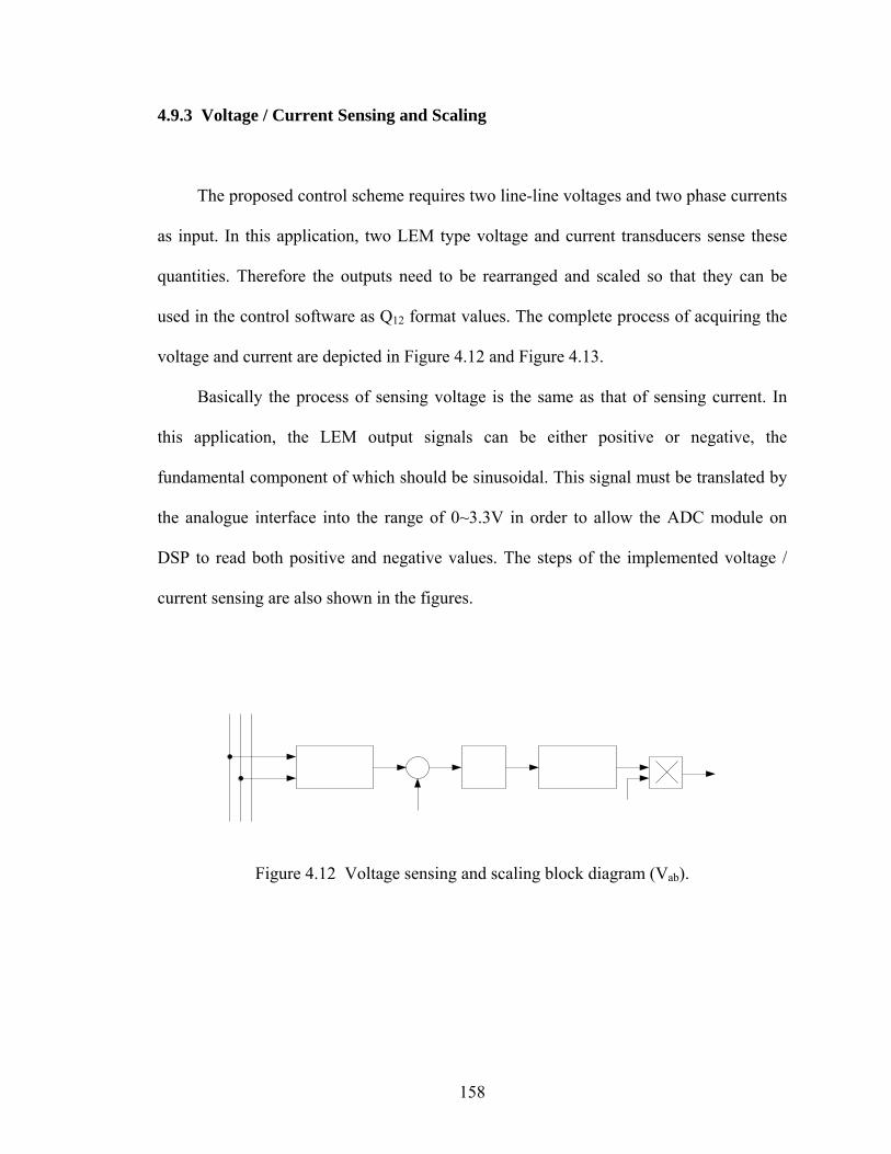
158

4.9.3 Voltage / Current Sensing and Scaling

The proposed control scheme requires two line-line voltages and two phase currents

as input. In this application, two LEM type voltage and current transducers sense these

quantities. Therefore the outputs need to be rearranged and scaled so that they can be

used in the control software as Q12 format values. The complete process of acquiring the

voltage and current are depicted in Figure 4.12 and Figure 4.13.

Basically the process of sensing voltage is the same as that of sensing current. In

this application, the LEM output signals can be either positive or negative, the

fundamental component of which should be sinusoidal. This signal must be translated by

the analogue interface into the range of 0~3.3V in order to allow the ADC module on

DSP to read both positive and negative values. The steps of the implemented voltage /

current sensing are also shown in the figures.

Figure 4.12 Voltage sensing and scaling block diagram (Vab).

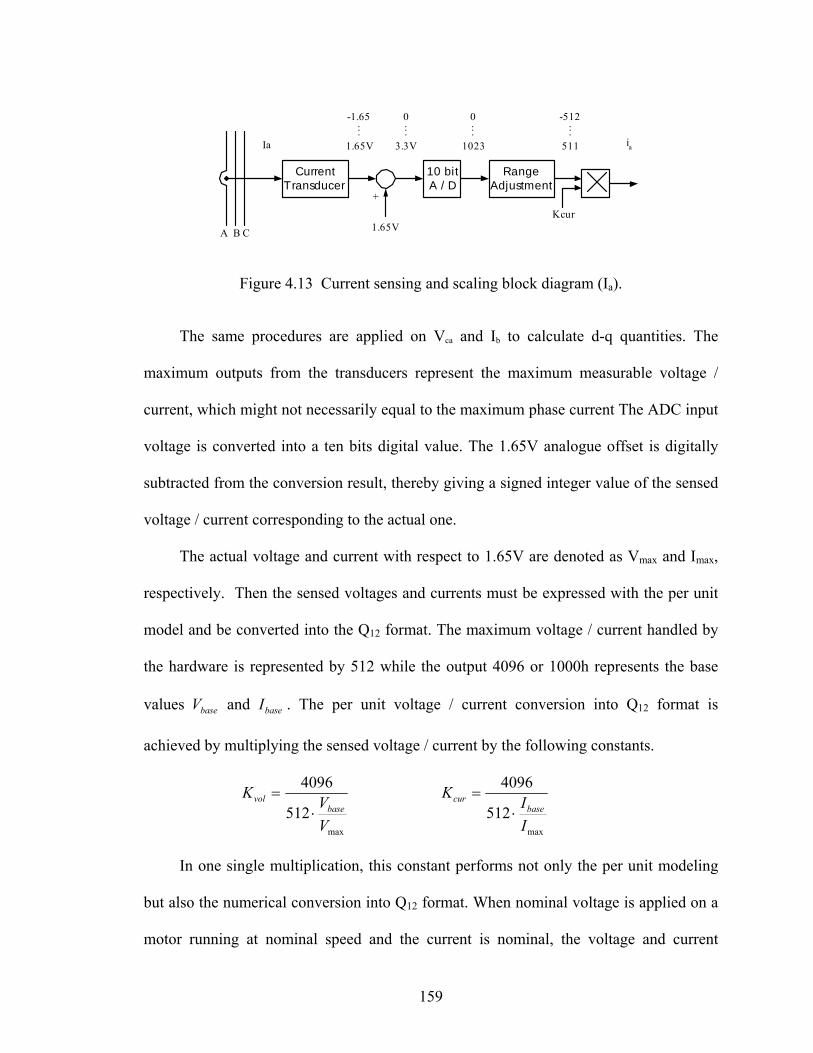
159

A B C

Ia

CurrentTransducer

10 bitA / D

RangeAdjustment

3.3V

+

1.65V

0...

1.65V

-1.65...

1023

0...

511

-512...

Kcur

ia

Figure 4.13 Current sensing and scaling block diagram (Ia).

The same procedures are applied on Vca and Ib to calculate d-q quantities. The

maximum outputs from the transducers represent the maximum measurable voltage /

current, which might not necessarily equal to the maximum phase current The ADC input

voltage is converted into a ten bits digital value. The 1.65V analogue offset is digitally

subtracted from the conversion result, thereby giving a signed integer value of the sensed

voltage / current corresponding to the actual one.

The actual voltage and current with respect to 1.65V are denoted as Vmax and Imax,

respectively. Then the sensed voltages and currents must be expressed with the per unit

model and be converted into the Q12 format. The maximum voltage / current handled by

the hardware is represented by 512 while the output 4096 or 1000h represents the base

values baseV and baseI . The per unit voltage / current conversion into Q12 format is

achieved by multiplying the sensed voltage / current by the following constants.

max

512

4096

VVK

basevol

⋅=

max

512

4096

IIK

basecur

⋅=

In one single multiplication, this constant performs not only the per unit modeling

but also the numerical conversion into Q12 format. When nominal voltage is applied on a

motor running at nominal speed and the current is nominal, the voltage and current

160

sensing and scaling block output is 1000h, which is equivalent to 1 in per unit. In this

implementation, the maximum measurable voltage and current are V 86.153max =V and

A 5.16max =I . So the constant values are

8Q06DA8523.6

86.15363.179512

4096 hKvol ⇔=⋅

=

8Q18905627.24

374.55.16512

4096 hKcur ⇔=⋅

=

Apparently curK is outside of the Q12 format range. The appropriate format to

accommodate this constant is Q8 format, which means that eight highest bits are

dedicated to the integer part and eight lowest bits are dedicated to the fractional part. The

corresponding resolution of Q8 is 0.00390625. The same data format is applied for volK .

4.9.4 Speed Sensing and Scaling

A 4096 pulse absolute encoder is used to measure the rotor speed in this induction

motor drive. Twelve digital I/O ports of the DSP TMS320LF2407 are occupied for

reading the output of the encoder. Generally, the mechanical time constant is much lower

than the electrical one. The speed regulation loop frequency might be lower than the

current loop frequency and it can be achieved by means of a software counter. This

counter takes the clock of PWM interrupt as the input and the speed is calculated every

250 PWM cycles.

161

Figure 4.14 Speed sensing and scaling block diagram.

Assuming that pn is the number of encoder pulses in 250 periods when the motor

runs at the nominal speed, a software constant speedK should be chosen as follows to let

the speed feedback be transformed into the Q12 format, which can be used directly in the

control scheme.

hnK pspeed 1000=⋅

The nominal speed of current motor drive is 1800 rpm and the switching frequency

of PWM is 10kHz. Then pn and speedK can be calculated as follows.

8

4

Q14A3334.130724096

307210250409660

1800

hK

n

speed

p

⇔==

=⋅⋅⋅= −

4.9.5 Slip Estimation

The slip calculation is shown in (4.12), in which qsI can be directly calculated from

the measured currents. The dynamic equation for drλ can be achieved by considering

(4.11) and (4.13) simultaneously and eliminating drI .

162

( )

drr

qsmslip

dsmdrr

TIL

ILpT

λω

λ

=

=⋅+1 (4.103)

And the rotor flux speed in per unit is just the sum of n and slipω .

basedrr

qsm

baseslips T

ILnnf

ωλωω 11

⋅+=⋅+= (4.104)

The integration of this speed gives the rotor flux position. The above equations can

be discretized as follows.

( )

1

1

1

11

+

+

+

⋅+=

−+=

+

k

k

k

kkkk

dr

qsm

baserks

drdsmr

drdr

ILT

nf

ILTT

λω

λλλ

(4.105)

The rotor flux is calculated during the slip estimation, which provides the

alternative way different with the application of LPF. Once the rotor flux speed has been

calculated, the necessary rotor flux position is computed by the integration formula.

Tf baseskk kωθθ ⋅+=+1 (4.106)

As the rotor flux position rang is 0~ π2 , 16 bits integer values have been used to

achieve the maximum resolution. The latter part of (4.103) is the angle variation within

one sample period. At nominal operation ( hfs 1000= ), the angle variation Tbaseω is

equal to 0.0377 rad. In one electrical revolution performed at nominal speed, there are

166.66 increments of the rotor flux position. Let K be the constant that converts the

0~ π2 range into the 0~65535 range. Then K is calculated as follows.

skk fK

K

⋅+=

==

+ θθ 1

22.39366.166

65536 (4.107)

163

4.9.6 Program Flowchart

The program flowchart of DSP implementation is shown in Figure 4.15.

Start

System configuration

Initialize peripherals:I/O pins, ADC

GP TimersPWM

Int control

Initialize variablesReset flags

Clear pending intsEnable interruptEnable GP Time

Determine Ids* through PI

Reset watchdog

End

PWM ISR

Read encoder outputsCalculate speed

Return

Calculate rotor flux

Transform to synchronousreference frame

Determine Iqs* through PI

Calculate the slip andsynchronous speed

Integrate to get phaseangle THETA

Obtain SIN(THETA) andCOS(THETA)

Sample stator voltagesand currents

Clarke transformation toget Vd, Vq and Id, Iq

Calculate stator flux byLow Pass Filter

( )∫ −= qdssqdsqds IRVλ

qdsqds I,λ

( )qdsqdsm

rqdr IL

LL

σλλ −=

Determine through PICalculate Vds*

Determine through PICalculate Vqs*

Transform to stationaryreference frame

Determine sector of Uout

Calculate Ta, Tb

Determine togglingsequence

Load compare registers

Enable interrupt

dsσ

qsσ

Figure 4.15 Program flowchart.

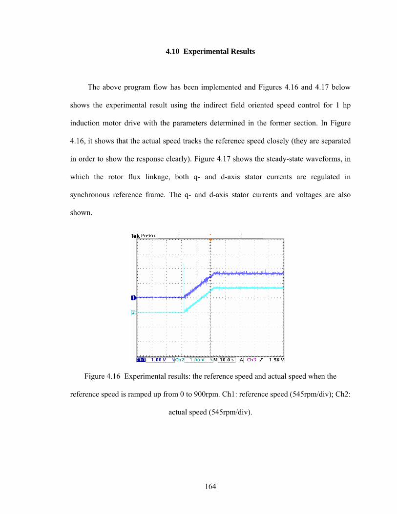
164

4.10 Experimental Results

The above program flow has been implemented and Figures 4.16 and 4.17 below

shows the experimental result using the indirect field oriented speed control for 1 hp

induction motor drive with the parameters determined in the former section. In Figure

4.16, it shows that the actual speed tracks the reference speed closely (they are separated

in order to show the response clearly). Figure 4.17 shows the steady-state waveforms, in

which the rotor flux linkage, both q- and d-axis stator currents are regulated in

synchronous reference frame. The q- and d-axis stator currents and voltages are also

shown.

Figure 4.16 Experimental results: the reference speed and actual speed when the

reference speed is ramped up from 0 to 900rpm. Ch1: reference speed (545rpm/div); Ch2:

actual speed (545rpm/div).

165

Figure 4.17a Experimental results at steady state. (a) Reference and actual d-axis rotor

flux linkages (0.6Wb/div); (b) reference q-axis stator currents (-1.65V, 3A/div); (c)

reference d-axis stator current (-1.65V, 3A/div).

(a) (b) (c)

166

Figure 4.17b Experimental results at steady state. (a) Q- and d-axis stator current in

stationary reference frame (6A/div); (b) q- and d-axis stator voltages in stationary

reference frame (50V/div).

Sometimes the induction machine is required to operate in both rotating directions,

clockwise and counter-clockwise. Such kind of operation has been verified through

experiments by changing the reference speed between -300rpm and 300rpm as shown in

Figure 4.18. The actual speed tracks the reference speed very well all the time.

(a) (b)

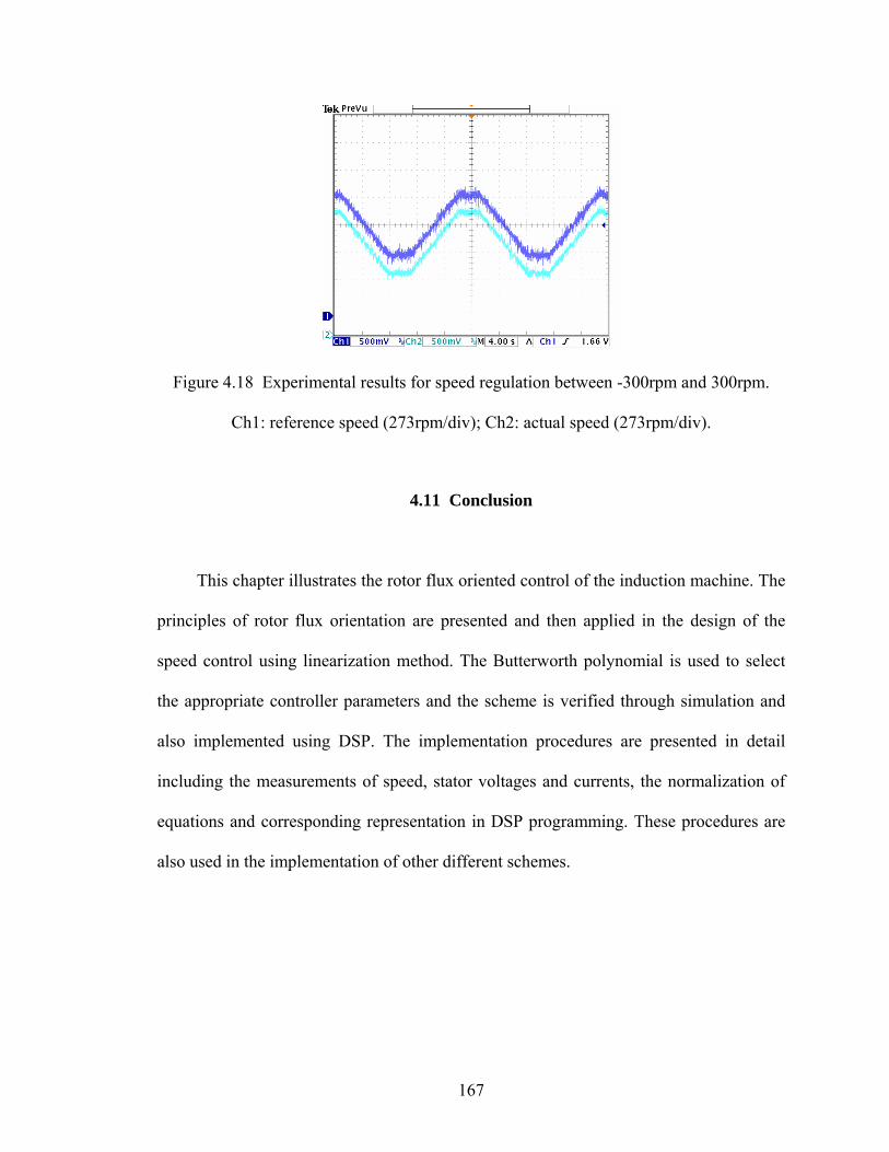
167

Figure 4.18 Experimental results for speed regulation between -300rpm and 300rpm.

Ch1: reference speed (273rpm/div); Ch2: actual speed (273rpm/div).

4.11 Conclusion

This chapter illustrates the rotor flux oriented control of the induction machine. The

principles of rotor flux orientation are presented and then applied in the design of the

speed control using linearization method. The Butterworth polynomial is used to select

the appropriate controller parameters and the scheme is verified through simulation and

also implemented using DSP. The implementation procedures are presented in detail

including the measurements of speed, stator voltages and currents, the normalization of

equations and corresponding representation in DSP programming. These procedures are

also used in the implementation of other different schemes.

168

CHAPTER 5

EFFICIENCY OPTIMIZING CONTROL OF INDUCTION MOTOR USING

NATURAL VARIABLES

5.1 Introduction

As mentioned in Chapter 1, the efficiency improvement of induction machines is

receiving more and more attentions since they are the greatest consumer of electric

power. A lot of energy will be saved even if the total efficiency of the induction machine

can be improved for just a little bit. Once the induction machine is manufactured, some of

the losses are not controllable including the some mechanical, electrical and stray losses.

However, the overall system losses of the induction machine can be minimized since the

resistive and core losses are depending upon the operating conditions. For example, the

induction machine can be operated at different flux level while the net output power is

maintained the same. Apparently the sum of the resistive and core losses is different

under the operation at different flux level. The study of the copper and core loss

components reveals that their trends conflict – when the core loss increases, the copper

loss tends to decrease. However, for a given load torque, there is an air-gap flux density

at which the total loss is minimized. Hence, electrical loss minimization process

ultimately comes down to the selection of the appropriate air-gap flux density. Since the

air-gap flux density must be variable when the load is changing, control schemes in

which the (rotor, air-gap) flux linkage is constant will yield sub-optimal efficiency

operation especially when the load is light.

169

This chapter presents an approach of simultaneously optimizing the efficiency of

induction motor drives and selecting flux linkage reference through the minimization of

the copper and core losses while ensuring high dynamic performance. The induction

machine model which accounts for the varying core loss resistance and saturation

dependent magnetizing inductance, uses natural variables, which are reference frame

independent quantities, as state variables – square of total rotor flux, active torque,

reactive torques, which is corresponding to the reactive power and rotor speed. The

inverter driving the motor is under pulse-width modulation and is voltage controlled.

Utilization of the nonlinear geometric control methodology of input-output linearization

with decoupling facility permits the implementation of the control in the stationary

reference frame. This approach eliminates the need of synchronous reference

transformation and flux alignment required in classical vector control schemes. The

efficiency optimizing formulation yields a reference rotor flux which ensures minimum

loss resulting in an improved efficiency of the drive system. The proposed scheme and its

advantages are demonstrated both by computer simulations and some experimental

results for induction motor speed control.

5.2 Induction Motor Model with Core Loss

The stationary reference frame q-d equivalent circuit of the induction machine is

shown in Figure 5.1 in which the core loss is represented by a core loss resistance. The

voltage equations for the induction motor in the arbitrary reference frame rotating at the

speed ω are given as:

170

qrrdrdrr

drrqrqrr

qsdsdssds

dsqsqssqs

pIr

pIr

pIrV

pIrV

λωωλ

λωωλ

ωλλ

ωλλ

)(0

)(0

−−+=

−++=

−+=

++=

(5.1)

where

drmdssds

qrmqssqs

ILIL

ILIL

+=

+='

'

λ

λ,

'

'

dsmdrrdr

qsmqrrqr

ILIL

ILIL

+=

+=

λ

λ.

Define r

ms L

LLL

2

−=σ and c

s

rr

k += 1 , the stator voltage equations can be expressed

in terms of '' , dsqs II and drqr λλ , as follows.

dsωλlsLsr

qsVqsI

mL

+ -'qsI

cr cqI

lrL ( ) drr λωω −

- +rr

qrIqrV

(a)

qsωλlsLsr

dsV dsI

- +'dsI

cr cdImL

lrL ( ) qrr λωω −

+ -rr

drIdrV

(b)


resistance. (a) Q-axis; (b) d-axis.

171

qrrdrdrr

drrqrqrr

dsqrr

mrdrds

ds

qsdrr

mrqrqs

qs

pIr

pIr

pILLL

crIk

V

pILLL

crIk

V

λωλ

λωλ

λω

λ

λω

λ

σ

σ

++=

−+=

+−−=

++−=

0

0

''

''

(5.2)

where

2

2

r

mrs

LLr

kr

r += , 2r

mr

LLr

c = .

Vqs and Vds are the stator qd-axis voltages. Iqs' and Ids

' are the q- and d-axis torque

effective currents. Iqr and Idr are the q- and d-axis rotor currents. λqr and λdr are the rotor

flux linkages. rs, rr, and rc are the stator, rotor resistance and stator core loss resistance,

which accounts for the stator core loss. Ls, Lr, and Lm are stator self-inductance, rotor self-

inductance, and mutual inductance. ωr is the electrical rotor speed and p represents the

derivative.

Equations (5.1-2) contain the mutual inductance and the core loss resistance that are

changing with the flux linkage. These changes are accounted for in both computer

simulations and experimental implementation of the controllers by updating them as the

stator flux linkage varies. These parameter changes for a 1 hp machine are shown in

Figure 3.6, in which the measured mutual inductance and core resistance are plotted as a

function of the stator flux linkage.

172

5.3 Natural Variable Model and Total Loss Minimization

The variables of the natural variable model of the induction machine are chosen as

the developed electromagnetic torque eT , the developed reactive torque rT , the rotor

speed rω , and the square of the magnitude of the rotor flux linkage rrλ . These variables

are the same in all reference frames or independent of the selected reference frame. Then

these natural variables are expressed in terms of the axis currents and flux linkages as:

( )( )

22

''

''

drqrrr

qsqrdsdrtr

dsqrqsdrte

IIkT

IIkT

λλλ

λλ

λλ

+=

+=

−=

(5.3)

where r

mt L

PLk4

3= and P is the poles of the machine.

The losses existing in the induction machine include many different kinds such as

the stator and rotor copper losses, stator and rotor core losses, mechanical loss, and stray

loss. Generally these losses vary under different operating conditions. However, under

the certain operating condition, most of the losses are not controllable except the stator

and rotor copper and core losses. The stator and rotor copper losses are essentially

determined by the corresponding resistances and currents while the stator core loss can be

calculated from the core loss resistance and the currents flowing through.

( ) ( ) ( )222222

23

23

23

cdcqcdrqrrdsqssL IIrIIrIIrP +++++= (5.4)

173

Since now the effective torque currents are used, the stator and rotor currents and

the currents flowing through the core loss resistance can be expressed in terms of Iqs' , Ids

'

, λqr, and λdr . And eventually the total loss can be rewritten using the natural variables

defined in (5.3) as

( )

er

mre

ctr

cre

rc

m

t

rrrrc

m

r

r

crr

re

c

e

tL

TLL

rLcrkkTc

rkrc

LrLkL

k

LrkL

Lr

rkcTT

rLrk

rk

P

⎟⎟⎠

⎞⎜⎜⎝

⎛++⎟⎟

⎠

⎞⎜⎜⎝

⎛−−+

⎟⎟⎠

⎞⎜⎜⎝

⎛+++

+⎥⎦

⎤⎢⎣

⎡ ++=

ωωωω

λωλ

ω

σσ

σ

33

23

23 2

2

2

2

222222

2

(5.5)

where 2

2

r

mrs

LLr

kr

r += , 2r

mr

LLr

c = .

The total electrical loss is to be minimized when the motor is subject to an

operating load torque, *ee TT = . Either rrλ or rT can be chosen as the control variable to

form the loss minimization function γ . Both rrλ and rT cannot be used as the control

variables at the same time for the loss minimization. This can be examined from the

derivative of the magnitude square of the rotor flux linkages. Apparently the derivative of

rrλ is zero at steady state, which means that rrλ and rT are dependent if all the machine

parameters are assumed constants.

rrt

mrrr

r

rrr T

LkLr

Lrp

22+−= λλ (5.6)

The electric loss is minimized when any of the two determinants in (5.7-8) is

identically equal to zero. These two determinants are not zero in general while they are

supposed to be zero when the total electrical loss is minimized.

174

( )rerrerr

L

rr

L

e

L

rr

e

e

e

TfPP

TP

TTT

ωωλγλ

λ

λγ ,,,0 1=⇒=∂∂

=

∂∂

∂∂

∂∂

∂∂

= (5.7)

( )rerer

L

r

L

e

L

r

e

e

e

TTfTP

TP

TP

TT

TT

ωωγγ ,,,0 2 =⇒=∂∂

=

∂∂

∂∂

∂∂

∂∂

= (5.8)

Based on the above analysis, these two formulations give out the same results at the

steady state. In the case of (5.7), it can be expressed in terms of the natural variables as

( )

⎟⎟⎠

⎞⎜⎜⎝

⎛−−+⎟⎟

⎠

⎞⎜⎜⎝

⎛+++

⎟⎟⎠

⎞⎜⎜⎝

⎛ +−⎥

⎦

⎤⎢⎣

⎡ ++=

cr

krcLrLkL

LLrkL

Lr

rkc

TTLkT

rLrkr

k

cre

rc

m

mr

rc

m

r

r

c

rr

re

m

t

rr

r

c

e

t

ωωω

λλωγ

σ

σ

323

223

22

2

2

2

2

22222

2

(5.9)

The total electric loss is minimized when 0=γ under steady-state operation. Then

the corresponding optimum rotor flux is calculated as

( )

RL

cr

krcLrLkL

LLrkL

Lr

rkc

TTRk

mcre

rc

m

mr

rc

m

r

r

c

ret

rr

22

2

2

2

2

222

3323

23

+⎟⎟⎠

⎞⎜⎜⎝

⎛−−+⎟⎟

⎠

⎞⎜⎜⎝

⎛++

+=

ωωωλ

σ

(5.10)

where

( )c

e

rLrkrR

222σω+

+= .

175

5.4 Formulation of Control Scheme

The total loss minimization is achieved through appropriate command of the q-d

axis machine voltages by closed-loop controllers using a voltage controlled voltage

source inverter. Since the model of the machine is nonlinear and coupled, the principles

of nonlinear control of the input-output linearization with decoupling are used to remove

the nonlinearity and coupled terms thereby enabling classical linear system control

methodology to be used to determine both the constant gain parameters and the structure

of the controllers [5.11-5.12]. This is possible since the input-output linearization and

decoupling strategy ensures linear relationships between the input control variables and

the controlled variables with each output-input pair decoupled from each other.

Input-output linearization is a three-step process: (a) differentiate a controlled

variable until an input variable appears, (b) choose the input variable to cancel nonlinear

terms and guarantee tracking convergence, and (c) study the stability of the internal

dynamics. The total number of differentiations for all controlled variables is called the

relative order r, while the internal dynamics are composed of n-r states (n is the total

number of the system dynamic states). When operations (a-c) are performed on the motor

model equations (5.3), the resulting equations are linearized, decoupled with no internal

dynamics and input-output linearizable. Hence any realistic dynamics can be imposed by

means of linear controllers.

1mkL

kLLLk

TTLLLr

kLr

pT trrr

r

mtrre

r

srse

σσσσ

λωω +−−⎟⎟⎠

⎞⎜⎜⎝

⎛+−= (5.11)

( )Ler TTJ

Pp −=2

ω (5.12)

176

22

22

mkL

kLLLrk

TTT

kLLr

TLLLr

kLr

pT

trr

r

mrt

errr

re

tr

mrr

r

srsr

σσ

σσ

λ

ωλ

++

++

+⎟⎟⎠

⎞⎜⎜⎝

⎛+−=

(5.13)

rrt

mrrr

r

rrr T

LkLr

Lrp

22+−= λλ (5.14)

where

dsdrqsqr

dsqrqsdr

VVm

VVm

λλ

λλ

+=

−=

2

1 (5.15)

The quantities 1m and 2m are calculated using the outputs of the controllers for eT

and rT . Then the voltages commands are calculated by solving (5.15).

rr

qrdrds

rr

qrdrqs

mmV

mmV

λλλ

λλλ

12

21

−=

+=

(5.16)

Popular PI controllers are applied for the control of rerr TT ,,λ , and rω .

pKKK i

pλ

λλ += , p

KKK r

rr

iTpTT += ,

pKKK i

pω

ωω += , p

KKK e

ee

iTpTT +=

Their corresponding transfer functions are derived as follows.

( )rrrrrrr

rrr K

Lr

p λλλλσ λλ −=+= *2

( )rrTrr

srsrT TTKT

LLLr

kLr

pTrr

−=⎟⎟⎠

⎞⎜⎜⎝

⎛++= *

σσ

σ (5.17)

177

( )[ ]rrr KpJ

Pp ωωω ω −⋅= *2

2, ( )rre KT ωωω −= *

( )eeTer

srseT TTKT

LLLr

kLr

pTee

−=⎟⎟⎠

⎞⎜⎜⎝

⎛++= *

σσ

σ

The controller parameters are determined from the transfer functions by tuning the

denominators to be Butterworth polynomial compliant, which is to optimize the closed-

loop eigen-values to be uniformly located in the left half plane on the circle of the

resonant frequency. Butterworth polynomial for a transfer function with a second order

polynomial is given by

02 200

2 =++ ωωpp (5.18)

Comparing the coefficients of the denominators of the transfer functions obtained

from (5.17) and (5.18) gives the controllers’ gains for a chosen resonant frequency 0ω .

The selection of the resonant frequency is such as to ensure the closed-loop transfer

functions of the controlled variables have minimum-phase characteristics [5.13]. The

controller structure for the motor speed control is shown in Figure 5.2.

The rotor position, motor phase currents and phase voltages are measured to

estimate the natural variables and the rotor flux linkages which are required for the

control implementation. Only the stationary reference frame transformation is required in

the estimation of the natural variables.

178

∗rT

∗rω

Transformation

BA

CAAB

IIVV

,,

AB

C

*dsV

Inverter

*qsV

rTσ

eTσ

dsqs VV ,

∗rrλ

+

-rrλ

λK

-

+

rω

∗eT

ωK

dsqs λλ , ( )∫ − qdssqds IrVEq. (5.3)

+

-rT

rTK

-eT

eTK

Space

Vector

PWM+

dsqs II ,Eq. (5.3)

Eq. (5.3)

Eq.(5.9)

Eq.(5.11)

1m

2m

Eq.(5.14)

Eq.(5.8)

rω

mr

rt

LrLk

2reeT ωω ,,

Motor

Figure 5.2 Control scheme for induction motor with electrical loss minimization strategy.

5.5 Speed Estimation

In the case of speed sensorless control, the rotor speed needs to be estimated from

the measured quantities. There are different kinds of methods that can be used for the

rotor speed estimation. Since the reference frame independent state variables are used, the

first choice is to use the same state variables to estimate the rotor speed.

5.5.1 Using Imaginary Power

The first method is tried using the imaginary power. From the definition of the

natural variables, the reactive power of the induction motor can be found in terms of the

state variables as

( )rrree TTfQ λω ,,,= (5.19)

Since slipre ωωω += and the slip frequency can be calculated from the steady state

equations as

179

rr

e

tr

mrslip

TKLLr

λω ⋅= (5.20)

Then the rotor speed can be estimated using (5.19-20) as

rrt

mr

rrt

re

ert

mr

rrt

re

rr

e

tr

mr

r

TLK

LrK

TTL

TLKLr

KTTLT

KLLrQ

⋅++

⋅

⋅−+

⋅⋅⋅−−=

λ

λλω

σ

σ

2

22

22

22

32

(5.21)

This method is simulated and the procedures of sensorless scheme for both

simulation and implementation are similar. First of all, the control scheme with speed

regulation using speed sensor should work properly. Then the speed is estimated while

the motor is still running using the speed from the speed sensor as feedback. Once the

estimated speed is getting very close to the actual speed, it can then be used as feedback

to see if it works. Of course, the simulation has to be done first and then it can be

implemented after the simulation works. In this simulation, the reference rotor speed is

ramped up from 0 to 150 rad/s. The rotor speed is estimated very well when the actual

rotor speed is used as the feedback. However, there are big oscillations in the actual rotor

speed while the estimated rotor speed is used as the feedback. And the developed electric

torque also has big oscillations, which is not desirable.

5.5.2 Using Rotor Voltage Equations

It is known that the rotor speed information can be extracted from the rotor voltage

equations, which can be classified into category of using the motor back EMF. The two

rotor voltage equations are

180

(a) (b)

(c)

Figure 5.3 Simulation of the rotor speed estimation including reactive power. (a)

Reference and actual rotor speeds; (b) Reference and actual rotor speeds; (c) Developed

electric torque.

( )( ) qrredrdrr

drreqrqrr

jpIr

jpIr

λωωλ

λωωλ

−−+=

−++=

0

0 (5.22)

The rotor currents are not directly measurable and can be expressed in terms of the

rotor flux linkages and stator currents as

181

( )

( )dsmdrr

dr

qsmqrr

qr

ILL

I

ILL

I

−⋅=

−⋅=

λ

λ

1

1

(5.23)

The rotor voltage equations change to

qrredrdsr

mrdr

r

r

drreqrqsr

mrqr

r

r

pILLr

Lr

pILLr

Lr

λωωλλ

λωωλλ

)(0

)(0

−−+−=

−++−= (5.24)

When 0=eω , there equations are simplified in the stationary reference frame as

qrrdrdsr

mrdr

r

r

drrqrqsr

mrqr

r

r

pILLr

Lr

pILLr

Lr

λωλλ

λωλλ

++−=

−+−=

0

0 (5.25)

Either one of these two equations can be used to estimate the rotor speed when the

rotor flux linkages are known. Since both qrλ and drλ are AC signals, the estimation will

not work properly when the flux linkage as the coefficient of rω is zero. One of the

solutions is to use both equations alternatively by finding the bigger rotor flux linkage.

That is

If qrdr λλ >

drdrqsr

mrqr

r

rqrr XI

LLr

Lrp λλλλω =⎟⎟

⎠

⎞⎜⎜⎝

⎛−+=ˆ (5.26)

Else

qrqrdsr

mrdr

r

rdrr YI

LLr

Lrp λλλλω =⎟⎟

⎠

⎞⎜⎜⎝

⎛+−−=ˆ (5.27)

182

The simulation results are shown in Figure 5.4. It is seen that the rotor speed is

regulated when the estimated speed is used as the feedback. The only problem is that the

estimated rotor speed is oscillating around the actual speed. This kind of oscillation exists

all the time such that it is not a good estimation.

(a) (b)


Reference and estimated rotor speeds; (b) reference and estimated rotor speeds.

183

5.5.3 Using Rotor Voltage Equations (modified)

Instead of using only one of the two rotor voltage equations at a time, it is possible

to use both of them at the same time in order to eliminate the oscillations. That is using

the square root of the sum of squares of the estimated speed from these two equations.

The rotor speed can be estimated from

qrqrdsr

mrdr

r

rdrr

drdrqsr

mrqr

r

rqrr

YILLr

Lr

p

XILLr

Lr

p

λλλλω

λλλλω

=⎟⎟⎠

⎞⎜⎜⎝

⎛+−−=

=⎟⎟⎠

⎞⎜⎜⎝

⎛−+=

ˆ

ˆ

(5.28)

And the final rotor speed is re-calculated from (5.28) as

22

22

qrdrr

YXλλ

ω++

= (5.29)

The simulation results are shown in Figure 5.5. It is seen that the rotor speed is

regulated very well when the estimated speed is used as the feedback. The steady state

error between the actual rotor speed and the estimated rotor speed is very small. And the

estimated rotor speed is constant at the steady state, which is good characteristic. It means

that the error for the estimation can be compensated even if this error is big.

184

Wr

Wr_est


Reference and estimated rotor speeds; (b) reference and estimated rotor speeds.

(a) (b)

185


Figure 5.6 gives the no-load starting transient of an experimental 1 hp induction

machine whose parameters are shown in Figure 3.6 and Table 3.1. The reference speed is

ramped from zero to 300 rad/sec while seeking to minimize the total electrical loss. The

simulation results show that the rotor flux linkage quickly builds up and maintains an

almost constant rated value and becomes small at steady-state. The total loss reduces as

the developed torque becomes zero, in which case the ideal stator current is zero and

hence the copper loss is zero.

Figure 5.6 Speed regulation and loss minimization for motor starting from zero speed to

300 rad/sec. (a) Developed torque; (b) reference and actual rotor speeds; (c) rotor flux

linkage; (d) total electric loss.

(a) (b) (c) (d)

186

In Figure 5.7, the speed is maintained at 300 rad/sec, but the load torque is

changing. As expected, the rotor flux responds to the changing load demand resulting in

the minimization of the losses. As the load demand decreases, the optimum rotor flux

linkage also decreases resulting in a lower loss. In Figure 5.8, the rotor speed is changed

with time and it is seen that both the rotor flux linkage and the loss seeks the minimum

level. The speed change with constant slope is basically working as putting a constant

load to the induction motor. In these simulations, the rotor flux linkage is limited below

the rated value, the square of which is about 0.2 wb2.

Figures 5.6-8 demonstrate the possibilities that this control scheme presents –

changing load or reference speed commands appropriate flux linkage to minimize the

electric loss while giving high performance speed control. Figure 5.9 shows the changing

speed between both positive and negative directions. It appears that the motor speed is

still regulated very well under such operating condition.

The proposed speed estimation method has already been simulated for the speed

control in the above section. Figure 5.10 shows the speed response for a constant flux

reference when the load is under step change. It is seen that the estimated speed is almost

identical to the actual speed. It verifies the effectiveness of the proposed sensorless

approach.

187

Figure 5.7 Speed regulation and loss minimization for changing load torque. (a)

Developed torque; (b) actual and command rotor speed; (c) square of rotor flux linkage;

(d) total electric loss.

Figure 5.8 Speed regulation and loss minimization for changing rotor speed. (a)

Developed torque; (b) actual and command rotor speed; (c) square of rotor flux linkage;

(d) total electric loss.

(a) (b) (c) (d)

(a) (b) (c) (d)

188

Figure 5.9 Response to the speed change after steady state. (a) Reference speed and

actual speeds; (b) electrical torque.

Figure 5.10 Actual / estimated rotor speed corresponding to load change. (a) Reference

and estimated speeds; (b) electric torque.

(a) (b)

(a) (b)

189


The proposed control scheme using natural variables and the modified rotor speed

estimation have been implemented using TI DSP TMS320LF2407 EVM board. Figure

5.11 below shows the no-load speed response of the motor when it is ramped from zero

speed to 820 rpm. While the reference speed tracks the actual closely, it is observed that

the flux linkage is also changing and reducing as the steady-state no-load speed is

approached which is what is observed in the simulation results. In Figure 5.12, reference

speed is decreased and increased and the actual speed tracks it very well. Also observed

is the fact that the rotor flux linkage changes with a change in the reference speed.


(545rpm/div); Ch2: actual rotor speed (545rpm/div); Ch3: square of rotor flux linkage

(0.1Wb2/div); Ch4: phase A current (6A/div).

190

Figure 5.12 Speed regulation and loss minimization for changing rotor speed from zero

to 900-600 rpm. Ch1: reference rotor speed (545rpm/div); Ch2: actual rotor speed

(545rpm/div); Ch3: square of rotor flux linkage (0.1Wb2/div); Ch4: phase A current

(6A/div).

In the experiments, the rotor speed is estimated using both rotor voltage equations

and the actual speed measured from the absolute encoder is used as the feedback first to

check whether the estimated rotor speed is close to the actual value. If they are very

close, the estimated speed is then used as the feedback. The stator and rotor flux linkages

are estimated using low pass filters with magnitude and phase error compensations

illustrated in Chapter 4.

In the estimation of rotor flux linkages, the derivatives of the rotor flux linkages

need to be calculated first. Generally the digital calculation of derivatives is not desired

especially when the signals are AC signals. Since the rotor flux linkages are calculated

from the stator flux linkages and the stator currents, one of the ways of getting better

results is to use the measured quantities directly. Hence the derivatives of rotor flux

191

linkages can be expressed in terms of the stator voltages, stator currents and the

derivatives of stator currents, which are expected to give better results since the stator

currents are measured directly while the rotor fluxes are the estimated quantities using

stator currents.

( )

( ) dsr

mrdr

r

rdsdssds

m

r

qsr

mrqr

r

rqsqssqs

m

r

ILLr

LrpILIrV

LLY

ILLr

LrpILIrV

LLX

+−−−⋅−=

−+−−⋅=

λ

λ

σ

σ

(5.30)

And the derivatives of stator currents are calculated as

( ) ( )

( ) ( )s

dsdsds

s

qsqsqs

TkIkIpI

TkIkI

pI

−+=

−+=

1

1

(5.31)

where Ts is the sampling period, which is also the switching period in the DSP code. This

method of calculating the derivatives of the stator currents is tested first by using the

actual rotor speed measured from the absolute encoder. The actual rotor speed tracks the

reference speed very well. But there are big spikes in the estimated rotor speed as shown

in Figure 5.13 when the reference rotor speed is ramped up from 0 to 600rpm. This is the

normal case when the derivatives are calculated using (5.31).

192

Figure 5.13 Actual rotor speed and estimated rotor speed (using actual speed as


(545rpm/div).

Then the estimation of the rotor speed without calculating the derivatives of the

stator currents is tested to check if those spikes come from the calculation of derivatives.

The speed waveforms are shown in Figure 5.14 when the actual rotor speed is used as the

feedback also. It is seen that the estimated rotor speed has a much better waveform than

the precious case. However, the steady state value is much lower than the reference rotor

speed. In this particular case, the reference rotor speed is 600rpm and the actual rotor

speed is 597rpm. But the estimated rotor speed is only 548 rpm, which means that the

calculation of the derivatives of the stator currents cannot be neglected.

193

Figure 5.14 Actual rotor speed, estimated rotor speed and filtered estimated rotor speed (

without calculating the derivatives, using actual speed as feedback). Ch2: actual rotor

speed (545rpm/div); Ch3: estimated rotor speed (545rpm/div); Ch4: filtered estimated

rotor speed (545rpm/div).

In order to avoid the spikes in the estimated rotor speed due the calculations of the

derivatives of the stator currents, these derivatives are calculated every four sampling

periods. By this way, the noise introduced by (5.30) can greatly reduced.

( ) ( )

( ) ( )s

dsdsds

s

qsqsqs

TkIkIpI

TkIkI

pI

∗−−

=

∗

−−=

44

44

(5.32)

The speed waveforms are shown in Figure 5.15, in which the estimated speed is

very close to the actual speed. At the steady state, the actual speed is 597rpm and the

estimated one is 591rpm while the reference speed is 600rpm and the actual speed is used

as the feedback.

194

Figure 5.15 Actual rotor speed, estimated rotor speed and filtered estimated rotor speed

(calculating the derivatives every 4 sampling period, using actual speed as feedback).

Ch2: actual rotor speed (545rpm/div); Ch3: estimated rotor speed (545rpm/div); Ch4:

filtered estimated rotor speed (545rpm/div).

The next step is to use the estimated speed as the feedback signal. The speed

waveforms are shown in Figure 5.16 for a constant speed reference and in Figure 5.17 for

changing speed reference. It is seen that the estimated rotor speed is very close to the

actual speed, which means that the rotor speed is estimated successfully. The only

problem is that there are some oscillations in the estimated rotor speed and also in the

actual rotor speed. This test is done at almost no-load condition. The waveforms are

greatly improved when a light load is applied, as shown in Figure 5.18.

195



Ch1: reference speed (545rpm/div); Ch2: measured speed (545rpm/div); Ch4: estimated

speed (545rpm/div).



Ch1: reference speed (545rpm/div); Ch2: measured speed (545rpm/div); Ch4: estimated

speed (545rpm/div).

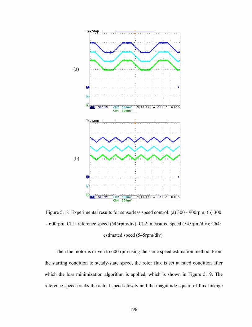
196

Figure 5.18 Experimental results for sensorless speed control. (a) 300 - 900rpm; (b) 300

- 600rpm. Ch1: reference speed (545rpm/div); Ch2: measured speed (545rpm/div); Ch4:

estimated speed (545rpm/div).

Then the motor is driven to 600 rpm using the same speed estimation method. From

the starting condition to steady-state speed, the rotor flux is set at rated condition after

which the loss minimization algorithm is applied, which is shown in Figure 5.19. The

reference speed tracks the actual speed closely and the magnitude square of flux linkage

(a) (b)

197

reduces after the loss minimization algorithm kicks in. There is however an initial

divergence between the actual and estimated speed at the starting condition when the

rotor flux linkage is kept constant. Finally, Figure 5.20 displays the changing rotor flux

linkage profile for the loaded motor under changing rotor speed condition. This graph

succinctly demonstrates how the optimum rotor flux linkage command is changing which

should consequently affect the loss in the machine – improving overall motor efficiency.


(545rpm/div); Ch2: actual rotor speed (545rpm/div); Ch3: square of rotor flux linkage

(0.1Wb2/div); Ch4: phase A current (6A/div).

198

Figure 5.20 Speed regulation ( 300 – 600 rpm) showing rotor flux variation. Ch1:

reference speed (273rpm/div); Ch2: estimated speed (273rpm/div); Ch3: rotor flux

linkage (0.1Wb2/div).

5.8 Loss Minimization Using a Controller for the Loss Minimization Function

In the above analysis, the optimum rotor flux is calculated from the loss

minimization function and then used in the control scheme. However, it is possible to

regulate the loss minimization function directly and the loss is minimized when the

function is regulated to be zero. The derivative of the loss minimization function is

calculated as

( ) γσλγ =++⋅−= CBA

kp

rrt22

12

3 (5.33)

where

199

( )

( )

( )errerc

rrrc

mre

mc

ret

rr

rerrr

r

mt

rerr

r

rt

mr

r

rss

ppLr

kLp

LrkL

pLr

kLC

TmTmkLk

TLr

TLLLk

B

TTT

LkLr

Lr

LL

Lr

A

ωωωωωωωω

ωλ

λ

σσ

σσ

σσ

+++=

++⎟⎟⎠

⎞⎜⎜⎝

⎛−−=

+⎥⎥⎦

⎤

⎢⎢⎣

⎡−⎟⎟

⎠

⎞⎜⎜⎝

⎛−+−=

336

2

2

2

2

2

21

22

Differentiating (5.9) and substituting (5.6), the rotor speed dynamics is given as

( ) errr pTKp =−= ωωω ω*2 (5.34)

A general controller ωK such as the IP controller is assumed in (5.12) for the speed

control loop and the corresponding transfer function is expressed in (5.35). The

application of IP controller ensures that the denominator is Butterworth polynomial

compliant and the there is no zero in the numerator.

212

1* KpKp

K

r

r

++=

ωω (5.35)

Similarly, for the loss function loop, a controller γK such as the PI controller is

used in (5.33) resulting in the following dynamics.

( ) γγ σγγγ =−⋅= *Kp (5.36)

The corresponding transfer function is given as

432

3* KpKp

K++

=γγ

(5.37)

The schemes for the speed and loss minimization controllers are shown in shown in

Figure 5.21.

200

+

-

+

-

*rω

rω

ikω ωσ

pk pω

+

-

+*γ

γ

pk iω γσ

pkω+

(a) Speed controller (b) Loss minimization controller

Figure 5.21 The structures of controllers.

The starred terms in (5.34-37) are the reference values which for γ* is set to

zero. The gain parameters of the PI and IP controllers are selected such that the

denominator of the transfer functions of control variables are tuned to be Butterworth

polynomial compliant also. Comparison of the coefficients of the denominators of the

transfer function (5.35, 5.37) with (5.18) gives the gain parameters for the controllers

for a chosen resonant frequency 0ω .

Substituting (5.36) into (5.33) and (5.11) into (5.34), the resulting linear

equations when solved gives m1 and m2 . From (5.16), the reference q-d voltages are

determined and become the inputs to the space-vector implementation algorithm for

the three-phase voltage source inverter driving the induction machine. Figure 5.22

schematically shows the overall block diagram for the drive system. The beauty of

this control scheme is its simplicity. Only two controllers are necessary for the speed

control and electrical loss minimization at the same time. However, the simulation of

this control scheme is not successful. The reduction of controllers might be the

reason, in which case the state variables are not regulated directly.

201

∗rω

Transformation

BA

CAAB

IIVV

,,

AB

C

*dsV

Inverter

*qsVeTσ

dsqs VV ,

-

+

rω

ωK

dsqs λλ , ( )∫ − qdssqds IrVEq. (5.3)

Space

Vector

PWM

dsqs II ,

Eq.(5.33)

Eq.(5.34)

( )21, mmf

1m

Eq.(5.16)

0* =γ

-

+

γ

rω

γK

rrre TT λ,,

Motor

Figure 5.22 Schematic diagram of the control algorithm.

5.9 Conclusion

This chapter presents an approach of optimizing the efficiency of induction motor

drives through minimizing the copper and core losses using geometric nonlinear control.

This is made possible by a definition of a loss function which when regulated delivers

minimum loss operation. The induction machine model accounts for the varying core loss

resistance and saturation dependent magnetizing inductance by updating them as the

stator flux linkage varies. In problem formulation, the model machine model uses natural

and reference frame independent quantities as state variables. Utilization of the nonlinear

geometric control methodology of input-output linearization with decoupling, permits the

implementation of the control in the stationary reference frame. This approach eliminates

the need of synchronous reference transformation and flux alignment required in classical

vector control schemes. The new efficiency optimizing formulation yields a reference

202

rotor flux which ensures minimum loss and yields an improved efficiency of the drive

system especially when driving part-load. The proposed control is validated by computer

simulation and some experimental results on a 1 hp induction machine.

203

CHAPTER 6

SPEED ESTIMATION FOR INDUCTION MOTORS USING FULL-ORDER

FLUX OBSERVERS

6.1 Introduction

Induction motors have been studied for a long time since they were widely used in

the industry. Speed control is quite common in most induction motor applications.

Traditionally the speed information of an induction motor is measured or calculated using

a rotor position or speed sensor. The research on the speed control of induction motors

has been moving to the sensorless control, which eliminates the need of installing speed

sensor in order to reduce the cost, or operate in special conditions.

Speed sensorless control is basically the algorithm of speed estimation that can infer

the required measurement from other more easily available measurements like voltages

and currents. The techniques that have been developed can be classified into three

categories, which have been described in Chapter 1. The full-order observer system is an

alternative method of the first category. It estimates the stator flux linkages or currents

and rotor flux linkages using the voltages applied to the motor and measured currents.

Then a particular error function can be chosen to estimate the rotor speed through some

controllers. Since there are two sets of currents, one is the set of measured or actual

currents and the other is the set of estimated currents, the torque equations corresponding

to the active and reactive power are preferred. The adaptive mechanism is established

when the rotor speed estimated from this error is used as the feedback. The estimated

204

rotor speed is equal to the actual speed when this error is minimized to be zero.

Apparently this method is a closed-loop estimation, which is different from the flux

estimation using the stator voltage equations.

From the review of the work on the full-order observers, some fundamental issues

have not been adequately addressed including the selection of observer and the speed

adaptation gains based on stability analysis. In this chapter, the full-order flux observer

and the speed adaptive mechanism are defined. The model is used to estimate the flux

linkages, stator currents and the rotor speed of an induction motor through an adaptive

mechanism. The observer gains are chosen using Butterworth polynomials to ensure

system stability. The transfer function between the estimated speed and actual speed is

derived in the synchronous reference frame based on the error analysis, which are used to

select appropriate PI controller parameters for the speed estimation that ensures operation

in the stable region. The D-decomposition method is applied to determine the stable and

unstable regions from the transfer function. The rotor flux oriented control including the

observer and adaptive speed estimation are designed to examine the proposed methods.

The controller parameters are determined from the corresponding transfer functions. The

whole system is simulated in both motoring and regenerating modes. It is shown that all

the controllers work properly and the rotor speed is regulated very well under different

load conditions, which validate the proposed method of designing full-order flux observer

and speed estimator.

205

6.2 Induction Machine Model

The analysis is based on the synchronous reference frame, the complex form is

adopted for all quantities in q-d axis to simplify the analysis as

drqrqdrdsqsqds

drqrqdrdsqsqds

drqrqdrdsqsqds

jj

jIIIjIII

jVVVjVVV

λλλλλλ +=+=

+=+=

+=+=

,

,

,

The stator and rotor voltage equations of an induction machine are

qdseqdsqdssqds jpIrV λωλ −+= (6.1)

qdrreqdrqdrrqdr jpIrV λωωλ )( −−+= (6.2)

The currents in the equations are substituted with the flux linkages to get the state

equations in terms of the flux linkages using

qdrmqdssqds ILIL +=λ

qdsmqdrrqdr ILIL +=λ

Define r

ms L

LLL

2

−=σ and express the currents in terms of the flux linkages as

qdrr

mqdsqds LL

LL

I λλσσ

−=1 (6.3)

qdrr

sqds

r

mqdr LL

LLL

LI λλ

σσ

+−= (6.4)

Then the stator and rotor voltage equations can be rewritten as

qdseqdsqdrr

msqds

sqds jp

LLLr

Lr

V λωλλλσσ

−+−= (6.5)

206

( ) qdrreqdrqdrr

srqds

r

mrqdr jp

LLLr

LLLr

V λωωλλλσσ

−−+−+−= (6.6)

Rewrite these two equations in matrix form as ( 0=qdrV )

( )⎥⎦

⎤⎢⎣

⎡+⎥

⎦

⎤⎢⎣

⎡

⎥⎥⎥⎥

⎦

⎤

⎢⎢⎢⎢

⎣

⎡

−+−

+−=⎥

⎦

⎤⎢⎣

⎡0qds

qdr

qds

rer

sr

r

mr

r

mse

s

qdr

qds V

jLLLr

LLLr

LLLrj

Lr

pp

λλ

ωω

ω

λλ

σσ

σσ (6.7)

Using the stator and rotor flux linkages as the state variables,

⎥⎦

⎤⎢⎣

⎡=⎥

⎦

⎤⎢⎣

⎡=⎥

⎦

⎤⎢⎣

⎡=

0,

1001

, qds

qdr

qds VUBX

λλ

The state equations become

UBXAX ⋅+⋅=& (6.8)

where

( )⎥⎥⎥⎥

⎦

⎤

⎢⎢⎢⎢

⎣

⎡

−+−

+−=

rer

sr

r

mr

r

mse

s

jLLLr

LLLr

LLLr

jLr

Aωω

ω

σσ

σσ . (6.9)

The measured quantities are qdsI and the output equation is (6.3)

XCY ⋅= (6.10)

where,

⎥⎦

⎤⎢⎣

⎡−=

r

m

LLL

LC

σσ

1 . (6.11)

207

6.3 Full-order Flux Observer and Speed Estimation

The full-order flux observer is defined by (^ represents the estimated quantities).

( )XCI

IIKUBXAX

qds

qdsqds

ˆˆˆ

ˆˆˆˆ

⋅=

−⋅+⋅+⋅=&

(6.12)

Assuming all parameters are changing,

( )⎥⎥⎥⎥

⎦

⎤

⎢⎢⎢⎢

⎣

⎡

−+−

+−=

rer

sr

r

mr

r

mse

s

jLLLr

LLLr

LLLrj

Lr

Aωω

ω

σσ

σσ

ˆˆˆˆˆ

ˆˆˆˆ

ˆˆˆˆ

ˆˆ

ˆ (6.13)

⎥⎦

⎤⎢⎣

⎡−=

r

m

LLL

LC ˆˆ

ˆˆ1ˆ

σσ

(6.14)

The adaptation mechanism for the speed estimator is based on an error function

chosen as (* represents the complex conjugate and 10 ≤≤ k .)

( )[ ] ( ) ( )[ ]qdsqdsqdrqdsqdsqdr IIkIIk ˆˆRe1ˆˆIm ** −⋅⋅−+−⋅⋅= λλε (6.15)

The former term of the error function is the change in the active torque and the

second term is the change in the reactive torque. The variable k allows the weighting of

the active and reactive torque changes in the error function.

When a general PI (Proportional-integration) controller is chosen to generate the

speed estimation, the speed can be estimated from

dtKK

K

ip

r

∫⋅+⋅=

⋅=

εε

εω

ωω

ω

ˆ (6.16)

208

6.4 Theory of MRAS (Model Reference Adaptive System)

MRAS has been shown to be very effective in estimating motor speed. Two

independent observers need to be constructed to estimate the components of the rotor flux

linkages in the stationary reference frame. One is from the stator voltage equations and

the other one is from the rotor voltage equations. Since the stator voltage equations do not

involve the rotor speed, this observer may be regarded as a reference model of the

induction motor. The rotor voltage equations, which involve the rotor speed, may be

regarded as an adjustable model. The errors between the states of these two models are

then used to drive a suitable adaptation mechanism that generates the estimation of the

rotor speed. It is shown that a successful MRAS design can yield the desired values with

less computational error than an open-loop calculation and is often simpler to implement.

The general structure of MRAS is shown in Figure 6.1.

In the paper by Colin Schauder [6.7], the speed identification using MRAS

techniques is illustrated as an alternate way of calculating the motor speed. Two

independent observers are constructed to estimate the components of the rotor flux

vector: one based on the stator voltage equations and the other based on the rotor voltage

equations. Since the stator voltage equations does not involve the quantity of rotor speed,

this observer may be regarded as a reference model of the induction motor, and the rotor

voltage equation, which does involve the rotor speed, may be regarded as an adjustable

model. The error between the states of these two models is then used to drive a suitable

adaptation mechanism that generates the estimated rotor speed for the adjustable model.

209

Reference model

Adjustable model

Cal.

Cal.

+

-PI

V, Irω

Figure 6.1 Structure of MRAS for speed estimation.

The design of an adaptation mechanism is analyzed by taking account of the overall

stability of the system. The error function for the speed estimation is chosen based on

Popov’s criterion, which is the error between the products of q- and d-axis flux linkages

from those two models. A general PI regulator is used for the speed adaptation

mechanism. The dynamic response is studied through the system equations, linearized

about a selected operating point in the synchronous reference frame. In general, the rotor

speed is a variable and the models are linear time-varying systems. For the purpose of

deriving an adaptation mechanism, however, it is valid to initially treat the rotor speed as

a constant parameter of the reference model. Through the analysis of Popov's criterion for

hyperstability, a candidate adaptation mechanism is chosen to satisfy it as

[ ]( ) [ ]( )∫ Φ+Φ=t

r d0 12ˆ τεεω (6.17)

( ) ( )qddqqddq KK λλλλλελε ˆˆˆˆ221 −=−=Φ

( ) ( )qddqqddq KK λλλλλελε ˆˆˆˆ112 −=−=Φ

where dq εε and are the state (rotor flux linkage) errors.

210

The dynamic response of MRAS speed identification is analyzed through

linearizing the equations for small deviations about a particular steady state solution. This

is done after transforming the equations to a reference frame rotating synchronously with

the stator current vector. Some extensions have been made by the use of auxiliary

variables since the model outputs need not be the actual motor flux components but can

be auxiliary variables related to them. In the former method, the rotor flux observer is

difficult to implement due to the pure integration of sensed variables and this leads to

problems with initial conditions and drift. The pure integration is then replaced by low

pass filters, through insertion of an identical linear transfer matrix into both the reference

and adjustable model.

In the paper by Fangzhen Peng, an MRAS scheme is proposed that does not require

any integrator based on the defined quantity representing the instantaneous reactive

power of the rotor flux linkages [6.2]. The counter-electromotive force (EMF) is used

instead of the rotor flux vector, which was used in the conventional MRAS system. Two

independent observers are configured to estimate the components of the counter-EMF

vector, one based on the stator voltage equations and the other based on the rotor voltage

equations. The observer model from the stator voltage equations is regarded as the

reference model of the induction motor since the rotor speed is not involved explicitly

and the observer model from the rotor voltage equations is regarded as the adjustable

model. The error between the outputs of these two observers is then used to drive a

suitable adaptation mechanism that generates the estimated rotor speed for the adjustable

model.

211

For the adaptation mechanism of an MRAS, it is important to ensure that the system

is stable and the estimated quantity converges to the actual value. The stability is

analyzed using Popov’s criterion by treating the rotor speed as a constant parameter. It is

shown that the Popov’s criterion is satisfied when a PI controller is applied to the

difference between the cross product of estimated back-EMF and the difference between

the actual and estimated back-EMF. The speed estimation is further simplified as the

output of a PI controller into the cross product between the actual and estimated back-

EMF. Since the reference model does not require pure integration, this system can

achieve good performance even at low speed, as long as the value of the stator resistance

is known precisely and instantaneously. Since the stator resistance varies with the

temperature and the stator resistance, thermal variations affect the performance and

stability of the MRAS speed estimator especially at low speeds. A speed identification

scheme with a low sensitivity to the stator resistance variations is necessary for

applications of low-speed drives. The cross product of the counter-EMF vector and the

stator current vector, whose magnitude represents the instantaneous reactive power

maintaining the magnetizing current is defined. Two such products are found from the

counter-EMF and the difference between these two products is fed to a PI controller to

estimate the rotor speed. It is evident that the speed estimation system is completely

robust to the stator resistance other than requiring no integral calculation.

( )mmI

Pr eep

KK ⊗⎟⎟⎠

⎞⎜⎜⎝

⎛+= ˆω (6.18)

where mm ee and ˆ are the counter-EMF vectors calculated from the adjustable and

reference models.

212

In M. Rashed's paper [6.13], a stable back-EMF MRAS-based speed estimator is

proposed, in which the error signal is equal to the sum of two component error signals.

The first component error signal is the modulus of the cross product of the estimated

rotor flux vector and the error in the estimated back-EMF voltage vector, while the

second component error signal is the dot product of the same quantities. The error signal

is given by (6.19), in which se∆ is the back-EMF error vector.

dtkk

eke

rr

rr

ipr

srsr

∫+=

∆⋅+∆×=

ωωωω

ωω

εεω

λλε

ˆ (6.19)

The motivation for including both the cross and scalar products of the back-EMF

error vector and the estimated rotor flux vector is that the error signal rωε may become

zero irrespective to the magnitude of the back-EMF error vector if only the cross product

is used. This condition can arise when the back-EMF error vector is aligned with the rotor

flux vector. However, under such conditions the scalar product of back-EMF error vector

and the rotor flux vector is nonzero. By incorporating both the cross and scalar products a

nonzero error signal can be obtained in all operating modes. The design gain r

kω is

introduced to ensure stable operation. The stable MRAS stator resistance estimator is also

proposed as in (6.13). The cross product term represents the difference between the

measured and the estimated airgap reactive power and the dot-product term represents the

difference in the airgap active power.

dtkkR

eikei

ssss

ss

RiRRpRs

ssRssR

∫+=

∆×+∆⋅=

εε

ε

ˆ (6.20)

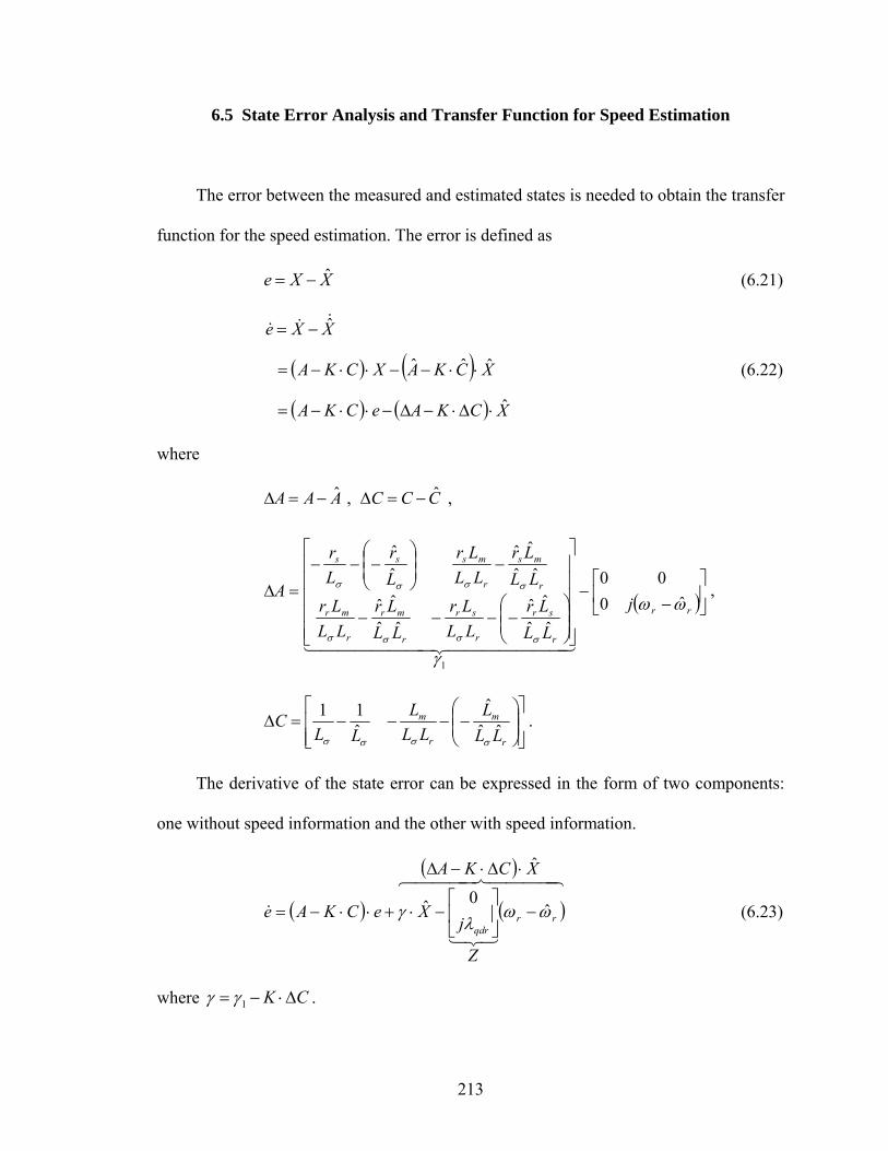
213

6.5 State Error Analysis and Transfer Function for Speed Estimation

The error between the measured and estimated states is needed to obtain the transfer

function for the speed estimation. The error is defined as

XXe ˆ−= (6.21)

( ) ( )( ) ( ) XCKAeCKA

XCKAXCKA

XXe

ˆ

ˆˆˆ

ˆ

⋅∆⋅−∆−⋅⋅−=

⋅⋅−−⋅⋅−=

−= &&&

(6.22)

where

CCCAAA ˆ,ˆ −=∆−=∆ ,

( )⎥⎦⎤

⎢⎣

⎡−

−

⎥⎥⎥⎥⎥

⎦

⎤

⎢⎢⎢⎢⎢

⎣

⎡

⎟⎟⎠

⎞⎜⎜⎝

⎛−−−−

−⎟⎟⎠

⎞⎜⎜⎝

⎛−−−

=∆rr

r

sr

r

sr

r

mr

r

mr

r

ms

r

msss

j

LLLr

LLLr

LLLr

LLLr

LLLr

LLLr

Lr

Lr

Aωω

γσσσσ

σσσσ

ˆ000

ˆˆˆˆ

ˆˆˆˆ

ˆˆˆˆ

ˆˆ

1

4444444 34444444 21

,

⎥⎥⎦

⎤

⎢⎢⎣

⎡⎟⎟⎠

⎞⎜⎜⎝

⎛−−−−=∆

r

m

r

m

LLL

LLL

LLC ˆˆ

ˆˆ11

σσσσ

.

The derivative of the state error can be expressed in the form of two components:

one without speed information and the other with speed information.

( ) ( )

( )4444 84444 76

321

&

XCKA

Z

jXeCKAe rr

qdr

ˆ

ˆ0ˆ

⋅∆⋅−∆

−⎥⎦

⎤⎢⎣

⎡−⋅+⋅⋅−= ωω

λγ (6.23)

where CK ∆⋅−= 1γγ .

214

The state error is solved as

[ ] ( )[ ]rrZXCKAIpe ωωγ ˆˆ1 −⋅−⋅⋅⋅+−⋅= − (6.24)

Then the output error can be expressed in terms of speed information and states.

( )

( ) [ ] ( )[ ] XCZXCKAIpCC

XCeCC

XCXC

IIYY

rr

qdsqds

⋅∆+−⋅−⋅⋅+−⋅⋅∆−=

⋅∆+⋅∆−=

⋅−⋅=

−=−

− ωωγ ˆˆ

ˆˆ

ˆˆ

1

(6.25)

The speed is estimated using (6.16) and (6.25).

( )[ ] ( ) ( )[ ] ( ) [ ] ( )[ ]

( ) ( ) [ ] ( )[ ] XCZXCKAIpCCkK

XCZXCKAIpCCkK

IIkIIkK

qdrrrqdr

qdrrrqdr

qdsqdsqdrqdsqdsqdrr

⋅∆⋅+−⋅−⋅⋅+−⋅⋅∆−⋅⋅−⋅+

⋅∆⋅+−⋅−⋅⋅+−⋅⋅∆−⋅⋅⋅=

−⋅⋅−+−⋅⋅⋅=

−

−

*1*

*1*

**

ˆˆˆˆRe1

ˆˆˆÎm

ˆˆRe1ˆÎmˆ

λωωγλ

λωωγλ

λλω

ω

ω

ω

(6.26)

To simplify the analysis, assume the parameters are constant, which means 0=∆C

and 0=γ . Then the speed estimation is simplified as

( )[ ] ( ) ( )[ ] [ ] ( )

( ) [ ] ( ) 44444444 344444444 21

T

rrqdr

rrqdr

qdsqdsqdrqdsqdsqdrr

ZCKAIpCkK

ZCKAIpCkK

IIkIIkK

ωωλ

ωωλ

λλω

ω

ω

ω

ˆˆRe1

ˆÎm

ˆˆRe1ˆÎmˆ

1*

1*

**

−⋅⋅+−⋅⋅⋅⋅−⋅−

−⋅⋅+−⋅⋅⋅⋅⋅−=

−⋅⋅−+−⋅⋅⋅−=

−

− (6.27)

Assuming [ ]CKAIp ⋅+−⋅ has the form

[ ] ⎥⎦

⎤⎢⎣

⎡=⋅+−⋅

2221

1211

PPPP

CKAIp

Then

215

( )21122211

2ˆˆ

PPPPjpj

LLL

Tr

mrrqdr −

−⋅⋅⋅−⋅−=

ωωωλσ

Define ⎥⎦

⎤⎢⎣

⎡++

=2221

1211

jKKjKK

K and 21211222111 jttPPPPT +=−= . Then

13122

22211212

211

2112

22

2112

22

2

1

tptp

LLLK

pLLLK

pLLLr

LK

LK

LLLrK

LLLrr

pLKp

Lr

pLLLrK

LLLrr

t

r

me

r

m

r

srrere

r

sr

r

srss

r

mre

r

mrs

++=

−−+−+

++++++−−−=

σσσσσ

σσσσσσ

ωωωωω

ω

,

2322

22

2122122

212111112

2

2

tpt

LLLrK

LLLK

LLLr

pLLLK

LLLrK

LK

LK

Lr

Lr

pLKppt

r

mr

r

me

r

ser

r

m

r

srrersesre

+=

−+−

−++−+−++−=

σσσσ

σσσσσσ

ωω

ωωωωωω

,

and

( ) ( ) ( )22

21

21212

ˆˆtt

tptjpttLL

LT ee

r

mrrqdr +

−++⋅⋅−⋅−=

ωωωωλ

σ

.

So

( ) ( ) ˆˆIm 22

21

212

tttpt

LLL

T e

r

mrrqdr +

−⋅⋅−⋅−=

ωωωλ

σ

( ) ( ) 22

21

122

ˆˆRett

tptLL

LT e

r

mrrqdr +

+⋅⋅−⋅−=

ωωωλ

σ

Define

( ) ( ) ˆˆ22

21

212

1 tttpt

LLL

pG e

r

mrrqdr +

−⋅⋅−⋅=

ωωωλ

σ

216

( ) ( ) 22

21

122

2 ˆˆtt

tptLL

LpG e

r

mrrqdr +

+⋅⋅−⋅=

ωωωλ

σ

Then

( ) ( ) ( )[ ] ( )rrr pGkpGkK ωωω ω ˆ1ˆ 21 −⋅⋅−+⋅⋅−= (6.28)

Define ( ) ( ) ( ) ( )pGkpGkpG 21 1 ⋅−+⋅= ,

then the transfer function between the

estimated speed and the actual speed is

( )( )pGKpGK

r

r

⋅+⋅

=ω

ω

ωω

1ˆ

(6.29)

where

( )01

22

33

401

22

33

bpbpbpbpapapapa

KpG G +++++++

⋅= (6.30)

( )( )

( ) ( )( )

( ) ,1

,1

,1

,

13230

122322131

22122

3

tktka

ttkttka

tkkta

ka

ee

ee

e

ωω

ωω

ω

−+−=

+−+−=

+−+=

=

,

,22

,2

,2

223

2130

232213121

22213

2122

123

ttb

ttttb

tttb

tb

+=

+=

++=

=

r

mqdrG LL

LK

σ

λ ⋅=2ˆ .

Assuming the controller is a general PI controller, the transfer function is

( )

( ) 012

23

34

45

012

23

34

4 1

ˆBpBpBpBpBp

ApApApApA

pGp

KK

pGp

KK

ip

ip

r

r

+++++++++

=⋅⎟⎟⎠

⎞⎜⎜⎝

⎛++

⋅⎟⎟⎠

⎞⎜⎜⎝

⎛+

=ω

ω

ωω

ωω

(6.31)

where,

217

( )( )( )

Gi

Gpi

Gpi

Gpi

Gp

KKaA

KKaKaA

KKaKaA

KKaKaA

KKaA

⋅=

⋅+=

⋅+=

⋅+=

⋅=

ω

ωω

ωω

ωω

ω

00

011

122

233

34

and

( )( )( )

Gi

Gpi

Gpi

Gpi

Gp

KKaB

KKaKabB

KKaKabB

KKaKabB

KKabB

⋅=

⋅++=

⋅++=

⋅++=

⋅+=

ω

ωω

ωω

ωω

ω

00

0101

1212

2323

334

. (6.32)

When 1=k , the analysis can be simplified as follows.

( )[ ]qdsqdsqdrr IIK ˆˆImˆ * −⋅⋅= λω ω (6.33)

The speed estimation is simplified assuming the parameters are constant, i.e.

0=∆C and 0=γ .

[ ] ( ) rrqdrr ZCKAIpCK ωωλω ω ˆˆImˆ 1* −⋅⋅+−⋅⋅⋅⋅−= − (6.34)

And

( ) ( )rrr pGK ωωω ω ˆˆ 1 −⋅⋅−=

where ( )01

22

33

401

22

3

1 bpbpbpbpapapap

KpG G +++++++

⋅= , and the transfer function between the

estimated speed and the actual speed is

( )( )pGKpGK

r

r

1

1

1ˆ

⋅+⋅

=ω

ω

ωω

(6.35)

Assuming the controller is a general PI controller, the transfer function is

( )

( )

( )( )pBpA

pGp

KK

pGp

KK

ip

ip

r

r =⋅⎟⎟⎠

⎞⎜⎜⎝

⎛++

⋅⎟⎟⎠

⎞⎜⎜⎝

⎛+

= 1

ˆ

1

1

ωω

ωω

ωω

(6.36)

where, ( ) 012

23

34

4 ApApApApApA ++++= ,

( ) 012

23

34

45 BpBpBpBpBppB +++++= ,

218

( )( )( )

Gi

Gpi

Gpi

Gpi

Gp

KKaA

KKaKaA

KKaKaA

KKaKA

KKA

⋅=

⋅+=

⋅+=

⋅+=

⋅=

ω

ωω

ωω

ωω

ω

00

011

122

23

4

and

( )( )( )

Gi

Gpi

Gpi

Gpi

Gp

KKaB

KKaKabB

KKaKabB

KKaKbB

KKbB

⋅=

⋅++=

⋅++=

⋅++=

⋅+=

ω

ωω

ωω

ωω

ω

00

0101

1212

223

34

. (6.37)

The above analysis is based on the assumption that the estimated speed is almost

identical to the actual speed. However, this is not always true. The transfer function

between the actual speed and the reference speed can be derived depending on the speed

controller. The dynamics of the speed controller is given by

( )rrr Kp ωωσω ωω ˆ*2 −⋅== (6.38)

Substituting for rω from (6.34), (6.37) results.

( )( ) ( )pAKpBp

pBK

r

r

ω

ω

ωω

+= 2* (6.39)

6.6 Observer Gain Selection

There are multiple choices for the observer gain (K11, K12, K21, and K22). Here, the

4th order Butterworth polynomial is applied. The idea of using the Butterworth

polynomial is to locate the poles of the transfer function evenly in the left half s-plane.

The locations of poles are shown in Figure 6.2. Since the complex form is used in the

formulation, only two solutions can be found. However the complex conjugates of these

two solutions yield the remaining two poles according to Figure 6.2 [6.9]. The four poles

are given as

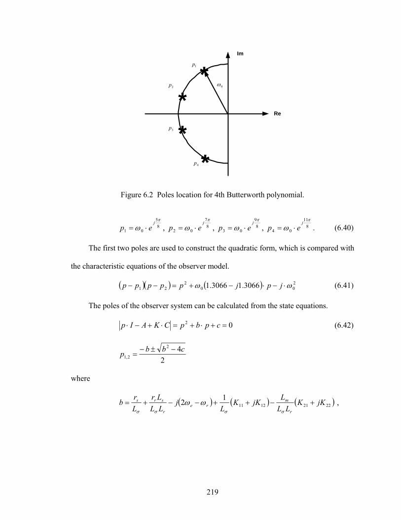
219

1p

2p

3p

4p

Im

Re

***

*

0ω

Figure 6.2 Poles location for 4th Butterworth polynomial.

85

01

π

ωj

ep ⋅= , 87

02

π

ωj

ep ⋅= , 89

03

π

ωj

ep ⋅= , 811

04

π

ωj

ep ⋅= . (6.40)

The first two poles are used to construct the quadratic form, which is compared with

the characteristic equations of the observer model.

( )( ) ( ) 200

221 3066.13066.1 ωω ⋅−⋅−+=−− jpjppppp (6.41)

The poles of the observer system can be calculated from the state equations.

02 =+⋅+=⋅+−⋅ cpbpCKAIp (6.42)

242

2,1cbbp −±−

=

where

( ) ( ) ( )2221121112 jKK

LLL

jKKL

jLLLr

Lr

br

mre

r

srs +−++−−+=σσσσ

ωω ,

220

( ) ( )

( ) ( ) ( )σσ

σσσσ

ωωωωωω

ωωω

LjKKj

LLjKKL

j

LLLr

jLr

jLL

jKKrLLrr

c

rer

meree

r

sre

sre

r

r

r

rs

12112221

1211

+

−−+

+−

−−−−+

+=

.

To ensure that the poles of the observer model are located according to the

Butterworth polynomial, the coefficients from (6.38) and (6.39) should be the same, i.e.

( ) 02212

02111

3066.12

3066.1

ωωω

ω

σσ

σσσσ

⋅=−+−

⋅=−++

r

mre

r

m

r

srs

LLKL

LK

LLKL

LK

LLLr

Lr

(6.43)

( ) ( )

( ) ( ) 20

112112

122211 0

ωωωωωωω

ωωωωωω

σσσσσ

σσσσ

=−

+−+−

+−

=−

+−−−+

LK

LLKL

LLLr

Lr

LLKr

LK

LLKL

LLKr

LLrr

re

r

me

r

sresre

r

r

re

r

meree

r

r

r

rs

(6.44)

Thus the four observer gains can be determined by choosing appropriate 0ω as

follows.

srr

reer

r

r

rr

r

rLLLr

LLr

Lr

K −⎥⎦

⎤⎢⎣

⎡−−⋅⋅⎟⎟

⎠

⎞⎜⎜⎝

⎛+⋅

+= 2

02

02

2

211 3066.11 ωωωωωωω

σσ

σ (6.45)

⎥⎦

⎤⎢⎣

⎡−+⋅⋅⎟⎟

⎠

⎞⎜⎜⎝

⎛−⋅

+= 2

02

02

2

212 3066.11 ωωωωωωω

σσσ

r

rreer

r

r

rr

r LLr

LLLr

Lr

K (6.46)

rm

s

m

r

rr

reer

r

r

rr

r

m

r

rLL

LLL

LLLr

LLr

Lr

LL

K

+⋅−

⎥⎦

⎤⎢⎣

⎡−−⋅⋅⎟⎟

⎠

⎞⎜⎜⎝

⎛+⋅

+=

0

20

20

22

221

3066.1

3066.1

ω

ωωωωωωω

σ

σσ

σ

(6.47)

221

( )m

rre

m

r

r

rreer

r

r

rr

r

m

r

LLL

LLL

LLr

LLLr

Lr

LL

K

σσ

σσσ

ωωω

ωωωωωωω

−−⋅+

⎥⎦

⎤⎢⎣

⎡−+⋅⋅⎟⎟

⎠

⎞⎜⎜⎝

⎛−⋅

+=

23066.1

3066.1

0

20

20

22

222

(6.48)

Theoretically a bigger value of 0ω will give better system response. In this case, the

value of 0ω is determined from the poles of the open-loop machine model. Those poles

can be calculated from the characteristic equation (6.49). The poles are given in [6.15].

When 0ω is taken as the sum of the imaginary parts of the poles, the expression for 0ω is

shown in (6.50).

( )

( ) ( ) 0

22

=⎥⎦

⎤⎢⎣

⎡−−−−−+

⋅⎥⎦

⎤⎢⎣

⎡−−++

r

sre

sreree

r

rs

rer

srs

LLLr

jLr

jLLrr

pjLLLr

Lr

p

σσσ

σσ

ωωωωωω

ωω

(6.49)

( )rer

srs jLLLr

Lr

pp ωωσσ

−+⎟⎟⎠

⎞⎜⎜⎝

⎛+−=+ 221

( ) ( )repp ωωω −⋅=+⋅= 221Im

21ˆ 2100 (6.50)

The relationship between the observer gains and 0ω is shown in Figure 6.3 for the

motoring mode and Figure 6.4 for the generating mode. The range of changing 0ω is

between 4/ˆ 00ω and 4/ˆ6 00ω while mL and rr change. It is seen that the parameters

change does not have much effect on K11 and K12. However, K21 and K22 are more likely

to be affected.

222

(a) (b)

(c) (d)


( rad/s 375 rad/s, 377 == re ωω in motoring mode). (a) 11K ; (b) 12K ; (c) 21K ; (d) 22K .

Solid line: =mL *mL , =rr


mL , =rr 1.25 *rr ; Dashdot line:

=mL 1.25 *mL , =rr 0.75 *

rr ; Dashed: =mL 0.75 *mL , =rr 1.25 *

rr ; Solid line (light):

=mL 0.75 *mL , =rr 0.75 *

rr .

223

(a) (b)

(c) (d)


( rad/s 379 rad/s, 377 == re ωω in generating mode). (a) 11K ; (b) 12K ; (c) 21K ; (d) 22K .

Solid line: =mL *mL , =rr


mL , =rr 1.25 *rr ; Dashdot line:

=mL 1.25 *mL , =rr 0.75 *

rr ; Dashed: =mL 0.75 *mL , =rr 1.25 *

rr ; Solid line (light):

=mL 0.75 *mL , =rr 0.75 *

rr .

224

Figures 6.5 and 6.6 show that the observer gains change with 0ω under different

operating conditions. The gains K11 , K12 , and K21 tend to decrease when the machine

enters the generating operation mode. But K22 tends to increase.

(a) (b)

(c) (d)


( *mm LL = , *

rr rr = , rad/s 390rad/s 360 rad/s, 377 ≤≤= re ωω ). (a) 11K ; (b) 12K ; (c)

21K ; (d) 22K .

225

(a) (b)

(c) (d)


( *mm LL = , *

rr rr = , rad/s 195rad/s 180 rad/s, 5.188 ≤≤= re ωω ). (a) 11K ; (b) 12K ; (c)

21K ; (d) 22K .

The observer gains are traditionally selected based on different considerations. In

[6.5 - 6.6, 6.17], the observer gains are determined by choosing the poles of the observer

model to be proportional to the poles of the machine model. In [6.16], the observer gains

226

are selected as 01211 == KK , srKK ⋅−== 25.02221 to ensure stability during

regenerating operation.

In [6.8], the observer gains are chosen as complex values in (6.51) to give enough

damping at high speeds.

⎥⎦

⎤⎢⎣

⎡⋅+−⋅+

=)ˆ(sign1

)ˆ(sign1

m

m

jj

Kωω

λ (6.51)

and ⎪⎩

⎪⎨

⎧

≥

<⋅=

λ

λλ

ωωλ

ωωωω

λλ

m

mm

ˆ if ,

ˆ if ,ˆ

'

'

(6.52)

where mω is the estimated rotor speed and λω is the base speed. 'λ and λω are selected

based on the linearized model of the observer. It also shows that by choosing the observer

gain as

⎥⎦

⎤⎢⎣

⎡−=

r

s

rr

K (6.53)

the error function in (6.15) for the speed estimation can be rewritten as (when k = 1)

( )[ ]( )[ ]qdsqdsqdr

qdsqdsqdr

ILL

II

σσ

λλ

λε

−⋅⋅−=

−⋅=

ˆÎm1

ˆÎm

*

*

(6.54)

The structure of the conventional MRAS for speed estimation is shown in Figure

6.1, in which the stator voltage equations are referred as the reference model and the rotor

voltage equations are referred as the adjustable model. The rotor flux linkages are

estimated in the stationary reference frame from the stator voltage equation (6.1) and

rotor voltage equation (6.2), respectively. The error function is defined as

( )[ ]qdsqdsqdr ILσλλε −⋅−= ˆÎm * (6.55)

227

The difference between (6.54) and (6.55) is the adaptation gain ( σL/1 ). Hence, the

conventional MRAS can be seen as a special case of the general speed-adaptive flux

observer defined in (6.12), (6.15) and (6.16). The operation when all the observer gains

are zero is discussed in [6.5 - 6.6, 6.8], which is an open-loop estimation. The proposed

method of determining the observer gains, however, could give good system response,

which is different from the original open-loop machine system.

6.7 D-decomposition Method

The denominator of the transfer function for the rotor speed in (6.36) is of 5th order.

It is therefore difficult to obtain an analytical solution to the eigenvalues. The D-

decomposition is then applied to determine the stability boundary (between the stable and

unstable regions) from the characteristic equation [6.10 - 6.12].

The idea of interpreting the stability conditions for linear systems in the parameter

plane has been generalized by Neimark in his D-decomposition method for consideration

of multiparameter problems. Consider a real polynomial, which is corresponding to the

characteristic equation of a transfer function,

( ) ∑=

=n

k

kk sasF

0 (6.56)

where the coefficients ka are continuous functions of r system parameters pi, that is

( )rkk pppaa ,,, 21 L= . ωσ js += is the complex variable in general. Now the r-

dimensional vector space, of which pi are coordinates, can be decomposed into sets

denoted by ( )mnmD −, , which correspond to the polynomial having m zeros with

228

negative and n-m zeros with positive real parts. Such a decomposition of the parameter

space into sets is called the D-decomposition.

The boundary of the sets ( )mnmD −, consists of those points for which the

polynomial ( )sF has finite zeros with vanishing real parts. The boundaries consist of

surfaces determined by

0 ,00 == naa (6.57)

and a surface determined by

( )

( )∑

∑

=

=

=

=

n

kkk

n

kkk

YaI

XaR

0

0

,0

,0

ω

ω (6.58)

where function ( )ω,0kX and ( )ω,0kY are given by the recurrence formulas

0

02

2

22

=+

=+

+

+

kk

kk

YY

XX

ω

ω (6.59)

with ω==== 1010 ,0,0,1 YYXX .

The surface 00 =a corresponds to a zero at the origin of the s plane and the surface

0=na corresponds to a zero at infinity of the s plane. The surface (6.58) corresponds to a

pair of pure imaginary zeros of the polynomial ( )sF .

Eliminating 2ω from (6.58), the following determinant is obtained.

0

00

0000

10

2223

1

1 ==∆

−−−−

−

−

n

nnnn

nn

n

aaa

aaaaaa

L

MMMMM

MMMMM

MMMMM

L

L

(6.60)

229

where 1−∆n is the next-to-the-last Hurwitz determinant n∆ of ( )sF . Thus the necessary

and sufficient condition for the polynomial ( )sF to have finite zeros with vanishing real

part is 0110 =∆ −naa .

The stability of a linear system with characteristic polynomial ( )sF is assured if a

point in the space is chosen from the set ( )0,nD . Points on the boundary of the set ( )0,nD

apparently satisfy the condition.

Although the D-decomposition is defined in a parameter space, it is convenient to

apply only to two-parameter problems. The common conditions for determing the

boundary of ( )0,nD provide two equations relating r parameters. In the case of two

parameters, the boundary of the stable and unstable regions can be determined from

(6.57) and (6.58). The conditions for (6.58) are equivalent to the ( )sF with substituting

ωjs = . By changing ω , certain curve (D-decomposition curve) can be drawn using the

two unkowns as the axis, which separate the stable and unstable regions. The stable

region is determined through a certain shading rule [6.10]. For the stability analysis, the

shading area is on the left half plane in the s-plane and the corresponding shading area in

the parameter plane is determined by calculating the determinant of Jacobian matrix. In

the case of the two parameters (α and β) problem, the Jacobian matrix is defined as

⎥⎥⎥⎥

⎦

⎤

⎢⎢⎢⎢

⎣

⎡

∂∂

∂∂

∂∂

∂∂

=

βα

βαII

RR

J (6.61)

where R and I are the real and imaginary parts of the characteristic equation when ωjs =

is substituted. If determinant of J ( det(J) ) is greater than 0, the shading area in the

parameter plane will be on the left hand side of the D-decomposition curve when ω is

230

increasing. If det(J) < 0, then the shading area in the parameter plane will be on the right

hand side of the D-decomposition curve when ω is increasing. The stable and unstable

regions can be determined through examing the real part of the roots of the characteristic

equation.

6.8 PI Control Parameters Selection

Choosing appropriate PI control parameters to regulate the error function of the

model reference adaptive mechanism is an important issue related to the stability of the

motor system. Some constraints have to be applied to the transfer function between the

estimated and actual speeds once it is known. First of all, all of the poles should be in the

left half s-plane, which complies that all poles have negative real parts. All of the zeros of

the transfer function also should have negative real parts such that the system is minimum

phase. The best way of checking the stability of a transfer function is using Routh table,

from which the conditions for the system to be stable can be found. However, those

coefficients in (6.37) are so complicated that it is difficult to find the explicit conditions.

The D-decomposition method is then applied to select the PI controller parameters, which

ensure that all the eigenvalues of the transfer function and zeros have negative real parts.

Two critical conditions need to be examined in this case. The first is that there is one

zero, and the other is that there is a purely imaginary pair for the eigenvalues. These

conditions are

0

0ωλ

λj±=

= (6.62)

Given in (6.36), the transfer function for the speed is

231

012

23

34

45

012

23

34

4ˆBpBpBpBpBp

ApApApApA

r

r

+++++++++

=ωω

To satisfy the first condition,

0or 00 230 ==⇒= tBλ (6.63)

which gives a certain constraint for choosing the observer gains under different operating

conditions. 23t is depending on the machine parameters and the observer gains. For this

case of study, it can be easily checked from computer simulation since the observer gains

are determined using the Butterworth polynomial method previously. Figure 6.7 shows

the relationship between 23t and oω , in which 23t is always less than zero. It means that

there is no pole at zero.

Figure 6.7 23t with respect to 0ω under different operating conditions ( *mm LL = ,

*rr rr = , rad/s 390rad/s 360 rad/s, 377 ≤≤= re ωω ).

232

To satisfy the second condition,

⇒±= 0ωλ j⎩⎨⎧

=+⋅−⋅=+⋅−

00

02

024

04

12

034

0

BBBBB

ωωωω (6.64)

Since all the B coefficients in (6.37) are the linear functions of pKω and iKω , the

relationship between pKω and iKω can be drawn when 0ω is changing. Figure 6.8 shows

the relationship under a particular operating condition when slip frequency is changing

from positive (motoring mode) to negative (generating mode). One basic condition for

choosing pKω and iKω is that both of them should be positive. By choosing two points

on the two sides of the curve, the eigenvalues and zeros can be calculated. From the

calculation, the region on the upper side is the stable region while the inner side is the

unstable region. This verifies that the PI controller parameters can be chosen arbitrary

large. However, noise will cause some problems when large values are used in the DSP

hardware implementation.

The above D-decomposition curve is corresponding to the condition when

∞<≠ ω0 . However, there is another constraint when 0=ω , which forms a straight line

(singular line) in the parameter plane [6.14]. The number of stable roots in each region

defined by this decomposition changes at two with crossing the curve and at one with

crossing a singular line. In the above case, the singular line is corresponding to the

condition when 0=iKω from (6.37). This condition is automatically satisfied when

0>iKω is chosen.

233

Figure 6.8 Relationship between Kwp and Kwi at different slip frequencies.

( rad/s 17rad/s 13- and rad/s 377 ≤≤= se ωω )

Only the active power is used as the error function in Figure 6.8. The drawback of

only using the active power as the error function is that the estimation at low speed range

is very bad. The performance of the observer system in the low speed region can be

improved by including the reactive power as part of the error function. The coefficient k

is defined as the partition factor between the active power and reactive power. The D-

decomposition curves change when k is changing between 0 and 1.

Figure 6.9 shows the D-decomposition curves for different k values. For different k

values, the stable region is always on the left side of the curves when 0ω is increasing

according to the shading rules. The similar trend can be observed that the stable region of

the controller parameters for the motoring operation is larger. Under the same operation

condition, the stable region corresponding to bigger k is also larger.

234

Figure 6.9 Relationship between Kwp and Kwi at different slip frequency. (a) k = 0.0; (b) k

= 0.2; (c) k = 0.4; (d) k = 0.5; (e) k = 0.8; (f) k = 1.0.

( rad/s 17rad/s 13- and rad/s 377 ≤≤= se ωω ).

(a)

(c) (d)

(e) (f)

(b)

235

The extreme cases for the parameter changes are now considered for the fixed k (k =

0.5). The changes in Lm and rr are considered within –50 percent and +50 percent. Then

the four extremes cases are ( * represent the nominal value )

1: ** 5.0 ,5.0 mmrr LLrr == ;

2: ** 5.1 ,5.0 mmrr LLrr == ;

3: ** 5.0 ,5.1 mmrr LLrr == ;

4: ** 5.1 ,5.1 mmrr LLrr == .

Figures 10 and 11 show the D-decomposition curves under the above extreme cases

in both motoring and generating modes. In the motoring operation mode, it is seen that

the stable region for the controller parameters is larger when Lm is fixed and rr has

positive error. The similar trend can also be observed when rr is fixed and Lm has positive

error. The stable region enlarges with the increasing rr and Lm . Also rr has more

influence on the stable region than Lm . However, in the generating operation mode, the

stable region for the controller parameters reduces when rr is fixed and Lm has positive

error although the stable region increases when Lm is fixed and rr has positive error. The

differences between the curves are much more significant in the generating mode than in

the motoring operation mode.

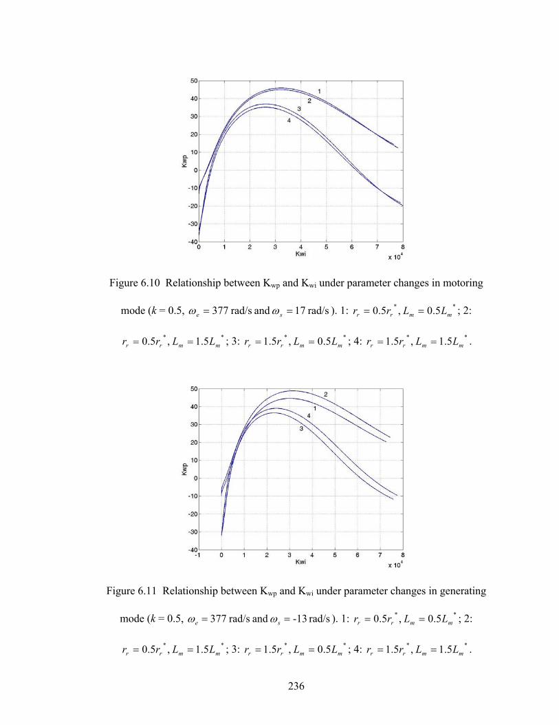
236

Figure 6.10 Relationship between Kwp and Kwi under parameter changes in motoring


** 5.1 ,5.0 mmrr LLrr == ; 3: ** 5.0 ,5.1 mmrr LLrr == ; 4: ** 5.1 ,5.1 mmrr LLrr == .

Figure 6.11 Relationship between Kwp and Kwi under parameter changes in generating



237

The above analysis shows the effects of the changing machine parameters on the

stable region of controller parameters. Those curves are useful for the selection of

controller parameters for the adaptive speed estimation. From the above analysis, the

speed estimation has to be considered in the design of the speed regulator. The transfer

function between the actual and reference speeds is also of a higher order. The D-

decomposition method can be applied to choose appropriate control parameters for the

speed regulation. The controller used to generate the second derivative of the rotor speed

is chosen as PD (proportion-differential) controller. The structure of the PD controller is

shown in Figure 6.12 and the transfer function between the actual and reference speeds is

derived below.

( )( )( )

( )( ) rrdrrrp

rrdrrrpr

ppBpAK

pBpAK

pKKp

ωωω

ωωωω

ωω

ωω

⋅⋅−⎟⎟⎠

⎞⎜⎜⎝

⎛⋅−=

⋅−−=

*

*2 ˆ

( )( ) ( ) ( )

( )( )pDpC

ppAKpAKppBpBK

rdrp

rp

r

r =⋅⋅+⋅+⋅

⋅=

ωω

ω

ωω

2* (6.65)

( ) ( ) ( )( ) ( )( ) rprdrp

rdrprdrp

rdrprd

KApKAKA

pKAKABpKAKAB

pKAKABpKABpBppD

ωωω

ωωωω

ωωω

001

2120

3231

4342

543

64

7

+⋅++

⋅+++⋅+++

⋅+++⋅++⋅+=

+

-

+

-

*rω

rω

rpKω ωσ

pK rdω

Figure 6.12 Structure of PD controller used for speed regulation.

238

Similar analysis has been done on the control design for the speed regulation. First,

the particular set of the controller parameters for the speed estimation is chosen such that

the system is stable for all of the operation conditions. This parameter set is then used to

generate the transfer function between the actual and reference speeds. From Figure 6.8,

the controller parameters for the speed estimation are chosen as 10000 ,50 == ip KK ωω .

The curves shown in Figure 13 corresponding to the generating operation mode are

located on the left side when 0ω is increasing. The stable region of the controller

parameters for the speed regulation increases with the increasing k since the stable region

is on the left side of the curves when 0ω is increasing according to the shading rules.

Figures 6.14 and 6.15 show the influence of parameter changes on the controller

parameters for the speed regulation. Similar trend can be observed as the D-

decomposition curves for the speed estimation. In the motoring operation mode, the

stable region for the controller parameters increases when Lm is fixed and rr has positive

error. The same trend is also observed when rr is fixed and Lm has positive error.

However, in the generating operation mode, the stable region for the controller

parameters reduces when rr is fixed and Lm has positive error although the stable region

increases when Lm is fixed and rr has positive error. The differences between the curves

are much more significant in the generating mode than in the motoring operation mode.

239

Figure 6.13 Relationship between Kwrd and Kwrp at different slip frequency. (a) k = 0.0;

(b) k = 0.2; (c) k = 0.4; (d) k = 0.5 (e) k = 0.8; (f) k = 1.0.

( rad/s 17rad/s 13- and rad/s 377 ≤≤= se ωω ).

(c) (d)

(e) (f)

(a) (b)

240

Figure 6.14 Relationship between Kwrd and Kwrp under parameter changes in motoring



Figure 6.15 Relationship between Kwrd and Kwrp under parameter changes in generating



241

6.9 Formulation of Control Scheme

The rotor flux oriented control is used for testing the proposed full-order flux

observer and adaptive speed estimation. The stator and rotor voltage equations are used

again to formulate the whole control scheme. The objectives of the control are to regulate

the rotor speed and operate the induction motor under the specified rotor flux linkages

( drλ is constant and 0=qrλ ). The stator and rotor voltage equations are rewritten as

drr

mrqr

r

mrdseqsqsqsqs L

LLLr

ILVrIpIL λωλωσ σσ −+−==+ 2 (6.66)

qrr

mrdr

r

mrqsedsdsdsds L

LLLr

ILVrIpIL λωλωσ σσ +++==+ 2 (6.67)

( ) drreqsr

mrqrqr

r

rqr I

LLr

Lrp λωωσλλ −−==+ (6.68)

( ) qrredsr

mrdrdr

r

rdr I

LLr

Lrp λωωσλλ −+==+ (6.69)

( )J

PTIIKp Ldsqrqsdrer 2−−= λλω (6.70)

In the control scheme, the PI controller parameters for the adaptive speed estimation

are chosen based on the analysis in section 6.8. For all the other controllers, the transfer

functions are found first and then the parameters are determined using the Butterworth

polynomial by choosing appropriate 0ω . Two controllers are used to maintain qrdr λλ , as

the desired values. The corresponding transfer functions can be derived as follows.

242

∗dsI

∗rω

CBA III ,,

AB

C

qrλ

*qsV

Inverter*dsV

rω

+

+

esω eω

qsσ

DSQS II ,

∗drλ

+-

drλ

rKω

-+

rω

∗qsI

dsqs II ,

-

∗qrλ + qrσ

drK

ωσ Eq.6.70

+-

Eq.6.66qsK

qsI

dsσdrσ Eq.6.69

+-

Eq.6.67dsK

dsI

Eq.6.68qrK

( )0T( )θT

Motor

( )θ1−T&

Sine-PWM

312111 ,, SSS

1/s

ObserverModel

ωKdsqs

drqr

II ˆ,ˆ

ˆ,ˆ λλ ** , dsqs VVEq.6.15

Figure 6.16 Rotor flux oriented control including full-order flux observer and adaptive

speed estimation.

From (6.69),

( )

r

rdr

dr

dr

dr

drdrdrdrr

rdr

Lr

pK

K

KLr

p

++=

−⋅=+

*

*

λλ

λλλλ

(6.71)

From (6.68),

( )

r

rqr

qr

qr

qr

qrqrqrqrr

rqr

Lr

pK

K

KLr

p

++=

−⋅=+

*

*

λλ

λλλλ

(6.72)

The other two controllers are used to maintain qsds II , at the desired values. The

corresponding transfer functions can be derived from (6.66) and (6.67) as follows.

243

( )

rpLKK

II

IIKrIpIL

qs

qs

qs

qs

qsqsqsqsqs

++=

−⋅=+

σ

σ

*

*

(6.73)

( )

rpLKK

II

IIKrIpIL

ds

ds

ds

ds

dsdsdsdsds

++=

−⋅=+

σ

σ

*

*

(6.74)

The transfer function between the actual and reference speeds is given in (6.65).

In the simulation, general PI controllers are used and the parameters are calculated

by assuming particular 0ω from the transfer functions when compared with the second

order Butterworth polynomial. The machine parameters are

sr = 1.9812 Ω, rr = 1.85 Ω,

sL = 0.2077 H, rL = 0.2077 H, mL = 0.1986 H,

eω = 377 rad/s, rω = 375 rad/s, qdrλ = 0.4.

When 0ω is chosen 300 rad/s,

The PI controller parameters for drλ ( drK ) are 46517 and 125 == ip KK .

The PI controller parameters for qrλ ( qrK ) are 90000 and 415 == ip KK .

The PI controller parameters for qsI ( qsK ) are 1602 and 9.3 == ip KK .

The PI controller parameters for dsI ( dsK ) are 1602 and 9.3 == ip KK .

The PD controller parameters for rω ( rKω ) are 500 and 50000 == dp KK .

The PI controller parameters for rω ( ωK ) are 10000 and 50 == ip KK .

The estimator gains are chosen corresponding to the analysis as

6887.011 =K , 3792.212 =K , 1175.021 =K , 0419.022 =K .

244


The actual induction motor model and the observer model are included in the

computer simulation. The two sets of stator currents used for the speed estimation are

coming from these two models respectively. The same q- and d-axis voltages are applied

to these two models. The flux linkages are estimated from the voltage equations and then

the currents are calculated from these flux linkages.

Simulations have been done based on the proposed control scheme, which includes

the rotor flux oriented control, full-order flux observer, and adaptive speed estimation.

The rotor speed is ramped up to the rated value (377 rad/s) during the starting period. The

speed reference reaches the steady state at t = 2 seconds. A full load (4Nm) is applied to

the motor at t = 3 seconds and then the load is removed at t = 4 seconds. A negative load

(-4Nm) is applied to test the operation of the motor in the regenerating mode.

The reference, actual and estimated speeds are shown in Figure 6.17(a). It is seen

that the feedback speed, which is the estimated speed, tracks the reference speed very

well. The actual speed is almost the same as the estimated one, although small difference

can be seen among these three speeds from Figure 6.18. The torque developed in the

induction motor is shown in Figure 6.17(b), which is corresponding to the load torque

except for some ripples due to the switching of the converter.

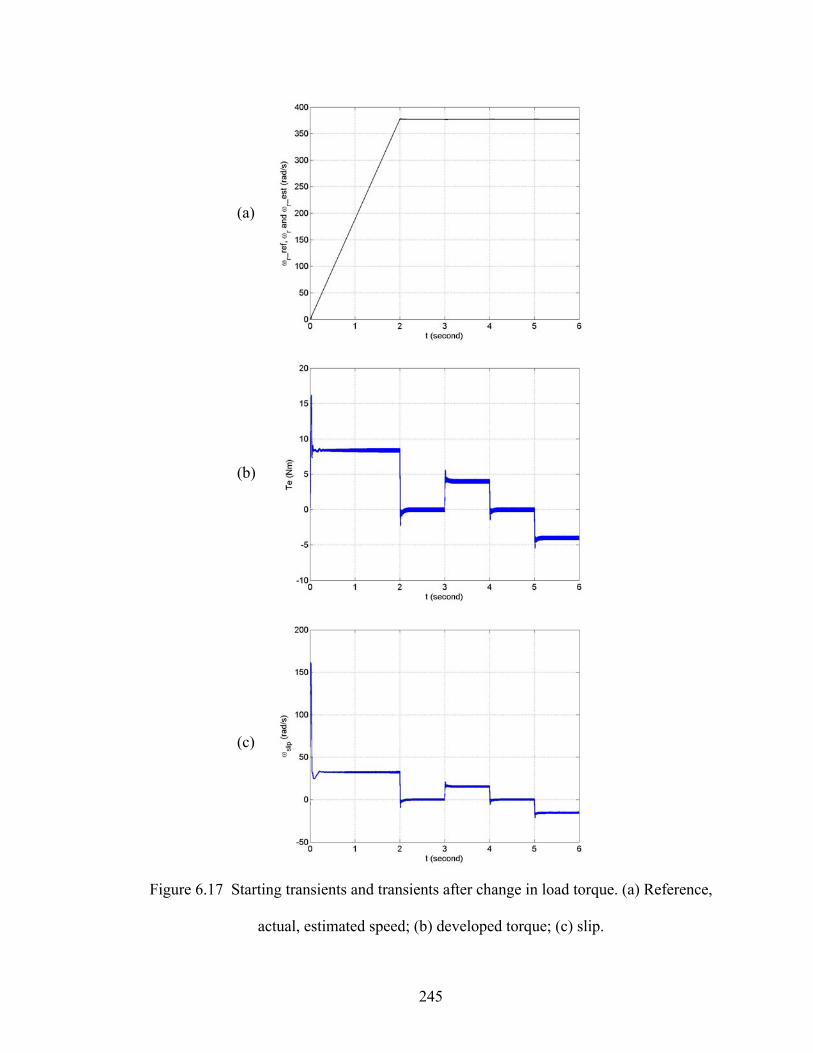
245

Figure 6.17 Starting transients and transients after change in load torque. (a) Reference,

actual, estimated speed; (b) developed torque; (c) slip.

(a) (b) (c)

246

The differences between the actual and estimated q- and d-axis currents are shown

in Figure 6.19. The differences are not zero during transience while they are zero at the

steady state, which means that the estimated speed converges to the actual speed

according to the adaptive speed mechanism. Figure 6.20 shows the regulations for the

four controllers regulating the q- and d-axis rotor flux linkages and q- and d-axis stator

currents. It is shown that both rotor flux linkages are regulated to the reference values

except for small oscillations during the load change. The stator currents are also regulated

although there are ripples in the estimated current, which are due to the switching of the

converter. Figure 6.21 shows the actual and estimated rotor flux linkages in stationary

reference frame. Figure 6.22 shows the actual and estimated stator and rotor flux

linkages, which are almost identical.

The speed changes after the motor speed gets to the steady state are made to check

the capability of proposed design under no-load condition. The estimated speed tracks the

reference very well and it is almost identical to the actual speed seen in Figure 6.23(a).

The speed changes have the similar effects as load changes from Figure 6.23(b).

247

(a) (b)

(c) (d)

Figure 6.18 Starting transients and transients after change in load torque: reference,

actual and estimated speeds (a) during starting; (b) after starting; (c) at the steady state;

(d) zoomed around the reference speed.

248

Figure 6.19 Starting transients and transients after change in load torque. (a) Difference

between actual and estimated q-axis currents; (b) difference between actual and estimated

d-axis currents.

(a) (b)

249

(a) (b)

(c) (d)

Figure 6.20 Starting transients and transients after change in load torque. (a) Regulation

of drλ ; (b) regulation of qrλ ; (c) regulation of Iqs; (d) regulation of Ids.

250

Figure 6.21 No-load flux linkages at steady state. (a) Actual q- and d-axis rotor flux

linkages; (b) estimated q- and d-axis rotor flux linkages.

(a) (b)

251

(a) (b)

(c) (d)

Figure 6.22 Starting transients and transients after change in load torque. (a) Actual and

estimated qsλ ; (b) actual and estimated dsλ ; (c) actual and estimated qrλ ; (d) actual and

estimated drλ .

252

Figure 6.23 Response to the change in speed. (a) Reference, actual, estimated speed; (b)

developed torque.

(a) (b)

253

6.11 Conclusion

This chapter analyzes a full-order flux observer system. The model is used to

estimate the rotor speed of an induction motor through the adaptive mechanism. The

observer gains are chosen using 4th order Butterworth polynomial. The transfer function

between the estimated and actual speeds is found based on the error analysis, which is

used to determine the PI controller parameters for the speed estimation ensuring the

operation in the stable region. The rotor flux oriented control including the observer and

adaptive speed estimation is designed to examine the proposed methods. The controller

parameters are determined from the corresponding transfer functions. The whole system

is simulated in both motoring and regenerating modes. It is shown that all the controllers

are working properly and the rotor speed is regulated very well under different load

conditions, which validate the proposed method of designing full-order flux observer and

speed estimation.

254

CHAPTER 7

GENERALIZED OVER-MODULATION METHODOLOGY FOR CURRENT

REGULATED THREE-PHASE VOLTAGE SOURCE CONVERTERS

7.1 Introduction

Operation of three-phase voltage source converters in the over-modulation regions

could improve steady-state capabilities and dynamic system performance in the motor

drive and utility applications. Both carrier-based PWM and space vector PWM operating

in the linear modulation region have been discussed in Chapter 2, in which the

equivalence between these two modulation schemes is found. However, their

characteristics in the over-modulation region are quite different although some

similarities are still there. In the case of carrier-based PWM, the modulation index has to

be increased in the over-modulation region in order to generate the desired fundamental

voltage since the modulation signal is clipped when it is out of the range between -1 and

1. For the space vector PWM, the sum of the calculated times spent on the two active

states will be greater than 1, which is not realizable. The way of generating higher

fundamental voltage is to adjust the trajectory of the voltage vector such that the voltage

vector stays in the region in which the voltage is realizable for a longer time.

Correspondingly the times spent on the active states will be adjusted to generate more

fundamental voltage.

In this chapter, a more parsimonious equivalency/relationship between the two

modulation schemes for converter operation in both linear and over-modulation regions

255

will be established using a partitioning parameter. A space vector algorithm is then

proposed based the on-time for the top switching devices, which gives higher

fundamental voltages than the scaling scheme. Both PWM schemes are applied in the

current regulation using the linear controller and the fundamental current as the feedback

through eliminating the load harmonic current. The mitigation control schemes based on

load harmonic current estimation and use of anti-windup controllers are proposed to

achieve high dynamic over-modulation performance. The confirmatory experimental

results are given to demonstrate the effectiveness of the current control concept for all

possible operating regions.

7.2 Linear PWM Modulation Schemes

In the direct digital PWM method, the complex plane stationary reference frame qd

output voltage vector of the three-phase voltage source inverter is used to calculate the

turn-on times of the inverter switching devices required to synthesize a reference three-

phase balanced voltage set. In general, the three-phase balanced voltages expressed in the

stationary reference frame; situated in the appropriate sector in Figure 7.1(b) are

approximated by the time-average over a sampling period (converter switching period,

Ts) of the two adjacent active qd voltage inverter vectors and the two zero states U0 and

U7. The switching turn-on times of the two active and two null states are utilized to

determine the duty cycle information to program the active switch gate signals [7.3].

When the inverter is operating in the linear modulation region, the sum of the turn-on

times of the two active switching modes is less than the switching period, in which case

256

the remaining time is occupied by using the two null vectors, U0 and U7. If the

normalized times for which the set of four voltage vectors Vqda, Vqdb, Vqd0, Vqd7 are called

into play are ta , tb, t0, t7, respectively, then the q and d components of the reference

voltage Vqd* are approximated as

Vqd* = V*

q + jV*d = Vqdata + Vqdbtb + Vqd0t0 + Vqd7t7,

tc = t0 + t7 = 1 - ta - tb , ∇ = [ Vdb Vqa - VqbVda] (7.1)

ta = [ Vq* Vdb -Vd

*Vqb]/∇, tb = [ Vd*Vqa - Vq

*Vda]/∇

Table 7.1 gives the total times the upper three top devices of the converter are

turned on. The sum of these normalized times (ta + tb) is usually less than one for

operation in the linear modulation region. Then the two null states can be appropriated

for the remaining time, tc, in which the normalized times for the null states are defined as

to = βtc and t7 = (1 - β)tc , respectively. For the classical space vector (SVPWM) , β = 0.5

for which all the switches are switching all the time during the switching period. PWM

schemes are known to reduce the effective converter switching frequency and switching

loss when some of the devices are clamped either to the positive or/and negative rails

during a switching cycle. This device clamping is realized in the space vector PWM

when the total device turn-on time is equal to the switching period. Table 7.1 reveals that

when t7 = tc (β = 0), the normalized on-time of one of the three top devices is unity for all

the sectors – a top device is always clamped to the positive rail. Similarly, when tc = t0 (t7

= 0, β = 1.0), a top device will always be clamped to the negative rail. When the partition

parameter is defined as in (7.2) in which a modulation phase angle δ is variable, a

generalized space vector PWM (GSVPWM) results.

β = 0.5·[1 - Sgn (Cos (3ωt + δ))] (7.2)

257

The relationship between the SVPWM and GDPWM is now set forth. Figure 7.1(a)

shows a schematic diagram of a three-phase voltage source inverter in which the

switching devices in the same leg are turned on complimentarily. The phase voltage

equations for star-connected, balanced three-phase loads expressed in terms of the

existence functions (Sip) of devices (Tip) and input dc voltage Vd are given as

0.5 Vd (2Sap - 1) = 0.5 Vd Map = Vap + Vpn

0.5 Vd (2Sbp - 1) = 0.5 Vd Mbp = Vbp + Vpn (7.3)

0.5 Vd (2Scp - 1) = 0.5 Vd Mcp = Vcp + Vpn

Sip = 0.5 (1 + Mip) , i = a, b, c

In equations in (7.1), Vap, Vbp, Vcp are the phase voltages of the load while the

voltage of the load neutral to inverter reference is Vpn. The modulation signals for the

three top devices are Map , Mbp , Mcp . The equations for the generalized modulating

signals of the top devices are expressed as [7.2]

Table 7.1 The turn-on normalized times for three top devices

Sector 1 2 3 4 5 6

τap ta+tb+t7 ta+t7 t7 T7 tb+t7 ta+tb+t7

τbp tb+t7 ta+tb+t7 ta+tb+t7 ta+t7 t7 t7

τcp t7 t7 tb+t7 ta+tb+t7 ta+tb+t7 ta+t7

258

Load

pnb

a

c

2Vd

2Vd

apT bpT cpT

cnTbnTanT

(a)

Im

Re

U2 (110)U3 (010)

U0

(000) U1 (100)

U5 (001)

U4 (011)

U6 (101)

U7

(111) ⎥⎦

⎤⎢⎣

⎡ −6

,0,3

2 dd VV

⎥⎦

⎤⎢⎣

⎡−

633ddd V,V,V

⎥⎦⎤

⎢⎣⎡ −−−

6,

3,

3ddd VVV

⎥⎦⎤

⎢⎣⎡−

60

32 dd V,,V

⎥⎦

⎤⎢⎣

⎡−−

6,

3,

3ddd VVV

⎥⎦

⎤⎢⎣

⎡6

,3

,3

ddd VVV

at

bt *qdV

(b)

Figure 7.1 (a) Schematic diagram of a voltage source inverter, (b) qdo voltages for the

switching states.

Mip = 2Vip/Vd + 2Vpn/Vd, i = a,b,c (7.4)

Vpn = 0.5Vd (1-2β) − βVmin - (1-β)Vmax (7.5)

In (7.5) Vmax and Vmin are the instantaneous maximum and minimum magnitudes of

the three reference balanced phase voltages, respectively. The carrier-based modulation

signals which yield the same voltage waveforms as the classical space vector are obtained

259

when β in (7.5) is set equal to 0.5. However, other definitions of β in (7.2) with a variable

modulation phase angle δ gives an infinite number of possibilities leading to the

generalized discontinuous carrier-based triangle intersection PWM modulation method.

Hence, the generalized space vector(GSVPWM) and the generalized discontinuous

carrier-based triangle intersection(GDPWM) PWM, using the same value of β in (7.2) in

the generation of the turn-on times or modulation signals yield fundamental output

voltages with the same characteristics and hence are equivalent especially when operating

in the linear modulation region.

7.3 Modulation in the Overmodulation Regions

Given the reference voltage as V*qd, the modulation magnitude index of a PWM

inverter is defined as

2

*

d

qd

V

VM

⋅=

π

Figure 7.2 shows the qd voltage trajectories of the inverter operating in the linear

and over-modulation regions. When the inverter is operating in the linear region with the

classical space vector modulation (β = 0.5), it generates sinusoidal three-phase voltages

which follow the qd trajectory represented by the dark circle. The magnitude of the

reference voltage lies within the inner circle of the hexagon and the magnitude

modulation index ranges between zero and 0.907 (0.0 ≤ M ≤ 0.907). The inverter goes

into the over-modulation region when part of the qd voltage vector is located outside the

inner circle. The over-modulation region is further divided into two regions according to

260

the characteristics of the trajectory. In Figure 7.2(b) where (0.907 ≤ M ≤ 0.95),

corresponding to Region I over-modulation region, the inverter follows the trajectory of

the dark line which generates the reference fundamental qd voltage represented by the

inner dotted line. When the dark line reaches the vertices of the hexagon, the trajectory

changes to that in Figure 7.2(c) representing the over-modulation region II (0.95 ≤ M ≤

1.0). In this case, the voltage vector stays at the vertices for enough time to generate the

desired fundamental voltage [7.5].

In the space vector modulation scheme operating in the over-modulation region, the

sum of the calculated times for the two adjacent active voltage states is greater than the

switching period (ta + tb > 1) when the reference voltage vector is outside the hexagon. To

satisfy the time constraint, times (ta , tb) are traditionally scaled down with respect to the

switching period as shown in (7.6) to yield a new timing (t*a , t*

b)

ba

bb

ba

aa tt

tt

ttt

t+

=+

= ** , (7.6)

Under this scheme one of the top devices is clamped to the positive rail and another

top device is clamped to the negative rail while the third one is switching under PWM.

Another slightly different scheme based on Table I is proposed here which generates a

higher fundamental voltage. For a device with a total normalized turn-on time greater

than unity (ta + tb + t7 > 1), the turn-on time is forced to be 1 (example: τap =1 in sector 1).

Also, since the normalized device turn-on times must be positive and less than unity, t7

and ta + t7 or tb + t7 (depending on the sector) must satisfy these constraints: t7 ≥ 0, ta + t7

≤ 1 or tb + t7 ≤ 1. Hence, if the new times are ta*, tb

*, t7*, the algorithm becomes

261

q

d

α

*Mq

d

q

d

Figure 7.2 Voltage trajectories in the inverter. (a) Linear region; (b) over-modulation

region I; (c) over-modulation region II.

(a) (b) (c)

262

0 ≤ ta + tb + t7 ≤ 1 ⇒ ta* + tb

* + t7* = 1

0 ≤ ta + t7 , tb + t7 ≤ 1 ⇒ t7* ≤ 1 - ta , 1 - tb (7.7)

0 ≤ t7 ≤ 1

In this formulation, t7* can be chosen as t7

* = ε (1 - ta), ε (1 - tb) while 0 ≤ ε ≤ 1.

Hence, in general, only one top device is clamped to the positive rail and the other two

top devices are switching in the over-modulation region. Although an infinite possibilities

exist, ε = 0 gives the highest fundamental voltage reference when two top devices are

clamped (one to the positive rail and the other to the negative rail ) as shown in Table 7.2.

Note that in this case the time the switching top device is turned on is greater than the

corresponding time for the traditional scaling solution.

For the inverter operating in the over-modulation regions, the generalized

discontinuous carrier-based triangle intersection modulation scheme does not suffer the

timing constraint of the generalized space vector; rather when the modulation signal is

higher than the carrier signal, the device stays continually turned on – naturally limiting

the fundamental component of the synthesized voltage.

Table 7.2 The turn-on normalized times for three top devices in the over-modulation

region

Sector 1 2 3 4 5 6

τap 1 ta 0 0 tb 1

τbp tb 1 1 ta 0 0

τcp 0 0 tb 1 1 ta

263

7.4 Open-loop Voltage Generation

The classical space vector or generalized discontinuous triangle intersection PWM

in which β = 0.5 can be used to generate the fundamental voltage in the linear region (M

≤ 0.907). However, another space vector method and a generalized discontinuous triangle

intersection PWM with α value of unity or zero have to be applied when the fundamental

generated voltage is to be increased in the over-modulation region. The original voltage

reference trajectory to be used as input to the modulator in the space vector PWM scheme

needs to be changed in order to obtain the desired fundamental voltage since the

reference voltage vector cannot be generated when it is out of the hexagon. The

modification of the reference voltage vector introduces voltage harmonic components

which are also reflected in the actual load voltage vector. In the over-modulation region I,

the trajectory of reference voltage vector is changed from the inner circle to the dark line

in Figure 7.2(b). When the voltage reference is within the hexagon, the classical space

vector modulation is used and the suggested algorithm in Table II is implemented when

the voltage trajectory lies on the hexagon. Analyzing q-axis voltage of the reference

voltage trajectory gives the fundamental and harmonic components. As shown in Figure

7.2(b), particular crossover angle α or M* (new modulation magnitude index, new

voltage reference) can be found for a given reference voltage [7.5].

For a given voltage reference, the phase voltage waveform is divided into three

segments for each sector. The voltage equations in each segment are expressed as (in

sector 1)

264

⎟⎠⎞

⎜⎝⎛ −

⋅=

απθ

32sin3

cosdcq

VV , for αθ <≤0 (7.8)

⎟⎠⎞

⎜⎝⎛ −

⋅−=

απθ

32sin3

sin32 dc

dcqV

VV , for απθα −<≤3

(7.9)

⎟⎠⎞

⎜⎝⎛ −

⋅=

απθ

32sin3

cosdcq

VV , for

33πθαπ

<≤− (7.10)

where tωθ = and ω is the angular velocity of the fundamental voltage reference vector.

Expanding the above equations in all of six sectors in a Fourier series and taking the

fundamental component of it, the relationship between the crossover angle and

modulation index can be found in Figure 7.3. The red one represents the relationship for

the traditional scaling space vector modulation methods.

Similarly, the voltage trajectory in the over-modulation region II is modified from

the inner circle to the dark line as shown in Figure 7.2(c). The major difference in this

region is that the voltage vector stays at the vertices of the hexagon for some time (or

corresponding holding angle αh) and then moves along the edges. The voltage equations

in each segment are expressed as (in sector 1)

dcq VV32

= , for hαθ <≤0 (7.11)

⎟⎠⎞

⎜⎝⎛ −

⋅−=

'

'

32sin3

sin32

θπθdc

dcqV

VV , for hh απθα −<≤3

(7.12)

dcq VV31

= , for 33πθαπ

<≤− h (7.13)

265

Figure 7.3 Relationship between crossover angle and modulation index in region I.

where

66

' π

απαθ

θ ⋅−

−=

h

h (7.14)

The relationship between the holding angle and modulation index can be found in

Figure 7.4.

Figure 7.5 displays the comparison between the proposed turn-on time allocation

and the classical scaling method after combining the above two figures. In over-

modulation region I, for the same crossover angle, the new proposal yields higher

modulation magnitude index (fundamental voltage) than that from the classical method.

The same trend is seen in over-modulation region II until the two methods eventually

yield the same fundamental voltage magnitude (modulation magnitude index) when the

holding angle gets close to 0.524 radian (the six-step operation).

266

Figure 7.4 Relationship between holding angle and modulation index in region II.

Figure 7.6 also shows the plot of the new modulation magnitude index command

(M*) required to generate a desired voltage for the GDPWM scheme calculated from

results in [7.3]. Similar to the approach of using space vector, the mapping curve showing

the relationship between the reference and actual modulation signals needs to create first

in the overmodulation region. It's also calculated through Fourier series method. The

equations used for the three PWM methods are listed as following.

SVPWM, space vector PWM

When 3

* π≤M ,

2

****

321

23

32arcsin3

21

⎟⎟⎠

⎞⎜⎜⎝

⎛−+⎟⎟

⎠

⎞⎜⎜⎝

⎛⋅⋅+−=

MMMMM ππ

π;

When 3

* π>M

2

***

61

21

6arcsin3

⎟⎠⎞

⎜⎝⎛−+⎟

⎠⎞

⎜⎝⎛⋅⋅=

MMMM ππ

π.

DPWM1, which is corresponding to the discontinuous PWM for δ = 0°.

267

Figure 7.5 Relationship between the crossover / holding angle and modulation

magnitude index.

2

*

**

**

321

23

32arcsin31

342131

⎟⎟⎠

⎞⎜⎜⎝

⎛−+

⎟⎟⎠

⎞⎜⎜⎝

⎛⋅⋅+⋅+⎟⎟

⎠

⎞⎜⎜⎝

⎛−+−=

M

MM

MMM

π

ππ

ππ

DPWM2, which is corresponding to the discontinuous PWM for δ = -30°.

When 3

* π≤M ,

21

21

*1

***

1

*

2

32sin2

343

3cos

21

62cos

43

23

6sin

23

4

32arcsin

3

baM

Mb

MMMa

M i

+=

⎟⎟⎠

⎞⎜⎜⎝

⎛⎟⎠⎞

⎜⎝⎛ −−−×+⎟

⎠⎞

⎜⎝⎛ +−=

⎟⎠⎞

⎜⎝⎛ +−+⎟

⎠⎞

⎜⎝⎛ −−=

⎟⎟⎠

⎞⎜⎜⎝

⎛+−=

πψψππ

πψ

πψππ

ψπψ

ππψ

;

268

When 3

* π>M ,

21

21

*1

**1

*

2

23322sin

21

43

23

2cos

322cos

43

43

83

21

2sin

32arcsin

32

baM

Mb

MMa

M

+=

⎟⎟⎠

⎞⎜⎜⎝

⎛−+⎟

⎠⎞

⎜⎝⎛ −−×+−=

⎟⎠⎞

⎜⎝⎛ −−⎟⎟

⎠

⎞⎜⎜⎝

⎛−−+=

⎟⎟⎠

⎞⎜⎜⎝

⎛−=

αππαπ

α

παππ

απ

α

ππα

;

It is seen that in the overmodulation region, the actual modulation index M is

calculated for the open-loop voltage generation when the desired modulation index is M*.

For the three cases displayed, the highest voltage gain (lowest M*) is obtained when δ =

0º.

Figure 7.6 Mapping of the reference and actual modulation magnitude index for

operation in the over-modulation region.

269

7.5 Current Regulation

Current regulation is generally required in most high performance motor drive

applications in which the q and d axis stator currents are generally regulated to ensure

torque or speed control. Standard proportional plus integral (PI) type controller

implemented in the synchronous reference frame is usually adequate for most practical

applications. However, when the modulator is required to operate in the over-modulation

and six-step regions, the synchronous reference frame PI controller has been found to be

inadequate due to its inability to regulate or reject the harmonic currents flowing in the

load which are impressed by the added harmonic voltages. Although the harmonic

current component of the load current can be filtered using a high pass filter, they lead to

a slower system response requiring the current bandwidth to be reduced if the feasibility

of control loop instability is to be minimized. An innovative solution for this problem

which is applicable when the inverter is under space vector modulation is given in [7.6].

Instead of filtering the load current, the harmonic current is estimated and removed from

the measured current, the balance of which is regulated using the classical synchronous

reference frame PI controller. The actual reference voltage for the space vector

calculation needed for the synthesis of the required fundamental load voltage vector is

obtained from the off–line gain mapping shown in Figure 7.5. Through experimental

results, it was shown that this scheme works well even up to the six-step operation.

In another development for an inverter using the discontinuous carrier-based

triangle intersection PWM and operating in the over-modulation regions, because the

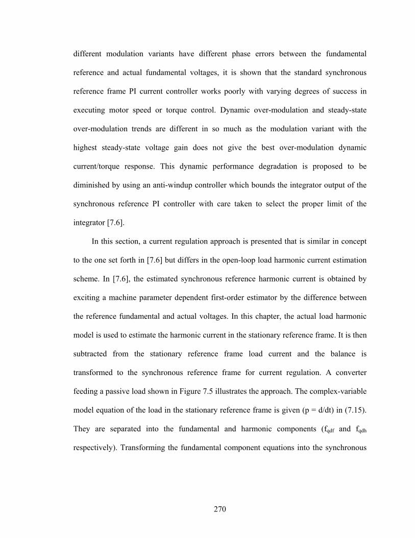
270

different modulation variants have different phase errors between the fundamental

reference and actual fundamental voltages, it is shown that the standard synchronous

reference frame PI current controller works poorly with varying degrees of success in

executing motor speed or torque control. Dynamic over-modulation and steady-state

over-modulation trends are different in so much as the modulation variant with the

highest steady-state voltage gain does not give the best over-modulation dynamic

current/torque response. This dynamic performance degradation is proposed to be

diminished by using an anti-windup controller which bounds the integrator output of the

synchronous reference PI controller with care taken to select the proper limit of the

integrator [7.6].

In this section, a current regulation approach is presented that is similar in concept

to the one set forth in [7.6] but differs in the open-loop load harmonic current estimation

scheme. In [7.6], the estimated synchronous reference harmonic current is obtained by

exciting a machine parameter dependent first-order estimator by the difference between

the reference fundamental and actual voltages. In this chapter, the actual load harmonic

model is used to estimate the harmonic current in the stationary reference frame. It is then

subtracted from the stationary reference frame load current and the balance is

transformed to the synchronous reference frame for current regulation. A converter

feeding a passive load shown in Figure 7.5 illustrates the approach. The complex-variable

model equation of the load in the stationary reference frame is given (p = d/dt) in (7.15).

They are separated into the fundamental and harmonic components (fqdf and fqdh

respectively). Transforming the fundamental component equations into the synchronous

271

reference frame rotating at ωe, the model to be used for controller design for the

fundamental load current component results in (7.17).

Vqd = rs Iqd + Ls p Iqd + Eqd (7.15)

Vqd = Vqdf + Vqdh , Iqd = Iqdf + Iqdh (7.16a)

Vqdf = rs Iqdf + Ls p Iqdf + Eqd (7.16b)

Vqdh = rs Iqdh + Ls p Iqdh (7.16c)

Vqde = rs Iqde + Ls p Iqde - j ωe Iqde + Eqde (7.17)

In Figure 7.7, the harmonic load current in the stationary reference frame is

estimated based on (7.16c). When the inverter is space vector modulated, the harmonic

voltage is obtained from the difference between the actual space vector voltage trajectory

shown in Figure 7.2 and the command fundamental voltage all expressed in the stationary

reference frame. This current is subtracted from the measured current expressed in the

stationary reference frame, the balance of which is the fundamental load current which

expressed in the synchronous reference frame is used for the current regulation using the

synchronous reference frame PI controllers. If the modulation method is the generalized

discontinuous carrier-based triangle intersection PWM modulation, the harmonic voltage

is obtained from the difference between the load voltage estimated using the converter

switching functions and the reference fundamental voltage expressed in the stationary

reference frame. Furthermore, in Figure 7.7, there is a gain-mapping block (G, which are

Figures 7.5,6 for the space vector and carrier-based triangle intersection modulations,

respectively) which maps the reference fundamental voltage (modulation magnitude

index) to the actual modulation magnitude index (load fundamental voltage). In the

carrier-based scheme the angle of the fundamental reference voltage is preserved in the

272

fundamental voltage mapping scheme. From (7.10) and Figure 7.7, the controller

structure with a controller (Kqd = PI or IP) is determined as follows.

Vqde* = σqde - j ωe Iqde + Eqde (7.18)

σqde = rs Iqde + Ls p Iqde = Kqd (Iqde* - Iqde)

The transfer function of the current control (where Kqd = Kp + Ki/p) is

( ) ips2

s

ip*qde

qde

KpKrpLKpK

II

+++

+= (7.19)

The controller parameters are appropriately selected to meet desired dynamic

response specifications and system stability.

While the current control scheme (7.18) ensures current regulation when a

converter operates in the over-modulation region, it may not give a good speed/torque

control of a motor drive since torque pulsation producing harmonic currents are still

present in the motor. A viable way to remedy this limitation is to use a modulation

scheme which produces the least harmonic load voltage. Furthermore, a natural reference

current regulator to eliminate or reduce the most important harmonic current component

is added to the motor control algorithm, the output of which is added to the reference

voltage generated by the synchronous reference frame PI controller to modulate the

inverter to minimize the generated load harmonic voltage.

273

*qdeI

ba II ,

A

B

C

qdeV

Inverter

qdeσ+

-

qdeI

PWM

qdI

qdV

+

-

seLjω

+

+

qdfV

qdK

qdeE

- Synchronous->

Stationary

( )θT

Stationary->

Synchronous

( )θ1−T

Stationary

( )0T

Load qdfqd VV −ˆ

qdfIqdeI

Load

GFig. 3Fig. 4

Estimator

aEsL

bEsLsr

cEsLsr

sr+ -

+ -

+ -

qdhI

Figure 7.7 Diagram of current regulation in all modulation regions.

The current regulation in the overmodulation region is simulated through changing

the reference currents. The reference currents are changed corresponding to Figure 7.8, in

which the two currents are selected such that the operation is in the linear modulation

region first. And then these two currents are ramped up to generate enough reference

voltages and make the operation in the overmodulation region. It is seen that the two

currents in the synchronous reference frame are regulated very well using the proposed

method. The phase currents for the fundamental and harmonic components are shown in

Figure 7.9. The harmonic component appears in the overmodulation region. But it has

been eliminated effectively such that this component does not affect the regulation of

fundamental q- and d-axis currents.

274

Figure 7.8 Simulation of current regulation for q- and d-axis currents. (a) Q-axis

reference current; (b) q-axis actual current; (c) the output from the current controller for

q-axis current; (d) d-axis reference current; (e) d-axis actual current; (f) the output from

the current controller for d-axis current.

(a) (b) (c) (d) (e) (f)

275

Figure 7.9 Simulation of current regulation. (a) Phase A fundamental current during the

transient; (b) phase A harmonic current during the transient; (c) phase A fundamental

current at steady state in the overmodulation region; (d) phase A harmonic current at

steady state in the overmodulation region.

(a)

(b) (c) (d)

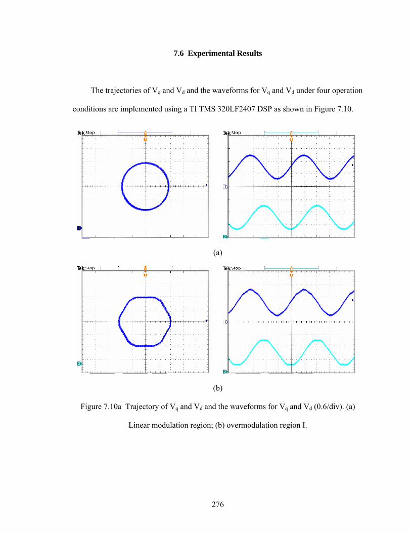
276


The trajectories of Vq and Vd and the waveforms for Vq and Vd under four operation

conditions are implemented using a TI TMS 320LF2407 DSP as shown in Figure 7.10.

(a)

(b)

Figure 7.10a Trajectory of Vq and Vd and the waveforms for Vq and Vd (0.6/div). (a)

Linear modulation region; (b) overmodulation region I.

277

(a)

(b)

Figure 7.10b Trajectory of Vq and Vd and the waveforms for Vq and Vd (0.6/div). (a)

Overmodulation region II; (b) six step operation.

The proposed current control technique and the modulation schemes have been

implemented using the TMS 320LF2407 DSP. The experiments have been done by step

changing the q and d-axis reference currents while the magnitudes of the current ensure

transitions from one operation region to another. The three-phase wye-connected passive

load has a per-phase resistance of 1.93 Ohms and a per-phase inductance of 56.65 mH.

278

The switching frequency of the converter is 10 kHz, load current frequency is 60 Hz and

the DC input voltage is 150 V. The implementation procedure is as follows.

1. Determine the relationship between the crossover angle α / holding angle hα

and the magnitude of reference voltage using either linearization method or

lookup table, which is corresponding to simulation results.

2. Check the region of current reference voltage and find the corresponding angle

if it is in the overmodulation regions.

Linear modulation: use continuous / discontinuous method;

Overmodulation I: use curve for the crossover angle;

Overmodulation II: use curve for the holding angle.

3. In the overmodulation region I, for example in sector I,

When αθ <<0 , use linear modulation;

When αθα −°<< 60 , use the proposed method for the overmodulation: use

( )απ −⋅ 3/2sin3dcV

as the magnitude of reference voltage, θ as the

actual angle;

When °<<−° 6060 θα , use linear modulation again.

4. In the overmodulation region II, for example in sector I,

When hαθ <<0 , hold the switching pattern at vertex 1;

When hh αθα −°<< 60 , calculate the actual angle to be used,

66/π

απαθ

θ ⋅−

−=′

h

h , use dcV32 as the magnitude of reference voltage, θ ′

279

as the actual angle and then use the proposed method for the

overmodulation;

When °<<−° 6060 θα h , hold the switching pattern at vertex 2.

In the implementation of the control scheme, the actual phase voltages are required

in order to find the harmonic currents. There are two ways of doing this: either measuring

the voltages using voltage sensors or using switching functions to reconstruct the phase

voltages. The formulations are shown in (7.20).

( )

( )

( )cpbpaps

dccs

cpbpaps

dcbs

cpbpaps

dcas

TV

V

TV

V

TV

V

τττ

τττ

τττ

23

23

23

+−−⋅=

−+−⋅=

−−⋅=

(7.20)

where τap, τbp and τcp are the on-durations for the three top devices calculated from

symmetric sine-PWM and Ts is the switching period.

The control system using the space vector modulation scheme (with the mapping

gain block) is implemented and Figure 7.11 shows the q and d-axis currents, line-line

voltage and phase current when the reference currents are varied to make the inverter

transition from one region to another. It can be seen that the axes currents are regulated

appropriately for the three regional transitions. Figure 7.12 gives phase ‘a’ currents in the

three operational regions. The synthesized fundamental load currents obtained by

removing the harmonic load are also displayed. In the same figure, the voltage

trajectories during transitions are shown.

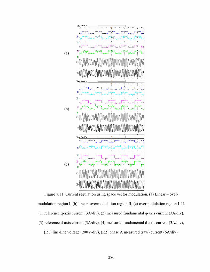
280

Figure 7.11 Current regulation using space vector modulation. (a) Linear – over-

modulation region I; (b) linear–overmodulation region II; (c) overmodulation region I–II.

(1) reference q-axis current (3A/div), (2) measured fundamental q-axis current (3A/div),

(3) reference d-axis current (3A/div), (4) measured fundamental d-axis current (3A/div),

(R1) line-line voltage (200V/div), (R2) phase A measured (raw) current (6A/div).

(a) (b) (c)

281

Figure 7.13 shows corresponding current regulation results when the inverter is

modulated with the discontinuous carrier-based triangle intersection modulation (with the

mapping gain accounted for) and δ = 0°. The current regulation is very good. Figure 7.14

shows the estimated harmonic currents (with converter operating in the linear and over-

modulation regions) which when subtracted from the load currents make load current

regulation possible. The fundamental currents feedback for current control is very clean

even when the converter is operating in over-modulation region II.

Finally, one questions whether the mapping block G is really needed in the current

control system to achieve good current regulation using discontinuous PWM. It would

appear, based on limited computer simulation studies that the current regulation is

achieved without accounting for mapping gain when the converter operates in the over-

modulation region. The important consideration therefore to good current regulation

using the decoupling control scheme shown in Figure 7.7 is not so much on the type of

modulation scheme, but on the ability to remove the load harmonic current from the

current control loop.

However, for speed and torque control, modulation schemes giving minimum

harmonic voltage components with the current regulation in Figure 7.5 should be very

effective. Figure 7.15 displays the current regulation using the discontinuous carrier-

based triangle intersection modulation with δ = 0° without including the non-linear

mapping gain. The current regulator works well for all transitions from linear to the over-

modulation regions of operation. Experimental results confirmed by simulation results do

not show any increase of converter actuating reference voltages when compared to the

case when the mapping gain is included in the control scheme. Apparently, the

282

decoupling terms in the expression of the reference voltage (7.18) ensures the appropriate

matching of the reference and the fundamental component of the actual voltage –

minimizing both the magnitude and phase errors.

Figure 7.12a Voltage (Vq –Vd) trajectories using space vector modulation (25V/div). (a)

Linear to over-modulation region I transition; (b) linear to over-modulation region II

transition.

(a) (b)

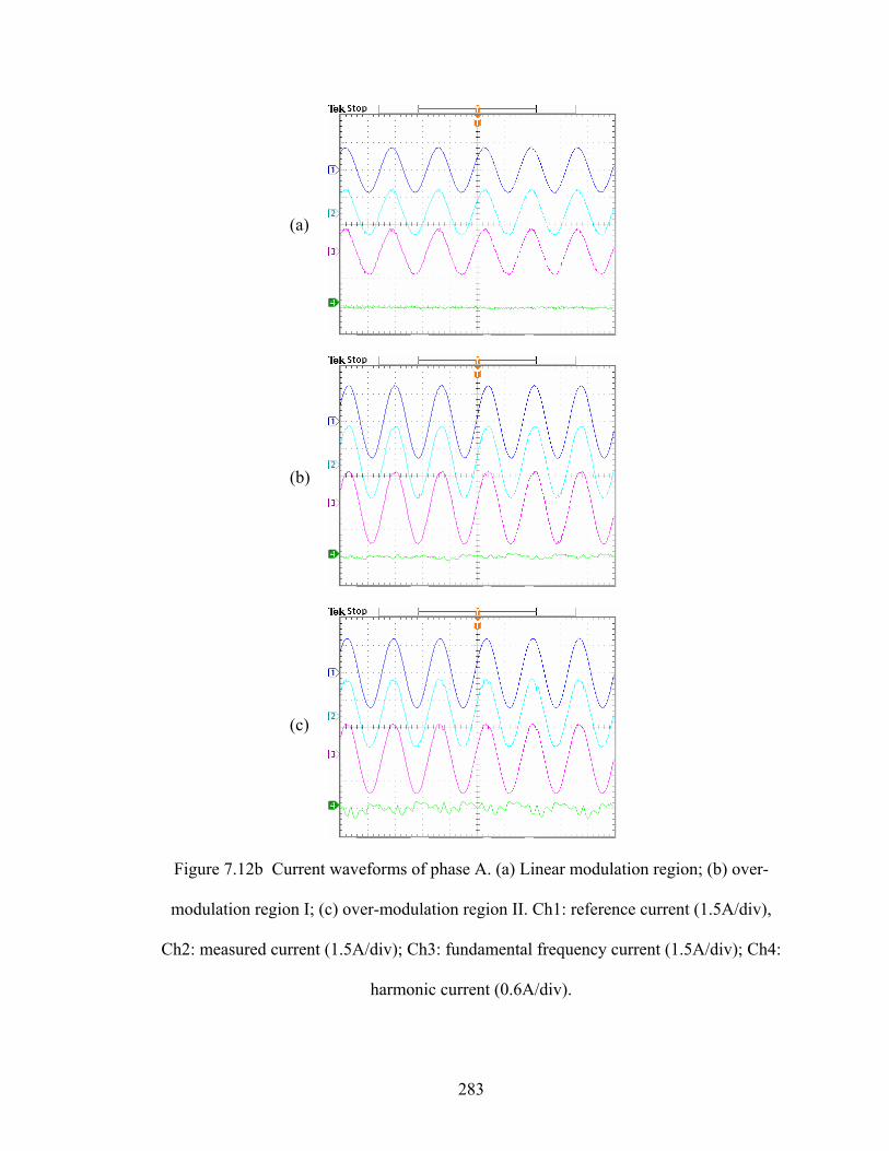
283

Figure 7.12b Current waveforms of phase A. (a) Linear modulation region; (b) over-

modulation region I; (c) over-modulation region II. Ch1: reference current (1.5A/div),

Ch2: measured current (1.5A/div); Ch3: fundamental frequency current (1.5A/div); Ch4:

harmonic current (0.6A/div).

(a) (b) (c)

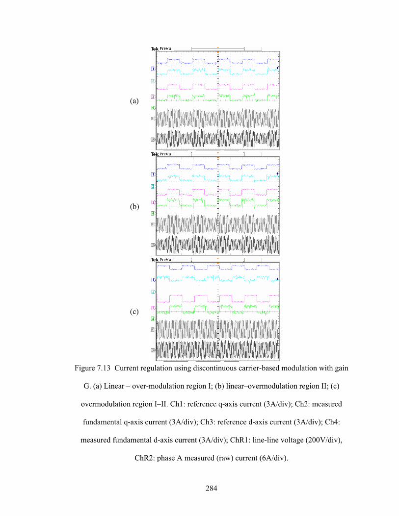
284

Figure 7.13 Current regulation using discontinuous carrier-based modulation with gain

G. (a) Linear – over-modulation region I; (b) linear–overmodulation region II; (c)



measured fundamental d-axis current (3A/div); ChR1: line-line voltage (200V/div),

ChR2: phase A measured (raw) current (6A/div).

(a) (b) (c)

285

Figure 7.14 Current waveforms of phase A using discontinuous carrier-based modulation

with gain G. (a) Linear modulation region; (b) over-modulation region II; (c) over-

modulation region II. Ch1: reference current (1.5A/div); Ch2: measured current

(1.5A/div); Ch3: fundamental frequency current (1.5A/div); Ch4: harmonic current

(0.6A/div).

(a) (b) (c)

286

Figure 7.15 Current regulation using discontinuous carrier-based modulation without

gain G. (a) Linear – over-modulation region I; (b) linear–overmodulation region II; (c)



measured fundamental d-axis current (3A/div); ChR1: line-line voltage (200V/div);

ChR2: phase A measured (raw) current (6A/div).

(a) (b) (c)

287

7.7 Conclusion

This chapter developed and unified the generalized space vector (GSVPWM) and

generalized discontinuous carrier-based (GDPWM) PWM methods in the linear and over-

modulation regions. A time-varying partition factor β (which is time-varying in general

and ranging between zero and unity) provides an equivalency link between the two

schemes. An algorithm that provides a higher fundamental voltage than the time-scaling

procedure traditionally used for space vector PWM modulator for voltage synthesis in the

over-modulation region is also proposed.

Then the load current regulation of a current regulated voltage source inverter is

explored accounting for the nonlinear converter gain introduced when operating in the

over-modulation regions. A current decoupling and linearizing control scheme with the

harmonic current estimation process is used to ensure good current regulation even when

the converter operates in the over-modulation region for both the generalized space

vector and the generalized discontinuous carrier based triangle intersection modulation

schemes. Some experimental results have been provided to confirm the validity of the

control and estimation schemes for the two modulation methods. It would appear that

with a good load harmonic estimation algorithm and a decoupling linearizing control

structure, any modulator scheme with a high open loop voltage gain characteristics will

provide a high performance closed loop current characteristics with or without

accounting for the converter gain nonlinearity. The modulation phase angle δ which gives

different GDPWM and GSVPWM schemes can indeed be regulated on-line to ensure the

288

nulling of the phase angle between the reference and actual voltage vectors – a phase

angle difference which has been proven to negatively influence the over-modulation

response of the controlled drive systems.

289

CHAPTER 8

CONCLUSIONS AND FUTURE WORK

This chapter summarizes the contributions made by this dissertation. The

contributions in different areas are described in separate paragraphs. The previous work

done in these areas has been detailed in Chapter 1 to establish some background on the

work carried out in this dissertation. The scope for future work is discussed and some

suggestions are made based on the work developed.

8.1 Conclusions

The PWM modulation techniques for the three-phase voltage source inverter are

presented including both carrier-based PWM and space vector PWM. The equivalence is

set up between these two methods for the normal operation. The concept of space vector

is extended to the multi-phase systems in the example of five and six phases. The space

vector diagram is drawn using the generalized transformation and then used to synthesize

the reference voltages. For the multi-phase system, the reference voltage other than the

fundamental one can be generated, which can be third harmonic component when the

single machine is running or other sequence component that can be used to drive the

other motor in series. The calculation of zero sequence voltage expressions is done by

choosing the appropriate active and null states and then these expressions are generalized

and added to the reference voltage to generate the modulation signals. The switching

290

signals are generated using carrier-based PWM through the comparison between these

modulation signals and the high frequency carrier signals. This method is easy to

implement compared with the direct space vector approach and can be used for any

multi-phase system.

The induction machine model in the arbitrary reference frame and the general

transformations are presented explicitly, which are used for the control analysis of

induction machines. The procedure of determining the machine parameters is presented

and used to determine the parameters of the experimental induction machine. Then the

rotor flux oriented control of the induction machine is illustrated and the cascaded speed

control scheme is designed. The controller parameters are designed using Butterworth

polynomial and the implementation procedures are presented in detail, which are useful

for the design and implementation of any other control system. The proposed scheme has

been verified through simulations and experiments.

The natural variables are defined for the induction machine and then used to

formulate the speed control, which are all calculated in stationary reference frame and no

reference frame transformation is necessary. The efficiency of the induction machine is

improved through the minimum electrical loss strategy formulated using the same

variables. The optimum rotor flux is resulted from the strategy and used as the reference

one in the speed control. Also the rotor speed estimation using both rotor voltage

equations is proposed and the simulation shows much better estimation result. The

experiments are conducted to verify the proposed formulation and the sensorless method.

The closed-loop speed estimation using the full-order flux observer is explored and

the design process is illustrated for the speed control. The consideration of including the

291

reactive power in the error function for the speed estimation improves the performance in

the low speed range. The observer gains are determined using the 4th order Butterworth

polynomial and the control parameters for the speed estimation are selected using the D-

decomposition method to ensure the system stability. It is shown that the same set of

parameters can be chosen from the proposed method to make the system stable under

both motoring and regenerating modes. The characteristics of the full-order flux observer

and the effectiveness of proposed method of selecting parameters have been shown in the

simulation results.

The modulation characteristics for the carrier-based PWM and space vector PWM

are found in over-modulation region. A new over-modulation scheme is proposed using

the concept of space vector, which has a higher voltage gain compared with the

traditional scaling method. The application for the current regulation is generalized for

both modulation methods and the idea of eliminating the harmonic current in stationary

reference frame is proposed in order to use the linear controller structure and generate

higher fundamental voltages in the over-modulation region. Both PWM methods are

implemented for the current regulation on the R-L load and the comparison is made on

the analysis of advantages and disadvantages.

8.2 Future Work

There are several possible areas for future research based on the sensorless control

of induction machines and associated PWM modulation schemes presented in this

dissertation. Although the modulation technique for three-phase voltage source

292

converters has been extended to the multi-phase system including five and six phases, the

effect of selecting the active states and zero sequence voltages on the real multi-phase

machine are not verified through experiments yet. It is expected that the electric torque

performance of the induction machine can be possibly improved by using different states

and zero sequence voltages.

The proposed sensorless approach using the full-order flux observers can also be

used for the rotor speed sensorless control for the permanent magnet machine. The other

application of this full-order flux observer system is for the multi-phase machines

combined with the modulation scheme proposed in this dissertation. The procedures of

selecting the observer gain and controller parameters are applicable for motor control

system designs ensuring system stability.

The control using natural variables can be extended to the control of the multi-

phase machines, which could also be used for loss minimization. The over-modulation

technique for three-phase system and the idea of eliminating harmonic currents are

helpful to enhance the robustness of multi-phase machine systems under both normal and

faulty operating conditions.

293

REFERENCES

294

[2.1] A. Schonung and H Stemmler, “Static frequency changers with subharmonic control in conjunction with reversible speed ac drives,” Brown Boveri Rev., vol. 1, no. 51, nos. 8/9, pp. 555-557, Sept. 1964.

[2.2] G. Pfaff, A. Weschta, and A Wick, “ Design and experimental results of a

brushless ac servo drive,” IEEE Transactions on Industry Applications, IA-20, pp. 814-821, 1984.

[2.3] J A Houldsworth and D. A. Grant,“ The use of harmonic distortion to increase the

output voltage of the three phase PWM,” IEEE Transactions on Industry Applications, vol. 24 , pp. 142-150, 1988.

[2.4] A. Hava, R. J. Kerkman and T. A. Lipo, “A High Performance Generalized

Discontinuous PWM Algorthim,” IEEE Transactions on Industry Applications, vol. 34, no. 5, pp. 1059-1071, September/October 1998.

[2.5] L. Xu and W. N. Fu, “Evaluation of third harmonic component effects in five-

phase synchronous reluctance motor drive using time-stepping finite element method,” IEEE Transactions on Industry Applications, vol. 38, no. 3, pp. 638 – 644, May/June 2002.

[2.6] R. O. Lyra and T. A. Lipo, “Torque density improvement in a six-phase induction

motor with third harmonic current injection,” IEEE Transactions on Industry Applications, vol. 38, no. 5, pp. 1351 – 1360, Sep./Oct. 2002.

[2.7] E. Levi, M. Jones and S. N. Vukosavic, “ Even-phase multi-motor vector

controlled drive with single inverter supply and series connection of stator windings,” IEE Proceeding - Electric Power and Applications, vol. 150, no. 5, pp. 580 – 590, September 2003.

[2.8] E. Levi, M. Jones, N. Vukosavic and H. A. Toliyat, “ A novel concept of a

multiphase, multimotor vector controlled drive system supplied from a single voltage source inverter,” IEEE Transactions on Power Electronics, vol. 19, no. 2, pp. 320 – 335, March 2004.

[2.9] E. Levi, S. N. Vukosavic and M. Jones, “Vector control schemes for series-

connected six-phase two-motor drive systems, IEE Proceedings – Electric Power and Applications, vol. 152, no. 2, pp. 226 – 238, April 2005.

[2.10] O. Ojo, “The generalized discontinuous PWM scheme for three-phase voltage

source inverters,” IEEE Transactions on Industrial Electronics, vol. 51, no. 6, pp. 1280 – 1289, December 2004.

[2.11] E. A. Klingshirn, “High power order induction motors, - Part I – Description and

theoretical consideration,” IEEE Transactions on Power Systems and Apparatus, vol. 102, no. 1, pp. 46 – 53, January 1983.

295

[2.12] M. A. Abbas, R. Christen and T. M. Jahns, “ Six-phase voltage source inverter

driven induction motor,” IEEE Transactions on Industry Applications, vol. 20, no. 5, pp. 1251 – 1259, September/October 1984.

[2.13] H. A. Toliyat, S. Waikar and T. A. Lipo, “Analysis and simulation of five phase

synchronous machines including third harmonic of airgap MMF,” IEEE Transactions on Industry Applications, vol. 34, no. 2, pp. 332 – 339, March/April 1998.

[2.14] L. Parsa and H. A. Toliyat, “Five-phase permanent magnet motor drives,” IEEE

Transactions on Industry Applications, vol. 41, no. 1, pp. 30 – 37, Jan./Feb. 2005. [2.15] L. Xu, “ Rotor structure selections of nonsine five-phase synchronous reluctance

machines for improved torque capability,” IEEE Transactions on Industry Applications, vol. 36, no. 4, pp. 1111 – 1117, July/August 2000.

[2.16] H. M. Ryu, J. W. Kim and S. K. Sul, “ Synchronous frame current control of

multi-phase synchronous motor. Part I – Modeling and current control based on multiple d-q spaces concept under balanced condition,” Conference Record of the Annual Meeting of the IEEE Industry Applications Society, pp. 63 – 70, October 2004.

[2.17] Y. Zhao and T. A. Lipo, “Space vector PWM control of dual three-phase

induction machine using vector space decomposition,” IEEE Transactions on Industry Applications, vol. 31, no. 5, pp. 1177 – 1184, September/October 1995.

[2.18] D. Hadiouche, L. Baghli and A. Rezzoug, “Space vector PWM techniques for

dual three-phase ac machines: Analysis, performance evaluation and DSP implementation,” Conference Record of the annual meeting of the IEEE Industry Applications Society, pp. 648-655, October 2003.

[2.19] C. B. Jacobina, R. S. Miranda, M. B. Correa, A. M. Lima and N. Rocha, “ Five

phase converter dual-winding ac drive systems,” Conference Record of the IEEE International Electric Machines and Drives Conference, pp. 1345 – 1349, May 2005.

[2.20] J. W. Kelly, E. G. Strangas and J. M. Miller, “Multi-phase space vector pulse

width modulation,” IEEE Transactions on Energy Conversion, vol. 18, no. 2, pp. 259 – 264, June 2003.

[2.21] H. M. Ryu, J. H. Kim and S. K. Sul, “Analysis of multi-phase space vector pulse-

width modulation based on multiple d-q space concepts,” To appear in the IEEE Transactions on Power Electronics.

296

[2.22] G. J. Retter, Matrix and Space-Phasor Theory of Electrical Machines, Akademiai Kiado, Budapest, Hungary, 1987.

[2.23] P. J. Davis, Circulant Matrices, Chelsea Publishing Company, 1979. [2.24] A. Hava, R. J. Kerkman and T. A. Lipo, “ A high performance generalized

discontinuous PWM algorithm,” IEEE Transactions on Industry Applications, vol. 34, no. 5, pp. 1059 – 1071, September/October 1998.

[4.1] Myoung-Ho Shin, Dong-Seok Hyun, Soon-Bong Cho and Song-Yul Choe, “An

improved stator flux estimation for speed sensorless stator flux orientation control of induction motors”, IEEE Transaction on Power Electronics, vol. 15, no. 2, pp. 312-317, 2000.

[4.2] X. Xu and D. W. Novontny, “Implementation of direct stator flux orientation

control on a versatile DSP based system”, IEEE Transaction on Industry Applications, vol. 27, no. 4, pp. 694-700, 1991.

[4.3] L. Harnefors, “Design and analysis of general rotor-flux oriented vector control

systems,” IEEE Transactions on Industrial Electronics, vol. 48, pp. 383-389, April 2001.

[4.4] B. K. Bose and N. R. Patel, “A programmable cascaded low-pass filter-based flux

synthesis for a stator flux-oriented vector-controlled induction motor drive”, IEEE Transaction on Industrial Electronics, vol. 44, no. 1, pp. 140-143, 1997.

[4.5] I. Kioskeridis and N. Margaris, “Loss minimization in scalar-controlled induction

motor drives with search controllers,” IEEE Transactions on Power Electronics, vol. 11, no. 2, pp. 213-220, March 1996.

[4.6] M. P. Kazmierkowski, R. Krishnan and F. Blaabjerg, Control in Power

Electronics : Selected Problems, Academic Press, 2002. [4.7] Zhenyu Yu, “Space-vector PWM with TMS320C24x/F24x using hardware and

software determined switching patterns”, Application Report, Texas Instruments, 1999.

[4.8] Olorunfemi, Ojo, “Field orientation control of a doubly-fed synchronous

reluctance machine”, Research Report 98-01, 1998. [4.9] Ahmet M. Hava, Russel J. Kerkman, and Thomas A. Lipo, “Simple analytical and

graphical methods for carrier-based PWM-VSI drives”, IEEE Transactions on Power Electronics, vol. 14, no. 1, pp. 49-61, 1999.

297

[4.10] Riccardo Marino, Sergei Peresada and Paolo Valigi, “Adaptive input-output linearizing control of induction motors”, IEEE Transactions on Automatic Control, vol. 38, no. 2, pp. 208-221, 1993.

[4.11] P. Vas, Sensorless Vector and Direct Torque Control, Oxford University Press,

New York, 1998. [4.12] Paul C. Krause, Oleg Wasynczuk and Scott D. Sudhoff, Analysis of Electric

Machinery, McGraw-Hill, New York, 1994. [4.13] R. Marino and P. Tomei, Nonlinear Control Design, Geometric, Adaptive and

Robust, Prentice-Hall, New York, 1995. [4.14] Alberto Isidori, Nonlinear Control Systems, Third Edition, Springer-Verlag

London, 1995. [4.15] G. Luckjiff, I. Wallace and D. Divan, “Feedback linearization of current regulated

induction motors,” Conference Record of the 2001 IEEE Power Electronics Specialists Conference, vol. 2, pp. 1173-1178, June 2001.

[5.1] A. Kusko and D. Galler, “Control means for minimization of losses in ac and dc

motor drives,” IEEE Transactions on Industry Applications, vol. IA-19, pp. 561-570, July/August 1983.

[5.2] D. S. Kirschen, D. W. Novotny and W. Suwanwissot, “Minimizing induction

motor losses by excitation control in variable frequency drives,” IEEE Transactions on Industry Applications, vol. IA-20, pp. 1244-1250, September/October 1984.

[5.3] C. Mademlis, J. Xypteras and N. Margaris, “Loss minimization in surface

permanent-magnet synchronous motor drives,” IEEE Transactions on Industry Applications, vol. IA-47, pp. 115-122, February 2000.

[5.4] E. Levi, “Impact of iron loss on the behavior of vector controlled induction

machines,” IEEE Transactions on Industry Applications, vol. IA-31, no. 6, pp. 1287-1296, November/December 1995.

[5.5] T. Matsuo, A. El-Antably and T. A. Lipo, “A new control strategy for optimum

efficiency operation of a synchronous reluctance motor,” IEEE Transactions on Industry Applications, vol. 33, no. 5, pp. 1146-1153, September/October 1997.

[5.6] H. G. Kim, S. K. Sul and N. H. Park, “Optimal efficiency drive of a current

source inverter fed induction motor by flux control,” IEEE Transactions on Industry Applications, vol. 20, no. 6, pp. 1453-1459, November/December 1984.

298

[5.7] K. Matsuse, S. Tanguchi, T. Yoshizumi and K. Namiki, “A speed-sensor-less vector control of induction motor operating at high efficiency taking core loss into account,” IEEE Transactions on Industry Applications, vol. IA-37, no. 2, pp. 548-558, March/April 2001.

[5.8] D. Grenier, L. A. Dessaint, O. Akhrif, Y. Bonnassieux and B. Le Pioufle,

“Experimental nonlinear control of a permanent magnet synchronous motor using saliency,” IEEE Transactions on Industrial Electronics, vol. 44, no. 10, pp. 680-697, October 1997.

[5.9] H. Lee, S. Kang and S. Sul, “Efficiency-optimized direct torque control of

synchronous reluctance motor using feedback linearization,” IEEE Transactions on Industrial Electronics, vol. 46, no. 1, pp. 192-198, February 1999.

[5.10] O. Ojo, F. Osaloni and Z. Wu, “A control strategy for optimum efficiency

operation of high performance interior permanent magnet motor drives,” Conference Record of the 2003 IEEE Industry Applications Conference, pp. 604-610, October 2003.

[5.11] M. P. Kazmierkowski, R. Krishnan and F. Blaabjerg, Control in Power

Electronics: Selected Problems, Academic Press, Boston, 2002. [5.12] R. Marino and P. Tomei, Nonlinear Control Design, Geometric, Adaptive and

Robust, Prentice-Hall, New York, 1995. [5.13] B. Friedland, Control System Design, An Introduction to State-Space

Methods, McGraw-Hill, New York, 1986. [6.1] M-H Shin, D-S Hynn, S-B Cho and S-Y Choe, “An improved stator flux

estimation for speed sensorless stator flux orientation control of induction motors,” IEEE Transactions on Power Electronics, vol. 15, no. 2, pp. 312-317, March 2000.

[6.2] F.-Z. Peng and T. Fukao, “Robust speed identification for speed-sensorless vector

control of induction motors,” IEEE Transactions on Industry Applications, vol. 30, pp. 1234-1240, September/October 1994.

[6.3] M. W. Degner and R. D. Lorenz, “Position estimation in induction machines

utilizing rotor bar slot harmonics and carrier frequency signal injection,” IEEE Transactions on Industry Applications, vol. 36, no. 3, pp. 736-742, May/June 2000.

[6.4] M. J. Corly and R. D. Lorenz, “Rotor position and velocity estimation for a

salient-pole permanent magnet synchronous machine at standstill and high speeds,” IEEE Transactions on Industry Applications, vol. 34, no. 4, pp. 784-789, July/August 1998.

299

[6.5] H. Kubota, K. Matsuse, and T. Nakano, “DSP-based speed adaptive flux observer

of induction motor,” IEEE Transactions on Industry Applications, vol. 29, pp. 344–348, March/April 1993.

[6.6] G. Yang and T.-H. Chin, “Adaptive-speed identification scheme for a vector-

controlled speed sensorless inverter-induction motor drive,” IEEE Transactions on Industry Applications, vol. 29, pp. 820–825, July/August 1993.

[6.7] C. Schauder, “Adaptive speed identification for vector control of induction motors

without rotational transducers,” IEEE Transactions on Industry Applications, vol. 28, pp. 1054–1061, September/October 1992.

[6.8] M. Hinkkanen, “Analysis and design of full-order flux observers for sensorless

induction motors,” IEEE Transactions on Industrial Electronics, vol. 51, no. 5, pp. 1033–1040, October 2004.

[6.9] B. Friedland, Control System Design: An Introduction to State-Space

Methods, McGraw-Hill, New York, 1986. [6.10] D. D. Siljak, Nonlinear System: The Parameter Analysis and Design, John

Wiley & Sons, McGraw-Hill, New York, 1969. [6.11] P. Vas, Electrical Machines and Drives, A Space-Vector Theory Approach,

Clarendon Press, Oxford, New York, 1992. [6.12] A. Netushil, Theory of Automatic Control, Mir Publishers, Moscow, 1978. [6.13] M. Rashed and A.F. Stronach, “A stable back-EMF MRAS-based sensorless low-

speed induction motor drive insensitive to stator resistance variation,” IEE Proceeding – Electrical Power Applications, vol. 151, no. 6, pp. 685–693, November 2004.

[6.14] Elena N. Gryazina, Boris T. Polyak, “Stability regions in the parameter space: D-

decomposition revisited”, Automatica, vol. 42, no. 1, pp. 13-26, January 2006. [6.15] D. W. Novotny and T. A. Lipo, Vector Control and Dynamics of AC Drives,

Clarendon Press, Oxford, New York, 1996. [6.16] S. Suwankawin and S. Sangwongwanich, “A speed-sensorless IM drive with

decoupling control and stability analysis of speed estimation,” IEEE Transactions on Industrial Electronics, vol. 49, no. 2, pp. 444–455, April 2002.

[6.17] J. Maes and J. Melkebeek, “Speed-sensorless direct torque control of induction

motors using an adaptive flux observers,” IEEE Transactions on Industry Applications, vol. 36, no. 3, pp. 778–785, May/June 2000.

300

[7.1] Vladimir Blasko, “Analysis of a hybrid PWM based on modified space vector and

triangle comparison methods,” IEEE Transactions on Industry Applications, vol. 33, no. 3, pp. 756-764, May/June 1997.

[7.2] A. Hava, R. J. Kerkman and T. A. Lipo, “A high performance generalized

discontinuous PWM algorithm,” IEEE Transactions on Industry Applications, vol. 34, no. 5, pp. 1059-1071, September/October 1998.

[7.3] K. Zhou and D. Wang, “Relationship between space-vector modulation and three-

phase carrier-based PWM: a comprehensive analysis,” IEEE Transactions on Industrial Electronics, vol. 49, no. 1, pp. 186-196, February 2002.

[7.4] J. Holtz, W. Lotzkat and A. Khambadkone, “On the continuous control of PWM

inverters in the over-modulation range including the six step mode,” IEEE Transactions on Power Electronics, vol. 8, no. 4, pp. 546-553, October 1993.

[7.5] A. M. Khambadkone, J. Holtz, “Compensated synchronous PI current controller

in overmodulation range and six-step operation of space-vector–modulation–based vector-controlled drives,” IEEE Transactions on Industrial Electronics, vol. 49, no. 3, pp. 574-580, June 2002.

[7.6] A. M. Hava, S. Sul, R. J. Kerkman, T. A. Lipo, “Dynamic over-modulation

characteristics of triangle intersection PWM methods,” IEEE Transactions on Industry Applications, vol. 35, no. 4, pp. 896- 907, July/August 1999.

VITA

Gan Dong was born in Xishui, Hubei, China, in 1972. He got his Bachelor’s and

Master’s degrees in Electric Power Engineering from Huzhong University of Science and

Technology, Wuhan, Hubei, China, in 1993 and 1996. He has worked for Hubei Electric

Power Testing & Research Institute from 1996 to 2001 and later got admission into

Tennessee Technological University in August 2001 where he is a candidate for the

Doctorate of Philosophy degree in Engineering. His research interests include power

electronics, induction machine control and converter modulation techniques.

sensorless and efficiency optimized …sensorless and efficiency optimized induction machine control...

Documents