sensors & transducers · sensors & transducers volume 14-1, ... mekid, samir, university of...

http://www.sensorsportal.com/HTML/DIGEST/Journal_Subscription_2012.htm

SSeennssoorrss && TTrraannssdduucceerrss

Volume 14-1, Special Issue March 2012

wwwwww..sseennssoorrssppoorrttaall..ccoomm ISSN 1726-5479

Editors-in-Chief: Sergey Y. Yurish, tel.: +34 93 413 7941, e-mail: [email protected]

Editors for Western Europe Meijer, Gerard C.M., Delft University of Technology, The Netherlands Ferrari, Vittorio, Universitá di Brescia, Italy

Editor for Eastern Europe Sachenko, Anatoly, Ternopil State Economic University, Ukraine

Editors for North America Datskos, Panos G., Oak Ridge National Laboratory, USA Fabien, J. Josse, Marquette University, USA Katz, Evgeny, Clarkson University, USA

Editor South America Costa-Felix, Rodrigo, Inmetro, Brazil

Editor for Africa Maki K.Habib, American University in Cairo, Egypt Editor for Asia Ohyama, Shinji, Tokyo Institute of Technology, Japan

Editor for Asia-Pacific Mukhopadhyay, Subhas, Massey University, New Zealand

Editorial Advisory Board

Abdul Rahim, Ruzairi, Universiti Teknologi, Malaysia Ahmad, Mohd Noor, Nothern University of Engineering, Malaysia Annamalai, Karthigeyan, National Institute of Advanced Industrial Science

and Technology, Japan Arcega, Francisco, University of Zaragoza, Spain Arguel, Philippe, CNRS, France Ahn, Jae-Pyoung, Korea Institute of Science and Technology, Korea Arndt, Michael, Robert Bosch GmbH, Germany Ascoli, Giorgio, George Mason University, USA Atalay, Selcuk, Inonu University, Turkey Atghiaee, Ahmad, University of Tehran, Iran Augutis, Vygantas, Kaunas University of Technology, Lithuania Avachit, Patil Lalchand, North Maharashtra University, India Ayesh, Aladdin, De Montfort University, UK Azamimi, Azian binti Abdullah, Universiti Malaysia Perlis, Malaysia Bahreyni, Behraad, University of Manitoba, Canada Baliga, Shankar, B., General Monitors Transnational, USA Baoxian, Ye, Zhengzhou University, China Barford, Lee, Agilent Laboratories, USA Barlingay, Ravindra, RF Arrays Systems, India Basu, Sukumar, Jadavpur University, India Beck, Stephen, University of Sheffield, UK Ben Bouzid, Sihem, Institut National de Recherche Scientifique, Tunisia Benachaiba, Chellali, Universitaire de Bechar, Algeria Binnie, T. David, Napier University, UK Bischoff, Gerlinde, Inst. Analytical Chemistry, Germany Bodas, Dhananjay, IMTEK, Germany Borges Carval, Nuno, Universidade de Aveiro, Portugal Bouchikhi, Benachir, University Moulay Ismail, Morocco Bousbia-Salah, Mounir, University of Annaba, Algeria Bouvet, Marcel, CNRS – UPMC, France Brudzewski, Kazimierz, Warsaw University of Technology, Poland Cai, Chenxin, Nanjing Normal University, China Cai, Qingyun, Hunan University, China Calvo-Gallego, Jaime, Universidad de Salamanca, Spain Campanella, Luigi, University La Sapienza, Italy Carvalho, Vitor, Minho University, Portugal Cecelja, Franjo, Brunel University, London, UK Cerda Belmonte, Judith, Imperial College London, UK Chakrabarty, Chandan Kumar, Universiti Tenaga Nasional, Malaysia Chakravorty, Dipankar, Association for the Cultivation of Science, India Changhai, Ru, Harbin Engineering University, China Chaudhari, Gajanan, Shri Shivaji Science College, India Chavali, Murthy, N.I. Center for Higher Education, (N.I. University), India Chen, Jiming, Zhejiang University, China Chen, Rongshun, National Tsing Hua University, Taiwan Cheng, Kuo-Sheng, National Cheng Kung University, Taiwan Chiang, Jeffrey (Cheng-Ta), Industrial Technol. Research Institute, Taiwan Chiriac, Horia, National Institute of Research and Development, Romania Chowdhuri, Arijit, University of Delhi, India Chung, Wen-Yaw, Chung Yuan Christian University, Taiwan Corres, Jesus, Universidad Publica de Navarra, Spain Cortes, Camilo A., Universidad Nacional de Colombia, Colombia Courtois, Christian, Universite de Valenciennes, France Cusano, Andrea, University of Sannio, Italy D'Amico, Arnaldo, Università di Tor Vergata, Italy De Stefano, Luca, Institute for Microelectronics and Microsystem, Italy Deshmukh, Kiran, Shri Shivaji Mahavidyalaya, Barshi, India Dickert, Franz L., Vienna University, Austria Dieguez, Angel, University of Barcelona, Spain Dighavkar, C. G., M.G. Vidyamandir’s L. V.H. College, India Dimitropoulos, Panos, University of Thessaly, Greece

Ding, Jianning, Jiangsu Polytechnic University, China Djordjevich, Alexandar, City University of Hong Kong, Hong Kong Donato, Nicola, University of Messina, Italy Donato, Patricio, Universidad de Mar del Plata, Argentina Dong, Feng, Tianjin University, China Drljaca, Predrag, Instersema Sensoric SA, Switzerland Dubey, Venketesh, Bournemouth University, UK Enderle, Stefan, Univ.of Ulm and KTB Mechatronics GmbH, Germany Erdem, Gursan K. Arzum, Ege University, Turkey Erkmen, Aydan M., Middle East Technical University, Turkey Estelle, Patrice, Insa Rennes, France Estrada, Horacio, University of North Carolina, USA Faiz, Adil, INSA Lyon, France Fericean, Sorin, Balluff GmbH, Germany Fernandes, Joana M., University of Porto, Portugal Francioso, Luca, CNR-IMM Institute for Microelectronics and Microsystems, Italy Francis, Laurent, University Catholique de Louvain, Belgium Fu, Weiling, South-Western Hospital, Chongqing, China Gaura, Elena, Coventry University, UK Geng, Yanfeng, China University of Petroleum, China Gole, James, Georgia Institute of Technology, USA Gong, Hao, National University of Singapore, Singapore Gonzalez de la Rosa, Juan Jose, University of Cadiz, Spain Granel, Annette, Goteborg University, Sweden Graff, Mason, The University of Texas at Arlington, USA Guan, Shan, Eastman Kodak, USA Guillet, Bruno, University of Caen, France Guo, Zhen, New Jersey Institute of Technology, USA Gupta, Narendra Kumar, Napier University, UK Hadjiloucas, Sillas, The University of Reading, UK Haider, Mohammad R., Sonoma State University, USA Hashsham, Syed, Michigan State University, USA Hasni, Abdelhafid, Bechar University, Algeria Hernandez, Alvaro, University of Alcala, Spain Hernandez, Wilmar, Universidad Politecnica de Madrid, Spain Homentcovschi, Dorel, SUNY Binghamton, USA Horstman, Tom, U.S. Automation Group, LLC, USA Hsiai, Tzung (John), University of Southern California, USA Huang, Jeng-Sheng, Chung Yuan Christian University, Taiwan Huang, Star, National Tsing Hua University, Taiwan Huang, Wei, PSG Design Center, USA Hui, David, University of New Orleans, USA Jaffrezic-Renault, Nicole, Ecole Centrale de Lyon, France James, Daniel, Griffith University, Australia Janting, Jakob, DELTA Danish Electronics, Denmark Jiang, Liudi, University of Southampton, UK Jiang, Wei, University of Virginia, USA Jiao, Zheng, Shanghai University, China John, Joachim, IMEC, Belgium Kalach, Andrew, Voronezh Institute of Ministry of Interior, Russia Kang, Moonho, Sunmoon University, Korea South Kaniusas, Eugenijus, Vienna University of Technology, Austria Katake, Anup, Texas A&M University, USA Kausel, Wilfried, University of Music, Vienna, Austria Kavasoglu, Nese, Mugla University, Turkey Ke, Cathy, Tyndall National Institute, Ireland Khelfaoui, Rachid, Université de Bechar, Algeria Khan, Asif, Aligarh Muslim University, Aligarh, India Kim, Min Young, Kyungpook National University, Korea South Ko, Sang Choon, Electronics. and Telecom. Research Inst., Korea South Kotulska, Malgorzata, Wroclaw University of Technology, Poland Kockar, Hakan, Balikesir University, Turkey

http://www.sensorsportal.com/

Kong, Ing, RMIT University, Australia Kratz, Henrik, Uppsala University, Sweden Krishnamoorthy, Ganesh, University of Texas at Austin, USA Kumar, Arun, University of Delaware, Newark, USA Kumar, Subodh, National Physical Laboratory, India Kung, Chih-Hsien, Chang-Jung Christian University, Taiwan Lacnjevac, Caslav, University of Belgrade, Serbia Lay-Ekuakille, Aime, University of Lecce, Italy Lee, Jang Myung, Pusan National University, Korea South Lee, Jun Su, Amkor Technology, Inc. South Korea Lei, Hua, National Starch and Chemical Company, USA Li, Fengyuan (Thomas), Purdue University, USA Li, Genxi, Nanjing University, China Li, Hui, Shanghai Jiaotong University, China Li, Xian-Fang, Central South University, China Li, Yuefa, Wayne State University, USA Liang, Yuanchang, University of Washington, USA Liawruangrath, Saisunee, Chiang Mai University, Thailand Liew, Kim Meow, City University of Hong Kong, Hong Kong Lin, Hermann, National Kaohsiung University, Taiwan Lin, Paul, Cleveland State University, USA Linderholm, Pontus, EPFL - Microsystems Laboratory, Switzerland Liu, Aihua, University of Oklahoma, USA Liu Changgeng, Louisiana State University, USA Liu, Cheng-Hsien, National Tsing Hua University, Taiwan Liu, Songqin, Southeast University, China Lodeiro, Carlos, University of Vigo, Spain Lorenzo, Maria Encarnacio, Universidad Autonoma de Madrid, Spain Lukaszewicz, Jerzy Pawel, Nicholas Copernicus University, Poland Ma, Zhanfang, Northeast Normal University, China Majstorovic, Vidosav, University of Belgrade, Serbia Malyshev, V.V., National Research Centre ‘Kurchatov Institute’, Russia Marquez, Alfredo, Centro de Investigacion en Materiales Avanzados, Mexico Matay, Ladislav, Slovak Academy of Sciences, Slovakia Mathur, Prafull, National Physical Laboratory, India Maurya, D.K., Institute of Materials Research and Engineering, Singapore Mekid, Samir, University of Manchester, UK Melnyk, Ivan, Photon Control Inc., Canada Mendes, Paulo, University of Minho, Portugal Mennell, Julie, Northumbria University, UK Mi, Bin, Boston Scientific Corporation, USA Minas, Graca, University of Minho, Portugal Moghavvemi, Mahmoud, University of Malaya, Malaysia Mohammadi, Mohammad-Reza, University of Cambridge, UK Molina Flores, Esteban, Benemérita Universidad Autónoma de Puebla,

Mexico Moradi, Majid, University of Kerman, Iran Morello, Rosario, University "Mediterranea" of Reggio Calabria, Italy Mounir, Ben Ali, University of Sousse, Tunisia Mrad, Nezih, Defence R&D, Canada Mulla, Imtiaz Sirajuddin, National Chemical Laboratory, Pune, India Nabok, Aleksey, Sheffield Hallam University, UK Neelamegam, Periasamy, Sastra Deemed University, India Neshkova, Milka, Bulgarian Academy of Sciences, Bulgaria Oberhammer, Joachim, Royal Institute of Technology, Sweden Ould Lahoucine, Cherif, University of Guelma, Algeria Pamidighanta, Sayanu, Bharat Electronics Limited (BEL), India Pan, Jisheng, Institute of Materials Research & Engineering, Singapore Park, Joon-Shik, Korea Electronics Technology Institute, Korea South Penza, Michele, ENEA C.R., Italy Pereira, Jose Miguel, Instituto Politecnico de Setebal, Portugal Petsev, Dimiter, University of New Mexico, USA Pogacnik, Lea, University of Ljubljana, Slovenia Post, Michael, National Research Council, Canada Prance, Robert, University of Sussex, UK Prasad, Ambika, Gulbarga University, India Prateepasen, Asa, Kingmoungut's University of Technology, Thailand Pugno, Nicola M., Politecnico di Torino, Italy Pullini, Daniele, Centro Ricerche FIAT, Italy Pumera, Martin, National Institute for Materials Science, Japan Radhakrishnan, S. National Chemical Laboratory, Pune, India Rajanna, K., Indian Institute of Science, India Ramadan, Qasem, Institute of Microelectronics, Singapore Rao, Basuthkar, Tata Inst. of Fundamental Research, India Raoof, Kosai, Joseph Fourier University of Grenoble, France Rastogi Shiva, K. University of Idaho, USA Reig, Candid, University of Valencia, Spain Restivo, Maria Teresa, University of Porto, Portugal Robert, Michel, University Henri Poincare, France Rezazadeh, Ghader, Urmia University, Iran Royo, Santiago, Universitat Politecnica de Catalunya, Spain Rodriguez, Angel, Universidad Politecnica de Cataluna, Spain Rothberg, Steve, Loughborough University, UK Sadana, Ajit, University of Mississippi, USA Sadeghian Marnani, Hamed, TU Delft, The Netherlands Sapozhnikova, Ksenia, D.I.Mendeleyev Institute for Metrology, Russia Sandacci, Serghei, Sensor Technology Ltd., UK

Saxena, Vibha, Bhbha Atomic Research Centre, Mumbai, India Schneider, John K., Ultra-Scan Corporation, USA Sengupta, Deepak, Advance Bio-Photonics, India Seif, Selemani, Alabama A & M University, USA Seifter, Achim, Los Alamos National Laboratory, USA Shah, Kriyang, La Trobe University, Australia Sankarraj, Anand, Detector Electronics Corp., USA Silva Girao, Pedro, Technical University of Lisbon, Portugal Singh, V. R., National Physical Laboratory, India Slomovitz, Daniel, UTE, Uruguay Smith, Martin, Open University, UK Soleymanpour, Ahmad, Damghan Basic Science University, Iran Somani, Prakash R., Centre for Materials for Electronics Technol., India Sridharan, M., Sastra University, India Srinivas, Talabattula, Indian Institute of Science, Bangalore, India Srivastava, Arvind K., NanoSonix Inc., USA Stefan-van Staden, Raluca-Ioana, University of Pretoria, South Africa Stefanescu, Dan Mihai, Romanian Measurement Society, Romania Sumriddetchka, Sarun, National Electronics and Computer Technology Center,

Thailand Sun, Chengliang, Polytechnic University, Hong-Kong Sun, Dongming, Jilin University, China Sun, Junhua, Beijing University of Aeronautics and Astronautics, China Sun, Zhiqiang, Central South University, China Suri, C. Raman, Institute of Microbial Technology, India Sysoev, Victor, Saratov State Technical University, Russia Szewczyk, Roman, Industrial Research Inst. for Automation and Measurement,

Poland Tan, Ooi Kiang, Nanyang Technological University, Singapore, Tang, Dianping, Southwest University, China Tang, Jaw-Luen, National Chung Cheng University, Taiwan Teker, Kasif, Frostburg State University, USA Thirunavukkarasu, I., Manipal University Karnataka, India Thumbavanam Pad, Kartik, Carnegie Mellon University, USA Tian, Gui Yun, University of Newcastle, UK Tsiantos, Vassilios, Technological Educational Institute of Kaval, Greece Tsigara, Anna, National Hellenic Research Foundation, Greece Twomey, Karen, University College Cork, Ireland Valente, Antonio, University, Vila Real, - U.T.A.D., Portugal Vanga, Raghav Rao, Summit Technology Services, Inc., USA Vaseashta, Ashok, Marshall University, USA Vazquez, Carmen, Carlos III University in Madrid, Spain Vieira, Manuela, Instituto Superior de Engenharia de Lisboa, Portugal Vigna, Benedetto, STMicroelectronics, Italy Vrba, Radimir, Brno University of Technology, Czech Republic Wandelt, Barbara, Technical University of Lodz, Poland Wang, Jiangping, Xi'an Shiyou University, China Wang, Kedong, Beihang University, China Wang, Liang, Pacific Northwest National Laboratory, USA Wang, Mi, University of Leeds, UK Wang, Shinn-Fwu, Ching Yun University, Taiwan Wang, Wei-Chih, University of Washington, USA Wang, Wensheng, University of Pennsylvania, USA Watson, Steven, Center for NanoSpace Technologies Inc., USA Weiping, Yan, Dalian University of Technology, China Wells, Stephen, Southern Company Services, USA Wolkenberg, Andrzej, Institute of Electron Technology, Poland Woods, R. Clive, Louisiana State University, USA Wu, DerHo, National Pingtung Univ. of Science and Technology, Taiwan Wu, Zhaoyang, Hunan University, China Xiu Tao, Ge, Chuzhou University, China Xu, Lisheng, The Chinese University of Hong Kong, Hong Kong Xu, Sen, Drexel University, USA Xu, Tao, University of California, Irvine, USA Yang, Dongfang, National Research Council, Canada Yang, Shuang-Hua, Loughborough University, UK Yang, Wuqiang, The University of Manchester, UK Yang, Xiaoling, University of Georgia, Athens, GA, USA Yaping Dan, Harvard University, USA Ymeti, Aurel, University of Twente, Netherland Yong Zhao, Northeastern University, China Yu, Haihu, Wuhan University of Technology, China Yuan, Yong, Massey University, New Zealand Yufera Garcia, Alberto, Seville University, Spain Zakaria, Zulkarnay, University Malaysia Perlis, Malaysia Zagnoni, Michele, University of Southampton, UK Zamani, Cyrus, Universitat de Barcelona, Spain Zeni, Luigi, Second University of Naples, Italy Zhang, Minglong, Shanghai University, China Zhang, Qintao, University of California at Berkeley, USA Zhang, Weiping, Shanghai Jiao Tong University, China Zhang, Wenming, Shanghai Jiao Tong University, China Zhang, Xueji, World Precision Instruments, Inc., USA Zhong, Haoxiang, Henan Normal University, China Zhu, Qing, Fujifilm Dimatix, Inc., USA Zorzano, Luis, Universidad de La Rioja, Spain Zourob, Mohammed, University of Cambridge, UK

Sensors & Transducers Journal (ISSN 1726-5479) is a peer review international journal published monthly online by International Frequency Sensor Association (IFSA).

Available in electronic and on CD. Copyright © 2012 by International Frequency Sensor Association. All rights reserved.

SSeennssoorrss && TTrraannssdduucceerrss JJoouurrnnaall

CCoonntteennttss

Volume 14-1 Special Issue March 2012

www.sensorsportal.com ISSN 1726-5479

Research Articles

Physical and Chemical Sensors & Wireless Sensor Networks (Foreword) Sergey Y. Yurish, Petre Dini............................................................................................................... I From Smart to Intelligent Sensors: A Case Study Vincenzo Di Lecce, Marco Calabrese ................................................................................................ 1 Smart Optoelectronic Sensors and Intelligent Sensor Systems Sergey Y. Yurish................................................................................................................................. 18 Accelerometer and Magnetometer Based Gyroscope Emulation on Smart Sensor for a Virtual Reality Application Baptiste Delporte, Laurent Perroton, Thierry Grandpierre and Jacques Trichet................................ 32 Top-Level Simulation of a Smart-Bolometer Using VHDL Modeling Matthieu Denoual and �Patrick Attia ................................................................................................. 48 A Novel Liquid Level Sensor Design Using Laser Optics Technology Mehmet Emre Erdem and Doğan Güneş ........................................................................................... 65 Recognition of Simple Gestures Using a PIR Sensor Array Piotr Wojtczuk, Alistair Armitage, T. David Binnie, Tim Chamberlain ................................................ 83 Sinusoidal Calibration of Force Transducers Using Electrodynamic Shaker Systems Christian Schlegel, Gabriela Kiekenap, Bernd Glöckner, Rolf Kumme.............................................. 95 Experimental Validation of a Sensor Monitoring Ice Formation over a Road Surface Amedeo Troiano, Eros Pasero, Luca Mesin....................................................................................... 112 Acoustic Emission Sensing of Structures under Stretch Irinela Chilibon, Marian Mogildea, George Mogildea ......................................................................... 122 Differential Search Coils Based Magnetometers: Conditioning, Magnetic Sensitivity, Spatial Resolution Timofeeva Maria, Allegre Gilles, Robbes Didier, Flament Stéphane................................................. 134 Silicon Photomultipliers: Dark Current and its Statistical Spread Roberto Pagano, Sebania Libertino, Giusy Valvo, Alfio Russo, Delfo Nunzio Sanfilippo, Giovanni Condorelli, Clarice Di Martino, Beatrice Carbone, Giorgio Fallica and Salvatore Lombardo............. 151 An Integrated Multimodal Sensor for the On-site Monitoring of the Water Content and Nutrient Concentration of SoilbyMeasuring the Phase and Electrical Conductivity Masato Futagawa, Md. Iqramul Hussain, Keita Kamado, Fumihiro Dasai, Makoto Ishida, Kazuaki Sawada............................................................................................................................................... 160 Design and Evaluation of Impedance Based Sensors for Micro-condensation Measurement under Field and Climate Chamber Conditions Geert Brokmann, Michael Hintz, Barbara March and Arndt Steinke.................................................. 174


A Parallel Sensing Technique for Automatic Bilayer Lipid Membrane Arrays Monitoring Michele Rossi, Federico Thei and Marco Tartagni............................................................................. 185 Development of Acoustic Devices Functionalized with Cobalt Corroles or Metalloporphyrines for the Detection of Carbon Monoxide at Low Concentration Meddy Vanotti, Virginie Blondeau-Patissier, David Rabus, Jean-Yves Rauch, Jean-Michel Barbe, Sylvain Ballandras .............................................................................................................................. 197 Group IV Materials for High Performance Methane Sensing in Novel Slot Optical Waveguides at 2.883 μm and 3.39 μm Vittorio M. N. Passaro, Benedetto Troia and Francesco De Leonardis ............................................. 212 The Impact of High Dielectric Permittivity on SOI Double-Gate Mosfet Using Nextnano Simulator Samia Slimani, Bouaza Djellouli......................................................................................................... 231 A Novel Sensor for VOCs Using Nanostructured ZnO and MEMS Technologies H. J. Pandya, Sudhir Chandra and A. L. Vyas ................................................................................... 244 La0.7Sr0.3MnO3 Thin Films for Magnetic and Temperature Sensors at Room Temperature Sheng Wu, Dalal Fadil, Shuang Liu, Ammar Aryan, Benoit Renault, Jean-Marc Routoure, Bruno Guillet, Stéphane Flament, Pierre Langlois and Laurence Méchin.................................................... 253 Cell-Culture Real Time Monitoring Based on Bio-Impedance Measurements Paula Daza, Daniel Cañete, Alberto Olmo, Juan A. García and Alberto Yúfera................................ 266

Authors are encouraged to submit article in MS Word (doc) and Acrobat (pdf) formats by e-mail: [email protected] Please visit journal’s webpage with preparation instructions: http://www.sensorsportal.com/HTML/DIGEST/Submition.htm

International Frequency Sensor Association (IFSA).

http://www.sensorsportal.com/HTML/BioMEMS.htm

http://www.iaria.org/conferences2012/SENSORDEVICES12.html

http://www.iaria.org/conferences2012/SENSORCOMM12.html

http://www.iaria.org/conferences2012/CENICS12.html

Sensors & Transducers Journal, Vol. 14-1, Special Issue, March 2012, pp. 95-111

95

SSSeeennnsssooorrrsss &&& TTTrrraaannnsssddduuuccceeerrrsss

ISSN 1726-5479© 2012 by IFSA

http://www.sensorsportal.com

Sinusoidal Calibration of Force Transducers Using Electrodynamic Shaker Systems

Christian Schlegel, Gabriela Kiekenap, Bernd Glöckner, Rolf Kumme

Physikalisch-Technische Bundesanstalt, Bundesallee 100, D-38116 Braunschweig, Germany

Tel.: +49 5315921230 E-mail: [email protected]

Received: 15 November 2011 /Accepted: 20 December 2011 /Published: 12 March 2012 Abstract: The primary calibration of force transducers using sinusoidal excitations with electrodynamic shaker systems will be described. First a view comment concerning the importance of dynamic force measurements will be given. That will be followed by a mathematical description of the basics of dynamic measurements based on linear differential equations. Some useful approximations are given to average measured data. The technical equipment will be introduced together with a discussion concerning the traceability as well as the uncertainty consideration. Finally, exemplary a calibrations performed on a strain gauge force transducer will be presented. Copyright © 2012 IFSA. Keywords: Dynamic force, Force calibration, Laser vibrometer, Acceleration measurement. 1. Introduction The In the last few decades very precise static force measurements were developed and are now routinely used for calibration services in many national metrology institutes (NMI’s) around the world. The force scale which is covered nowadays reaches from µN-MN [1-2]. Thereby, relative measurement uncertainties down to 2·10-5 are obtained using deadweight machines, which are the best standard to realize a traceable force. The force, F, is just the product of the SI base unit mass, m, and the gravitational acceleration, g, following Newton’s law, F=m·a, with the acceleration, a=g. Besides the precise realization of a force in a standard machine, there must be selected force transducer available which can be used as a transfer standard to give the primary calibration to the secondarily calibration laboratories and industry. The crucial fact is now that often these static calibrated force



96

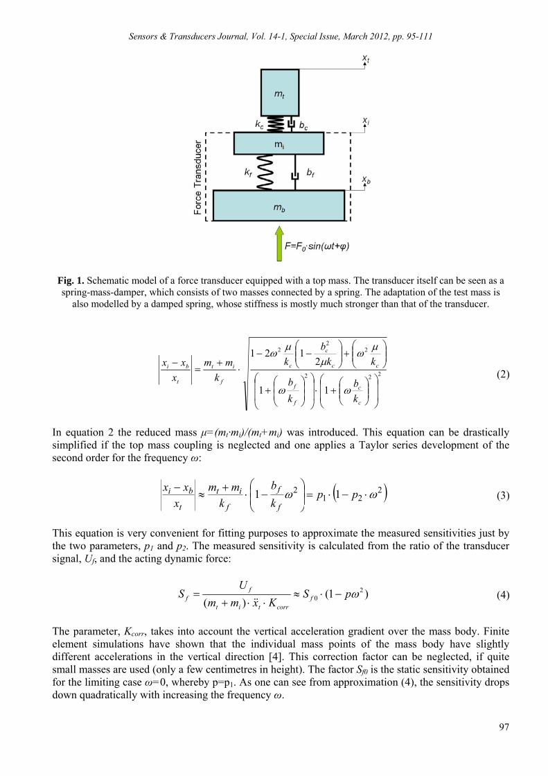
transducers are used in dynamic applications. That is the reason why more and more NMI’s have established procedures for a dynamic calibration of force transducers and also other sensors. Currently in the European Metrology Research Programme (EMRP) one promoted research topic is the: “Traceable Dynamic Measurement of Mechanical Quantities”, which includes, apart from a work package about dynamic force, also work packages about dynamic pressure, dynamic torque, the electrical characterization of measuring amplifiers and mathematical and statistical methods and modelling [3]. Similar to the static calibration philosophy primary calibrations have to be provided which guarantee traceability to the SI base units and also transfer transducers (reference standards) to transfer these calibrations e.g. to an industrial application. This transfer turned out to be the most complicated task because of the crucial influence of environmental conditions present in certain applications. Mostly the transducers are clamped from both sides which lead to sensitivity losses due to the dynamics of these connections which are more or less not infinitely stiff. On the other hand the resonant frequency often shifts down to lower frequencies which can also drastically change the sensitivity. The problem can be solved to a certain extent by modelling the whole construction including all relevant parameters. For that reason it is also important to determine the force transducer parameters like stiffness and damping which can be obtained during a dynamic calibration. This article describes one possibility for a primary dynamic force calibration using sinusoidal excitations. The whole procedure as well as most of the set-ups where developed over two decades and are extensively described in [4]. Other methods as well as analysis procedures for dynamic force calibration are described in [5-9]. 2. Mathematical Description To obtain an analytical “handle” for the description of the dynamic behaviour of a dynamically excited force transducer, the well-known spring-mass-damper model can be applied. In Fig. 1 one can see a simplified picture of a force transducer which is equipped with a test mass, mt. The connection of that mass to the transducer is modelled by a certain stiffness, kc, and a damping constant, bc. The transducer itself consists of a bottom mass, mb, and a head mass, mi. Both masses are also connected by a spring with stiffness, kf, and a corresponding dumping constant, bf. The coordinates in space of all three masses are then given by the vector (xt, xi, xb), if only a vertical movement is considered. A periodical force acts from the bottom on the mass, mb, (see Fig.1). This force is generated by an electrodynamic shaker system. The acceleration of the top mass, tx , the acceleration on the shaker table, bx , and the

force transducer electrical signal are measured during the calibration procedure. This transducer signal is directly proportional to the material tension/compression and can be described in the model by the difference of the spring coordinates xi-xb.

Fxxbxxkxm

xxbxxkxxbxxkxm

xxbxxkxm

bifbifbb

bifbifitcitcii

itcitctt

(1)

It should be noted that the system can be simplified if the coupling of the top mass has practically no influence on the dynamic process. This would correspond to the special case, kc , bc 0, and the top mass as well as the head mass of the transducer can be summarized as one mass body. In the calibration process the dynamic sensitivity, which is the ratio between the measured force transducer signal and the acting dynamic force, is measured as follows:


97

Fig. 1. Schematic model of a force transducer equipped with a top mass. The transducer itself can be seen as a spring-mass-damper, which consists of two masses connected by a spring. The adaptation of the test mass is

also modelled by a damped spring, whose stiffness is mostly much stronger than that of the transducer.

222

22

2

11

2121

c

c

f

f

cc

c

c

f

it

t

bi

k

b

k

b

kk

b

k

k

mm

x

xx

(2)

In equation 2 the reduced mass μ=(mt·mi)/(mt+mi) was introduced. This equation can be drastically simplified if the top mass coupling is neglected and one applies a Taylor series development of the second order for the frequency ω: 2

212 11

pp

k

b

k

mm

x

xx

f

f

f

it

t

bi

(3)

This equation is very convenient for fitting purposes to approximate the measured sensitivities just by the two parameters, p1 and p2. The measured sensitivity is calculated from the ratio of the transducer signal, Uf, and the acting dynamic force:

)1()(

20 pS

Kxmm

US f

corrtit

ff

(4)

The parameter, Kcorr, takes into account the vertical acceleration gradient over the mass body. Finite element simulations have shown that the individual mass points of the mass body have slightly different accelerations in the vertical direction [4]. This correction factor can be neglected, if quite small masses are used (only a few centimetres in height). The factor Sf0 is the static sensitivity obtained for the limiting case ω=0, whereby p=p1. As one can see from approximation (4), the sensitivity drops down quadratically with increasing the frequency ω.


98

Besides the amplitude of the sensitivity according to equation (4), also the phase shift between the acceleration xt and the force signal Uf can be derived by the model:

f

f

f

f

fcfc

fc

f

f

k

b

k

b

bkfbkf

bkf

k

b

1

,32

,24

,12

1

tan)(

),/1(),/1(1

),/1(1tan)(

(5)

The quite complicated equation (5) contains functions f1-f3 which are all proportional to 1/kc , so that these terms can be neglected for the limiting case of infinite coupling stiffness of the top mass. In addition the arcus-tangent function can be approximated by a Taylor series of the first order for the frequency ω, which leads to a linear phase shift between the acceleration- and force transducer signal. Last but not least, the parameters, kf and bf of the force transducer can be determined via a dynamic measurement. So far, the parameter determination was practically accomplished only in a quite simple approach. The model according to Fig. 1 can be simplified in such a way, that it has only one mass, m=m1+m2, connected with a spring, with spring constant, k, and damping factor b, which means that the whole coupling of the top mass is neglected. The bottom mass, m3, of the force transducer can be seen as a fixed part connected with the shaker table. In such a figure, the equation of motion is just given by ftieFkxxbxm 2

0 (6)

The complex output of the force transducer as a function of the frequency, X(f), is then obtained by the product of a complex transfer function, H(f) and the acting dynamic force:

0

2

0

20

11

/1)(

)()(

f

f

Qi

f

f

kfH

eFfHfX fti

(7)

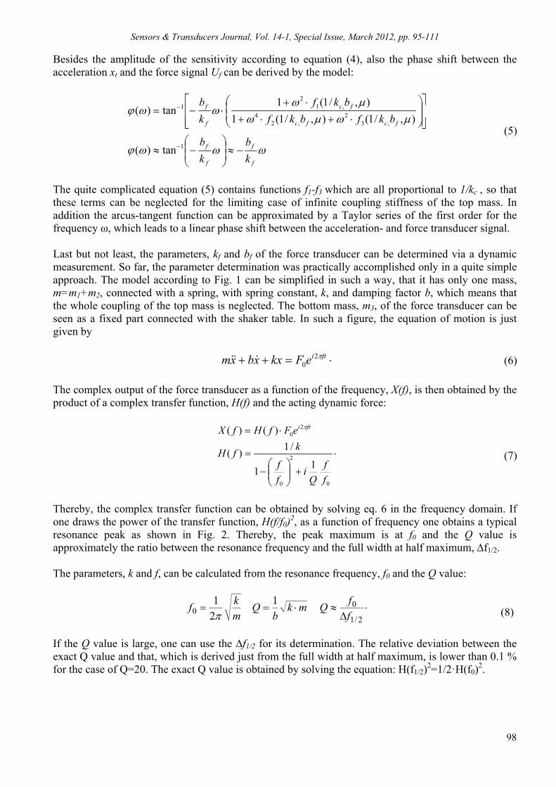
Thereby, the complex transfer function can be obtained by solving eq. 6 in the frequency domain. If one draws the power of the transfer function, H(f/f0)

2, as a function of frequency one obtains a typical resonance peak as shown in Fig. 2. Thereby, the peak maximum is at f0 and the Q value is approximately the ratio between the resonance frequency and the full width at half maximum, ∆f1/2. The parameters, k and f, can be calculated from the resonance frequency, f0 and the Q value:

2/1

00

121

f

fQmk

bQ

mk

f

(8)

If the Q value is large, one can use the ∆f1/2 for its determination. The relative deviation between the exact Q value and that, which is derived just from the full width at half maximum, is lower than 0.1 % for the case of Q=20. The exact Q value is obtained by solving the equation: H(f1/2)

2=1/2·H(f0)2.


99

Fig. 2. Schematic representation of a resonance peak resulting from equation (7). The Q-value represents the quality of the resonance peak, as higher the Q-value as smaller the width of the resonance peak.

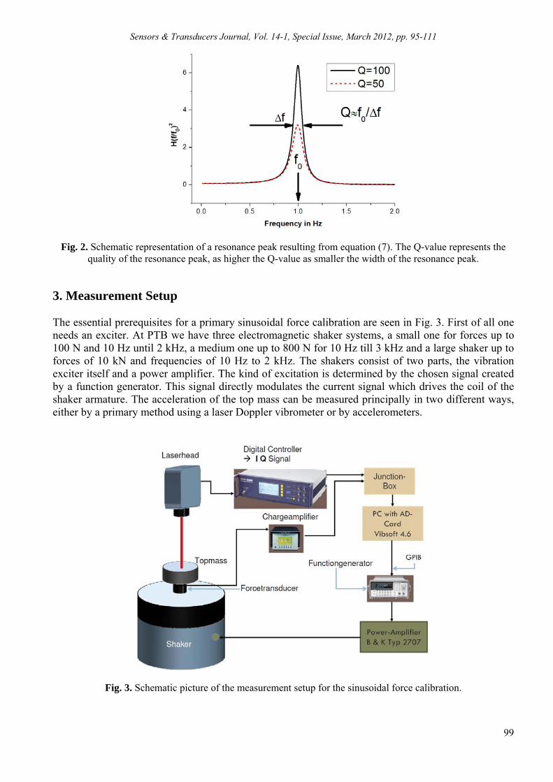
3. Measurement Setup The essential prerequisites for a primary sinusoidal force calibration are seen in Fig. 3. First of all one needs an exciter. At PTB we have three electromagnetic shaker systems, a small one for forces up to 100 N and 10 Hz until 2 kHz, a medium one up to 800 N for 10 Hz till 3 kHz and a large shaker up to forces of 10 kN and frequencies of 10 Hz to 2 kHz. The shakers consist of two parts, the vibration exciter itself and a power amplifier. The kind of excitation is determined by the chosen signal created by a function generator. This signal directly modulates the current signal which drives the coil of the shaker armature. The acceleration of the top mass can be measured principally in two different ways, either by a primary method using a laser Doppler vibrometer or by accelerometers.

Fig. 3. Schematic picture of the measurement setup for the sinusoidal force calibration.


100

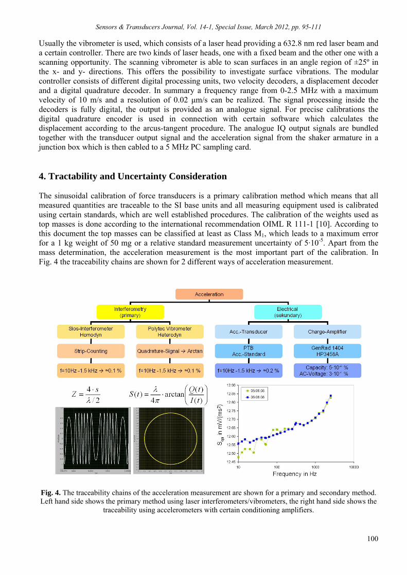
Usually the vibrometer is used, which consists of a laser head providing a 632.8 nm red laser beam and a certain controller. There are two kinds of laser heads, one with a fixed beam and the other one with a scanning opportunity. The scanning vibrometer is able to scan surfaces in an angle region of ±25º in the x- and y- directions. This offers the possibility to investigate surface vibrations. The modular controller consists of different digital processing units, two velocity decoders, a displacement decoder and a digital quadrature decoder. In summary a frequency range from 0-2.5 MHz with a maximum velocity of 10 m/s and a resolution of 0.02 μm/s can be realized. The signal processing inside the decoders is fully digital, the output is provided as an analogue signal. For precise calibrations the digital quadrature encoder is used in connection with certain software which calculates the displacement according to the arcus-tangent procedure. The analogue IQ output signals are bundled together with the transducer output signal and the acceleration signal from the shaker armature in a junction box which is then cabled to a 5 MHz PC sampling card. 4. Tractability and Uncertainty Consideration The sinusoidal calibration of force transducers is a primary calibration method which means that all measured quantities are traceable to the SI base units and all measuring equipment used is calibrated using certain standards, which are well established procedures. The calibration of the weights used as top masses is done according to the international recommendation OIML R 111-1 [10]. According to this document the top masses can be classified at least as Class M1, which leads to a maximum error for a 1 kg weight of 50 mg or a relative standard measurement uncertainty of 5·10-5. Apart from the mass determination, the acceleration measurement is the most important part of the calibration. In Fig. 4 the traceability chains are shown for 2 different ways of acceleration measurement.

Fig. 4. The traceability chains of the acceleration measurement are shown for a primary and secondary method. Left hand side shows the primary method using laser interferometers/vibrometers, the right hand side shows the

traceability using accelerometers with certain conditioning amplifiers.


101

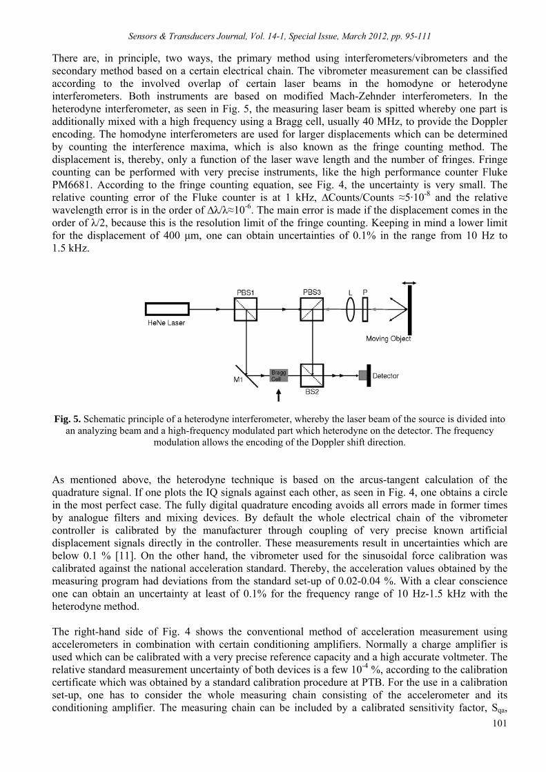
There are, in principle, two ways, the primary method using interferometers/vibrometers and the secondary method based on a certain electrical chain. The vibrometer measurement can be classified according to the involved overlap of certain laser beams in the homodyne or heterodyne interferometers. Both instruments are based on modified Mach-Zehnder interferometers. In the heterodyne interferometer, as seen in Fig. 5, the measuring laser beam is spitted whereby one part is additionally mixed with a high frequency using a Bragg cell, usually 40 MHz, to provide the Doppler encoding. The homodyne interferometers are used for larger displacements which can be determined by counting the interference maxima, which is also known as the fringe counting method. The displacement is, thereby, only a function of the laser wave length and the number of fringes. Fringe counting can be performed with very precise instruments, like the high performance counter Fluke PM6681. According to the fringe counting equation, see Fig. 4, the uncertainty is very small. The relative counting error of the Fluke counter is at 1 kHz, ∆Counts/Counts ≈5·10-8 and the relative wavelength error is in the order of ∆λ/λ≈10-6. The main error is made if the displacement comes in the order of λ/2, because this is the resolution limit of the fringe counting. Keeping in mind a lower limit for the displacement of 400 μm, one can obtain uncertainties of 0.1% in the range from 10 Hz to 1.5 kHz.

Fig. 5. Schematic principle of a heterodyne interferometer, whereby the laser beam of the source is divided into an analyzing beam and a high-frequency modulated part which heterodyne on the detector. The frequency

modulation allows the encoding of the Doppler shift direction.

As mentioned above, the heterodyne technique is based on the arcus-tangent calculation of the quadrature signal. If one plots the IQ signals against each other, as seen in Fig. 4, one obtains a circle in the most perfect case. The fully digital quadrature encoding avoids all errors made in former times by analogue filters and mixing devices. By default the whole electrical chain of the vibrometer controller is calibrated by the manufacturer through coupling of very precise known artificial displacement signals directly in the controller. These measurements result in uncertainties which are below 0.1 % [11]. On the other hand, the vibrometer used for the sinusoidal force calibration was calibrated against the national acceleration standard. Thereby, the acceleration values obtained by the measuring program had deviations from the standard set-up of 0.02-0.04 %. With a clear conscience one can obtain an uncertainty at least of 0.1% for the frequency range of 10 Hz-1.5 kHz with the heterodyne method. The right-hand side of Fig. 4 shows the conventional method of acceleration measurement using accelerometers in combination with certain conditioning amplifiers. Normally a charge amplifier is used which can be calibrated with a very precise reference capacity and a high accurate voltmeter. The relative standard measurement uncertainty of both devices is a few 10-4 %, according to the calibration certificate which was obtained by a standard calibration procedure at PTB. For the use in a calibration set-up, one has to consider the whole measuring chain consisting of the accelerometer and its conditioning amplifier. The measuring chain can be included by a calibrated sensitivity factor, Sqa,


102

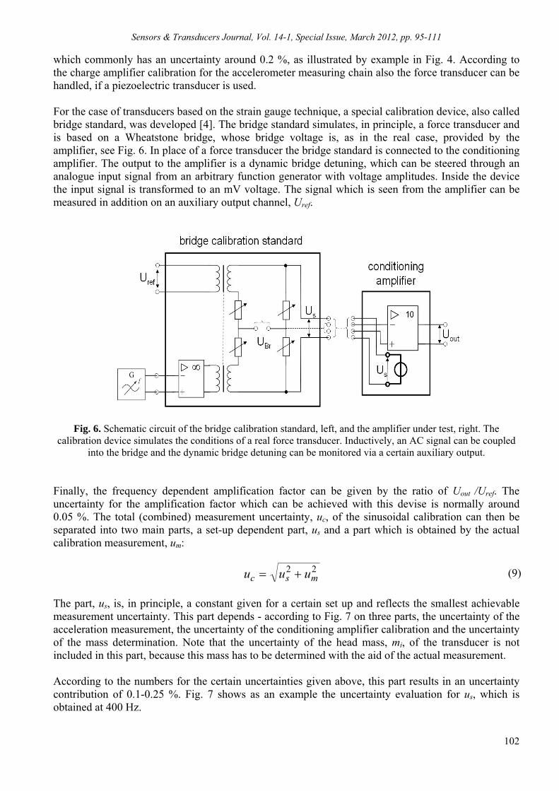
which commonly has an uncertainty around 0.2 %, as illustrated by example in Fig. 4. According to the charge amplifier calibration for the accelerometer measuring chain also the force transducer can be handled, if a piezoelectric transducer is used. For the case of transducers based on the strain gauge technique, a special calibration device, also called bridge standard, was developed [4]. The bridge standard simulates, in principle, a force transducer and is based on a Wheatstone bridge, whose bridge voltage is, as in the real case, provided by the amplifier, see Fig. 6. In place of a force transducer the bridge standard is connected to the conditioning amplifier. The output to the amplifier is a dynamic bridge detuning, which can be steered through an analogue input signal from an arbitrary function generator with voltage amplitudes. Inside the device the input signal is transformed to an mV voltage. The signal which is seen from the amplifier can be measured in addition on an auxiliary output channel, Uref.

Fig. 6. Schematic circuit of the bridge calibration standard, left, and the amplifier under test, right. The calibration device simulates the conditions of a real force transducer. Inductively, an AC signal can be coupled

into the bridge and the dynamic bridge detuning can be monitored via a certain auxiliary output. Finally, the frequency dependent amplification factor can be given by the ratio of Uout /Uref. The uncertainty for the amplification factor which can be achieved with this devise is normally around 0.05 %. The total (combined) measurement uncertainty, uc, of the sinusoidal calibration can then be separated into two main parts, a set-up dependent part, us and a part which is obtained by the actual calibration measurement, um: 22

msc uuu (9)

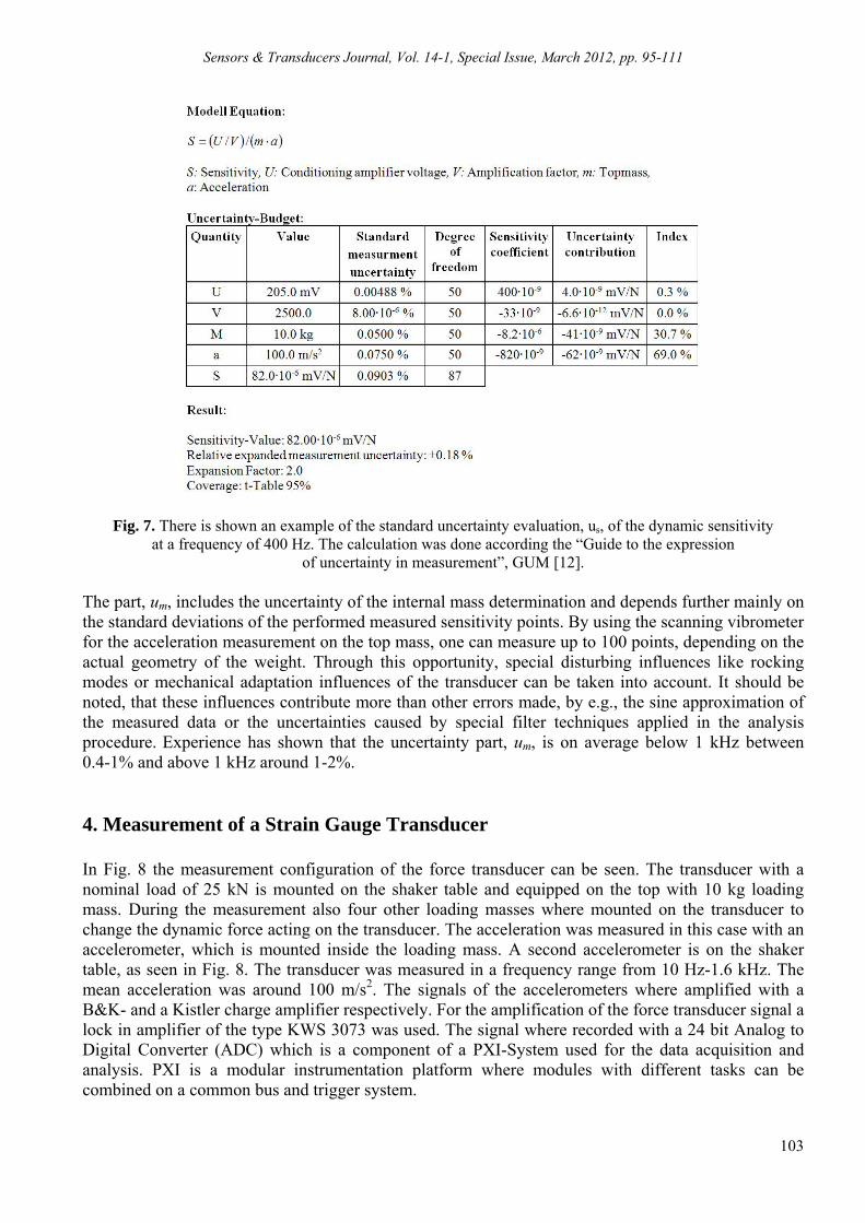
The part, us, is, in principle, a constant given for a certain set up and reflects the smallest achievable measurement uncertainty. This part depends - according to Fig. 7 on three parts, the uncertainty of the acceleration measurement, the uncertainty of the conditioning amplifier calibration and the uncertainty of the mass determination. Note that the uncertainty of the head mass, mi, of the transducer is not included in this part, because this mass has to be determined with the aid of the actual measurement. According to the numbers for the certain uncertainties given above, this part results in an uncertainty contribution of 0.1-0.25 %. Fig. 7 shows as an example the uncertainty evaluation for us, which is obtained at 400 Hz.


103

Fig. 7. There is shown an example of the standard uncertainty evaluation, us, of the dynamic sensitivity at a frequency of 400 Hz. The calculation was done according the “Guide to the expression

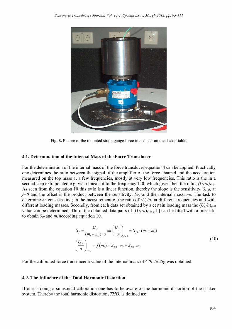
of uncertainty in measurement”, GUM [12]. The part, um, includes the uncertainty of the internal mass determination and depends further mainly on the standard deviations of the performed measured sensitivity points. By using the scanning vibrometer for the acceleration measurement on the top mass, one can measure up to 100 points, depending on the actual geometry of the weight. Through this opportunity, special disturbing influences like rocking modes or mechanical adaptation influences of the transducer can be taken into account. It should be noted, that these influences contribute more than other errors made, by e.g., the sine approximation of the measured data or the uncertainties caused by special filter techniques applied in the analysis procedure. Experience has shown that the uncertainty part, um, is on average below 1 kHz between 0.4-1% and above 1 kHz around 1-2%. 4. Measurement of a Strain Gauge Transducer In Fig. 8 the measurement configuration of the force transducer can be seen. The transducer with a nominal load of 25 kN is mounted on the shaker table and equipped on the top with 10 kg loading mass. During the measurement also four other loading masses where mounted on the transducer to change the dynamic force acting on the transducer. The acceleration was measured in this case with an accelerometer, which is mounted inside the loading mass. A second accelerometer is on the shaker table, as seen in Fig. 8. The transducer was measured in a frequency range from 10 Hz-1.6 kHz. The mean acceleration was around 100 m/s2. The signals of the accelerometers where amplified with a B&K- and a Kistler charge amplifier respectively. For the amplification of the force transducer signal a lock in amplifier of the type KWS 3073 was used. The signal where recorded with a 24 bit Analog to Digital Converter (ADC) which is a component of a PXI-System used for the data acquisition and analysis. PXI is a modular instrumentation platform where modules with different tasks can be combined on a common bus and trigger system.


104

Fig. 8. Picture of the mounted strain gauge force transducer on the shaker table.

4.1. Determination of the Internal Mass of the Force Transducer For the determination of the internal mass of the force transducer equation 4 can be applied. Practically one determines the ratio between the signal of the amplifier of the force channel and the acceleration measured on the top mass at a few frequencies, mostly at very low frequencies. This ratio is the in a second step extrapolated e.g. via a linear fit to the frequency f=0, which gives then the ratio, (Uf /a)f=0. As seen from the equation 10 this ratio is a linear function, thereby the slope is the sensitivity, Sf=0, at f=0 and the offset is the product between the sensitivity, Sf0, and the internal mass, mi. The task to determine mi consists first; in the measurement of the ratio of (Uf /a) at different frequencies and with different loading masses. Secondly, from each data set obtained by a certain loading mass the (Uf /a)f=0 value can be determined. Third, the obtained data pairs of [(Uf /a)f=0 , f ] can be fitted with a linear fit to obtain Sf0 and mi according equation 10.

iftft

f

f

itf

f

f

it

ff

mSmSmfa

U

mmSa

U

amm

US

00

0

0

0

)(

)()(

(10)

For the calibrated force transducer a value of the internal mass of 479.7±25g was obtained. 4.2. The Influence of the Total Harmonic Distortion If one is doing a sinusoidal calibration one has to be aware of the harmonic distortion of the shaker system. Thereby the total harmonic distortion, THD, is defined as:


105

1

223

22

A

AAATHD N

(11)

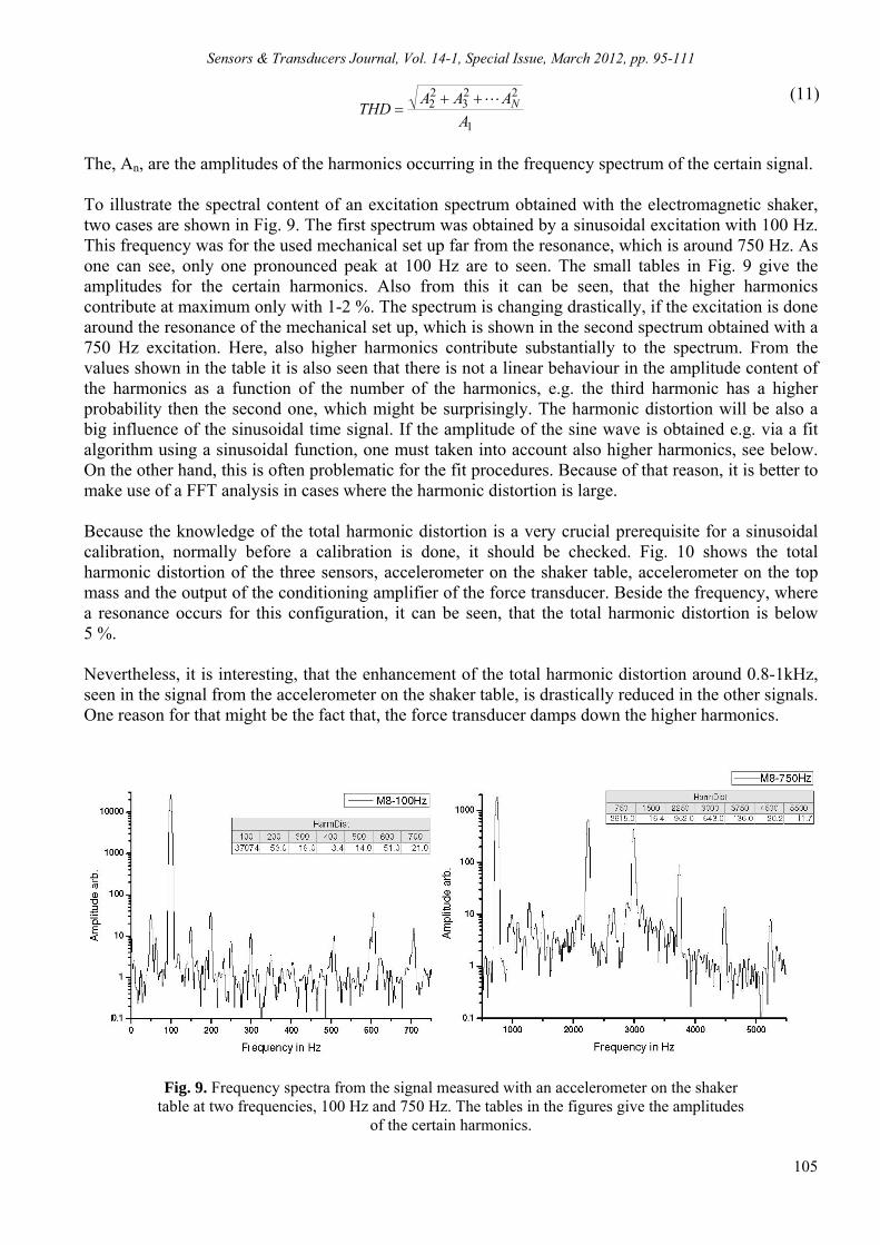
The, An, are the amplitudes of the harmonics occurring in the frequency spectrum of the certain signal. To illustrate the spectral content of an excitation spectrum obtained with the electromagnetic shaker, two cases are shown in Fig. 9. The first spectrum was obtained by a sinusoidal excitation with 100 Hz. This frequency was for the used mechanical set up far from the resonance, which is around 750 Hz. As one can see, only one pronounced peak at 100 Hz are to seen. The small tables in Fig. 9 give the amplitudes for the certain harmonics. Also from this it can be seen, that the higher harmonics contribute at maximum only with 1-2 %. The spectrum is changing drastically, if the excitation is done around the resonance of the mechanical set up, which is shown in the second spectrum obtained with a 750 Hz excitation. Here, also higher harmonics contribute substantially to the spectrum. From the values shown in the table it is also seen that there is not a linear behaviour in the amplitude content of the harmonics as a function of the number of the harmonics, e.g. the third harmonic has a higher probability then the second one, which might be surprisingly. The harmonic distortion will be also a big influence of the sinusoidal time signal. If the amplitude of the sine wave is obtained e.g. via a fit algorithm using a sinusoidal function, one must taken into account also higher harmonics, see below. On the other hand, this is often problematic for the fit procedures. Because of that reason, it is better to make use of a FFT analysis in cases where the harmonic distortion is large. Because the knowledge of the total harmonic distortion is a very crucial prerequisite for a sinusoidal calibration, normally before a calibration is done, it should be checked. Fig. 10 shows the total harmonic distortion of the three sensors, accelerometer on the shaker table, accelerometer on the top mass and the output of the conditioning amplifier of the force transducer. Beside the frequency, where a resonance occurs for this configuration, it can be seen, that the total harmonic distortion is below 5 %. Nevertheless, it is interesting, that the enhancement of the total harmonic distortion around 0.8-1kHz, seen in the signal from the accelerometer on the shaker table, is drastically reduced in the other signals. One reason for that might be the fact that, the force transducer damps down the higher harmonics.

Fig. 9. Frequency spectra from the signal measured with an accelerometer on the shaker table at two frequencies, 100 Hz and 750 Hz. The tables in the figures give the amplitudes

of the certain harmonics.


106

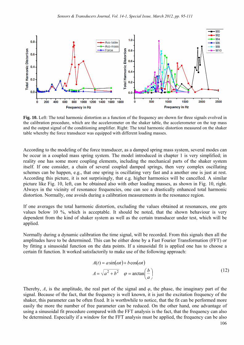
Fig. 10. Left: The total harmonic distortion as a function of the frequency are shown for three signals evolved in the calibration procedure, which are the accelerometer on the shaker table, the accelerometer on the top mass and the output signal of the conditioning amplifier. Right: The total harmonic distortion measured on the shaker table whereby the force transducer was equipped with different loading masses.

According to the modeling of the force transducer, as a damped spring mass system, several modes can be occur in a coupled mass spring system. The model introduced in chapter 1 is very simplified; in reality one has some more coupling elements, including the mechanical parts of the shaker system itself. If one consider, a chain of several coupled damped springs, then very complex oscillating schemes can be happen, e.g., that one spring is oscillating very fast and a another one is just at rest. According this picture, it is not surprisingly, that e.g. higher harmonics will be cancelled. A similar picture like Fig. 10, left, can be obtained also with other loading masses, as shown in Fig. 10, right. Always in the vicinity of resonance frequencies, one can see a drastically enhanced total harmonic distortion. Normally, one avoids during a calibration measurements in the resonance region. If one averages the total harmonic distortion, excluding the values obtained at resonances, one gets values below 10 %, which is acceptable. It should be noted, that the shown behaviour is very dependent from the kind of shaker system as well as the certain transducer under test, which will be applied.

Normally during a dynamic calibration the time signal, will be recorded. From this signals then all the amplitudes have to be determined. This can be either done by a Fast Fourier Transformation (FFT) or by fitting a sinusoidal function on the data points. If a sinusoidal fit is applied one has to choose a certain fit function. It worked satisfactorily to make use of the following approach:

a

bbaA

tbtatA

arctan

cossin)(

22

(12)

Thereby, A, is the amplitude, the real part of the signal and φ, the phase, the imaginary part of the signal. Because of the fact, that the frequency is well known, it is just the excitation frequency of the shaker, this parameter can be often fixed. It is worthwhile to notice, that the fit can be performed more easily the more the number of free parameter can be reduced. On the other hand, one advantage of using a sinusoidal fit procedure compared with the FFT analysis is the fact, that the frequency can also be determined. Especially if a window for the FFT analysis must be applied, the frequency can be also


107

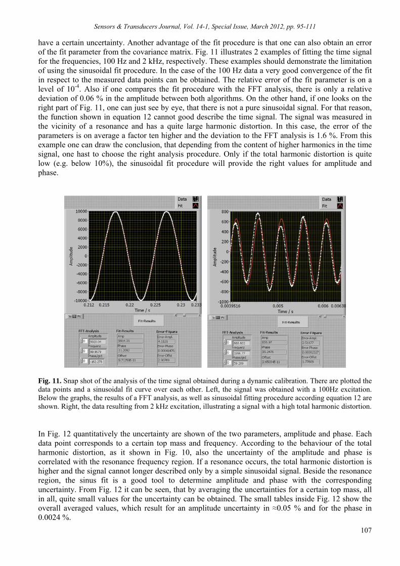
have a certain uncertainty. Another advantage of the fit procedure is that one can also obtain an error of the fit parameter from the covariance matrix. Fig. 11 illustrates 2 examples of fitting the time signal for the frequencies, 100 Hz and 2 kHz, respectively. These examples should demonstrate the limitation of using the sinusoidal fit procedure. In the case of the 100 Hz data a very good convergence of the fit in respect to the measured data points can be obtained. The relative error of the fit parameter is on a level of 10-4. Also if one compares the fit procedure with the FFT analysis, there is only a relative deviation of 0.06 % in the amplitude between both algorithms. On the other hand, if one looks on the right part of Fig. 11, one can just see by eye, that there is not a pure sinusoidal signal. For that reason, the function shown in equation 12 cannot good describe the time signal. The signal was measured in the vicinity of a resonance and has a quite large harmonic distortion. In this case, the error of the parameters is on average a factor ten higher and the deviation to the FFT analysis is 1.6 %. From this example one can draw the conclusion, that depending from the content of higher harmonics in the time signal, one hast to choose the right analysis procedure. Only if the total harmonic distortion is quite low (e.g. below 10%), the sinusoidal fit procedure will provide the right values for amplitude and phase.

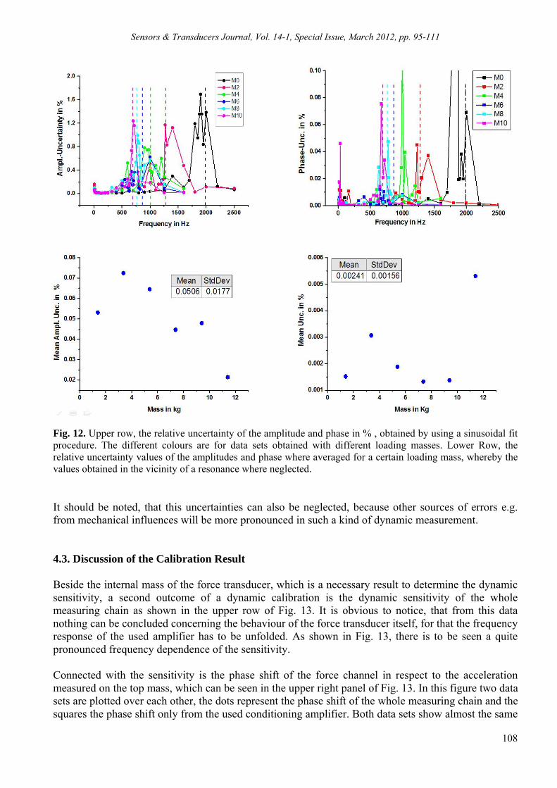
Fig. 11. Snap shot of the analysis of the time signal obtained during a dynamic calibration. There are plotted the data points and a sinusoidal fit curve over each other. Left, the signal was obtained with a 100Hz excitation. Below the graphs, the results of a FFT analysis, as well as sinusoidal fitting procedure according equation 12 are shown. Right, the data resulting from 2 kHz excitation, illustrating a signal with a high total harmonic distortion. In Fig. 12 quantitatively the uncertainty are shown of the two parameters, amplitude and phase. Each data point corresponds to a certain top mass and frequency. According to the behaviour of the total harmonic distortion, as it shown in Fig. 10, also the uncertainty of the amplitude and phase is correlated with the resonance frequency region. If a resonance occurs, the total harmonic distortion is higher and the signal cannot longer described only by a simple sinusoidal signal. Beside the resonance region, the sinus fit is a good tool to determine amplitude and phase with the corresponding uncertainty. From Fig. 12 it can be seen, that by averaging the uncertainties for a certain top mass, all in all, quite small values for the uncertainty can be obtained. The small tables inside Fig. 12 show the overall averaged values, which result for an amplitude uncertainty in ≈0.05 % and for the phase in 0.0024 %.


108

Fig. 12. Upper row, the relative uncertainty of the amplitude and phase in % , obtained by using a sinusoidal fit procedure. The different colours are for data sets obtained with different loading masses. Lower Row, the relative uncertainty values of the amplitudes and phase where averaged for a certain loading mass, whereby the values obtained in the vicinity of a resonance where neglected.

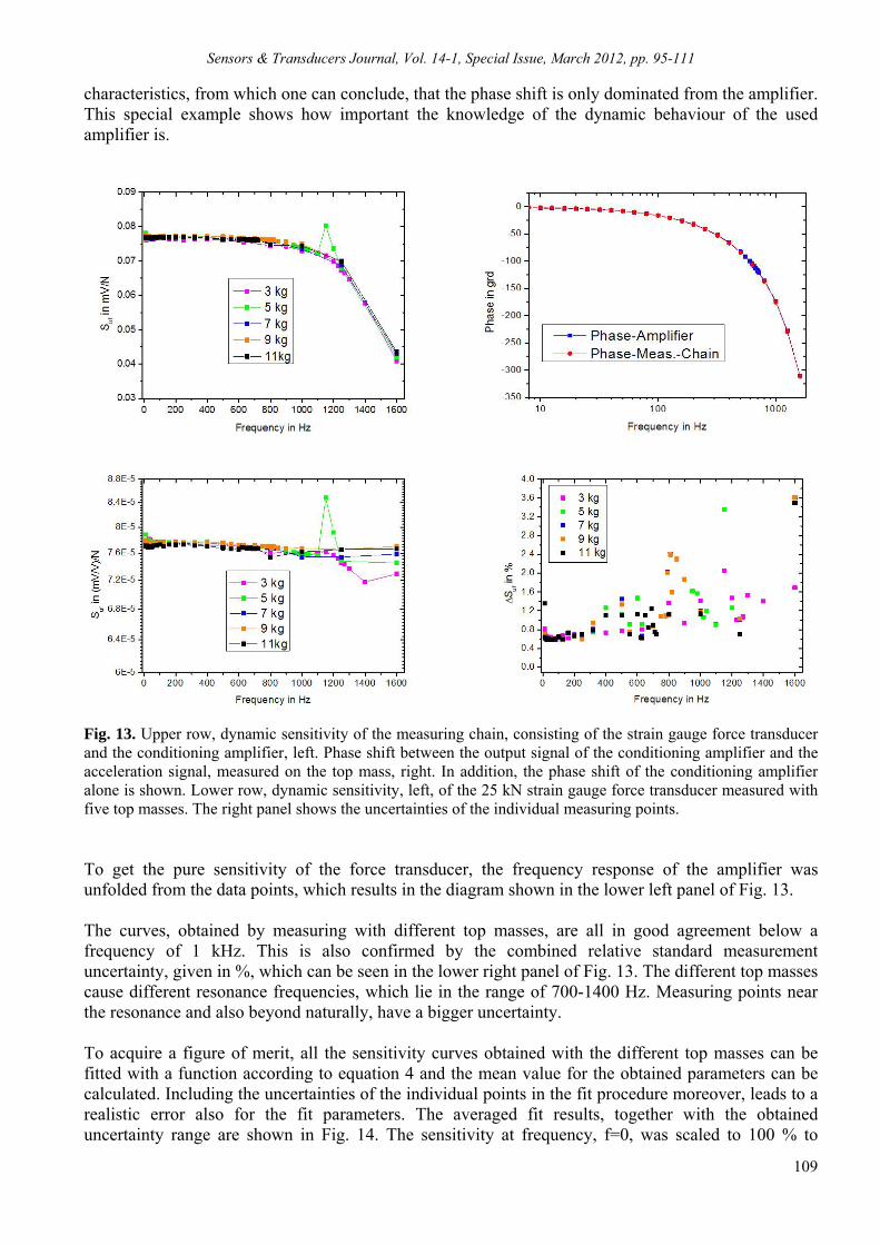
It should be noted, that this uncertainties can also be neglected, because other sources of errors e.g. from mechanical influences will be more pronounced in such a kind of dynamic measurement. 4.3. Discussion of the Calibration Result Beside the internal mass of the force transducer, which is a necessary result to determine the dynamic sensitivity, a second outcome of a dynamic calibration is the dynamic sensitivity of the whole measuring chain as shown in the upper row of Fig. 13. It is obvious to notice, that from this data nothing can be concluded concerning the behaviour of the force transducer itself, for that the frequency response of the used amplifier has to be unfolded. As shown in Fig. 13, there is to be seen a quite pronounced frequency dependence of the sensitivity. Connected with the sensitivity is the phase shift of the force channel in respect to the acceleration measured on the top mass, which can be seen in the upper right panel of Fig. 13. In this figure two data sets are plotted over each other, the dots represent the phase shift of the whole measuring chain and the squares the phase shift only from the used conditioning amplifier. Both data sets show almost the same


109

characteristics, from which one can conclude, that the phase shift is only dominated from the amplifier. This special example shows how important the knowledge of the dynamic behaviour of the used amplifier is.

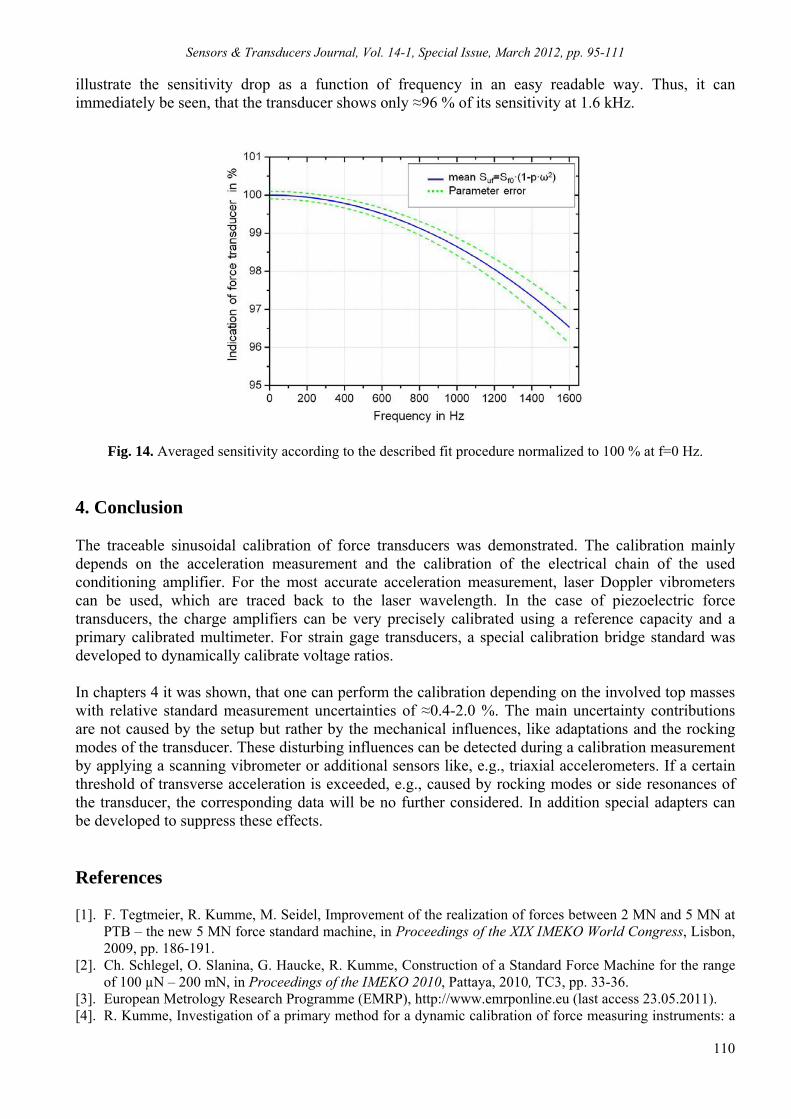
Fig. 13. Upper row, dynamic sensitivity of the measuring chain, consisting of the strain gauge force transducer and the conditioning amplifier, left. Phase shift between the output signal of the conditioning amplifier and the acceleration signal, measured on the top mass, right. In addition, the phase shift of the conditioning amplifier alone is shown. Lower row, dynamic sensitivity, left, of the 25 kN strain gauge force transducer measured with five top masses. The right panel shows the uncertainties of the individual measuring points. To get the pure sensitivity of the force transducer, the frequency response of the amplifier was unfolded from the data points, which results in the diagram shown in the lower left panel of Fig. 13. The curves, obtained by measuring with different top masses, are all in good agreement below a frequency of 1 kHz. This is also confirmed by the combined relative standard measurement uncertainty, given in %, which can be seen in the lower right panel of Fig. 13. The different top masses cause different resonance frequencies, which lie in the range of 700-1400 Hz. Measuring points near the resonance and also beyond naturally, have a bigger uncertainty. To acquire a figure of merit, all the sensitivity curves obtained with the different top masses can be fitted with a function according to equation 4 and the mean value for the obtained parameters can be calculated. Including the uncertainties of the individual points in the fit procedure moreover, leads to a realistic error also for the fit parameters. The averaged fit results, together with the obtained uncertainty range are shown in Fig. 14. The sensitivity at frequency, f=0, was scaled to 100 % to


110

illustrate the sensitivity drop as a function of frequency in an easy readable way. Thus, it can immediately be seen, that the transducer shows only ≈96 % of its sensitivity at 1.6 kHz.

Fig. 14. Averaged sensitivity according to the described fit procedure normalized to 100 % at f=0 Hz. 4. Conclusion The traceable sinusoidal calibration of force transducers was demonstrated. The calibration mainly depends on the acceleration measurement and the calibration of the electrical chain of the used conditioning amplifier. For the most accurate acceleration measurement, laser Doppler vibrometers can be used, which are traced back to the laser wavelength. In the case of piezoelectric force transducers, the charge amplifiers can be very precisely calibrated using a reference capacity and a primary calibrated multimeter. For strain gage transducers, a special calibration bridge standard was developed to dynamically calibrate voltage ratios. In chapters 4 it was shown, that one can perform the calibration depending on the involved top masses with relative standard measurement uncertainties of ≈0.4-2.0 %. The main uncertainty contributions are not caused by the setup but rather by the mechanical influences, like adaptations and the rocking modes of the transducer. These disturbing influences can be detected during a calibration measurement by applying a scanning vibrometer or additional sensors like, e.g., triaxial accelerometers. If a certain threshold of transverse acceleration is exceeded, e.g., caused by rocking modes or side resonances of the transducer, the corresponding data will be no further considered. In addition special adapters can be developed to suppress these effects. References [1]. F. Tegtmeier, R. Kumme, M. Seidel, Improvement of the realization of forces between 2 MN and 5 MN at

PTB – the new 5 MN force standard machine, in Proceedings of the XIX IMEKO World Congress, Lisbon, 2009, pp. 186-191.

[2]. Ch. Schlegel, O. Slanina, G. Haucke, R. Kumme, Construction of a Standard Force Machine for the range of 100 µN – 200 mN, in Proceedings of the IMEKO 2010, Pattaya, 2010, TC3, pp. 33-36.

[3]. European Metrology Research Programme (EMRP), http://www.emrponline.eu (last access 23.05.2011). [4]. R. Kumme, Investigation of a primary method for a dynamic calibration of force measuring instruments: a


111

contribution to reduce the measuring uncertainty, Doctoral Thesis (in German), PTB, 1996. [5]. S. Eichstädt, C. Elster, T. J. Esward and J. P. Hessling, Deconvolution filters for the analysis of dynamic

measurement processes: a tutorial, Metrologia, 47, 2010, pp. 522-533. [6]. G. Wegener and Th. Bruns, Traceability of torque transducers under rotating and dynamic operating con-

ditions, 2009, Measurement, 42, pp. 1448-1453. [7]. M. Kobusch, Th. Bruns and E. Franke, Challenges in Practical Dynamic Calibration, Advanced

Mathematical and Computational Tools in Metrology and Testing, edited by Franco Pavese, Series on Advances in Mathematics for Applied Sciences, World Scientific Publishing, Singapore, Vol. 78, 2009, pp. 204-212.

[8]. C. Elster and A. Link, Uncertainty evaluation for dynamic measurements modelled by a linear time- invariant system, Metrologia, 2008, 45, pp. 464-473.

[9]. M. Kobusch, The 250 kN primary shock force calibration device at PTB, in Proceedings of the IMEKO 2010, TC3, Thailand, Pattaya, November 2010.

[10]. International Recommendation, OIML R 111-1, International Organization of Legal Metrology, 2004. [11]. G. Siegmund, Sources of Measurement Error in Laser Doppler Vibrometers and Proposal for Unified

Specifications, in Proceedings of the 8th. SPIE Int. Conf. on Vibration Measurements by Laser Techniques, Vol. 70980Y, 2008.

[12]. ISO/IEC Guide 98-3:2008: Uncertainty of measurement – Part3: Guide to the expression of uncertainty in measurement. ISO, Genf 2008.

___________________ 2012 Copyright ©, International Frequency Sensor Association (IFSA). All rights reserved. (http://www.sensorsportal.com)

http://www.sensorsportal.com/HTML/BOOKSTORE/Smart_Sensors_and_MEMS.htm

Sensors & Transducers Journal

Guide for Contributors

Aims and Scope Sensors & Transducers Journal (ISSN 1726-5479) provides an advanced forum for the science and technology of physical, chemical sensors and biosensors. It publishes state-of-the-art reviews, regular research and application specific papers, short notes, letters to Editor and sensors related books reviews as well as academic, practical and commercial information of interest to its readership. Because of it is a peer reviewed international journal, papers rapidly published in Sensors & Transducers Journal will receive a very high publicity. The journal is published monthly as twelve issues per year by International Frequency Sensor Association (IFSA). In additional, some special sponsored and conference issues published annually. Sensors & Transducers Journal is indexed and abstracted very quickly by Chemical Abstracts, IndexCopernicus Journals Master List, Open J-Gate, Google Scholar, etc. Since 2011 the journal is covered and indexed (including a Scopus, Embase, Engineering Village and Reaxys) in Elsevier products. Topics Covered Contributions are invited on all aspects of research, development and application of the science and technology of sensors, transducers and sensor instrumentations. Topics include, but are not restricted to:

Physical, chemical and biosensors; Digital, frequency, period, duty-cycle, time interval, PWM, pulse number output sensors and

transducers; Theory, principles, effects, design, standardization and modeling; Smart sensors and systems; Sensor instrumentation; Virtual instruments; Sensors interfaces, buses and networks; Signal processing; Frequency (period, duty-cycle)-to-digital converters, ADC; Technologies and materials; Nanosensors; Microsystems; Applications.

Submission of papers Articles should be written in English. Authors are invited to submit by e-mail [email protected] 8-14 pages article (including abstract, illustrations (color or grayscale), photos and references) in both: MS Word (doc) and Acrobat (pdf) formats. Detailed preparation instructions, paper example and template of manuscript are available from the journal’s webpage: http://www.sensorsportal.com/HTML/DIGEST/Submition.htm Authors must follow the instructions strictly when submitting their manuscripts. Advertising Information Advertising orders and enquires may be sent to [email protected] Please download also our media kit: http://www.sensorsportal.com/DOWNLOADS/Media_Kit_2012.pdf


http://www.sensorsportal.com/HTML/BOOKSTORE/Digital_Sensors.htm

sensors & transducers · sensors & transducers volume 14-1, ... mekid, samir, university of...

Documents