september 2017 numerical methods cfd simulations of two ... · calculation of the surface tension...

25 Feb 2016

Numerical Methods in Heat Transfer

Lecture 1 – Review of heat conduction

Mirco Magnini

Certosa di Pontignano, 4th-8th September 2017

CFD simulations of two-phase flows with interface

tracking techniques17th UIT Summer School

Mirco Magnini

UIT Summer School 2017

2

Post-doc research assistant at EPFL; teacher

of Numerical Methods in Heat Transfer (MSc-ME)

Laboratory of Heat and Mass Transfer (LTCM),

director: Prof. John R. Thome

Research interests/activity:

• Numerical simulation of interfacial flows

• Phase change

• Microscale flows

• User/developer of ANSYS Fluent and OpenFOAM

• Theoretical and mechanistic modelling of microscale boiling flows

My background


3

Methods without interface tracking

Numerical representation of an interface between immiscible fluids

Introduction to methods with interface tracking (FT, LS, VOF)

Advection of the volume fraction in VOF

Calculation of the surface tension force in VOF

Phase change models in VOF

Selected CFD studies

Outline


4

CFD methods for gas-liquid and liquid-liquid two-phase flows

A rule of thumb for the choice of the numerical treatment of the interface.

Introduction

𝑎𝑎𝑎𝑎𝑎𝑎𝑎𝑎 𝑜𝑜𝑜𝑜 𝑡𝑡𝑡𝑎𝑎 𝑖𝑖𝑖𝑖𝑡𝑡𝑎𝑎𝑎𝑎𝑜𝑜𝑎𝑎𝑖𝑖𝑎𝑎𝑣𝑣𝑜𝑜𝑣𝑣𝑣𝑣𝑣𝑣𝑎𝑎 𝑜𝑜𝑜𝑜 𝑡𝑡𝑡𝑎𝑎 𝑑𝑑𝑜𝑜𝑣𝑣𝑎𝑎𝑖𝑖𝑖𝑖

Low High

Methods without interface tracking

Eulerian-Lagrangian

Eulerian-Eulerian

Methods with interface tracking

Front Tracking

Level Set

Volume Of Fluid

Moving mesh

Bubbly flowsSlug flows

Annular flowsFilms

Sea waves

Bubbly flowsSpraysMists

Fluidized bedsHomogeneous flows


5

The flow equations for the continuous phase are solved on the Eulerian mesh.

The flow equations for the dispersed phase are solved in Lagrangian manner.

Each unit composing the dispersed phase, e.g. particle, droplet, bubble, is treated separately,

so that a set of flow equations is solved for each unit:

Eulerian-Lagrangian method

𝜌𝜌𝑝𝑝𝜋𝜋𝑑𝑑𝑝𝑝3

6𝑑𝑑𝒖𝒖𝒑𝒑𝑑𝑑𝑡𝑡

= �𝑖𝑖

𝑭𝑭𝒊𝒊 𝒙𝒙, 𝑡𝑡

𝜌𝜌𝑝𝑝𝑖𝑖𝑝𝑝𝜋𝜋𝑑𝑑𝑝𝑝3

6𝑑𝑑𝑇𝑇𝑝𝑝𝑑𝑑𝑡𝑡

= �𝑖𝑖

𝑄𝑄𝑖𝑖 𝒙𝒙, 𝑡𝑡

Coupling between continuous and dispersed phases [1]

This method is suitable for:

• Known shape of the units.

• Low volume fraction of the dispersed phase.

• Negligible particle-particle interactions.

[1] ANSYS Fluent Guide.


6

Eulerian-Lagrangian methodSeparation of gross tobacco fibers by using drag forces and controlled rebounds

Air inlet

Introduction of tobacco fibers with a given inlet velocity

Particles bouncing against the wall

Air and light tobacco fibers leaving the channel

Heavy tobacco fibers falling and exiting the channel Legend

• Lines: trajectory of the

tobacco fibers;

• Colors: speed of the fibers.


7

Eulerian-Eulerian method

[1] M. Z. Podowski and R. M. Podowski, Science and Technology of Nuclear Installations (2009) 387020.

Also known as two-fluid model: the two phases are treated as interpenetrating continua, both

filling up the entire domain.

One set of ensemble-averaged conservation equations is solved for each k-th phase [1]:

net mass transfer rate

totalinterfacial

force

interfacial heat transfer rate

𝛼𝛼𝑘𝑘: volume fraction

Suitable for:

• Well mixed phases.

• High volume fractions.

But:

• Accuracy depends on closure relationships.

• Closure models are problem dependent.


8

Treatment of the interface in CFD

[1] V. P. Carey, Liquid-Vapor Phase Change Phenomena (1992).

Microscopic standpoint: the liquid-vapor interface is a finite

thickness region where fluid properties change continuously

from one phase to the other.

Thickness of the interfacial region ~ 10-9 m.

Macroscopic standpoint: the interface is a massless surface

of vanishing thickness where fluid properties change abruptly.

CFD traditionally adopts the macroscopic standpoint.

Intermolecular forces are modelled by retaining their most important macroscopic effects:

• Surface tension σ: net tension force acting among molecules in the interface region,

parallel to the interface, due to the increased mean molecular spacing.

• Vaporization latent heat hlv: energy necessary to move closely spaced liquid molecules

apart, against attractive forces.

Schematic representation of the molecular density variation in the interfacial region [1]


9

Mass transport at the interface


Mass transport across a control volume moving with the interface [1]:

Interface velocity𝑑𝑑𝑍𝑍𝑖𝑖𝑑𝑑𝑡𝑡

Liquid mass flow rate toward the CV

𝜌𝜌𝑙𝑙 𝑤𝑤𝑙𝑙,𝑛𝑛 −𝑑𝑑𝑍𝑍𝑖𝑖𝑑𝑑𝑡𝑡

𝑑𝑑𝐴𝐴𝑖𝑖

Vapor mass flow rate toward the CV𝜌𝜌𝑣𝑣 𝑤𝑤𝑣𝑣,𝑛𝑛 −

𝑑𝑑𝑍𝑍𝑖𝑖𝑑𝑑𝑡𝑡


Normal velocity jump condition at interface𝜌𝜌𝑙𝑙 𝑤𝑤𝑙𝑙,𝑛𝑛 −𝑑𝑑𝑍𝑍𝑖𝑖𝑑𝑑𝑡𝑡

= 𝜌𝜌𝑣𝑣 𝑤𝑤𝑣𝑣,𝑛𝑛 −𝑑𝑑𝑍𝑍𝑖𝑖𝑑𝑑𝑡𝑡

= 𝑣𝑣𝑖𝑖′′

If normal velocities at the interface are continuous𝑣𝑣𝑖𝑖′′ = 0 ⟹


= 𝑤𝑤𝑙𝑙,𝑛𝑛 = 𝑤𝑤𝑣𝑣,𝑛𝑛

𝑣𝑣𝑖𝑖′′: mass flux at the interface due to phase change [kg/(m2s)]


10

Momentum transport at the interface


Momentum transport normal to the interface across a control volume moving with it [1]:

Normal forces at a liquid-vapor interface

Momentum transport from liquid side𝜌𝜌𝑙𝑙 𝑤𝑤𝑙𝑙,𝑛𝑛 −


𝑤𝑤𝑙𝑙,𝑛𝑛𝑑𝑑𝐴𝐴𝑖𝑖

Momentum transport from vapor side

𝜌𝜌𝑣𝑣 𝑤𝑤𝑣𝑣,𝑛𝑛 −𝑑𝑑𝑍𝑍𝑖𝑖𝑑𝑑𝑡𝑡

𝑤𝑤𝑣𝑣,𝑛𝑛𝑑𝑑𝐴𝐴𝑖𝑖

Pressure force𝑃𝑃𝑙𝑙 − 𝑃𝑃𝑣𝑣 𝑑𝑑𝐴𝐴𝑖𝑖

Surface tension force𝜎𝜎1𝑎𝑎1

+1𝑎𝑎2


Normal stress jump condition at interface𝑃𝑃𝑙𝑙 − 𝑃𝑃𝑣𝑣 = 𝜎𝜎

1𝑎𝑎1

+1𝑎𝑎2

+ 𝜌𝜌𝑣𝑣 𝑤𝑤𝑣𝑣,𝑛𝑛 −𝑑𝑑𝑍𝑍𝑖𝑖𝑑𝑑𝑡𝑡

𝑤𝑤𝑣𝑣,𝑛𝑛 − 𝜌𝜌𝑙𝑙 𝑤𝑤𝑙𝑙,𝑛𝑛 −𝑑𝑑𝑍𝑍𝑖𝑖𝑑𝑑𝑡𝑡

𝑤𝑤𝑙𝑙,𝑛𝑛

If interface motion is very slow: Laplace-Young equation𝑃𝑃𝑙𝑙 − 𝑃𝑃𝑣𝑣 = 𝜎𝜎1𝑎𝑎1

+1𝑎𝑎2


11

Momentum transport at the interface


Momentum transport tangential to the interface across a control volume moving with it [1]:

Tangential forces at a liquid-vapor interface

Momentum transport from liquid side𝜌𝜌𝑙𝑙 𝑤𝑤𝑙𝑙,𝑛𝑛 −


𝑤𝑤𝑙𝑙,𝑠𝑠𝑑𝑑𝐴𝐴𝑖𝑖

Momentum transport from vapor side


𝑤𝑤𝑣𝑣,𝑠𝑠𝑑𝑑𝐴𝐴𝑖𝑖

Shear stress at interface𝜏𝜏𝑙𝑙,𝑠𝑠 − 𝜏𝜏𝑣𝑣,𝑠𝑠 𝑑𝑑𝐴𝐴𝑖𝑖

Surface tension gradient force𝜕𝜕𝜎𝜎𝜕𝜕𝑠𝑠


Tangential stress jump condition at interface𝜏𝜏𝑙𝑙,𝑠𝑠 − 𝜏𝜏𝑣𝑣,𝑠𝑠 −

𝜕𝜕𝜎𝜎𝜕𝜕𝑠𝑠

= 𝜌𝜌𝑙𝑙 𝑤𝑤𝑙𝑙,𝑛𝑛 −𝑑𝑑𝑍𝑍𝑖𝑖𝑑𝑑𝑡𝑡

𝑤𝑤𝑙𝑙,𝑠𝑠 − 𝜌𝜌𝑣𝑣 𝑤𝑤𝑣𝑣,𝑛𝑛 −𝑑𝑑𝑍𝑍𝑖𝑖𝑑𝑑𝑡𝑡

𝑤𝑤𝑣𝑣,𝑠𝑠

If:

no-slip condition Newtonian fluid

𝑤𝑤𝑙𝑙,𝑠𝑠 = 𝑤𝑤𝑣𝑣,𝑠𝑠,𝜕𝜕𝜎𝜎𝜕𝜕𝑠𝑠

= 0 ⟹ 𝜏𝜏𝑙𝑙,𝑠𝑠 = 𝜏𝜏𝑣𝑣,𝑠𝑠 → 𝜇𝜇𝑙𝑙𝜕𝜕𝑤𝑤𝑙𝑙,𝑛𝑛𝜕𝜕𝑠𝑠

+𝜕𝜕𝑤𝑤𝑙𝑙,𝑠𝑠𝜕𝜕𝜕𝜕 𝑧𝑧=𝑍𝑍𝑖𝑖

= 𝜇𝜇𝑣𝑣𝜕𝜕𝑤𝑤𝑣𝑣,𝑛𝑛

𝜕𝜕𝑠𝑠+𝜕𝜕𝑤𝑤𝑣𝑣,𝑠𝑠

𝜕𝜕𝜕𝜕 𝑧𝑧=𝑍𝑍𝑖𝑖


12[1] V. P. Carey, Liquid-Vapor Phase Change Phenomena (1992).

Energy transport across a control volume moving with the interface [1]:

Energy transport at the interface

Energy transport at a liquid-vapor interface

If local thermodynamic equilibrium exists at the interface: 𝑇𝑇𝑙𝑙 = 𝑇𝑇𝑠𝑠𝑠𝑠𝑠𝑠 𝑝𝑝𝑙𝑙 , 𝑇𝑇𝑣𝑣 = 𝑇𝑇𝑠𝑠𝑠𝑠𝑠𝑠 𝑝𝑝𝑣𝑣 and

𝑡𝑙𝑙𝑣𝑣 = 𝑡𝑣𝑣 − 𝑡𝑙𝑙. If 𝑝𝑝𝑣𝑣 ≅ 𝑝𝑝𝑙𝑙, then 𝑇𝑇𝑠𝑠𝑠𝑠𝑠𝑠 𝑝𝑝𝑙𝑙 = 𝑇𝑇𝑙𝑙 ≅ 𝑇𝑇𝑣𝑣 = 𝑇𝑇𝑠𝑠𝑠𝑠𝑠𝑠 𝑝𝑝𝑣𝑣 = 𝑇𝑇𝑠𝑠𝑠𝑠𝑠𝑠 𝑝𝑝∞ .

If heat flux at the interface is due

to Fourier conduction alone:

Energy transport from liquid side𝜌𝜌𝑙𝑙 𝑤𝑤𝑙𝑙,𝑛𝑛 −


𝑡𝑙𝑙𝑑𝑑𝐴𝐴𝑖𝑖

Energy transport from vapor side


𝑡𝑣𝑣𝑑𝑑𝐴𝐴𝑖𝑖

Net heat flux at interface𝑞𝑞𝑙𝑙′′ − 𝑞𝑞𝑣𝑣′′ 𝑑𝑑𝐴𝐴𝑖𝑖

Energy jump condition at interface𝑞𝑞𝑙𝑙′′ − 𝑞𝑞𝑣𝑣′′ = 𝜌𝜌𝑣𝑣 𝑤𝑤𝑣𝑣,𝑛𝑛 −


𝑡𝑣𝑣 − 𝜌𝜌𝑙𝑙 𝑤𝑤𝑙𝑙,𝑛𝑛 −𝑑𝑑𝑍𝑍𝑖𝑖𝑑𝑑𝑡𝑡

𝑡𝑙𝑙 = 𝑣𝑣𝑖𝑖′′ 𝑡𝑣𝑣 − 𝑡𝑙𝑙

−𝑘𝑘𝑙𝑙𝜕𝜕𝑇𝑇𝜕𝜕𝜕𝜕 𝑧𝑧=𝑍𝑍𝑖𝑖

+ 𝑘𝑘𝑣𝑣𝜕𝜕𝑇𝑇𝜕𝜕𝜕𝜕 𝑧𝑧=𝑍𝑍𝑖𝑖

= 𝑣𝑣𝑖𝑖′′𝑡𝑙𝑙𝑣𝑣


13

We focus on Eulerian methods, i.e. methods where the computational mesh is fixed and the

interface between two immiscible fluids moves across it.

One-fluid formulation: the two phases are treated as a single mixture fluid, filling up the

entire domain. An indicator function 𝐼𝐼 𝒙𝒙, 𝑡𝑡 identifies the phases across the domain:

The mixture fluid properties are computed as:

Methods with interface tracking

𝐼𝐼 𝒙𝒙, 𝑡𝑡 = �1

0

in fluid 1

in fluid 2

𝜌𝜌 𝒙𝒙, 𝑡𝑡 = 𝜌𝜌2 + 𝜌𝜌1 − 𝜌𝜌2 𝐼𝐼(𝒙𝒙, 𝑡𝑡)

The interface location is identified by means of

the gradient of 𝐼𝐼 𝒙𝒙, 𝑡𝑡 , i.e. 𝛻𝛻𝐼𝐼.


14

We consider an incompressible flow:

One-fluid flow equations

𝛻𝛻 � 𝒖𝒖 = 0

𝜕𝜕 𝜌𝜌𝑖𝑖𝑝𝑝𝑇𝑇𝜕𝜕𝑡𝑡

+ 𝛻𝛻 � 𝜌𝜌𝑖𝑖𝑝𝑝𝒖𝒖𝑇𝑇 = −𝛻𝛻 � 𝒒𝒒

𝜕𝜕 𝜌𝜌𝒖𝒖𝜕𝜕𝑡𝑡

+ 𝛻𝛻 � 𝜌𝜌𝒖𝒖𝒖𝒖 = −𝛻𝛻𝑝𝑝 + 𝛻𝛻 � 𝝉𝝉 + 𝒇𝒇𝝈𝝈𝛿𝛿𝑆𝑆

Surface tension force

𝛿𝛿𝑆𝑆 𝒙𝒙 − 𝒙𝒙𝒔𝒔 is a delta function, 𝛿𝛿𝑆𝑆 ≠ 0

only when 𝒙𝒙 = 𝒙𝒙𝒔𝒔. It has units 𝑣𝑣2/𝑣𝑣3

and can be interpreted as an

interfacial area density.

𝒇𝒇𝝈𝝈 = 𝜎𝜎𝜎𝜎𝒏𝒏 + 𝛻𝛻𝑆𝑆𝜎𝜎

Necessary ingredients for solving the interface:

Definition of the indicator function 𝐼𝐼 𝒙𝒙, 𝑡𝑡

Advection of the interface, i.e. update of 𝐼𝐼 𝒙𝒙, 𝑡𝑡 as

time elapses

Calculation of 𝛿𝛿𝑆𝑆Calculation of the interface topology 𝜎𝜎,𝒏𝒏


15

The interface is defined as a set of marker points which form a

front grid moving on the background fixed grid. Eqs are solved

on the fixed grid, interfacial effects are computed on the front

grid and then transferred to the fixed grid [1].

Advection of the interface:

Vs is interpolated from velocities on the fixed mesh points 𝒖𝒖𝑬𝑬,𝒊𝒊:

where:

only the velocities of the fixed mesh points in the

neighborhood of 𝑥𝑥𝑠𝑠 contribute to 𝑽𝑽𝑺𝑺

The Front Tracking algorithm

𝑑𝑑𝒙𝒙𝒔𝒔𝑑𝑑𝑡𝑡

� 𝒏𝒏 = 𝑽𝑽𝑺𝑺 � 𝒏𝒏

𝑽𝑽𝑺𝑺 = �𝑖𝑖𝑤𝑤 𝒙𝒙𝑺𝑺 − 𝒙𝒙𝑬𝑬,𝒊𝒊 𝒖𝒖𝑬𝑬,𝒊𝒊

𝑤𝑤 𝑎𝑎 = 𝒙𝒙𝑺𝑺 − 𝒙𝒙𝑬𝑬,𝒊𝒊 = �1/4𝑡 1 + cos 𝜋𝜋𝑎𝑎/2𝑡 , 𝑎𝑎 < 2𝑡

0, 𝑎𝑎 ≥ 2𝑡

[1] S. O. Unverdi and G. Tryggvason, J. Computational Physics 100 (1992) 25.


16

The surface tension force is computed in 𝑥𝑥𝐸𝐸 by interpolating

the forces calculated on the front grid 𝒇𝒇𝝈𝝈,𝒊𝒊 as:

where:

and 𝜎𝜎𝑖𝑖 ,𝒏𝒏𝑖𝑖 are calculated geometrically from the positions 𝑥𝑥𝑆𝑆,𝑖𝑖.

only the forces in the neighborhood of 𝑥𝑥𝐸𝐸 contribute to 𝒇𝒇𝝈𝝈𝛿𝛿𝑆𝑆 𝑬𝑬

The Front Tracking algorithm

𝒇𝒇𝝈𝝈𝛿𝛿𝑆𝑆 𝑬𝑬 = �𝒊𝒊𝒇𝒇𝝈𝝈,𝒊𝒊𝛿𝛿𝑆𝑆,𝑖𝑖

𝒇𝒇𝝈𝝈,𝒊𝒊 = 𝜎𝜎𝜎𝜎𝑖𝑖𝒏𝒏𝑖𝑖 + 𝛻𝛻𝑆𝑆𝜎𝜎 𝑖𝑖

𝛿𝛿𝑆𝑆,𝑖𝑖 = 𝑤𝑤 𝒙𝒙𝑬𝑬 − 𝒙𝒙𝑺𝑺,𝒊𝒊𝐴𝐴𝑆𝑆,𝑖𝑖

𝑉𝑉𝐸𝐸𝑉𝑉𝐸𝐸: cell volume

Explicit advection of the interface

Accurate calculation of 𝜎𝜎,𝒏𝒏

Separate interfaces tracked to sub-grid size

Mass conservation not ensured

Remeshing of the front grid


17

The Level Set algorithm

𝜙𝜙 = 0: interface

The indicator function is the level set function, i.e. the signed

minimum distance from the interface 𝜙𝜙 𝒙𝒙, 𝑡𝑡 [1]:

The interface is advected by solving a transport eqn for 𝜙𝜙:

𝜙𝜙 𝒙𝒙, 𝑡𝑡 = �0 𝑎𝑎𝑡𝑡 𝑡𝑡𝑡𝑎𝑎 𝑖𝑖𝑖𝑖𝑡𝑡𝑎𝑎𝑎𝑎𝑜𝑜𝑎𝑎𝑖𝑖𝑎𝑎> 0 𝑤𝑤𝑖𝑖𝑡𝑡𝑡𝑖𝑖𝑖𝑖 𝑝𝑝𝑡𝑎𝑎𝑠𝑠𝑎𝑎 1< 0 𝑤𝑤𝑖𝑖𝑡𝑡𝑡𝑖𝑖𝑖𝑖 𝑝𝑝𝑡𝑎𝑎𝑠𝑠𝑎𝑎 2

The interface topology is implicit in the level set field:

The delta function is calculated as:

where:

𝒏𝒏 =𝛻𝛻𝜙𝜙𝛻𝛻𝜙𝜙

, 𝜎𝜎 = −𝛻𝛻 � 𝒏𝒏 = −𝛻𝛻 �𝛻𝛻𝜙𝜙𝛻𝛻𝜙𝜙

𝛿𝛿𝑆𝑆 = 𝛿𝛿𝑆𝑆 𝜙𝜙 =𝑑𝑑𝑑𝑑𝑑𝑑𝜙𝜙

𝑑𝑑 𝜙𝜙 = �0

⁄𝜙𝜙 + 𝜖𝜖 2𝜖𝜖 + ⁄sin 𝜋𝜋𝜙𝜙/𝜖𝜖 2𝜋𝜋1

𝑖𝑖𝑜𝑜 𝜙𝜙 < −𝜖𝜖

𝑖𝑖𝑜𝑜 𝜙𝜙 > 𝜖𝜖𝑖𝑖𝑜𝑜 − 𝜖𝜖 < 𝜙𝜙 < 𝜖𝜖

[1] M. Sussman et al., J. Computational Physics 114 (1994) 146.

𝜕𝜕𝜙𝜙𝜕𝜕𝑡𝑡

+ 𝒖𝒖 � 𝛻𝛻𝜙𝜙 = 0𝜕𝜕𝜙𝜙𝜕𝜕𝑡𝑡

+ 𝛻𝛻 � 𝜙𝜙𝒖𝒖 = 0𝒖𝒖 � 𝛻𝛻𝜙𝜙 =

𝛻𝛻 � 𝜙𝜙𝒖𝒖 − 𝜙𝜙𝛻𝛻 � 𝒖𝒖

UIT Summer School 2017The Level Set algorithm

𝜙𝜙 = 0: interface

Typically, 𝜖𝜖 = 1.5𝑡 ⟹ 𝛿𝛿𝑆𝑆 ≠ 0 when 𝜙𝜙 < 1.5𝑡.

This provides an artificial smoothing of the interface, which

assumes a thickness of 2𝜖𝜖 = 3𝑡.

The fluid properties are computed based on 𝑑𝑑 𝜙𝜙 = 𝑑𝑑 𝒙𝒙, 𝑡𝑡 :

where 𝑑𝑑 goes from 0 to 1 in 2𝜖𝜖 = 3𝑡~ 3 cells. This yields an

𝜌𝜌 𝒙𝒙, 𝑡𝑡 = 𝜌𝜌2 + 𝜌𝜌1 − 𝜌𝜌2 𝑑𝑑(𝒙𝒙, 𝑡𝑡)

artificial smoothing of the fluid properties across the interface that improves numerical stability.

The interface can be captured by only solving one additional equation

𝜙𝜙 and its derivatives are smooth across the interface ⟹ accurate calculation of 𝜎𝜎,𝒏𝒏

Loss of mass

High-order non-oscillatory discretization schemes required for the convective term of the level set eqn

18

UIT Summer School 2017The Volume Of Fluid algorithm

The indicator function is the volume fraction, i.e. the ratio of

the cell volume occupied by the primary phase 𝛼𝛼 𝒙𝒙, 𝑡𝑡 [1]:

The interface is advected by solving a conservation eqn for 𝛼𝛼:

[1] C. W. Hirt and B. D. Nichols, J. Computational Physics 39 (1981) 201.[2] J. U. Brackbill et al., J. Computational Physics 100 (1992) 335.

𝛼𝛼 𝒙𝒙, 𝑡𝑡 = �0,1 𝑎𝑎𝑡𝑡 𝑡𝑡𝑡𝑎𝑎 𝑖𝑖𝑖𝑖𝑡𝑡𝑎𝑎𝑎𝑎𝑜𝑜𝑎𝑎𝑖𝑖𝑎𝑎1 𝑤𝑤𝑖𝑖𝑡𝑡𝑡𝑖𝑖𝑖𝑖 𝑝𝑝𝑡𝑎𝑎𝑠𝑠𝑎𝑎 10 𝑤𝑤𝑖𝑖𝑡𝑡𝑡𝑖𝑖𝑖𝑖 𝑝𝑝𝑡𝑎𝑎𝑠𝑠𝑎𝑎 2

The interface topology is implicit in the field of 𝛼𝛼:

The delta function is calculated as [2]:

and fluid properties:

𝒏𝒏 =𝛻𝛻𝛼𝛼𝛻𝛻𝛼𝛼

, 𝜎𝜎 = −𝛻𝛻 � 𝒏𝒏 = −𝛻𝛻 �𝛻𝛻𝛼𝛼𝛻𝛻𝛼𝛼

𝛿𝛿𝑆𝑆 𝛼𝛼 = 𝛻𝛻𝛼𝛼

𝜌𝜌 𝒙𝒙, 𝑡𝑡 = 𝜌𝜌2 + 𝜌𝜌1 − 𝜌𝜌2 𝛼𝛼(𝒙𝒙, 𝑡𝑡)

Surface tension ∝ 𝛿𝛿𝑆𝑆 acts where 𝛻𝛻𝛼𝛼 ≠ 0, i.e. ~3 cells across the interface

Fluid properties smoothed across the interface thus improving numerical stability

Easy to implement

Potentially preserves mass to machine accuracy

Special schemes required for 𝛻𝛻 � 𝛼𝛼𝒖𝒖

𝛻𝛻𝛼𝛼 not continuous at the interface ⟹ poor calculation of 𝜎𝜎,𝒏𝒏

19

𝜕𝜕𝛼𝛼𝜕𝜕𝑡𝑡

+ 𝒖𝒖 � 𝛻𝛻𝛼𝛼 = 0𝜕𝜕𝛼𝛼𝜕𝜕𝑡𝑡

+ 𝛻𝛻 � 𝛼𝛼𝒖𝒖 = 0𝒖𝒖 � 𝛻𝛻𝛼𝛼 =

𝛻𝛻 � 𝛼𝛼𝒖𝒖 − 𝛼𝛼𝛻𝛻 � 𝒖𝒖

UIT Summer School 2017The Volume Of Fluid algorithm

20

Full equations for an incompressible flow, including

evaporation (vapor: phase 1, liquid: phase 2):


+ 𝛻𝛻 � 𝛼𝛼𝒖𝒖 =1𝜌𝜌𝑣𝑣𝑣𝑣𝑖𝑖′′ 𝛻𝛻𝛼𝛼

𝛻𝛻 � 𝒖𝒖 =1𝜌𝜌𝑣𝑣−

1𝜌𝜌𝑙𝑙

𝑣𝑣𝑖𝑖′′ 𝛻𝛻𝛼𝛼

𝜕𝜕 𝜌𝜌𝑖𝑖𝑝𝑝𝑇𝑇𝜕𝜕𝑡𝑡

+ 𝛻𝛻 � 𝜌𝜌𝑖𝑖𝑝𝑝𝒖𝒖𝑇𝑇 = −𝛻𝛻 � 𝒒𝒒 − 𝑣𝑣𝑖𝑖′′ 𝑡𝑙𝑙𝑣𝑣 − 𝑖𝑖𝑝𝑝,𝑣𝑣 − 𝑖𝑖𝑝𝑝,𝑙𝑙 𝑇𝑇 𝛻𝛻𝛼𝛼


+ 𝛻𝛻 � 𝜌𝜌𝒖𝒖𝒖𝒖 = −𝛻𝛻𝑝𝑝 + 𝛻𝛻 � 𝝉𝝉 + 𝜎𝜎𝜎𝜎𝒏𝒏 + 𝛻𝛻𝑆𝑆𝜎𝜎 𝛻𝛻𝛼𝛼

Tricky terms, to be treated in the next slides:

Advection of the volume fraction 𝛻𝛻 � 𝛼𝛼𝒖𝒖

Evaluation of the interface topology 𝜎𝜎,𝒏𝒏 Evaporation mass transfer 𝑣𝑣𝑖𝑖

′′

UIT Summer School 2017Arbitrary Lagrangian-Eulerian

21

ALE-FEM: an Arbitrary Lagrangian-Eulerian Finite-Element Method for two-phase flows [1,2].

It is based on the one-fluid formulation, but with a mesh which follows the interface.

𝛻𝛻 � 𝒖𝒖 = 0


+ 𝛻𝛻 � 𝜌𝜌 𝒖𝒖 − �𝒖𝒖 𝒖𝒖 = −𝛻𝛻𝑝𝑝 + 𝛻𝛻 � 𝝉𝝉 + 𝒇𝒇𝝈𝝈𝛿𝛿𝑆𝑆

�𝒖𝒖: mesh velocity; �𝒖𝒖 = 𝟎𝟎: Eulerian; �𝒖𝒖 = 𝒖𝒖: Lagrangian

[1] G. Rabello dos Anjos, EPFL thesis (2012).[2] G. R. Anjos et al., J. Computational Physics 270 (2014) 366.

UIT Summer School 2017VOF: Advection of the volume fraction

22

1D𝜕𝜕𝛼𝛼𝜕𝜕𝑡𝑡

+ 𝛻𝛻 � 𝛼𝛼𝒖𝒖 = 0𝜕𝜕𝛼𝛼𝜕𝜕𝑡𝑡

+ 𝑈𝑈𝜕𝜕𝛼𝛼𝜕𝜕𝑥𝑥

= 0

�𝑠𝑠

𝑠𝑠+∆𝑠𝑠

�𝑥𝑥𝑖𝑖−1/2

𝑥𝑥𝑖𝑖+1/2𝜕𝜕𝛼𝛼𝜕𝜕𝑡𝑡

𝑑𝑑𝑥𝑥 𝑑𝑑𝑡𝑡 + 𝑈𝑈 �𝑠𝑠


�𝑥𝑥𝑖𝑖−1/2

𝑥𝑥𝑖𝑖+1/2𝜕𝜕𝛼𝛼𝜕𝜕𝑥𝑥

𝑑𝑑𝑥𝑥 𝑑𝑑𝑡𝑡 = 0

𝛼𝛼𝑖𝑖𝑛𝑛+1 − 𝛼𝛼𝑖𝑖𝑛𝑛 ∆𝑥𝑥 + 𝑈𝑈 �𝑠𝑠


𝛼𝛼𝑖𝑖+12

− 𝛼𝛼𝑖𝑖−12

𝑑𝑑𝑡𝑡 = 0

𝛼𝛼𝑖𝑖𝑛𝑛+1 = 𝛼𝛼𝑖𝑖𝑛𝑛 −1∆𝑥𝑥

�𝑠𝑠


𝐹𝐹𝑖𝑖+12

− 𝐹𝐹𝑖𝑖−12

𝑑𝑑𝑡𝑡 = 0

𝑖𝑖 𝑖𝑖 + 1𝑖𝑖 − 1𝑖𝑖 − 1/2 𝑖𝑖 + 1/2

∆𝑥𝑥𝐹𝐹𝑖𝑖+12

𝐹𝐹𝑖𝑖−12

Integration in space and time:

𝐹𝐹 = 𝛼𝛼𝑈𝑈: flux per unit area [m/s]

Advection of an interface in 1D

Low order scheme for 𝛼𝛼𝑖𝑖+1/2

Time

High order scheme for 𝛼𝛼𝑖𝑖+1/2

Time

𝛼𝛼𝑓𝑓 (f: cell-face) must be computed as function of 𝛼𝛼𝑐𝑐 (c: cell-center).

Low order schemes diffuse the interface, high order ones generate unbounded oscillations. The ideal scheme preserves:

Sharpness

Boundedness 𝛼𝛼 = [0,1]

UIT Summer School 2017Geometrical methods

23

Actual interface SLIC reconstruction [1] Hirt and Nichols [2] PLIC reconstruction [3]

[1] W. F. Noh and P. Woodward, Technical Report (1976).[2] C. W. Hirt and B. D. Nichols, J. Comp. Phys. 39 (1981) 201.

[3] D. L. Youngs, Numerical Methods for Fluid Dynamics (1982) 273.[4] R. Scardovelli and S. Zaleski, J. Comp. Phys. 164 (2000) 228.

The fluxes are reconstructed geometrically according to a two-step procedure.

1st step) A piecewise linear interface is reconstructed for each interfacial cell

𝑡

𝒏𝒏

𝒏𝒏PLIC is the most popular

• The orientation of the interface line is

found orthogonal to

• The interface line is shifted in order for the

colored area to match 𝛼𝛼 [4]:

𝒏𝒏 = 𝛻𝛻𝛼𝛼/ 𝛻𝛻𝛼𝛼

𝐴𝐴

𝐵𝐵

𝐶𝐶𝐷𝐷𝛼𝛼 =

𝐴𝐴𝐴𝐴𝐴𝐴𝐴𝐴𝐴𝐴𝑡2

UIT Summer School 2017Geometrical methods

24

2nd step) The interface is propagated with the underlying flow field and the fluxes evaluated

as area (2D) or volume (3D) of the in/outgoing fluxes.

Split advection technique – Advections along x,y,z are performed in sequence [1]

Mass conservation

Computational cost

[1] G. Tryggvason et al., Direct Numerical Simulation of Gas-Liquid Multiphase Flows (2011).

�𝑠𝑠

𝑠𝑠∗

�𝑉𝑉


𝑑𝑑𝑉𝑉 𝑑𝑑𝑡𝑡 + �𝑠𝑠

𝑠𝑠∗

�𝑉𝑉

𝛻𝛻 � 𝛼𝛼𝒖𝒖 𝑑𝑑𝑉𝑉 𝑑𝑑𝑡𝑡 = �𝑠𝑠

𝑠𝑠∗

�𝑉𝑉

𝛼𝛼𝛻𝛻 � 𝒖𝒖 𝑑𝑑𝑉𝑉 𝑑𝑑𝑡𝑡

𝛼𝛼𝑖𝑖∗ − 𝛼𝛼𝑖𝑖𝑛𝑛 𝑉𝑉 + 𝐹𝐹𝑖𝑖+12

𝑛𝑛 − 𝐹𝐹𝑖𝑖−12

𝑛𝑛 Δ𝑡𝑡 = 𝛼𝛼𝑖𝑖𝑛𝑛 𝑣𝑣𝑖𝑖+12

𝑛𝑛 − 𝑣𝑣𝑖𝑖+12

𝑛𝑛 𝐴𝐴Δ𝑡𝑡

𝐹𝐹 = 𝛼𝛼𝑣𝑣𝐴𝐴 𝑣𝑣3/𝑠𝑠

Example: Along x)


+ 𝛻𝛻 � 𝛼𝛼𝒖𝒖 = 𝛼𝛼𝛻𝛻 � 𝒖𝒖 Because 𝛻𝛻 � 𝒖𝒖 ≠ 𝟎𝟎 in the split advection steps

𝑡𝑡∗: intermediate time leveltime-explicit scheme

𝛼𝛼𝑖𝑖∗ = 𝛼𝛼𝑖𝑖𝑛𝑛 1 +𝐴𝐴𝑉𝑉

𝑣𝑣𝑖𝑖+12

𝑛𝑛 − 𝑣𝑣𝑖𝑖+12

𝑛𝑛 Δ𝑡𝑡 − 𝐹𝐹𝑖𝑖+12

𝑛𝑛 Δ𝑡𝑡𝑉𝑉

+ 𝐹𝐹𝑖𝑖−12

𝑛𝑛 Δ𝑡𝑡𝑉𝑉

Γ Ω Σ

Γ ΩΣ


25

Preserve sharpness and boundedness by using high-order schemes corrected to account

for the orientation of the interface and the direction of the flow [1,2].

MULES algorithm (OpenFOAM) [2,3]

The volume fraction eqn is modified by adding an anti-diffusion term:

where:

[1] O. Ubbink and R. I. Issa, J. Computational Physics 153 (1999) 26.[2] H. G. Weller, Technical Report (2008).

[3] S. S. Deshpande et al., Comput. Sci. & Disc. 5 (2012) 014016.

𝑼𝑼𝒓𝒓 = min 𝐶𝐶𝛼𝛼𝐹𝐹𝑓𝑓𝑺𝑺𝒇𝒇

,𝐹𝐹𝑓𝑓𝑺𝑺𝒇𝒇 𝑚𝑚𝑠𝑠𝑥𝑥

𝒏𝒏𝒇𝒇


+ 𝛻𝛻 � 𝛼𝛼𝒖𝒖 + 𝛻𝛻 � 𝛼𝛼 1 − 𝛼𝛼 𝑈𝑈𝑟𝑟 = 0𝜕𝜕𝛼𝛼𝜕𝜕𝑡𝑡

+ 𝛻𝛻 � 𝛼𝛼𝒖𝒖 = 0

Algebraic methods

Rising bubble test

𝐶𝐶𝛼𝛼 = 0

𝐶𝐶𝛼𝛼 = 1

Numerical diffusion of 𝜶𝜶 in a shear-driven film

𝐶𝐶𝛼𝛼 = 1 𝐶𝐶𝛼𝛼 = 3

𝐹𝐹𝑓𝑓: flux at the control volume face.𝑺𝑺𝒇𝒇: cell-face surface area vector

Low computational cost Mass conservation not ensured

When 𝐶𝐶𝛼𝛼 > 1, 𝜎𝜎,𝒏𝒏 get worse


26

Traditional test to benchmark the performance of the volume fraction advection algorithm:

2D deformation field

Advection tests

𝑣𝑣(𝑥𝑥, 𝑦𝑦, 𝑡𝑡) = −sin 2𝜋𝜋𝑦𝑦 sin2 𝜋𝜋𝑥𝑥 cos 𝜋𝜋𝑡𝑡/𝑇𝑇

𝑣𝑣(𝑥𝑥,𝑦𝑦, 𝑡𝑡) = sin 2𝜋𝜋𝑥𝑥 sin2 𝜋𝜋𝑦𝑦 cos 𝜋𝜋𝑡𝑡/𝑇𝑇

𝑡𝑡 < 𝑇𝑇/2

𝑡𝑡 > 𝑇𝑇/2

InterFOAM, mesh: 128x128 InterFOAM, mesh: 256x256


27

VOF: The surface tension force

In VOF:

Consequence of poor implementation of surface tension – The 2D inviscid drop test case [1]

𝒇𝒇𝝈𝝈𝛿𝛿𝑆𝑆 = 𝜎𝜎𝜎𝜎𝒏𝒏 + 𝛻𝛻𝑆𝑆𝜎𝜎 𝛻𝛻𝛼𝛼 𝒏𝒏 =𝛻𝛻𝛼𝛼𝛻𝛻𝛼𝛼

, 𝜎𝜎 = −𝛻𝛻 �𝛻𝛻𝛼𝛼𝛻𝛻𝛼𝛼

gas

liquid

D

𝜌𝜌𝐷𝐷𝒖𝒖𝐷𝐷𝑡𝑡

= −𝛻𝛻𝑝𝑝 + 𝜎𝜎𝜎𝜎𝛻𝛻𝛼𝛼

𝒖𝒖 𝒙𝒙𝒘𝒘𝒘𝒘𝒘𝒘𝒘𝒘, 𝑡𝑡 = 0

𝒖𝒖 𝒙𝒙, 𝑡𝑡 = 0 = 0

Rθ𝒖𝒖 𝒙𝒙, 𝑡𝑡 = 0

∆𝑝𝑝𝑖𝑖𝑛𝑛𝑠𝑠𝑖𝑖𝑟𝑟𝑓𝑓𝑠𝑠𝑐𝑐𝑖𝑖 = 𝜎𝜎/𝑅𝑅

Theoretical solution:

Real solution (VOF)

Spurious velocity field

𝒖𝒖 ∝1𝐶𝐶𝑎𝑎

=𝜎𝜎𝜇𝜇𝑈𝑈

Why is this happening?

• Poor estimation of 𝜎𝜎

• Unbalanced coupling of 𝛻𝛻𝑝𝑝 and 𝒇𝒇𝝈𝝈𝛿𝛿𝑆𝑆 [1]

𝐷𝐷𝒖𝒖𝐷𝐷𝑡𝑡

≠ 0 𝑖𝑖𝑜𝑜 − 𝛻𝛻𝑝𝑝 + 𝜎𝜎𝜎𝜎𝛻𝛻𝛼𝛼 ≠ 0

[1] M. M. Francois et al., J. Computational Physics 213 (2006) 141.


28

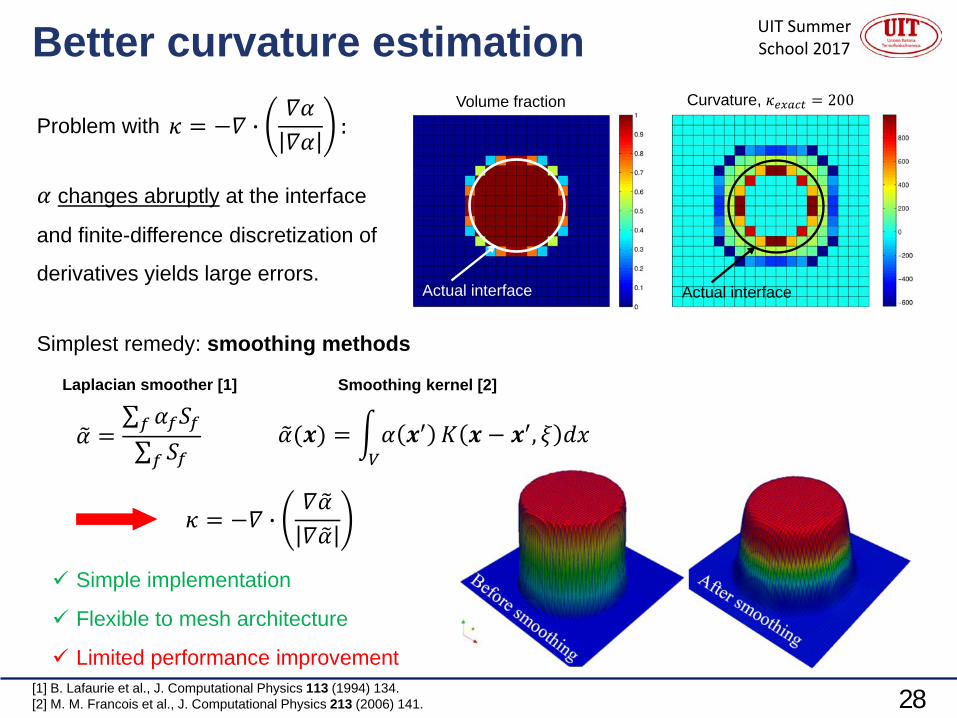
Better curvature estimation

Problem with

𝛼𝛼 changes abruptly at the interface

and finite-difference discretization of

derivatives yields large errors.

𝜎𝜎 = −𝛻𝛻 �𝛻𝛻𝛼𝛼𝛻𝛻𝛼𝛼

:

[1] B. Lafaurie et al., J. Computational Physics 113 (1994) 134.[2] M. M. Francois et al., J. Computational Physics 213 (2006) 141.

Simplest remedy: smoothing methods

�𝛼𝛼 =∑𝑓𝑓 𝛼𝛼𝑓𝑓𝑆𝑆𝑓𝑓∑𝑓𝑓 𝑆𝑆𝑓𝑓

�𝛼𝛼(𝒙𝒙) = �𝑉𝑉𝛼𝛼 𝒙𝒙′ 𝐾𝐾 𝒙𝒙 − 𝒙𝒙′, 𝜉𝜉 𝑑𝑑𝑥𝑥

𝜎𝜎 = −𝛻𝛻 �𝛻𝛻 �𝛼𝛼𝛻𝛻 �𝛼𝛼

Simple implementation

Flexible to mesh architecture

Limited performance improvement

Laplacian smoother [1] Smoothing kernel [2]

Actual interface Actual interface

Volume fraction Curvature, 𝜎𝜎𝑖𝑖𝑥𝑥𝑠𝑠𝑐𝑐𝑠𝑠 = 200


29

The Height Function methodIt reconstructs a continuous field of

local interface heights 𝑑𝑑(𝑥𝑥), from

which 𝜎𝜎 is accurately computed [1,2].

On a continuous domain:

On a discretized domain:

Interface topology (2D):

[1] S. J. Cummins et al., Computers & Structures 83 (2005) 425.[2] M. Magnini, AMS Unibo Tesi Dottorato (2012).

𝑑𝑑 𝑥𝑥;𝑡 =1𝑡

�𝑥𝑥−ℎ/2

𝑥𝑥+ℎ/2

𝑜𝑜 𝑡𝑡 𝑑𝑑𝑡𝑡

𝑑𝑑𝑗𝑗 =1𝑡

�𝑠𝑠=−𝑠𝑠𝑙𝑙𝑙𝑙𝑙𝑙

𝑠𝑠𝑢𝑢𝑢𝑢

𝛼𝛼𝑖𝑖−𝑠𝑠,𝑗𝑗𝑡2

𝒏𝒏 =1

1 + 𝑑𝑑𝑥𝑥2 1/2 −𝑑𝑑𝑥𝑥 , 1 , 𝜎𝜎 =𝑑𝑑𝑥𝑥𝑥𝑥

1 + 𝑑𝑑𝑥𝑥2 3/2

2nd order accurate curvatures

Not flexible to mesh architecture

It fails badly if the mesh is too coarse

Actual interface Actual interface

Volume fraction Curvature, 𝜎𝜎𝑖𝑖𝑥𝑥𝑠𝑠𝑐𝑐𝑠𝑠 = 200


30

Algebraic coupling of LS and VOFA level set function 𝜙𝜙 is reconstructed (but not advected) from the volume fraction field and

the interface curvature is estimated using derivatives of 𝜙𝜙 as in the LS method.

flexCLV: flexible Coupled Ls and Vof [1] - 𝜙𝜙 is reconstructed as the distance from the 𝛼𝛼 = 0.5

interface line. A characteristic mesh size is identified for computing 𝛿𝛿𝑆𝑆 in any kind of mesh.

[1] A. Ferrari et al., Int. J. Multiphase Flow 91 (2017) 276.

Rising bubble testsHex mesh

Tet mesh

3D capillary flow in a tube


31

Validation benchmarksReconstruction of a circular interface [1,2]

Useful to test the calculation of 𝒏𝒏 and 𝜎𝜎.

gas

liquid

2R

L

𝐿𝐿2 𝒏𝒏 =∑𝑁𝑁 𝒏𝒏𝒊𝒊 − 𝒏𝒏𝒆𝒆𝒙𝒙𝒘𝒘𝒆𝒆𝒆𝒆 2

𝑁𝑁𝐿𝐿2 𝜎𝜎 =

1𝜎𝜎𝑖𝑖𝑥𝑥𝑠𝑠𝑐𝑐𝑠𝑠

∑𝑁𝑁 𝜎𝜎𝑖𝑖 − 𝜎𝜎𝑖𝑖𝑥𝑥𝑠𝑠𝑐𝑐𝑠𝑠 2

𝑁𝑁

1st order

Mesh refinement Mesh refinement

2nd order

Divergence

Youngs: 𝒏𝒏 =𝛻𝛻𝛼𝛼𝛻𝛻𝛼𝛼

, 𝜎𝜎 = −𝛻𝛻 �𝛻𝛻𝛼𝛼𝛻𝛻𝛼𝛼 𝒏𝒏 =

𝛻𝛻 �𝛼𝛼𝛻𝛻 �𝛼𝛼

, 𝜎𝜎 = −𝛻𝛻 �𝛻𝛻 �𝛼𝛼𝛻𝛻 �𝛼𝛼Smoother:

𝒏𝒏 =1

1 + 𝑑𝑑𝑥𝑥2 1/2 −𝑑𝑑𝑥𝑥, 1

𝜎𝜎 =𝑑𝑑𝑥𝑥𝑥𝑥

1 + 𝑑𝑑𝑥𝑥2 3/2

HF:

[1] M. Magnini, AMS Unibo Tesi Dottorato (2012).[2] M. Magnini et al., Int. J. Heat Mass Transfer 59 (2013) 451.


32

Spurious velocity test2D inviscid static droplet - R=5 mm, R/h=10, ρ1=ρ2=1 kg/m3, σ=1 N/m

HF - Umax=7.26 mm/s Youngs - Umax=5.35 m/s


33

Experimental benchmarksRising bubble in an infinite pool of liquid:

Bhaga and Weber [1]

See [2] for higher surface tension cases

Bubbles in confined capillary flows

Khodaparast et al. [3]

[3] S. Khodaparast et al., Microfluid Nanofluid 19 (2015) 209.[1] D. Bhaga and M. E. Weber, J. Fluid Mechanics 105 (1981) 61.[2] G. Bozzano and M. Dente, Comput. Chem. Eng. 25 (2001) 571.


34

VOF: Phase changeMost popular modelling strategies

1) Approach based on thermal equilibrium at the

interface: 𝑇𝑇𝑠𝑠𝑠𝑠𝑠𝑠 𝑝𝑝𝑙𝑙 = 𝑇𝑇𝑙𝑙 ≅ 𝑇𝑇𝑣𝑣 = 𝑇𝑇𝑠𝑠𝑠𝑠𝑠𝑠 𝑝𝑝𝑣𝑣

𝑝𝑝𝑙𝑙 = 𝑝𝑝∞ 𝑝𝑝𝑣𝑣 = 𝑝𝑝𝑙𝑙 + 𝜎𝜎𝜎𝜎

liquid vapor

𝑣𝑣𝑖𝑖′′

𝑇𝑇𝑖𝑖

𝑇𝑇𝑙𝑙 𝑇𝑇𝑣𝑣

Schematic of interface conditions

In principle:

𝑇𝑇𝑖𝑖 = 𝑇𝑇𝑠𝑠𝑠𝑠𝑠𝑠 𝑝𝑝∞ is representative

of macroscale conditions.

𝑇𝑇𝑖𝑖 ≠ 𝑇𝑇𝑠𝑠𝑠𝑠𝑠𝑠 is representative of

microscale conditions.

𝑣𝑣𝑖𝑖′′ =

1𝑡𝑙𝑙𝑣𝑣

𝒒𝒒𝒘𝒘′′ − 𝒒𝒒𝒗𝒗′′ � 𝒏𝒏

2) Approach based on thermal equilibrium at the

interface according to Lee’s [1] model:

𝑣𝑣𝑖𝑖′′ 𝛻𝛻𝛼𝛼 = 𝑎𝑎 1 − 𝛼𝛼 𝜌𝜌𝑙𝑙

𝑇𝑇𝑖𝑖 − 𝑇𝑇𝑠𝑠𝑠𝑠𝑠𝑠𝑇𝑇𝑠𝑠𝑠𝑠𝑠𝑠

3) Approach based on departure from thermal

equilibrium at the interface: 𝑇𝑇𝑠𝑠𝑠𝑠𝑠𝑠 𝑝𝑝𝑙𝑙 = 𝑇𝑇𝑙𝑙 ≠ 𝑇𝑇𝑣𝑣 = 𝑇𝑇𝑠𝑠𝑠𝑠𝑠𝑠 𝑝𝑝𝑣𝑣


𝑡𝑖𝑖𝑡𝑙𝑙𝑣𝑣

𝑇𝑇𝑖𝑖 − 𝑇𝑇𝑠𝑠𝑠𝑠𝑠𝑠 𝑝𝑝𝑣𝑣

[1] W. H. Lee, A pressure iteration scheme for two-phase flow modeling, Tech. report, Los Alamos Lab. (1980).


35

1) Approach based on thermal equilibrium

It is based on the temperature boundary condition at the

interface 𝑇𝑇𝑖𝑖 = 𝑇𝑇𝑠𝑠𝑠𝑠𝑠𝑠 𝑝𝑝∞ .

Mass transfer rate from energy balance at interface [1]:

where:

PLIC reconstruction of interface

𝑇𝑇𝑙𝑙𝑝𝑝𝑙𝑙 = 𝑝𝑝∞

𝑇𝑇𝑣𝑣𝑝𝑝𝑣𝑣 ≅ 𝑝𝑝𝑙𝑙

liquid vapor

𝑇𝑇𝑖𝑖 = 𝑇𝑇𝑙𝑙 = 𝑇𝑇𝑣𝑣 = 𝑇𝑇𝑠𝑠𝑠𝑠𝑠𝑠




𝒒𝒒𝒘𝒘′′ − 𝒒𝒒𝒗𝒗′′ � 𝒏𝒏 =1𝑡𝑙𝑙𝑣𝑣

−𝑘𝑘𝑙𝑙𝜕𝜕𝑇𝑇𝜕𝜕𝑖𝑖 𝑖𝑖,𝑙𝑙

+ 𝑘𝑘𝑣𝑣𝜕𝜕𝑇𝑇𝜕𝜕𝑖𝑖 𝑖𝑖,𝑣𝑣

Temperature gradients have to be evaluated at the

interface, within each phase

this is the most difficult numerical task

𝜕𝜕𝑇𝑇𝜕𝜕𝑖𝑖 𝑖𝑖,𝑙𝑙

,𝜕𝜕𝑇𝑇𝜕𝜕𝑖𝑖 𝑖𝑖,𝑣𝑣

Temperature gradients at the liquid (i,l) and vapor side (i,v) of the interface

[1] A. Esmaeeli and G. Tryggvason, Int. J. Heat Mass Transfer 47 (2004) 5451.


36


[1] A. Mukherjee and S. Kandlikar, Microfluid Nanofluid 1 (2005) 137.

Most simplified numerical technique: a smooth heat flux

variation across the interface is assumed [1]:

where 𝛻𝛻𝑇𝑇 is computed across the interface region, and

the mixture fluid thermal conductivity is considered.

Inaccuracy: temperature profile typically has a kink at

the interface, and therefore 𝛻𝛻𝑇𝑇 is not well defined.

However, it is probably the most utilized method in the

CFD practice.

PLIC reconstruction

Temperature profile across the interface

𝒒𝒒𝒘𝒘′′ − 𝒒𝒒𝒗𝒗′′ ≈ 𝑘𝑘𝛻𝛻𝑇𝑇, 𝑘𝑘 = 𝑘𝑘𝑙𝑙 + 𝑘𝑘𝑣𝑣 − 𝑘𝑘𝑙𝑙 𝛼𝛼


𝑘𝑘𝛻𝛻𝑇𝑇 � 𝒏𝒏𝑡𝑙𝑙𝑣𝑣

𝒏𝒏 =𝛻𝛻𝛼𝛼𝛻𝛻𝛼𝛼


37


More accurate numerical technique: evaluation of

temperature gradients within each phase [1-4].

For the generic interface cell, 0<α<1:

1. Find the interface segment (PLIC) and 𝒙𝒙𝑖𝑖

2. Find 𝒏𝒏, for instance 𝒏𝒏 = ⁄𝛻𝛻𝛼𝛼 𝛻𝛻𝛼𝛼

3. Find 𝒙𝒙𝒘𝒘 = 𝒙𝒙𝒊𝒊 + ∆ � 𝒏𝒏, 𝒙𝒙𝒗𝒗 = 𝒙𝒙𝒊𝒊 − ∆ � 𝒏𝒏

4. Calculate 𝑇𝑇𝑙𝑙 = 𝑇𝑇 𝒙𝒙𝒘𝒘 and 𝑇𝑇𝑣𝑣 = 𝑇𝑇 𝒙𝒙𝒗𝒗 by

interpolation of neighbor cells values

5. Calculate gradients:

Temperature profile across the interface

Evaluation of gradients within each phase



−𝑘𝑘𝑙𝑙𝜕𝜕𝑇𝑇𝜕𝜕𝑖𝑖 𝑖𝑖,𝑙𝑙

+ 𝑘𝑘𝑣𝑣𝜕𝜕𝑇𝑇𝜕𝜕𝑖𝑖 𝑖𝑖,𝑣𝑣

𝜕𝜕𝑇𝑇𝜕𝜕𝑖𝑖 𝑖𝑖,𝑙𝑙

=𝑇𝑇𝑠𝑠𝑠𝑠𝑠𝑠 − 𝑇𝑇𝑙𝑙𝒙𝒙𝒘𝒘 − 𝒙𝒙𝒊𝒊

=𝑇𝑇𝑠𝑠𝑠𝑠𝑠𝑠 − 𝑇𝑇𝑙𝑙

∆,𝜕𝜕𝑇𝑇𝜕𝜕𝑖𝑖 𝑖𝑖,𝑣𝑣

=𝑇𝑇𝑣𝑣 − 𝑇𝑇𝑠𝑠𝑠𝑠𝑠𝑠𝒙𝒙𝑣𝑣 − 𝒙𝒙𝒊𝒊

=𝑇𝑇𝑣𝑣 − 𝑇𝑇𝑠𝑠𝑠𝑠𝑠𝑠

∆[1] A. Esmaeeli and G. Tryggvason, Int. J. Heat Mass Transfer 47 (2004) 5451.[2] H.S. Udaykumar et al., Int. J. Numerical Methods in Fluids 22 (1996) 691.

[3] S.W.J. Welch and J. Wilson, J. Comp. Physics 160 (2000) 662.[4] C. Kunkelmann, PhD Thesis, TU Darmstadt (2011).

𝑇𝑇𝑠𝑠𝑠𝑠𝑠𝑠


38


Evaluation of gradients within each phase

[1] C. Kunkelmann, PhD Thesis, TU Darmstadt (2011).

𝑡 ≤ ∆≤ 2𝑡 such that 𝒙𝒙𝒘𝒘 and 𝒙𝒙𝒗𝒗 are outside the interfacial

region, where temperatures depend on the numerical

procedure used to estimate the mixture fluid properties.

Possible simplification: if 𝑞𝑞𝑣𝑣′′ ≪ 𝑞𝑞𝑙𝑙′′ (𝑘𝑘𝑣𝑣 ≪ 𝑘𝑘𝑙𝑙)

This procedure is applicable only to interface cells, 0<α<1.

However, 𝑣𝑣𝑖𝑖′′ must be defined in all the cells where 𝛿𝛿𝑠𝑠 =

𝛻𝛻𝛼𝛼 ≠ 0.

One possible remedy is to send the gradients data to the

neighbor cells where 𝛼𝛼 is either 0 or 1 [1]. Schematic of gradients transfer


1𝑡𝑙𝑙𝑣𝑣∆

𝑘𝑘𝑙𝑙 𝑇𝑇𝑙𝑙 − 𝑇𝑇𝑠𝑠𝑠𝑠𝑠𝑠 − 𝑘𝑘𝑣𝑣 𝑇𝑇𝑠𝑠𝑠𝑠𝑠𝑠 − 𝑇𝑇𝑣𝑣


𝑘𝑘𝑙𝑙 𝑇𝑇𝑙𝑙 − 𝑇𝑇𝑠𝑠𝑠𝑠𝑠𝑠𝑡𝑙𝑙𝑣𝑣∆


39

2) Approach based on thermal eq., Lee’s model

It is based on the temperature boundary condition at the

interface 𝑇𝑇𝑖𝑖 = 𝑇𝑇𝑠𝑠𝑠𝑠𝑠𝑠 𝑝𝑝∞ .

The model derives from Lee [1] and was first used in CFD

by Yang et al. [2].

where Ti is the local cell temperature and r [1/s] is a case-dependent empirical coefficient

which is also function of the mesh size.

Very different values of r have been used in the CFD practice:

• Lee [1]: r=0.1 1/s

• Yang et al. [2]: r~100 1/s

• Da Riva and Del Col [3]: r~106 1/s

𝑇𝑇𝑙𝑙𝑝𝑝𝑙𝑙 = 𝑝𝑝∞

𝑇𝑇𝑣𝑣𝑝𝑝𝑣𝑣 ≅ 𝑝𝑝𝑙𝑙

liquid vapor

𝑇𝑇𝑖𝑖 = 𝑇𝑇𝑙𝑙 = 𝑇𝑇𝑣𝑣 = 𝑇𝑇𝑠𝑠𝑠𝑠𝑠𝑠


[1] W. H. Lee, Tech. report, Los Alamos Lab. (1980).[2] Z. Yang et al., Int. J. Heat Mass Transfer 51 (2008) 1003.

𝑣𝑣𝑖𝑖′′ 𝛻𝛻𝛼𝛼 = �𝑎𝑎 1 − 𝛼𝛼 𝜌𝜌𝑙𝑙

𝑇𝑇𝑖𝑖 − 𝑇𝑇𝑠𝑠𝑠𝑠𝑠𝑠𝑇𝑇𝑠𝑠𝑠𝑠𝑠𝑠

, 𝑖𝑖𝑜𝑜 𝛻𝛻𝛼𝛼 ≠ 0

0, 𝑖𝑖𝑜𝑜 𝛻𝛻𝛼𝛼 = 0

[3] E. Da Riva and D. Del Col, ASME J. Heat Transfer 134 (2012) 051019.


40

3) Departure from thermal equilibrium

𝑣𝑣: mass of one molecule, 𝑘𝑘𝐴𝐴: Boltzmann constant

Departure from thermal equilibrium at the interface

is assumed, 𝑇𝑇𝑙𝑙 ≠ 𝑇𝑇𝑣𝑣.

Kinetic theory of gases: given a box of vapor

containing n molecules at p and T, with no bulk

motion, the Maxwell velocity distribution [1]:

Mass fluxes at a liquid-vapor interface [1]

yields the fraction of molecules with Cartesian velocities u,v,w in the range [u,u+du], [v+dv],

[w+dw].

Be 𝑆𝑆𝑖𝑖∗ a boundary surface of the box, located immediately adjacent to the interface, the flux

of molecules through this surface is:

𝑑𝑑𝑖𝑖𝑢𝑢𝑣𝑣𝑢𝑢𝑖𝑖

=𝑣𝑣

2𝜋𝜋𝑘𝑘𝐴𝐴𝑇𝑇

32𝑎𝑎𝑥𝑥𝑝𝑝 −

𝑣𝑣2𝑘𝑘𝐴𝐴𝑇𝑇

𝑣𝑣2 + 𝑣𝑣2 + 𝑤𝑤2 𝑑𝑑𝑣𝑣 𝑑𝑑𝑣𝑣 𝑑𝑑𝑤𝑤

�𝑀𝑀: molecular weight, �𝑅𝑅: universal gas constant𝑗𝑗𝑛𝑛 =�𝑀𝑀

2𝜋𝜋 �𝑅𝑅

1/2 𝑝𝑝𝑣𝑣𝑇𝑇1/2



41

3) Departure from thermal equilibriumMass fluxes at a liquid-vapor interface [1]

[1] V. P. Carey, Liquid-Vapor Phase Change Phenomena (1992).[2] R.W. Schrage, A theoretical study of interphase mass transfer, Columbia University Press, New York (1953).

Mass transfer rate: net difference between mass

flux of vapor molecules crossing 𝑆𝑆𝑖𝑖∗ towards the

interface, 𝑣𝑣𝑣𝑣′′, and those emerging from the liquid

side and crossing 𝑆𝑆𝑖𝑖∗ towards the bulk vapor, 𝑣𝑣𝑙𝑙′′,

>0: evaporation<0: condensation=0: no net phase change

𝑣𝑣𝑖𝑖′′ = 𝑣𝑣𝑙𝑙

′′ − 𝑣𝑣𝑣𝑣′′

Note that 𝑣𝑣𝑙𝑙′′ and 𝑣𝑣𝑣𝑣

′′ are always ≠0. Mass fluxes [2]:

𝛾𝛾𝑐𝑐: fraction of molecules that cross 𝑆𝑆𝑖𝑖∗ towards the interface and condense without being reflected.

𝑣𝑣𝑣𝑣′′ = 𝛾𝛾𝑐𝑐𝑣𝑣Γ𝑗𝑗𝑛𝑛,𝑣𝑣 = 𝛾𝛾𝑐𝑐Γ

�𝑀𝑀2𝜋𝜋 �𝑅𝑅

1/2 𝑝𝑝𝑣𝑣𝑇𝑇𝑣𝑣1/2

Correction function which accounts for the actual bulk motion of the vapor molecules within the vapor bulk phase.Γ = 1 +


𝑝𝑝𝑣𝑣𝜋𝜋 �𝑅𝑅𝑇𝑇𝑣𝑣2 �𝑀𝑀

1/2

𝛾𝛾𝑖𝑖: fraction of molecules that cross 𝑆𝑆𝑖𝑖∗ emerging from the liquid side and reach the bulk vapor phase.Bulk motion effects in liquid are neglected, i.e. Γ = 1.

𝑣𝑣𝑙𝑙′′ = 𝛾𝛾𝑖𝑖𝑣𝑣Γ𝑗𝑗𝑛𝑛,𝑙𝑙 = 𝛾𝛾𝑖𝑖


1/2 𝑝𝑝𝑙𝑙𝑇𝑇𝑙𝑙1/2


42

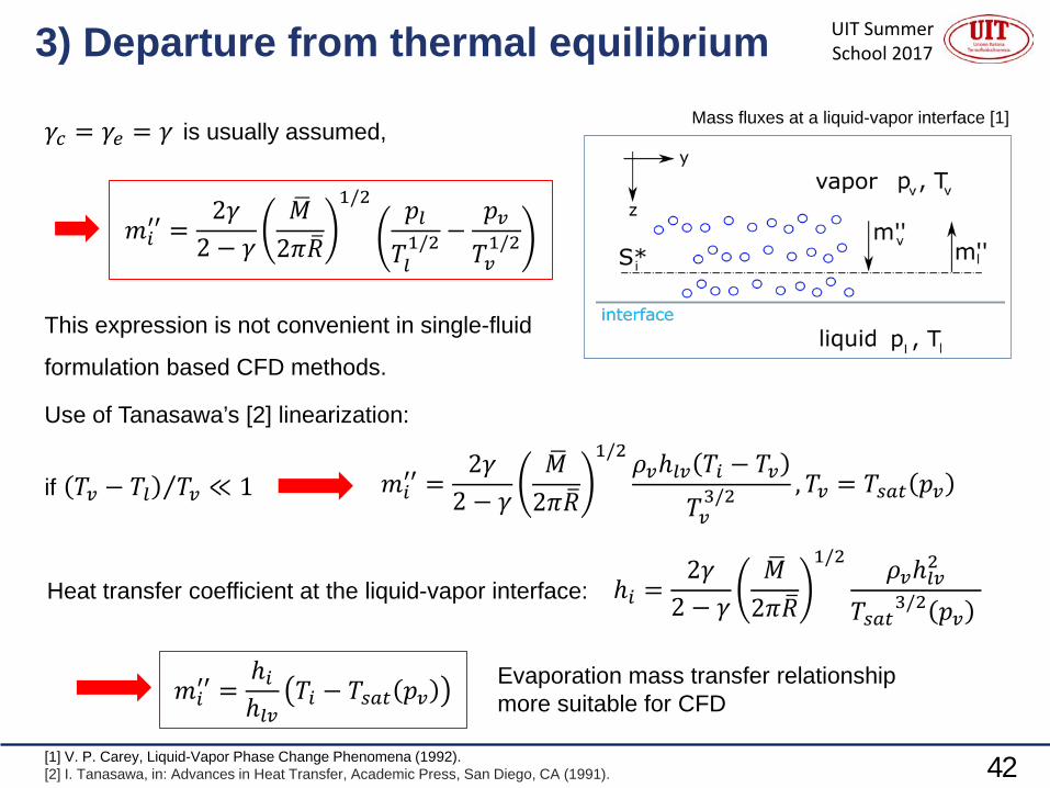
3) Departure from thermal equilibriumMass fluxes at a liquid-vapor interface [1]

[1] V. P. Carey, Liquid-Vapor Phase Change Phenomena (1992).[2] I. Tanasawa, in: Advances in Heat Transfer, Academic Press, San Diego, CA (1991).

𝛾𝛾𝑐𝑐 = 𝛾𝛾𝑖𝑖 = 𝛾𝛾 is usually assumed,


2𝛾𝛾2 − 𝛾𝛾


1/2 𝑝𝑝𝑙𝑙𝑇𝑇𝑙𝑙1/2 −

𝑝𝑝𝑣𝑣𝑇𝑇𝑣𝑣1/2

This expression is not convenient in single-fluid

formulation based CFD methods.

Use of Tanasawa’s [2] linearization:

if ⁄𝑇𝑇𝑣𝑣 − 𝑇𝑇𝑙𝑙 𝑇𝑇𝑣𝑣 ≪ 1 𝑣𝑣𝑖𝑖′′ =



1/2 𝜌𝜌𝑣𝑣𝑡𝑙𝑙𝑣𝑣 𝑇𝑇𝑖𝑖 − 𝑇𝑇𝑣𝑣𝑇𝑇𝑣𝑣3/2 ,𝑇𝑇𝑣𝑣 = 𝑇𝑇𝑠𝑠𝑠𝑠𝑠𝑠 𝑝𝑝𝑣𝑣

Heat transfer coefficient at the liquid-vapor interface: 𝑡𝑖𝑖 =2𝛾𝛾

2 − 𝛾𝛾�𝑀𝑀

2𝜋𝜋 �𝑅𝑅

1/2 𝜌𝜌𝑣𝑣𝑡𝑙𝑙𝑣𝑣2

𝑇𝑇𝑠𝑠𝑠𝑠𝑠𝑠3/2 𝑝𝑝𝑣𝑣

Evaporation mass transfer relationship more suitable for CFD𝑣𝑣𝑖𝑖

′′ =𝑡𝑖𝑖𝑡𝑙𝑙𝑣𝑣



43


[1] M. Magnini and J.R. Thome, J. Heat Transfer 138 (2016) 021502.[2] S. Hardt and F. Wondra, J. Computational Physics 227 (2008) 5871.

Numerical implementation

Ti is the temperature in interfacial cells, i.e. cells with

0<α<1. 𝑣𝑣𝑖𝑖′′ is promptly available for these cells.

In order to evaluate 𝑣𝑣𝑖𝑖′′ in neighbor cells, where α=0 or

1 but 𝛻𝛻𝛼𝛼 ≠ 0, Ti data are transferred from interface

cells to next-to-interface cells [1].

𝑇𝑇𝑠𝑠𝑠𝑠𝑠𝑠 𝑝𝑝𝑣𝑣 is the saturation temperature at the local vapor

pressure. If 𝜎𝜎𝜎𝜎 ≪ 𝑝𝑝∞, it can be assumed that

𝑇𝑇𝑠𝑠𝑠𝑠𝑠𝑠 𝑝𝑝𝑣𝑣 ≅ 𝑇𝑇𝑠𝑠𝑠𝑠𝑠𝑠 𝑝𝑝∞ [2],

Region where the interface temperatrure is defined

Interface temperature data transfer


𝑡𝑖𝑖𝑡𝑙𝑙𝑣𝑣





1/2 𝜌𝜌𝑣𝑣𝑡𝑙𝑙𝑣𝑣 𝑇𝑇𝑖𝑖 − 𝑇𝑇𝑠𝑠𝑠𝑠𝑠𝑠 𝑝𝑝∞𝑇𝑇𝑠𝑠𝑠𝑠𝑠𝑠3/2 𝑝𝑝∞


44


Evaporation/condensation

coefficient

It depends on the properties of

the fluid molecule, e.g. its polarity.

𝛾𝛾𝑐𝑐 , 𝛾𝛾𝑖𝑖 ∈ 0,1 , but there is large

uncertainty about their values, for

instance values in the range

10−3, 1 have been proposed for

water [1].

In absence of more precise data,

in the CFD practice this is usually

set as 1 [2-4].Experimental values for evaporation/condensation coefficient of water [1]

[1] I. Tanasawa, in: Advances in Heat Transfer, Academic Press (1991).[2] C. Kunkelmann, PhD Thesis, TU Darmstadt (2011).

[3] S. Hardt and F. Wondra, J. Computational Physics 227 (2008) 5871.[4] M. Magnini et al., Int. J. Heat Mass Transfer 59 (2013) 451.


Motion of a flat interface due to evaporation. Heat in

the vapor phase is transferred by conduction [1,2]:

45

Validation benchmarks – 1D Stefan problem

[1] S. Hardt and F. Wondra, J. Computational Physics 227 (2008) 5871.[2] S.W.J. Welch and J. Wilson, J. Computational Physics 160 (2000) 662.

𝛼𝛼𝑣𝑣 =𝜆𝜆𝑣𝑣

𝜌𝜌𝑣𝑣𝑖𝑖𝑝𝑝,𝑣𝑣

𝜕𝜕𝑇𝑇𝜕𝜕𝑡𝑡

= 𝛼𝛼𝑣𝑣𝜕𝜕2𝑇𝑇𝜕𝜕𝑥𝑥2

, 0 < 𝑥𝑥 < 𝑥𝑥𝑖𝑖(𝑡𝑡)

boundary conditions𝑇𝑇 𝑥𝑥 = 0, 𝑡𝑡 = 𝑇𝑇𝑢𝑢𝑇𝑇 𝑥𝑥 = 𝑥𝑥𝑖𝑖(𝑡𝑡) , 𝑡𝑡 = 𝑇𝑇𝑠𝑠𝑠𝑠𝑠𝑠

initial condition𝑥𝑥𝑖𝑖(𝑡𝑡 = 0) = 0

interface energy jump condition𝜌𝜌𝑣𝑣𝑡𝑙𝑙𝑣𝑣𝑣𝑣𝑖𝑖 = −𝜆𝜆𝑣𝑣 �

𝜕𝜕𝑇𝑇𝜕𝜕𝑥𝑥 𝑥𝑥=𝑥𝑥𝑖𝑖(𝑠𝑠)

with β from: 𝛽𝛽exp 𝛽𝛽2 erf 𝛽𝛽 =𝑖𝑖𝑝𝑝,𝑣𝑣 𝑇𝑇𝑢𝑢 − 𝑇𝑇𝑠𝑠𝑠𝑠𝑠𝑠

𝜋𝜋𝑡𝑙𝑙𝑣𝑣

𝑥𝑥𝑖𝑖(𝑡𝑡) = 2𝛽𝛽 𝛼𝛼𝑣𝑣𝑡𝑡

𝑇𝑇 𝑥𝑥, 𝑡𝑡 = 𝑇𝑇𝑢𝑢 +𝑇𝑇𝑠𝑠𝑠𝑠𝑠𝑠 − 𝑇𝑇𝑢𝑢

erf 𝛽𝛽erf

𝑥𝑥2 𝛼𝛼𝑣𝑣𝑡𝑡


46

1D sucking interfaceMotion of a flat interface due to evaporation.

Heat transfer in the liquid phase is governed by

mixed conduction and convection [1,2]:

Sucking interface case, from Welch and Wilson [1]

xi(t) and T(x,t) are obtained by numerical solution of a 2nd order ODE

𝜉𝜉 = 𝑥𝑥 − �0

𝑠𝑠

𝑣𝑣𝑖𝑖 𝑡𝑡 𝑑𝑑𝑡𝑡


+ 𝑣𝑣𝑙𝑙 − 𝑣𝑣𝑖𝑖𝜕𝜕𝑇𝑇𝜕𝜕𝜉𝜉

= 𝛼𝛼𝑙𝑙𝜕𝜕2𝑇𝑇𝜕𝜕𝜉𝜉2

, 0 < 𝜉𝜉 < ∞

boundary conditions𝑇𝑇 𝜉𝜉 = 0, 𝑡𝑡 = 𝑇𝑇𝑠𝑠𝑠𝑠𝑠𝑠𝑇𝑇 𝜉𝜉 → ∞, 𝑡𝑡 = 𝑇𝑇∞

initial condition𝑇𝑇 𝜉𝜉, 𝑡𝑡 = 0 = 𝑇𝑇∞

normal velocity jump condition−𝜌𝜌𝑣𝑣𝑣𝑣𝑖𝑖 = 𝜌𝜌𝑙𝑙 𝑣𝑣𝑖𝑖 − 𝑣𝑣𝑙𝑙

energy jump condition𝜌𝜌𝑙𝑙 𝑣𝑣𝑙𝑙 − 𝑣𝑣𝑖𝑖 𝑡𝑙𝑙𝑣𝑣 = −𝜆𝜆𝑙𝑙 �𝜕𝜕𝑇𝑇𝜕𝜕𝜉𝜉 𝜉𝜉=0

[1] S.W.J. Welch and J. Wilson, J. Computational Physics 160 (2000) 662.[2] S. Hardt and F. Wondra, J. Computational Physics 227 (2008) 5871.


47

Vapor bubble growthA vapor bubble grows in an extensive pool of

uniformly superheated liquid, after homogeneous

nucleation. There exist two growth stages [1]:

• Inertia-controlled stage 𝑡𝑡 ↓𝑝𝑝𝑣𝑣 ≅ 𝑝𝑝𝑠𝑠𝑠𝑠𝑠𝑠 𝑇𝑇∞ ,𝑇𝑇𝑣𝑣 ≅ 𝑇𝑇∞

• Heat-transfer-controlled stage 𝑡𝑡 ↑𝑝𝑝𝑣𝑣 ≅ 𝑝𝑝∞,𝑇𝑇𝑣𝑣 ≅ 𝑇𝑇𝑠𝑠𝑠𝑠𝑠𝑠 𝑝𝑝∞

Heat transfer in the liquid region is governed by [1]:

Schematic of vapor bubble growth [1]𝑅𝑅 𝑡𝑡 =

23𝑇𝑇∞ − 𝑇𝑇𝑠𝑠𝑠𝑠𝑠𝑠 𝑝𝑝∞𝑇𝑇𝑠𝑠𝑠𝑠𝑠𝑠 𝑝𝑝∞

𝜌𝜌𝑣𝑣𝑡𝑙𝑙𝑣𝑣𝜌𝜌𝑙𝑙

1/2

𝑡𝑡


+ 𝑣𝑣𝜕𝜕𝑇𝑇𝜕𝜕𝑎𝑎

=𝛼𝛼𝑙𝑙𝑎𝑎2

𝜕𝜕𝜕𝜕𝑎𝑎

𝑎𝑎2𝜕𝜕𝑇𝑇𝜕𝜕𝑎𝑎

, 𝑅𝑅(𝑡𝑡) < 𝑎𝑎 < ∞

velocity in the liquid𝑣𝑣(𝑎𝑎, 𝑡𝑡) =𝑑𝑑𝑅𝑅𝑑𝑑𝑡𝑡

𝑅𝑅𝑎𝑎

2

Boundary conditions

𝑇𝑇 ∞, 𝑡𝑡 = 𝑇𝑇∞

𝑇𝑇 𝑅𝑅, 𝑡𝑡 = 𝑇𝑇𝑠𝑠𝑠𝑠𝑠𝑠 𝑝𝑝𝑣𝑣

Mass and energy conservation:

𝜌𝜌𝑣𝑣𝑡𝑙𝑙𝑣𝑣𝑑𝑑𝑅𝑅𝑑𝑑𝑡𝑡

= 𝜆𝜆𝑙𝑙 �𝜕𝜕𝑇𝑇𝜕𝜕𝑎𝑎 𝑟𝑟=𝑅𝑅(𝑠𝑠)

𝑇𝑇 𝑎𝑎, 𝑡𝑡 = 0 = 𝑇𝑇∞Initial condition



48

Vapor bubble growthAnalytical solution for heat-transfer-controlled growth stage [1,2]:

Numerical solution [2]

• 2D axisymmetrical

domain 0.8×0.4 mm

• Initial bubble radius

R0=0.1 mm

• Mesh size 1 µm

• CFD bubble growth rate:

Growth at different time instants

0.1 mm

axis

0.4

mm

0.8 mm

liquidp 8

TL=TSAT( )+5°Cp 8

vaporTV=TSAT( )p 8

thermalboundary layer

Simulation setup

Growth vs time

𝑅𝑅(𝑡𝑡) = 2𝛽𝛽 𝛼𝛼𝑙𝑙𝑡𝑡

𝛽𝛽 = 𝐽𝐽𝑎𝑎 3/𝜋𝜋 𝐽𝐽𝑎𝑎 =𝑇𝑇∞ − 𝑇𝑇𝑠𝑠𝑠𝑠𝑠𝑠 𝜌𝜌𝑙𝑙𝑖𝑖𝑝𝑝,𝑙𝑙

𝜌𝜌𝑣𝑣𝑡𝑙𝑙𝑣𝑣

𝑅𝑅(𝑡𝑡) =3𝑉𝑉𝑏𝑏(𝑡𝑡)

4𝜋𝜋

1/3

[1] C. Kunkelmann, PhD Thesis, TU Darmstadt (2011).[2] M. Magnini et al., Int. J. Heat Mass Transfer 59 (2013) 451.


49

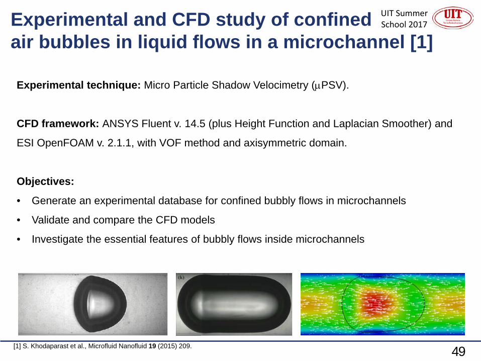
Experimental and CFD study of confined air bubbles in liquid flows in a microchannel [1]

Experimental technique: Micro Particle Shadow Velocimetry (µPSV).

CFD framework: ANSYS Fluent v. 14.5 (plus Height Function and Laplacian Smoother) and

ESI OpenFOAM v. 2.1.1, with VOF method and axisymmetric domain.

Objectives:

• Generate an experimental database for confined bubbly flows in microchannels

• Validate and compare the CFD models

• Investigate the essential features of bubbly flows inside microchannels

[1] S. Khodaparast et al., Microfluid Nanofluid 19 (2015) 209.


50

Experimental facility (µPSV)

Air-glycerol, d*<1, Ca=0.05, Re«1 Air-glycerol, d*>1, Ca=0.06, Re«1

Optical system:

Backlit illumination

Low power continuous LED

Bubble profile

Liquid flow field

Flow conditions:

d=0.5 mm

Fluids: air, water, glycerol

2.010Ca 4 −== −

σµ dcU

34 1010Re −== −

c

dc dUµ

ρ

5.21.0* −== ddd eq

Simultaneous detection


51

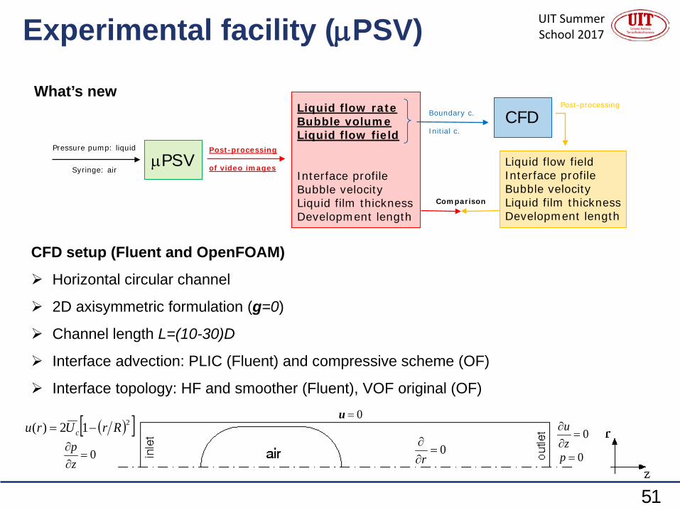
Experimental facility (µPSV)

CFD setup (Fluent and OpenFOAM)

Horizontal circular channel

2D axisymmetric formulation (g=0)

Channel length L=(10-30)D

Interface advection: PLIC (Fluent) and compressive scheme (OF)

Interface topology: HF and smoother (Fluent), VOF original (OF)0=u

( )[ ]212)( RrUru c −=

0=∂∂

zp 0=

∂∂r

0=∂∂

zu

0=p

Post-processing

of video images

CFD

µPSVPressure pump: liquid

Syringe: airLiquid flow fieldInterface profileBubble velocityLiquid film thicknessDevelopment length

Liquid flow rateBubble volumeLiquid flow field

Interface profileBubble velocityLiquid film thicknessDevelopment length

Boundary c.

Initial c.

Post-processing

Comparison

What’s new


52

Results

Blue: µPSV, red: ANSYS FluentAir-glycerol (Ca=0.01-0.2) Air-water (Ca=10-4-0.02)

Air-glycerol flow, Ca=0.05

Air-water flow, Ca=9·10-4

IncreasingC

a


53

Tips and tricks• Don’t blindly trust experimental results. Try to get most of the measurements from direct

processing of video images.

• Wetting the channel wall may require hours of preliminary liquid-only flow run at high

pressure.

• Controlling the flow rate or the pressure drop may yield different profiles of the tail of the

bubble in the experiments.

• If the objective is to compare experiments and simulations, try to set-up the facility in

order for the boundary conditions to be correctly reproduced by the numerics.

• Try to have always at least 7-10 mesh cells discretizing the liquid film zone.

• Someone said that you need square mesh cells to well capture the interface dynamics [1],

don’t believe it. Use wall-refined cells if you can.

• Careful with OpenFOAM-InterFOAM: errors in the curvature calculation become important

when Re>>1.

• Careful with OpenFOAM-InterFOAM: the default solver options fail when Re<<1, need to

disable the momentumPredictor step.

[1] R. Gupta et al., Chemical Engineering Science 65 (2010) 2094.


54

CFD study of slug flow boiling inmicrochannels [1-4]

CFD framework: ANSYS Fluent v. 14.5, with VOF-PLIC method and axisymmetric domain,

and self-developed UDF functions:

• Height Function

• Phase change (departure from thermal equilibrium)

• Vapor bubble generation

Objectives:

• Validate the CFD models

• Investigate local fluid dynamics and heat transfer mechanisms for single bubble, two-

bubble and multiple bubble flows

• Advance boiling heat transfer prediction methods

[1] M. Magnini et al., Int. J. Heat Mass Transfer 59 (2013) 451.[2] M. Magnini et al., Int. J. Thermal Sciences 71 (2013) 36.

[3] M. Magnini and J. R. Thome, Int. J. Thermal Sciences 110 (2016) 119.[4] M. Magnini and J. R. Thome, J. Heat Transfer 138 (2016) 021502.


55

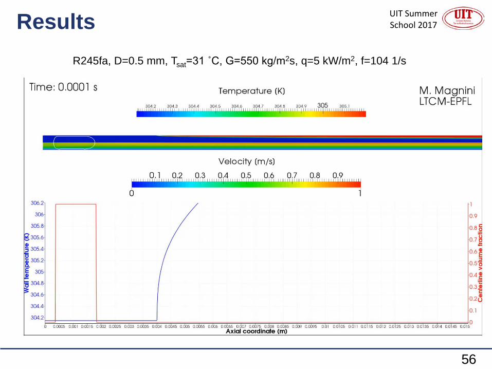
CFD setup t=0: liquid-only steady-state solution

Inlet condition: saturated liquid inflow

t>0: vapor bubbles generated with constant frequency

Simulations end when steady-periodic regime is achieved

Working conditions [1]

Channel size: D=0.3-0.7 mm

Fluid: R245fa

Saturation temperature: Tsat=10-50 °C

Heat flux: q=5-20 kW/m2

Mass flux G=400-700 kg/(m2s)

Bubble frequency: fbub=72-209 1/s

Initial temperature field

[1] L. Consolini and J. R. Thome, Microfluid Nanofluid 6 (2009) 731.


56

ResultsR245fa, D=0.5 mm, Tsat=31 ˚C, G=550 kg/m2s, q=5 kW/m2, f=104 1/s


57

A model for heat transfer

2 zones flow decomposition (no dryout)

Cylindrical bubbles

Thermal inertia of the liquid film

Transient dynamics of recirculating flows

( ),

)(1

1)(

1

02

δδ

λδλ

βα∑=

−−+= m

ii

tti

l

lfilm

Yecq

thit ( ) ( )sats

s

l

ss

ls

m

ii

tti

s

ls

lslug

TTqh

Yecq

thit −+++

=

∑=

−−

δλ

δλδ

δλδ

λβα )(1

1)(

1

02

Flow domain decomposition

CFD: h=2676 W/m2K

New model [1]: h=2630 W/m2K (-1.7%)

Three-zone model [2]: h=3604 W/m2K (+35%)

[1] M. Magnini and J. R. Thome, Int. J. Multiphase Flow 91 (2017) 296.[2] J. R. Thome et al., Int. J. Heat Mass Transfer 47 (2004) 3375.


58

Tips and tricks

• The velocity boundary condition always let the bubbles flow through the channel, while with

pressure conditions bubbles may get stuck when evaporate.

• Water is never a friendly fluid to be simulated in the slug flow boiling regime.

• When the bubbles leave the domain through the outflow boundary, they make a mess:

eliminate them as soon as their nose approaches the boundary.

• The phase change model based on the 3rd method is dramatically mesh dependent: you

need at least 10 mesh cells in the liquid film to get converged results.

• The bubble frequency has a huge impact on heat transfer and it is typically not known in

flow boiling experiments: comparison with experiments requires attention.

• Export data as text files while the simulation is running: a great deal of information can be

extracted and sytematically postprocessed with an external software (e.g. Matlab, Python).

• Take your time to find the most efficient solver options (mesh size, max Courant number,

residuals limit, max n. of iterations, etc.): it can save days of calculations afterwards.

• Trust your raw data, trust less your processed data.


59

Trapped water displacement in oil pipelinesExperimental technique: measurements of water withdrawal from the pipeline (Tel Aviv

University) [1,2]

CFD framework: ESI OpenFOAM v. 2.3.1, with VOF method and 3D domain. Additional

self-developed subroutine:

• Laplacian smoother for interface curvature calculation

Objectives:

• Study the fluid dynamics governing water displacement for different wetting conditions

• Identify flow conditions promoting water withdrawal

[1] G. Xu et al., Int. J. Multiphase Flow 37 (2011) 1.[2] G. Xu et al., J. Petroleum Science Engineering 147 (2016) 829.


60

CFD setup

Oil Water

ρ [kg/m3] 856 997

µ [mPa∙s] 3.43 0.895

σ [mN/m] 18.33

D [mm] 27

L [m] 0.027+1+0.5

θ [deg] 15−150

Uo [m/s] 0.05 − 0.25

Re 400 − 1600

Vw [ml] 5 − 115

Fluids properties

Flow conditions

Mesh study

Block-structured mesh (∆=0.1−1 mm)


61

ResultsWater dynamics at different wetting conditions


62

Tips and tricks

• When the interface advection is done using a compressive algorithm, higher compression

is needed if the flow is parallel to the interface.

• Compressive algorithms may lose mass: always double check.

• Capturing the wall adhesion requires a well-refined mesh at the wall.

• Careful at boundaries where backflow may exist: use the OpenFOAM’s inletOutlet

boundary condition.

• 3D studies are very expensive: sometimes limitations are a resource, they force you to use

your brain to overcome them.


63

Thank you for your attention

september 2017 numerical methods cfd simulations of two ... · calculation of the surface tension...

Documents