sequences of games: a tool for taming complexity in ...shoup.net/papers/games.pdf · sequences of...

Sequences of Games:

A Tool for Taming Complexity in Security Proofs∗

Victor Shoup†

January 18, 2006

Abstract

This paper is brief tutorial on a technique for structuring security proofs as sequencesgames.

1 Introduction

Security proofs in cryptography may sometimes be organized as sequences of games. Incertain circumstances, this can be a useful tool in taming the complexity of security proofsthat might otherwise become so messy, complicated, and subtle as to be nearly impossible toverify. This technique appears in the literature in various styles, and with various degrees ofrigor and formality. This paper is meant to serve as a brief tutorial on one particular “style”of employing this technique, which seems to achieve a reasonable level of mathematical rigorand clarity, while not getting bogged down with too much formalism or overly restrictiverules. We do not make any particular claims of originality — it is simply hoped that othersmight profit from some of the ideas discussed here in reasoning about security.

At the outset, it should be noted that this technique is certainly not applicable toall security proofs. Moreover, even when this technique is applicable, it is only a tool fororganizing a proof — the actual ideas for a cryptographic construction and security analysismust come from elsewhere.

1.1 The Basic Idea

Security for cryptograptic primitives is typically defined as an attack game played betweenan adversary and some benign entity, which we call the challenger. Both adversary andchallenger are probabilstic processes that communicate with each other, and so we canmodel the game as a probability space. Typically, the definition of security is tied to someparticular event S. Security means that for every “efficient” adversary, the probability thatevent S occurs is “very close to” some specified “target probabilty”: typically, either 0,1/2, or the probability of some event T in some other game in which the same adversary isinteracting with a different challenger.

∗First public version: Nov. 30, 2004†Computer Science Dept. NYU. [email protected]

1

In the formal definitions, there is a security parameter: an integer tending to infinity, andin the previous paragraph, “efficient” means time bounded by a polynomial in the securityparameter, and “very close to” means the difference is smaller than the inverse of anypolynomial in the security parameter, for sufficiently large values of the security parameter.The term of art is negligibly close to, and a quantity that is negliglibly close to zero is justcalled negligible. For simplicity, we shall for the most part avoid any further discussion ofthe security parameter, and it shall be assumed that all algorithms, adversaries, etc., takethis value as an implicit input.

Now, to prove security using the sequence-of-games approach, one prodceeds as follows.One constructs a sequence of games, Game 0, Game 1, . . . , Game n, where Game 0 is theoriginal attack game with respect to a given adversary and cryptographic primitive. Let S0

be the event S, and for i = 1, . . . , n, the construction defines an event Si in Game i, usuallyin a way naturally related to the definition of S. The proof shows that Pr[Si] is negligiblyclose to Pr[Si+1] for i = 0, . . . , n − 1, and that Pr[Sn] is equal (or negligibly close) to the“target probability.” From this, and the fact that n is a constant, it follows that Pr[S] isnegligibly close to the “target probability,” and security is proved.

That is the general framework of such a proof. However, in constructing such proofs,it is desirable that the changes between succesive games are very small, so that analyzingthe change is as simple as possible. From experience, it seems that transitions betweensuccessive games can be restricted to one of three types:

Transitions based on indistinguishability. In such a transition, a small change is madethat, if detected by the adversary, would imply an efficient method of distinguishing be-tween two distributions that are indistinguishable (either statistically or computationally).For example, suppose P1 and P2 are assumed to be computationally indistinguishable dis-tributions. To prove that |Pr[Si] − Pr[Si+1]| is negligible, one argues that there exists adistinguishing algorithmD that “interpolates” between Game i and Game i+1, so that whengiven an element drawn from distribution P1 as input, D outputs 1 with probability Pr[Si],and when given an element drawn from distribution P2 as input, D outputs 1 with prob-abilty Pr[Si+1]. The indistinguishability assumption then implies that |Pr[Si] − Pr[Si+1]|is negligible. Usually, the construction of D is obvious, provided the changes made in thetransition are minimal. Typically, one designs the two games so that they could easilybe rewritten as a single “hybrid” game that takes an auxilliary input — if the auxiallaryinput is drawn from P1, you get Game i, and if drawn from P2, you get Game i + 1. Thedistinguisher then simply runs this single hybrid game with its input, and outputs 1 if theappropriate event occurs.

Transitions based on failure events. In such a transition, one argues that Games iand i + 1 proceed identically unless a certain “failure event” F occurs. To make this typeof argument as cleanly as possible, it is best if the two games are defined on the sameunderlying probability space — the only differences between the two games are the rulesfor computing certain random variables. When done this way, saying that the two gamesproceed identically unless F occurs is equivalent to saying that

Si ∧ ¬F ⇐⇒ Si+1 ∧ ¬F,

that is, the events Si ∧¬F and Si+1 ∧¬F are the same. If this is true, then we can use the

2

following fact, which is completely trivial, yet is so often used in these types of proofs thatit deserves a name:

Lemma 1 (Difference Lemma). Let A,B, F be events defined in some probability dis-tribution, and suppose that A ∧ ¬F ⇐⇒ B ∧ ¬F . Then |Pr[A]− Pr[B]| ≤ Pr[F ].

Proof. This is a simple calculation. We have

|Pr[A]− Pr[B]| = |Pr[A ∧ F ] + Pr[A ∧ ¬F ]− Pr[B ∧ F ]− Pr[B ∧ ¬F ]|= |Pr[A ∧ F ]− Pr[B ∧ F ]|≤ Pr[F ].

The second equality follows from the assumption that A ∧ ¬F ⇐⇒ B ∧ ¬F , and so inparticular, Pr[A ∧ ¬F ] = Pr[B ∧ ¬F ]. The final inequality follows from the fact that bothPr[A ∧ F ] and Pr[B ∧ F ] are numbers between 0 and Pr[F ]. 2

So to prove that Pr[Si] is negligibly close to Pr[Si+1], it suffices to prove that Pr[F ] isnegligible. Sometimes, this is done using a security assumption (i.e., when F occurs, theadversary has found a collision in a hash function, or forged a MAC), while at other times,it can be done using a purely information-theoretic argument.

Usually, the event F is defined and analyzed in terms of the random variables of oneof the two adjacent games. The choice is arbitrary, but typically, one of the games will bemore suitable than the other in terms of allowing a clear proof.

In some particularly challenging circumstances, it may be difficult to analyze the eventF in either game. In fact, the analysis of F may require its own sequence of games sproutingoff in a different direction, or the sequence of games for F may coincide with the sequence ofgames for S, so that Pr[F ] finally gets pinned down in Game j for j > i+1. This techniqueis sometimes crucial in side-stepping potential circularities.

Bridging steps. The third type of transition introduces a bridging step, which is typicallya way of restating how certain quantities can be computed in a completely equivalent way.The change is purely conceptual, and Pr[Si] = Pr[Si+1]. The reason for doing this is toprepare the ground for a transition of one of the above two types. While in principle, such abridging step may seem unnecessary, without it, the proof would be much harder to follow.

As mentioned above, in a transition based on a failure event, it is best if the twosuccessive games are understood to be defined on the same underlying probability space.This is an important point, which we repeat here for emphasis — it seems that proofsare easiest to understand if one does not need to compare “corresponding” events acrossdistinct and (by design) quite different probability spaces. Actually, it is good practiceto simply have all the games in the sequence defined on the same underlying probabilityspace. However, the Difference Lemma generalizes in the obvious way as follows: if A,B, F1 and F2 are events such that Pr[A ∧ ¬F1] = Pr[B ∧ ¬F2] and Pr[F1] = Pr[F2], then|Pr[A] − Pr[B]| ≤ Pr[F1]. With this generalized version, one may (if one wishes) analyzetransitions based on failure events when the underlying probability spaces are not the same.

3

1.2 Some Historical Remarks

“Hybrid arguments” have been used extensively in cryptography for many years. Such anargument is essentially a sequence of transitions based on indistinguishability. An earlyexample that clearly illustrates this technique is Goldreich, Goldwasser, and Micali’s paper[GGM86] on constructing pseudo-random functions (although this is by no means the ear-liest application of a hybrid argument). Note that in some applications, such as [GGM86],one in fact makes a non-constant number of transitions, which requires an additional, prob-abilistic argument.

Although some might use the term “hybrid argument” to include proofs that use transi-tions based on both indistinguishability and failure events, that seems to be somewhat of astretch of terminology. An early example of a proof that is clearly structured as a sequenceof games that involves transitions based on both indistinguishability and failure events isBellare and Goldwasser’s paper [BG89].

Kilian and Rogaway’s paper [KR96] on DESX initiates a somewhat more formal ap-proach to sequences of games. That paper essentially uses the Difference Lemma, specializedto their particular setting. Subsequently, Rogaway has refined and applied this technique innumerous works with several co-authors. We refer the reader to the paper [BR04] by Bellareand Rogaway that gives a detailed introduction to the methodology, as well as referencesto papers where it has been used. However, we comment briefly on some of the differencesbetween the technique discussed in this paper, and that advocated in [BR04]:

• In Bellare and Rogaway’s approach, games are programs and are treated as purelysyntactic objects subject to formal manipulation. In contrast, we view games asprobability spaces and random variables defined over them, and do not insist on anyparticular syntactic formalism beyond that convenient to make a rigorous mathemat-ical argument.

• In Bellare and Rogaway’s approach, transitions based on failure events are restrictedto events in which an executing program explicitly sets a particular boolean variableto true. In contrast, we do not suggest that events need to be explicitly “announced.”

• In Bellare and Rogaway’s approach, when the execution behaviors of two games arecompared, two distinct probability spaces are involved, and probabilities of “corre-sponding” events across probability spaces must be compared. In contrast, we sug-gest that games should be defined on a common probability space, so that whendiscussing, say, a particular failure event F , there is literally just one event, not a pairof corresponding events in two different probability spaces.

In the end, we think that the choice between the style advocated in [BR04] and thatsuggested here is mainly a matter of taste and convenience.

The author has used proofs organized as sequences of games extensively in his own work[Sho00, SS00, Sho01, Sho02, CS02, CS03b, CS03a, GS04] and has found them to be anindispensable tool — while some of the proofs in these papers could be structured differently,it is hard to imagine how most of them could be done in a more clear and convincing waywithout sequences of games (note that all but the first two papers above adhere to the rulesuggested here of defining games to operate on the same probability space). Other authors

4

have also been using very similar proof styles recently [AFP04, BK04, BCP02a, BCP02b,BCP03, CPP04, DF03, DFKY03, DFJW04, Den03, FOPS04, GaPMV03, KD04, PP03,SWP04]. Also, Pointcheval [Poi04] has a very nice introductory manuscript on public-keycryptography that illustrates this proof style on a number of particular examples.

The author has also been using the sequence-of-games technique extensively in teachingcourses in cryptography. Many “classical” results in cryptography can be fruitfully analyzedusing this technique. Generally speaking, it seems that the students enjoy this approach,and easily learn to use and apply it themselves. Also, by using a consistent framework foranalysis, as an instructor, one can more easily focus on the ideas that are unique to anyspecific application.

1.3 Outline of the Rest of the Paper

After recalling some fairly standard notation in the next section, the following sectionsillustrate the use of the sequence-of-games technique in the analysis of a number of classicalcryptographic constructions. Compared to many of the more technically involved examplesin the literature of this technique (mentioned above), the applications below are really just“toy” examples. Nevertheless, they serve to illustrate the technique in a concrete way, andmoreover, we believe that the proofs of these results are at least as easy to follow as any otherproof, if not more so. All of the examples, except the last two (in §§7-8), are presented at anextreme level of detail; indeed, for these examples, we give complete, detailed descriptionsof each and every game. More typically, to produce a more compact proof, one might simplydescribe the differences between games, rather than describing each game in its entirety (asis done in §§7-8). These examples are based mainly on lectures in courses on cryptographytaught by the author.

2 Notation

We make use of fairly standard notation in what follows.In describing probabilistic processes, we write

x c|← X

to denote the action of assigning to the variable x a value sampled according to the dis-tribution X. If S is a finite set, we simply write s c|← S to denote assignment to s of anelement sampled from the uniform distribution on S. If A is a probabilistic algorithm andx an input, then A(x) denotes the output distribution of A on input x. Thus, we writey c|← A(x) to denote the action of running algorithm A on input x and assigning the outputto the variable y.

We shall write

Pr[x1c|← X1, x2

c|← X2(x1), . . . , xnc|← Xn(x1, . . . , xn−1) : φ(x1, . . . , xn)]

to denote the probability that when x1 is drawn from a certain distribution X1, and x2 isdrawn from a certain distribution X2(x1), possibly depending on the particular choice of

5

x1, and so on, all the way to xn, the predicate φ(x1, . . . , xn) is true. We allow the predicateφ to involve the execution of probabilistic algorithms.

If X is a probability distribution on a sample space X , then [X] denotes the subset ofelements of X that occur with non-zero probability.

3 ElGamal Encryption

3.1 Basic Definitions

We first recall the basic definition of a public-key encryption scheme, and the notion ofsemantic security.

A public-key encryption scheme is a triple of probabilistic algorithms (KeyGen, E,D).The key generation algorithm KeyGen takes no input (other than an implied security pa-rameter, and perhaps other system parameters), and outputs a public-key/secret-key pair(pk , sk). The encryption algorithm E takes as input a public key pk and a message m,selected from a message space M , and outputs a ciphertext ψ. The decryption algorithmtakes as input a secret key sk and ciphertext ψ, and outputs a message m.

The basic correctness requirement is that decryption “undoes” encryption. That is, forall m ∈ M , all (pk , sk) ∈ [KeyGen()], all ψ ∈ [E(pk ,m)], and all m′ ∈ [D(sk , ψ)], we havem = m′. This definition can be relaxed in a number of ways; for example, we may onlyinsist that it is computationally infeasible to find a message for which decryption does not“undo” its encryption.

The notion of semantic security intuitively says that an adversary cannot effectively dis-tinguish between the encryption of two messages of his choosing (this definition comes from[GM84], where is called polynomial indistinguishability, and semantic security is actuallythe name of a syntactically different, but equivalent, characterization). This is formallydefined via a game between an adversary and a challenger.

• The challenger computes (pk , sk) c|← KeyGen(), and gives pk to the adversary.

• The adversary chooses two messages m0,m1 ∈M , and gives these to the challenger.

• The challenger computes

b c|← {0, 1}, ψ c|← E(pk ,mb)

and gives the “target ciphertext” ψ to the adversary.

• The adversary outputs b̂ ∈ {0, 1}.

We define the SS-advantage of the adversary to be |Pr[b = b̂] − 1/2|. Semantic securitymeans that any efficient adversary’s SS-advantage is negligible.

3.2 The ElGamal Encryption Scheme

We next recall ElGamal encryption. Let G be a group of prime order q, and let γ ∈ G bea generator (we view the descriptions of G and γ, including the value q, to be part of a setof implied system parameters).

6

The key generation algorithm computes (pk , sk) as follows:

x c|← Zq, α← γx, pk ← α, sk ← x.

The message space for the algorithm is G. To encrypt a message m ∈ G, the encryptionalgorithm computes a ciphertext ψ as follows:

y c|← Zq, β ← γy, δ ← αy, ζ ← δ ·m, ψ ← (β, ζ).

The decryption algorithm takes as input a ciphertext (β, ζ), and computes m as follows:

m← ζ/βx.

It is clear that decryption “undoes” encryption. Indeed, if β = γy and ζ = αy ·m, then

ζ/βx = αym/βx = (γx)ym/(γy)x = γxym/γxy = m.

3.3 Security Analysis

ElGamal encryption is semantically secure under the Decisional Diffie-Hellman (DDH)assumption. This is the assumption that it is hard to distinguish triples of the form(γx, γy, γxy) from triples of the form (γx, γy, γz), where x, y, and z are random elements ofZq.

The DDH assumption is more precisely formulated as follows. Let D be an algorithmthat takes as input triples of group elements, and outputs a bit. We define the DDH-advantage of D to be

|Pr[x, y c|← Zq : D(γx, γy, γxy) = 1]− Pr[x, y, z c|← Zq : D(γx, γy, γz) = 1]|.

The DDH assumption (for G) is the assumption that any efficient algorithm’s DDH-advantage is negligible.

We now give a proof of the semantic security of ElGamal encryption under the DDHassumption, using a sequence of games.

Game 0. Fix an efficient adversary A. Let us define Game 0 to be the attack game againstA in the definition of semantic security. To make things more precise and more concrete,we may describe the attack game algorithmically as follows:

x c|← Zq, α← γx

r c|← R, (m0,m1)← A(r, α)b c|← {0, 1}, y c|← Zq, β ← γy, δ ← αy, ζ ← δ ·mb

b̂← A(r, α, β, ζ)

In the above, we have modeled the adversary A is a deterministic algorithm that takesas input “random coins” r sampled uniformly from some set R. It should be evident thatthis algorithm faithfully represents the attack game. If we define S0 to be the event thatb = b̂, then the adversary’s SS-advantage is |Pr[S0]− 1/2|.

7

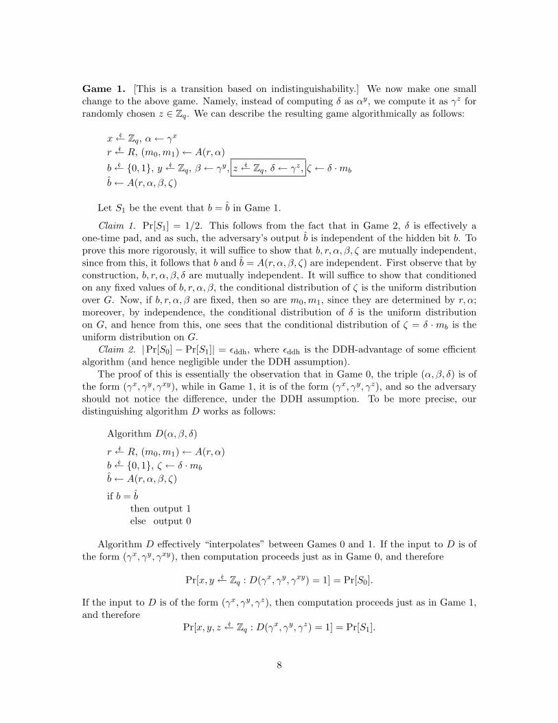
Game 1. [This is a transition based on indistinguishability.] We now make one smallchange to the above game. Namely, instead of computing δ as αy, we compute it as γz forrandomly chosen z ∈ Zq. We can describe the resulting game algorithmically as follows:


r c|← R, (m0,m1)← A(r, α)

b c|← {0, 1}, y c|← Zq, β ← γy, z c|← Zq, δ ← γz, ζ ← δ ·mb

b̂← A(r, α, β, ζ)

Let S1 be the event that b = b̂ in Game 1.

Claim 1. Pr[S1] = 1/2. This follows from the fact that in Game 2, δ is effectively aone-time pad, and as such, the adversary’s output b̂ is independent of the hidden bit b. Toprove this more rigorously, it will suffice to show that b, r, α, β, ζ are mutually independent,since from this, it follows that b and b̂ = A(r, α, β, ζ) are independent. First observe that byconstruction, b, r, α, β, δ are mutually independent. It will suffice to show that conditionedon any fixed values of b, r, α, β, the conditional distribution of ζ is the uniform distributionover G. Now, if b, r, α, β are fixed, then so are m0,m1, since they are determined by r, α;moreover, by independence, the conditional distribution of δ is the uniform distributionon G, and hence from this, one sees that the conditional distribution of ζ = δ ·mb is theuniform distribution on G.

Claim 2. |Pr[S0] − Pr[S1]| = εddh, where εddh is the DDH-advantage of some efficientalgorithm (and hence negligible under the DDH assumption).

The proof of this is essentially the observation that in Game 0, the triple (α, β, δ) is ofthe form (γx, γy, γxy), while in Game 1, it is of the form (γx, γy, γz), and so the adversaryshould not notice the difference, under the DDH assumption. To be more precise, ourdistinguishing algorithm D works as follows:

Algorithm D(α, β, δ)

r c|← R, (m0,m1)← A(r, α)b c|← {0, 1}, ζ ← δ ·mb

b̂← A(r, α, β, ζ)

if b = b̂then output 1else output 0

Algorithm D effectively “interpolates” between Games 0 and 1. If the input to D is ofthe form (γx, γy, γxy), then computation proceeds just as in Game 0, and therefore

Pr[x, y c|← Zq : D(γx, γy, γxy) = 1] = Pr[S0].

If the input to D is of the form (γx, γy, γz), then computation proceeds just as in Game 1,and therefore

Pr[x, y, z c|← Zq : D(γx, γy, γz) = 1] = Pr[S1].

8

From this, it follows that the DDH-advantage of D is equal to |Pr[S0] − Pr[S1]|. Thatcompletes the proof of Claim 2.

Combining Claim 1 and Claim 2, we see that

|Pr[S0]− 1/2| = εddh,

and this is negligible. That completes the proof of security of ElGamal encryption.

3.4 Hashed ElGamal

For a number of reasons, it is convenient to work with messages that are bit strings, say, oflength `, rather than group elements. Because of this, one may choose to use a “hashed”version of the ElGamal encryption scheme.

This scheme makes use of a family of keyed “hash” functions H := {Hk}k∈K , whereeach Hk is a function mapping G to {0, 1}`.

The key generation algorithm computes (pk , sk) as follows:

x c|← Zq, kc|← K, α← γx, pk ← (α, k), sk ← (x, k).

To encrypt a message m ∈ {0, 1}`, the encryption algorithm computes a ciphertext ψas follows:

y c|← Zq, β ← γy, δ ← αy, h← Hk(δ), v ← h⊕m, ψ ← (β, v).

The decryption algorithm takes as input a ciphertext (β, v), and computes m as follows:

m← Hk(βx)⊕ v.

The reader may easily verify that decryption “undoes” encryption.As for semantic security, this can be proven under the DDH assumption and the as-

sumption that the family of hash functions H is “entropy smoothing.” Loosely speaking,this means that it is hard to distinguish (k,Hk(δ)) from (k, h), where k is a random elementof K, δ is a random element of G, and h is a random element of {0, 1}`. More formally,let D be an algorithm that takes as input an element of K and an element of {0, 1}`, andoutputs a bit. We define the ES-advantage of D to be

|Pr[k c|← K, δ c|← G : D(k,Hk(δ)) = 1]− Pr[k c|← K, h c|← {0, 1}` : D(k, h) = 1]|.

We say H is entropy smoothing if every efficient algorithm’s ES-advantage is negligible.It is in fact possible to construct entropy smoothing hash function families without ad-

ditional hypothesis (the Leftover Hash Lemma may be used for this [IZ89]). However, thesemay be somewhat less practical than ad hoc hash function families for which the entropysmoothing property is only a (perfectly reasonable) conjecture; moreover, our definition alsoallows entropy smoothers that use pseudo-random bit generation techniques as well.

We now sketch the proof of semantic security of hashed ElGamal encryption, under theDDH assumption and the assumption that H is entropy smoothing.

9

Game 0. This is the original attack game, which we can state algorithmically as follows:

x c|← Zq, kc|← K, α← γx

r c|← R, (m0,m1)← A(r, α, k)b c|← {0, 1}, y c|← Zq, β ← γy, δ ← αy, h← Hk(δ), v ← h⊕mb

b̂← A(r, α, k, β, v)

We define S0 to be the event that b = b̂ in Game 0.

Game 1. [This is a transition based on indistinguishability.] Now we transform Game 0into Game 1, computing δ as γz for random z ∈ Zq. We can state Game 1 algorithmicallyas follows:


r c|← R, (m0,m1)← A(r, α, k)

b c|← {0, 1}, y c|← Zq, β ← γy, z c|← Zq, δ ← γz, h← Hk(δ), v ← h⊕mb

b̂← A(r, α, k, β, v)

Let S1 be the event that b = b̂ in Game 1. We claim that

|Pr[S0]− Pr[S1]| = εddh, (1)

where εddh is the DDH-advantage of some efficient algorithm (which is negligible under theDDH assumption).

The proof of this is almost identical to the proof of the corresponding claim for “plain”ElGamal. Indeed, the following algorithm D “interpolates” between Game 0 and Game 1,and so has DDH-advantage equal to |Pr[S0]− Pr[S1]|:

Algorithm D(α, β, δ)

k c|← K

r c|← R, (m0,m1)← A(r, α, k)b c|← {0, 1}, h← Hk(δ), v ← h⊕mb

b̂← A(r, α, k, β, v)


Game 2. [This is also a transition based on indistinguishability.] We now transformGame 1 into Game 2, computing h by simply choosing it at random, rather than as a hash.Algorithmically, Game 2 looks like this:


r c|← R, (m0,m1)← A(r, α, k)

b c|← {0, 1}, y c|← Zq, β ← γy, z c|← Zq, δ ← γz, h c|← {0, 1}`, v ← h⊕mb

b̂← A(r, α, k, β, v)

10

Observe that δ plays no role in Game 2.Let S2 be the event that b = b̂ in Game 2. We claim that

|Pr[S1]− Pr[S2]| = εes, (2)

where εes the ES-advantage of some efficient algorithm (which is negligible assuming H isentropy smoothing).

This is proved using the same idea as before: any difference between Pr[S1] and Pr[S2]can be parlayed into a corresponding ES-advantage. Indeed, it is easy to see that the fol-lowing algorithm D′ “interpolates” between Game 1 and Game 2, and so has ES-advantageequal to |Pr[S1]− Pr[S2]|:

Algorithm D′(k, h)


r c|← R, (m0,m1)← A(r, α, k)b c|← {0, 1}, y c|← Zq, β ← γy, v ← h⊕mb

b̂← A(r, α, k, β, v)


Finally, as h acts like a one-time pad in Game 2, it is evident that

Pr[S2] = 1/2. (3)

Combining (1), (2), and (3), we obtain

|Pr[S0]− 1/2| ≤ εddh + εes,

which is negligible, since both εddh and εes are negligible.

This proof illustrates how one can utilize more than one intractability assumption in aproof of security in a clean and simple way.

4 Pseudo-Random Functions


Let `1 and `2 be positive integers (which are actually polynomially bounded functions in asecurity parameter). Let F := {Fs}s∈S be a family of keyed functions, where each functionFs maps {0, 1}`1 to {0, 1}`2 . Let Γ`1,`2 denote the set of all functions from {0, 1}`1 to {0, 1}`2 .Informally, we say that F is pseudo-random if it is hard to distinguish a random functiondrawn from F from a random function drawn from Γ`1,`2 , given black box access to such afunction (this notion was introduced in [GGM86]).

More formally, consider an adversary A that has oracle access to a function in Γ`1,`2 ,and suppose that A always outputs a bit. Define the PRF-advantage of A to be

|Pr[s c|← S : AFs() = 1]− Pr[f c|← Γ`1,`2 : Af ()] = 1|.

We say that F is pseudo-random if any efficient adversary’s PRF-advantage is negligible.

11

4.2 Extending the Input Length with a Universal Hash Function

We now present one construction that allows one to stretch the input length of a pseudo-random family of functions. Let ` be a positive integer with ` > `1. Let H := {Hk}k∈K bea family of keyed hash functions, where each Hk maps {0, 1}` to {0, 1}`1 . Let us assumethat H is an εuh-universal family of hash functions, where εuh is negligible. This means thatfor all w,w′ ∈ {0, 1}` with w 6= w′, we have

Pr[k c|← K : Hk(w) = Hk(w′)] ≤ εuh.

There are many ways to construct such families of hash functions.Now define the family of functions

F ′ := {F ′k,s}(k,s)∈K×S ,

where each F ′k,s is the function from {0, 1}` into {0, 1}`2 that sends w ∈ {0, 1}` to Fs(Hk(w)).

We shall now prove that if F is pseudo-random, then F ′ is pseudo-random.

Game 0. This game represents the computation of an adversary given oracle access to afunction drawn at random from F ′. Without loss of generality, we may assume that theadversary makes exactly q queries to its oracle, and never repeats any queries (regardlessof the oracle responses). We may present this computation algorithmically as follows:

k c|← K, s c|← S

r c|← Rfor i← 1 . . . q do

wi ← A(r, y1, . . . , yi−1) ∈ {0, 1}`xi ← Hk(wi) ∈ {0, 1}`1yi ← Fs(xi) ∈ {0, 1}`2

b← A(r, y1, . . . , yq) ∈ {0, 1}output b

The idea behind our notation is that the adversary is modeled as a deterministic al-gorithm A, and we supply its random coins r ∈ R as input, and in loop iteration i, theadversary computes its next query wi as a function of its coins and the results y1, . . . , yi−1

of its previous queries w1, . . . , wi−1. We are assuming that A operates in such a way thatthe values w1, . . . , wq are always distinct.

Let S0 be the event that the output b = 1 in Game 0.Our goal is to transform this game into a game that is equivalent to the computation of

the adversary given oracle access to a random element of Γ`,`2 , so that the probability thatb = 1 in the latter game is negligibly close to Pr[S0].

Game 1. [This is a transition based on indistinguishability.] We now modify Game 0 sothat we use a truly random function from `1 bits to `2 bits, in place of Fs. Intuitively,the pseudo-randomness property of F should guarantee that this modification has only anegligible effect on the behavior of the adversary. Algorithmically, Game 1 looks like this:

12

k c|← K, f c|← Γ`1,`2

r c|← Rfor i← 1 . . . q do

wi ← A(r, y1, . . . , yi−1) ∈ {0, 1}`xi ← Hk(wi) ∈ {0, 1}`1

yi ← f(xi) ∈ {0, 1}`2b← A(r, y1, . . . , yq) ∈ {0, 1}output b

We claim that|Pr[S0]− Pr[S1]| = εprf, (4)

where εprf is the PDF-advantage, relative to F , of some efficient adversary (which is neg-ligible assuming F is pseudo-random). Indeed, the following adversary essentially “inter-polates” between Games 0 and 1, and so has PRF-advantage, with respect to F , exactlyequal to |Pr[S0]− Pr[S1]|:

Oracle machine DO

k c|← K, r c|← Rfor i← 1 . . . q do

wi ← A(r, y1, . . . , yi−1) ∈ {0, 1}`xi ← Hk(wi) ∈ {0, 1}`1yi ← O(xi) ∈ {0, 1}`2

b← A(r, y1, . . . , yq) ∈ {0, 1}output b

Game 2. [This transition is a bridging step.] We now make a purely conceptual change toGame 1. Intuitively, one can think of a black box containing the random function f as abox with a little “gnome” inside: the gnome keeps a table of previous input/output pairs,and if a query is made that matches one of the previous inputs, the corresponding outputis returned, and otherwise, an output value is chosen at random, and a new input/outputpair is added to the table (see Figure 1). Based on this, we get the following equivalentformulation of Game 1:

k c|← K, Y1, . . . , Yqc|← {0, 1}`2

r c|← Rfor i← 1 . . . q do

wi ← A(r, y1, . . . , yi−1) ∈ {0, 1}`xi ← Hk(wi) ∈ {0, 1}`1if xi = xj for some j < i then yi ← yj else yi ← Yi

b← A(r, y1, . . . , yq) ∈ {0, 1}output b

Let S2 be the event that b = 1 in Game 2. Since the change in going from Game 1 toGame 2 was purely conceptual, we clearly have

Pr[S2] = Pr[S1]. (5)

13

x f(x)00101 1010111111 0111010111 0101100011 10001

x

f(x)

Figure 1: A gnome implementation of a random function

Game 3. [This is a transition based on a failure event.] We now modify Game 2 so thatour gnome is “forgetful,” and does not perform any consistency checks in calculating the yi

values:

k c|← K, Y1, . . . , Yqc|← {0, 1}`2

r c|← Rfor i← 1 . . . q do

wi ← A(r, y1, . . . , yi−1) ∈ {0, 1}`xi ← Hk(wi) ∈ {0, 1}`1yi ← Yi

b← A(r, y1, . . . , yq) ∈ {0, 1}output b

Define S3 to be the event that b = 1 in Game 3. Define F to be the event that inGame 3, xi = xj for some i, j with i 6= j.

Observe that k and x1, . . . , xq play no role in Game 3, other than to define the event F .In particular, the random variables k, r, y1, . . . , yq are mutually independent.

We view Games 2 and 3 as operating on the same underlying probability space, so thatthe values of k, r, Y1, . . . , Yq are identical in both games. It is not hard to see that Games2 and 3 proceed identically, unless event F occurs. In particular, if F does not occur, thenthe output in both games is identical. This is fairly obvious, but since this is our firstexample of this technique, let us make a more formal argument (in later examples, we willnot do this). Select any fixed values k, r, Y1, . . . , Yq such that F does not occur. We proveby induction on i = 0, . . . , q, the values w1, x1, y1, . . . , wi, xi, yi are computed identically inboth games. The case i = 0 is trivially true. Now we let i > 0, assume the claim for i− 1,and prove it for i. As the claim holds for i− 1, the value wi is computed in the same wayas A(r, y1, . . . , yi−1) in both games, and hence xi is computed in the same way as Hk(wi)in both games. When it comes to computing yi, we see that since F does not hold, thevalues x1, . . . , xi are distinct (and are computed in the same way in both games); therefore,

14

in both games yi is assigned the value Yi. That completes the induction proof. It followsthat when F does not occur, both games compute y1, . . . , yq in the same way, and henceboth compute b = A(r, y1, . . . , yq) in the same way.

In the previous paragraph, we argued that if F does not occur, then both games outputthe same value. This is the same as saying that S2 ∧ ¬F ⇐⇒ S3 ∧ ¬F . Therefore, by theDifference Lemma, we have

|Pr[S2]− Pr[S3]| ≤ Pr[F ]. (6)

We now show that

Pr[F ] ≤ εuh ·q2

2. (7)

The analysis is all done with respect to Game 3. To prove this inequality, it suffices toprove it conditioned on any fixed values of r, y1, . . . , yq. In this conditional probabilitydistribution, the values w1, . . . , wq are fixed (as they are determined by r, y1, . . . , yq), whilek is uniformly distributed over K (by independence). For any fixed pair of indices i, j, withi 6= j, by the universal hash property of H, and by our assumption that the adversary neverrepeats any queries, we have wi 6= wj , and hence

Pr[Hk(wi) = Hk(wj)] ≤ εuh.

Since there are q(q − 1)/2 such pairs of indices, the inequality (7) follows from the unionbound.

Note that while one could have carried out the above analysis with respect to Game 2, itis conceptually much easier to carry it out in Game 3. In general, in applying the DifferenceLemma, one can choose to analyze the probability of the “failure event” in either of the twoadjacent games, but one will usually be easier to work with than the other.

Since the values of k and x1, . . . , xq play no role in Game 3, it is not hard to seethat in fact, Game 3 is equivalent to the computation of the adversary given oracle accessto a function drawn at random from Γ`,`2 : each successive (and by assumption, distinct)query yields a random result. Thus, |Pr[S0] − Pr[S3]| is equal to the PRF-advantage ofthe adversary. It then follows from (4), (5), (6), and (7) that the PRF-advantage of theadversary is bounded by

εprf + εuh ·q2

2,

which is negligible.

5 Pseudo-Random Permutations

Let ` be a positive integer. Let P := {Ps}s∈S be a family of keyed functions, where each Ps

is a permutation on {0, 1}`. Let Π` denote the set of all permutations on {0, 1}`. Informally,we say that P is pseudo-random if it is hard to distinguish a random permutation drawnfrom P from a random permutation drawn from Π`, given black box access to such apermutation.

More formally, consider an adversary A that has oracle access to a function in Γ`,`, andsuppose that A always outputs a single bit. Define the PRP-advantage of A to be

|Pr[s c|← S : APs() = 1]− Pr[π c|← Π` : Aπ() = 1]|.

15

We say that P is pseudo-random if any efficient oracle machine’s PRP-advantage is negli-gible.

5.1 Random Functions vs. Random Permutations

One of the things we want to do is to present a proof that every pseudo-random permutationfamily is also a pseudo-random function family. But first, we consider the slightly simplerproblem of distinguishing random functions from random permutations. Suppose you aregiven a black box that contains either a random function on ` bits or a random permutationon ` bits, and your task is to determine which is the case. If you make roughly 2`/2 queries,then (by the birthday paradox) you would expect to see some outputs that are equal, if thebox contains a function rather than a permutation. This would allow you to determine,with reasonably high probability, the contents of the box. We want to rigorously prove thatthere is really no better way to determine what is inside the box.

Again, let A be an adversary given oracle access to a function in Γ`,`. We define itsRF/RP-advantage to be

|Pr[f c|← Γ`,` : Af () = 1]− Pr[π c|← Π` : Aπ() = 1]|.

We shall now show that for any oracle machine that makes at most q queries to itsoracle, its RF/RP-advantage is at most

q2

2· 2−`.

As usual, we make this argument by considering a sequence of games.

Game 0. This game represents the computation of an adversary A given oracle access toa random permutation. Let us assume that A makes precisely q queries, and that each ofthese queries is distinct. We may write this game algorithmically as follows:

π c|← Π`

r c|← Rfor i← 1 . . . q do

xi ← A(r, y1, . . . , yi−1) ∈ {0, 1}`yi ← π(xi)

b← A(r, y1, . . . , yq) ∈ {0, 1}output b

As usual, we assume that the queries x1, . . . , xq are always distinct. Define S0 to be theevent that b = 1 in Game 0.

Game 1. [This transition is a bridging step.] We now transform Game 1 into a new gameinvolving “gnomes,” as in §4.2. Our strategy is to first build a game that uses a “faithfulgnome” that makes all the appropriate consistency checks. In the next game, we will use a“forgetful gnome” that does not bother with consistency checks, but that otherwise behavesidentically. The idea is that we can model oracle access to a random permutation as a little“gnome” who keeps track input/output pairs, but now, the gnome has to make sure outputsas well as inputs are consistent:

16

Y1, . . . , Yqc|← {0, 1}`

r c|← Rfor i← 1 . . . q do

xi ← A(r, y1, . . . , yi−1) ∈ {0, 1}`

if Yi ∈ {y1, . . . , yi−1} then yic|← {0, 1}` \ {y1, . . . , yi−1} else yi ← Yi

b← A(r, y1, . . . , yq) ∈ {0, 1}output b

Recall that we are assuming that the inputs x1, . . . , xq are always distinct, so our“gnome” does not have to watch for duplicate inputs. Our “gnome” uses the randomvalue Yi as the “default value” for π(xi), unless that value has already been used as aprevious output, in which case the “gnome” chooses the value of π(xi) at random from allunused output values.

Let S1 be the event that b = 1 in Game 1. It is evident that Game 1 is equivalent toGame 0 from the point of view of the adversary, and therefore:

Pr[S1] = Pr[S0]. (8)

Game 2. [This is a transition based on a failure event.] As promised, we now make ourgnome “forgetful,” by simply dropping the output consistency checks:

Y1, . . . , Yqc|← {0, 1}`

r c|← Rfor i← 1 . . . q do

xi ← A(r, y1, . . . , yi−1) ∈ {0, 1}`yi ← Yi

b← A(r, y1, . . . , yq) ∈ {0, 1}output b

Let S2 be the event that b = 1 in Game 2. Let F be the event that Yi = Yj for somei 6= j. Let us view Games 1 and 2 as operating on the same underlying probability space,so the values of r, Y1, . . . , Yq are identical in both games. It is evident that these two gamesproceed identically unless the event F occurs; that is, S1 ∧ ¬F ⇐⇒ S2 ∧ ¬F . Therefore,by the Difference Lemma, we have

|Pr[S1]− Pr[S2]| ≤ Pr[F ]. (9)

Furthermore, F is the union of(q2

)events, each of which occurs with probability 2−` (clearly,

Pr[Yi = Yj ] = 2−`, for i 6= j), and so by the union bound, we have

Pr[F ] ≤ q2

2· 2−`. (10)

Finally, note that Game 2 is fully equivalent to the computation of the adversary givenoracle access to a random function. Thus, its RF/RP-advantage is equal to

|Pr[S0]− Pr[S2]|,

17

and by (8), (9), and (10), this is at most

q2

2· 2−`.

5.2 Pseudo-Random Functions vs. Pseudo-Random Permutations

We now show that if ` is suitably large, so that 2−` is negligible, then any pseudo-randompermutation family P := {Ps}s∈S is also a pseudo-random function family. This followsquite easily from the definitions and the fact proved in §5.1 bounding the RF/RP-advantageof any adversary.

Let us fix an efficient adversary A, and show that its PRF-advantage, with respect toP, is negligible. Assume that the oracle machine always makes at most q queries (since theadversary is efficient, this means that q is bounded by a polynomial in a security parameter).

Letεprf := |Pr[s c|← S : APs() = 1]− Pr[f c|← Γ`,` : Af () = 1]|

be the PRF-advantage of A. We want to show that εprf is negligible. Let

εprp := |Pr[s c|← S : APs() = 1]− Pr[π c|← Π` : Aπ() = 1]|

be the PRP-advantage of A. By assumption, εprp is negligible. Let

εrf/rp := |Pr[f c|← Γ`,` : Af () = 1]− Pr[π c|← Π` : Aπ() = 1]|

be the RF/RP-advantage of A. From the analysis in §5.1, we know that

εrf/rp ≤q2

2· 2−`,

which is negligible, assuming 2−` is negligible. Finally, it is easy to see that by the triangleinequality, we have

εprf = |Pr[s c|← S : APs() = 1]− Pr[f c|← Γ`,ell : Af () = 1]|

≤ |Pr[s c|← S : APs() = 1]− Pr[π c|← Π` : Aπ() = 1]|+

|Pr[π c|← Π` : Aπ() = 1]− Pr[f c|← Γ`,` : Af () = 1]|= εprp + εrf/rp,


6 The Luby-Rackoff Construction

We now give an analysis of the Luby-Rackoff construction for building a pseudo-randompermutation family out of a pseudo-random function family [LR88]. Since it is really noharder to do, we analyze the variation of Naor and Reingold [NR99], which uses a pairwiseindependent family of hash functions (or something slightly weaker) at one of the stages ofthe construction.

18

Let F := {Fs}s∈S be a pseudo-random family of functions, where each Fs maps `-bitstrings to `-bit strings.

Let H := {Hk}k∈K an εaxu-almost-XOR-universal family of hash functions on `-bits,meaning that each Hk maps `-bit strings to `-bit strings, and for all x, x′, y ∈ {0, 1}`, withx 6= x′, we have

Pr[k c|← K : Hk(x)⊕Hk(x′) = y] ≤ εaxu.

We assume that εaxu is negligible.The Luby-Rackoff construction builds a pseudo-random permutation family that acts on

2`-bit strings as follows. A Luby-Rackoff key consists of a triple (k, s1, s2), with k ∈ K ands1, s2 ∈ S. Let us interpret inputs and outputs as pairs of `-bit strings. Given u, v ∈ {0, 1}`as input, the Luby-Rackoff algorithm runs as follows:

w ← u⊕Hk(v)x← v ⊕ Fs1(w)y ← w ⊕ Fs2(x)

The output is x, y.It is easy to verify that the function computed by this algorithm is a permutation, and

indeed, it is easy to invert the permutation given the key. We want to show that thisconstruction is a pseudo-random permutation family, under the assumptions above, andthe assumption that 2−` is negligible. To this end, by the result in §5.1, it will suffice toshow that this construction is a pseudo-random function family.

Game 0. This game represents the computation of an adversary given oracle access tothe Luby-Rackoff construction, for random keys k, s1, s2. We assume that the adversarymakes exactly q oracle queries, and that all of these are distinct. We can present this gamealgorithmically as follows:

k c|← K, s1c|← S, s2

c|← S

r c|← Rfor i← 1 . . . q do

(ui, vi)← A(r, x1, y1, . . . , xi−1, yi−1)wi ← ui ⊕Hk(vi)xi ← vi ⊕ Fs1(wi)yi ← wi ⊕ Fs2(xi)

b← A(r, x1, y1, . . . , xq, yq)output b

We are assuming that for all i 6= j, we may have ui = uj or vi = vj , but not both. LetS0 be the event that b = 1 in Game 0.

Game 1. [This is a transition based on indistinguishability, plus a bridging step.] We nowmodify Game 0, replacing Fs1 be a truly random function. To save steps, let us implementour random function directly as a “faithful gnome”:

19

k c|← K, X1, . . . , Xq ← {0, 1}`, s2 c|← S

r c|← Rfor i← 1 . . . q do

(ui, vi)← A(r, x1, y1, . . . , xi−1, yi−1)wi ← ui ⊕Hk(vi){ if wi = wj for some j < i then x′i ← x′j else x′i ← Xi }, xi ← vi ⊕ x′iyi ← wi ⊕ Fs2(xi)


The intuition is that x′i represents the output of a random function on input wi. Thedefault value for x′i is Xi, but this default value is overridden if wi is equal to some previousinput wj .

Let S1 be the event that b = 1 in Game 1. By a (by now) very familiar argument, wehave

|Pr[S0]− Pr[S1]| = εprf, (11)

where εprf is the PRF-advantage of some efficient adversary, and therefore negligible. Indeed,it is evident that the following adversary D does the job:

Oracle machine DO

k c|← K, s2c|← S

r c|← Rfor i← 1 . . . q do

(ui, vi)← A(r, x1, y1, . . . , xi−1, yi−1)wi ← ui ⊕Hk(vi)xi ← vi ⊕O(wi)yi ← wi ⊕ Fs2(xi)


Game 2. [This is also a transition based on indistinguishability, plus a bridging step.]Next, we naturally replace Fs2 by a truly random function. Again, let us implement ourrandom function directly as a “faithful gnome”:

k c|← K, X1, . . . , Xq ← {0, 1}`, Y1, . . . , Yqc|← {0, 1}`

r c|← Rfor i← 1 . . . q do

(ui, vi)← A(r, x1, y1, . . . , xi−1, yi−1)wi ← ui ⊕Hk(vi){ if wi = wj for some j < i then x′i ← x′j else x′i ← Xi }, xi ← vi ⊕ x′i{ if xi = xj for some j < i then y′i ← y′j else y′i ← Yi }, yi ← wi ⊕ y′i


20

Let S2 be the event that b = 1 in Game 2. Again, we have

|Pr[S1]− Pr[S2]| = ε′prf, (12)

where ε′prf is the PRF-advantage of some efficient adversary, and therefore negligible. Indeed,it is evident that the following adversary D′ does the job:

Oracle machine (D′)O

k c|← K, X1, . . . , Xq ← {0, 1}`

r c|← Rfor i← 1 . . . q do

(ui, vi)← A(r, x1, y1, . . . , xi−1, yi−1)wi ← ui ⊕Hk(vi){ if wi = wj for some j < i then x′i ← x′j else x′i ← Xi }, xi ← vi ⊕ x′iyi ← wi ⊕O(xi)


Although it is not critical for this proof, we remark that one could jump directly fromGame 0 to Game 2. The following adversary D̃ has PRF-advantage equal to |Pr[S0] −Pr[S2]|/2:

Oracle machine D̃O

c c|← {0, 1}if c = 0 then output DO else output (D′)O

We leave this for the reader to verify. This is a special case of what is more generallycalled a “hybrid argument,” which allows one to replace any number (even a non-constantnumber) of pseudo-random objects by random objects in a single step. Exactly how andwhen such hybrid arguments are applicable depends on circumstances; however, one re-quirement is that all the objects are of the same basic type. (See §3.2.3 of [Gol01] for moreon hybrid arguments.)

Game 3. [This is a transition based on a failure event.] Now we make both of our gnomes“forgetful,” and we eliminate all the input-consistency checks. When we do this, we get thefollowing:

k c|← K, X1, . . . , Xq ← {0, 1}`, Y1, . . . , Yqc|← {0, 1}`

r c|← Rfor i← 1 . . . q do

(ui, vi)← A(r, x1, y1, . . . , xi−1, yi−1)wi ← ui ⊕Hk(vi)xi ← vi ⊕Xi

yi ← wi ⊕ Yi


21

Let S3 be the event that b = 1 in Game 3.Claim. In Game 3, the random variables k, r, x1, y1, . . . , xq, yq are mutually indepen-

dent. Observe that k and r are independent by construction. Now condition on any fixedvalues of k and r. The first query (u1, v1) is now fixed, and hence so is w1; however, X1

and Y1 are both easily seen to still be uniformly and independently distributed in this con-ditional probability distribution, and so x1 and y1 are also uniformly and independentlydistributed. One continues the argument, conditioning on fixed values of x1, y1, observingthat now u2, v2, and w2 are also fixed, and that x2 and y2 are uniformly and independentlydistributed. The claim should now be clear.

Let F1 be the event that wi = wj for some i 6= j in Game 3. Let F2 be the event thatxi = xj for some i 6= j in Game 3. Let F := F1 ∨ F2. Games 2 and 3 proceed identically solong as F does not occur, and so by the Difference Lemma (and the union bound), we have

|Pr[S2]− Pr[S3]| ≤ Pr[F ] ≤ Pr[F1] + Pr[F2]. (13)

By the fact that x1, . . . , xq are mutually independent (see claim), it is obvious that

Pr[F2] ≤q2

2· 2−`. (14)

Let us now analyze the event F1. We claim that

Pr[F1] ≤q2

2· εaxu. (15)

To prove this, it suffices to prove it conditioned on any fixed values of r, x1, y1, . . . , xq, yq. Ifthese values are fixed, then so are u1, v1, . . . , uq, vq. However, by independence (see claim),the variable k is still uniformly distributed over K. Now consider any fixed pair of indicesi, j, with i 6= j. Suppose first that vi = vj . Then by assumption, we must have ui 6= uj ,and it is easy to see that wi 6= wj for all k. Next suppose that vi 6= vj . Then by thealmost-XOR-universal property for H, we have

Pr[Hk(vi)⊕Hk(vj) = ui ⊕ uj ] ≤ εaxu.

Thus, we have shown that for all pairs i, j with i 6= j,

Pr[wi = wj ] ≤ εaxu.

The inequality (15) follows from the union bound.

As another consequence of the claim, we observe that Game 3 represents the computationof the adversary given oracle access to a random function. Thus, the adversary’s PRF-advantage is equal to |Pr[S0]− Pr[S3]|. From this, and (11), (12), (13), (14), and (15), weconclude that the PRF-advantage of our adversary is at most

εprf + ε′prf +q2

2(εaxu + 2−`),


22

That concludes the proof, but we make one remark about the proof “strategy.” Onemight have been tempted to take smaller steps: making the first gnome forgetful in onestep, and making the second gnome forgetful in the second step. However, this would notbe convenient. If we make only the first gnome forgetful, the resulting game is not “niceenough” to allow one to easily establish a bound on the “failure probability.” It is betterto make both gnomes forgetful at once, thus getting a very nice game in which it is easy toanalyze both “failure probabilities.” In general, finding a good strategy for how to modifygames, and the order in which to modify them, etc., is a bit of a “black art.”

7 Chosen Ciphertext Secure Symmetric Encryption

In this section and the next, we now present some more elaborate examples. This sectionstudies a chosen ciphertext secure symmetric-key encryption scheme.


A symmetric-key encryption scheme is a triple of probabilistic algorithms (KeyGen, E,D).The key generation algorithm KeyGen takes no input (other than an implied security pa-rameter, and perhaps other system parameters), and outputs a key k. The encryptionalgorithm E takes as input a key k and a message m, selected from a message space M , andoutputs a ciphertext ψ. The decryption algorithm takes as input a key k and a ciphertextψ, and outputs a message m.

As for any encryption scheme, the basic correctness requirement is that decryption“undoes” encryption. That is, for all m ∈M , all k ∈ [KeyGen()], all ψ ∈ [E(k,m)], and allm′ ∈ [D(k, ψ)], we have m = m′.

The notion of chosen ciphertext security is defined via a game between an adversaryand a challenger:

• The challenger computes k c|← KeyGen(), and b c|← {0, 1}.

• The adversary makes a sequence of queries to the challenger. Each query is of one oftwo types:

encryption query: The adversary submits two messages m0,m1 ∈ M to the chal-lenger. The challenger sends back ψ c|← E(k,mb) to the adversary.

decryption query: The adversary submits ψ′ to the challenger, subject to the re-striction that ψ′ is not equal to the ciphertext output by any previous encryptionquery. The challenger sends back m′ c|← D(k, ψ′) to the adversary.

• The adversary outputs b̂ ∈ {0, 1}.

We define the CCA-advantage of the adversary to be |Pr[b = b̂]− 1/2|. Chosen ciphertextsecurity means that any efficient adversary’s CCA-advantage is negligible.

23

7.2 A Simple Construction

We can easily build a chosen-ciphertext secure symmetric encryption scheme out of twocomponents.

The first component is a pseudo-random family of functions F := {Fs}s∈S , where eachFs maps n-bit strings to `-bit strings. It is assumed that 2−n is negligible. Also, the messagespace for the encryption scheme will be {0, 1}`.

The second component is a “message authentication code,” which we shall define asan unpredictable function family H := {Hk}k∈K , where each Hk is a function mapping(n+ `)-bit strings to w-bit strings. The property for H we are assuming is defined in termsof a game between an adversary and a challenger:

• The challenger selects k c|← K.

• The adversary makes a sequence of queries to the challenger. Each query is a stringy ∈ {0, 1}n+`. The challenger gives the adversary t← Hk(y).

• The adversary outputs a pair (y∗, t∗).

The adversary wins the above game if Hk(y∗) = t∗ and y∗ is not equal to any y-valuesubmitted to the challenger during the game. The adversary’s UF-advantage is definedto be the probability that the adversary wins the above game. The assumption that His an unpredictable function family is the assumption that every efficient adversary’s UF-advantage is negligible.

The encryption scheme works as follows. A key for the scheme is a pair (s, k), withs ∈ S and k ∈ K, each chosen at random.

To encrypt a message m ∈ {0, 1}`, the encryption algorithm computes the ciphertext ψas follows:

x c|← {0, 1}n, c← Fs(x)⊕m, t← Hk(x || c), ψ ← (x, c, t).

To decrypt a ciphertext ψ, which we may assume to be of the form (x, c, t), with x ∈{0, 1}n, c ∈ {0, 1}`, t ∈ {0, 1}w, the decryption algorithm computes m as follows:

if Hk(x || c) = t then m← Fs(x)⊕ c else m← “reject”

Here, we may assume that “reject” is a default message encoded as an `-bit string, or wemay assume that we allow the decryption algorithm to return a special value that is not inthe message space (for our purposes, it does not matter).

The reader may easily verify that decryption “undoes” encryption.

7.3 Security Analysis

We now give a security proof as a sequence of games. Because it would be rather unwieldy,we do not give an explicit, low-level, algorithmic description of these games, but it shouldby now be clear that this could be done in principle. Rather, we give only a high-leveldescription of Game 0, and brief descriptions of the modifications between successive games.

24

Game 0. This is the original attack game with respect to a given efficient adversary A. Atthe beginning of the game, the challenger computes

s c|← S, k c|← K, b c|← {0, 1}.

We assume that A makes exactly q encryption queries, where for i = 1, . . . , q, the ith queryis (mi0,mi1), and the corresponding ciphertext is ψi = (xi, ci, ti), which is computed by thechallenger by encryptingmib under the key (s, k) . Also, we assume that the adversary makesexactly q′ decryption queries, where for j = 1, . . . , q′, the jth such query is ψ′j = (x′j , c

′j , t

′j),

which the challenger decrypts under the key (s, k). For j = 1, . . . , q′, let us define Qj tobe the number of encryption queries made prior to the jth decryption query. We assumeall queries are syntactically well formed, and that A never submits ψ′j for decryption withψ′j = ψi for i ≤ Qj . At the end of the game, the adversary outputs b̂ ∈ {0, 1}. Let S0 bethe event that b = b̂ in this game.

Game 1. This is the same as Game 0, except that we modify the way the challengerresponds to decryption queries. Namely, we have the challenger respond with “reject” toall submitted ciphertexts, without performing any of the steps of the decryption algorithm.

Let S1 be the event that b = b̂ in Game 1. Let F be the event in Game 1 that for somej = 1, . . . , q′, we have Hk(x′j || c′j) = t′j . It is clear that Games 0 and 1 proceed identicallyunless F occurs (as usual, both games are understood to be defined on the same underlyingprobability space); therefore, by the Difference Lemma, we have

|Pr[S0]− Pr[S1]| ≤ Pr[F ]. (16)

It remains to bound Pr[F ]. We claim that

Pr[F ] ≤ q′ · εuf, (17)

where εuf is the UF-advantage of some efficient adversary B, which by assumption is negli-gible.

To prove this, we first make the following observations. Consider the jth decryptionquery ψ′j = (x′j , c

′j , t

′j). There are two cases:

• (x′j , c′j) = (xi, ci) for some i = 1, . . . , Qj . In this case, as ψ′j 6= ψi, we must have

t′j 6= ti, and since ti = Hk(xi || ci), we must have t′j 6= Hk(x′j || c′j).

• (x′j , c′j) 6= (xi, ci) for all i = 1, . . . , Qj . In this case, if t′j = Hk(x′j || c′j), the adversary

has effectively predicted the value of Hk at a new point, and we can use him to buildan adversary with a corresponding UF-advantage.

Based on the above discussion, we can easily construct an efficient adversary B withUF-advantage at least Pr[F ]/q′, which proves (17). We describe B as an oracle machinethat makes use of A:

25

Oracle machine BO

s c|← S, b c|← {0, 1}j∗ c|← {1, . . . , q′}Run adversary A:

Upon the ith encryption query (mi0,mi1) do:xi

c|← {0, 1}n, ci ← Fs(xi)⊕mib, ti ← O(xi || ci)give ψi = (xi, ci, ti) to A

Upon the jth decryption query ψ′j = (x′j , c′j , t

′j) do:

if j < j∗ thengive “reject” to A

else — when j = j∗

output y∗ = x′j || c′j and t∗ = t′jhalt

Let us analyze B when given oracle access to Hk, for randomly chosen k ∈ K. Letψ′1, . . . , ψ

′q′ denote the decryption queries that would be processed by B if we let it run

without halting it at the j∗th such query. The value of (ψ′1, . . . , ψ′q′) is completely determined

by the coins of A, along with the values s, b, and k, and as such, is independent of j∗. LetF̃ be the event that Hk(x′j || c′j) = t′j for some j = 1, . . . , q′. Then by construction, we havePr[F̃ ] = Pr[F ]. If F̃ occurs, we can define j0 to be the least j such that Hk(x′j || c′j) = t′j .We know that x′j0 || c

′j0

is not among the queries made to the oracle for Hk in processingthe encryption queries made prior to processing decryption query j0. Therefore, the UF-advantage of B is at least Pr[F̃ ∧ j∗ = j0], and by independence, the latter probability isequal to Pr[F ]/q′.

Game 2. In this game, we replace Fs by a truly random function f . To save a step,let us implement f by using a “faithful gnome.” To do this, the challenger makes thefollowing computations on the ith encryption query (mi0,mi1) to obtain the ciphertextψi = (xi, ci, ti):

xic|← {0, 1}n, Pi

c|← {0, 1}`if xi = xj for some j < i then pi ← pj else pi ← Pi

ci ← pi ⊕mib, ti ← Hk(xi || ci)

Let S2 be the event that b = b̂ in Game 2. By a familiar argument, we have

|Pr[S1]− Pr[S2]| = εprf, (18)

where εprf is the PRF-advantage of some efficient adversary, and hence by assumption,negligible. Indeed, the following adversary D does the job:

26

Oracle machine DO

k c|← S, b c|← {0, 1}Run adversary A:

Upon the ith encryption query (mi0,mi1) do:xi

c|← {0, 1}n, ci ← O(xi)⊕mib, ti ← Hk(xi || ci)give ψi = (xi, ci, ti) to A

Upon the jth decryption query ψ′j = (x′j , c′j , t

′j) do:

give “reject” to A

When A outputs b̂ do:if b = b̂ then output 1 else output 0halt

Game 3. Now, as usual, we make our gnome “forgetful,” and modify the way the challengerresponds to encryption queries, so that it does not check for collisions among the xi-values:

xic|← {0, 1}n, Pi

c|← {0, 1}`pi ← Pi

ci ← pi ⊕mib, ti ← Hk(xi || ci)

Let S3 be the event that b = b̂ in Game 3. Let F ′ be the event in Game 3 that xi = xj

for some i 6= j. It is clear that Games 2 and 3 proceed identically unless F ′ occurs, and soby the Difference Lemma, we have

|Pr[S2]− Pr[S3]| ≤ Pr[F ′]. (19)

Moreover, since the xi-values are independent, it is clear that

Pr[F ′] ≤ q2

22−n, (20)

which is negligible.Finally, since in Game 3, each pi is essentially a one-time pad, it is clear that b and b̂

are independent, and soPr[S3] = 1/2. (21)

Combining (16), (17), (18), (19), (20), and (21), we see that the CCA-advantage of A is

|Pr[S0]− 1/2| ≤ q′εuf + εprf +q2

22−n,


8 Hashed ElGamal in the Random Oracle Model

In this section, we analyze the security of the “hashed” ElGamal encryption scheme, dis-cussed in §3.4, in the random oracle model [BR93]. Here, we model the hash function

27

Hk : G→ {0, 1}` as a random oracle; that is, for the purposes of analysis, the function Hk

is modeled as a truly random function, to which both the adversary and the challenger haveoracle (i.e., “black box”) access. Thus, for any particular λ ∈ G, the value of Hk(λ) maybe obtained only by giving the value λ to a special “hash oracle,” who responds with thevalue Hk(λ). In this model, there is no real reason to view the hash function as keyed, butwe will continue to do so, just to maintain consistency with the notation in §3.4.

Hashed ElGamal encryption is semantically secure in the random oracle model underthe Computational Diffie-Hellman (CDH) assumption. This is the assumption that givenγx and γy, it is hard to compute γxy. Here, x and y are random elements of Zq.

The CDH assumption is more precisely formulated as follows. Let B be an algorithmthat takes as input a pair of group elements, and outputs a group element. We define theCDH-advantage of B to be

Pr[x, y c|← Zq : B(γx, γy) = γxy].

The CDH assumption (for G) is the assumption that any efficient algorithm’s CDH-advantage is negligible.

Clearly, the DDH assumption implies the CDH assumption, although the converse neednot necessarily hold. One awkward aspect of the CDH assumption is that if the DDHassumption is indeed true, then we cannot efficiently verify the correctness of the output ofan algorithm that attempts to compute γxy given γx and γy. Because of this, in our securityproof, we shall actually consider a slightly different formulation of the CDH assumption.Let C be an algorithm that takes as input a pair of group elements, and outputs a list ofgroup elements. We define the list CDH-advantage of C to be

Pr[x, y c|← Zq : γxy ∈ C(γx, γy)].

It is clear that the CDH assumption implies that any efficient algorithm’s list CDH-advantage is negligible. Indeed, if C has non-negligible list CDH advantage, then we canbuild an algorithm B with non-negligible CDH advantage as follows: algorithm B simplyruns algorithm C and then outputs one group element, chosen at random from among thosein C’s output list.

We now give a security proof as a sequence of games. As in the previous section, we onlygive a high-level description of Game 0, and describe only the differences between successivegames.

Game 0. This is the original attack game with respect to a given efficient adversary A. Atthe beginning of the game, the challenger computes x c|← Zq and α← γx, and gives α to A.Conceptually, the challenger has access to an oracle for the random function Hk.

Next, A makes a sequence of queries to the challenger. There are two types of queries:

hash oracle query: A presents the challenger with λ ∈ G, who responds to A’s querywith the value Hk(λ) ∈ {0, 1}`.

encryption query: A submits two messages m0,m1 ∈ {0, 1}` to the challenger, who re-sponds to A’s query with the value (β, v), computed as follows:

b c|← {0, 1}, y c|← Zq, β ← γy, δ ← αy, h← Hk(δ), v ← h⊕mb.

28

Moreover, while the adversary may make any number of hash oracle queries, he may makeat most one encryption query. Without loss of generality, we assume the adversary makesexactly one encryption query.

At the end of the game, A outputs b̂ ∈ {0, 1}. Let S0 be the event that b = b̂ in Game 0.

Game 1. Here, we make several conceptual changes. First, we make the challenger generatethe random value y ∈ Zq at the beginning of the game. Second, at the beginning of the game,the challenger also computes h+ c|← {0, 1}`. Moreover, we modify the way the challengerresponds to queries as follows:

hash oracle query: Given a query λ ∈ G, if λ = αy, respond with h+, otherwise, respondwith Hk(λ).

encryption query: Given a query m0,m1 ∈ {0, 1}`, respond with (β, v), computed asfollows:

b c|← {0, 1}, β ← γy, v ← h+ ⊕mb.

Let S1 be the event that b = b̂ in Game 1. It should be clear that

Pr[S1] = Pr[S0]. (22)

Indeed, all we have really done is to effectively replace the value ofHk(αy) by h+ consistentlythroughout the game, both in the hash oracle queries and in the encryption query.

Game 2. This is the same as Game 1, except that the challenger now reverts to the ruleused for responding to hash oracle queries in Game 0. That is, given a hash oracle queryλ ∈ G, the challenger now simply responds with Hk(λ). However, the challenger responds tothe encryption query just as in Game 1; in particular, the value h+ is only used to “‘mask”mb in the encryption query, and the value y is only used to compute β in the encryptionquery.

Let S2 be the event that b = b̂ in Game 2.We claim that

Pr[S2] = 1/2. (23)

This follows directly from the fact that in Game 2, h+ is effectively used as a one-time pad.Now let F be the event that the adversary makes an encryption oracle query λ in

Game 2 with λ = αy. It is evident that Games 1 and 2 proceed identically unless F occurs.Therefore, by the Difference Lemma, we have

|Pr[S1]− Pr[S2]| ≤ Pr[F ]. (24)

We claim thatPr[F ] = εlcdh, (25)

where εlcdh is the list CDH-advantage of some efficient algorithm C (which is negligibleunder the CDH assumption). Algorithm C runs as follows. It takes as input α = γx andβ = γy. It then interacts with A, playing the role of the challenger in Game 2, but usingthe given values of α and β. At game’s end, C outputs the list of all hash oracle queriesmade by A. Some implementation notes:

29

• The challenger in Game 2 never needs the values of x and y except to compute α andβ; therefore, algorithm C does not need either x or y.

• Algorithm C implements Hk using the usual “gnome” implementation. Note that theonly queries made to Hk in Game 2 are by the challenger in response to the adversary’shash oracle queries.

It should be clear that the probability that C’s output list contains αy is precisely equal toPr[F ].

Combining (22), (23), (24), and (25), we obtain

|Pr[S0]− 1/2| ≤ εlcdh,


Acknowledgments

Thanks to Alex Dent and Antonio Nicolosi for their comments on preliminary drafts.

References

[AFP04] M. Abdalla, P.-A. Fouque, and D. Pointcheval. Password-based authenticatedkey exchange in the three party setting. Available at http://eprint.iacr.org/2004/233, 2004. To appear, PKC 2005.

[BCP02a] E. Bresson, O. Chevassut, and D. Pointcheval. Dynamic group Diffie-Hellmankey exchange under standard assumptions. In Advances in Cryptology–Eurocrypt 2002, pages 321–336, 2002. Full version avalable at http://www.di.ens.fr/~pointche.

[BCP02b] E. Bresson, O. Chevassut, and D. Pointcheval. Group Diffie-Hellman key ex-change secure against dictionary attack. In Advances in Cryptology–Asiacrypt2002, pages 497–514, 2002. Full version avalable at http://www.di.ens.fr/~pointche.

[BCP03] E. Bresson, O. Chevassut, and D. Pointcheval. Security proofs for an efficientpassword-based key exchange. In Proc. 10th ACM Conference on Computerand Communications Security, pages 241–250, 2003. Full version avalable athttp://www.di.ens.fr/~pointche.

[BG89] M. Bellare and S. Goldwasser. New paradigms for digital signatures anddmessage authentication based on non-interactive zero knowledge proofs. InAdvances in Cryptology–Crypto ’89, pages 194–211, 1989.

[BK04] D. Boneh and J. Katz. Improved efficiency for CCA-secure cryptosystemsbuilt using identity-based encryption. Available at http://eprint.iacr.org/2004/261, 2004. To appear, CT-RSA 2005.

30

[BR93] M. Bellare and P. Rogaway. Random oracles are practical: a paradigm for de-signing efficient protocols. In First ACM Conference on Computer and Com-munications Security, pages 62–73, 1993.

[BR04] M. Bellare and P. Rogaway. The game-playing technique. Available at http://eprint.iacr.org/2004/331, 2004.

[CPP04] D. Catalano, D. Pointcheval, and T. Pornin. IPAKE: Isomorphisms forpassword-based authenticated key exchange. In Advances in Cryptology–Crypto 2004, pages 477–493, 2004. Full version at www.di.ens.fr/~pointche.

[CS02] R. Cramer and V. Shoup. Universal hash proofs and a paradigm for adaptivechosen ciphertext secure public key encryption. In Advances in Cryptology–Eurocrypt 2002, pages 45–64, 2002. Full version at http://eprint.iacr.org/2001/085.

[CS03a] J. Camenisch and V. Shoup. Practical verifiable encryption and decryption ofdiscrete logarithms. In Advances in Cryptology–Crypto 2003, pages 126–144,2003. Full version at http://eprint.iacr.org/2002/161.

[CS03b] R. Cramer and V. Shoup. Design and analysis of practical public-key en-cryption schemes secure against adaptive chosen ciphertext attack. SIAMJournal on Computing, 33:167–226, 2003. Preliminary version at http://eprint.iacr.org/2001/108.

[Den03] A. Dent. A designer’s guide to KEMs. In Proc. 9th IMA Conf. on Coding andCryptography (LNCS 2898), 2003. Full version at http://eprint.iacr.org/2002/174.

[DF03] Y. Dodis and N. Fazio. Public key trace and revoke scheme secure againstadaptive chosen ciphertext attack. In Proc. 2003 International Workshop onPractice and Theory in Public Key Cryptography (PKC 2003), 2003. Fullversion at http://eprint.iacr.org/2003/095.

[DFJW04] Y. Dodis, M. J. Freedman, S. Jarecki, and S. Walfish. Versatile paddingschemes for joint signature and encryption. In Proc. 11th ACM Confer-ence on Computer and Communications Security, 2004. Full verssion athttp://eprint.iacr.org/2004/020.

[DFKY03] Y. Dodis, N. Fazio, A. Kiayias, and M. Yung. Scalable public-key tracingand revoking. In Proc. 22nd ACM Symposium on Principles of DistributedComputing, 2003. Full version at http://eprint.iacr.org/2004/160.

[FOPS04] E. Fujisaki, T. Okamoto, D. Pointcheval, and J. Stern. RSA-OAEP is secureunder the RSA assumption. Journal of Cryptology, 17(2):81–104, 2004.

[GaPMV03] D. Galindo, S. Mart́ın abd P. Morillo, and J. L. Villar. Fujisaki-OkamotoIND-CCA hybrid encryption revisted, 2003. Available at http://eprint.iacr.org/2003/107; to appear, Int. J. Inf. Secur.

31

[GGM86] O. Goldreich, S. Goldwasser, and S. Micali. How to construct random func-tions. Journal of the ACM, 33:210–217, 1986.

[GM84] S. Goldwasser and S. Micali. Probabilistic encryption. Journal of Computerand System Sciences, 28:270–299, 1984.

[Gol01] O. Goldreich. Foundations of Cryptography: Basic Tools. Cambridge Univer-sity Press, 2001.

[GS04] R. Gennaro and V. Shoup. A note on an encryption scheme of Kurosawa andDesmedt. Available at http://eprint.iacr.org/2004/194, 2004.

[IZ89] R. Impagliazzo and D. Zuckermann. How to recycle random bits. In 30thAnnual Symposium on Foundations of Computer Science, pages 248–253, 1989.

[KD04] K. Kurosawa and Y. Desmedt. A new paradigm of hybrid encryption scheme.In Advances in Cryptology–Crypto 2004, pages 426–442, 2004. Full version athttp://kuro.cis.ibaraki.ac.jp/~kurosawa.

[KR96] J. Kilian and P. Rogaway. How to protect DES against exhaustive key search.In Advances in Cryptology–Crypto ’96, pages 252–267, 1996.

[LR88] M. Luby and C. Rackoff. How to construct pseudorandom permutaations frompseudorandom functions. SIAM Journal on Computing, 17(2):373–386, 1988.

[NR99] M. Naor and O. Reingold. On the construction of pseudo-random permuta-tions: Luby-Rackoff revisited. Journal of Cryptology, 12(1):29–66, 1999.

[Poi04] D. Pointcheval. Provable security for public key schemes, 2004. Available athttp://www.di.ens.fr/~pointche.

[PP03] D. H. Phan and D. Pointcheval. Chosen ciphertext security without redun-dancy. In Advances in Cryptology–Asiacrypt 2003, pages 1–18, 2003. Fullversion avalable at http://www.di.ens.fr/~pointche.

[Sho00] V. Shoup. Using hash functions as a hedge against chosen ciphertext attack.In Advances in Cryptology–Eurocrypt 2000, pages 275–288, 2000.

[Sho01] V. Shoup. A proposal for an ISO standard for public key encryption. Availableat http://eprint.iacr.org/2001/112, 2001.

[Sho02] V. Shoup. OAEP reconsidered. Journal of Cryptology, 15(4):223–249, 2002.Extended abstract in Crypto 2001. Available online at http://eprint.iacr.org/2000/060.

[SS00] T. Schweinberger and V. Shoup. ACE: The Advanced Cryptographic Engine.Available at http://eprint.iacr.org/2000/022, 2000.

32

[SWP04] R. Steinfeld, H. Wang, and J. Pieprzyk. Efficient extension of standardSchnorr/RSA signatures into universal designated-verifier signatures. In Proc.2004 International Workshop on Practice and Theory in Public Key Cryptog-raphy (PKC 2004), pages 86–100, 2004. Full version at http://eprint.iacr.org/2003/193.

33

sequences of games: a tool for taming complexity in ...shoup.net/papers/games.pdf · sequences of...

Documents